A Poverty Profile for the Northern States of...
43
A Poverty Profile for the Northern States of Sudan May 2011 The World Bank Poverty Reduction and Economic Management Unit, Africa Region
Transcript of A Poverty Profile for the Northern States of...

A Poverty Profile for the Northern States of Sudan
May 2011
The World Bank Poverty Reduction and Economic Management Unit, Africa Region

CURRENCY EQUIVALENTS
Currency Unit = Sudanese Pound
US$1 = 2.68 Sudanese Pounds
(As of March 2, 2011)
ACRONYMS AND ABBREVIATIONS
CBS Central Bureau of Statistics
NBHS National Baseline Household Survey
SHHS Sudan Household Health Survey
SSCCSE Southern Sudan Centre for Census, Statistics and Evaluation
TTL Task Team Leader
Vice President: Obiageli Katryn Ezekwesili
Country Director: Ian Bannon
Sector Manager PREM: Kathie Krumm
Task Manager: Gabriel Demombynes

TABLE OF CONTENTS
1. Poverty Profile ......................................................................................................................1
2. Methodology for Poverty Analysis .......................................................................................13
Annex: Tables ...........................................................................................................................25
Figures
Figure 1: Poverty Headcount by State, Northern States ...........................................................3
Figure 2: Education Level of Household Heads, Northern States ...........................................4
Figure 3: Poverty Headcount Rates by Education of Household Heads, Northern States .......4
Figure 4: Population Pyramid, Northern States ........................................................................5
Figure 5: Percentage of Population Living in Rural Areas by State, Northern States ..............5
Figure 6: Main Livelihoods by Quintiles, Northern States .......................................................6
Figure 7: Percentage Population Living in Households Whose Main Livelihood is
Agriculture and Livestock by State, Northern States................................................7
Figure 8: Percentage of Individuals Living Households Affected by Shocks in the Last 5
Years by Quintile of Consumption in Northern States ..............................................8
Figure 9: School Attendance by Age, Northern States .............................................................9
Figure 10: Net Primary School Attendance Rates by State, Northern States ...........................10
Figure 11: Child Mortality by State, Northern States ...............................................................11
Tables
Table A1: Poverty by Household Head Characteristics, Location, and State ..........................25
Table A2: Anatomy of Poverty in Northern States ...................................................................26
Table A3: Consumption Regressions........................................................................................27
Table A4: Changes of the Probability of Being in Poverty from Changes in Household Head
Characteristics, as Predicted by Regression Results ................................................28
Table A5: Percentage of Population Living in Rural Areas by State ......................................29
Table A6: Main Livelihoods of the Households of Individuals by State .................................30
Table A7: Main Livelihoods of the Households of Individuals by Quintile of Consumption .31
Table A8: Net Primary School Attendance Rate by Urban/Rural Location .............................32
Table A9: Net Primary School Attendance Rate by State ........................................................32
Table A10: Education Attainment and Literacy Rates of Households Heads by Quintile of
Consumption and Urban/Rural Location ...............................................................33
Table A11: Percentage of Population Owning Assets by Quintile of Consumption ................34
Table A12: Percentage of Population Affected by Shocks in the Past Five Years, by Quintile
of Consumption .....................................................................................................35
Table A13: Type of Dwelling by Quintile of Consumption ..................................................... 36
Table A14: Type of Sanitation Facility by Quintile of Consumption ......................................36
Table A15: Type of Energy for Cooking by Quintile of Consumption ....................................37
Table A16: Type of Access to Water by Quintile of Consumption .........................................37
Table A17: Reclassification of Access to Water and Type of Dwelling .................................38

ACKNOWLEDGMENTS
This poverty profile is one of the first two products prepared as part of the Sudan Poverty
Assessment. The work for the Poverty Assessment is being conducted with collaboration
and consultation with the Government of Sudan and the Government of Southern Sudan.
The work has been undertaken as part of a broader program of analysis and technical
assistance with the Central Bureau of Statistics (CBS) in Khartoum and the Southern
Sudan Centre for Census, Statistics and Evaluation (SSCCSE) in Juba. The World Bank
staff benefited greatly from guidance provided by the staff of CBS and SSCCSE. The
World Bank staff also appreciates the guidance provided by Martin Cumpa, who
prepared the poverty analysis for the Government of Sudan and the Government of
Southern Sudan.
This poverty profile was prepared principally by Gabriel Demombynes (TTL) and
Alessandro Romeo (consultant), with valuable inputs from Kristen Himelein (DECPI)
and Paul Gubbins (consultant).
The analysis presented here is based mainly on the 2009 National Baseline Household
Survey, which was funded by the African Development Bank.

1
1. POVERTY PROFILE
INTRODUCTION
1.1 This poverty profile has been prepared as part of the World Bank’s Sudan
Poverty Assessment. The Poverty Assessment is being prepared with the key objective of
informing policy planning by Sudanese authorities. The poverty profile presents an overview
of poverty, demographics, livelihoods, education, and health in the Northern states of Sudan.
Other forthcoming work conducted as part of the Poverty Assessment will present more
detailed analysis of health, education, employment, and migration in Sudan. This poverty
profile has been prepared on a highly accelerated schedule in advance of the remainder of the
Poverty Assessment in order to provide government authorities with initial findings to inform
immediate policy planning needs.
1.2 Poverty profiles have been prepared separately for the Northern and Southern
states because each is based on a different dataset. The poverty profiles are based
principally on the 2009 National Baseline Household Survey (NBHS), the first nationally
representative household consumption survey conducted in Sudan. The NBHS was carried
out jointly by the Central Bureau of Statistics (CBS) and the Southern Sudan Centre for
Census, Statistics and Evaluation (SSCCSE). The survey data was collected separately in the
Northern and Southern states, generating two different datasets. Unifying and harmonizing
the two datasets will require additional, forthcoming work. This document presents the
profile for the Northern states. An accompanying document with a parallel structure presents
the profile for the Southern states.
1.3 It is important to emphasize that the poverty rates found in this document and
the separate poverty profile for the Southern states cannot be compared to one another. This is chiefly a consequence of the fact that they were prepared using different poverty lines.
Comparable poverty rates will be prepared in the future once a comparable poverty line is
generated and a unified, harmonized dataset is prepared. These issues are discussed further at
the beginning of Section 2 of this document.
1.4 Several of the figures and tables show indicators calculated for consumption
quintiles. The quintiles are determined by ranking the entire population from lowest
consumption level to highest consumption level and then creating groups each consisting of
20 percent of the population. Thus, the first quintile consists of the poorest 20 percent of the
population, the second quintile is the next 20 percent, the third quintile is the middle 20
percent, the fourth quintile is the second wealthiest 20 percent, and the fifth quintile is the
wealthiest 20 percent of the population.
1.5 The poverty profile is presented in two parts: 1) a set of 11 key figures, accompanied
by explanatory text, and 2) an annex with a series of tables with more detailed results.
2
POVERTY LEVELS AND DEMOGRAPHICS
1.6 This poverty profile uses the approach to poverty measurement which reflects
the consensus view of researchers and has become the standard for analyzing poverty
worldwide. This approach recognizes the multidimensionality of poverty and takes a
consumption-based welfare measure as the starting point for an analysis of poverty. In brief,
this approach involves using detailed consumption data from a household survey to generate
a ―consumption aggregate‖ at the household level, calculating a poverty line which reflects
the monetary value of consumption needed to fulfill basic needs, and then applying the
consumption aggregate values to the poverty line to estimate various poverty measures.
1.7 The poverty line and poverty estimates were calculated separately for the
Northern and Southern states by the Central Bureau of Statistics and the Southern
Sudan Centre for Census, Statistics, and Evaluation with the assistance of an
experienced international consultant who has done similar work in a number of
countries. The full methodology employed, which is detailed in the reports prepared for the
Government of Sudan and the Government of Southern Sudan, matches closely the
methodology that the World Bank advises countries around the world to use. The
methodology is detailed in Section 2 of this report.
1.8 Overall, 46.5 percent of the population in the Northern states is below the
poverty line. Poverty rates are substantially lower in urban areas, where 26.5 percent are
below the poverty line, compared to 57.6 percent of the rural population. Figure 1 shows the
poverty headcount rate—the fraction of the population living below the poverty line—for
each of the Northern states. The poverty rate is highest in Northern Darfur and lowest in
Khartoum.
3
Figure 1: Poverty Headcount by State (Percentage of Population
with Consumption Below the Poverty Line), Northern States
Source: World Bank analysis of NBHS 2009.
Note: The boundaries shown do not imply any judgment on the part of the World Bank concerning the legal
status of any territory or the endorsement or acceptance of such boundaries.
1.9 Poverty rates are slightly lower for the small number of households headed by
women. Just one in six (17.3%) households is headed by a woman. Among these households,
44.2 percent are below the poverty line, compared to 47 percent of households headed by
men.
1.10 Education levels in the Northern states are very low, and poverty rates correlate
highly with education. Forty-five percent of household heads have no formal education.
Poverty rates are highest for those living in households whose head has no education and are
also high for those whose heads have only some primary education and those who report that
khalwa is their highest level of education completed.

4
Fig 2: Education Level of Household Heads, Northern States
Source: World Bank analysis of NBHS 2009.
Figure 3: Poverty Headcount Rates by Education of Household Heads, Northern States
Source: World Bank analysis of NBHS 2009.
45%
23%
18%
6%8%
0
10
20
30
40
50
60
% o
f H
ou
seh
old
He
ads
No EducationSome\Completed Primary
Some\Completed SecondaryPost Secondary
Khalwa
59%
44%
30%
9%
51%
0
10
20
30
40
50
60
70
80
% B
elo
w T
he
Po
vert
y Lin
e
No EducationSome\Completed Primary
Some\Completed SecondaryPost Secondary
Khalwa
5
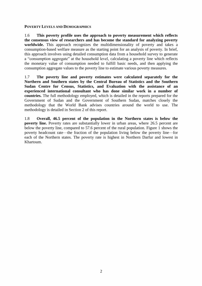
1.11 The population pyramid indicates that the Northern states have a young
population. Figure 4 shows the population pyramid. The pyramid also indicates that the sex
ratio is low for the population 20-39, i.e. the population of men is somewhat smaller than the
population of women.
Figure 4: Population Pyramid, Northern States
Source: World Bank analysis of NBHS 2009.
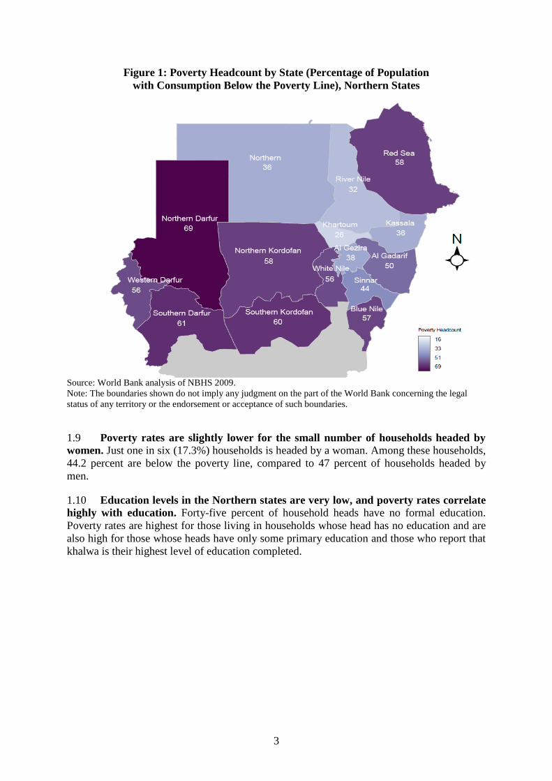
Figure 5: Percentage of Population Living in Rural Areas by State, Northern States
Source: World Bank analysis of NBHS 2009.
Note: The boundaries shown do not imply any judgment on the part of the World Bank concerning the legal
status of any territory or the endorsement or acceptance of such boundaries.
Under 5
5 to 9
10 to 14
15 to 19
20 to 24
25 to 29
30 to 34
35 to 39
40 to 44
45 to 49
50 to 54
55 to 59
60 to 64
65 to 69
70 to 74
75 to 79
80 +
10 7.5 5 2.5 0 2.5 5 7.5 10 % of North Sudan Males and Females by Age Group
Males Females

6
1.12 The majority of the population of every Northern state other than Khartoum
and the Red Sea state is rural. Overall, two-thirds (64.4 percent) of the population of the
Northern states lives in rural areas. Only 19.1 percent of the population of Khartoum state
and 45 percent of the population of Red Sea state is rural. The rural fraction for the remaining
states ranges from 67.8 percent in White Nile state to 82.7 percent in Northern state.
LIVELIHOODS AND SHOCKS
1.13 A broad measure of the main sources of livelihoods indicates that households are
engaged in a variety of activities. Figure 6 shows the breakdown of main livelihoods for
each quintile—group of 20%—of the population among three main categories: agriculture
(including crop farming and animal husbandry), wages and salaries, and other (business
enterprise, property income, remittances, pension, aid, and other.) Most of the poorest
households—those in the bottom 20%—are engaged in agriculture (crop farming and animal
husbandry). Among people in the wealthiest households—those in the top quintile—nearly
half report that their household’s main livelihood is wage and salaried employment. A
considerable number report a mix of livelihood activities that fall into the ―other‖ category.
Figure 6: Main Livelihoods by Quintiles, Northern States
Source: World Bank analysis of NBHS 2009.
Note: Figures shown are the main livelihoods of the households of individuals, by quintiles of individuals. The
poorest 20% of individuals are in the poorest quintile, the next poorest 20% are in the second quintile, etc.
20
40
60
80
100
% o
f In
div
idu
als
in Q
uin
tile
Poorest Second Third Fourth Wealthiest
Quintiles of Individuals
Agriculture Wage and Salaries Other

7
1.14 There is tremendous variation by region in the extent to which the economy is
concentrated in agriculture and livestock. Figure 7 shows the percentage for each of the
Northern states. In Northern states and the states in the northeastern corner of the country,
only a minority of people live in households whose main livelihood is agriculture or
livestock. In contrast, most people living in households in the remainder of the country report
that agriculture or livestock is their main livelihood.
Figure 7: Percentage Population Living in Households Whose Main Livelihood is
Agriculture and Livestock by State, Northern States
Source: World Bank analysis of NBHS 2009.
Note: The boundaries shown do not imply any judgment on the part of the World Bank concerning the legal status
of any territory or the endorsement or acceptance of such boundaries.
8
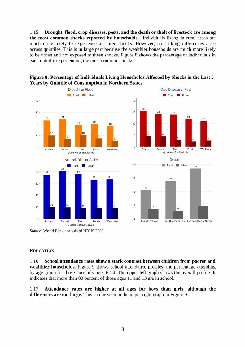
1.15 Drought, flood, crop diseases, pests, and the death or theft of livestock are among
the most common shocks reported by households. Individuals living in rural areas are
much more likely to experience all three shocks. However, no striking differences arise
across quintiles. This is in large part because the wealthier households are much more likely
to be urban and not exposed to these shocks. Figure 8 shows the percentage of individuals in
each quintile experiencing the most common shocks.
Figure 8: Percentage of Individuals Living Households Affected by Shocks in the Last 5
Years by Quintile of Consumption in Northern States
Source: World Bank analysis of NBHS 2009
EDUCATION
1.16 School attendance rates show a stark contrast between children from poorer and
wealthier households. Figure 9 shows school attendance profiles: the percentage attending
by age group for those currently ages 6-24. The upper left graph shows the overall profile. It
indicates that more than 80 percent of those ages 11 and 13 are in school.
1.17 Attendance rates are higher at all ages for boys than girls, although the
differences are not large. This can be seen in the upper right graph in Figure 9.
23
10
24
7
19
10
20
7
18
5
0
10
20
30
40
% o
f In
div
idu
als
in Q
uin
tile
Poorest Second Third Fourth Wealthiest
Quintiles of Individuals
Drought or Flood
Rural Urban
31
10
28
9
28
6
24
4
22
5
0
10
20
30
40
% o
f In
div
idu
als
in Q
uin
tile
Poorest Second Third Fourth Wealthiest
Quintiles of Individuals
Crop Disease or Pest
Rural Urban
37
10
40
10
38
9
33
9
33
9
0
10
20
30
40
% o
f In
div
idu
als
in Q
uin
tile
Poorest Second Third Fourth Wealthiest
Quintiles of Individuals
Livestock Died or Stolen
Rural Urban
21
7
28
6
37
9
0
10
20
30
40
% o
f In
div
idu
als
by S
ho
ck
Drought or Flood Crop Disease or Pest Livestock Died or Stolen
Overall
Rural Urban

9
Fig
ure
9:
Sch
ool
Att
end
an
ce b
y A
ge,
Sou
ther
n S
tate
s
So
urc
e: W
orl
d B
ank
an
aly
sis
of
NB
HS
20
09
.
100
80
60
40
20
02
04
06
08
01
00
% a
tten
din
g
24
23
22
21
20
19
18
17
16
15
14
13
12
11
10 9 8 7 6
Age
Sou
rce: N
BH
S 2
00
9
Overa
ll
Pri
mary
Secon
da
ry
Po
st
- S
eco
nd
ary
Kh
alw
a
Boys
Gir
ls
100
80
60
40
20
02
04
06
08
01
00
% a
tten
din
g
24
23
22
21
20
19
18
17
16
15
14
13
12
11
10 9 8 7 6
Age
Sou
rce: N
BH
S 2
00
9
Boys v
s G
irls
Pri
mary
Secon
da
ry
Po
st
- S
eco
nd
ary
Kh
alw
a
Urb
an
Rura
l
100
80
60
40
20
02
04
06
08
01
00
% a
tten
din
g
24
23
22
21
20
19
18
17
16
15
14
13
12
11
10 9 8 7 6
Age
Sou
rce: N
BH
S 2
00
9
Urb
an v
s R
ura
l
Pri
mary
Secon
da
ry
Po
st
- S
eco
nd
ary
Kh
alw
a
Wea
lthie
st
Poo
rest
100
80
60
40
20
02
04
06
08
01
00
% a
tten
din
g
24
23
22
21
20
19
18
17
16
15
14
13
12
11
10 9 8 7 6
Age
Sou
rce: N
BH
S 2
00
9
We
althie
st vs P
oo
rest Q
uin
tile
of
Consum
ptio
n
Pri
mary
Secon
da
ry
Po
st
- S
eco
nd
ary
Kh
alw
a
100
80
60
40
20
02
04
06
08
01
00
% a
tten
din
g
24
23
22
21
20
19
18
17
16
15
14
13
12
11
10 9 8 7 6
Age
Sou
rce: N
BH
S 2
00
9
Overa
ll
Pri
mary
Secon
da
ry
Po
st
- S
eco
nd
ary
Kh
alw
a
Boys
Gir
ls
100
80
60
40
20
02
04
06
08
01
00
% a
tten
din
g
24
23
22
21
20
19
18
17
16
15
14
13
12
11
10 9 8 7 6
Age
Sou
rce: N
BH
S 2
00
9
Boys v
s G
irls
Pri
mary
Secon
da
ry
Po
st
- S
eco
nd
ary
Kh
alw
a
Urb
an
Rura
l
100
80
60
40
20
02
04
06
08
01
00
% a
tten
din
g
24
23
22
21
20
19
18
17
16
15
14
13
12
11
10 9 8 7 6
Age
Sou
rce: N
BH
S 2
00
9
Urb
an v
s R
ura
l
Pri
mary
Secon
da
ry
Po
st
- S
eco
nd
ary
Kh
alw
a
Wea
lthie
st
Poo
rest
100
80
60
40
20
02
04
06
08
01
00
% a
tten
din
g
24
23
22
21
20
19
18
17
16
15
14
13
12
11
10 9 8 7 6
Age
Sou
rce: N
BH
S 2
00
9
We
althie
st vs P
oo
rest Q
uin
tile
of
Consum
ptio
n
Pri
mary
Secon
da
ry
Po
st
- S
eco
nd
ary
Kh
alw
a

10
1.18 At all ages, attendance rates are much higher in urban areas than in rural areas
and among children in the wealthiest quintile. The urban-rural comparison can be seen in
the lower left graph of Figure 9. The comparison of the wealthiest quintile to the poorest
quintile is shown in the lower right graph.
1.19 Attendance rates vary by state. The net primary school attendance rate measure the
fraction of children age 6-13 who are currently attending school. The net primary school
attendance rate is lowest in Kassala state (47.6%) and highest in Khartoum (85.2%).
Figure 10: Net Primary School Attendance Rates by State, Northern States
Source: World Bank analysis of NBHS 2009.
Note: Figures shown are the percentage of children ages 6-13 who are currently attending school.
The boundaries shown do not imply any judgment on the part of the World Bank concerning the legal status of any
territory or the endorsement or acceptance of such boundaries.
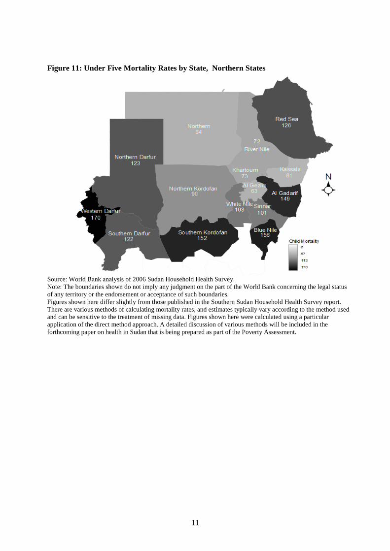
1.20 Child mortality rates are high and vary considerably by state. The child mortality
rate is the fraction of children born alive expected to die before reaching age 5, based on
recorded deaths of children during a five year period. The child mortality rate is highest in
Darfur (170) and lowest in Kassala state (61).
1.21 The child mortality figures presented here are based on the experiences from
2001-2006. It is important to recognize that child mortality is inherently measured
retrospectively. The figures presented here are based on data from the 2006 Sudan Household
Health Survey and correspond to the mortality of children born 2001-2006. It is possible that
child mortality has declined since then. Once data from the 2010 round of the Sudan
Household Health Survey is available, it will be possible to estimate child mortality rates for
the 2005-2010 period.
11
Figure 11: Under Five Mortality Rates by State, Northern States
Source: World Bank analysis of 2006 Sudan Household Health Survey.
Note: The boundaries shown do not imply any judgment on the part of the World Bank concerning the legal status
of any territory or the endorsement or acceptance of such boundaries.
Figures shown here differ slightly from those published in the Southern Sudan Household Health Survey report.
There are various methods of calculating mortality rates, and estimates typically vary according to the method used
and can be sensitive to the treatment of missing data. Figures shown here were calculated using a particular
application of the direct method approach. A detailed discussion of various methods will be included in the
forthcoming paper on health in Sudan that is being prepared as part of the Poverty Assessment.

12
FINDINGS FROM POVERTY PROFILE
1.22 The 11 figures presented in this section provide a brief overview of socioeconomic
conditions in the Northern states. The overall picture is of a society with a diverse set of
activities and substantial inequalities across space. The urban dwellers in Khartoum generally
rank among those with the top levels of indicators: low poverty rates, relativey low infant
mortality, and relative high attendance rates. A number of states have surprising mixes of
indicators. Kassala, for example, has the lowest child mortality rate among all the Northern
states but also the lowest attendance rate. Further analysis will be needed to understand the
roots of such findings.
1.23 The tables presented in the annex to this report provide additional detail for topics
presented in the 11 figures and additional areas. Topics presented in the annex tables include,
asset ownership by quintile, additional information on shocks experienced by households,
and a variety of housing information by quintile: dwelling type, sanitation facilities, energy
for cooking, and access to water.
1.24 Annex tables A3 and A4 also present results from simple regressions of consumption
and poverty on household variables. These regressions provide a useful summary of the
correlates of consumption. The results show that, holding other household characteristics
constant, larger households, and those with household heads who are less educated have
lower average levels of consumption and are thus more likely to be in poverty. Table A4
shows the change in the likelihood of being in poverty for a hypothetical household
experiencing a change in its household head. A switch from a household with no education to
some or completed primary school would make a rural household 14.3 percent less likely to
be poor.
1.25 This poverty profile represents just the beginning of the World Bank’s planned
Poverty Assessment on Sudan. Much more detailed work on education, health, employment,
and migration is forthcoming. It is hoped that this profile will provide a preliminary basis for
policy planning by authorities while the other components of the Poverty Assessment are
completed.

13
2. METHODOLOGY FOR POVERTY ANALYSIS
Note: the following is excerpted from the text of reports prepared for the Government of
Sudan and the Government of Southern Sudan by consultant Martin Cumpa. The text is
reproduced here to provide easy reference for those wishing to understand the methodology
behind the poverty figures presented in the previous section. Mr. Cumpa was hired separately
by the Government of Sudan and the Government of Southern Sudan to prepare the poverty
analysis for the Northern and Southern states. He employed the same methodology for the
Northern and Southern states analysis. His approach closely matches the general
methodology for poverty analysis recommended by the World Bank.
Despite the fact that identical methodology was employed for North and South, the separate
North and South poverty figures are not comparable. This is for two reasons: 1) the poverty
lines are different, and 2) the consumption measures have not been adjusted to reflect North-
South price differences.
First, as per the standard methodology recommended by the World Bank, the poverty lines
were constructed based on 1) calorie requirements, 2) the food consumption patterns for
typical households in the population, 3) food prices, and 4) the share of non-food items in
overall consumption. Of these inputs, (2), (3), and (4) all differ between North and South.
Consequently, the poverty lines differ markedly.
Second, as per the standard methodology recommended by the World Bank, the value of total
consumption for each household was adjusted to take into account differences in prices
across space within the North and within the South. To compare levels of consumption (and
poverty) between the North and South, it will be necessary to further adjust for price
differences between North and South.
It will be possible to directly compare poverty and consumption levels between North and
South once an overall national poverty line is constructed, the consumption aggregate is
adjusted for North-South price differences, and a unified North-South data is assembled.
2.1 Poverty refers to a pronounced deprivation in one or more dimensions of the welfare
of an individual, such as limited access to health facilities, low human capital, inadequate
housing infrastructure, malnutrition, lack of certain goods and services, inability to express
political views or profess religious beliefs, etc. Each of them deserves separate attention as
they concern different components of welfare, and indeed may help policy makers to focus
attention on the various facets of poverty. Nonetheless, often there is a high degree of
overlapping. For instance, in most contexts, a malnourished person is also poorly educated
and without access to health care.
2.2 Research on poverty over the last years has reached some consensus on using
economic measures of living standards and these are routinely employed on poverty analysis.
Moreover, monetary-based poverty indicators are the basis to monitor the first of the

14
Millennium Development Goals. This report focuses on consumption-poverty i.e. poverty
will be measured in terms of total consumption per person. Although it captures a central
component of any assessment of living standards, it does not cover all aspects of human
welfare.
2.3 Poverty analysis requires three main elements:
1. A welfare indicator, both measurable and acceptable, to rank all population
accordingly.
2. An appropriate poverty line to be compared against the chosen welfare indicator in
order to classify individuals as poor and non-poor.
3. A set of measures that combine the individual welfare indicators and the poverty line
into aggregate poverty figures.
2.4 This section explains all the steps involved in the construction of the consumption
aggregate, the derivation of the poverty line and the poverty measures. It reviews the
arguments for choosing consumption as the preferred welfare indicator, describes the
estimation of the nominal household consumption, explains how we arrive at an individual
measure of real consumption by correcting for differences in location, interview dates and
demographic composition of households, describes spatial and temporal price adjustment,
and clarifies the derivation of the poverty line.
THE CHOICE OF THE MONETARY INDICATOR
2.5 The main decision in poverty estimation is to choose between income and
consumption as the welfare indicator to determine poverty. Consumption is the preferred
measure because it is likely to be a more useful and accurate measure of living standards than
income. This preference of consumption over income is based on both theoretical and
practical issues.1
2.6 The first theoretical consideration is that both consumption and income can be
approximations to utility2, even though they are different concepts. Consumption measures
what individuals have actually acquired, while income, together with assets, measures the
potential claims of a person. Secondly, the time period over which living standards are to be
measured is important: if one is using a long term perspective as in a lifetime period, both
should be the same and the choice does not matter. In the short-run though, say a year,
consumption is likely to be more stable than income. Households are often able to smooth out
their consumption, which may reflect access to credit or savings as well as information on
future streams of income. Consumption is also less affected by seasonal patterns than income:
for example, in agricultural economies, income is more volatile and affected by growing and
harvest seasons, hence relying on that indicator might under or overestimate significantly
living standards.
1 See Deaton and Zaidi (2002), Haughton and Khandker (2009) and Hentschel and Lanjouw (1996).
2 ―Utility‖ in economics refers, loosely speaking, to the satisfaction attained from the consumption of a basket of
goods and services.

15
2.7 There are also practical arguments to take into account. First, consumption is
generally an easier concept than income for the respondents to grasp, especially if the latter is
from self-employment or family-owned businesses. For instance, workers in formal sectors of
the economy will have no problem in reporting accurately their main source of income, i.e.,
their wage or salary. But self-employed persons in informal sectors, or engaged in
agriculture, will have a harder time coming up with a precise measure of their income. Often
in these cases, household and business transactions are intertwined. Besides, as was
mentioned before, seasonal considerations are to be included to estimate an annual income
figure. Finally, we also need to consider the degree of reliability of the information.
Households are less reluctant to share information on consumption than on income. They
may be afraid than income information will be used for different purposes, say taxes, or they
may just considered income questions as too intrusive. It is also likely that household
members know more about the household consumption than the level and sources of
household income.
THE CONSTRUCTION OF THE CONSUMPTION AGGREGATE
2.8 Creating the consumption aggregate is also guided by theoretical and practical
considerations. In the case of the NBHS, the focus will be on the consumption aggregate of
the household in the last year. First, it must be as comprehensive as possible given the
available information. Omitting some components assumes that they do not contribute to
people’s welfare or that they do no affect the rankings of individuals. Second, market and
non-market transactions are to be included, which means that purchases are not the sole
component of the indicator. Third, expenditure is not consumption. For perishable goods,
mostly food, it is usual to assume that all purchases are consumed. But for other goods and
services, such as housing or durable goods, corrections have to be made. Lastly, the
consumption aggregate comprises five main components: food, non-food, durable goods,
housing and energy. The specific items included in each component and the methodology
used to assign a consumption value to each of these items is outlined below.
Food component
2.9 The food component can be constructed by simply adding up the consumption of all
food items in the household, previously normalized to a uniform reference period. The NBHS
records information on food consumption at the household level using a recall period for the
last seven days. It collects data on 150 items, which are organized in 14 categories: bread and
cereals; meat; fish and seafood; milk, cheese and eggs; oils and fats; fruits; pulses; sugar, jam
and sweets; other food items; coffee, tea and cocoa; water and drinks; tobacco; restaurants
and cafes; and food from street vendors.
2.10 A few general principles are applied in the construction of this component. First, all
possible sources of consumption are included, which means that the food component
comprises not only consumption out of purchases, or from meals eaten away from home, but
also food from previous stocks, that was produced within the household or received as a gift.
Second, only food that was actually consumed, as opposed to total food purchases or total
home-produced food, enters in the consumption aggregate. Third, non-purchased food items
need to be valued and included in the welfare measure. The survey collects information on
food purchases, thus it is possible to estimate a unit value for each food item by dividing the

16
amount paid by the quantity purchased. Ideally food items will be disaggregated enough to be
regarded as relatively homogeneous within each category, however these unit values will also
reflect differences in the quality of the good. To minimize this effect and to consider spatial
differences, median unit values were computed at several levels: urban and rural areas within
states, state, urban and rural areas, and for the entire Southern Sudan. Hence if a household
consumed a food item not purchased in the last week, the median unit value from the urban or
rural area from that state would be used to value that consumption. If no other household
consumed the same item in that area or if there were not enough observations to obtain a
reliable unit value, the median unit value from the immediate upper level was used to
estimate the value of that consumption.
2.11 A critical issue that had to be dealt with was the variety of quantity unit codes in
which households could report their purchases and consumption. The questionnaire explicitly
recognizes 18 different quantity unit codes, ranging from standard units as kilograms and
litres to less standard units as heaps, bundles, cups, rubus, bottles and sacks. The way to
address this matter was to conduct a supplementary survey and weight all these non-standard
units for the 83 most consumed items. Even when the dispersion within each non-standard
unit could be non-negligible (for instance, heaps could be small, medium or big), this allowed
the conversion of all purchases and consumption into kilograms and litres and simplified the
estimation of unit values to impute a monetary value to all food consumption that was not
purchased.
Non-food component
2.12 As in the case of food, non-food consumption is a simple and straightforward
calculation. Again, all possible sources of consumption must be included and normalized to a
common reference period. Data on an extensive range of non-food items are available, 133
items arranged in groups such as clothing and footwear, education, health, beauty and toilet
articles, recreational expenses, household goods, durable goods, housing expenditures,
transportation, communication and insurance. The survey does not gather information on
quantities consumed because most non-food items are too heterogeneous to try to calculate
unit values. This subsection covers the consumption of most non-food items while durable
goods, housing and energy will be dealt with later.
2.13 Practical difficulties arise often for two reasons: the choice of items to include and the
selection of the recall period. Regarding the first issue, the rule of thumb is that only items
that contribute to the consumption of the household are to be included. For instance, clothing,
footwear, beauty articles and recreation are included. Others such as taxes are commonly
excluded because they are not linked to higher levels of consumption, that is, households
paying more taxes are not likely to receive better public services than, say, houses which paid
lower taxes in the same community. Capital transactions like purchases of financial assets,
debt and interest payments should also be excluded. The case for lumpy or infrequent
expenditures like marriages, dowries, births and funerals is more difficult. Given their
sporadic nature, the ideal approach would be to spread these expenses over the years and thus
smooth them out, otherwise the true level of welfare of the household will probably be
overestimated. Lack of information prevents us from doing that, and so they are left out from
the estimation. Finally, remittances given to other households are also excluded. The
rationale for this is to avoid double counting because these transfers almost certainly are

17
already reflected in the consumption of the recipients. Hence including them would increase
artificially living standards.
2.14 Two non-food categories deserve special attention: education and health. In the case
of education there are three issues to consider. First, some argue that if education is an
investment, it should be treated as savings and not as consumption. Benefits from attending
school are distributed not simply during the school period but during all years after. Second,
there are life-cycle considerations as educational expenses are concentrated in a particular
time of a person’s life. Say that we compare two individuals that will pay the same for their
education but one is still studying while the other finished several years ago. The current
student might seem better-off due to higher reported spending on education but that result is
just related to age and not to true differences in welfare levels. One way out would be to
smooth these expenses over the whole life period but that option is not available for our data
since we only observe the individuals at one point in time. Third, we must consider the
coverage in the supply of public education. If all of the population can benefit from free or
heavily subsidized education and the decision of studying in private schools is driven by
quality factors, differences in expenditures can be associated with differences in welfare
levels and the case for their inclusion is stronger. Standard practice was followed and
educational expenses were included in the consumption aggregate. Excluding them would
make no distinction between two households with children in school age, but only one being
able to send them to school.
2.15 Health expenses share some of the features of education. Expenditures on preventive
health care could be considered as investments. Differences in access to publicly provided
services may distort comparisons across households. If some sectors of the population have
access to free or significantly subsidized health services, whereas others have to rely on
private services, differences in expenditures do not correspond to differences in welfare. But
there are other factors to take into account. First, health expenditures are habitually infrequent
and lumpy over the reference period. Second, health may be seen as a ―regrettable necessity‖,
i.e. the inclusion of health expenditures incurred due to the illness of a household member in
the welfare indicator implies that the welfare of that household has increased when in fact the
opposite has happened. Third, health insurance can also distort comparisons. Insured
households may register small expenditures when some member has fallen sick, while
uninsured ones bigger amounts; this is less of a concern in Sudan due to low penetration of
health insurance. It was decided to include health expenses because, as in the case of
education, their exclusion would imply making no distinction between two households, both
facing the same health problems, but only one paying for treatment.
2.16 The second difficulty regarding non-food consumption is related with the selection of
the recall period. The key aspect to consider is the relationship between recall periods and
frequency of purchases. Most non-food items are not purchased frequently enough to justify a
weekly recall period, hence generally recall periods refer to the last month, the last quarter or
the last year. The NBHS collects information with two reference periods: last 30 days and last
365 days. Those non-food items that are purchased or paid more frequently will fall into the
last month recall period (toilet and personal care items, transportation, household utilities),
whereas those less common will go into the last year reference period (clothing and footwear,
purchase and repair of household appliances, educational expenses). It was not necessary to
choose one recall period over the other because each item was asked only for one recall
period. Thus non-food consumption involved adding up all non-food expenditures, previously
normalized to a common reference period.

18
Durable goods
2.17 Ownership of durable goods could be an important component of the welfare of the
households. Given that these goods last typically for many years, the expenditure on
purchases is not the proper indicator to consider. The right measure to estimate, for
consumption purposes, is the stream of services that households derive from all durable
goods in their possession over the relevant reference period. This flow of utility is
unobservable but it can be assumed to be proportional to the value of the good. The NBHS
provides information on eight durable goods: televisions, radios, telephones, computers,
refrigerators, fans, air conditioners and mosquito nets. The survey asks about the number of
items owned by the household and their current market value, but unfortunately it does not
ask about their age. Calculating this consumption component would have involved making
assumptions about not only the depreciation rates for these eight durable goods but also the
average age of each durable good owned by the household. This may result in an extremely
imprecise estimation, thus it was decided to exclude this component from the consumption
aggregate.
Housing
2.18 Housing conditions are considered an essential part of people’s living standards.
Nonetheless, in most developing countries limited or non-existent housing rental markets
pose a difficult challenge for the estimation and inclusion of this component in the
consumption aggregate. As in the case of durable goods, the objective is to try to measure the
flow of services received by the household from occupying its dwelling. When a household
rents its dwelling, and provided rental markets function well, that value would be the actual
rent paid. If enough people rent their dwellings, that information could be used to impute
rents for those that own their dwellings. On the other hand, if the household does not rent is
dwelling, the survey asked how much would they would be willing to pay if they had to rent
it. Data on self-reported imputed rent can also be used as an alternative to data on actual
rents. Unfortunately estimating a housing component in Sudan may be particularly difficult
for two reasons. First, few households rent their dwellings, which means that rental markets
are developed at all and more likely they are concentrated in a few cities. Second, even when
the NBHS provides information on imputed rent, these data may not be that credible
considering that renting a dwelling is not common in most of the country. This will be
particularly more serious in rural areas, which account for the large majority of the
population. It was decided to exclude this component from the consumption aggregate
because its estimation may be quite imprecise. The exclusion of the imputed value of housing
is not expected to significantly change the relative ranking of the population in terms of total
consumption.
Energy
2.19 The final non-food component that justified special attention was energy
consumption, that is, expenditures on energy sources for lighting and cooking such as
electricity, gas, generator fuel, kerosene, charcoal and firewood. The NBHS collects
information about the last 30 days on purchases, consumption out of these purchases, and

19
consumption out of previous stocks, own-production, gifts and other sources. Most
households reported some energy consumption. In order to overcome this lack of
information, a regression was run to impute energy expenditures to those households that did
not report anything. Consumption on all energy sources was taken from households reporting
expenditures and correlated with the type of dwelling, the number of household members, the
per capita number of rooms in the dwelling, whether the area was urban or rural, the state and
the main source for lighting and cooking. The predicted energy consumption was imputed for
households not reporting any energy consumption.
PRICE ADJUSTMENT
2.20 Nominal consumption of the household must be adjusted for cost-of-living
differences. A temporal and a spatial price adjustment are required to adjust consumption to
real terms. In the case of the NBHS, it was decided not to adjust nominal consumption over
time because the fieldwork took place over 6 weeks, thus the inflation during that period was
considered negligible. In other words, the amount of goods and services a person could buy
in week 1 of the fieldwork with, say, 100 Sudanese Pounds was assumed to be the same as in
week 7. On the other hand, prices are expected to differ markedly across geographical
domains. It was considered that that a spatial price index by urban and rural areas would
capture properly the spatial price differences. In other words, the initial assumption is that the
purchasing power of 100 Sudanese Pounds in cities and towns is different from that in the
countryside.
2.21 A Laspeyres price index for urban and rural areas was constructed using information
from the survey and employing the following formula:
Li w0kk1
n
pik
p0k
where w0k is the national budget share of item k, pik is the median price of item k in urban or
rural areas, and p0k is the national median price of item k.
2.22 This price index compares the cost of a national bundle of goods and services using
national prices with the cost of the same bundle in urban and in rural areas. Given that the
bundle will be the same for both areas, it follows that this price index can vary only because
of differences in prices.
2.23 The NBHS provides information on budget shares for all items. In the case of food, it
is possible to estimate unit values for most food items and match them with their respective
budget shares. However, in the case of non-food, it is not possible to calculate any sort of
prices. Two assumptions were required to circumvent this problem. First, all non-food items
were bundled together, that is, they were treated as a single good. Second, the price of this
sole non-food item was the same in urban and rural areas. These two assumptions are not
expected to have significant consequences.

20
THE POVERTY LINE
2.24 The poverty line can be defined as the monetary cost to a given person, at a given
place and time, of a reference level of welfare.3 If a person does not attain that minimum
level of standard of living, she will be considered poor. Implementing this definition is,
however, not straight-forward because considerable disagreement could be encountered at
determining both the minimum level of welfare and the estimated cost of achieving that level.
In addition, setting poverty lines could be a very controversial issue because of its potential
effects on monitoring poverty and policy-making decisions.
2.25 It will be assumed that the level of welfare implied by the poverty line should enable
the individual to achieve certain capabilities, which include a healthy and active life and a full
participation in society. The poverty line will be absolute because it fixes this given welfare
level, or standard of living, over the domain of analysis. This guarantees that comparisons
across individuals will be consistent, for instance, two persons with the same welfare level
will be treated the same way regardless of the location where they live. Second, the reference
utility level has been anchored to certain attainments, in this particular case to the attainment
of the necessary calories to have a healthy and active life. Finally, the poverty line will be set
as the minimum cost of achieving that requirement.
2.26 The Cost of Basic Needs method was employed to estimate the nutrition-based
poverty line. This approach calculates the cost of obtaining a consumption bundle believed to
be adequate for basic consumption needs. If a person cannot afford the cost of the basket, this
person will be considered to be poor. First, it shall be kept in mind that the poverty status
focuses on whether the person has the means to acquire the consumption bundle and not on
whether its actual consumption met those requirements. Second, nutritional references are
used to set the utility level but nutritional status is not the welfare indicator. Otherwise, it will
suffice to calculate caloric intakes and compare them against the nutritional threshold. Third,
the consumption basket can be set normatively or to reflect prevailing consumption patterns.
The latter is undoubtedly a better alternative. Lastly, the poverty line comprises two main
components: food and non-food.
Food component
2.27 The first step in setting this component is to determine the nutritional requirements
deemed to be appropriate for being healthy and able to participate in society. Clearly, it is
rather difficult to arrive to a consensus on what could be considered as a healthy and active
life, and hence to assign caloric requirements. Besides, these requirements vary by person, by
his/her level of activity, the climate, etc.4 Common practice is to establish thresholds of
around 2,100 to 3,000 calories per person per day. The majority of the population lives in
rural areas, thus it was decided to set the daily energy intake at 2,400 calories per person per
day, which is not an uncommon threshold for the countryside.
3 Ravallion (1998) and Ravallion (1996).
4 Food and Agriculture Organization of the United Nations (2001, 2003).

21
2.28 Second, a food bundle must be chosen. In theory, infinite food bundles can provide
that amount of calories. One way out of this is to take into consideration the existing food
consumption patterns of a reference group in the country. It was decided to use the bottom
60% of the population, ranked in terms of real per capita consumption, and obtain its average
consumed food bundle. It is better to try to capture the consumption pattern of the population
located in the low end of the welfare distribution because it will probably reflect better the
preferences of the poor. Hence the reference group can be seen as a first guess of the poverty
incidence5. Third, calorific conversion factors were used to transform the food bundle into
calories. Tobacco, residual categories and meals eaten outside the household were excluded
from this calculation: the first because is not really a food item and the other two because it is
very difficult to approximate calorific intakes for them. For all of the remaining food items, it
was possible to assign a calorific factor. Fourth, median unit values were derived in order to
price the food bundle. Unit values were computed using only market transactions from the
reference group. Again, this will capture more accurately the prices faced by the poor. Fifth,
the average calorific intake of the food bundle was estimated, so the value of the food bundle
could be scaled proportionately to achieve 2,400 calories per person per day.
Non-food component
2.29 Setting this component of the poverty line is far from being a straightforward
procedure. There is considerable disagreement on what sort of items should be included in
the non-food share of the poverty line. However, it is possible to link this component with the
normative judgment involved when choosing the food component. Being healthy and able to
participate in society requires spending on shelter, clothing, health care, recreation, etc. The
advantage of using the NBHS is that the non-food allowance can also be based on prevailing
consumption patterns of a reference group and no pre-determined non-food bundle is
required.
2.30 The initial step is to choose a reference group that will represent the poor and
calculate how much they spend on non-food goods and services. This reference group will be
the population whose food consumption is similar to the food poverty line. The rationale
behind this reference group is that if an individual spends in food what was considered the
minimum for being healthy and maintaining certain activity levels, it will be assumed that
this person has also acquired the minimum non-food goods and services to support this
lifestyle.
2.31 Different ways are suggested in the literature to determine the average non-food
consumption of those with a food spending similar to the food poverty line. One option is to
rely on econometric techniques to estimate the Engel curve, that is, the relationship between
food spending and total expenditures. However, a simple non-parametric calculation as
suggested in Ravallion (1998) was followed. The procedure starts by estimating the average
5 More precisely, using the consumption pattern of the bottom 60% of the population to calculate the food
bundle implies that both the composition of consumption, i.e. the proportion of various items in total food
consumption, and the food prices faced by the poor and the bottom 60% of the population are not significantly
different.

22
non-food consumption of the population whose food expenditures lie within plus and minus
1% of the food poverty line. The same exercise is then repeated for the population lying plus
and minus 2%, 3%, and up to 10%. Second, these ten mean non-food allowances are
averaged and that will be the final non-food poverty line. Finally, the total poverty line can be
easily estimated by adding the food poverty line with the non-food poverty line.6 The
advantage of this method is that no assumptions are made on the functional form of the Engel
curve and that weights decline linearly around the food poverty line; this means that the
closer a household is to the food poverty line, the higher is its assigned weight.
2.32 The various assumptions explicitly made in this section should caution the reader
against potentially erroneous comparisons of poverty measures across countries. Poverty
estimates are sensitive to the specific methodological assumptions which are made, especially
with regard to the calorific threshold, the adjustment for household size, the economies of
scale and proportion of population chosen for selecting the food bundle. Additionally,
because food bundles are different across countries, and may therefore imply a different cost
to acquiring even the same number of calories, it is erroneous to immediately compare
poverty incidence across countries. These considerations make comparison of poverty
estimates, even with neighbouring countries, hazardous. For example, it may be cheaper to
acquire 2,400 kcal if the main staple is sorghum, in comparison to ―matooke‖ as in parts of
Uganda. Similarly, Uganda uses 3,000 kcal as the calorific threshold instead of the 2,400 kcal
applied here – clearly, estimates of poverty would increase with an increase in the calorific
threshold. The major purpose of poverty estimation using the above methodology is to rank
the various geographical and/or administrative domains, in this case states, according to the
estimated incidence of poverty and to track the trends in poverty over time. While our
analysis is suitable for the first purpose, and can be used as a basis for comparisons over time
after successive rounds are completed, it may not be suitable for comparisons across
countries.
POVERTY MEASURES
2.33 The literature on poverty measurement is extensive, but attention will focus on the
class of poverty measures proposed by Foster, Greer and Thorbecke (1984). This family of
measures can be summarized by the following equation:
q
i
i
z
yznP
1
)/1(
where is some non-negative parameter, z is the poverty line, y denotes consumption, i
represents individuals, n is the total number of individuals in the population, and q is the
number of individuals with consumption below the poverty line.
6 An equivalent way of estimating the total poverty line requires calculating the food share of the reference
group. The total poverty line will be the ratio between the food poverty line and the food share of the reference
group.

23
2.34 The headcount index (=0) gives the share of the poor in the total population, that is,
it measures the percentage of population whose consumption is below the poverty line. This is
the most widely used poverty measure mainly because it is very simple to understand and easy
to interpret. However, it has some limitations. It takes into account neither how close or far the
consumption levels of the poor are with respect to the poverty line, nor the distribution of
consumption among the poor. The poverty gap (=1) is the average consumption shortfall of
the population relative to the poverty line. Since the greater the shortfall, the higher the gap,
this measure overcomes the first limitation of the headcount. Finally, the severity of poverty
(=2) is sensitive to the distribution of consumption among the poor, a transfer from a poor
person to somebody less poor may leave unaffected the headcount or the poverty gap but will
increase this measure. The larger the poverty gap is, the higher the weight it carries.
2.35 These measures satisfy some convenient properties. First, they are able to combine
individual indicators of welfare into aggregate measures of poverty. Second, they are additive
in the sense that the aggregate poverty level is equal to the population-weighted sum of the
poverty levels of all subgroups of the population. Third, the poverty gap and the severity of
poverty satisfy the monotonicity axiom, which states that even if the number of the poor is
the same, but there is a welfare reduction in a poor household, the measure of poverty should
increase. And fourth, the severity of poverty will also comply with the transfer axiom: it is
not only the average welfare of the poor that influences the level of poverty, but also its
distribution. In particular, if there is a transfer from one poor household to a richer household,
the degree of poverty should increase.7
7 Sen (1976) formulated the monotonicity and the transfer axioms.

24
REFERENCES
Deaton, A., 1997. The Analysis of Household Surveys: A micro econometric Approach to
development policy. Baltimore and London: The World Bank, The John Hopkins University
Press.
Deaton A. and Muellbauer J., 1986. On measuring child costs: with applications to poor
countries. Journal of Political Economy 94, 720 -44.
Deaton A. and Zaidi S., 2002. Guidelines for Constructing Consumption Aggregates for
Welfare Analysis. LSMS Working Paper 135, World Bank, Washington, DC.
Food and Agriculture Organization of the United Nations , 2003. Human energy
requirements. Report of a joint FAO/WHO/UNU Expert Consultation, Rome.
Food and Agriculture Organization of the United Nations, 2003. Food – energy methods of
analysis and conversion factors. Food and Nutrition Paper 77, Rome.
Foster J., Greer E. and Thorbecke E., 1984. A class of decomposable poverty measures.
Econometrica, Vol. 52, No. 3, pp. 761-766.
Haughton, J. and Khander S., 2009. Handbook on Poverty and Inequality. The World Bank.
Hentschel J. and Lanjouw P., 1996. Constructing an indicator of consumption for the analysis
of poverty: Principles and Illustrations with Principles to Ecuador. LSMS Working Paper
124, World Bank, Washington, DC .
Howes S. and Lanjouw J.O., 1997. Poverty Comparisons and Household Survey Design.
LSMS Working Paper 129, World Bank Washington, DC.
Lanjouw P., Milanovic B., and Paternostro S., 1998. Poverty and the economic transition :
how do changes in economies of scale affect poverty rates for different households?. Policy
Research Working Paper Series 2009, The World Bank.
Ravallion M., 1996. Issues in Measuring and Modelling Poverty. Economic Journal, Royal
Economic Society, vol. 106(438), pages 1328-43, September.
Ravallion M., 1998. Poverty Lines in Theory and Practice. Papers 133, World Bank - Living
Standards Measurement.

25
ANNEX
Table A1: Poverty by Household Characteristics, Location and States
Source: World Bank analysis of NBHS 2009.
Poverty Headcount
Rate
Distribution of the
Poor
Distribution of the
Population
Household Head's Gender
Male 47.0% 83.6% 82.7%
Female 44.2% 16.4% 17.3%
Total 100.0% 100.0%
Household Head's
Education
No Education 59.4% 55.8% 43.7%
Some\Completed Primary 43.9% 22.0% 23.4%
Some\Completed Secondary 29.9% 11.8% 18.3%
Post Secondary 8.6% 1.1% 6.1%
Khalwa 50.6% 9.3% 8.5%
Total 100.0% 100.0%
Urban 26.5% 20.3% 35.6%
Rural 57.6% 79.7% 64.4%
Total 100.0% 100.0%
State
Northern 36.2% 1.9% 2.4%
River Nile 32.2% 2.8% 4.0%
Red Sea 57.7% 4.4% 3.6%
Kassala 36.3% 4.6% 5.9%
Al Gadarif 50.1% 5.2% 4.8%
Khartoum 26.0% 10.4% 18.7%
Al Gezira 37.8% 9.9% 12.2%
White Nile 55.5% 7.6% 6.4%
Sinnar 44.1% 4.3% 4.5%
Blue Nile 56.5% 3.7% 3.1%
Northern Kordofan 57.9% 11.0% 8.9%
Southern Kordofan 60.0% 7.1% 5.5%
Northern Darfur 69.4% 8.7% 5.9%
Western Darfur 55.6% 3.8% 3.2%
Southern Darfur 61.2% 14.6% 11.1%
Total 100.0% 100.0%

26
Table A2: Anatomy of Poverty in Northern States
Source: World Bank analysis of NBHS 2009.
Poverty
headcount
Standard
error
Poverty
gap
Standard
error
Squared
poverty
gap
Standard
error
Household Head's Gender
Male 0.470 0.012 0.163 0.006 0.078 0.003
Female 0.442 0.022 0.160 0.010 0.078 0.006
Household Head's
Education
No Education 0.594 0.013 0.227 0.007 0.114 0.005
Some\Completed Primary
School 0.439 0.018 0.139 0.008 0.063 0.005
Some\Completed Secondary
School 0.299 0.020 0.077 0.006 0.030 0.003
Post Secondary School 0.086 0.021 0.022 0.008 0.009 0.004
Khalwa 0.506 0.030 0.175 0.013 0.081 0.008
Urban 0.265 0.019 0.071 0.006 0.027 0.003
Rural 0.576 0.012 0.213 0.007 0.106 0.004
State
Northern 0.362 0.031 0.105 0.013 0.042 0.007
River Nile 0.322 0.033 0.088 0.015 0.035 0.008
Red Sea 0.577 0.050 0.249 0.037 0.137 0.028
Kassala 0.363 0.046 0.147 0.025 0.080 0.017
Al Gadarif 0.501 0.039 0.159 0.018 0.067 0.010
Khartoum 0.260 0.031 0.064 0.009 0.024 0.004
Al Gezira 0.378 0.037 0.101 0.013 0.041 0.007
White Nile 0.555 0.043 0.176 0.021 0.078 0.012
Sinnar 0.441 0.037 0.140 0.020 0.064 0.013
Blue Nile 0.565 0.036 0.206 0.021 0.099 0.013
Northern Kordofan 0.579 0.046 0.246 0.027 0.131 0.018
Southern Kordofan 0.600 0.038 0.207 0.017 0.094 0.009
Northern Darfur 0.694 0.030 0.274 0.018 0.142 0.012
Western Darfur 0.556 0.050 0.198 0.022 0.089 0.012
Southern Darfur 0.612 0.038 0.245 0.020 0.127 0.013
All North Sudan 0.465 0.011 0.162 0.005 0.078 0.003

27
Table A3: Consumption Regressions
Source: World Bank analysis of NBHS 2009.
Notes: These are results from regressions of log (household consumption per capita) on a set of variables at the household
level. Separate regression results are shown for urban and rural areas. Omitted dummy categories in the regression are
Northern state, no education for the household head, and male household head. *** p<0.01, ** p<0.05, * p<0.1
Dependent variable: Coefficient
Standard
error Coefficient
Standard
error
Log of household consumption per capita
Household characteristics
Log of household size -0.720*** 0.09 -0.729*** 0.06
Log of household size squared 0.044 0.03 0.038** 0.02
State
Northern (omitted)
River Nile -0.069 0.06 0.060* 0.04
Red Sea -0.223*** 0.05 -0.732*** 0.05
Kassala 0.267*** 0.06 -0.102*** 0.04
Al Gadarif 0.011 0.06 -0.182*** 0.04
Khartoum 0.093* 0.05 0.031 0.06
Al Gezira 0.037 0.07 -0.068* 0.04
White Nile -0.180*** 0.06 -0.194*** 0.04
Sinnar -0.025 0.07 -0.095*** 0.04
Blue Nile -0.012 0.06 -0.305*** 0.04
Northern Kordofan 0.046 0.07 -0.447*** 0.04
Southern Kordofan -0.101 0.06 -0.223*** 0.04
Northern Darfur -0.215*** 0.07 -0.498*** 0.04
Western Darfur 0.483*** 0.07 -0.341*** 0.04
Southern Darfur 0.026 0.06 -0.410*** 0.04
Gender of the household head
Male (omitted)
Female 0.018 0.03 -0.030 0.02
Highest level of education of household head
No Education (omitted)
Some/Completed Primary 0.208*** 0.03 0.163*** 0.02
Some/Completed Secondary 0.357*** 0.03 0.278*** 0.02
Post Secondary 0.628*** 0.04 0.586*** 0.05
Khalwa 0.059 0.04 0.163*** 0.03
Intercept 6.048*** 0.09 6.000*** 0.05
Number of observations
Adjusted R2 0.38 0.36
Urban Rural
2458 5455

28
Table A4: Changes of the Probability of Being in Poverty from Changes in Household
Head Characteristics, as Predicted by Regression Results
Source: World Bank analysis of NBHS 2009.
Note: These are predicted changes of an individual’s probability of being in poverty given hypothetical changes in the
characteristics of the household head. These predicted changes are based on the consumption regressions.
Urban Rural
Education event, change in household's head education:
change from "No Education" to "Some/Completed Primary" -31.8 -14.3
change from "No Education" to "Some/Completed Secondary" -51.6 -25.3
change from "No Education" to "Post Secondary" -78.0 -54.1
change from "No Education" to "Khalwa" -9.3 -14.4

29
Table A5: Percentage of Population Living in Rural Areas by State
State % Population Rural Standard
error
Northern 82.7 (5.8)
River Nile 72.2 (6.9)
Red Sea 45 (8.6)
Kassala 71.6 (6.9)
Al Gadarif 72.1 (7.0)
Khartoum 19.1 (5.9)
Al Gezira 80.9 (6.2)
White Nile 67.8 (7.1)
Sinnar 79.5 (6.0)
Blue Nile 74.1 (6.9)
Northern
Kordofan
80 (6.1)
Southern
Kordofan
76.5 (6.4)
Northern Darfur 77.9 (6.5)
Western Darfur 81.7 (6.0)
Southern Darfur 73.5 (6.7)
All 64.4 (2.0)
Source: World Bank analysis from NBHS 2009.

30
Table A6: Main Livelihoods of the Households of Individuals by State
Source: World Bank analysis from NBHS 2009.
Note: Standard errors are shown in parentheses.
Figures shown are the percentages of individuals by state living in households which report having each of the listed
activities as their main livelihood.
State Crop
farming
Animal
husbandry
Wages
and
salaries
Owned
business
enterprises
Property
income
Remittances Pension Aid Other Total
Northern 32.8 1.4 28.4 19.7 4.3 5.9 1.8 0.8 5.0 100
(3.8) (0.5) (3.0) (3.1) (1.1) (1.2) (0.5) (0.3) (1.8)
River Nile 22.8 2.3 50.2 18.4 0.9 2.6 2.0 0.6 0.4 100
(3.6) (1.3) (3.5) (1.9) (0.5) (0.7) (0.7) (0.3) (0.3)
Red Sea 1.7 11.4 31.7 16.5 4.1 0.2 0.4 0.1 33.7 100
(0.8) (3.7) (4.0) (2.1) (1.3) (0.1) (0.3) (0.1) (4.1)
Kassala 24.1 15.2 27.9 18.8 6.1 0.6 0.2 0.7 6.5 100
(3.7) (3.0) (4.3) (2.2) (1.3) (0.3) (0.2) (0.4) (1.5)
Al Gadarif 39.6 6.7 14.2 22.0 4.9 0.8 0.6 0.3 10.8 100
(4.1) (1.9) (2.8) (2.7) (1.1) (0.4) (0.4) (0.3) (1.6)
Khartoum 1.7 1.3 63.8 23.4 4.1 1.2 1.4 0.5 2.5 100
(0.6) (0.6) (2.6) (2.3) (1.0) (0.5) (0.5) (0.3) (0.8)
Al Gezira 27.4 1.4 37.2 16.5 5.4 1.9 0.2 0.6 9.4 100
(4.3) (0.7) (3.3) (2.5) (1.2) (0.5) (0.2) (0.3) (1.8)
White Nile 24.7 1.9 31.9 15.5 3.6 1.0 0.6 0.8 19.9 100
(3.1) (0.9) (3.5) (2.3) (1.1) (0.4) (0.4) (0.3) (3.2)
Sinnar 46.4 5.0 14.2 12.2 2.0 0.6 0.3 0.3 19.0 100
(4.5) (1.9) (3.3) (2.4) (0.7) (0.3) (0.3) (0.2) (3.0)
Blue Nile 51.4 5.8 24.7 14.4 0.7 2.7 0.1 0.1 0.0 100
(5.2) (2.6) (4.3) (2.4) (0.4) (0.7) (0.1) (0.1) (0.0)
Northern Kordofan 63.8 4.8 14.0 10.5 2.0 3.6 0.2 0.3 0.7 100
(5.3) (1.6) (3.3) (2.1) (1.1) (1.0) (0.1) (0.2) (0.4)
Southern Kordofan 65.2 2.4 15.4 10.4 3.3 0.6 1.2 0.0 1.6 100
(5.0) (0.7) (3.1) (2.0) (0.9) (0.3) (0.4) (0.0) (0.6)
Northern Darfur 70.5 3.4 14.2 6.1 0.9 0.5 0.7 0.0 3.6 100
(4.6) (1.3) (3.0) (1.6) (0.4) (0.5) (0.4) (0.0) (1.1)
Western Darfur 51.7 10.1 18.0 8.8 1.8 1.9 0.0 2.2 5.5 100
(4.9) (3.0) (3.9) (2.0) (0.7) (0.6) (0.0) (1.1) (1.1)
Southern Darfur 58.8 1.7 14.1 12.1 4.5 0.1 0.0 0.0 8.7 100
(5.4) (0.7) (2.6) (2.6) (1.3) (0.1) (0.0) (0.0) (2.5)
All 35.7 4.0 31.0 15.8 3.6 1.4 0.7 0.4 7.5 100
(1.2) (0.4) (0.9) (0.7) (0.3) (0.2) (0.1) (0.1) (0.5)
31
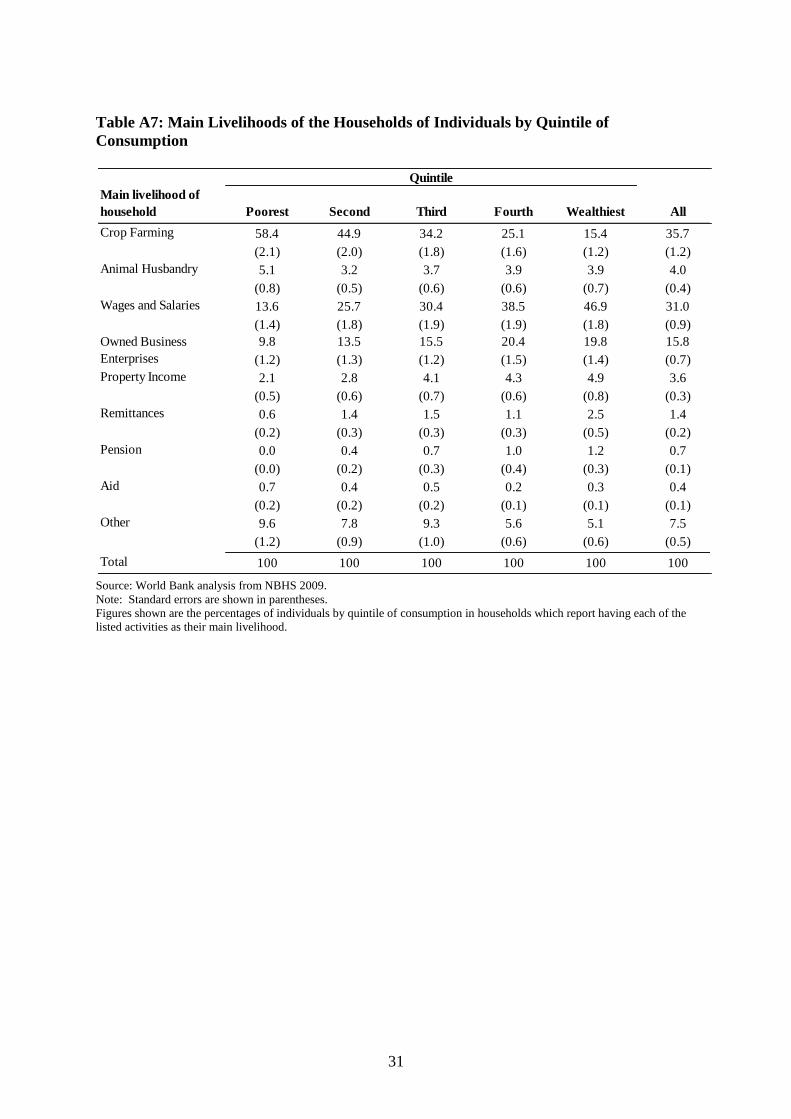
Table A7: Main Livelihoods of the Households of Individuals by Quintile of
Consumption
Source: World Bank analysis from NBHS 2009.
Note: Standard errors are shown in parentheses.
Figures shown are the percentages of individuals by quintile of consumption in households which report having each of the
listed activities as their main livelihood.
Quintile
Main livelihood of
household Poorest Second Third Fourth Wealthiest All
Crop Farming 58.4 44.9 34.2 25.1 15.4 35.7
(2.1) (2.0) (1.8) (1.6) (1.2) (1.2)
Animal Husbandry 5.1 3.2 3.7 3.9 3.9 4.0
(0.8) (0.5) (0.6) (0.6) (0.7) (0.4)
Wages and Salaries 13.6 25.7 30.4 38.5 46.9 31.0
(1.4) (1.8) (1.9) (1.9) (1.8) (0.9)
9.8 13.5 15.5 20.4 19.8 15.8
(1.2) (1.3) (1.2) (1.5) (1.4) (0.7)
Property Income 2.1 2.8 4.1 4.3 4.9 3.6
(0.5) (0.6) (0.7) (0.6) (0.8) (0.3)
Remittances 0.6 1.4 1.5 1.1 2.5 1.4
(0.2) (0.3) (0.3) (0.3) (0.5) (0.2)
Pension 0.0 0.4 0.7 1.0 1.2 0.7
(0.0) (0.2) (0.3) (0.4) (0.3) (0.1)
Aid 0.7 0.4 0.5 0.2 0.3 0.4
(0.2) (0.2) (0.2) (0.1) (0.1) (0.1)
Other 9.6 7.8 9.3 5.6 5.1 7.5
(1.2) (0.9) (1.0) (0.6) (0.6) (0.5)
Total 100 100 100 100 100 100
Owned Business
Enterprises

32
Table A9: Net Primary School Attendance Rate by State
Source: World Bank analysis of NBHS 2009.
Note: Standard errors are shown in parentheses. The net primary school attendance rate is the percentage of children age 6-
13 who are currently attending school.
State
Net primary
school
attendance Standard error
Northern 83.1 (1.8)
River Nile 83.5 (3.6)
Red Sea 67.2 (5.5)
Kassala 47.7 (6.1)
Al Gadarif 60.6 (4.7)
Khartoum 85.2 (2.7)
Al Gezira 73.1 (2.7)
White Nile 66.2 (4.2)
Sinnar 60.4 (4.6)
Blue Nile 57.1 (4.3)
Northern Kordofan 59.1 (3.8)
Southern Kordofan 60.7 (3.4)
Northern Darfur 73.0 (2.6)
Western Darfur 53.9 (4.0)
Southern Darfur 56.3 (3.8)
All 66.6 (1.1)
Table A8: Net Primary School Attendance Rate by Urban/Rural Location
Source: World Bank analysis of NBHS 2009.
Note: Standard errors are shown in parentheses. The net primary school attendance rate is the percentage of children age 6-
13 who are currently attending school.
Urban Rural All
82.3 59.3 66.6
(1.5) (1.3) (1.1)
Net primary school
attendance
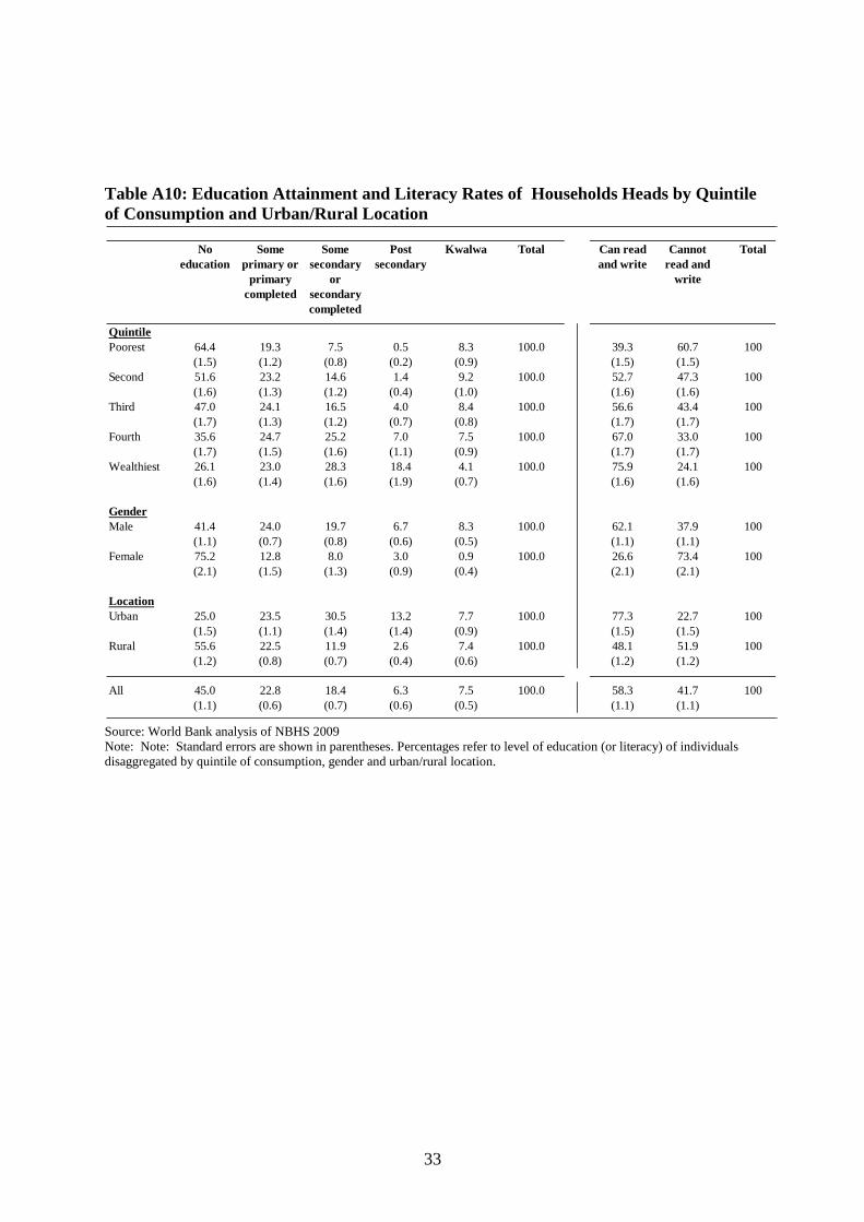
33
Table A10: Education Attainment and Literacy Rates of Households Heads by Quintile
of Consumption and Urban/Rural Location
Source: World Bank analysis of NBHS 2009
Note: Note: Standard errors are shown in parentheses. Percentages refer to level of education (or literacy) of individuals
disaggregated by quintile of consumption, gender and urban/rural location.
No
education
Some
primary or
primary
completed
Some
secondary
or
secondary
completed
Post
secondary
Kwalwa Total Can read
and write
Cannot
read and
write
Total
Quintile
Poorest 64.4 19.3 7.5 0.5 8.3 100.0 39.3 60.7 100
(1.5) (1.2) (0.8) (0.2) (0.9) (1.5) (1.5)
Second 51.6 23.2 14.6 1.4 9.2 100.0 52.7 47.3 100
(1.6) (1.3) (1.2) (0.4) (1.0) (1.6) (1.6)
Third 47.0 24.1 16.5 4.0 8.4 100.0 56.6 43.4 100
(1.7) (1.3) (1.2) (0.7) (0.8) (1.7) (1.7)
Fourth 35.6 24.7 25.2 7.0 7.5 100.0 67.0 33.0 100
(1.7) (1.5) (1.6) (1.1) (0.9) (1.7) (1.7)
Wealthiest 26.1 23.0 28.3 18.4 4.1 100.0 75.9 24.1 100
(1.6) (1.4) (1.6) (1.9) (0.7) (1.6) (1.6)
Gender
Male 41.4 24.0 19.7 6.7 8.3 100.0 62.1 37.9 100
(1.1) (0.7) (0.8) (0.6) (0.5) (1.1) (1.1)
Female 75.2 12.8 8.0 3.0 0.9 100.0 26.6 73.4 100
(2.1) (1.5) (1.3) (0.9) (0.4) (2.1) (2.1)
Location
Urban 25.0 23.5 30.5 13.2 7.7 100.0 77.3 22.7 100
(1.5) (1.1) (1.4) (1.4) (0.9) (1.5) (1.5)
Rural 55.6 22.5 11.9 2.6 7.4 100.0 48.1 51.9 100
(1.2) (0.8) (0.7) (0.4) (0.6) (1.2) (1.2)
All 45.0 22.8 18.4 6.3 7.5 100.0 58.3 41.7 100
(1.1) (0.6) (0.7) (0.6) (0.5) (1.1) (1.1)

34
Table A11: Percentage of Population Owning Assets by Quintile of Consumption
Source: World Bank analysis of NBHS 2009.
Note: Standard errors are shown in parentheses. Figures shown are the percentages of individuals in each quintile who live in
households that own each asset.
Quintile
Poorest Second Third Fourth Wealthiest All
Motor vehicle 1.3 2.7 4.6 10.4 21.9 8.2
(0.4) (0.6) (0.7) (1.2) (1.8) (0.6)
Motorcycle/motor rickshaw 1.0 1.4 2.7 3.8 4.9 2.8
(0.3) (0.4) (0.6) (0.6) (0.8) (0.3)
Bicycle 9.4 11.8 11.9 12.3 10.2 11.1
(1.2) (1.1) (1.0) (1.1) (1.1) (0.6)
Canoe/boat 0.4 0.7 0.4 0.6 0.3 0.5
(0.2) (0.2) (0.1) (0.2) (0.1) (0.1)
Animal used for transport 59.7 48.1 38.9 30.2 18.9 39.2
(2.0) (2.0) (1.7) (1.6) (1.5) (1.1)
Television/satellite dish 8.5 23.6 35.3 51.0 68.7 37.5
(1.4) (1.9) (2.2) (2.1) (2.0) (1.4)
Radio/transistor 36.1 44.8 49.9 51.7 62.1 48.9
(1.9) (1.7) (1.6) (1.7) (1.6) (1.0)
Phone 22.7 45.5 56.1 68.4 82.0 55.0
(1.9) (1.8) (1.8) (1.7) (1.3) (1.2)
Computer 0.4 0.6 1.9 5.8 13.7 4.5
(0.3) (0.2) (0.6) (1.2) (1.9) (0.6)
Refrigerator 2.2 9.9 17.6 27.7 51.4 21.8
(0.9) (1.4) (1.8) (2.1) (2.9) (1.4)
Fan 4.1 14.3 22.1 36.6 57.1 26.9
(1.2) (1.7) (2.1) (2.5) (2.7) (1.6)
Air cooler/air conditioner 0.1 1.1 3.1 6.8 23.8 7.0
(0.1) (0.4) (0.8) (1.3) (2.9) (0.9)
Pair of shoes 92.4 95.2 97.3 97.7 98.6 96.2
(1.1) (0.8) (0.5) (0.5) (0.3) (0.3)
Blanket 58.0 63.3 67.9 73.8 83.8 69.4
(2.0) (1.7) (1.7) (1.6) (1.3) (1.0)
Mosquito net 47.9 49.2 50.7 48.8 47.1 48.7
(2.2) (1.9) (1.9) (1.8) (2.0) (1.1)

35
Table A12: Percentage of Population Affected by Shocks in the Past Five Years, by
Quintile of Consumption
Source: World Bank analysis of NBHS 2009.
Note: Standard errors are shown in parentheses. Figures shown are the percentages of individuals in each quintile who live in
households that have experienced each shock.
Quintile
Poorest Second Third Fourth Wealthiest All
Drought or floods 21.3 19.6 15.9 14.2 10.0 16.2
(1.5) (1.3) (1.1) (1.1) (0.9) (0.7)
Crop diseases or pest 28.3 23.5 20.6 15.2 11.6 19.8
(1.8) (1.5) (1.4) (1.1) (1.0) (0.8)
Livestock died or stolen 33.9 32.4 28.5 22.5 18.3 27.1
(1.9) (1.6) (1.6) (1.3) (1.4) (0.8)
18.5 18.7 19.9 19.8 18.8 19.1
(1.5) (1.3) (1.3) (1.4) (1.4) (0.7)
Death of members 14.9 13.6 11.3 12.7 14.4 13.4
(1.3) (1.2) (0.9) (1.2) (1.3) (0.5)
Fire 10.2 9.5 7.6 6.4 7.4 8.2
(1.1) (1.0) (0.9) (0.7) (0.8) (0.5)
Robbery/burglary or assault 6.7 6.3 6.5 7.9 8.9 7.3
(1.0) (0.8) (0.9) (1.0) (1.0) (0.5)
Dwelling damaged/destroyed 10.2 11.9 14.9 13.5 12.1 12.5
(1.1) (1.1) (1.3) (1.3) (1.2) (0.7)
Severe water shortage 9.5 8.3 9.7 6.3 7.1 8.2
(1.4) (1.0) (1.1) (0.8) (1.0) (0.7)
Other events 2.8 3.6 2.4 2.5 1.8 2.6
(0.6) (0.7) (0.5) (0.7) (0.4) (0.2)
Illness or accidents of members

36
Table A13: Type of Dwelling by Quintile of Consumption
Source: World Bank analysis of NBHS 2009.
Note: Standard errors are shown in parentheses. Figures shown are the percentages of individuals in each quintile living in
households with each type of dwelling.
Table A14: Type of Sanitation Facility by Quintile of Consumption
Source: World Bank analysis of NBHS 2009.
Note: Standard errors are shown in parentheses. Figures shown are the percentages of individuals in each quintile living in
households with each type of toilet facility.
Quintile
Type of dwelling Poorest Second Third Fourth Wealthiest All
Dwelling from straw mats/Tent 10.8 6.6 5.0 4.7 3.0 6.0
(1.8) (0.9) (0.8) (0.8) (0.7) (0.7)
Tukul 66.4 49.2 37.4 27.6 16.6 39.5
(2.3) (1.9) (1.8) (1.5) (1.3) (1.1)
Flat/Villa/Multi-storey house 0.2 0.5 0.5 0.6 4.3 1.2
(0.1) (0.3) (0.2) (0.3) (1.5) (0.3)
House of one floor-mud 18.7 32.6 39.6 41.2 34.8 33.4
(1.8) (2.0) (2.1) (2.2) (2.7) (1.4)
House of one floor -brick/concrete 3.5 10.6 17.0 24.7 40.7 19.3
(0.9) (1.4) (1.7) (2.2) (2.8) (1.4)
House constructed of wood 0.5 0.5 0.5 1.2 0.7 0.7
(0.2) (0.2) (0.1) (0.3) (0.3) (0.1)
Total 100 100 100 100 100 100
Quintile
Main type of toilet facility Poorest Second Third Fourth Wealthiest All
Pit latrine private 42.0 51.3 57.0 61.1 55.7 53.4
(2.6) (2.1) (2.0) (2.1) (2.8) (1.5)
Shared pit latrine 3.9 6.0 7.1 6.5 7.7 6.3
(0.7) (0.8) (1.0) (0.9) (0.9) (0.5)
Private flush toilet 0.4 1.1 2.6 5.4 19.1 5.7
(0.3) (0.4) (0.7) (1.2) (2.9) (0.9)
Shared flush toilet 0.0 0.0 0.2 1.3 4.7 1.2
(0.0) (0.0) (0.1) (0.6) (1.1) (0.3)
Bucket toilet 0.0 0.1 0.4 0.4 0.2 0.2
(0.0) (0.1) (0.2) (0.2) (0.1) (0.1)
No toilet facility 53.7 41.4 32.7 25.4 12.5 33.1
(2.7) (2.0) (1.9) (1.8) (1.1) (1.4)

37
Table A15: Type of Energy for Cooking by Quintile of Consumption
Source: World Bank analysis of NBHS 2009.
Note: Standard errors are shown in parentheses. Figures shown are the percentages of individuals in each quintile living in
households using each type of energy for cooking.
Table A16: Type of Access to Drinking Water by Quintile of Consumption
Source: World Bank analysis of NBHS 2009.
Note: Standard errors are shown in parentheses. Figures shown are the percentages of individuals in each quintile living in
households reporting each of the possibilities for the household’s main access to drinking water.
Quintile
Main energy source
for cooking Poorest Second Third Fourth Wealthiest All
Firewood 82.1 61.2 45.4 32.2 19.0 48.0
(1.8) (2.1) (1.9) (1.8) (1.5) (1.3)
Charcoal 7.7 14.8 16.4 18.4 15.1 14.5
(1.1) (1.4) (1.4) (1.5) (1.6) (0.9)
Gas 8.4 22.5 36.9 48.3 64.7 36.1
(1.4) (1.7) (1.9) (2.1) (2.1) (1.2)
Electricity 0.0 0.0 0.0 0.0 0.2 0.0
(0.0) (0.0) (0.0) (0.0) (0.1) (0.0)
Paraffin 0.0 0.0 0.3 0.3 0.4 0.2
(0.0) (0.0) (0.2) (0.2) (0.2) (0.1)
Cow dung 1.5 0.9 0.6 0.4 0.2 0.7
(0.5) (0.5) (0.3) (0.2) (0.1) (0.3)
Grass 0.2 0.5 0.4 0.2 0.3 0.3
(0.1) (0.2) (0.2) (0.2) (0.1) (0.1)
Biogas 0.0 0.0 0.0 0.1 0.0 0.0
(0.0) (0.0) (0.0) (0.1) (0.0) (0.0)
No cooking 0.2 0.1 0.0 0.0 0.1 0.1
(0.1) (0.1) (0.0) (0.0) (0.1) (0.0)
Quintile
Water access Poorest Second Third Fourth Wealthiest Total
15.3 29.2 35.5 46.6 61.5 37.6
(1.8) (2.2) (2.5) (2.6) (2.9) (1.7)
Deep boreholes/Hand pumps 40.8 29.6 21.8 16.5 11.8 24.1
(2.7) (2.0) (1.6) (1.4) (1.1) (1.3)
Dam/Wells 24.2 15.0 12.8 7.3 4.7 12.8
(2.6) (1.6) (1.4) (0.9) (0.7) (1.1)
Running open water source 5.1 7.5 5.4 5.2 2.5 5.1
(0.9) (1.3) (1.0) (1.0) (0.5) (0.7)
Water vendor 14.2 18.3 23.9 24.2 19.2 19.9
(1.7) (1.7) (2.2) (2.3) (2.4) (1.5)
0.4 0.4 0.5 0.2 0.3 0.4
(0.2) (0.2) (0.5) (0.2) (0.1) (0.2)
Water filtering stations/Mechanical
boreholes
Sand filters with common network
stand
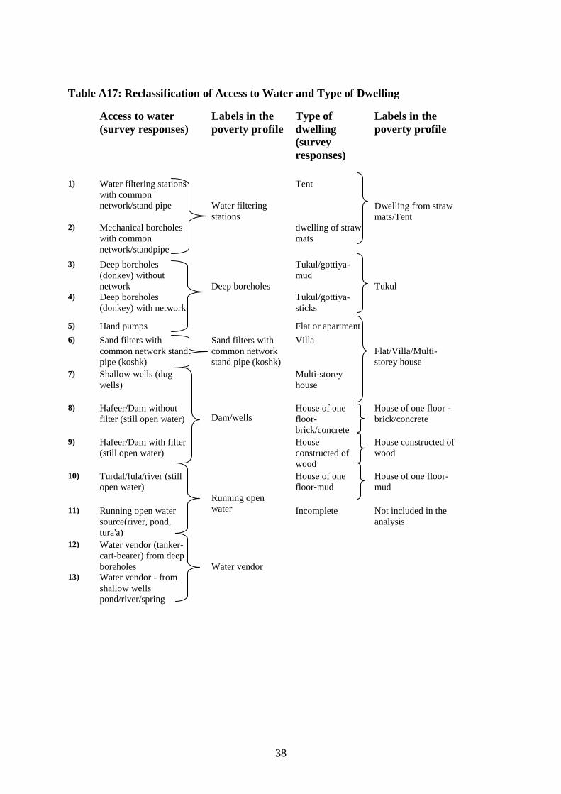
38
Table A17: Reclassification of Access to Water and Type of Dwelling
Access to water
(survey responses)
Labels in the
poverty profile
Type of
dwelling
(survey
responses)
Labels in the
poverty profile
Dwelling from straw
mats/Tent
1) Water filtering stations
with common
network/stand pipe
Water filtering
stations
Tent
2) Mechanical boreholes
with common
network/standpipe
dwelling of straw
mats
3) Deep boreholes
(donkey) without
network
Deep boreholes
Tukul/gottiya-
mud
Tukul
4) Deep boreholes
(donkey) with network
Tukul/gottiya-
sticks
5) Hand pumps Flat or apartment
6) Sand filters with
common network stand
pipe (koshk)
Sand filters with
common network
stand pipe (koshk)
Villa
Flat/Villa/Multi-
storey house
7) Shallow wells (dug
wells)
Dam/wells
Multi-storey
house
8) Hafeer/Dam without
filter (still open water)
House of one
floor-
brick/concrete
House of one floor -
brick/concrete
9) Hafeer/Dam with filter
(still open water)
House
constructed of
wood
House constructed of
wood
10) Turdal/fula/river (still
open water)
Running open
water
House of one
floor-mud
House of one floor-
mud
11) Running open water
source(river, pond,
tura'a)
Incomplete Not included in the
analysis
12) Water vendor (tanker-
cart-bearer) from deep
boreholes
Water vendor
13) Water vendor - from
shallow wells
pond/river/spring

39