A POSTERIORI ERROR ESTIMATE FOR THE CONFORMING …...A POSTERIORI ERROR ESTIMATE FOR THE H(div)...

A POSTERIORI ERROR ESTIMATE FOR THE H(div)

CONFORMING MIXED FINITE ELEMENT FOR THE COUPLED

DARCY-STOKES SYSTEM

WENBIN CHEN AND YANQIU WANG

Abstract. An H(div) conforming mixed finite element method has been pro-

posed for the coupled Darcy-Stokes flow in [30], which imposes normal con-tinuity on the velocity field strongly across the Darcy-Stokes interface. Here,we develop an a posteriori error estimator for this H(div) conforming mixedmethod, and prove its global reliability and efficiency. Due to the strong cou-

pling on the interface, special techniques need to be employed in the proof.This is the main difference between this paper and Babuska and Gatica’s work[5], in which they analyzed an a posteriori error estimator for the mixed for-

mulation using weakly coupled interface conditions.

1. Introduction

The coupled Darcy-Stokes problem is a well-known and well-studied problem,which has many important applications. We refer to the nice overview [19] andreferences therein for its physical background, modeling, and common numericalmethods. One important issue in the modeling of the coupled Darcy-Stokes flow isthe treatment of the interface condition, where the Stokes fluid meets the porousmedium. In this paper, we only consider the so called Beavers-Joseph-Saffmancondition, which was experimentally derived by Beavers and Joseph in [7], modifiedby Saffman in [40], and later mathematically verified in [27, 28, 29, 36].

Depending on whether to use the primal formulation or the mixed formulation inthe Darcy region, there are two popular ways to formulate the weak problem of thecoupled Darcy-Stokes flow. Here we concentrate on the mixed formulation, whichhas been studied in [3, 21, 22, 23, 30, 31, 32, 38, 39]. In [32], rigorous analysis of themixed formulation and its weak existence have been presented. The authors studiedtwo different mixed formulations. The first one imposes the normal continuity ofthe velocity field on the interface weakly, by using a Lagrange multiplier; whilethe second one imposes the normal continuity strongly in the functional space.Later we shall call these two mixed formulations, respectively, the weakly coupledformulation and the strongly coupled formulation.

1991 Mathematics Subject Classification. 65N15, 65N30, 76D07.Key words and phrases. mixed finite element methods, coupled Darcy-Stokes problem, a pos-

teriori estimates.Chen was supported by the Natural Science Foundation of China (11171077), the Ministry of

Education of China and the State Administration of Foreign Experts Affairs of China under the111 project grant (B08018).

Wang thanks the Key Laboratory of Mathematics for Nonlinear Sciences(EZH1411108), Fudan

University, for the support during her visit.

1

2 WENBIN CHEN AND YANQIU WANG

The weakly coupled formulation gives more freedom in choosing the discretiza-tions for the Stokes side and the Darcy side separately. The work in [21, 22, 23, 32]are based on the weakly coupled formulation. Research on the strongly coupledformulation has been focused on developing unified discretization for the coupledproblem. That is, the Stokes side and the Darcy side are discretized using the samefinite element. This approach can simplify the numerical implementation, of courseonly if the unified discretization is not significantly more complicated than com-monly used discretizations for the Darcy and the Stokes problems. One essentialdifficulty in choosing the unified discretization is that, the Stokes side velocity is inH1 while the Darcy side velocity is only in H(div). Commonly used stable finite el-ements for the Stokes equation do not work for the Darcy equation, and vice versa.Special techniques usually need to be employed. In [3], a conforming, unified finiteelement has been proposed for the strongly coupled mixed formulation. However,it is constructed only on rectangular grids, and requires special treatment of thenodal degrees of freedom along the interface. According to the authors knowledge,the element proposed in [3] is probably the only existing conforming and unifiedelement. Other researchers have resorted to less restrictive discretizations suchas the non-conforming unified approach [31] or the discontinuous Galerkin (DG)approach [30, 38, 39]. Due to its discontinuous nature, some DG discretizationsfor the coupled Darcy-Stokes problem may break the strong coupling in the dis-crete level [38, 39], as they impose the normal continuity across the interface viainterior penalties. We are interested in the H(div) conforming DG approach [30]which preserves the strong coupling even in the discrete level. The idea of theH(div) conforming DG approach is to use H(div) conforming elements, such asthe Raviart-Thomas [37] elements and the Brezzi-Douglas-Marini [9] elements, todiscretize the entire coupled problem. Such elements have normal continuity butnot tangential continuity on mesh edges/faces, and thus is not conforming for theStokes side. The solution is to use the interior penalty methods and impose thetangential continuity on the Stokes side weakly, via edge/face integrals. We pointout that the H(div) conforming interior penalty method for the Stokes equation hasbeen well-studied in [15, 16, 47]. In [30], the authors used this approach to developa discretization for the coupled Darcy-Stokes problem, which strongly satisfies thenormal continuity condition on the interface. Energy norm a priori error estimatesis also proved. Later, an L2 a priori error estimation for this approach is given [24].

The purpose of this paper is to develop an a posteriori error estimator for theH(div) conforming method proposed in [30]. A posteriori error estimations havebeen well-established for both the mixed formulation of the Darcy flow [2, 8, 11, 34],etc., and the Stokes flow [1, 6, 13, 18, 20, 26, 35, 42, 43, 45, 46], etc, among which[26, 45] covers a posteriori error estimation for H(div) conforming interior penaltymethods for Stokes equations. However, there are only a few works existing forthe coupled Darcy-Stokes problem [5, 17], where [5] concerns the weakly coupledmixed formulation while [17] uses the primal formulation on the Darcy side. To ourknowledge, there is no a posteriori error estimation for the strongly coupled mixedformulation yet for the coupled Darcy-Stokes flow.

One immediately wants to ask, how different can the a posteriori error estimationfor the strongly coupled mixed formulation be, comparing with estimations for theweakly coupled formulation or even for the pure Darcy or pure Stokes equations?

A POSTERIORI ERROR ESTIMATE FOR COUPLE DARCY-STOKES EQUATIONS 3

Here, the technical difficulty lies in the combination of a posteriori error estima-tions and the strongly imposed interface condition. For the mixed formulation ofpure Darcy problem, the easiest way of performing a posteriori error estimation isto use a Helmholtz decomposition [11], while for the interior penalty method forthe pure Stokes equation, one may want to define a continuous approximation tothe discontinuous velocity [26, 45]. When coupling these two completely differenttechniques together, the normal continuity condition across the interface needs tobe satisfied all the time. Special interpolation operators need to be constructed tofulfill this requirement, and there are many technical complexities that need to beclarified.

The paper is organized as follows. For simplicity, only two-dimensional problemsare considered. In Section 2, the model problem for the coupled Darcy-Stokes flowand its strongly coupled mixed formulation are introduced, together with severalnotations. The H(div) conforming discretization for the strongly coupled formu-lation will be presented in Section 3. Then, in Section 4, an a posteriori errorestimator is derived. The process of deriving actually also serves as the proof forthe global reliability of the estimator. The global efficiency of the estimator is ver-ified in Section 5. Finally in Appendix A, we construct an important interpolationoperator which preserves the normal continuity on the interface while satisfyingcertain properties.

2. Model problem and notation

We follow the model developed in [24, 30]. Contents of sections 2 and 3 can befound in [24, 30] and other references as will be stated. For reader’s convenience,we present some details here. The notations used in this paper are slightly differentfrom those in [24, 30], hence sections 2 and 3 also serve the purpose of introducingthe notations.

Consider the coupled Darcy-Stokes system in a polygon Ω divided into two non-overlapping subdomains ΩS and ΩD, which are occupied by the Stokes fluid andporous medium, respectively. For simplicity, assume both ΩS and ΩD are polygonal.Denote the interface between these two subdomains by ΓSD. Define ΓS = ∂ΩS\ΓSD

and ΓD = ∂ΩD\ΓSD. When the associated domain is clear from the context, use nto represent the unit outward normal vector and t the unit tangential vector suchthat (n, t) forms a right-hand coordinate system. On ΓSD, denote n to be the unitnormal vector pointing from ΩS towards ΩD, and t accordingly, as shown in Figure1.

Figure 1. Domain of the coupled Darcy-Stokes problem.

Ω

ΩD

S t

n

Γ

Γ

S

D

ΓSD


Consider the following coupled Darcy-Stokes problem, where the flow is governedby the Stokes equation in ΩS and the Darcy’s law in ΩD:

(2.1)

−∇ · T(u, p) = f in ΩS ,

K−1u+∇p = f in ΩD,

∇ · u = g in Ω.

Here u is the velocity, p is the pressure, f and g are given vector-valued and scalar-valued functions, respectively, in Ω. The stress tensor is defined by T(u, p) =2νD(u) − pI, where ν > 0 is the fluid viscosity, D(u) = 1

2 (∇u + ∇uT ) is thestrain tensor, and I is the identity matrix. Finally, K is a symmetric and uniformlypositive tensor denoting the permeability tensor divided by the fluid viscosity. Forsimplicity, assume K has smooth components and is also uniformly bounded fromabove.

To distinguish between the Darcy and the Stokes sides when necessary, we some-times denote uS = u|ΩS

, uD = u|ΩS, and pS , pD in the same fashion. The bound-

ary condition is set to be:

(2.2)uS = 0 on ΓS ,

uD · n = 0 on ΓD.

For simplicity, we assume that ΓS 6= ∅. On the interface ΓSD, we impose theconservation of mass, the balance of normal forces, and the Beavers-Joseph-Saffmancondition [7, 40]

uS · n = uD · n,(2.3)

− T(uS , pS)n · n = pD,(2.4)

− T(uS , pS)n · t = µK−1/2 uS · t,(2.5)

where µ > 0 is a variable related to the friction and shall be determined experimen-tally, K−1/2 is defined using the standard eigenvalue decomposition. We assumethat µ is smooth and uniformly bounded both above and away from zero. It is nothard to see that conditions (2.4) and (2.5) are equivalent to

(2.6) T(uS , pS)n+ pDn+ µK−1/2 (uS · t)t = 0 on ΓSD.

Due to the boundary condition (2.2), we clearly need to assume the compatibilitycondition

∫

Ωg dx = 0. In addition, the pressure is unique only up to a constant.

Thus it is convenient to assume that∫

Ω

p dx = 0.

The mixed weak formulation and the existence of the weak solution of problem(2.1) has been thoroughly discussed in [24, 32]. Below we briefly state these results.

First, we introduce several notations. For a one- or two-dimensional polygonaldomain K, denote Hs(K), where s ∈ R, to be the usual Sobolev space, with thenorm ‖ ·‖s,K . When s = 0, it coincides with the square integrable space L2(K) andwe usually suppress 0 in the subscript of the norm, that is, ‖ ·‖K = ‖ ·‖0,K . Denote(·, ·)K and < ·, · >K to be the L2 inner-product and duality form, respectively, inK. When K is one-dimensional, the convention is to use < ·, · >K for both the L2

inner-product and duality form. When K = Ω, we usually suppress the subscriptK in (·, ·)K . Finally, all these notations can be easily extended to vector and tensorspaces.


We follow the convection that a bold character denotes a vector or vector-valuedfunction. Define

H(div, K) = v ∈ (L2(K))2, ∇ · v ∈ L2(K),

with the norm

‖v‖H(div, K) = (‖v‖2K + ‖∇ · v‖2K)1/2.

Let Γ ⊂ ∂K. Define

H0,Γ(div, K) = v ∈ H(div, K), v · n = 0 on Γ,

and

H10,Γ(K) = v ∈ H1(K), v = 0 on Γ.

If Γ = ∂K, simply denote H0,∂K(div, K) = H0(div, K) and H10,∂K(K) = H1

0 (K).

We are interested in the trace of functions in H0,Γ(div, K) and H10,Γ(K) on Γ =

∂K\Γ. It is well-known that for all v ∈ H10,Γ(K), we have v|Γ ∈ H

1/200 (Γ) and for

all v ∈ H0,Γ(div, K), we have v · n|Γ ∈ (H1/200 (Γ))∗ [32] (readers may refer to [33]

for the definition and norm of H1/200 (Γ)). An important property of H

1/200 (Γ), is

that, for any function in H1/200 (Γ), it can be extended by zero on ∂K\Γ and yields

a function in H1/2(∂K).Define

V = v ∈ H0(div,Ω) |vS ∈ H1(ΩS)2 and v|ΓS

= 0.

The space V is a Hilbert space under the norm (‖v‖21,ΩS+ ‖v‖2H(div,ΩD))

1/2. Later

we will also introduce an equivalent energy norm on V . For convenience, denoteV S and V D to be the confinements of V on ΩS and ΩD respectively. It is clearthat functions in V satisfy the strong coupling condition (2.3) on the interface ΓSD.

Furthermore, vS |ΓSD∈ H

1/200 (ΓSD)2 for all v ∈ V .

Define a bilinear form a(·, ·) : V × V → R by

a(u,v) = aS(u,v) + aD(u,v) + aI(u,v),

whereaS(u,v) = 2ν(D(u), D(v))ΩS

,

aD(u,v) = (K−1u,v)ΩD,

aI(u,v) =< µK−1/2us · t,vs · t >ΓSD.

Denote Q = L20(Ω), the mean-value free subspace of L2(Ω), and define a bilinear

form b(·, ·) : V ×Q → R by

b(v, q) = −(∇ · v, q)Ω.

Now we can introduce the weak formulation of the Darcy-Stokes coupled problem:Find (u, p) ∈ V ×Q such that

(2.7)

a(u,v) + b(v, p) = (f ,v) for all v ∈ V ,

b(u, q) = −(g, q) for all q ∈ Q.

Clearly, Equation (2.7) can be written into

Λ((u, p), (v, q)) = F ((v, q)),


where

Λ((u, p), (v, q)) = a(u,v) + b(v, p) + b(u, q),(2.8)

F ((v, q)) = (f ,v)− (g, q).(2.9)

It has been shown [32] that the weak formulation (2.7) is equivalent to theboundary value problem (2.1)-(2.5). Readers may also refer to [25] for a detaileddiscussion on the interface conditions on ΓSD. To state the weak existence resultsfor problem (2.7), we first need to introduce several norms. Define an energy normon V by

‖v‖V =

(

‖∇v‖2ΩS+ ‖µ1/2K−1/4vS · t‖2ΓSD

+ ‖K−1/2v‖2ΩD+ ‖∇ · v‖2Ω

)1/2

.

It is not hard to see that

C1‖v‖V ≤

(

‖v‖21,ΩS+ ‖v‖2H(div,ΩD)

)1/2

≤ C2‖v‖V ,

where C1 and C2 depend only on the shape of domain, µ, and K. Denote ‖ · ‖Q tobe the L2 norm on Ω and

|||(v, q)||| , ‖(v, q)‖V ×Q =√

‖v‖2V

+ ‖q‖2Q.

Then, it is not hard to establish the following Ladyzhenskaya-Babuska-Brezzi con-dition [24, 32]:

a(v,v) ≥ α‖v‖2V

for all v ∈ Z,(2.10)

supv∈V

b(v, q)

‖v‖V≥ β‖q‖Q for all q ∈ Q,(2.11)

whereZ = v ∈ V | ∇ · v = 0.

These guarantee that Equation (2.7) admits a unique solution in V ×Q. Further-more, it is well-known that conditions (2.10)-(2.11) are equivalent to the followingBabuska’s form: [10]

(2.12) sup(v,q)∈V ×Q

Λ((w, ξ), (v, q))

|||(v, q)|||≥ C(α, β)|||(w, ξ)||| for all (w, ξ) ∈ V ×Q.

Here C(α, β) is a constant depending on α and β.Equation (2.7) is the strongly coupled formulation studied in [32]. An alter-

native weak formulation for problem (2.1), the weakly coupled formulation, hasalso been presented in [32]. The weakly coupled formulation is defined on the space(H1

0,ΓS(ΩS)

2×H0,ΓD(div,ΩD))×Q, and the interface condition (2.3) is then weakly

imposed by using a Lagrange multiplier. In [32], Layton, Schieweck and Yotov haveproved that when the porous medium is entirely enclosed in the fluid region, theweakly coupled formulation and the strongly coupled formulation are equivalent,and both are well-posed. However, for general domains, it can only be proved thatthe strongly coupled formulation (2.7) is well-posed, while the well-posedness of theweakly coupled formulation is unknown due to a technical difficulty of restrictingH−1/2(ΩD) on ΓSD [32]. Interested readers may refer to [32] for the details. Mixedfinite element methods introduced in [21, 22, 23, 32] are all based on the weaklycoupled formulation. The a posteriori error estimation given in [5] is also based onthe weakly coupled formulation. Different from the work in [5], here we propose


an a posteriori error estimation for the strongly coupled formulation (2.7) and itsH(div) conforming finite element discretization introduced in [24, 30].

3. Mixed finite element discretization

Recently, an H(div) conforming, unified mixed method for (2.7), in which boththe Stokes part and the Darcy part are approximated by the Raviart-Thomas (RT )elements, has been proposed [30]. Later, optimal error in L2 norm for the velocityof the H(div) conforming formulation has been proved in [24]. Of course, the RTelements are not H1 conforming on the Stokes side. The idea is to use the interiorpenalty discontinuous Galerkin H(div) approach for the Stokes equation [15, 16, 47]in the Stokes region, while using a usual mixed finite element discretization inthe Darcy region. There are three main advantages of this approach. First, theunified finite element space may simplify the numerical simulation. Second, thenormal continuity condition (2.3) on the interface is strongly imposed on the discretelevel. Third, the discretization is strongly conservative [30, 47]. For example, wheng = 0 in ΩS , then the discrete velocity is exactly divergence free, instead of weaklydivergence free. Next, we briefly present this method.

Let Th be a geometrically conformal, shape-regular mesh on Ω. We require thatTh be aligned with ΓSD. For each triangle T ∈ Th, denote by hT its diameter. Leth be the maximum of all hT . Denote T S

h and T Dh to be the meshes in ΩS and ΩD,

respectively.Denote by Eh the set of all edges in Th. For each edge e ∈ Eh, denote by he its

length. Let ESDh be the set of all edges in Th ∩ ΓSD, and let ES

h , EDh be the set of

all edges in Th ∩ (ΩS ∪ ΓS), Th ∩ (ΩD ∪ ΓD), respectively. We also denote ES0,h and

ED0,h to be the set of edges interior to ΩS and ΩD, respectively.

Let O, P be operators defined on each T ∈ T Sh or T D

h , but may not be well-defined on the entire Ω. For example, the gradient operator on the space of dis-continuous piecewise polynomials on Th. We introduce the notation for discrete L2

inner-products as following

(O(·), P(·))T Sh

=∑

T∈T Sh

(O(·), P(·))T ,

(O(·), P(·))T Dh

=∑

T∈T Dh

(O(·), P(·))T .

Similarly, define < ·, · >ESh, < ·, · >ES

0,h, < ·, · >ED

h, < ·, · >ED

0,h, and < ·, · >ESD

h

in the same fashion. With the aid of these notations, we can also denote mesh-dependent ”broken” L2 norms in a straight-forward manner. For example, ‖·‖T S

h,

(·, ·)1/2

T Sh

and ‖ · ‖ESDh

,< ·, · >1/2

ESDh

. We especially remark that the ”broken” norm

may even contain hT or he in it. For example,

‖hTv‖T Sh

= (hTv, hTv)1/2

T Sh

=

(

∑

T∈T Sh

h2T ‖v‖

2T

)1/2

,

‖h−1/2e v‖ESD

h=< h−1/2

e v, h−1/2e v >

1/2

ESDh

=

(

∑

e∈ESDh

h−1e ‖v‖2e

)1/2

.

Such notations shall greatly clean up the style of this paper.


Let V h ⊂ H0(div,Ω) and Qh ⊂ Q be a pair of the Raviart-Thomas [37] finiteelement spaces, except for the lowest-order one, defined on Th. That is, V h is theRTk space, with k ≥ 1, and Qh is the discontinuous Pk space. Notice here weexclude the RT0 element, since otherwise V h∩V will be empty. Readers may referto [10, 14] for more details and properties of the RT elements.

For convenience, denote V h,S and V h,D to be the confinement of V h in ΩS

and ΩD, respectively. Similarly, for any v ∈ V h, it can be split into vh,S ∈ V h,S

and vh,D ∈ V h,D. Denote Ph the space of H1 conforming Lagrange finite elementspace on Th consisting of piecewise polynomials with degree less than or equal tok, and let Ph,S , Ph,D be the confinements of Ph on ΩS and ΩD, respectively. Bythe definition, we have

(Ph,S)2 ∩ V S ⊂ V h,S .

Finally, we point out that all functions in V h satisfy the strong coupling condition(2.3) on the interface ΓSD.

Define a discrete bilinear form

aS,h(u,v) = 2ν

(

(D(u), D(v))T Sh− < D(u)n, [v] >ES

h− < [u], D(v)n >ES

h

+ <σ

he[u], [v] >ES

h

)

,

where · and [·] denote the average and the jump on edges, respectively, and σ > 0is a parameter of O(1). On the boundary edge e ⊂ ΓS , · and [·] are just the one-sided values. On each edge, the direction n is taken to be the same as the directionin [·], that is, if [v]|e , v|T1

−v|T2where T1 and T2 share the edge e, then n points

from T1 to T2. The notations in the definition of bilinear form aS,h are standard inthe discontinuous Galerkin literature and readers may refer to [15, 16, 30, 47] formore details.

Now, define

ah(u,v) = aS,h(u,v) + aD(u,v) + aI(u,v).

We have the discrete problem [24, 30]: Find (uh, ph) ∈ Vh ×Qh such that

(3.1)

ah(uh,v) + b(v, ph) = (f ,v) for all v ∈ V h,

b(uh, q) = −(g, q) for all q ∈ Qh.

Since V h,S is not in H10,ΓS

(ΩS)2, the discrete space V h is not a subspace of V .

Therefore it does not inherit the norm of V . Here we shall define a discrete normon V h by

‖v‖V h=

(

‖∇v‖2T Sh

+ ‖h−1/2e [v]‖2

ESh

+ ‖µ1/2K−1/4vS · t‖2ESDh

+ ‖K−1/2v‖2ΩD+ ‖∇ · v‖2Ω

)1/2

.

Although the norm ‖ · ‖V is not well-defined on V h, we point out that the discretenorm ‖ · ‖V h

is well-defined on V . Indeed, it is clear that ‖v‖V h= ‖v‖V for all

v ∈ V , since the jump term ‖h−1/2e [v]‖ES

hvanishes. Later we shall use this property

and build certain discrete functions in V . Then for these functions, one can easilyshift from the discrete ‖ · ‖V h

norm to the continuous ‖ · ‖V norm.


The space Qh is a subspace of Q and inherits its norm, which is just the L2

norm. Define the norm in (V + V h)×Q by

|||(v, q)|||h =

(

‖v‖2V h

+ ‖q‖2Q

)1/2

.

Again, we have

|||(v, q)|||h = |||(v, q)||| for all v ∈ V and q ∈ Q.

Well-posedness and a priori error estimates for (3.1) have been given in [24, 30]:

Theorem 3.1. Equation (3.1) has a unique solution (uh, ph) for σ large enough,but not depending on h. Assume the solution (u, p) of (2.7) is in Hs(Ω)2 ×Hs(Ω)with 3/2 < s ≤ k + 1,then

|||(u− uh, p− ph)|||h ≤ Chs−1(|u|s,Ω + |p|s,Ω),

where C is a positive constant independent of the mesh size.

4. Residual based a posteriori estimation

The goal of this section is to derive an a posteriori error estimator for the problem(3.1). For simplicity of notation, we shall use “.” to denote “less than or equalto up to a constant independent of the mesh size, variables, or other parametersappearing in the inequality”. In this section, we will also frequently use the followingwell-known inequality: for any function ξ ∈ H1(T ) where T is a triangle with anedge e, the following estimate holds:

(4.1) he‖ξ‖2e . ‖ξ‖2T + h2

T ‖∇ξ‖2T .

To derive an a posteriori error estimator, we first denote

εu = u− uh, εp = p− ph,

where (u, p) is the solution to (2.7) and (uh, ph) is the solution to (3.1). The ideaof deriving a reliable a posteriori error estimator is to find an upper bound for|||(εu, εp)|||h.

As pointed out in the previous section, the norms ||| · |||h and ||| · ||| are identical onV ×Q. Thus we introduce a new discrete function uh ∈ V , which is defined fromthe discrete solution uh and satisfy

(4.2) ‖uh − uh‖V h. ‖h−1/2

e [uh]‖ESh.

The definition of uh and the proof of Equation (4.2) will be given in Appendix A.Note that uh is not necessarily in V h. The term ‖uh − uh‖V h

is usually called thenonconformity estimator in the a posteriori error estimation literature.

Denote

εu = u− uh ⊂ V ,

then

|||(εu, εp)|||h ≤ ‖uh − uh‖V h+ |||(εu, εp)|||h = ‖uh − uh‖V h

+ |||(εu, εp)|||.

Since ‖uh−uh‖V his bounded in Equation (4.2), we only need to estimate |||(εu, εp)|||.

By the Babuska’s condition (2.12),

|||(εu, εp)||| . sup(v,q)∈V ×Q

Λ((εu, εp), (v, q))

|||(v, q)|||.


Note that

Λ((εu, εp), (v, q)) =

(

a(εu,v) + b(v, εp)

)

+ b(εu, q)

=

(

(f ,v)− a(uh,v)− b(v, ph)

)

+

(

− (g, q) + (∇ · uh, q)

)

= Res1(v) +Res2(q).

Here

(4.3)

Res2(q) ≤ ‖g −∇ · uh‖‖q‖ ≤

(

‖g −∇ · uh‖+ ‖uh − uh‖V h

)

‖q‖

.

(

‖g −∇ · uh‖+ ‖h−1/2e [uh]‖ES

h

)

‖q‖.

Next, we concentrate on estimating Res1(v). Let vh ∈ V h be any function, by(3.1), we have

Res1,h(vh) , (f ,vh)− ah(uh,vh)− b(vh, ph) = 0.

Thus

Res1(v) = Res1(v)−Res1,h(vh)

= (f ,v − vh)−

(

a(uh,v)− ah(uh,vh)

)

− b(v − vh, ph)

= (f ,v − vh)ΩD−

(

aD(uh,v)− aD(uh,vh)

)

+ (∇ · (v − vh), ph)ΩD

+ (f ,v − vh)ΩS−

(

aS(uh,v)− aS,h(uh,vh)

)

+ (∇ · (v − vh), ph)ΩS

−

(

aI(uh,v)− aI(uh,vh)

)

= RD +RS +RI ,

Next, we shall derive upper bounds for RD, RS and RI one by one. Clearly, thechoice of vh is essential to the estimation. We would like vh to satisfy the followingconditions:

(1) vh is in V h ∩ V ;(2) vh is a good approximation of v;(3) vh should lead to a straight-forward a posteriori error estimation, which

allows us to follow well-known techniques from the a posteriori error esti-mations of pure Darcy and pure Stokes problems.

To satisfy the third condition, we must first investigate a posteriori error estimatorsfor the pure Darcy and the pure Stokes equations. For the Stokes equations, wefollow the proof in [26] where vh is chosen to be the Clement interpolation of v.For the Darcy equation, we follow the proof in [11] where vh needs to be definedusing a Helmholtz decomposition. Now the difficulty is, how to couple these twodifferent type of definitions while ensuring that vh ∈ V h ∩ V ? Note that vh mustsatisfy the strong coupling condition (2.3) across the interface ΓSD.


4.1. Defining vh. Given v ∈ V , we define the Stokes side approximation vh,S andthe Darcy side approximation vh,D separately. Then vh will be the combination ofvh,S and vh,D as long as they satisfy

(4.4) vh,S · n = vh,D · n on ΓSD.

On the Stokes side, the approximation can be done directly by a Clement typeinterpolation onto (Ph,S)

2∩V S ⊂ V h,S . Here we pick the Scott-Zhang interpolation[41], since it also preserves the non-homogeneous boundary condition. The idea ofthe Scott-Zhang interpolation is to first assign, for each Lagrange interpolationpoint used as degrees of freedom for Ph,S , an associated integration region (seeFigure 2). Then, define the interpolated value at each Lagrange point by testingthe function with the dual basis in the associated integration region. For Lagrangepoints interior to a triangle T ∈ T S

h , the associate integration region is the triangleT . For Lagrange points lying on edges, the associate integration region is chosento be an edge. Note for points where several edges meet, the choice may not beunique. In order to preserve the boundary condition, the associated integrationregion for Lagrange points lying on ∂ΩS need to be chosen as a boundary edgeon ∂ΩS . We especially note that, at the end points ΓS ∩ ΓSD, the associatedintegration region needs to be chosen on ΓS , in order to ensure the interpolatedvalue at these points are equal to zero (see Figure 2). Denote Ih to be the Scott-Zhang interpolation mentioned above that maps H1(ΩS) to Ph,S , preserving thehomogeneous boundary condition on ΓS . On ΓSD, Ih maps the value at the endpoints of ΓSD into zero, while produces the interpolated value on ΓSD using only thefunction value on ΓSD. Indeed, Ih|ΓSD

can be viewed as a well-defined interpolation

fromH1/200 (ΓSD) to Ph|ΓSD

, by simply setting the interpolation at end-points of ΓSD

to be zero. Notice that H1/200 (ΓSD) can be extended by zero on either ΓS or ΓD, we

are able to easily make transition from ΩS to ΩD. That is, for ξ ∈ H10,ΓD

(ΩD) and

consequently ξ|ΓSD∈ H

1/200 (ΓSD), the interpolation Ih|ΓSD

ξ is also well-defined onΓSD. Furthermore, similar to the proof in [41], one can show that for any e ∈ ESD

h ,

(4.5) he‖(I − Ih|ΓSD)ξ‖2e .

∑

T∈SD(e)

h2T ‖∇ξ‖2T ,

where SD(e) is the set of triangles in T Dh that have a non-empty intersection with

e. In the rest of the paper, when there is no ambiguity, we will just denote Ih|ΓSD

by Ih.Clearly Ih , (Ih)

2 will map V S into (Ph,S)2 ∩V S ⊂ V h,S . It is also known [41]

that Ih is a projection. In other words, IhϕS = ϕS for all ϕS in (Ph,S)2 ∩ V S .

Define vh,S = IhvS . Since Ih is a linear operator, we have vh,S · n = (IhvS) · n =Ih(vS · n) on ΓSD.

On the Darcy side, the interpolation will be defined using a Helmholtz decom-position. That is, we first split

vD = w + curl η,

where

curl η =

(

− ∂η∂x2

∂η∂x1

)

,


Figure 2. Associated integration region for different type of La-grange points. Each Lagrange point is denoted by a black dot, andthe associated integration region is denoted by either a (shaded)triangle or a (bold) edge. For Lagrange points on ΓS , ΓSD, or theintersection of ΓS and ΓSD, there are special rules for choosing theassociated integration region.

ΩS

ΩS ΩS

ΩS ΩS ΩS

Lagrange points in

Lagrange points on ΓSΓS

Lagrange points on ΓSD

ΓSD ΓSD

ΓS

and w satisfies

∇ ·w = ∇ · vD,(4.6)

w|ΓD= 0, w|ΓSD

= vS |ΓSD.(4.7)

Here, condition (4.7) is imposed to ensure w ·n|ΓD= 0 and w ·n|ΓSD

= vS ·n. Thenw ·n|∂ΩD

= vD ·n|∂ΩDand consequently the compatibility condition

∫

ΩD∇·w dx =

∫

ΩD∇ · vD dx =

∫

∂ΩDvD · n ds =

∫

∂ΩDw · n ds is satisfied.

Of course one needs to make sure such a decomposition is well-defined and w, η

have certain regularity results. Indeed, since vS |ΓSD∈ H

1/200 (ΓSD)2, according to

[4], there exists such a w ∈ H1(ΩD)2 satisfying (4.6) and (4.7). Furthermore, wehave

(4.8) ‖w‖1,ΩD. ‖v‖V .

Now (vD −w)|ΩD∈ H0(div,ΩD) is divergence-free. Thus there exists a potential

function η ∈ H10 (ΩD) such that curl η = vD −w, and

(4.9) ‖η‖1,ΩD. ‖curl η‖0,ΩD

= ‖vD −w‖0,ΩD. ‖v‖V .

Now we can start to define vh,D. First, we need an interpolation operator fromH1(ΩD)2 to V h,D, which must map w · n to Ih(w · n) on ΓSD . Recall that ausual nodal value interpolation Πh : H1(ΩD)2 → V h,D associated with the degreesof freedom of the RTk elements [10] will map w · n to Ph(w · n) on ΓSD, wherePh is the L2 projection onto (V h,D · n)|ΓSD

= Ph|ΓSD. Hence, we define a new

interpolation Πh : H1(ΩD)2 → V h,D such that it is the same as Πh on all otherdegrees of freedom except for those associated with w · n|ΓSD

. On these degrees of

freedom, define Πh by

(4.10)

∫

e

(Πhw · n)sr ds =

∫

e

Ih(w · n)sr ds for all e ∈ ESDh and 0 ≤ r ≤ k.


Of course, on other degrees of freedom, Πh inherits the properties of Πh, especiallythe following ones

(4.11)

∫

e

(w − Πhw) · n qh ds = 0 for all e ∈ EDh and qh ∈ Qh,D,

∫

T

(w − Πhw) · ∇qh dx = 0 for all T ∈ T Dh and qh ∈ Qh,D.

Combine Proposition III.3.6 in [10] and approximation property of the Scott-Zhanginterpolation in [41], then use the scaling argument, Inequality (4.5), and the prop-erty of the L2 projection, we have for all T ∈ T D

h ,

(4.12)

‖w − Πhw‖0,T . ‖w −Πhw‖0,T + ‖Πhw −Πhw‖0,T

. hT ‖∇w‖T + h1/2T ‖(Ih − Ph)(w · n)‖T∩ΓSD

.

(

∑

T∈SD(T )

h2T ‖∇w‖2T

)1/2

where SD(T ) is the set of all triangles in T Dh that has a non-empty intersection

with T ∩ ΓSD.Different from Πh, which satisfies ∇ · (Πhw) = Qh(∇ ·w) (see [10]), where Qh

is the L2 projection onto Qh,D, Πh does not satisfy the same relation. Instead, for

all qh ∈ Qh,D, by the definition of Πh and its properties (4.10)-(4.11), we have

(4.13)

(∇ · (w − Πhw), qh)ΩD

=∑

T∈T Dh

(

< (w − Πhw) · n, qh >∂T −(w − Πhw,∇qh)T

)

=− < (w − Πhw) · n, qh >ESDh

=− < (I − Ih)vS · n, qh >ESDh

.

Finally, define

vh,D = Πhw + curl ηh,

where ηh is the Clement interpolation of η into the continuous piecewise Pk+1 poly-nomials on T D

h that preserves the homogeneous boundary condition on ∂ΩD. Ofcourse one can also chose ηh to be the Scott-Zhang interpolation. By the prop-erties of the Raviart-Thomas elements [10], it is easy to see that vh,D ∈ V h,D.Furthermore, vh,S and vh,D satisfy the interface coupling condition (4.4) and hencevh ∈ V h ∩ V . By the approximation properties of the Scott-Zhang interpolationIh and the Clement interpolation, we have

(4.14)

∑

T∈T Sh

(

‖vS − vh,S‖2T + h2

T |vS − vh,S |21,T

)

.∑

T∈T Sh

h2T |v|

21,T ,

∑

T∈T Dh

(

‖η − ηh‖2T + h2

T |η − ηh|21,T

)

.∑

T∈T Dh

h2T |η|

21,T .

Now we are ready to derive upper bounds, or equivalently the a posteriori errorestimators, for RD, RS and RI .


4.2. Deriving the Darcy estimator. By the definition of aD(·, ·), Equation(4.13), and the Schwarz inequality,

RD = (f ,v − vh)ΩD−

(

aD(uh,v)− aD(uh,vh)

)

+ (∇ · (v − vh), ph)ΩD

= (f ,v − vh)ΩD− (K−1(uh − uh),v)ΩD

− (K−1uh,v − vh)ΩD

+ (∇ · (v − vh), ph)ΩD

= (f −K−1uh,v − vh)ΩD− (K−1(uh − uh),v)ΩD

− < (I − Ih)vS · n, ph,D >ESDh

. (f −K−1uh,v − vh)ΩD+ ‖uh − uh‖‖v‖ΩD


.

Next, notice that

(f−K−1uh,v−vh)ΩD= (f−K−1uh,w−Πhw)ΩD

+(f−K−1uh, curl (η−ηh))ΩD,

where by (4.11), (4.12) and (4.8),

(f −K−1uh,w − Πhw)ΩD. inf

ph∈Qh,D

‖hT (f −K−1uh −∇ph)‖T Dh|w|1,ΩD

. infph∈Qh,D

‖hT (f −K−1uh −∇ph)‖T Dh‖v‖V ,

and by (4.1), (4.9), integration by parts, the boundary condition of η, and (4.14)

(f −K−1uh, curl (η − ηh))

.

(

‖hT curl (f −K−1uh)‖T Dh

+ ‖h1/2e [f −K−1uh] · t‖ED

0,h

)

|η|1,ΩD

.

(

‖hT curl (f −K−1uh)‖T Dh

+ ‖h1/2e [f −K−1uh] · t‖ED

0,h

)

‖v‖V .

Here curl is defined for any vector-valued function ξ = (ξ1, ξ2)t by

curl ξ = −∂ξ1∂x2

+∂ξ2∂x1

.

Combining the above and using (4.2), we have

RD .

(

infph∈Qh,D

‖hT (f −K−1uh −∇ph)‖T Dh

+ ‖hT curl (f −K−1uh)‖T Dh

+ ‖h1/2e [f −K−1uh] · t‖ED

0,h+ ‖h−1/2

e [uh]‖ESh

)

‖v‖V


.


4.3. Deriving the Stokes estimator. Note that [vh] = 0 on all e ∈ ESh . By using

the definition of aS(·, ·), ah,S(·, ·), and T, we have

RS = (f ,v − vh)ΩS−

(

aS(uh,v)− aS,h(uh,vh)

)

+ (∇ · (v − vh), ph)ΩS

= (f ,v − vh)ΩS+ (2νD(uh − uh), D(v))T S

h

−

(

(2νD(uh), D(v))T Sh− aS,h(uh,vh)− (phI,∇(v − vh))T S

h

)

= (f ,v − vh)ΩS+ (2νD(uh − uh), D(v))T S

h

− (T(uh, ph), D(v − vh))T Sh− 2ν < [uh], D(vh)n >ES

h

. (f ,v − vh)ΩS− (T(uh, ph),∇(v − vh))T S

h

+ ‖uh − uh‖V h‖v‖V − 2ν < [uh], D(vh)n >ES

h.

In the above we have used the algebraic relation that for any symmetric tensor τand domain K, (τ,∇(v − vh))K = (τ,D(v − vh))K .

Using integration by parts and (4.1), (4.14),

(f ,v − vh)ΩS− (T(uh, ph),∇(v − vh))T S

h

=(f +∇ · T(uh, ph),v − vh)T Sh−∑

T∈T Sh

< T(uh, ph)n,v − vh >∂T

.

(

‖hT (f +∇ · T(uh, ph))‖T Sh+ ‖h1/2

e [T(uh, ph)]n‖ES0,h

)

‖v‖V

− < T(uh, ph)n, (I − Ih)vS >ESDh

.

Combine all the above and using (4.2), we have

RS .

(

‖hT (f +∇ · T(uh, ph))‖T Sh+ ‖h1/2


+ ‖h−1/2e [uh]‖ES

h

)

‖v‖V − < T(uh,S , ph,S)n, (I − Ih)vS >ESDh

.

4.4. Deriving the interface estimator. By the definition of aI(·, ·) and usingthe Schwarz inequality, inequalities (4.1), (4.2), we have

RI = −aI(uh,v) + aI(uh,vh)

= − < µK−1/2(uh,S − uh,S) · t,vS · t >ESDh

− < µK−1/2uh,S · t, (vS − vh,S) · t >ESDh

≤ ‖uh − uh‖V h‖v‖V h

− < µK−1/2uh,S · t, (I − Ih)vS · t >ESDh

. ‖h−1/2e [uh]‖ES

h‖v‖V − < µK−1/2uh,S · t, (I − Ih)vS · t >ESD

h.


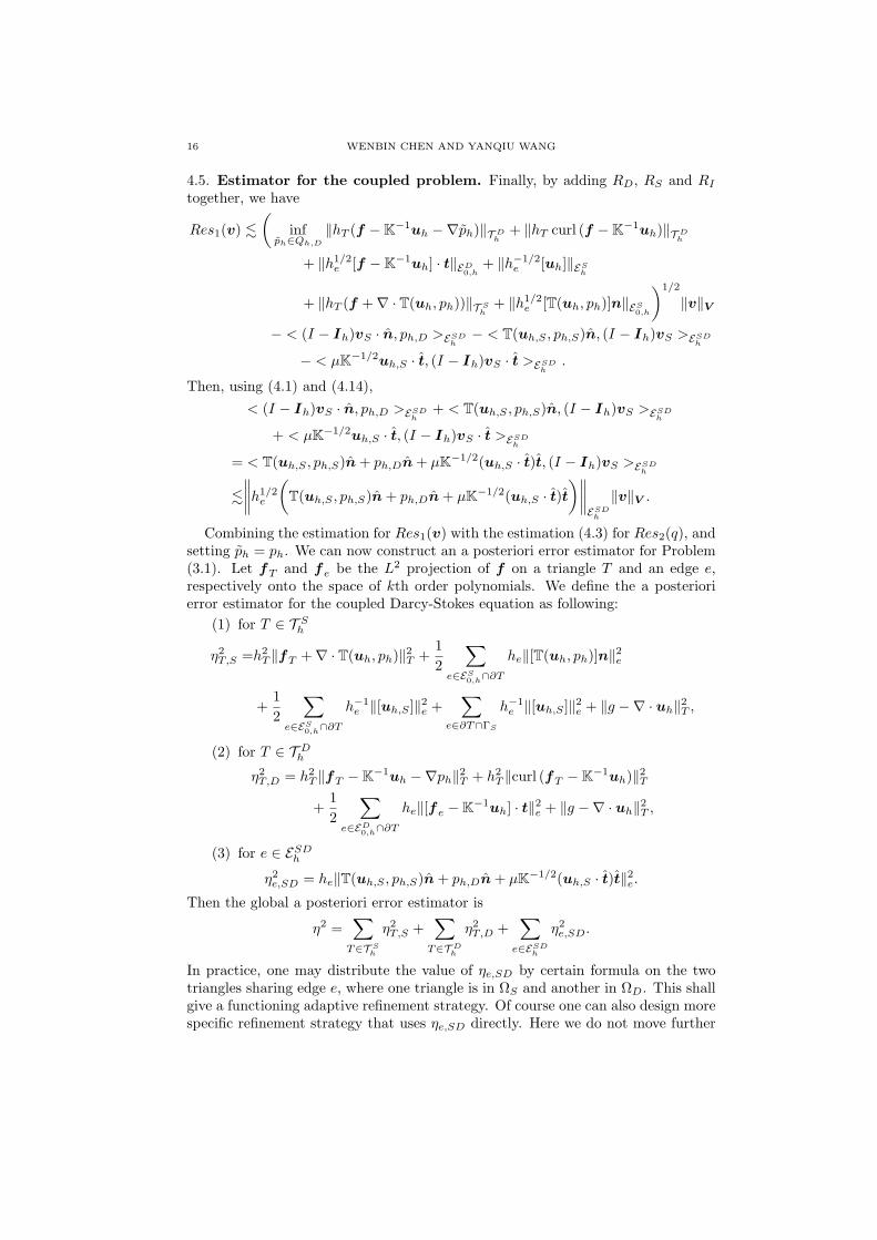
4.5. Estimator for the coupled problem. Finally, by adding RD, RS and RI

together, we have

Res1(v) .

(

infph∈Qh,D

‖hT (f −K−1uh −∇ph)‖T Dh

+ ‖hT curl (f −K−1uh)‖T Dh

+ ‖h1/2e [f −K−1uh] · t‖ED

0,h+ ‖h−1/2

e [uh]‖ESh

+ ‖hT (f +∇ · T(uh, ph))‖T Sh+ ‖h1/2


)1/2

‖v‖V


− < T(uh,S , ph,S)n, (I − Ih)vS >ESDh

− < µK−1/2uh,S · t, (I − Ih)vS · t >ESDh

.

Then, using (4.1) and (4.14),

< (I − Ih)vS · n, ph,D >ESDh

+ < T(uh,S , ph,S)n, (I − Ih)vS >ESDh

+ < µK−1/2uh,S · t, (I − Ih)vS · t >ESDh

= < T(uh,S , ph,S)n+ ph,Dn+ µK−1/2(uh,S · t)t, (I − Ih)vS >ESDh

.

∥

∥

∥

∥

h1/2e

(

T(uh,S , ph,S)n+ ph,Dn+ µK−1/2(uh,S · t)t

)∥

∥

∥

∥

ESDh

‖v‖V .

Combining the estimation for Res1(v) with the estimation (4.3) for Res2(q), andsetting ph = ph. We can now construct an a posteriori error estimator for Problem(3.1). Let fT and fe be the L2 projection of f on a triangle T and an edge e,respectively onto the space of kth order polynomials. We define the a posteriorierror estimator for the coupled Darcy-Stokes equation as following:

(1) for T ∈ T Sh

η2T,S =h2T ‖fT +∇ · T(uh, ph)‖

2T +

1

2

∑

e∈ES0,h

∩∂T

he‖[T(uh, ph)]n‖2e

+1

2

∑

e∈ES0,h

∩∂T

h−1e ‖[uh,S ]‖

2e +

∑

e∈∂T∩ΓS

h−1e ‖[uh,S ]‖

2e + ‖g −∇ · uh‖

2T ,

(2) for T ∈ T Dh

η2T,D = h2T ‖fT −K−1uh −∇ph‖

2T + h2

T ‖curl (fT −K−1uh)‖2T

+1

2

∑

e∈ED0,h

∩∂T

he‖[fe −K−1uh] · t‖2e + ‖g −∇ · uh‖

2T ,

(3) for e ∈ ESDh

η2e,SD = he‖T(uh,S , ph,S)n+ ph,Dn+ µK−1/2(uh,S · t)t‖2e.

Then the global a posteriori error estimator is

η2 =∑

T∈T Sh

η2T,S +∑

T∈T Dh

η2T,D +∑

e∈ESDh

η2e,SD.

In practice, one may distribute the value of ηe,SD by certain formula on the twotriangles sharing edge e, where one triangle is in ΩS and another in ΩD. This shallgive a functioning adaptive refinement strategy. Of course one can also design morespecific refinement strategy that uses ηe,SD directly. Here we do not move further


into the adaptive refinement strategies, since we are only interested in the globalupper and lower bounds for η.

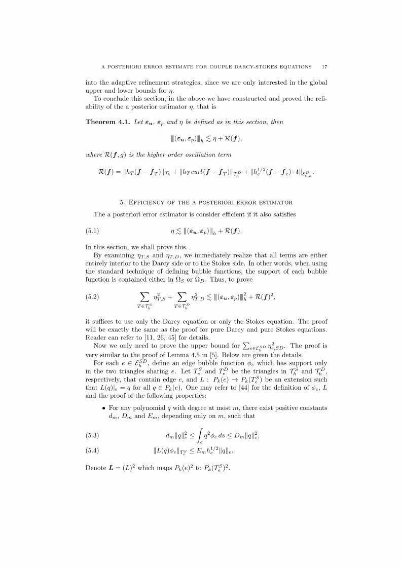
To conclude this section, in the above we have constructed and proved the reli-ability of the a posterior estimator η, that is

Theorem 4.1. Let εu, εp and η be defined as in this section, then

|||(εu, εp)|||h . η +R(f),

where R(f , g) is the higher order oscillation term

R(f) = ‖hT (f − fT )‖Th+ ‖hT curl (f − fT )‖T D

h+ ‖h1/2

e (f − fe) · t‖ED0,h

.

5. Efficiency of the a posteriori error estimator

The a posteriori error estimator is consider efficient if it also satisfies

(5.1) η . |||(εu, εp)|||h +R(f).

In this section, we shall prove this.By examining ηT,S and ηT,D, we immediately realize that all terms are either

entirely interior to the Darcy side or to the Stokes side. In other words, when usingthe standard technique of defining bubble functions, the support of each bubblefunction is contained either in ΩS or ΩD. Thus, to prove

(5.2)∑

T∈T Sh

η2T,S +∑

T∈T Dh

η2T,D . |||(εu, εp)|||2h +R(f)2,

it suffices to use only the Darcy equation or only the Stokes equation. The proofwill be exactly the same as the proof for pure Darcy and pure Stokes equations.Reader can refer to [11, 26, 45] for details.

Now we only need to prove the upper bound for∑

e∈ESDh

η2e,SD. The proof is

very similar to the proof of Lemma 4.5 in [5]. Below are given the details.For each e ∈ ESD

h , define an edge bubble function φe which has support onlyin the two triangles sharing e. Let TS

e and TDe be the triangles in T S

h and T Dh ,

respectively, that contain edge e, and L : Pk(e) → Pk(TSe ) be an extension such

that L(q)|e = q for all q ∈ Pk(e). One may refer to [44] for the definition of φe, Land the proof of the following properties:

• For any polynomial q with degree at most m, there exist positive constantsdm, Dm and Em, depending only on m, such that

dm‖q‖2e ≤

∫

e

q2φe ds ≤ Dm‖q‖2e,(5.3)

‖L(q)φe‖TSe≤ Emh1/2

e ‖q‖e.(5.4)

Denote L = (L)2 which maps Pk(e)2 to Pk(T

Se )2.


Denote χe = T(uh,S , ph,S)n+ph,Dn+µK−1/2(uh,S · t)t on e ∈ ESDh . Then using

(2.6) and (5.3),

‖χe‖2e .

∫

e

χ2eφe ds

=

∫

e

χeφe

(

(T(uh,S , ph,S)− T(uS , pS))n+ (ph,D − pD)n

+ µK−1/2((uh,S − uS) · t)t

)

ds

.

∫

e

χeφe(T(uh,S , ph,S)− T(uS , pS))n ds

+ ‖χe‖e

(

‖ph,D − pD‖e + ‖µK−1/2(uh,S − uS) · t‖e

)

.

Then, using the support of φe, the inverse inequality and Inequality (5.4),∫

e

χeφe(T(uh,S , ph,S)− T(uS , pS))n ds

=

∫

TSe

∇(L(χe)φe)(T(uh,S , ph,S)− T(uS , pS)) dx

+

∫

TSe

L(χe)φe∇ · (T(uh,S , ph,S)− T(uS , pS)) dx

.h1/2e ‖χe‖e

(

h−1TSe‖T(uh,S , ph,S)− T(uS , pS)‖TS

e+ ‖∇ · T(uh,S , ph,S) + f‖TS

e

)

.h−1/2e ‖χe‖e

(

‖∇εu‖TSe+ ‖εp‖TS

e+ ηTS

e ,S + hTSe‖f − fT ‖TS

e

)

.

Using (4.1), we have

‖pD − ph,D‖e

. h−1/2e ‖pD − ph,D‖TD

e+ h1/2

e ‖∇(pD − ph,D)‖TDe

= h−1/2e ‖εp‖TD

e+ h1/2

e ‖f −K−1u−∇ph,D‖TDe

. h−1/2e ‖εp‖TD

e+ h1/2

e ‖f −K−1uh −∇ph,D‖TDe

+ h1/2e ‖K−1(u− uh)‖TD

e

. h−1/2e

(

‖εp‖TDe

+ ηTDe ,D + he‖f − fTD

e‖TD

e+ he‖εu‖TD

e

)

.

Combining the above, using (5.2), the definition of ||| · |||h and R(f), we have

Theorem 5.1. The a posteriori error estimator η satisfies (5.1).

Remark 5.2. In both Theorem 4.1 and 5.1, the constant contained in “.” maydepend on σ, the stabilization parameter in the definition of the bilinear formaS,h(·, ·). However, since σ is of O(1) and does not depend on h, its effect on thestability and efficiency of the a posteriori error estimator η is restricted.

Appendix A. Definition and properties of uh ∈ V h ∩ V

Given uh ∈ V h, here we define uh ∈ V satisfying (4.2). Note that uh is notnecessarily in V h. It is a commonly used technique to introduce such a uh in aposteriori error estimations for nonconforming or discontinuous Galerkin methods.


Readers may refer to [12] and reference therein for similar usage. In [12], uh isconstructed using the Helmholtz decomposition. Here we can not borrow theirresults directly, for two reasons. First, we need an estimation of uh − uh in theV h norm while the construction in [12] only provides a broken H1 semi-normestimation. Second, special treatment needs to be taken in order to ensure that uh

satisfies the interface condition (2.3) strongly.Noticing that in each T ∈ Th, uh is a polynomial with degree less than or equal

to k + 1. Denote Pk+1(Th, S) to be the H1 conforming discrete functional spacewhich consists of piecewise polynomials of degree up to k+1 on each T ∈ Th,S . Wedefine uh as following (as partly illustrated in Figure 3):

(1) uh,S ∈ Pk+1(Th,S)2 is defined by setting its values on all (k + 1)st order

Lagrange interpolation points in T ∈ T Sh . At Lagrange points interior to

any T ∈ T Sh , its value is inherited from the value of uh,S . At Lagrange

points on ΓS , including ΓS ∩ ΓSD, the value is set to be zero. At Lagrangepoints located on edges in ES

0,h∪ESDh but not on ΓS , define the value of uh,S

to be the value of uh,S from a prescribed triangle among all triangles inT Sh sharing this Lagrange point. Note that by such a definition, the values

at Lagrange points on ΓSD are set by using only the Stokes side solutionuh,S .

(2) Now uh,S has been defined. Next, define uh,D in the H(div) conformingRTk+1 space on Th,D by copying the values of uh,D on all degrees of freedomexcept for those associated with e ∈ ESD

h , namely, the degrees of freedomdefined by

∫

e

(uh,D · n)sr ds for all e ∈ ESDh and 0 ≤ r ≤ k + 1.

At these degrees of freedom, to make sure that uh,S · n = uh,D · n on ΓSD,we define

∫

e

(uh,D · n)sr ds =

∫

e

(uh,S · n)sr ds.

Clearly, uh defined as above is in V , but not V h. We have the following lemma:

Lemma A.1. For all T ∈ T Sh ,

(A.1) ‖uh,S − uh,S‖2T + h2

T ‖∇(uh,S − uh,S)‖2T .

∑

e∈ESh(T )

he‖[uh,S ]‖2e,

where ESh (T ) denotes the set of edges in ES

h who have non-empty intersections withT . We especially point out that, benefited from the definition of uh,S, E

Sh (T ) does

not contain edges that lie on ESDh .

Proof. The proof follows from a routine scaling argument and the fact that allnorms on finite dimensional spaces are equivalent. To this end, we observe that

‖uh,S − uh,S‖2T + h2

T ‖∇(uh,S − uh,S)‖2T . h2

T

∑

xj∈Gk(T )

|(uh,S − uh,S)(xj)|2,

where Gk(T ) is the set of all (k + 1)st order Lagrange interpolation points in Tand | · | denotes the Euclidean norm of a vector. It follows from the definition ofuh that uh,S − uh,S vanishes at all internal Lagrange points in T . We only needto examine the value of uh,S − uh,S at Lagrange points on ∂T . There are severaldifferent cases as illustrated in Figure 3.


Figure 3. Setting the values of uh,S at different type of Lagrangepoints on edges. For each Lagrange point, the shaded trianglemeans it is the designated triangle that defines the value of uh,S

on this Lagrange point. On Lagrange points on ΓS , including theintersection of ΓS and ΓSD, the value of uh,S is simply set to bezero.

ΩS

ΩS

ΩS

Γ

SD

Γ

ΓS

ΩD

ΩS

ΩD

SD

Γ

S

ΩS

ΩS

At Lagrange points on edges in ES0,h ∪ ESD

h but not on ΓS , there are two possi-

bilities: (1) xj is in the interior of an edge e; (2) xj is a vertex of T . In the firstcase, we see that |(uh,S − uh,S)(xj)| is either 0 or |[uh,S ]e(xj)|, where [·]e denotesthe jump on edge e, on the two triangles sharing edge e. Furthermore, if xj lies inthe interior of an edge on ΓSD, then |(uh,S − uh,S)(xj)| = 0. In the second case,we can use the triangle inequality to traverse through all edges e ∈ ES

0,h that has

xj as one end point, which we shall denote as e ∈ ESh (xj), and to obtain

(A.2) |(uh,S − uh,S)(xj)| ≤∑

e∈ESh(xj)

|[uh,S ]e(xj)|.

Notice that ESh (xj) does not contain edges in ESD

h . Finally, consider Lagrangepoints on ΓS . Clearly for all xj in the interior of edge e ⊂ ΓS ,

|(uh,S − uh,S)(xj)| = |uh,S(xj)| = |[uh,S ]e(xj)|.

For xj at the end of edge e ⊂ ΓS , again by traversing through all edges e ∈ ES0,h,

we have Inequality (A.2).Combining the above analysis, we have for all T ∈ T S

h∑

xj∈Gk(T )

|(uh,S − uh,S)(xj)|2 .

∑

e∈ESh(T )

∑

xj∈Gk(e)

|[uh,S ]e(xj)|2,

where Gk(e) denotes the corresponding Lagrange points on edge e. Then, using theroutine scaling argument on edges, inequality (A.1) follows immediately.

Using Lemma A.1, inequalities (4.1) and (A.1), we have

‖µ1/2K−1/4(uh,S − uh,S) · t‖2ESDh

.∑

T∈T Sh

(

h−1T ‖uh,S − uh,S‖

2T + hT ‖∇(uh,S − uh,S)‖

2T

)

.‖[uh,S ]‖2ESh

. ‖h−1/2e [uh,S ]‖

2ESh

.


Next, consider the Darcy side. Clearly uh,D − uh,D is only non-zero on triangleswho has at least an edge on ΓSD. Using the definition of uh, the scaling argument,the normal direction continuity on ΓSD, inequalities (4.1) and (A.1), we have onsuch triangles

‖uh,D − uh,D‖2T + h2T ‖∇ · (uh,D − uh,D)‖2T

.∑

e⊂T∩ΓSD

he‖(uh,D − uh,D) · n‖2e

=∑

e⊂T∩ΓSD

he‖(uh,S − uh,S) · n‖2e

.∑

e∈ESh(T )

he‖[uh,S ]‖2e.

Here since T lies on the Darcy side, ESh (T ) means the set of edges in ES

h who hasnon-empty intersection with all triangles in T S

h that shares an edge with T .Combining the above and using the fact that [uh] = 0 on all e ∈ ES

h , thiscompletes the proof of (4.2).

References

1. M. Ainsworth and J.T. Oden, A Posteriori Error Estimators for Stokes and Oseen’s Equa-tions, SIAM J. Numer. Anal., 17 (1997), 228–246.

2. A. Alonso, Error estimators for a mixed method, Numer. Math., 74 (1996), 385–395.3. T. Arbogast and D.S. Brunson, A computational method for approximating a Darcy-Stokes

system governing a vuggy porous medium, Computational Geosciences, 11 (2007), 207–218.4. D.N. Arnold, L.R. Scott and M. Vogelius, Regular inversion of the divergence operator with

Dirichlet boundary conditions on a polygon, Ann. Scuola Norm. Sup. Pisa Cl. Sci. (4), 15(1988), 169–192.

5. I. Babuska and G. N. Gatica, A residual-based a posteriori error estimator for the Stokes-

Darcy coupled problem, SIAM J. Numer. Anal. 48 (2010), 498–523.6. R. Bank and B. Welfert, A Posteriori Error Estimates for the Stokes Problem, SIAM J.

Numer. Anal., 28 (1991), 591–623.7. G.S. Beavers and D.D. Joseph, Boundary conditions at a naturally permeable wall, J. Fluid

Mech., 30 (1967), 197–207.8. D. Braess and R. Verfurth, A posteriori error estimators for the Raviart-Thomas element,

SIAM J. Numer. Anal., 33 (1996), 2431–2444.

9. F. Brezzi, J. Douglas, and L. Marini, Two families of mixed finite elements for second orderelliptic problem, Numer. Math., 47 (1985), 217–235.

10. F. Brezzi and M. Fortin, Mixed and Hybrid Finite Elements, Springer-Verlag, New York, 1991.11. C. Carstensen, A posteriori error estimate for the mixed finite element method, Math. Comp.,

66 (1997), 465–476.12. C. Carstensen and J. Hu, A unifying theory of a posteriori error control for nonconforming

finite element methods, Numer. Math., 107 (2007), 473–502.13. C. Carstensen, T. Gudi, M. Jensen, A Unifying Theory of A Posteriori Control for Discon-

tinuous Galerkin FEM, Numer. Math., 112 (2009), 363–379.14. Z. Chen, Finite Element Methods and Their Applications, Springer-Verlag, Berlin Heidelberg,

2005.

15. B. Cockburn, G. Kanschat, and D. Schotzau, A locally conservative LDG method for theincompressible Navier-Stokes equations, Math. Comput., 74 (2005), 1067–1095.

16. B. Cockburn, G. Kanschat, and D. Schotzau, A note on discontinuous Galerkin divergence-free solutions of the Navier-Stokes equations, J. Sci. Comput., 31 (2007), 61–73.

17. M. Cui and N. Yan, A posteriori error estimate for the Stokes-Darcy system, Math. Meth.Appl. Sci., 34 (2011), 1050–1064.

18. E. Dari, R. G. Duran and C. Padra, Error estimators for nonconforming finite element

approximations of the Stokes problem, Math. Comp., 64 (1995), 1017–1033.


19. M. Discacciati and A. Quarteroni, Navier-Stokes/Darcy Coupling: Modeling, Analysis, andNumerical Approximation, Rev. Mat. Complut., 22 (2009), 315–426.

20. W. Doerfler and M. Ainsworth, Reliable a posteriori error control for non-conforming finiteelement approximation of Stokes flow, Math. Comp., 74 (2005), 1599–1619.

21. J. Galvis and M. Sarkis, Non-matching mortar discretization analysis for the coupling Stokes-Darcy equations, Electon. Trans. Numer. Anal., 26 (2007), 350–384.

22. G.N. Gatica, S. Meddahi and R. Oyarzua, A conforming mixed finite-element method for thecoupling of fluid flow with porous media flow, IMA J. Numer. Anal., 29 (2009), 86–108.

23. G.N. Gatica, R. Oyarzua and F.-J. Sayas, Convergence of a family of Galerkin discretizationsfor the Stokes-Darcy coupled problem, Numer. Meth. Part. Diff. Eq., 27 (2011), 721–748.

24. V. Girault, G. Kanschat and B. Riviere, Error analysis for a monolithic discretization ofcoupled Darcy and Stokes problems, preprint.

25. V. Girault and B. Riviere, DG approximation of coupled Navier-Stokes and Darcy equations

by Beaver-Joseph-Saffman interface condition, SIAM J. Numer. Anal., 47 (2009), 2052–2089.26. A. Hannukainen, R. Stenberg and M. Vohralik, A unified framework for a posteriori error

estimation for the Stokes problem, Numer. Math., submitted.27. W. Jager and A. Mikelic, On the boundary conditions at the contact interface between a

porous medium and a free fluid, Ann. Scuola Norm. Sup. Pisa Cl. Sci., 23 (1996), 403–465.28. W. Jager and A. Mikelic, On the interface boundary condition of Beavers, Joseph and

Saffman, SIAM J. Appl. Math., 60 (2000), 1111–1127.

29. W. Jager, A. Mikelic and N. Neuss, Asymptotic analysis of the laminar viscous flow over aporous bed, SIAM J. Sci. Comput., 22 (2001), 2006–2028.

30. G. Kanschat and B. Riviere, A strongly conservative finite element method for the couplingof Stokes and Darcy flow, J. Comput. Phys., 229 (2010), 5933–5943.

31. T. Karper, K.-A. Mardal and R. Winther, Unified Finite Element Discretizations of CoupledDarcyCStokes Flow Numer. Meth. Part. Diff. Eq., 25 (2008), 311–326.

32. W.J. Layton, F. Schieweck and I. Yotov, Coupling fluid flow with porous media flow, SIAMJ. Numer. Anal., 40 (2003), 2195–2218.

33. J. L. Lions and E. Magenes, Non-homogeneous Boundary Value Problems and Applications,Vol. 1, Springer-Verlag, New York-Heidelberg, 1972.

34. C. Lovadina and R. Stenberg, Energy norm a posteriori error estimates for mixed finite

element methods, Math. Comp., 75 (2006), 1659–1674.35. F. Nobile, A posteriori error estimates for the finite element approximation of the Stokes

problem, TICAM Report 03-13, April 2003.36. L.E. Payne and B. Straughan, Analysis of the boundary condition at the interface between

a viscous fluid and a porous medium and related modelling questions, J. Math. Pures Appl.,77 (1998), 317–354.

37. P.A. Raviart and J.M. Thomas, A mixed finite element method for second order elliptic

problems, Mathematical aspects of the finite element method, Eds. I. Galligani andE. Magenes, Lecture notes in Mathematics, Vol. 606., Springer-Verlag, 1977.

38. B. Riviere, Analysis of a Discontinuous Finite Element Method for the Coupled Stokes andDarcy Problems, J. Sci. Comp., 22-23 (2005), 479–500.

39. B. Riviere and I. Yotov, Locally conservative coupling of Stokes and Darcy flows, SIAM JNumer. Anal., 42 (2005), 1959–1977.

40. P.G. Saffman, On the boundary condition at the interface of a porous medium, Stud. Appl.Math., 1 (1971), 93–101.

41. L. R. Scott and S. Zhang. Finite element interpolation of nonsmooth function satisfyingboundary conditions, Math. Comp., 54 (1990), 483–493.

42. R. Verfurth, A posteriori error estimators for the Stokes equations, Numer. Math., 3

(1989), 309–325.43. R. Verfurth, A posteriori error estimators for the Stokes equations II. Non-conforming

discretizations, Numer. Math., 60 (1991), 235–249.44. R. Verfurth, A review of a posteriori error estimation and adaptive mesh-refinement tech-

niques. Teubner Skripten zur Numerik. B.G. Willey-Teubner, Stuttgart, 1996.45. J. Wang, Y. Wang and X. Ye, A posteriori error estimation for an interior penalty type

method employing H(div) Elements for the Stokes equations, SIAM J. Sci. Comp., 33 (2011),

131–152.


46. J. Wang, Y. Wang and X. Ye, A posteriori error estimate for stabilized finite elementmethods for the Stokes equations, Int. J. Numer. Anal. Model., 9 (2012), 1–16.

47. J. Wang and X. Ye, New finite element methods in computational fluid dynamics by H(div)elements, SIAM J. Numer. Anal., 45 (2007), 1269–1286.

School of Mathematics, Fudan University, Shanghai, ChinaE-mail address: [email protected]

Department of Mathematics, Oklahoma State University, Stillwater, OK, USA

E-mail address: [email protected]

A POSTERIORI ERROR ESTIMATE FOR THE CONFORMING …...A POSTERIORI ERROR ESTIMATE FOR THE H(div)...

Documents

Transcript of A POSTERIORI ERROR ESTIMATE FOR THE CONFORMING …...A POSTERIORI ERROR ESTIMATE FOR THE H(div)...