A polyhedral approach to the discrete lot-sizing and ... · A Polyhedral Approach to the Discrete...
128
A polyhedral approach to the discrete lot-sizing and scheduling problem van Eijl, C.A. DOI: 10.6100/IR461120 Published: 01/01/1996 Document Version Publisher’s PDF, also known as Version of Record (includes final page, issue and volume numbers) Please check the document version of this publication: • A submitted manuscript is the author's version of the article upon submission and before peer-review. There can be important differences between the submitted version and the official published version of record. People interested in the research are advised to contact the author for the final version of the publication, or visit the DOI to the publisher's website. • The final author version and the galley proof are versions of the publication after peer review. • The final published version features the final layout of the paper including the volume, issue and page numbers. Link to publication General rights Copyright and moral rights for the publications made accessible in the public portal are retained by the authors and/or other copyright owners and it is a condition of accessing publications that users recognise and abide by the legal requirements associated with these rights. • Users may download and print one copy of any publication from the public portal for the purpose of private study or research. • You may not further distribute the material or use it for any profit-making activity or commercial gain • You may freely distribute the URL identifying the publication in the public portal ? Take down policy If you believe that this document breaches copyright please contact us providing details, and we will remove access to the work immediately and investigate your claim. Download date: 16. Jul. 2018
-
Upload
vuongnguyet -
Category
Documents
-
view
239 -
download
0
Transcript of A polyhedral approach to the discrete lot-sizing and ... · A Polyhedral Approach to the Discrete...

A polyhedral approach to the discrete lot-sizing andscheduling problemvan Eijl, C.A.
DOI:10.6100/IR461120
Published: 01/01/1996
Document VersionPublisher’s PDF, also known as Version of Record (includes final page, issue and volume numbers)
Please check the document version of this publication:
• A submitted manuscript is the author's version of the article upon submission and before peer-review. There can be important differencesbetween the submitted version and the official published version of record. People interested in the research are advised to contact theauthor for the final version of the publication, or visit the DOI to the publisher's website.• The final author version and the galley proof are versions of the publication after peer review.• The final published version features the final layout of the paper including the volume, issue and page numbers.
Link to publication
General rightsCopyright and moral rights for the publications made accessible in the public portal are retained by the authors and/or other copyright ownersand it is a condition of accessing publications that users recognise and abide by the legal requirements associated with these rights.
• Users may download and print one copy of any publication from the public portal for the purpose of private study or research. • You may not further distribute the material or use it for any profit-making activity or commercial gain • You may freely distribute the URL identifying the publication in the public portal ?
Take down policyIf you believe that this document breaches copyright please contact us providing details, and we will remove access to the work immediatelyand investigate your claim.
Download date: 16. Jul. 2018

A Polyhedral Approach to the
Discrete Lot-sizing and Scheduling Problem
Cleola van Eijl

A Polyhedral Approach to the
Discrete Lot-sizing and Scheduling Problem
PROEFSCHRIFT'
ter verkrijging van de graad van doctor aan de Technische Universiteit Eindhoven, op gezag van de Rector Magnificus, prof. dr. J .H. van Lint, voor een commissie aangewezen door het College van Dekanen in het openbaar te verdedigen op
vrijdag 14juni 1996om 16.00 uur
door
CLEOLA ANGELINA VAN EIJL
geboren te Terneuzen

Dit proefschrift is goedgekeurd door de promotoren:
prof.dr. J.K. Lenstra en prof.dr. Y. Pochet
Copromotor: dr.ir. C.P.M. van Hoesel
Druk: Boek- en Offsetdrukkerij Letru, Helmond, (0492) 53 77 97

Contents
1 Introduetion 3
1.1 Polyhedral combinatorics 3 1.2 The discrete lot-sizing and scheduling problem 6 1.3 Outline of the thesis 10
2 The single-item DLSP 12 2.1 Preliminaries 12 2.2 Pacet-defining inequalities 14
2.2.1 General farm 14 2.2.2 Hole-lifted right stock-minimal inequalities 21 2.2.3 Regular block inequalities 33 2.2.4 Hole-lifted left stock-minimal inequalities 43 2.2.5 Further remarks 51
2.3 Wagner-Whitin costs 52
3 The multi-item DLSP 61 3.1 Complexity 61 3.2 Valid inequalities 65
3.2.1 Single-item inequalities 65 3.2.2 Multi-item inequalities 67
3.3 Branch-and-cut 69 3.3.1 Implementation issues 69 3.3.2 Computational results 72
3.4 Related research 78
4 Sequence-independent startop times 81 4.1 Pormulation 81 4.2 Valid inequalities 83 4.3 A multicommodity flow formulation 89
s The delivery man problem 95 5.1 Pormulation 95 5.2 Valid inequalities 97
5.2.1 Inequalities for the delivery man problem 98 5.2.2 Inequalities for the delivery man problem with time windows 103

2
5.3 Computational experiments 5.3.1 Implementation issues 5.3.2 Results 5.3.3 Further remarks
Bibliography
Samenvatting
Acknowledgements
Contents
105 105 106 109
111
115
118

1. Introduetion
For several decades such divergent areas as production planning, transportation, telecommunication, and VLSI design have been an inexhaustible souree of combinatorial optimization problems. These problems are usually characterized by a finite set of solutions from which the best solution with respecttoa given objective function has to be found. The practical relevanee of many combinatorial optimization problems stimulates the search for good solution methods. Unfortunately, most of these problems are NP-hard (cf. Garey and Johnson [16]). This implies that it is generally considered to be very unlikely that efficient solution methocts for such problems willever be developed. As a consequence, a vast amount of research in combinatorial optimization is devoted to the design of approximation algorithms that find reasonably good solutions in an acceptable amount of time. Nevertheless, algorithms that always provide the optimal solution but for which an efficient performance cannot be guaranteed, have also proven to be of great use in tackling hard combinatorial optimization problems. An optimization technique that bas contributed to the successful solution of a large number of these problems, as for example listed by Jünger et al. [23] and Aardal and van Hoesel [1], is based on polyhedral combinatorics. InSection 1.1 we present basic concepts and results from polyhedral theory and discusshow polyhedral techniques can be applied in order to solve problems in the area of combinatorial optimization.
In this thesis we study the discrete lot-sizing and scheduling problem from a polyhedral point of view. This problem is one of the many lot-sizing models, which have been classified in a recent paper by Kuik et al. [24]. This paperalso gives an extensive survey ofthe research in this area. The usual setting fora lot-sizing problem is a production facility that can produce several different items. One bas to delermine at what time and in what amount the items have to be produced in order to meet a given demand at minimum costs. Basic in lot-sizing is the trade-offbetween the costs related to inventory and the costs incurred by adjusting the facility for the production of a particular item. The typical features of the discrete lot-sizing and scheduling problem will be discussed inSection 1.2. This sectionis further devoted to the modeling of the problem and a review of earlierresearch on the subject.
An outline of the remainder of the thesis concludes this chapter.
1.1 Polyhedral combinatorics
In this section we will discusshow polyhedral methods can be applied to solve combinatorial optimization problems. First somebasic concepts and results from polyhedral theory are introduced. For a detailed treatment of this subject, including proofs of the results stated bere, the reader is referred to Nemhauser and Wolsey [30] and Schrijver [39].
4 Introduetion
For many combinatorial optirnization problems, the solutions can be represented as n-dimensional integral veetors x that satisfy a set of linear constraints and for which the objective function is linear in the variables X;, 1 ~ i ~ n. Such a problem can thus be formulated as
min{cx: Ax ~ b, x EZ"}, (1.1)
i.e., for given c, A, and b we have to find the integral vector x satisfying Ax ::; b with minimum cost ex. Here c, A, and bare assumed to be integral. This formulation is called an integer linear programming problem, or lP for short. If only a subset of the variables has to be integral, then the problem is called a mixed integer linear programming problem (MIP). In the remainder we will only consider IPs, but the results hold for MIPs as well.
In this context an algorithm is said to be efficient if it solves every instanee of a problem to optimality in a number of steps that is polynomial in the size of the input. The NP-hardness
of most combinatorial optimization problems suggests that an efficient metbod for solvingIPs is not likely to be ever developed. The integrality constraints form the complicating factor. If these constraints are ornitted from the formulation, then the resulting problem is a linear programming problem (LP), called the linear programming relaxation or LP-relaxation of the lP under consideration. LPs are in general considerably easier than IPs, since they can be solved in polynomial time.
In order to obtain a solution to the lP one can apply branch-and-bound. This is a general impHeit enumeration technique to solve combinatorial optimization problems. Here we restriet ourselves to the description of a linear programming based branch-and-bound procedure. In such a solution approach the original lP is partitioned into several subproblems by adding linear constraints. For example, in case of binary variables two subproblems can be created by fixing one variabie to zero and one, respectively. For each subproblem we sol ve the
corresponding LP-relaxation. If the linear program is infeasible or if its solution is integral, then the subproblem needs no further evaluation. Otherwise, a further refinement is made by splitting the subproblem into new subproblems. Note that the LP-relaxation provides a lower bound to the optimal value of the subproblem. If this lower bound is greater than or equal to the value of the currently best solution to the original problem, then the subproblem can also be discarded from further evaluation. Hence, in order to keep the number of subproblems that bas to be evaluated as small as possible, it is important that strong lower bounds can be computed in an efficient way. Our efforts in applying polyhedral techniques are aimed at finding a strong LP-formulation of the problem at hand that serves as a good starting point for the
branch-and-bound procedure.
Basic in polyhedral combinatodes is the existence of a linear program min{cx: A' x ::; b'} that solves the integer program ( 1.1). Before we state the two results from which this is an immediate consequence, we fust introducesome terrninology. Let S = {x1, ... , xk} be a set
of veetors in ~~~. The convexhullof S, denoted by conv(S), is the set o::::~=l À;Xî : L~=l À; = 1 and À; 2:0 for all i}. Thefirstresultis thatmin{cx: x ES}= min{cx: x E conv(S)} for any

1.1 Polyhedral combinatorics 5
linear function c. Second, the convex huil of a fini te numher of points is a bounded polyhedron, i.e., thereexistsafiniteset oflinear inequalities Ax s b such thatconv(S) ={x E IRn: Ax s b}. We say that Ax s bis a linear de scription of conv(S).
From the aforementioned it follows that the combinatorial optimization problem (1.1) can besolved by solving thelinearprogrammin{cx: A' x s b'}, whereA'x s b' is alineardescription of the convex huil of thesetof feasible solutions S ={x: Ax s b, x integral}. For most problems, however, it is very hard to find a complete linear description of conv(S). One therefore usually restricts oneself to the derivation of one or more classes of valid inequalities for the convexhullof S. These are inequalities that are satisfied by allelementsof S. In particular, one is interested in the so-calledfacet-defining inequalities, which are necessary in the linear description of conv(S). Before we explain the latter term, some more definitions are introduced. Consicter a polyhedron P = {x E IRn : Ax s b} and let ax s {3 be a valid inequality for P. The set F = {x E P : ax = {3} is called a face of P and ax s {3 is said to define F. If F is neither empty nor equal toP, then it is said to he a proper face of P. A vector x is called a direction of P if there exist two different veetors x1 and x2 in P such that x = x1
- x2 • Moreover, a set of veetors x1 , ••• , x* is said to he linearly independent if .L:L À;xi = 0 implies that À; = 0 for all i. The dimension of a polyhedron P, denoted by dim(P}, is defined as the maximum numher of linearly independent directionsin P. lf dim(P) n, then P is said to he full-dimensional. This only occurs if there is no inequality that is satisfied at equality by all x E P. Note that a face of a polyhedron is also a polyhedron. Now thefacets of a polyhedron P are those faces F with dim( F) dim( P) 1. Together with the equalities that are satisfied by all x E P, the facet-defining inequalities yield a linear description of P with as few constraints as possible. In order to prove that a valid inequality ax s {3 for a polyhedron P defines a facet, we proceed as follows. First, we have to show that there is a vector x0 E P such that ax0 < {3. This is usually trivialand therefore not explicitly mentioned. Then we provide dim(P) llinearly independent directionsx1 - x2 , wherex1 and x2 are twodifferent veetors in P that satisfy the inequality at equality.
Suppose that for the integer program (1.1) a partiallinear description of the convex hull of thesetof feasible solutions bas been established. An explicit list of all inequalities, even when restricted to those that are facet-defining, usually yields a linear program that is too large to he handled by any LP-solver. However, in order to find the optima! solution to the lP, it suffices to include only a small numher of inequalities, namely, the facet-defining inequalities that are satisfied at equality by this solution. This observation suggests the following procedure for solving IPs:
1. Take the LP-relaxation min{cx: Ax s b} as the first linear program. Go to 2. 2. Solve the current LP and denote the optima! solution by x. lf x is integral,
then stop; otherwise go to 3. 3. Find a valid inequality that is violated by x. If no such inequality can be found,
then stop; otherwise add the inequality to the LP and go to 2.
6 Introduetion
This is called a cutting plane algorithm, since the inequalities found in Step 2 cut offthe current LP-solution. The procedure of finding violated inequalities is called separation. A separation algorithm for a class of valid inequalities is called exnct if it always fincts a violated inequality in this class unless such an inequality does not exist. When no reasonably fast exact separation procedure is known, one usually applies a heuristic method. Then it is not guaranteed that there are no violated inequalities in the class at hand if the algorithm fails to find one.
The cutting plane algorithm terminates in one of the following two ways: either an integral solution is obtained in Step 2, or no violated inequality is identified in Step 3. In the fust case, we have found an optimal solution to the lP. In the latter case, i is fractional and ei is a lower bound to the optimal value of the lP. Then an optimal integral solution can be obtained by applying branch-and-bound. In the branch-and-bound procedure one can try to improve the lower bounds by subjecting the subproblems to the cutting plane procedure. The combination of branch-and-bound and cutting planes is called branch-and-cut. Apart from good separation algorithms, the performance of a branch-anct-eut algorithm depends on many other aspects such as the definition ofthe subproblems and the availability of strong upper bounds. Implementation issues in branch-and-cut algorithms are extensively discussed by Jünger et al. [23].
1.2 The discrete lot-sizing and scheduling problem
The main subject of our research is the discrete lot-sizing and scheduling problem, or DLSP for short. This production planning problem is concerned with a single machine that can produce a number of different items. The planning horizon is partitioned into small periods in each of which production occurs for at most one item. Furthermore, we assume an all-arnothing policy with respect to the production level in one period, i.e., the production is either zero or at full capacity, which is defined as one unit of one item. This is often a reasonable assumption in short-term production planning, when the time periods are smalt. The demand for each item is dynamîc and bas to be satisfied without backlogging. In the fust period of a production batch a so-called startup cost is incurred for setting up the machine for the item at hand. Since in multi-item problems startup costs usually arise when the machine switches from the production of one item to the production of another item, these costs arealso known as changeover costs. Apart from startup costs, production and inventory costs have tobetaken into account. Now DLSP is the problem of determining a production schedule that satisfies the given restrictions at m:inimum costs.
Startup costs are said to besequence-independentifthey only depend on the item for which the machine is set up. DLSP with sequence-independent stmtup costs is studied in Chapters 2 and 3. Moreover, a startup is assumed not to affect the production capacity. This assumption is reasonable, e.g., when the startups occur out of regular production hours. In Chapter 4 we consicter an extension of DLSP in which startups take up an integral number of production periods.

1.2 The discrete lot-sizing and scheduling problem 7
In practice planning problems will usually have more complicating features than the on es captured by DLSP. Nevertheless, the study of these simplified modelsis a valuable aidin the solution of more realistic problems. Case-studies of production planning systems in which DLSP appears as a subproblem are presented by Van Wassenhave and Vanderhen st [40] and de Lange [25]. In the first paper only single-item problems have to be solved, whereas de Lange considers DLSP with sequence-dependent startup times. Moreover, Fleischmann [14] showshow DLSP can be used as an approximation for a capacitated lot-sizing problem with larger time periods in which production can occur for more than one item.
From the NP-hardness of DLSP (cf. Chapter 3) it follows that one should not strive for a polynomial-time solution procedure. Salomon [35] presents a dynamic programming algorithm for solving DLSP with sequence-independent casts. The running time of this algorithm is O(M2TTI:!1 D;), where M denotes thenumber of items, T thenumber ofperiods, and D;
the total de mand for item i. Thus, when the number of items is fixed the problem can be solved in polynomial time. In particular, the single-item DLSP can be solved in O(T D) time, where D denotes the total demand. For special co st functions faster algorithms are developed by van Hoesel [18] (see also [21]).
The dynamic programming algorithm for the single-item DLSP plays an important role in two other approaches to DLSP with sequence-independent startup costs, namely, by Lagrangean relaxation (Fleischmann [14]) and column generation (Cattrysse et al. [7]). An outline of bath solution methods will be given in Chapter 3. The latter approach was in fact primarily developed for DLSP with sequence-independent startup times. In order to handle sequence-dependent startup costs Fleischmann [15] reformulates DLSP as a traveling salesman problem with additional time constraints and proposes a salution procedure in which lower bounds are obtained by Lagrangean relaxation. We return to this reformulation at the end of the section. Salution methods for DLSP with sequence-dependent startup times are discussed in recent papers by Salomon et al. [37] and Jordan and Drexl [22]. The former authors present an approachbasedon dynamic programming, whereas Jordan and Drexl transfarm the problem into a batch sequencing problem which is solved by a branch-and-bound algorithm.
The remainder of this sectionis mainly devoted to DLSP with sequence-independent startup costs. First an integer linear programming formulation ofthe problem is discussed. Then we will review polyhedral results that are obtained for DLSP and some generalizations. For a comprehensive survey of results for lot-sizing problems in the area of polyhedral combinatodes we refer to Pochet and Wolsey [33].
Let T denote the number ofperiods and let M denote the number of items. The demand for item i in period t is denoted by d:. Since at most one unit of one item is produced per period, we assume withoutlossof generality that d: E {0, 1} for all i and t. Furthermore, let p: denote the cost for producing item i in period t, h; the costof holding one unit of item i in stock at the end of period t, and Jj the startup co st that is incurred when the machine is set up in period t for the production of item i.
The problem can be mathematically formulated using two types of binary variables: x~,

8 Introduetion
which indicates whether production occurs for item i in period t or not, and y;, which takes the value one if a startup occurs for item i in period tand zero otherwise. For notational con
venience we write xL2 insteadof 2::~11 x:, dt.rz insteadof 2::~ 1, d;, etc .. If M = 1, then the superscript i will be omitted.
We assume thatinitial inventories are zero. Consequently, the inventory of item i at the end ofperiod t equals the total production of item i up to period t minus the total demand of item i up to this period. Hence, the inventory costs for item i can be expressedas h: (x~
1- df
1).
Define c; P! + h!,r and Hi = - 2:;=1 h;dL. Now DLSP can be modeled as ' ,
M T (DLSP) min.L:.L:<c:x: + J/y:)
i'=1 1=1
s.t. xL :::: dL (1 ::; i ::; M, 1 ::; t ::; T) (1.2}
xi < xi +Yi r- r-1 t (1::; i::; M, 1::; t::; T, x&= 0) (1.3) M
z:::x: ::; 1 (1::; t::; T) (1.4) i=1
x;, Yl E {0, 1} (1 ::; i::; M, 1 ::; t::; T) (1.5)
where the constant 2::!1 Hi is omitted from the objective function. Constraints (1.2) imply that for item i the total production up to period t is at least equal to the total demand up to this period. Inequalities (1.3) force that a startup for item i takes place in period t if production occurs for item i in this period, but not in the preceding one. Constraints ( 1.4) are the coupling constraints which state that in any period production can occur for only one item. Observe that when these constraints are not taken into account, the remaining problem consists of M single-item problems.
Note that a solution to (1.2) - ( 1.5) may have a positive inventory at the end of the planning horizon. Moreover, a startup is allowed to occur in a period without production, i.e., we may have y; = 1 and x; 0 forsome item i and period t. Also solutions in which two batches of the sameitem are scheduled contiguously, i.e., solutions with x;_1 = Y! x; 1 forsome i and t are allowed. One can easily add extra constraints to the model in order to exclude solutions having one of the aforementioned features. However, such a solution is never optimal when all costs are positive.
Polyhedral results for lot-sizing problems mainly concern the polyhedral structure of singleitem models (cf. [33]). This also holds for the results described in this thesis. Obviously, valid inequalities for the single-item formulation remain valid for the multi-item problem.
For the single-item DLSP van Hoesel [18] characterizes one class of facet-defining inequalities, the so-called hole-bucket inequalities. A polynomial separation algorithm forthese inequalities is given in [19]. Van Hoesel and Kolen present a multicommodity flow reformulation of the single-item DLSP in [20]. This model is obtained by splitting the original production variabie x1 intovariables Xrk which have value one if the production in period t satisfies the

1.2 The discrete lot-sizing and scheduling problem 9
demand in the kth demand period and zero otherwise. For this tormulation a complete linear description of the associated polyhedron is derived. No te that such a tormulation bas a bout
dt,T T variables, whereas the original tormulation bas only 2T variables.
DLSP can be considered as a special case of the capacitated lot-sizing problem with stanup casts or CLSS for short. We discuss bere the single-item version of this problem. In CLSS the
production in period t can attain any value between zero and the available capacity C1• The amount of production in period t is denoted by X1 and incurs a cost c1X1• The binary setup
variabie Y1 indicates whether production can take place in period t or not. Obviously, Y1 must be one if X1 > 0. However, the machine might be set up for production, even if no production occurs. The setup cost ft can be considered as the fixed co st incurred whenever the machine is able to produce, Moreover, if the machine is set up in a period t, but not in the preceding period, then a startup bas to occur in period t. The startup variables and startup costs are bere denoted by Z1 and g~> respectively. Now CLSS can be formulated as
(CLSS)
s.t.
T
min L(c1X1 + /1f1 + g1Z1) 1=1
X1,1 ?: d1,1
Y1 ~ Y1-1 + Z1
XI ~ CIYI
X1?: 0, Yr, Z1 E {0, 1}
(1 ~ t ~ T)
(1 ~ t ~ T, Yo = 0)
(1 ~ t ~ T)
(1 ~ t ~ T)
CLSS clearlyreduces to DLSP ifwe set C1 equal to oneandrequire X1 = Yr forevery t. Hence, valid inequalities for CLSS can be easily turned into valid inequalities for DLSP. However, even if the original inequality is facet-defining for CLSS, the resulting inequality might be
trivia! ordefine a face of low dimension for DLSP. Constantino [5] derives several classes of valid inequalities for CLSS. In relation to our
work two classes are of great importance, namely, the left and right supermodular inequalities. The ideas bebind these inequalities will be discussed in Chapter 2. For two subclasses,
the intervalleft and right supennodular inequalities, Constantino establishes necessary and sufficient conditions for an inequality to be facet-defining and gives a polynomial-time separation algorithm. Moreover, he introduces valid inequalities for the single-item problem with more complicating features, such as lower bounds on the production and backlogging, and two classes of multi-item inequalities.
Magnanti and V achani [28] and Sastry [38] study the special case of CLSS in which C1 = 1 for every t and the production variables are also binary. Hence, the only difference with DLSP is that the setup of the machine can be maintained during idle periods. In this way, one can avoid a more expensive startup. A class of facet-defining inequalities for this problem is discussed in [28]. This class forms the basis of the skip inequalities introduced by Sastry. He
gives a complete characterization of facet-defining skip inequalities and presents a separation
algorithm based on linear programming for one subclass. For some problems it can be shown that a partiallinear description of the related polyhe-

10 Introduetion
dron always provides an optimal salution with respect to a certain class of objective functions. For lot-sizing problems this kind of result bas been obtained for cost functions that satisfy the Wagner-Whitin property. For DLSP a cost function is said to be of the Wagner-Whitin type if the unit inventory cost hr and the production cost Pr satisfy h, + Pt 2: Pt+I for every period t. Recalling that Cr = p, + h1,r, this is easily seen to be equivalent to c1 2: ct+1 for all t. The Wagner-Whitin property implies that it is always optimal to produce as late as possible. Hence, with Wagner-Whitin costs there always exists an optimal salution for which the inventory at the end of period t - 1 is zero for any period t in which a production batch is started. Pochet and Wolsey [32] study four single-item lot-sizing problems and give for each of them a partiallinear description of the convex huil that solves the problem in the presence ofWagner-Whitin costs. These polyhedra involve considerably fewer constraints than in the general cost case. In Section 2.3 we derive a similar result for the single-item DLSP.
We conclude this section with a brief discussion of the reformulation of DLSP as a traveling salesman problem with time windows (TSVIW). Consicter a graph in which every unit of demand is represented by a node, i.e., if d; = 1, then this unit of demand is represented by a node v(i, t). With v(i, t) a deadline t is associated. Now a production schedule can be considered as a tour that starts and finishes at a depot and visits every node before or at its deadline. The travel time between two nodes equals one if the nodes correspond to units of the same item, and one plus the required startup time otherwise. Startup and production costs are incorporated in the costs of using an are, whereas inventory costs can be modeled as costs incurred when a node is visited strictly before its deadline.
Reischmann [15] was the first to formulate DLSP as a TSP'IW. He models DLSP with sequence-dependent startup costs and zero startup times as a TSVIW with time-dependent costs. A reformulation of DLSP with sequence-dependent startup times as a TSPTW is presented by Salomon et al. [37). Both problems will not be considered in this thesis. However, in Chapter 5 we will study another variant of the TSP, the so-called delivery man problem, in which the objective is to find a tourstarting from a given depot that minimizes the sum of the waiting times of the customers located at the nodes. We will present a MIP-formulation that can easily be turned into a formulation for the TSVIW. Furthermore, we will derive some additional valid inequalities and report computational results.
1.3 Outline of the thesis
The remainder of the thesis is organized as follows. Chapters 2 and 3 are devoted to the discrete lot-sizing and scheduling problem with se
quence-independentstartup costs. In Chapter 2 we study the polyhedral structure of the singleitem version ofthe formulation discussed in the previous section. We first investigate the general form of facet-defining inequalities for which all coefficients of the x-variables are either zero or one. Then three subclasses are discussed in more detail. In the last section we present

1.3 Outline of the thesis 11
a partiallinear description of the convex hull of feasible solutions that solves the problem in the presence ofWagner-Whitin costs. This result already appeared in van Eijl and van Hoesel [11]. The multi-item problem is dealt with in Chapter 3. lts computational complexity is addressed first. Furthermore, we describe the implementation of a branch-and-cut algorithm andreport computational results.
In Chapter 4 the problem with sequence-independen tstartup times is considered. We show that this problem can be modeled by a slight modification of the tormulation for the problem that only involves startup costs. Valid inequalities for the latter tormulation are hence easily turned into valid inequalities for the problem with startup times. We also present a multicommodity flow tormulation for the single-item problem and show that its LP-relaxation solves the problem to optimality.
As mentioned before, Chapter 5 differs from the other chapters in that it focuses on the delivery man problem instead of the discrete lot-sizing and scheduling problem. We present a mixed integer programming tormulation for this problem, derive classes of additional valid inequalities, and give some computational results. This chapter is basedon van Eijl [10].

2. The single-item DLSP
In this chapter we study the pol yhedral structure of the model discussed in the previous chapter when only one item is involved. Although the single-itemDLSP is polynomially solvable, an explicit description of the convex hull of the set of feasible solutions to this tormulation is not known. A partiallinear description is given by van Hoesel [18]. Magnanti and Vachani [28] and Sastry [38] derive inequalities for a slightly more general problem in which also setup costs are involved. Furthermore, Constantino [5] derives several classes of valid inequalities for the capacitated lot-sizing problem with startup costs. This problem is a generalization of DLSP in which the production in period t can attain any value between zero and the available capacity in this period. Inequalîties forthese more general problems can easily be adapted to valid inequalities for DLSP. However, even if we start from a facet-defining inequality for the original problem, the resulting inequality for DLSP might be trivial or define a face of low dimension.
This chapter is organized as follows. In Section 2.1 the formulation from Chapter 1 is reviewed. In Section 2.2 we fust investigate the general form of facet-defining inequalities for which all coefficients of the x-variables are either zero or one. Then three subclasses are discussed in more detail. The first subclass slightly extends the class of right supermodular inequalities of Constantino when adapted to DLSP. The inequalities of the first subclass are also related to the skip inequalities discussed in [38]. The second subclass generalizes the hole-bucket inequalities introduced by van Hoesel. The lastsubclassis again an extension of a class derived by Constantino, namely, the class of intervalleft supermodular inequalities. For all three subclasses we also address the separation problem. Inthelast section we present a partiallinear description of the convex huil of feasible solutions that solves the problem in the presence ofWagner-Whitin costs.
2.1 Preliminaries
Throughout, the interval {tt, ... , tz} ~ {1, ... , T} will be denoted by [tt, tz]. If ft > tz, then [t1, t2] 0. Now the single-item version of the model discussed in the previous chapter reacts
as follows: T
(DLSP) min 2)c:Xz + frYz) 1=1
s.t. Xt,: 2: de: for all t E [1, T] (2.1)
Xt ::::; X:-l + Yt for all t E [1, T] (xo 0) (2.2)
Xz, Yt E {0, 1} for all tE [1, T] (2.3)

2.1 Preliminaries 13
Denote by X the set offeasiblesolutions to theaboveformulation, i.e., X= {(x, y) E {0, 1}2T:
(x, y) satisfies (2.1) and (2.2)}. One of the main advantages of allowing a positive inventory at the end of the planning horizon and startups in periods without production, is that the convex hull of X is full-dimensional whenever d1 = 0 (note that imposing y1 ::S X1 for all t yields the equality X1 = y1 ). In the sequel e(x1) and e(y1) denote the unit vector of length 2T corresponding to the variabie X1 and Yr. respectively.
Proposition 2.1.1 The convexhullof X has dimension 2T if and only if d1 = 0.
PROOF. If d1 = 1, then every solution satisfies y1 = x1 = 1, hence, in this case, the dimension of conv(X) is at most 2T- 2.
In order to prove sufficiency, we show that the 2T unit veetors e(x1) and e(y1) for all t are directionsin conv(X). First, let (x, y) be defined by x 1 = Yr = 1 for all tand let (i, y) be the solution obtained ftom (x, y) by setting Xr to zero. Then (x, y)- (x, y) = e(xr). Furthermore, let (i, y) be obtained from (i, y) by setting y1 to zero. Then (i, y) - (i, y) = e(y1). 0
Since it is usually easier to prove that a given inequality defines a facet when the associated polyhedron is full-dimensional, it is from now on always assumed that d1 = 0. Consequently, an inequality ax + {Jy ::: y can be shown to define a facet of conv(X) by exhibiting 2T- 11inearly independent directions (x, y) - (x, y), where (x, y) and (i, y) are feasible solutions to DLSP that satisfy the given inequality at equality. The following proposition gives necessary and sufficient conditions for the inequalities in the modeland the trivial inequalities X1 , y1 ::: 0 and x1, y1 ::S 1 to be facet-defining for conv(X). For the proof the reader is referred to van Hoesel [18] or vanHoeseland Kolen [19].
Proposition 2.1.2 (i) X1 ::: 0 defmes a facet of conv(X) if and only if (t = land dz = 0) or (t > 1 anddz,r < t -1);
(ii) Xr ::S 1 defines a facet of conv(X) if and only if t > 1; (iii) Yr::: 0 defines a facet ofconv(X) ifand only ift > 1 and dz,r < t -1; (iv) Yr ::S 1 defines a facet of conv(X)for all t; (v) X1,r::: d1,r defines a facet ofconv(X) if and only if d1 = 1 and either t = Tor dr+l = 0; (vi) Xr ::S Xr-1 + Yr defines a facet ofconv(X) if and only ift = 1 or dz,r < t- 1. 0
The LP-relaxation of the above formulation, i.e., min{cx + fy: (x, y) satisfies (2.1), (2.2), and 0 ::S x1, y1 ::S 1}, yields in general weak lower bounds.
Example 2.1.1 Let T = 10, d1 = 1 fortE {3, 5, 7, 9, 10}, and fr = 10, c1 = 10- t + 1 (thus, hr = 1, Pr = 0) for all t. Then
1 2 3 4 5 6 7 8 9 10
Yr I I 2 TO
Xr I I 1 I 3 3 3 3 3 'i 2 2 2 5 5 5 5 5

14 The single-item DLSP
with value 30 is the optimal solution to the LP-relaxation, whereas the optimal salution to DLSP has value 40 (y3 = X3 =... X7 = 1). D
Now let t be a period with d: = 1. Reeall that dt ,: denotes the total demand up to period t. Then in order to satisfy the demand up to t, we have to produce at least once in the interval [d1,1, t].
This implies that at least one startup has to occur in the interval [d1,1 + 1, t] if no production occurs in period d1,1• This establishes the validity of the following inequality:
(2.4)
In the above example we have d1 = 1 and d1,7 3. Thus, x3 + Y4,7 ?::: 1 is a valid inequality for the instanee ofExample 2.1.1. For this instanee the lower bound is substantially improved by adding the above constraints for all demand periods t to the LP-relaxation.
Example 2.1.1 (continued) The optimal salution to the LP-relaxation extended with inequalities (2.4) for all demand periods t is
with value 37.
1 2 3 4 5 6 7 8 9 10 1 1 2 2 2 2 2
5 5 5 5 5
D
From the general assumption that dt = 0 it follows that t > dt,r. hence, the interval [dt,: + 1, t] is not empty. One easily checks that inequality (2.4) defines a facet of conv(X). The latter implies that for any other facet-defining inequality ax + {3y ?::: y, there exists a salution (x, y)
satisfying ax + {3y = y andxd,,, + Yd~,r+l.t?::: 2. No te that in the above example the costs satisfy the Wagner-Whitin property, i.e., Ct ?::: c1+1
for all t. InSection 2.3 it will be shown that for such an instanee the optimal salution to DLSP is yielded by the LP-relaxation extended with one of the classes of facet-defining inequalities of conv(X) discussed in the following section.
2.2 Facet-defining inequalities
In this section we derive additional classes of facet-defining inequalities of conv(X), where X denotes thesetof solutions to (2.1) - (2.3). In particular, we study inequalities for which the
coefficients of the x-variables are either zero or one. We first study the general form of such inequalities. Then three classes are discussed in more detaiL
2.2.1 General form
Throughout this section, ax + {3y :::::: y denotes a valid inequality for x other than one of the inequalities that define the LP-relaxation. Without loss of generality all coefficients are as-

2.2 Facet-defining inequalities 15
sumed to be integral. We fust derive some restrictions on ct and fJ when the inequality defines a facet of conv(X).
Lenuna 2.2.1 Let ax + fJy :;:: y be a valid inequality for X other than one ofthe inequalities that defme the LP -relaxation. lf a x+ fJY 2: y defines a facet of conv(X), then at 2: 0 for all t, fJ1 0, flt 2: 0 for every t > 1, and at+ flt 2: flt+l for every t < T. Moreover, zf at E {0, 1] for every t, then ar+ fJr ::::; flt+l + 1 for every t < T.
PROOF. ·Let X denote thesetof feasible solutions to DLSP that satisfy a x+ fJY :;:: y at equality, i.e., X= {(x, y) EX: ax+ fJy = y}.
First, suppose that flt < 0 forsome t. Then y1 1 for every solution (x, y) EX. This implies that fJ 1 :;:: 0 must hold for every t if a x+ fJy :;:: y defines a facet of conv(X). Furthermore, fJ1 must be zero, otherwise X1 Y1 for all solutions in X.
Now suppose that at< 0 forsome t. If flt 0, then x1 = 1 for all (x, y) EX. Otherwise, if fJr > 0, then every (x, y) EX satisfies Xr-1 + y1 S 1 and if equality holds, then Xr equals one as well. Hence, if ar < 0 and fJr > 0, then Xr-1 + y1 = x1 for all (x, y) EX. This shows that ar ~ 0 for every period t if ax + fJY :;:: y defines a facet of conv(X).
Next, suppose that ar+ fJr < flr+l forsome t < T. Let (x, y) be a solution in X satisfying Yr+I = 1. Since flr+I > 0, we have Xr 0 and Xr+J 1. Moreover, flt 2: 0 implies that either y1 = 0 or (fJr = 0 and Yr = 1), thus, flrYt 0. Extend the production batch startingin t + 1 by producing in period taswelland denote the new solution by (i, y). Th en ir = Yr = 1, Yt+l = 0, i.,. = x.,. for -r =1= t, and y.,. = y.,. for -r >/. {t, t + 1]. Since (i, y) is obviously feasible, we have
ax + fJy = ai+ fJy + flr+l - a 1 - flr(Y1 Yr) > ai+ fJ.Y 2: y, contradkling our assumption that (x, y) EX. From this it follows that Yr+l 0 for all solutions that satisfy a x+ fJy :;:: y at equality. Hence, ifthe inequality defines a facet of conv(X), then ar+ fJr 2: flt+I for all t < T.
Finally, assume that a 1 E {0, 1] for all t. We claim that in this case ar + fJr ::::; fJr+l + 1 for every t < T. Since fJ1 = 0 and fJ2 :;:: 0, this obviously holds fort= 1. Hence, let 1 < t < T and suppose ar+ flt > flr+I + 1. Then fJr > 0. Let (x, y) be a salution satisfying in X satisfying Yt = 1. Since ax + fJy y and fJr > 0, we have Xt-1 = 0 and Xr 1. Let s be the fust period that is not used for production. Then s < t as Xr-I = 0. Now let (i, y) be the solution obtained from (x, y) by moving the production in period t to period s. Then
is = 1, ir = 0, i.,. =x.,., -r >/. {s, t}, and Yt 0, Yr+J = 1, .Ys = 1 if s = 1 and 0 otherwise (thus, flsYs = 0), and y.,. = y.,., T >/. {s, t, t + 1}. Since as E {0, 1 }, we have ax + fJY =ct i+ fJy + ar+ fJr- flt+I -as- flsYs > ai+ fJY 2: y, a contradiction. Thus, ar+ fJr > flr+l + 1 implies that Yr = 0 for all solutions (x, y) EX. Hence, if a x+ f3y 2: y defines a facet of conv(X), then ar+ f3t S fJr+1 + 1 must hold for every t < T. 0
Before additional necessary conditions for an inequality to be facet-defining for conv(X) are discussed, let us first introducesome notation. Given an inequality ax + fJy :;:: y, we denote by t* the last period t for which ar+ fJr > 0. Notice that if ax + fJy:;:: y satisfies the conditions statedinLemma 2.2.1, then ar• + fJr• 1. Furthermore, a period t is called a hole with respect to the inequality under consideration if a1 fJr = 0. In particular, all periods after t* are holes.

16 The single-item DLSP
Lemma 2.2.2 ( cf. [18], [38]) Let ax + {3y ::: y be a facet-dejining inequality of conv(X) other than one ofthe inequalities that define the LP-relaxation, and assume that {31 > Ofor at least one period t. Let t* be as dejined above. Then this inequality satisjies thefollowing properties:
Pl. Period t* is a demand period, thus, dt· = 1. P2. For every period t < t* the number of holes in the interval [t, t*] is less than
the total demand in this interval. P3. lfthere is a hole befare t' = min{t: f3t+l > 0}, thenfor every tE [s, t' -1],
where s denotes the first hole, the number of holes in the interval [s, t] exceeds the total demand in this interval.
PROOE Denote agaîn by X thesetof feasible solutions to DLSP that satisfy ax + {3y :::: y at equality.
Ad Pl. Suppose dt• 0 and at' = 1. Let (x, y) be a feasible salution satisfying X1• = 1. We may assume that Yt Xt 1 for every t > t*. Since dt· 0, cancelling the production in period t* yields another feasible solution, say, (i, y), and ax + {3y ?: ai+ {3y + at• > y.
Hence, Xr• = 0 for every (x, y) EX. However, this contradiets the assumption that a x+ {3y::: y defines a facet of conv(X). Using similar arguments we find that dt• = 0 and f3r• 1 imply that Yt• 0 for every solution in X. Thus, d1• l when ax + {3y::: y defines a facet of conv(X).
Ad P2. Suppose t < t* is a period for which the number of holes in the interval [t, t*] is at least d1, 1•• Let (x, y) EX. Withoutlossof generality assume that y .. = Xs 1 for every holes.
Then Xr,r'-1 ::: d1,1• and Xr'+l,T ::: dt'+l,T· Since a x+ {3y = y and a1• + f3r• > 0, we must have X1• 0 if a 1• > 0 and Yt• = 0 if f3r• > 0. This holcts for every solution in X, which contradiets the assumption that ax + {3y ::: y defines a facet of conv(X).
Ad P3. Suppose there is a hole before t' and suppose that P3 is violated for some t E
[s, t' - 1], where s denotes the first hole. That is, the number of holes in the interval [s, t] is less than or equal to d.r,r. Sinces is a hole, this implies d,, 1 ::: 1. Also observe that ar: 1 and f3r: = 0 for every period r::::: t thatisnot a hole. Hence, in a salution (x, y) with Xs 0, the demand of at least one period in [s, t] is produced in a period r satisfying ar: = 1 and f3r: = 0. This unit of production can be moved to period s while maintaîning feasibility. From this we conclude that if (x, y) is a salution without production in period s, then ax + {3y > y. Hence, Xs 1 for every (x, y) E X, which again contradiets the assumption that a x+ {3y ::: y defines a facet of conv(X). 0
Using similar argumentsas in the proof of P2 and P3, one readily shows that if a x+ {3y ::: y
is a facet-defining inequality of conv(X) with {31 = 0 for all t, then the inequality is the production inequality Xt,r• :::':: dt,r•. In the sequel it is therefore always assumed that {31 > 0 for at least one period t.
As mentioned before, we will study facet-defining inequalities of conv(X) for which the coefficients ofthe x-variables are either zero or one. We start by investigating the general form

2.2 Facet-defining inequalities 17
of these inequalities. In Section 1.2 we briefly discussed the capacitated lot-sizing problem with startup vari
ables (CLSS). For this problem Constantino [5] derives several classes of valid inequalities. These inequalities are all of the form Ir ~ LB(X, Y, Z), i.e., they yield a lower bound on the inventory Ir at the end ofperiod t. By taking the capacity in every period equal to one and by identifying the setup and the production variables, valid inequalities for DLSP are obtained. One of the classes that yields nontrivial inequalities for DLSP is the class of right supennodular inequalities ([5], Section 2.4). These inequalities are obtained by establishing a lower bound on the inventory at the end of a certain period when, up to this period, the total production exceeds the total demand.
For DLSP these inequalities can be introducedas follows. Let t* be a demand period and let u, v E [1, t*], u :s v, such that v-u~ du;r·· Then the inventory at the end ofperiod t* is at least one when all v u+ 1 periods in the interval [u, v] are used for production. The latter occursifthereis production in v andno startup in theinterval [u+ 1, v], i.e., if x" Yu+l,v = 1. Observe that Xv- Yu+!,v is integral and less than or equal to one for any salution (x, y) EX. Thus, Ir· ~ Xv- Yu+l,v is a valid inequality for X.
Now let V ~ [1, t*] and let an interval [u( v), v] satisfying v - u ( v) ~ du< "l, r• be associated with every v E V. We claim that
Ir• ~ L(X"- Yu(v)+I.v). vEV
(2.5)
is valid for X. In order to show this, let (x, y) EX and let j = LvEv(x" Yu<vl+I,v). Assume that j > 0, otherwise (2.5) is obviously satisfied. Then x" Yu<vl+l.v equals one for precisely j differentelementsof V, say, for v E {vJ, ... , Vj}, where VJ < ... < vi. This implies that all intervals [u( Vj), vil, 1 :s i :s j, are completely used for production in (x, y).
Thus, the total production in the interval [u( vJ), t*] is at least the production in the periods [u(v1), vd U {v2, ... , Vj}. which is at leastdu(v,),r• + j. Hence, theoverproductionin the interval [u( v1), t*l amounts to at least j units, which proves our claim. Inequalities (2.5) are a direct adaptation of the right supermodular inequalities of Constantino to DLSP. In the sequel we will refer to them as right stock-minimal inequalities.
We can generalize the idea bebind these inequalities in the following way. Suppose that fora demand period t*, we are given a set of nonempty intervals [u(v), v] ~ [1, t*] and an integer k ~ 1 for which the following holds: the inventory at the end ofperiod t* is at least one in any salution to DLSP for which precisely k of these intervals are completely used for production. Then the following inequality is valid for X:
Ir• ~ L(Xv Yu(v)+l,v)- k+ 1. vEV
(2.6)
This can be shown using similar arguments as for (2.5), i.e., for inequality (2.6) with k = 1.
Let (x, y) EX and assume that LvEv(x"- Yu(v)+J,v) equals k + j I forsome j > 0. Let {v1, ••• , vk+i-d• v1 < ... < vk+j-h be the subset of elementsin v E V that satisfy x"-

18 The single-item DLSP
Yu(v)+l,v 1. Then all periods in [u(v;), v;] are used for production in (x, y). In particular, production occurs in every periodin ur=l [u( V;)' V;] u { Vk+h ••. ' Vk+ j-d. By assump~ ti on, using all periods in ut=l [u( v;), v;] for production yields an inventory of size at least one at the end of period t*. This also implies that the demand in [ vk + 1, t*] can be satisfied from productioninperiods Up tO Vk. Thus, ifalJperiodsin ur=l[U(V;), viJ U {Vk+!, ... , Vk+j-1} are used for production, then the inventory at the end of period t* is at least j. This establishes the validity of (2.6) for X.
Example2.2.l Letd1 = 1 fortE {2,4, 6, 9, 10, 12, 14}. First, let t* 10. We consider the following intervals: [1, 6], [4, 8], and [8, 1 0]. Thus,
V= {6, 8, 10}, u(6) = 1, u(8) = 4, and u(lO) = 8. Onereadily checks that v- u(v) = du(v),IO
for each v E V. Hence, by the above arguments, inequality (2.5) with t* = 10 and the intervals [u(v), v], v E V, i.e.,
lro ::: (X6 Y2.6) - (xs .Ys,s) - (xw .Ys,to),
is valid for the instanee at hand. Next, let t* 14. We consicter the following intervals: [3, 8], [6, 9], [5, 1 0], [12, 12], and
[13, 14]. That is, V = {8, 9, 10, 12, 14}, u(8) = 3, u(9) = 6, u(10) 5, u(12) 12, and u(14) 13. The demand periods and the intervals aredepicted below.
~~ 11 2 3 ~ 5 ~ 7 8 ~ 10 11 12 13 14
1 1 [· ................. ] H
[ .......... ] [· ................. ]
Now it is not difficult to check that for any feasible solution in which at least two of these intervals are completely used for production the inventory at the end of period 14 is at least one. Hence,
is a valid inequality of the form (2.6) with k = 2 and t*, V, and [u(v), v], v E V, as given. 0
Using Ir• X!,r• - d~,t•. we can rewrite inequality (2.6) as
L Xr + LYu(v)+!,v ::: dt,t•- k + 1. (2.7) IE[l,t*j\V VEV
Note that tbe coefficient of x1 is either zero or one, whereas the coefficient of y1 is equal to l{v E V: u(v) < t ~ v}l, whichcan obviouslybelargerthan one.
We claim that every facet-defining inequality of conv(X) with x-coefficients in {0, 1} is of the form (2.7) with u( v) < u( v') for v < v'. In order to show this, consicter an inequality

2.2 Facet-defining inequalities 19
ax + {Jy :::: y such that ar E {0, 1 }, {31 = 0, and fJr :::: 0 for all other t. As usual, t* denotes the last period t for which ar + fJr > 0. Define V = {t : t s t* and ar = 0}. Denote the elementsof V by v;, iE {1, ... , lVI}, where v; < vi+l· The following algorithm determines a period u( v) s v for every v E V such that at termination fJr :::: I{ v E V: u( v) < t s v} I for all t.
begin DETERMINE.lNTERVALS fort= 1 to t* do ÏJr := fJr; for i= 1 to lVI do begin
\*Invariant: ÏJr = fJr -lU: 1 s j <i and tE [u(vj) + 1, vi]}l:;:: 0 for all t *\ u( v;) := max{t s v; : ÏJr = 0}; \* thus, ÏJr > 0 for all t E [u( v;) + 1, v;] *\ fort= u(v;) + 1 to v; do ÏJr := /Jr -1
end end.
From the assumption that {31 = 0, it follows that u ( v;) is well defined for every i. Furthermore, u( v;) s v; and equality holcts if and only if v; is a hole. Observe also that u( v;) s u( V i+ I).
Example 2.2.2 Let a x+ {Jy :::: y be the second inequality of Example 2.2.1 rewritten in the form (2.7), i.e.,
+Y4+Ys+2y6+3Y?+3ys+2y9+YIO +YI4 > 6 _ X! + X2 + X3 + X4 + X5 + X6 + X7 + X11 + X13 -
Then V= {8, 9, 10, 12, 14}. Applying theabovealgorithmyields u(8) = 3, u(9) = 5, u(lO) = 6, u(12) = 12, and u(14) = 13. Reeall that the inequality was constructed from a different set ofintervals, namely, with [6, 9] and [5, 10] insteadof [5, 9] and [6, 10]. However, this set cannot be obtained from DETERMINE.lNTERVALS, since the algorithm yields periods u( v),
v E V, with u(v) s u(v') ifv s v'. 0
Lemma 2.2.3 Let ax + {Jy :::: y be a facet-defining inequality of conv(X) withar E {0, 1} for all t, and let t* and V be as defined before. Let u(v), v E V, be as provided by the above algorithm. Then fJr = l{v E V: u(v) < t s v}lforeveryt st* andu(v) < u(v')forv < v'.
PROOF. Note that flr = l{v E V: u(v) < t s v}l if and only if ÏJr = 0 at termination of DETERMINE.lNTERVALS. We fust show that flr• = I{ v E V: u(v) < t* s v}l. This obviously holcts when flr• = 0, since in this case maxvEV v < t*. If t* E V, i.e., if ar• = 0, then inthelast iteration ofDETERMINE.lNTERVALS we have ÏJr• = flr• = 1, hence, u(t*) < t*.
Now suppose there is a period t < t* such that fJr > I{ v E V: u(v) < t s v}l. Lets be the last period with this property. Observe that, as Ï3s > 0 at termination ofthe algorithm, u( v) =I= s
for any v E V. Furthermore, reeall that s E V if and only if as= 0. Then, by definition of s, webave
fJs+I l{vEV:u(v)<s+1sv}l = l{vEV:u(v)<ssv}l-0-as) < fls +as -1.

20 The single-item DLSP
However, by Lemma 2.2.1, ar+ f3r .:.S f3r+t + 1 for all t. Thus, f3r = I { v E V : u( v) < t .:.:: v} 1
for all t. Itis readily checked that this, together with a 1 + f3r 2: f3r+t for all t (cf. Lemma 2.2.1), impliesthatu(v) < u(v') forv < v'. 0
This result shows that any facet-defining inequality ax + f3y 2: y of conv(X) with ar E {0, 1}
for all t can be written in the form (2.7) with u(v) < u(v') for v < v' and k d1, 1• - y + 1. In order to show that k 2: 1, consicter the solution (x, y) defmed by y1 1 if and only if t = 1 ort > t*, and Xr = 1 if and only if Yt = 1 or t E [2, du·]. Thus, production occurs in the fust du· periods and in every period after t*. Reeall fromLemma 2.2.1 that {3 1 = 0 for any facet
defining inequality. Thus, ax + f3Y = ax.:.:: d1,t'· Hence, y.:.:: d1,r•, which implies k 2: 1.
Now suppose we are given a demand period t*, an integer k 2: 1, a subset V 5; [1, t*] such
that lVI 2: k, and a set of intervals [u(v), v], v E V, satisfying u(v) < u(v') for v < v'. An importantquestion is how to establish the validity of the corresponding inequality (2.7) for conv(X). We already showed that the inequality is valid if for every subset W of V of size k the following holds: for every solution in X in which all periods in Uwew[u(w), w] are used for production, the inventory at the end of period t* is at least one. The lemma below asserts
that this condition is also necessary for (2.7) to be valid. We fust show that the aforementioned condition can be formally expressedas
max[l U [u(w), w]i-du(v),r•] 2: 1. veW w:wEW,w;:::v
(2.8)
for every subset W of V of size k. In order to see the correctness ofthis expression, let Wc V and define S = UwEw[u(w), w]. Now suppose that for any solution in X for which production occurs in all periods in S the inventory at the end of period t* is at least one. It is nothard to see that thisholds ifand only irthereis a period sE S satisfying l{t E S: t 2: s} I 2: ds,t' + 1. The latter condition is equivalent to (2.8) because ofthe following observation: if vis the maximum perioctin W satisfying u(v) .:.Ss, then sE [u(v), v], which yields I Uw:weW,w;:::v [u(w), w]l = /{t E s: t 2: s} I + s- u( v) 2: ds,t' + 1 + du(v),s-1 = du(v),t' + 1.
Lemma 2.2.4 Given a demand period t*, an integer k 2: 1, a subset V 5; [1, t*] such that lVI 2: k, and a set of intervals [u(v), v], v E V; satisfying u(v) < u(v')for v < v'. Then inequality (2.7) is validfor X if and only if
m~[l U [u(w), w]l- du(v),r•] 2: 1. ve w:weW,w;:::v
for every subset W of V of size k.
PROOF. Rewrite inequality (2.7) again in the form (2.6), thus, as
Ir' 2: L(X"- Yu(v)+l,v) k + 1. VEV

2.2 Facet-defining inequalities 21
We only have to prove the necessity of the condition. Therefore, suppose that there exists a
subset W of V satisfying IWI k and I Uw:wEW,w2:Ju(w), w]j ::$ du(v),t• for every v E W. Then a feasible solution (x, y) that violates (2.7) can be constructed as follows. We can easily deal with the demand in periods t > t* by setting Yr x1 1 for every period t > t* with positive demand. Hence, we only have to consicter the production in the interval [1, t*].
First, define Xr = 1 for every tE UvEw[u(v), v]. Then, by assumption, the total production in the interval [u(v), t*] does not exceed the total demand in this interval for any v E W. If the total production up to period t* is strictly less than dv, then let U consist of the first di,t•- I UvEW[u(v), v]l periods not used for production yet, and set Xr 1 for every tE U. Finally, set YI = 1 if XJ 1 and set y1 = 1, t > 1, ifx1 = 1 and Xr-I 0. Notice that if Yr = 1, then t jt UuEW[u(v) + 1, v]. Then (x, y) is feasible and XI,z• = d1,z•, hence, 11• = 0. However, as {v E V: Xv- Yu(v)+I,v 1} 2 W, LvEV(Xv- Yu(v)+I,v) is atleastk. Thus, (x, y) violates (2.7), which shows the necessity of the condition. D
In general, given a set of intervals [u(v), v], there is no easy way todetermine k. However, if somerestrictions are imposed on the intervals or k, then we are able to describe (facet-defining) inequalities more explicitly. For example, if k equals the number of holes before t* plus one, then the facet-defining inequalities of conv(X) of the form (2.7) can be completely characterized. This is the subject of the following subsection.
2.2.2 Hole-lifted right stock-minimal inequalities
In this subsectien we study inequalities ax + {Jy ?:. y of the form (2.7) for which the righthand side equals dv - I {t :::::; t* : t is a hole} I forsome period t*. Then the inequality bas the following form:
L Xt + LYu(v)+I,v ?:. di,t•- !Vol, (2.9) IE[I,t']\V VEV
where V ~ [1, t*], u( v) :::::; v for any v E V, and V0 is the set of holes in [1, t*], We always
assume that u{v) < v for any v, v' E V such that v < v'. This implies that if u(v) v, then v jt [u(v'), v'] forany v' E V\{v}. Since V= {t ::$ t*: a 1 =0} andf31 = l{v E V: u(v) < t ::$ v}l for all t, webave Vo = {v e V: u(v} v}. Furthermore, define VI= V\ V0 • Since the facetdefining production inequalities XI,r?:. d1,1 are the only facet-defining inequalities of the form (2.9) with V1 = 0, we assume throughout that VI =f. 0.
With an inequality of the form (2.9), we associate three sets S j. 0 :::::; j :::::; 2, that partition the set of the demand periods up to period t* as follows. First, So is the set of de mand periods before min"Ev u(v). Observe that in any feasible solution the demand fora period in S0 is produced in a period t with ar 1 and {31 f3r+I = 0. Next, let SI be the set of demand periods t :::::; t* for which there is a period t' :::::; t such that the number of holes in the interval [t', t] is at leastdr,t· Hence, if(x, y) is asolution that uses a hole beforet* forproduction, then this production can be assumed to satisfy the demand for one of the periods in S1• This implies

22 The single-item DLSP
that the demand for a period s E Sz {t :::; t* : dt = 1 and t f/. SoU St} is always assumed to be produced in a period t ::; s satisfying a 1 + fJr > 0.
Throughout this subsection, the sets Sb 0 :S j :S 2, play an important role. We want to emphasize that these sets, just as Vo and Vt, are always defined with respect to a certain inequality. For notational convenience, this is not indicated explicitly unless confusion can arise.
Example 2.2.3 Let dr = 1 fortE {2, 5, 7, 8, 9, 11, 12, 15}. Take t* = 15, Vo = {3, 4, 12}, V1 {9, 11, 15}, u(9) = 5, u(ll) = 7, and u(15) = 14. The conesponding inequality (2.9) is
1 1 1 1 1
+ Y6 + Y1 + 2 Ys + 2 Y9 + YJO + Yti + Yts Xt + Xz + X5 + X6 + X7 + Xg +xto + X13+X14 2: 5.
For this inequality we have So {2}, S1 = {5, 7, 12}, and S2 {8, 9, 11, 15}. 0
In the sequel we derive necessary and sufficient conditions for an inequality (2.9) to be facetdefining for conv(X). In Lemma 2.2.2 we discussed three conditions that need to be satisfied by any facet-defining inequality with x-coefficients in {0, 1}. These conditions state, among other things, that t* is a de mand period (Pl) and that for any period t < t* the number of holes in the interval [t, t*] is less than dt,t• (P2). Thus, if these conditions hold, then t* f/. St and, hence, jS11 = !Vol. Moreover, since we assume that V1 =/=- 0, Sz contains at least one element, namely t*, whereas S0 and St might beempty.
Let us first deterrnine the size ofthe intervals [u(v), v], v E Vt, for which (2.9) is valid.
Lemma 2.2.5 Inequality (2.9) is validfor X ifand only ifv- u(v) 2: l{t E Sz: t 2: u(v)}l for every v EVt.
PROOF. We first prove the sufficiency of the condition. Therefore, assume that v- u( v) 2: l{t E S2 : t 2: u(v)}l for every v E Vt. We rewritè (2.9) in the form (2.6), i.e., we consicter the inequality
Ir• 2: L(Xu Yu(u)+l,v)- !Vol, vEV
where Ir• denotes the stock at the end ofperiod t*.
(2.10)
De fine k* = !Vol and denote the elements of Vo by vk, 1 :S k :S k*. Let Xk. 0 :S k :S k*, be thesetof solutions to DLSP with production in Vj for k < j :S k*. Thus, Xk ={(x, y) EX: x" i = 1, k < j :S k*}. We show by induction that
k
It• 2: L(Xu- Yu(v)+l,v) + L(X.,i -1) (2.11) t!EV1 j=l
is valid for Xk. 0 ::; k ::; k*. Since (2.1 0) is (2.11) with k = k* and Xk· X, this establishes the sufficiency of the condition.

2.2 Facet-defining inequalities
We first show that
Ir• 2: L (Xv- Yu(v)+J,v) VEVt
23
(2.12)
is valid for X). Let (x, y) be a solution in X). Then all holes before t* are used for production.
By definition of S 1, we can assume that the production in V0 satisfies the demand in the periods in SJ. Thus, production in a period tE U"ev, [u(v), v] satisfies the demand in a periodin Sz or
contributes one unit to the inventory at the end of period t*. Now let X be the set of solutions to DLSP with respect to the demand function J, where th = 0 if t E S1 and d1 = d1 otherwise.
Then (2.12) is valid for X) if and only if the inequality is valid for X. Observe that (2.12) is
a right-stock minimal inequality for X (cf. Subsection 2.2.1), which is valid if v u(v) 2: du(v),t• for all v E V1. Hence, since l{t E Sz : t 2: u( v)} I du(v),t'• (2.12) is valid for X).
Now suppose that the validity of (2.11) for .Xk bas been established for 0 :::;: k :::;: k', where
Ie' < k*. We claim that
k'+l
ft• 2: L(X"- Yu(v)+l,v) + L(Xv1 -1) (2.13) vEVt j=l
is satisfied by all (x, y) e À:k+I. This obviously holds for {(x, y) e Xk +I : x"", +1 = 1} = Xk. Therefore, let (x, y) be a solution in .Xk•+i without production in period v"'+l· Let (i, y) be the
solution obtained from (x, y) by setting x"", +I and y"",+1 to one. Note that y"",+l bas coefficient zero in (2.13). Since (x, y) is a feasible solution to DLSP, the extra unit produced in period
vk'+l increases the inventory at the end ofperiod t* by one, hence, It• = fz• + 1. Obviously, (i, y) e Xk, thus, by the induction hypothesis,
lr• -1 2: L(i" vEV1
k'
Yu(vJ+J,v) + L(X"1 j=l
k'
Yu(v)+l,v) + L(X"1 j=l
1)-1.
This shows the validity of (2.13) for (x, y) and, hence, for À:k+l·
In order to prove the necessity of the condition, wedefine
1)
M(W) max[l U [u(w), w]l du(v),r•]. vEW w:weW,w;::v
1
Reeall fromLemma 2.2.4 that M(W) 2: 1 means that the inventory at the end ofperiod t* bas
size at least one when all periods in Uvew[u( v ), v] are used for production. This lemnia yields
that (2.9) is only valid if M ( W) 2: 1 for every subset W of V of size IVo I + 1. Suppose that v- u(v) < l{t e S2 : t:::: u(v)}l forsome v e V1• Define W = V0 u {v}. If
v > v, then
I U [u(w), w]l l{w E Vo: w 2: u(v)}l ::S: l{t E S1: t 2: u(v)}l ::S: du(v),t'·
w:wEW,w~v
24 The single-item DLSP
Otherwise,
I U [t,l(w),w]l = l{wEVo:w2':u(v)}l+ii u(iï)+1 w:weW,w~v
::5 l{t E SI us2: t 2': u(v)}l = du(v).t•.
since v u(v) < u(ïi) if v < v. Thus, ii- u(v) < l{t E S2: t 2: u(ïi)}l implies M(W) 5 0. This concludes the proof of the lemma. D
In the proof we already noticed that the valid inequalities of the form (2.9) with V0 0 are the right stock-minimal (RSM) inequalities (2.5), which are the direct adaption of the right supermodular inequalities of Constantino [5] to DLSP. Roughly speaking, valid inequalities (2.9) are obtained from RSM inequalities by introducing holes in the interval [1, t*]. In the proof of Lemma 2.2.5 the introduetion of the holes occurs by lifting. Inequalities (2.9) are therefore called hole-lifted right stock-minimal inequalities or HRSM inequalities for short. Obviously, an RSM inequality is an HRSM inequality with Vo 0.
In the sequel we derive necessary and suftleient conditions for an HRSM inequality to define a facet of conv(.X). One necessary condition immediately follows from Lemma 2.2.5. Let a x+ {3y 2: y be a valid HRSM inequality with v u( iï) > I {t E S2 : t 2: u( iï)} I forsome v EVt. Observethat l{t E S2: t 2': u(ii) + 1}1 5 l{t E S2: t 2': u(ii)}l v (u(v) + 1). Now the above lemma asserts that the inequality remains valid if u( ïi) is replaced by u( ii) + 1. ReeaU that f3r = l{v E V: u(v) < t 5 v}. Thus, substituting u(ii + 1) for u(ii) decreases f3u(v)+l
by one. This implies the following condition.
Corollary 2.2.6 !fan HRSM inequality dejines a facet ofconv(X), then v u(v) = l{t E S2: t 2: u(v)}lforevery v EVt. D
However, the following example shows that this condition is not sufficient.
Example 2.2.4 Letdr = 1 fortE {2, 3, 5}. Let t* = 5 and V= {5}. If u(5) < 5, then SI = 0 and S2 = {t: dr = 1 and t 2:: u(5)}, hence, IS2I du(5),r• for the corresponding HRSM inequality. Onereadily checks that ifu(5) E {3, 4, 5}, then 5- u(5) du(S).t'· Thus, by Lemma 2.2.5,
(1): Xt,4 + Ys 2': 3, (2): Xt,4 + Y4,5 2': 3, and (3): Xt,4 + Y3,5 2': 3
are all valid HRSM inequalities. Obviously, neither (2) nor (3) can define a facet for the in~ce~~ D
Lemma 2.2.7 lf an HRSM inequality dejines a facet of conv(X). then u( v) E SI for every V E V1 satisjying du(v) = 1.
PRooF. Let a x+ {3y 2: y be an HRSM inequality such that v u ( v) = 1 {t E S2 : t .2': u( v)} 1
for all v. Moreover, let ii E V1 satisfy du(v) = 1 and u(ii) E S2. We will show that ax + jly 2: y,

2.2 Facet-defining inequalities 25
where Pu(v)+l = f3u(v)+l 1 and Pr = f:Jr for all ti= u(ii) + 1, is also satisfied by all solutions (x, y) EX. This implies that ax + {:Jy 2: y does not define a facet of conv(X).
Write {Jy as EvEVt Yu(v)+l,v• then ü(v) = u(v) + 1 and ü(v) = u(v) otherwise. For the new inequalily we further have S2 = S2 \{u( v)} (and So Sou {u(ii)}, cf. Example 2.2.4) if
u(ii) = minvEVU(V), and s2 = s2 otherwise. Then V- ü(v) l{t E Sz: t 2: ü(v)}l for all v E V1• Hence, by Lemma 2.2.5, the new inequality is also valid for X. D
Combining Corollary 2.2.6 and Lemma 2.2.7 yields the following necessary condition for an HRSM inequality to define a facet of conv(X):
Cl. For every v E Vh v u(v) = l{t E S2: t 2: u(v)}l and u(v) tf. S2.
Reeall that a facet-defining HRSM inequality must satisfy the conditions Pl-P3 discussed in Lemma 2.2.2. In Theorem 2.2.9 it will be shown that, together with Cl, these conditions are also suftleient for an HRSM inequality to define a facet of conv(X), provided that there exists a period t before rninvE v1 u( v) that is not a hole. We already observed that this implies that t* is a demand period and that t* E S2. Furthermore, combining P3 and Cl yields the following:
Lemma 2.2.8 lfanHRSM inequalitysatisfiesP3 andCl, then v1- u(vJ) = IS2I. where v1 rninveV1 V.
PROOF. The validity of Cl yields that v1 - u(vt):::; IS21. Now suppose that strict inequality holds. Then there is a period in S2, say t, such that t < u(vJ). By definition of S2 and v1, there must be a hole before t. Lets be the fust hole. Since t tf. S1. the nurnber of holes in the interval [s, t] must be strictly less than d,, 1• However, this contradiets the assurnption that P3 is satisfied. D
In the proof ofTheorem 2.2.9 we use the following notation with respect to an HRSM inequality a x+ {:Jy 2: y. Fort satisfying {31 > 0 wedefine v(t) max{ v E V1 : u( v) < t :::; v}. Since u(v) < u(v')ifv, v' E Vand v < v', andu(v) = vforeveryv E Vo, we have Vo n[t, v(t)] = 0. Hence, every period t' e [t, v(t)] with a~ = 0 belongs to V1• This yields
v(l)
f3r = l{v E V1: u(v) < t:::; v}l = l{v E V1: t:::; v:::; v(t)}l = })1-a~). (2.14) ~=t
Furthermore, define VI = minveVl V and denote the elementsof the set s2 by IJ, t2, .•. 'tiS21•
such that 1t < tz < ... < t1s21 = t*.
Theorem 2.2.9 Let ax + {:Jy 2: y be an HRSM inequality satisfying Pl-P3 and Cl, and suppose that there is a period t < u( v1) that is nota hole. Then a x+ {:Jy :::: y defines a facet of conv(X).

26 The single-item DLSP
PRO OF. First, observe that Lemma 2.2.5 assures the validity of the inequality. We prove our claim by providing 2 T- 1linearly independent directionsin the set X = {(x, y) E X : ax + {)y = y}. We start by constructing two sets of solutions in X: (x", y") for v E V1 and (i1
, jE) for t satisfying {31 > 0. In all these solutions production occurs in every period t E S0 U V0
and in every demand period t > t*. Note that f3r = 0 for all the aforernentioned production periods, hence, for convenience, we set Yt 1 for all these periods. Thus, for the partial solution defined up to now we have ax + fjy = I So 1. The production in a period t E S0 or t > t* is assumed to satisfy the demand in that period. Furthermore, we can assume that the production in V0 satisfies the demand for the periods in S 1. Hence, the solutions under construction only
differ in the periods in which the demand for the periods in s2 is produced. First, for 1) E VI wedefine (x"' y") to be the solution in which the demand for s2 is pro
duced in the intervals [u(v1), v1 - v + u(v) -1] (empty if v = v1) and [u(v), v -1]. Lemma
2.2.8statesthat v1 u(vJ) = !S2I and v- u(v) l{t E ,'h: t > u(v)}l. Thissolutionisclearly feasible. Using at 1 fortE [U(VJ), VJ- l], and f3u(u) = l{w E V1: U(w) < U(v) ::5 w}l =
l{w E VI : u(v) ::5 w < v}l = L:~,:~(v)(l- ar), we get
ax" + fjy" I Sol+ Pu(vt)Y~(u!) + au(Ut}.vt-v+u(v)-I + /Ju(v} + au(u),v-1
= ISol+(vl-v+u(v)-u(vJ))+v-u(v) = !Soi+IS2I = dv-IVol.
hence, (x", y") E X. In particular the solution (x"1 , y"1) will be often used in the sequel as a
starting point for the construction of directionsin X. This is the solution in which the demand for the periods in S2 iS produced in the interval [U(VJ), 1J1 - 1).
Next, for t satisfying fj1 > 0 we denote by (r, yr) the solution in which the demand for S2 ÎS producedin theintervals (U(VJ), VJ- v(t) + t -2) (again, this Întervalmight beempty)
and [t, v(t)], where v(t) = max{v E V1 : u(v) < t::::; v}. By Cl, I{< E S2: -c > u(v(t))}l = v(t) u( v(t) ), hence, I { -c E S2 : -r 2: t} I = v(t) u( v(t)) {t - u( v(t)) 1} = v(t) - t + 1. Thus, (i1
, yr) is feasible. Using (2.14), which states that f3r + a 1, v(t} = v(t) t + 1, it is readily checked that ar+ Pl = y.
In the sequel we show that the following directions are in X:
(i) e(x1) for all t satisfying ar = 0; (ii) e(yr) for all t satisfying Pt = 0; (iiia) e(xr) + e(yr) - e(X",1-d for all t satisfying f3r > 0 and (t =Tor Pt+l = 0);
(iiib) e(xt) + e(yr) e(Yr+l) - e(xr) forsome t' i= tand all t < T satisfying f3r > 0
and Pt+I > 0; (iv) e(xr)- e(x",1_J) for all ti= v1 - 1 satisfying at= 1.
Since a",1 _ 1 1, (i) and (iv) yield T- 1 different directions, whereas (ii), (iiia), and (iiib)
yield T different directions. lt is left to the reader to check that these 2 T - 1 directions are linearly independent. This proves that ax + {)y ::: y defmes a facet of conv(X).

2.2 Facet-defining inequalities 27
Ad (i). Let t be a period such that a 1 = 0. Suppose there exists a salution (x, y) EX satisfying x1 = 0 and X1-1 = 1 or y1 = 1. Then the salution (i, y) obtained from (x, y) by actding one unit of production in period t is also in X, and (i, .Y) - (x, y) = e(x1). If {31 > 0, i.e., if t = v forsome v E V1, then (xu, yv) satisfies x~_ 1 = 1 and x~= 0. In order to show that such a salution exists when {31 = 0, i.e., when t is a hole, it suffices to give a salution (x, y) E X satisfying x" = 0, where s is the first hole. Con si der (xu1 , yu1 ). If the salution obtained from (xu1 , yu1 ) by rnaving the production in period s to period v1 (and keeping Ys to one) is feasible, then we are done. Feasibility trivially holds ifs ::=:: u(v1). Otherwise, we have that for every t E [s, u( v1 ) - 1] the total production in [s, t] equals the number of holes in this interval, which, by P3, is strictly larger than ds,l·
Ad (ii). Let t be a period such that fJ1 = 0. Then the direction e(yl) is easily constructed from a salution (x, y) EX satisfying Y1 = 0. We have already seen that such a salution exists when t is a hole, i.e., when a 1 = 0. Consicter the salution (iu(utl+l, yu(vtl+l) defined above.
In this salution the demand for the periods in S2 is produced in the interval [u( v1) + 1, vt],
thus, in periods with positive y-coefficient. Hence, for every t satisfying {31 = 0 and a 1 = 1 we have y~<utl+l = 0, except when t E S0 • Reeall that we always assume that d1 = 0, thus if S0 # 0, then a 1 = 1 and i~(utl+l = 0. Fort E S0 a salution (x, y) EX with {31 = 0 is now readily constructed.
Ad (iiia). Reeall that for t satisfying fJ1 > 0 we defined v(t) = max{ v E V1 : u( v) < t ~ v}. Now let t be a period satisfying {31 > 0 and either t = Tor {31+1 = 0. Using {31 = I { v E V :
u(v) < t ~ v}l. it is not difficult to see that in this case the following holds: t = v(t) and t-:f;u(v)foranyvE V1.
Con si der the salution (i1, )i'). Since t = v(t), the demand for the periods in S2 is produced
in the interval [u( v1), v1 - 2] and in period t. Moving the production in period t to period v1 -1 yields the salution (xu1 , yu1 ). Thus, (i1 ,_yt)- (xu1 , yu1 ) = e(x1) + e(y1)- e(xu1- 1).
Ad (iiib). Let t < T be a period satisfying fJ1 > 0 and fJ1+1 > 0. We will construct the direction e(x1) + e(y1) - e(Yr+l) - e(xr) forsome t' # t. First, we show that if t = u( v) for some v E V1, then the above direction with t' =vis in X. If t # u(v) for any v E V1, then t < v(t) (cf. (iiia)). In this case the direction e(x1) + e(y1) - e(yl+l)- e(Xu1-(u(l)-r+l)) will be established.
First, suppose that t = u(v) forsome v E V1. Consicter the two solutions (xv, yv) and (iu(v)+l, yu(v)+l) defined previously. Observe tb at the second salution is obtained from the
first by rnaving the production in period u(v) to period v. These two solutions provide the
direction e(Xu(v)) + e(yu(v))- e(Yu(v)+l)- e(xv).
Now assume that t # u(v) for any v E Vt. Then flr+l > 0 implies t < v(t). For convenience, define i = v(t) - t + 1. No te that i ~ I S2 1 ~ v1 - u( v1 ). Similar as in (iiia) we start from the salution (i1
, )i'), in which the demand for the periods in S2 is produced in the intervals [u ( v1), v1 - i - 1] and [t, v(t) ]. Denote by (x, y) the salution obtained from (i1
, .Y1) by

28 The single-item DLSP
moving the production in period t to period tiJ -i. Since t =1= u( v) for any v E V1, we have Pr+1 = l(v E V1 : u(v) < t + 1 .:S v}l l{v E V1 : u(v) < t < v}i. Moreover, since tE V1 if and only if ar= 0, we have Pr l{v E V1: u(v) < t < v}i + (1- at)= f3r+I + (1 ar). Hence,
ax+ fJy
thus, (x, y) EX. Together with (r, .V), (x, y) yields the direction e(xt) + e(yt) - e(Yr+l)
e(xv,-i).
Ad (iv). Finally, we construct the direction e(x1) e(xv, -I) for every t =/= VJ 1 satisfying at = 1.. In most cases the direction is established by decomposing it into (e(xt) e(x,)) + (e(x,) - e(xv,-1) ), where sis the first period that is not used for production in (xv', yv' ). ReeaU that (xv1 ' yv1 ) is the solution in which the demand for the periods in s2 is produced in the interval [u(v1), tiJ 1].
Let us fust show that s < u(vJ). If So =1= 0, then we already observed that a 1 1 and
xr' = 0. Hence, in this case, we have s = 1. Otherwise, if So = 0, then the only production periods in (xv', yv') up tot* are the holes and the periods in the interval. [u(vJ), v1 - 1]. By assumption, there exists a period before u( v1) that is not a hole. From the above observation it follows that this period is not used for production in (xv,, yu'). Thus, also when S0 = 0 we
have s < u( VJ ). Denote by (x, y) the solution obtained from (xv', yv') by setting Ys to one, and by (i, y) the solution obtained from (x, y) by moving the production in v1 - 1 tos. Since
a, 1 and f3s = 0, both solutions are in X. From thesesolutions thedirection e(x,)- e(xv,-d
is readily constructed. From now on, let t be a period satisfying at 1 and t =1= v1 - 1. First, we consider the case
that Pt = 0 and x~1 0. We may assume that in (xv', yv') the demand in t* is satisfied by the production in v1 - 1. Thus, if x~1 0, then the solution obtained from (xv', y v,) by moving
the production in period v1 - 1 to t is easily seen to be in X. From these two solutions the direction e(xr)- e(xv, - 1) can be constructed.
Fort satisfying f3r = 0, x~' = 1, and t =/= u(vi) weconstructe(xt)- e(x .. ). Note thatt E So in this case, thus, s = 1. Hence, the direction e(Xt)- e(xs) is easily constructed from (xv', yv')
and the solution obtained from the latter by moving the production in period t to period 1. Next, let f3r > 0 and tE UueV,\(vd[u(v), v -1]. Define v min{v E V1 : v > t}. Then
a~= 1 forevery rE [t, ij -1] and u( ij)< t, sincef3t = l{v E V1: u(v) < t .:S v}l = l{v E V1: v 2: v and t > u(v)}l > 0. Consider thesolution (x", yü) forwhich thedemand for theperiods in S2 is produced in the intervals [u( t11), v1 - ij +u( ii) - 1] and [u( v), v - 1]. Let (x, y) be the solution obtained from (xv, yii) by moving the production in the interval [t + 1, ij - 1] to [v1 - v+ u(v), v1 t+ u(v) -2]. Then (x, y) E Xandxs =x~= 0. Using similararguments
as before, the direction e(xt) - e(x .. ) is now readily established. We are left with the construction of the directions e(x1) e(xs) fort E [u( v1 ), VJ 2).
Assume that v1 - u(v1) IS21 2: 2, otherwise we aredone. LettE [u( vJ), v1 - 2) and define v1 t. We claim that there exists period t' such that f3rt > 0 and v(n - t' + 2 i. Then

2.2 Facet-defining inequalities 29
the solution (r, y') satisfies xr 1, and x;+ I =x;'= 0. Again, the solution obtained from (xt', yr) by moving the production in period t to period sis in X and yields, together with (xr, yr), the direction e(xr) e(xs). In orderto prove our claim, consicter the period t1Szl-i+2·
Suppose first that {3%1-1+2 0. It is nothard to see that there exists a period v E V1 satisfying v < t1Sz1-i+2· {3" = 1, and f3v+l = 0. In this case we take t' v ~i+ 2. Then Cl implies V- U( V)= i{t E S2: t 2: U(v)}i 2:: Î- 1, hence, U(v) < t1
:::; V, thus, f3r > 0, and v(t1) =V. If
f3r1Sz,-H2 > 0, then take t' = v(tiSzH+2) - i+ 2. Using the same arguments as before, we find that f3r > 0 and v(t') = v. Hence, the direction e(x1) - e(xs) can be constructed for every tE [u(v1), v1 - 2]. This concludes the proof of the theorem. 0
Example 2.2.5 Let T = 12 and d, = 1 fort E {3, 6, 8, 9, 11, 12}. Let t* = 12, Vo = [4, 5], V1 = [9, 12], u(9) = 6, u(lO) = 7, u(ll) = 8, and u(12) = 10. Thecorresponding HRSM inequality is
+Y7+2Ys+3Y9+2YI0+2Yn+YI2 > 4 X1 + X2 + X3 + X6 + X7 + Xs -
with So {3}, S1 = {6, 8}, and S2 = {9, 11, 12}. By Theorem 2.2.9 the inequality defines a facet. This also holds for
+ Y3+ Y4+ Ys+ 2y6+ Y1+ Ys X1 + X2 + X3 + X4 + X5 + X7 +XJO
> 4, +xl2 -
tbe HRSM inequality defined by t* = 12, Vo = {9, 11}, V1 = {6, 8}, u(6) = 2, and u(8) = 5. Here So = 0, SI= {9, 11}, and s2 {3, 6, 8, 12}. 0
If u(v1) = 1 or all periods before u(vi) are holes, then Cl does not suffice for an HRSM inequality to define a facet of conv(X), as the following example shows.
Example 2.2.6 Letd1 = 1 fortE {4, 6, 7}. Taket* = 7, V= V1 = {4, 6, 7}, u(4) 1, u(6) = 3, and u(7) = 5. Then
+ Y2 + Y3 + 2y4 + Ys + 2y6 + Y1 > 3 X1 + X2 + X3 + X5 -
is a valid HRSM inequality withSo = S1 0 and S2 = V One readily checks that Pl-P3 and Cl are satisfied. However, every solution (x, y) that satisfies the above inequality at equality also satisfies the inequality x2 + Y3,6 2: 1 at equality. The latter inequality is the facet-defining
inequality Xd1,, + Yd1.,+I.r 2: 1 with t 6 (cf. Section 2.1). 0
In this case one extra condition is needed to guarantee that the inequality defines a facet of conv(X). The proofs of the necessity and sufficiency of this condition are rather technica! and do not provide any further insight. Moreover, there is no easy way to test whether a given inequality satisfies this condition. Therefore, the following result is merely given for sake of completeness. The same notation as in Theorem 2.2.9 is used.
30 The single-item DLSP
Theorem 2.2.10 Suppose ax + {Jy ~ y is an HRSM inequality satisfying Pl-P3, Cl, and either u(vt) = 1 or allperiods before u(vt) are holes. Then the inequality dejines a facet of conv(X) if and only if for every i E {2, ... , I Szl} one of the following holds: (i) there exists a period t :S: t1s2H+I such that {11 > 0 and v(t) :S: t +i 2; (ii) there exists a period v E V1 such that v1 < v :S: t1s21+i-l and av- i 1 for every j E
{l, ... ,i}. D
Notice that the extra condition stated in the above theorem is always satisfied if I S2 1 = 1. In this case, S2 = {t*}, where t* is a demand period, and S1 = { t < t* : d1 1}. In orderto satisfy
Cl, u( v) = v 1 must hold for every v E V1 since { r E Sz : r ~ t} {t*} for every t :S: t*. Thus, inthiscase,ar+ {11 :S: 1 foreveryt. Uwetake Vo [1,dt,t* 1] and V1 [dl,t' + 1, t*],
then we obtain the inequality Xd1,,. + Yd,,,.+l,t* ~ 1, hence, the inequalities (2.4) discussed at the end of Section 2.1 are a special case of the HRSM inequalities.
Before we address the separation problem for the HRSM inequalities, let us discuss how they relate to inequalities derived for generalizations ofDLSP. We already mentioned that the RSM
inequalities, i.e., the HRSM inequalities with V0 = 0, are a direct adaptation of the right supermodul ar inequalities of Constantino to DLSP. Sastry [38] derives a class of inequalities for the extension ofDLSP with both startup and setup costs called skip inequalities. Denote by X1, Y1,
and Z1 respectively the production variables, the setup variables, and the startup variables for
this problem. lf ax + {Jy ~ y is a facet-defining HRSM inequality, then 'A X+ 11-Y + vZ ~ y, with Àr = a1 if t E [1, t*]\ Uvev[u(v), v] and zero otherwise, ILr a1 if tE [u( v), v] forsome v E V and zero otherwise, and v1 {11 for all t, is a facet-defining skip inequality. Magnanti and Sastry [27] describe a linear programming based separation algorithm for a subset of the skip inequalities. With some slight modifications the separation algorithm described below
applies to a much broader class of skip inequalities, which includes the subset for which separation is discussed in [27].
Let us now consicter the separation problem for the HRSM inequalities. Y. Pochet (personal
communication) proposes a dynamic programming algorithm for separating, not necessarily facet-defining, HRSM inequalities. This algorithmruns in O(T'J) time, hence, the separation
problem for the HRSM inequalities can be solved in polynornial time. However, it is obvious that such an algorithm is too time-consuming to be of practical use in a cutting plane method. Therefore we do not give any details. Instead we describe an 0((dJ,TT)2) algorithm for the
subclass of HRSM inequalities that, besides P1-P3 and Cl, satisfy the following condition:
C2. If Vo =f. 0, then maxvEVo V< minueV, V,
i.e., if t :S: t* is the fust period satisfying {11 > 0, then there arenoholes in the interval [t - 1, t*].
This implies that max,Es1 t < minrES2 t. In Example 2.2.5 only the first inequality satisfies this condition. Hence, the secondinequality cannot be found by the separation algorithmdescribed

2.2 Facet-defining inequalities 31
below. Denote by s; the ith demand period, i.e., d,1 = 1 and d1,s1 = i. Conditions P1 and P2 hold
if and only if t* = S;• forsome i* E {1, ... , d1.Tl and S;· E S2. The validity of C2 implies
the following. If Vo =/: 0, then sl = {SiJ+!' ... 'S;z} and s2 = {Siz+l' ... 'S;·} forsome Î! and i2 satisfying 0 ~ i1 < i2 <i*. Moreover, Vo 5; [s;1 + 1, ü- 1], where ü = minvev1 u(v) and !Vol i2- i1. Nowin orderto satisfy P3 wemusthaves;2 2: ü or, equivalently, i2 2: d1,ü-1 + 1. Furthermore, the number of holes in the interval [s;, + 1, s;] mustbeat least i - i1 + 1 for any
iE {iJ + 1, ... , dl.u-d. thus,
I[S;1 + 1, s;] n Vol 2: i i1 + 1 for iE {iJ+ 1, ... , d1,ü-d· (2.15)
lf Vo 0, then s2 {sal,iH+I• ...• S;•}. In this casedefine Î2 dl,Ü-l· Condition Cl is satisfied if for all V E VI the following holds: V u( v) = l{t E s2 : t 2: u( v)} I and if du(v) 1, then u(v) s; forsome i::; i2. This yields
V- U( V) = i*- max(i2, dl,u(v)), (2.16)
since min{i: S; E S2 and S; 2: U( v)} max(h + 1, dt,u(v)-1 + 1) max(i2, dt,u(v)- du(v)) + 1 and i2 2: dt,u(v) if du(v) = 1.
Let (i, y) be a solution to theLP-relaxation ofDLSP. The question to be answered is: does there exist an HRSM inequality satisfying Pl-P3, Cl, and C2 that is violated by (i, y), thus, for which
(iJ,s1• -i*)+ (!Vol- Lir) + L (Yu(v)+l,v- iv) < 0? (2.17) tEVo vEVt
In our algorithm we first delermine for each i* and V1 the set Vo satisfying the aforementioned conditions for which the left-hand si de of (2.17) is minima!. An important observation is that this set is the same for all i* and V1 with the same values of u= minuev1 u(v) and i2
i* + u minue v1 v min;es2 i - 1 ); we will therefore refer to it as Fu(h). Now fora given period u and a given index i2 < d1,T satisfying S;2 2: u, F,.(i2) is determined as follows. For hE {0, ... , i2 -1} let F .. (it, i2) beasubsetofh -i1 periodsin [S;1 + 1, u l]suchthat(2.15)
is satisfied for Vo = Fu(it, i2) and such that LreF.(i1,;
2) Xr is maximaL Define /u(ÎJ, i2) =
I Fu(ÎJ, h) I - LteF.(i~oizl ir. Then Fu(iû = F .. (i;, i2), whereij = argmino::;i1 <iz fu(ÎJ, h). For 0 :5 it < i2 wedetermine Fu(ÎJ, i2) and f,.(iJ, i2) in the following way:
delerminet E [S;1 + 1, sHl -1] sucb that iris maxima!; Fu(ÏJ, Î2) {t}; fu(il, Î2) := 1 - it; for i = it + 1 to dt,u-1 do begin
determine t E [S;1 + 1, s;]\Fu(ÎJ, iû sucb that iris maxima!; Fu(il, i2) := F,.(ii, i2) U {t}; fu(il, i2) /u(Î!, iû + 1 ir
end

32 The single-item DLSP
determine F ~ [sh + 1, u 1]\Fu(it, iz) such that IFI iz dt,u-·1 1 and LrEF ir is maxi mal; Fu(il, iz) := F.,(il, iz) U F; fu(il, iz) := /u (i!, iz) +I Fl LtEFXt
Hereitisassumedthatsi,+l > S;1 + 1 andu -1-s;, 2: i2 -i1, otherwiseweset Fu(i1 , iz) = 0
and fu(il, iz) = -oo. Determining F"(iz) and fu(iz) = IFu(iz)l LtEF.(iz) Xr for all periods u E [1, Sd,,r- 1] and iz E {dl,u-1 + 1, ... , d1,T- 1} can be done in O((d~,rT)2) time.
Let u be a period in [1, Sd1.r 1]. If u u(v) forsome v E Vt, then we already observed that v u+ i*- max(iz, d1,u) (cf. (2.16)). Now define
for dt,u :S iz < i* :S d1,T· These values can be determined in O(dt,T) time for u fixed, since
gu(dt,u, dt,u + 1) = Yu+l - Xu+!•
and gu(i2, i*)= gu(dt,u. i*- Î2 + dt,u) for dt,u < iz < i*. Now (i, y) violates an HRSM inequality satisfying Pl-P3, Cl, and C2 if and only if one ofthe following holds: there exist an index i* E {1, ... , dt,T} and a nonempty set U ~ {t E [1, S;• - 1] : dr 0} such that
(Xt,.v1, i*)+ Lgu(dt,u, i*) < 0, (2.18) UEU
or there exist two indices i2 and i* satisfying 1 :S iz < i* :S d1,r, and a nonempty set U ~ [iz + 1, S;• -l]\{S;2 + 1, ... , Si•-!} with Umin = minuEU u :S S;2 such that
(Xt,s1, i*)+ fumi.n (iz) + L gu(max(i2, dl,u), i*) < 0. (2.19) uEU
Since (i, y) satisfies i 1,,.,. 2: i*, ît is obvious that if (2.18) holds for i* and U, then we can assume that g.,(d1,", i*) < 0 for all u E U. Suppose that (2.19) holds for i*, and U, where gu(max(i2, dt,u), i*) 2: 0 forsome u E U. If u :J: Umin. then (2.19) also holds if U is replaced by U\{u}. Therefore, suppose that gu ••• (iz, i*) 2:0. Since f"(iz) 2: 0 for any u and iz, we must have that U'= U\{Umin} :J: 0. It is nothard to see that f" 1 (iz) 2: /"2 (iz) if UJ < Uz and sh 2: Uz. From this it follows that if S;2 2: min u EU' u, then (2.19) also holds for î*, iz, and U'. Finally, if Siz < minuEU' u, then gu(max(iz, dJ,u), i*)= gu(d!,u. i*) for all u E U'. Then
A "* ""' (d "*) X!,s1, - l + ~ gu !,u> l :S Xt,s,, i*+ furn1, (iz) + L gu(max(i2, dt,u), i*), u EU' uEU
hence, the inequality with Vo = 0 corresponding to i* and U is at least as much violated as the
inequality with Vo = F"""• (iz) corresponding to i*, i2, and U. Now take i* E {1, ... , d1,r}. The following algorithm provides the most violated HRSM
inequality satisfying Pl-P3, Cl, and C2 with t* = S;•, if one exists:

2.2 Facet-defining inequalities 33
begin SEPARATION(i*)
.ó. opt := 0; determine gu(iz, i*) for u E [1, S;• - 1] and d1,u ::;: iz < i*; U {u E [1, S;• - 1] : du 0 and gu(dl,u, i*) < 0};
.Ó. := j\_s;•- i*+ Lueugu(dt,u. i*); if .ó. < .ó. opt then begin uopt := U; i{1 0; .ó. opt := .ó. end for iz = i* 1 downto 1 do begin
U {u E [iz + 1, S;• - 1] : (Siz 2: u or du = 0) and gu(max(iz, d1,u), i*) < 0}; .ó. := Xl,S;• -i*+ LueU gu(max(iz, dl,u). i*); Umin minueU u; while Umin::;: S;2 do begin
if .ó. + fu .... (iz) < .ó. opt then begin uopt := U; i~pt := iz; .ó. opt .ó. + fum~. (iz) end
.Ó. := .Ó. g"""• (iz, i*); U U\{Umin}; Umin := minueU U
end end
end.
lf .ó. opt < 0, then (x, y) violates the inequality corresponding to i*, i~pt (if i~pt 0, then V0 = 0), and U0 P1• lf fu(iz) and Fu(iz) are determined beforehand, then SEPARATION(i*) runs in
O(d1.rT) time.
Summarizing, the most violated HRSM inequality (2.9) for which P1-P3, Cl, and C2 hold,
if one exists, can be found as follows: fust, determine fu(iz) and Fu(iz) for u E [1, Sd1.r- 1] and d1,u-1 + 1 ::;: iz <i*::;: d1,T and, second,run SEPARATION(i*) for i* E {1, ... , d1,T}. The most time consuming part is the determination of f.,(iz) and F.,(iz), hence, the separation al
gorithmruns in 0( (dl,T T)2) time. Note that if we restriet ourselves to RSM inequalities, i.e.,
to HRSM inequalities with Va = 0, then the separation can be performed in O(dl,T T) time.
2.2.3 Regular block inequaüties
In this subsection we study another subclass of inequalities ofthe form (2.7). Let us fust reeall some definitions. If ax + {Jy 2: y is an inequality of the form (2.7), then
ax+ {Jy = L Xt + LYu(v)+l,," tE[l,t')\ V VEV
where t* is a period with ar• + fJr• = 1, V asubset of[1, t*], and u( v) a period associated with v .E V such that u( v) ::;: v. We always assume that u( v) < u( v') if v < v'. By definition, V is the set ofperiods {t: t ::;: t* and a 1 0}.
Similar as in the previous subsection, we denote by V1 the subset of periods t in V with {31 > 0, bence, V1 = { v E V : u( v) < v}. In this subsection we study inequalities of the form

34 The single-item DLSP
(2.7) for which the following holds:
if v, v' E V1 and v < v', then [v, v'] ~ V1 or [u(v), v] n [u(v'), v'] = 0. (2.20)
Suppose V1 satisfies the above condition. Let [v, v + q 1] be a maximal interval in V1, Le., [v, v + q- 1] ~ V1, if v > 1, then v -1 f/. V1, and if v + q 1 < T, then v + q f/. V1. Let v E V1 . Condition (2.20) implies that v < u(v) if v < v, and u(v):::: v + q if v > ii + q. Moreover, note that if v E V is a hole, i.e., if u( v) v, then vis not contained in [u( v'), v'] for any v' E V1. This follows from the assurnption that u( v) < u( v') for any v, v' E V satisfying v < v'. Thus, in the interval [u(v), v + q- 1] we have a1 1 fortE [u(v), v- 1] anda1 = 0 otherwise, and fJr = 0 ifand only ift = u(v). Furthermore, flv+q = 0 if v +q ::s T. Theinterval [u(ii), v + q -1] is called a (p, q)-block, where p ii u(v).
Example 2.2.7 Let ax + {Jy =
+ Yz + Y3 +Y6+2Y?+2ys+Y9 + Yu + Y12 + Yt4 + Yts + Yt6 + Xto + xu + Xt3 + X14
[ ...... ] [· ......... ] [· ......... ] [ ...... ] [· ........... ] [· ........... ]
[· ........... ] [ ...... ]
In this exarnple we have V= V1 = {2, 3, 7, 8, 9, 12, 15, 16}. The intervals [u(v), v], v E Vt, are depicted above. There are four blocks: the (1, 2)-block [1, 3], the (2, 3 )-block [5, 9], the (2, 1 )-block [10, 12], and the (2, 2)-block [13, 16]. 0
An inequality ax + {Jy ::=: y of the form (2.7) satisfying (2.20) is called a block inequality. Observe that (2.7) is a block inequality if and only if there are no periods t < T such that
at= 0, at+l = 1, and flt+l > 0. Block inequalities generalize the hole-bucket inequalities discussed by van Hoesel in [18]
(see also vanHoeseland Kolen [19]). These are inequalities ofthe form (2.7) with a 1 + fJr ::S 1 for every period t. Since {31 = l{v: u(v) < t ::S v}l, this implies that u(v) = v- 1 for every v E V1• Note that in this case (2.20) is always satisfied. Thus, a hole-bucket inequality is a block inequality with p 1 for any (p, q)-block. Van Hoesel derives necessary and suftleient conditions for a hole-bucket inequalîty to de fine a facet of conv(X).
Here we will give sufficient conditions for a subclass of the block inequalities to define a facet of conv(X), narnely, for block inequalities that only contain regular blocks. A (p, q)block [u(ii), v + q- 1] is called regular if u(v +i- 1) = u(ii +i) - 1, 1 < i :::: q, i.e., if
l[u(ii +i), v + t]l = l[u(ii), v]l p + 1 for all i. Otherwise, the blockis called nonregular. In the above example the first three blocks are re gul ar and the lastblockis nonregular. A block inequality that only contains regular blocks is called a regu/ar block inequality or R -block inequality for short. Obviously, hole-bucket inequalities are contained in this subclass.
The following lemma states an important property of R-block inequalities. Let us fust introduce some notation. In the sequel, the first and the last period of a block B are denoted

2.2 Facet-defining inequalities 35
by ZB and UB, respectively. Moreover, wedefine PB= l{t EB: at= 1}1 and qB = l{t EB: at = 0}1, thus, B [lB, UB] is a (pB, qB)-block. When no confusion can arise, the subscript B is omitted.
Lenuna 2.2.11 Let ax + f3y 2: y be a valid R-block inequality of X that contains the (p, q)
block B = [l, u]. Let (x, y) be a salution satisfying ax + f3y = y. Then L~=1 (arXt + f3rYr) = min(Xt,u. p).
PRO OF. By definition, Bis a regular blode, hence, u( v) = v- p for all v E B n V1 = [l + p, u]. Reeall that a 1 = 1 fortE [l, l + p- 1] and a 1 = 0 fortE [l + p, u]. Furthermore, let tE [l, u]. If v E V1, then tE [u(v) + 1, v] ifandonlyifv E [t, min(t+ p -1, u)]. Using this and the trivial observation that there are no holes in [l, u], we get
min(t+p-l,u)
/31 = l{vEVI:u(v)<t:::;Sv}l = L (1-as)· (2.21) s=t
In particular, we have f3z = 0. Reeall further that f3u+l = 0 if u < T. Hence, without loss of generality, we may assume that Yt = 1 if Xt 1 and Yu+l = 1 if Xu+l = 1. Thus, if [t, t'] is a production batch in (x, y) and [t, t'] U B =f:. 0, then [t, t'] s; B.
Lett be a period in [l, u] and k 2: 1 such that [t, t+ k 1] ç [l, u]. Then
f3 t~l (2,31) I k + L~~~~:p-l,u)(l -a") if k :::5 p- 1 I . (k ) t + L.,; as - t+k-l . 2: mm , p .
s=t p+ Ls=t+pas = p lf k 2: p (2.22)
This implies that L~=1 (atXt + f3tYr) 2: min(Xt,u. p). In order to prove that equality holds, let us fust consicter the case that at least p periods in Bare used for production in (x, y). Then 'L~1 (atXt + f3tYr) 2: p. Suppose that L~=t(atXt + f3tYr) > p. Denote by (i, ji) the solution obtained from (x, y) by moving the production in B to the fust Xt,u periods in B. Then L~=1 (atit + f3tY 1) = 'L;!;~·-l at+ f3I = p, thus ai+ f3.Y <a x+ f3y < y, which contradiets the validity of the inequality. Thus, if Xt,u 2: p, then L~=1 (atXt + f3tYt) = p.
Next, suppose that the total production in Bis less than pand suppose that [t, t + k 1] ç [l, u] is a batch of length kin (x, y) satisfying L~=l(a1x1 + f3tY 1) > k. If there is no production in [l, t 1], then define t' = l. Otherwise, let t' 1 bethelast period before t in which production occurs. Denote by (i, ji) the solution obtained from (x, y) by moving the production in [t, t + k -ll to [t', t' + k- 1]. It is readily checked that f31' Yt' + 'L~~;-I as :::5 k, hence, ai+ f3ji < ax + f3y y. Again, we find a contradiction. This concludes the proof of the lemma. 0
Let [t, t + k- 1] be contained in the regular block [l, u]. Using (2.22) it is nothard to see that /31 + I::~~- I as= min(k, p) ifandonlyifk 2: port E {l, u k+ 1}. Togetherwith theabove lemma, this implies the following:

36 The single-item DLSP
Corollary 2.2.12 Let ax + {3y 2:: y be a valid R-block inequality of X and let B [l, u] be a (p, q)-block. Suppose that (x, y) is a salution that satisjies the inequality at equality and for which k periods in B are used for production. lf k > p, then the production in B occurs in one interval [t, t + k 1]for some tE [l, u-k+ 1]. Otherwise, the production occurs in [I, l + k- 1], or in [u-k+ 1, u], or in two intervals [l, l + k1 - 1] and [u k2 + 1, u], where k1,k2 > Oandk1 +k2 = k. 0
In Lemma 2.2.2 we derived three properties, P1-P3, of facet-defining inequalities with xcoefficients in {0, 1}. The above result implies another property of facet -defining R-block inequalities.
Lemma 2.2.13 Let a x+ {3y 2: y be a facet-dejining R -block inequality of conv(X) and let B be the jirst block. Then this inequality satisjies the following property:
P4. lf all periods befare IB are holes and if sis a demand period satisfying d1,s IB, then s 2: UB- PB+ 2 or ax + {3y 2:: y is equivalent to Xz8 + Yls+l,s 2: 1.
PROOF. Suppose that s :::; u B p B + 1 and ax + {3y 2: y is notequivalent to Xz8 + Yls + 1 ·" 2: 1. Since a x+ {3y 2:: y defines a facet of conv(X) , there must be a solution (x, y) E X satisfying ax + {3y = y and Xt8 + Yls+I,s 2: 2. Then this solution contains two different batches with periods in B that both start before or in period s. However, this contradiets Corollary 2.2.12, which yields that the second batch doesnotstart before period u, -PI+ 2. 0
In the sequel, we will give sufficient conditions for an R-block inequality to be facet-defining for conv(X). Therefore, we first have to deal with the following question: given an R-block structure a x+ {3y, what is the maximal value of y such that a x+ {3y 2: y is valid? Van Hoeset shows that a greedy algorithm always yields the optima! value fora hole-bucket structure, i.e., when PB = 1 for every block B. A generalization of this algorithm provides a solution (i, y) that, under certain conditions, is minimal with respect to ax + {3y, i.e., ai + {3y = min{ax + {3y: (x, y) EX}. Then, obviously, ax + {3y 2: ai+ {3y is valid for X.
FILLBLOCKS
Consicter the demand periods one by one in increasing order and determine for each demand period t a period to produce its demand according to the following rul es: 1. If there is an empty holes :::; t, then produce the de mand for period tin s; otherwise
go to 2. 2. If there is a partially filled block, then produce the demand for period t ln the first empty
period of this block; otherwise go to 3. 3. If there exists an empty block B with ZB :::; t, then produce the demand for period tin
the first period of the fust empty (p*, q*)-block, where q* max{ qB : B empty and ZB:::; t} and p* min{pB: B empty, ZB:::; t, and qB q*}; otherwise go to 4.
4. Produce the demand for period tint.

2.2 Facet-definîng inequalities 37
Denote the solution provided by this algorithm by (i, y), where y1 = 1 if and only if i 1 = 1 and either t = 1 or iz-t = 0. Hence, startups only occur in periods t for which {J1 ~ 0. Furthermore, for each demand period s we denote by (r, y) the partial solution where X: = 1 for all periods t that are chosen by FILL...BLOCKS to produce the demand for somedemand period in [1, s]. Observe that ifblock B' is chosen for production after B, then possibly lB' <lB. In that case, we have q B' :S q Band p B' > p B when equality holds. The following example shows that (i, y) is not necessarily minimal with respect to the given inequalîty.
Example 2.2.8 Let d1 = 1 for 1 E {4, 5, 7, 8, 10} and let ax + {Jy =
+ Y3+ Y4 + Y6 + Ys+ 2y9+ Yto Xt + Xz + X3 + X5 + X7 + Xg
The production periods determined by FILL...BLOCKS are [2, 4] U [7, 8], hence, ai= 4. However, producing in the interval [2, 6] yields a feasible solution (x, y) satisfying ax + {Jy = 3.
D
The following lemma gives a sufficient condition for ax + {Jy 2::: ai+ {Jy =ai tobevalid for x.
Lemma 2.2.14 Let a x+ {Jy denote a regular block structure and let (i, y) denote the salution provided by FILL...BLOCKS. Then ax+ {Jy 2::: ai is validfor X ifthefollowing condition is satisfiedfor every demand period s: ifperiod lB + j- 1, jE {1, ... , p}, of a (p, q)-block Bis chosenfor the production ofthe demand ins, then there is no empty (p', q')-block B' in (is, y) with lB' :::; s such that p' < p- j + 1 or q' > q.
PRO OF. Suppose that the condition of the lemma is satisfied for all demand periods. Let X be the set of minimal solutions with respecttoa x+ {Jy. Thus, (x, y) E X if and only if ax + {Jy 2::: ai+ {Jy is a valid inequality. We will show that for every demand period s there exists a salution (i, y) E X in which all periods that are determined by the algorithm to produce the demand for the demand periods up to s are used for production, i.e., if iJ 1, then Xz = 1. This clearly proves the statement.
Let (i, y) EX. Withoutlossof generality we assume the following for (x, y): (i) every hole is used for production; (ii) if fora block B period lB + PB - 1 is used for production, then all periods in the interval [lB +PB. UB] are used for production, and (iii) if k periods of a block Bare used forproduction, then these are the first k periods of B (cf. Corollary 2.2.12). Let s be the first demand period for which the algorithm determines a period to produce its demand, say t, that is not used for production in (i, y). Because of (i)-(iii), we have az = 1. If t <f. B for any block B, i.e., if {J1 = fJz+t 0, then all holes before s and all blocks B with lB :::; s are completely used for production both in (i~. _ys) and in (i, Jl). Hence, there is a period t' :Ss such that at! = 1, t' not in a block, and t' used for production in (i, y) but not in (i', _ys). Moving the production in t' tot yields a solution in X for which production occurs in every period t satisfying x; = 1.

38 The single-item DLSP
Now assume that t is aperiod in a block B, say t = LB + j- 1 forsome jE (1, ... , PB}. The definition of Simplies that x~ = 1 for 't E [lB, t- 1]. Then, by (iii), x~ = 0 for every rE [t, uB]. Let t' be the fust period that is used for production in (i, y) but not in (r, ys).
Obviously, t' ::::; s and, by (i) and (iii), a1, 1. If t' is a period that is not in a block, then the solution obtained from (i, y) by moving the production in t1 to t is also in X. Otherwise, t' is the fust period of a block B' that is empty in (r, ys). Then, by assumption, PB' 2: PB- j + 1 and qB'::::; qB. Suppose that in (x, y) kperiods of B' are used for production. Then, by (ii) and (iii), these are the first kperiods of B' and k = IB'I or k < PB'· Definek' = min(k, UB t + 1) and let (x', y') be the solution obtained by moving the production in the last k! perîods of B' that are used for production to thefirstk' empty periods of B, i.e., to the interval [t, t + k'- 1].
Using PB' 2: PB j + 1 and qB' ::::; qB, one readily checks that ai:'+ fW ::::; ai+ f3Y. Since (i, y) is assumed to be minima!, equality holds. Hence, there exists a solution in X for which all periods in which production occurs in (i, ji) are used for production. D
The above lemma gives a suflident condition for FILLBLOCKS to provide the correct righthand si deofan R-block inequality. However, this condition is not necessary, as the following example shows:
Example 2.2.9 Let d1 1 for t E { 5, 6, 1, 8, 9, 1 0} and let a x + {Jy
+ Y7 + Ys
The algorithm chooses period s to produce the demand in period s + 4, 1 ::::; s ::::; 6, hence, ax 4. It is readily checked that ax + {Jy 2: 4 is indeed valid. However, when period 2, i.e., the second period of the (3, 2)-block B [1, 5], is chosen for the production of d6 , the
(1, 2)-block B' = [6, 8] is empty and PB' 1 < 2 =PB- j + 1. D
If p B 1 for every block B, i.e., if ax + {Jy is a hole-bucket structure, then FILL..l3LOCKS is equivalent to the greedy algorithm given in [18], which always provides the optima! value of the right-hand side of such an inequality. It is readily checked that in this case the condition of Lemma 2.2.14 is indeed always satisfied. This also holds when every blockis a (p, q)-block forsomepand q, i.e., PB= pand qB q for every B.
In the following theorem we give sufflcient conditions for an R-block inequality to be facetdefining for conv(X). Similar as before, let (i, y) bethe solution provided by the algorithm for an R-block inequality a x+ {Jy 2: y. Moreover, denote by B1, B2, ••• , BK the blocks that are used for production in (i, ji), such that Bt+l is chosen for production after B~c. For notational convenience, we write l~c, u~c, etc., insteadof lBt' uB •• etc. Reeall that we may have l~c > h+I forsome k. In that case, either qk > qk+l or q~c = qk+J and Pk < Pk+J must hold.

2.2 Facet-defining inequalities 39
Theorem 2.2.15 Let ax + fly :::: y be a valid R-block inequality satisfying P1-P4 and let (i, ji) and Bt, 1 ~ k ~ K, be as defined above. Suppose that ai = y and that the following conditions are satisfied:
S1. FILL...BLOCKS chooses period lx + Px -1for the production ofthe demand int*. S2. 1/FILL...BLOCKS chooses period lt + Pt to produce the demand in period s, then
there is an empty block B in (i', j') with lB ~ s, PB E {Pk+I. ... , Px}. and QB :::: Qt. S3 . .lfFILL...BLOCKS chooses period lkfor the production ofthe demand int, then
t >Uk- Pt or li < l~cfor some j > k. S4. lf Bis a block that is not usedfor production in (i, ji) and Pk < PBfor every block Bk
with lt > lB. then there is a block Bk with lk < l B· M oreover, Plr! :::: p B and period llr! + Plr!- PB is chosen by FILL...BLOCKS to produce the demandfor some period t > UB- PB. where k1 = max{k: lt < lB}.
Then ax + {:ly:::: y defines a facet ofconv(X).
PROOF. Denote by X thesetof feasible solutions to DLSP that satisfy ax + {:ly :::: y at equality. Thus, in particular, (i, ji) E .X. In order to prove that ax + fly :::: y defines a facet of conv(X), we have to provide 2T 1linearly independent directions. For every block B we construct solutions (x1», y1») and (xu», yu») in X for which the only periods of this block that
are used for production are the first p B and the last p B periods, respectively. Observe that,
by S2, Q1 ~ Q2 ~ ... ~ qx. Together with the earlier observation that qi ~ Qk if j > k and
Ij< lt. this yields qi = Qk (and Pi> Pk) if j >kandIj< lk. Together with P3, S2 furthermore implies that if there is a hole t ~ s or a block B with lB ~ s, sa demand period, then FILLBLOCKS chooses either a hole or a period in a block for the production of the demand
in s.
We first determine solutions (i-•, y1•), 1 ~ k ~ K, that satisfy the following properties:
(a) all blocks B i• 1 ~ j < k, are completely used for productipn; (b) only the first Pk periods of Bk are used for production; (c) if Bis used for production and Bi= Bj for any j < k, then QB :::: Qk and
PB E {Pk+I• ... , Px}; (d) axlt + py'• = y, thus, (x1•, y1•) eX.
By Sl, onlythefirst px periodsof Bx areused forproduction in (i, ji), hence, we set (x1K, y1K)
(i, y). Now let k < K and suppose that a solution (x1i, y1i) with the desired properties
has been constructed for all j > k. Suppose period lk + Pk was chosen by FILL...BLOCKS to produce the demand for period s. If s :::: li forsome j > k, then let (x1•, yl•) be the solution obtained from (i' i, yli) by moving the production in the last Qk periods of Bk to the fust Qk empty periods of Bj. i.e., to the interval [lj + Pi>li +Pi+ Qk -1]. Reeall that Qk ~ Qj· lt is easily seen that this solution satisfies (a)-(d). Otherwise, if s < l i for any j > k, then S2
yields that there is an empty block B in (i, ji)d1·' such that s:::: lB. PB= Plr! forsome k! E
{k + 1, ... , K}, and QB:::: Qk· Thus, Bi= Bi for any j ~ k. Moreover, since lB ~ s < lj for

40 The single-item DLSP
any j > k, we conclude that Bis empty in (i, y). Tagether with lB < l~c· and PB= p"" this implies qB < qk'. Hence, by (c), Bis empty in (.t"', /"'). Now let (x1•, y1•) be the salution obtained from (x1"', y1"') by rnaving the production inthelast q~c periods of B~c and in (the first PI!! periods of) Bk' to block B. Again, one readily checks that this salution satisfies (a)-(d).
Second, denote by (xu•, yu•) the salution obtained from (x1•, y1•) by rnaving the production
from the fust Pk periods to the last Pk periods of the block Bk. This salution is feasible if x~~1,_ 1 ?: dl,u,-p,· Th is clearly holds if there is nodemand period in the interval [h, Uk- Pk]. Therefore, suppose that thereis at leastonede mand period in this interval. Define s = max{t E
[Ik. uk- Pk] : dr = 1}. If FILLBLOCKS chooses a period.before h to produce the demand in
s, then x~~1,_ 1 ?: ~.lt-I = d1 ,s. since all holes before lk and all blocks B i• j < k, are completely used for production in (xu•, yu•). Otherwise, S3 asserts that there is a block Bi with j > k and
lj < l~c, hence, qi = q~cand Pi> p~c. We may assume that (x1•, y1•) is obtained from (x1', yl1)
by rnaving the production inthelast qk periods of Bk tothelast Qk (= qj) periods of Bi· Then Bj is completely used for production in (xu•, yu•), thus, x7~1,_ 1 ?: iL1,_1 +Pi+ Qj?: d1,u,. Hence, (xu•, yu•) is feasible. Since ax1• + {3y1
f( y, it follows from Corollary 2.2.12 that (xut, yu•) is also in X.
Finally, let B be a block that is empty in (i, y). We first show that for any k, 1 ::::; k ::::; K, we
have h::::; IB or Pk::::; PB· Suppose Bk satisfies h > lB and Pk >PB· Since Bk was chosen for production by FILL..BLOCKS insteadof B, we must have qB < qk. Then (c) implies that Bis empty in (x1•, y1•). Let (x, y) bethesolution obtainedfrom (x1•, y1•) by movingthe production
in [h + Pk- PB 2, h + Pk l] to the fust PB+ 1 periods of B. Then ax + f3y ax1• + f3y'•- (PB+ 1) +PB. contradicting the validity of ax + {3y?: y. Hence, if h > lB, then Pk::::; PB· Let us now determine solutions (X8 , yi8 ) and (~8 , yu8 ) with the desired properties. We can easily deal with the case that Pk PB forsome block Bk with lk > lB. Then the solutions (x18 , y1a) and (xua, yue) that are obtained from (x1•, yl•) by moving the production
in [h, h + Pk- 1] to respectively the fust PB and the la.<;t PB periods of Bare clearly in X. Therefore, assumethat PI<< PB for all blocks Bk with h >lB. By S4, k' max{k: h < lB} is well defined and Plé ?: p B. By ( c ), B is empty in (X"' , y1"'). Moreover, all blocks Bi, j < k', are compietel y used for production in this solution, hence, by S4, the production in the interval [lk' +PI!!- PB- 1, lk' + Plé- 1] can be moved tothelast PB periods of B while feasibility is maintained. Denote this salution by (xua, yu8 ). Then (xue, Y118
) satisfies ax + f3y ?: y at equality, justas (x18
, yi8 ), the salution obtained from (Xu8 , yu8 ) by moving the production in the last p B periods of B to the fust p B periods of this block.
Now in order to prove that ax + {3y ?: y defines a facet of conv(X), we will show that the following directions are in X:
(i) e(xr) for all t satisfying ar 0; (ii) e(yr) for all t satisfying f3r = 0; (iiia) e(Xr+p-d + e(yr) e(Xr-J)- e(Yr-I) for all tE UB [lB + 1, UB- PB+ 1]; (iiib) e(Xr-q-d + e(yr) e(Xr-1) e(Yr-Ü for all tE UB [UB- PB+ 2, UB]; (iv) e(Xr)- e(xlK+PK-1) for all t # lK + PK- 1 satisfying ar= 1.

2.2 Facet-defining inequalities 41
Note that fJz > 0 if and only if tE [lB + 1, UB] forsome block B. Thus, (ii), (iiia), and (iiib) yield T different directions. Since at,<:+prl 1, (i) and (iv) yield T- 1 different directions. One readily checks that these 2T - 1 directions are linearly independent. This shows that ax + fJy 2: y defines a facet of conv(X).
Ad (i) and (ii). The directions e(x1) and e(yz) fort satisfying a,= 0 and fJr = 0, respectively, can be constructed in a similar way as in the proof of Theorem 2.2.9. Therefore, we omit the details.
Ad (iii). Let t be a period satisfying fJr > 0. Then t E B forsome (p, q)-block B = [l, u] and t > l. Consicter the previously defined solution (x", yu) in which only the last p periods of Bare used forproduction. FortE[/+ 1, u p + 1] thedirection e(xr+P-l) + e(y1)
e(x1-t) e(Yz-1) is constructedfrom the solutions obtained from (xu, yu) by moving theproduction in [u-p+ 1, u] to [t, t + p- 1] and [t- 1, t + p- 2], respectively. From Corollary 2.2.12 and a x" + pyu y, it follows that these solutions are also in X. Furthermore, for tE [u-p+ 2, u] thedirection e(Xz-q-1) +e(yr)- e(Xr-1)- e(Yr-d isconstructedfromthe solutions obtained from (x", yu) by moving the production in the interval [u- p + 1, s- 1] to the interval [u p q + 1, s q 1] = [l, s- q- 1] forsE {t -1, t}. Again, by Corollary 2.2.12, these solutions satisfy ax + fJY 2: y at equality.
Ad{iv). We show that thedirection e(x1) e(lx + Px -l)can beconstructedforeveryperiod t =folx + PK- 1 with a1 1. In the proofwe often restriet ourselves to the construction of a direction e(xr) e(Xt ), where t' is a period for which the direction e(xt) - e(Xtx+Px-1) bas already been constructed.
First, let t be a period such that az 1, fJr 0, and iz = 0. Since period lx + Px- 1 was chosen by FILL..BLOCKS to produce the demand in period t*, the solution obtained from (i, ji) by moving the production in period lx + px - 1 tot is in X. Together with (i, ji) and the direction e(y1) constructed previously, this solution provides the desired direction. If t is a period with a 1 = 1, i 1 1, and tnotin a block, then t is a demand period before the fust hole and before rninB lB. In this case we have a 1 = 1 and i 1 = 0, as it is always assumed that d1 = 0. Thus, the directions e(xr) e(xJ) and e(xJ) e(xtx+px-d are easily constructed.
Next, let t E [l, l + p- 1], where B = [l, u] is a (p, q)-block that is not used for production in (i, ji). Con si der the solution (:x!, y1) in which the first p periods of B are used for production. Reeall that (x1, y1) was obtained from (:x!•, y1•) forsome k E {1, ... , K}, say k,
by moving the production in [/t + Pk p, Ik+ Pk -1] to [l, l + p l]. Denote by (x, y)
the solution obtained from (x1, y1) by moving the production in [t + 1, l + p- 1] tothelast l + p- t -1 periodsof B. We already observed thatax+ fJy= y. Furthermore,XI.+p.-p = 0 and moving the production in period t to lk + Pk p yields another solution in X. Hence, the direction e(x1)- e(x/t+p,-p) can be constructed for every tE [l, l + p 1]. Together with the direction e(Xt) e(Xtx+px-d• whichhas alreadybeen established becausea1 = 1, fJt = 0, and i 1 0, this yields the desired direction fort E [I, l + p -l ].

42 The single-item DLSP
What is left to show is that the direction e(x1) - e(XLK+PK-d can be constructed for every t E u:=l [it, lt + Pk 1 ], t #- IK + p K 1. We wil! fust establish this direction for the periods in [IK, IK+ PK 2]. Then it is shown how e(x1) e(XLK+pri) can be constructed fort E [it, lk + Pk 1 ], k < K if the direction has already been established for all periods in Uf=k+I [l 1, l 1 + pi- 1]. However, we start by showing that there exists a period t such that a1 = 1 and x1 = 0. No te that if there exist periods that are neither a hole nor in a block, then at least one of these periods is empty in (i, y). Therefore, suppose that there is no period t with a1 = 1 that is not in a block. Furthermore, suppose that all blocks are (partially) used for production in (i, y). Then there are no blocks but Bk, 1 ::5 k ::5 K, hence, by S1, ax + fly
ai= r::=l Pk- Let k' satisfy lw = mink lt. By P4, the total demand up to period uw - pw + 1 is less than lw, hence, the solution (i, y) in which all periods but [lk•, uw - Pk' + 1] are used forproduction is feasible. However, ai+ fly = r::=l Pk- pw + (pk'- 1), which contradiets the validity of a x+ fly 2: y. Hence, there always exists a period t with at 1 for which no production occurs in (i, y).
We wil! first construct the direction e(XtK)- e(xz) for every tE [lK, lK + PK- 1], where tK = rnin{t: a 1 = 1 and it = 0}. From the above arguments it follows that tK is well defined and, by S1, flrK 0. Notethat thedirection e(xtK) e(xlK+PK-d bas alreadybeen established. Thus,lett E [lK. lK + PK- 2] andlet (x, y) bethesolution obtainedfrom (i, y) bymoving the production in the interval [t + 1, lK + PK -1] tothelast lK + PK- t -1 periods in the block BK, i.e., to the interval [t + qK + 1, UK]. Then (x, y) EX. From this solution the direction e(x1K)- e(xLK+J-t) can be easily constructed, provided that moving the production in period t to period lK yields a feasible solution. This trivially holds if lK < lK. Hence, suppose that t K > uK. No te that this implies that each period before t K is either a hole or in a block. Th en the productionint can be moved totKif the total production in (x, y) up to period t + qK,
whîch equals t - 1, is not less than the total demand up to this period. Sirnilar as before, let l"' mink h. We already observed that the solution for which production occurs in all periods exceptin the interval [lk'· uw- pw + 1] is feasible. Thus, the total demand up to period t + qK
is at most t + qK- (qk + 1). The proof is concluded by showing that qk = qK. Therefore, consicter again the solution (i, y). If qk < qK. then we can move the production in the last qk + 1 periods of Bk to to the first qk + 1 empty periods of BK while maintaining feasibility. However, this new solution (x', y') satisfies ar+ fly' =ai+ fi.Y- 1, contradicting again the validity of ax + fly 2: ai. Thus, qk qK. since we already observed that qk ::5 qK.
Now letk < K and suppose that the direction e(xt) e(IK+ PK- 1) has been established for every tE Uf=k+1[lj, lj +Pi- 1]. Consicter the solution (xlt, y1t), in which in Bk only production occurs in the first Pk periods. Moreover, all blocks B i• j < k, are completely used for production. Using sirnilar argumentsas before, one easily shows that tk rnin{t: at= 1 and ~t = 0} is well defined. Then either tk is empty in (i, y) or tk is the fust period of a block Bi forsome j > k. In both cases the direction e(Xtt) - e(xiK+pri) has already been established. Now the direction e(xtk) - e(xt). tE [lk, lk + Pk- 1], can be constructed in a similar way as fortE [IK, IK+ PK- 2]. This coneindes the proof ofthe theorem. 0

2.2 Facet-defining inequalities 43
Example 2.2.10 Let T = 15 and dr = 1 fortE {4, 6, 7, 9, 11, 13, 15}. Consicter the following R-block inequalities:
+ Y2 + 2y3+ Y4 + Y6+ 2y7+ 2ys+ Y9 + Yn + Y12+ YI3 + Y1s X! + X2 + X5 + X6 + X7 + XJQ + X11 + X12 + X!4
2: 5
and
+ Y2+ Y3 + Ys + Y?+ Ys + Y11 +2Y12+2Yl3+ Y!4 X! + X2 + X4 + X6 + X7 + X9 + X!O + Xu + X15
2: 5.
Given the left-hand side of the first inequality, FILL.BLOCKS chooses period i, 1 ~ i ~ 7, to produce the demand for the ith demand period. With respect to the left-hand side of the second inequality FILL..BLocKs proceeds as follows: fi.rst, the (1, 1 )-block [4, 5] is completely filled, then the (2, 1)-block [1, 3] is filled, and finally periods 10 and 11 are chosen to produce the demand for period 13 and 15, respectively. In both cases (i, ji) is minimal with respect to the R-block structure at hand because of Lemma 2.2.14. It is left to the reader to check that P1-P4 and S 1-S4 hold in either case. Hence, both inequalities are facet -defining for the instanee at hand. D
We already observed that a x+ {Jy 2: ai is always valid for X if p8 = 1 for all B or if every blockis a (p, q)-block forsomepand q. Van Hoesel [18] proves that conditions P1-P4 and S1-S3 are both necessary and sufficient fora hole-bucket inequality to be facet-defining for conv(X). Note that St implies S4 in this case. Let us now consicter the subclass ofR-blockinequalities with p 8 = p and q B = q for all B. Using similar argumentsas in [18], we can show that such an inequality must satisfy S1-S4 in order to define a facet of conv(X). Together with Theorem 2.2.15, this yields a complete characterization of the facet-defining inequalities of in this subclass.
With respect to separation we mention the following results. Van Hoesel and Kolen [19] present a separation algorithm for the hole-bucket inequalities that is based on dynarnic programming. They define an acyclic networksuch that each path corresponds toa facet-defining hole-bucket inequality and vice versa. The running time of this algorithm is 0(T5). A simi
lar approach can be used for the separation of R-block inequalities with PB= pand qs = q for all blocks B. Because of their large running times, these separation algorithms will not be used in our computational experimentsin Chapter 3. Therefore, we will nol describe them in more detail.
2.2.4 Hole-lifted left stock-minimal inequalities
The last subclass of facet-defining inequalities with x-coefficients in {0, 1} that we discuss is also based on a class of inequalities derived by Constantino for the capacitated lot-sizing problem with startup costs, namely, the class of intervalleft supermodular inequalities (cf. [5], Section 2.2). In the sequel, we will notmake use ofthe general form (2.7) of facet-defining

44 The single-item DLSP
inequalities with x-coefficients in {0, 1}. Although the inequalities discussed bere can also be staled in this form, there is a much more insightful way to introduce them. SimHar as before, s; denotes the i tb demand period, thus, d", = 1 and d1,s, = i.
Let t be a period in [0, T] and let s be the jth demand period after t, thus, s Sd1 •• + i· If no production occurs in the interval [t + j, s], then the inventory at the end of period t must beat least one, or, equivalently, the total production up to period t mustbeat least du + 1. Consicter the following inequality:
X!,t + Xr+j + Yt+j+J.s ~ d1,1 + 1 · (2.23)
Observe that Xr+ i + Yr+ j+l ,s is nonnegative and integral for any feasible salution to DLSP. Moreover, Xt+j + Yr+j+l,s = 0 implies that there is no production in [t + j, s]. Hence, (2.23) farces the inventory at the end of period t to be at least one if no production occurs in the interval [t + f, s].
Proposition 2.2.16 LettE [0, T] and let 1 Ç {1, ... , dr+I,r}. Then
X!,t + L(Xr-t-j+ Yr+j+l,sd,,,+) 2:: du + 111 jeJ
(2.24)
is validfor X.
Befare we prove the above proposition, we give an example.
Example 2.2.11 Let T = 12 and d1 = 1 fortE {2,4, 5, 7, 8, 9, 10, 12}. Take t 3 and 1 {1, 3, 4, 6, 7}. Then {sd,,r+i: jE 1} = {4, 7, 8, 10, 12}. By Proposition 2.2.16,
+ Y4 + Y6+2Y7+ Ys+ Y9+2YJO+ Y11 + Y12 > 6 X1 + X2+ X3 + xs +x9
is a valid inequality for the given instance. 0
PROOF OF PROPOSITION 2.2.16. Theproofis by induction on 111. First, note that for 1 = 0 the above inequality is the production inequality x u~ du, hence, (2.24) is valid for I 11 0. Now let 1 ç {1, ... , dr+I,T}, 111 ~ 1, and suppose (2.24) is valid for all subsets 1' of size 11'1 < 111. Let (x, y) be a salution to DLSP vialating (2.24) for the given choice of 1. Let j* = maXjeJ j and define 1' = 1\{j*}. By the induction hypothesis, (2.24) is valid for 1', hence,
dt,r+l11 > XJ,t+ L(Xt+j+Yr+j+l,sdu+) jeJ
= Xl,t + L (Xr+ j + Yt+ j+l,sd,,,+) + Xt+ j• + Yt+ j'+l.sd,,,+r jE]'
2:: dl,r+I11-1+Xr+j'+Yt+i'+l.s4 +J'' 1,1

2.2 Facet-defining inequalities 45
Since (x, y) is integral, we have xt+ i' + Yt+ i'+1,sd1
,+i' = 0, which implies that no production occurs in the interval [t + j*, sd.,,+ i']. Moreover, (.x, y) satisfies the production requirements,
thus, Xt,t+i'-l Xt,sd,,,+i' ~ dt,t+ j*. This yields
Xt,t + L(Xt+j + Yt+i+I.sd,,,+J) jeJ
~ Xt,t + LXt+j = X],t+j'-1 iEl'
> dt,t+ j*- (j* -1-11'1)
L Xt+j jE{l, ... ,j'-1)\J'
d~.t+ 111,
which contradiets the assumption that (x, y) violates (2.24) for the given choice of 1. 0
An inequality of the form (2.24) is called a left stock-minimal inequality or LSM inequality for short. LSM inequalities are a direct adaptation of the interval Ie ft submodular inequalities of Constantino to DLSP. In Subsection 2.2.2 we discussed HRSM inequalities, which generalize the RSM inequalities, which intheir turn are a direct adaption ofthe interval right submodular inequalities ofConstantino. A similar generalization oftheLSM inequalities will bediscussed later.
We first investigate under which conditlans an LSM inequality defines a facet of conv(X). If 1 = 0, then (2.24) is the production inequality Xt,t ~ dt ,r. which de fin es a facet of conv(X) if and only if dt 1 and either t = Tor dt+t = 0 (Proposition 2.1.2). If t = 0, then (2.24) is the sum of inequalities of the form x i+ y j+t,s1 ~ 1. These inequalities are facet-defining, hence, if t = 0, then (2.24) does not define a facet unless I 11 = 1. Therefore, assume that t > 0 and 1 =!= 0. If (2.24) defines a facet of conv(X), then at least the general properties P1-P3 stated in Lemma 2.2.2 have to be satisfied. No te that for 1 =I= 0 the demand period sd,,,+ i', where j* = max.iEl j, is the last period r withaf + {3f > 0, hence, P1 is obviously satisfied. The only holes before sd,,r+i' are the periods t + j, 1 :S j < minjeJ j. Hence, for every r < Sd1,,+i' the number of holes in [ r, Sd1,,+ i'] is strictly less than the demand in this interval, thus, P2 hol ds. Finally, P3 states that the number of holes in the interval [t + 1, t + j], 1 :S j < min jEJ j, must exceed dt+l,t+i· If minjEJ j > 1, then this condition is satisfied if and only if dt+t 0. Moreover, if 1 E 1 and dt+1 = 1, then (2.24) is equivalent to the inequality with t replaced by t + 1 and 1 replaced by 1' = {j 1 : j E 1 and j > 1}. Hence, we only have to consicter the case that tE [1, T- 1], dt+l = 0, and 1 =!= 0.
Theorem 2.2.17 LettE [1, T- 1] such that dt+I = 0 and let 0 =/= 1 ~ {1, ... , dt+l.T}. Then
XI,t+ L(Xt+j+ Yt+i+I.s41 ,,+) ~ dt,t+ 111 jEl
defmes a facet ofconv(X).
PROOF. Let ax + {3y ~ y be an inequality of the form (2.24) such that tand 1 satisfy the required conditions. Let X be the set of solutions in X that satisfy the inequality at equality.
Let j* = max jE; j. For r E [t + 1, Sd1,,+ r] wedefine jf min{j : 1 :S j :S j* and sd,,,+ i ~ <:}.

46 The single-item DLSP
Thus, Sd1,,+ j, is the fust demand period after -r- 1. We claim that the following 2T- llinearly independent directlans are in X:
(i) e(x-r) for all periods -r witha-r = 0;
(ii) e(y-c) for all periods -r with /3-r = 0; (iii) e(x-r) e(Xd1,,+1) for all periods -r =I= dt,t + 1 witha-r = 1;
(iva) e(y-r) + e(x-r+j'- j,)- e(Y-r-Ü e(X-r-Ü for all periods -r with f3r > 0 and j,; jr-J;
(ivb) e(y-r) + e(xt+ i.-1) - e(Y-r-1) e(X-r-J) for all periods-r with /3-r > 0 and jr > j-r-1·
Thesedirectlans can be constructed using similar argumentsas in the proofs ofTheorems2.2.9 and 2.2.15. Therefore, we restriet ourselves to providing salutlans (xr, y-r) E X for all -r E
[t + 1, sd,,,+ i'] that can be used for the construction of the aforementloned directlons.
Let -rE [t + 1, sd,,~+ i'] and define (x\ y-r) as follows. First, set y"j Xsj = 1 for j -:::,: du
and for j > du + j*. Furthermore, produce the demand for Sd1,,+b 1 -:::,: jj*, in the intervals [t + 1, t + j-r- 1] and [ -r, -r + j* - j-r]. The feasibility of (x-r, y-r) follows from the definition of
j-r. Hence, it remains to show that ax-r + f3y-r = y dt,t +IJl. Observe that dt+t 0 implies
that j-r < -r- t for all r > t + 1. Thus, we have x~_ 1 = 0 and, hence, y~ = 1. Then
ax-r + f3y-r = dt,t + f3t+ 1 + at+l.r+ i.- I + /3-r + ar:;r+ r- j,
= dt,t + lU E 1: j <MI+ /3-r + ar,r:+j•-j,·
Ih > t + j*, then f3r: = lU E 1: Sd1,,+i 2: -r}l = lU E 1: j 2: j.,;}l anda-r,-r+i'-j, 0. Otherwise, if -r = t + j forsome jE {1, ... , j*}, then /3-r = lU E 1: Sd,,t+j 2: -rand j < j}l and
a-r. -r+ i'-i< = at+ i.r+ i' = I U E 1 : j 2: j} 1. Thus in both cases we have ax-r + f3y-r = d1,z + I 11. 0
Example 2.2.12 Let T 12 andd1 = 1 fortE {3, 6, 8, 9, 11, 12}. Lett = 3 and 1 = {3, 4, 5},
thus, {Sd1,,+i: jE 1} {9, 11, 12}. ByTheorem2.2.17,
+ X6 + X7 + Xg (2.25)
is a facet-defining LSM inequality for this instance. This also holds for
+ Y6 + Ys + Y9 + Y10 + Ytt + Y12 ~+~+~+~+~ +~ +~
2: 4, (2.26)
where t = 4, 1 = {1, 3, 5}, and, hence, {Sd1,,+i: jE 1} = {6, 9, 12}. 0
Consider the fust inequality in the above example. Let Vo = {t: at f3t = 0} [4, 5] and
let V1 {t: a,= 0 < f3t} = [9, 12]. Then the right-hand side equals dt,t2 -IVo I. Reeall that
all facet-defining inequalitles of the general form (2.7) with right-hand side dt, 1• - IVo I are
contained in the class of HRSM inequalities discussed in Subsection 2.2.2. Here t* denotes as
usual the last period t with a 1 + f3, > 0 and Vo is the set of holes befare t*. Thus, (2.25) also

2.2 Facet-defining inequalities 47
belongs to the class of facet-defining HRSM inequalities (cf. Example 2.2.5). lt is nothard to see that this holds for every inequality (2.24) for which 1 is an interval {j', ... , j*}. Observe that in this case the inequality is also a block inequality containing one block, namely, the
(IJl, sa,,,+ i'- t- j*)-block [t+ j', sa,,,+ i•]. Reeall that a blockis said to beregular ifu(v) =
u( v + 1) - 1 for all periods v and v + 1 in the intersectien of V1 and the block. Thus, the (3, 4 )-block [6, 12] in (2.24) is nonregular. In fact, the blockis regular if and only if sa,,,+ i' = sa,,,+ i'+ j*- j'.
In Section 2.3 we will give a partialli:near description of conv(X) that solves the problem when the costs satisfy the Wagner-Whitin property. This linear description will consist of the inequalities in the LP-relaxation of DLSP and the LSM inequalities with 1 = { 1, ... , j*},
1 ~ j* ~ dt+I,T·
We next discuss an extension oftheLSM inequalities by introducingholes in theinterval [1, t]. In the sequel, we use the following notation: if t is a period, and j and k are two nonnegative integers, then s(t, j, k) denotes the (j + k)th demand period after t, i.e., s(t, j, k) = sa,,,+ i+k·
Proposition 2.2.18 Let t E [0, n, k 2: 0, and H s; [1, t] such that the inventory at the end ofperiod t is at least k when all periods in Hare usedfor production. Furthermore, let 1 s; {1, ... , dt+I.T- k}. Then
L Xr + L(Xt+j + Yt+i+l,s(t,j,k)) 2: d1,1 + k+ 111- I Hl. (2.27) rE[l,t]\H jEJ
is validfor X.
PRO OF. The pro of is similar to the pro of of Lemma 2.2.5, in which we gave a necessary and sufficient condition for the HRSM inequalities to be valid for X. Rewrite (2.27) as follows:
lt 2: k+ L(l- Xt+i- Yt+i+l.s(t,j,kJ) + L(Xr- 1), (2.28) ~~ HH
where lt denotes as usu al the stock at the end of period t, thus, lt =x u- du. Define h* = lH I and denote the periods in H by th, 1 ~ h ~ h*. Furthermore, let ..\h, 0 ~ h ~ h*, be the set of solutions to DLSP in which the periods t;, h < i ~ h*, are used for production. Hence, ..th = {(x, y) EX: x1, = 1, h < i ~ h*}. We show by induction that
h
/1 2: k+ 2:::::0- xt+i- Yt+i+I.s<t.i.kJ) + l:::Cxt, -1) jEJ i=l
is valid for ..\h, 0 ~ h ~ h*. Since ÀÎ,• = X, this obviously proves the statement. We first show that
/1 > k + 2:::::0- xt+i- Yt+i+l.s(t,j,kJ) jEJ
(2.29)
(2.30)

48 The single-item DLSP
is valid for À(). Similar as in the pro of of Proposition 2.23, we use induction on 1 11. First, let J 0 and let (x, y) be a salution in À(). Then x~ = 1 for all -r E H. Hence, by assumption, Ir 2: k. Therest ofthe proofis analogous to the proof ofProposition 2.23,.to which tbcreader is referred for more details.
Now suppose that the validity of (2.30) for Xi. bas been established for 0 :::;: h :::;: h', where h' < h*. We claim that
h'+l
Ir 2: k+L:O-xr+i-Yt+i+l.s(t.j,k))+L(xr. 1) (2.31) jEJ h=l
is satisfied by all (x, y) E Xi.'+I· This obviously holds for {(x, y) E Xi.'tl : Xrh'H = 1} = Xj,,.
Therefore,let (x, y) be a salution in Xi.'+I without production in period th'+l· Let (i, y) be the salution obtained from (x, y) by setting Xrh'+t and Yrw+1 to one. Since (x, y) is a feasible salution to DLSP, the extra unit produced in period tw+I increases the inventory at the end of period t by one, hence, Ï 1 = Ir+ 1. Obviously, (i, y) E Xj,., hence the induction hypothesis yields that
Ïr - 1 2: k + L (1 jEJ
h'
ittj Ytti+I.s(r,j,k)) + L(ir. -1) -1 h=l
h'
= k+LO-Xt+j. Yt+j+l,s(t,j,k))+L(Xr.-1) 1. jEJ h=l
This shows the validity of (2.31) for (x, y) and, hence, for .xïrti· D
An inequality of the form (2.27) is called a hole-lifted left stock-minimal inequality or HLSM inequality for short. Obviously, an HLSM inequality with H = 0 is an LSM inequality. We already characterized the facet-defining LSM inequalities of conv(X). Therefore, consicter an HLSM inequality with I Hl 2: 1. In order for (2.27) to define a facet of conv(X), the conditions Pl-P3 of Lemma 2.2.2 must be satisfied. This imposes the following restrictions on the set
H: I Hl < dh,T. where h = min~EH -r, and
IHn {h, -r]l > dh,.r: forevery rE [h, t]. (2.32)
Thus, in particular, I Hl > dh,r· Observe that if H satisfies the aforementioned restrictions, then the stock at the end ofperiod t is at least I Hl dh,r when all periods in Hare used for production. Thus, k = I Hl dh,r in (2.27). Furthermore, J =f:. 0, since there mustbeat least one period with positive y-coefficient. Note that from J ç {1, ... , dr+l,T- k}, J =f:. 0, and k = lH I dh,r it follows that lH I < dh,T· Thefollowing theorem implies that P1-P3 arealso sufficient for an HLSM inequality with H =f:. 0 to be facet-defining of conv(X). The result can be proven in a similar way as Theorem 2.2.17.

2.2 Facet-defining inequalities 49
Theorem 2.2.19 Let t E [1, T] and let H be a nonempty subset of[1, t] satisfying (2.32). Furthermore, let 1 ~ {1, ... , dh,T -I Hl}, 1 # 0, where h = min".EH"· Then
L x".+ L(Xt+j+ Yt+j+l,s(r,j.IHI-d~t.,))?: dl,h-1 + 111 (2.33) t'E[I,t]\H jE]
defmes a facet of conv(X). 0
It is not hard to show that every HLSM inequality (2.33) for which 1 is an interval, can also be considered as an HRSM inequality with Va = HU {t + j : 1 :::; j :::; jmin- 1} and V1
[t + jmax + 1, s(t, jmax. I Hl - dh,r)], where jmin mînjEJ j and Anax maxJEl j. See for example the first înequality below.
Example 2.2.13 Let T = 12 and d1 = 1 fort E {2, 4, 8, 10, 11, 12}. Take t 7 and H = {1,2,4,5}. Furthermore,take1={1, ... ,1HI dr,t} {1,2}. Thens(t,j,2) 10+j, j E 1. By Theorem 2.2.19
+ Y9+ 2yw + 2yu + Y12 + X6 + X7 + Xg + X9
is a facet-defining inequality for this instance. This also holds for
+x1+ Xs
where t = 7, H {6}, and 1 = {1, 3}.
?: 2,
0
To conclude this subsection, we describe a polynomial algorithm to separate HLSM inequalities. Let (i, y) denote a solution to the LP-relaxation of DLSP. The algorithm provides the most violated inequality of the form
L Xr + L(Xr+j + Yt+J+I.s(t,J,IHI-dh.r))?: dr,h-1 + 111, (2.34) l"E[l,t]\H jE]
where t E [1, T] and either H = 0 and 1 ~ {1, ... , dh,T- lH I} or Hand 1 satisfy the conditions of Proposition 2.2.19, or concludes that such an inequality does not exist.
In the sequel, we assume that t is fixed. We first make the following observation with respect to the set H. Let H ~ [1, t], H # 0, and define h = min.,.EH<. Define kt= dr.h-l and k2 = I Hl + k1. Then sk, is the last demand period before h, hence, H ~ [sk, + 1, t]. Now (2.32) is equivalent to
lH n [sk, + 1, Sk]l > k- k, for all k E {k1 + 1, ... , d1,rl· (2.35)
Note that the above condition can only be satisfied if k2 > dt,t·
We first deal with the separation problem for inequalities (2.34) with H ~ [sk, + 1, t] and lH I= k2 kt for given integers kt and k2 satisfying either 0:::; kt < dJ,t < k2 < d1,r or k1

50 The single-item DLSP
dt,t ~ kz < dl.T· The question to be answered is: do there exist a set H 5:; [sk, + 1, t] of size kz kt satisfying (2.35), and a set J 5:; {1, ... , d1,r- kz} such that
L ir+ L,:<xr+i+ Yr+j+l,st2+1) <kt+ 111? (2.36)
~E[t ,1]\H jE J
Note that H = 0 if and only if kt = kz dt,t. hence, in this case (2.35) is satisfied. Further
more,if H =I= 0andh = min~EHr, then IHI-dh,t kz -d1.r. dt+t,T- (I Hl dh,r) = d1,r -kz,
and s(t, j, kz du) = SkzH For 1 ~ j ~ di,T kz wedefine
Then the separation problem boils down to finding sets Hand J such that
L i..: k1 + L /j(t, kz) - I 11 < 0. rE[l,t]\H jEJ
Since L-rE[t,t]\Hi.., 2:: Xt,st, 2:: kt for any H 5:; [sk, + 1, t], a most violated HLSM inequality, if one exists, will satisfy /j(t, k2) ~ 1 for all j E J. Hence, take J = (j : 1 ~ j ~ d1,r - k2
and fi(t, kz) < 1}. From all possible sets H we take the one that maximizes L-rEHXr· Thus, if kt d1,r. then we take the kz - kt periods r in [sk, + 1, t] with largest value of Xr. If k1 < du, then H must be chosen in such a way that I H n [sk, + 1, sk] I > k - k1 for all k E {kJ + 1, ... , d1,r}. This is achieved in the same way as in the separation algorithm for the HRSM inequalities. First, wedetermine a set H(t, kt) 5:; [sk, + 1, t] of size d1,1 kJ that sat
isfies IH(t, k1) n [sk, + 1, Sj]l > k- kJ for all k E {kJ+ 1, ... ,di,rL and L-rEH(t,ktli"' is maxim al:
determine t' E [sk, + 1, Sk,+l - 1] such that i" is maximal; H(t, kt) { t'};
for k =kt + 1 to du do begin determine rE [sk, + 1, Sj]\H(t, kt) such thati" is maximal; H(t, kt):= H(t, k1) u {t'}
end
Let Hconsistsoftheset H(t, k1) andthekz -dl.t 1 (2:: O)periodsdn [sk, + 1,t]\H(t, kt)
with largest value of i..:. It is readily checked that H satisfies the required conditions. Ob serve that (i, y) violates an inequality of the form (2.36) for t, k1, and k2 if and only if (2.36) is violated for the given chokes of H and J.
The following algorithm provides the most violated HLSM inequality, if one exists, for
a given period t. Note that /j(t, kz} = /j(t- 1, kz) + Xr+j- Xr+j-!- .Yt+i and /j(t, k2) = h+I (t- 1, kz 1) provided that j < d1,T- kz and kz > dJ,t· Hence, the value of /j(t, kz)
can be evaluated in an efficient way.

2.2 Facet-defining inequalities
begin SEPARATION(t) IJ. opt = 0; determine fj(t, kû for d1,r ::::: k2 < d~,r and 1 ::::: j ::::: di,T k2;
for k2 = d1,t to d1.r- 1 do begin Jkz {j: 1 ::::: j::::: d1,T- k2 and /j(l, kz) < 1}; !J.kz := LjEltz /j(t, kz) I h 2 1
end for k1 = 0 to d1, 1 do begin
if k1 d1,1 then begin H := 0; k* := d1,t end else begin
determine H(t, k1) as described previously; H := H(t, k1); k* du + 1 end
IJ. Xt,t LTEHit"-kl; for k2 k* to d1,T- 1 do begin
if IJ.+ !J.kz < IJ. opt then begin ] 0P1 := h 2 ; H 0P1 := H; IJ. opt := IJ.+ !J.kz end
51
determine 't' E [Sk, + 1' t]\H such that XT is maximal; H := Hu { ;:} ; IJ. IJ. x" end
end end.
If IJ. opt < 0 at termination of SEPARATION(t), then (2.27) is violated fort, Hop\ and JOP1• Applying the above algorithmfor every tE [1, T t] gives an 0((di.rT)2 ) algorithm to find the most violated HLSM inequality. Note that the separation can be performed in 0(d1,r T) time when we restriet ourselves to HLSM inequalities with H 0, i.e., to the LSM inequalities (2.24).
2.2.5 Forther remarks
In this sec ti on we studied facet-defining inequalities of conv(X) with x-coefficients in {0, 1}. We derived some general properties of these inequalities and discussed tbree subclasses in more detail. We already observed that the intersection of these three subclasses is not empty. The HLSM inequalities for which Kis an interval also belong to the class of HRSM inequalities. In fact, it is nothard to show that these are the only inequalities that are contained in both classes. Moreover, these inequalities are block inequalities with one, not necessarily regular, block. The inequalities xa,,, + Ydu+l.t :=:: 1, where t is a demand period, are contained in the intersection of the three sub classes.
Example 2.2.14 Let T 12 and d1 = 1 fortE {3, 6, 8, 9, 11, 12}. Take V= {8, 10, 11, 12}, u(8) = 2, u(lO) = 5, u(11) = 7, and u(12) = 10. Then
+yg+y4+Ys+2y6+2Y1+3Ys+2Y9+2y10+2yu+YI2 ::::6
Xt + X2 + X3 + X4 + X5 + X6 + X7 + X9
is a facet-defining HRSM inequality fortbis instance, since S2 = {3, 6, 8, 9, 11, 12},du(v) 0, and v- u(v) = l{t E S2: t :=:: u(v)}l for every v E V1. Obviously, the inequality is neither a

52 The single-item DLSP
block inequality nor an HLSM inequality. An example of a facet-defining R-block inequality that is not contained in one of the other two subclasses is
+ Y2 + Y3 + Ys + Y6 + Y1 + .V9 + .V JO+ .Vu X! + X2 + X4 + X5 + X6 + Xg + X9 + Xto + X12
::: 5.
Finally, inequality (2.26) in Example 2.2.12 is an HLSM inequality that defines a facet for the given instanee and belengs to neither of the other two subclasses. 0
For most instauces the three subclasses, together with the inequalities in the model, only yield a partial description of conv(X).
Example 2.2.15 Let T = 11 and dr 1 for t E {7, 9, 10, 11}. For this instanee
+ Y3 + Y4 + Ys + 2y6 + 2y7 + .Vs + 2y9 + Yto + Yu ::: 3
defines a facet. 0
lt is readily seen that the above inequality does not belong to any of the three subclasses discussed in the previous subsections. In fact, even a complete characterization of the facetdefining inequalities with x-coefficients in {0, 1} would not give a complete linear description of conv(X), since for mostinstances there exist facet-defining inequalities with x-coefficients larger than one.
Example 2.2.16 Let T = 8 and dr = 1 fortE {4, 6, 7, 8}. For this instanee
+3Y2 +2y4+ Ys +2y7+2Ys 3Xt + 3X3 + X4 + X5 + 2X6 + 2X7
::: 7
and + Y2 + Y3 + 2 Ys + 2 Y1 + Ys :;:: 4
X! + X2 + 2X4 + 2X6 + Xg
are facet-defining. 0
2.3 Wagner-Whitin costs
In this section we give a partiallinear description of the convex hull of feasible solutions to DLSP that solves the probiemin the presence ofWagner-Whitin costs. Reeall that the costs are said to satisfy the Wagner-Whitin property if Ct::: Cr+l for all t. This implies that there exists an optimal solution that satisfies the zero-inventoryproperty, which means that the inventory at the end of period t 1 is zero for any period t in which a production batch is started.
Pochet and Wolsey [32] derive simHar results for four other single-item lot-sizing models. For each problem they give an extended tormulation for which the LP-relaxation always

2.3 Wagner-Whitin costs 53
yields a solution that satisfies the zero-inventory property. By projection they obtain an LPformulation in the original variables that solves the problem in the presence of Wagner-Whitin costs. We will prove our result in a different way, without the introduetion of additional variables.
We start from the tormulation of DLSP presented in Section 2.1 with the extra restrietion that overproduction is not allowed, i.e., werequirex1,r = d1,r. No te that if Cz is nonnegativefor all t, then there always exists an optimal solution to the more general formulation that satisfies this constraint. Denote by RDLSP the LP-relaxation of DLSP extended with the O(duT) inequalities
j
Xt,t + L (Xr+i + Yt+i+l,sd1,,+•) 2: dl,t + j i=l
(2.37)
fortE [0, T -1] and jE {1, ... , d1+1,r}. Asusual,s;denotestheithdemandperiodin [1, T].
Inequalities (2.37) are a special case of the LSM inequalities for which Kis an interval (cf. Subsection 2.2.4). It was already observed that these inequalities also belong to the class of RSM inequalities discussed in Subsection 2.2.2. We will prove the following result:
Theorem 2.3.1 lf the cast function satisjies the Wagner-Whitin propeny, then the objective value of RDLSP equals the objective value of DLSP.
When c1 strictly decreases in t, an even stronger result can be proven, namely, that RDLSP solves DLSP.
Theorem 2.3.2 lf c1 > c t+I for every period t, then any optima! salution of RDLSP is a convex combination offeasible solutions of DLSP, i.e., thesetof optima! solutions of RDLSP has integral extreme points,
The remainder of this sec ti on is mainly devoted to the pro of of the second theorem. Afterwards we will prove Theorem 2.3.1 as a corollary to Theorem 2.3.2. From now on it is therefore assumed that c1 > ct+1 for all t. The proofuses a partitioning of a solution (x, y) ofRDLSP into a set of batches 'iJ, where a batch B = [pB, qB] is identified with the partial solution (xB, yB) defined by Y!s = 1, x!= 1 fortE [pB, qB], and all other variables equal zero. Furthermore, a value bB, 0 < bB::::; 1, is attached to every batch B such that (x, y) = LBe'lJbB(xB, yB). We say that 'iJ satisfies the panitioning condition if
'v'ie{l, ... ,d1,Tl L bB = 1, ~Be'lJ:s,eJB
where JB consistsof the fust 1 BI demand periods in [pB, T].
(2.38)
The proof of Theorem 2.3.2 consistsof the following two steps. First, we prove that the partitioning condition is a sufficient condition for (x, y) to be a convex combination of solutions of DLSP (Lemma 2.3.3). Second, we present a greedy algorithm that partitions any

54 The single-item DLSP
optimal solution (x*, y*) of RDLSP into a set of batches '1J with values bB, B E 'lJ, such that (x*, y*) = LBE'.BbB(xB, yB) and the partitioning condition is satisfied. Combining these results yields that all extreme points of the set of optimal solutions of RDLSP are integral.
Lemma 2.3.3 Given a set of batches '1J with values bB, 0 < bB :s 1, B E 'lJ, such that (2.38) is satisfied. Then (x, y) LBE'.BbB(xB, yB) is a convex combination of solutions of DLSP.
PROOF. The lemma is proven by induction on the number of batch-pairs (B, D) in '}) with intersecting demand sets [B and 1°, which is denoted by v. Thus, v I{(B, D) : B, D E
'lJ, B # D, and [B n 1° # 0}1. If v = 0, i.e., if no two batches have an intersecting demand set, then, by (2.38), each batch
B in '1J has value bB = 1, and the lemma follows immediately. Now let v > 0 and suppose that the result has been established forsets of batches that
satisfy the partitioning condition and for which at most v - 1 batch-pairs have intersecting demand sets. In order to show that (x, y) can be written as a convex combination of solutions of DLSP, we introduce the following definition: a subset 1J of '1J is said to yield a partition of
thesetof demand periods {s1, ... , s j}. 1 :s j :S d1,1·, if UBë!J:iE/a s; = {s1, ... , s j} and no two batch-pairs in 1J have intersecting demand set. We will construct a subset 1J of '1J that yields a partition of the set {si. ... , Sd1.r}. First, we take a batch B whose demand set contains the first demand period s1 and set 1J = { B}. Suppose that we have found a set of batches 1J that yields a partition of the first i < d1,T demand periods. Then there exists a batch D E '1J\1J such that the demand set 1° contains si+ I but not s;. This follows from
L bB = L bB = 1 = L bB > L bB. BE'.B\'D:s;+J El8 Be'.B:si+l e/8 Be'.B:s;El8 Be'.B\'1J:,,,EI8
Thedemandset of Dis {si+l• ... , Sït} for somei' E {i+ 1, ... ,dl.r}. Actding D to 1J gives a partition ofthe demand periods {s1 , •.. , Si'}. We proceed in this way until1J yields a partition of {s1, ... , sd,,r}. By construction, the integral vector (x', y') := LBE'D(xB, yB) is a feasible solution of DLSP.
Set b min{bB : B E 1J} and define 7jj 'lJ\{B E 1J: bB b}. Note that, by (2.38) and the assumption that v > 0, we have b < 1. Set ÏJB = (bB b)/(1 - b) for B E '1J n 1J and ÏJB = bB f(l- b) for BE 7jj\1J. Leti E {1, ... , d1,r}. Since there is exactly one batch BE 1J such that Si E [B, we have ·
L bB = 1. BE'.ii:s,EIB
Hence, ?li satisfies the partitioning condition. Since b < 1, there is at least one batch-pair (B, D) with B E '1J and D E '1JVB such that JB n 1° # 0. This implies that the number of pairwise intersecting demand sets in 1'i is less than v, the number ofpairwise intersecting demand sets in 'lJ. Now the induction hypothesis yields that (x'', y") LBe1i ÏJB(xB, yB) is a

2.3 Wagner-Whitin costs 55
convex combination ofintegral solutions. Thus, so is (x, y) = h(x', y') + (1- h)(x'', y11). D
Using the above lerr1ma and the observation that one can always add extra startups to a solution, it is nothard to show the following:
Corollary 2.3.4 IJ (x, y) is a feasible salution of RDLSP and 'lJ a set of batches B with values bB, B E 'iJ, such that x= LBE2I bB xB, y 2: LBE2I bB yB, and the partitioning condition is satisjied, then (x, y) is a convex combination of solutions of DLSP. D
From the above results it follows that, in order to prove Theorem 2.3.2, it suffices to show that any optima! salution (x*, y*) of RDLSP can be partitioned intoasetof batches 'lJ with val
ues bB, B E 'iJ, such that x*= LBE2IbBxB, y* 2: LBE2I bByB, and the partitioning condition is satisfied. In the sequel, (x*, y*) denotes an op ti mal salution of RDLSP. We claim that the following algorithm provides a set of batches 'IJ with the desired properties.
begin CONSTRUCLBATCHES fort= 1 toT do begin Xr :=x;; Yr := y;; dr := dr end
\ * iris called the residual production, etc. *\ ']) := 0; while i1,T > 0 do begin
qD := last period with positive residual production;
pD := last period in [1, qD] with positive residual startup; D := [pD, qD];
JD := set of demand periods with positive residual demand in [pD, T];
bD := min{YPD' minrED Xr, minrEJDdr};
Y- ·- y- bD. pD.- pD- ,
fort E D do Xr := Xr - bD; fort E JD do dr := dr- bD;
'IJ:= 'IJ U {D} end
end.
Observe that ir. Yr. and dr are non-increasing and nonnegative during the execution of the algorithm. Moreover, the residual demands ds1 are non-increasing in i. It is also easily seen
that ir s Yr + Xr-1 holcts for all t. Therefore, XqD = minrED ir > 0, and if JD =/= 0, then d:; = minrEJD dr. where s denotes the last period with positive residual demand. We will prove that during the execution of the algorithm the following invariant holds:
(h) 'v'rE[l,T] x;= Xr + L bB; BëD:rEB
(h) 'v'rE[l,T] y; = Yr + L bB; BE'D:r=pB

56 The single-item DLSP
(h) Vie(l. . .,d1,r] 1 = ds, + L bB; BE'}):s;EJ8
(l4) VBe'lJ IJBI = IBI; Us) Vre[I,T-1] i1,r 2::: J,,r and it,T = Jl.T·
No te tbat fort < pB, tbe residual values are equal to the original values, i.e., i 1 =x:, y1 = y;, anddr dr.
Suppose tbat (h) -(15 ) hold during the execution of tbe algorithm. At termination oftbe
algoritbm we have it 0, Yr 2::: 0, and, by (Is). dr = 0 for all t. Hence, by (11) and (lz), tbe
set of batches 'lJ provided by CONSTRUCLBATCHES satisfies x* = LBevbBxB and y* 2:::
LBevb8 y8 . Moreover, from (l4) it follows tbat 18 , BE 'IJ, can be identified witb JB, tbe set oftbe fust IBI demandperiods in [pB, n. Tagether witb (IJ), this implies tbat tbe set']) satisfies the partitioning condition. Now Corollary 2.3.4 yields that (x*, y*) is a convex com
bination offeasible solutions ofDLSP. Thus, the validity of the invariant during tbe execution
of tbe algoritbm implies tbe validity of Theorem 2.3.2. The invariant is easily checked to hold initially. We will provetbat if the invariant holds
at tbe beginning of an iteration, tb en it also holds at tbe end of tbat iteration. In tbe sequel tbe current iteration is tbe one for whieh validity of tbe invariant is proven. We denote tbe
batch defined in tbe current iteration by D. Thesetof batchestbat are constructed in previous
iterations is denoted by 'lJ. Now (1!)-(h) are easily checked to holdat the end of tbe cur
rent iteration, and (Is) follows from (14). The latter holds at the end of tbe current iteration if
IJDI IDI. Hence, we are left witb the proofof 11°1 I Dl.
PROOF OF IJDI = IDI. We fust showtbat IJDI > IDI implies tbat (x*, y*) is not optima!. Next, we showtbat if
I JD I < I Dl, tben (x*, y*) violates a constraint of type (2.37). Botb results contradiet the as
sumption tbat (x*, y*) is an optima! solution ofRDLSP, which leads to the condusion tbat
IJDI=IDI.
PART 1: I JDI :5 I Dl. Assume tb at I J0 I > I Dl. We claim tb at in this case we can move an amount E > 0 from tbe
production in period qD to period qD + 1 while maintaining feasibility. Since Cqv > Cqv+l,
tbis yields a cheaper solution than (x*, y*), whieh contradiets the optimality of (x*, y*). In
order to prove our claim, it suffices to show that tbe following constraints have positive slack,
i.e., tbey are not satisfied at equality:
(i) x* > O· qD- '
(ii) x;v+1 :5 1;
(iii) x;v+l :5 Y;v+1 + x;v; j
(iv) Vr,j:t+i=qv xL + L(x;+i + y;+i+!,sd11
+) 2::: d1,t + j. i=l .

2.3 Wagner· Whitin costs 57
By definition of qD, we have x;v 2: iqv > 0. For the proof of x;v+1 < 1, we use the following important observation: if period s bas positive residual demand in the current iteiation, then sE IB for every batch BE 'lJ with pB ~ s. Now let s' be the first demand period after qD.
Then ds' > 0, since liDI > I Dl. Hence, if BE 'lJ satisfies qD + 1 EB, then s' E IB. Tagether with iqv+l = 0, this yields
(j,., < 1.
In order to show that (iii) is not satisfied at equality, notice that whenever iqv+1 decreases in an iteration, one ofthe variablesiqv or yqv+1 decreases by the same amount. At the beginning of the current iteration, strict inequality holcts since 0 = iqv+1 < iqv.
Finally, consicter a constraint (2.37) such that t + j = qD. Now
j
x!,t + L (x;+ i+ y;+i+l,s411+) Î=l .
j j
(11~2) * """'<- - ) """' """' xl,t + L... Xt+i + Yt+i+l,sd,,,+i + L... L...
>
i=] i=J BE'.D:q8?::t+i,p8 ::Ssd1,,+i j
XÎ,t + it+!.t+ j + Yt+2,pD + L L bB i=l BE'.D:q8?::r+i,p8 ::Ssa1,,+'
j
xt,t + ir+J.t+ j + Yt+2.pv + L L bB i=l BE'.D;sd +i<JB
1,1
j
xL + ir+J,qD + Yt+2.pv + LO- ds.,,,+), i=l
where (*) holcts because Sa1,,+i E IB implies pB ~ sa,,,+i• and t +i~ t + j qD ~ qB. In order to show that strict inequality holcts for the constraint under consideration, we distinguish
two cases. First, suppose that pD > t + 1. Then, since Ypv > 0, i 1,qv iJ,T, and du = du. webave
j
xf.r + ir+J,qD + Yr+2,pv + L (1 - d. •• l,,+) i= I
j - (Is) - j -
> it,r+ L:o ds.,,,+i) 2: dl,sa,,,+j+ L:o-d".,,,+) Î=l Î=l
If pD ~ t + 1, then the assumption that liDI> I Dl implies that liDI> t+ j pD + 1 2: j. Hence, if s denotes the last period with positive residual demand, then s > Sd1,,+ j· Then, by

58 The single-item DLSP
(1 d,,)
dt,r+j
> dt,sdt,r+J + L (1 ds) = dt,pD-i + dt,t + j di,pD-i = dl,t + j, i=dl,pD -I+ I
where (*) follows from the validity of (h) for every period in [pD, t], the validity of (13) for iE {dl.po_1 + 1, ... , d1,t}. and the observations that for any BE']) webave qB 2: qD > tand at most t- pB + 1 periods with positive residual demand in [pB, t].
We conclude that none of the constraints (i)-(iv) is satisfied at equality, which establishes the validity of IJDI :':: IDI.
PART 2: lfDI:::: IDI. Suppose that liDI < I Dl. We claim that in this case constraint (2.37) with t = pD 1 and j = I JD I is violated by (x*, y*), i.e.,
11°1
x;,po-1 + ~(x;o+i-i + Y;o+i,sd,,pD_1+,) < dt,pD-i +liDI.
First, suppose that I JDI 0. Then x:.po_1 ::::::: i 1.pD-I < i 1,po :':: dt,T d1,po-i = d1,po-I> which establishes our claim. In the sequel, we therefore assume that I JDI > 0. In the proof we use the following observation:
0, (2.39)
where s denotes the last period with positive residual demand. Note that fort E [pD + 1, qD] this holds by choice of pD. Therefore, suppose that ji"' > 0 forsome t' E [qD + 1, S]. Sirnilar as in Part 1, we claim that in this case wecan obtain acheaper solution than (x*, y*) by rnoving an amount E > 0 frorn the production in period qD to period t'. In order to prove our claim, it again suffices to show that the following constraints are not satisfied at equality: x;o 2: 0,
x; :':: 1, x; :':: y~ + x;_i' and xi,1 + L./=1 (x;+i + y;+i+I,sà,,,+,) 2: dt,r + j for all t and j such
that t + j = qD. For most cases the same argurnents as in Part 1 can be used. Therefore, we only show that the last inequality is not satisfied at equality when t + j = qD, pD :::: t + 1, and
ss dt,t+ j:
j
xi,1 + L:<x:+i + y;+i+l,sd1 ,+) i=l .
j
2: XÎ,t + Xt+l,qD + .Yr + L (1 - J,,dl,r+) Î=l
dt.r+i 2: dl,sd1,,+J + L (1 ds,) = du + j.
i=dt,pD-t +1

2.3 Wagner-Wbitin costs 59
For more details we refer to Part 1.
Note that sd,.pD_,+IJDI is the last period with positive residual demand, hence, the right
hand side of (2.37} with t = p0 -1 and j 11°1 equals d1.s· We have
Note that in the current iteration all demand periods in [p0 , S] have positive residual de
mand. Thus, foreach BE !Bwith pB::::; sd,,pD_,+i• i :Sil0 i, wehavesd,,pD_,+i E JB. Thisshows the validity of(*). Moreover, theassumption that iJ Di < I Dl yields that pD -1 + 11°1 < qD, hence, bydefinitionofqD and (Is), wehavei1,pD-J+IJDI < XJ.qD d1,.;. Fromthisthevalidity of (t) immediately follows.
This concludes the proof of I JDI = I Dl and, hence, the proof ofTheorem 2.3.2. D
As a corollary we can prove Theorem 2.3.1 as follows. For arbitrary E > 0 the cost function c; :=Cr+ (T- t)E satisfies the requirements of Theorem 2.3.2. Therefore, for every E > 0 there exists an optimal solution of RDLSP that is an integral extremepoint Since the objective function is continuous in E, there must be an integer optimal solution ofRDLSP for E = 0. However, we do not necessarily find that for E 0 all extreme points ofthe set of optimal solutions ofRDLSP are integral.
In the following chapter we develop a branch-anct-eut algorithm in order to solve multi-item problems. As only problems with Wagner-Whitin costs will be considered, the 0(d1,r T) constraints of type (2.37) are expected to yield strong cutting plan es.
We conclude this sec ti on by presenting some computational results for single-item problems with costs that do not satisfy the Wagner-Whitin property. In general, such a problem will not be solved by the addition of inequalities (2.37) only. Our only purpose bere is to investigate the quality of the lower bounds obtained when some of the inequalities discussed in the previous section are added to the LP-relaxation. For more details on the implementation the reader is referred to the following chapter.

60 The single-item DLSP
We consider the following lower bounds:
zo : optima! value of the LP-relaxation of DLSP; Zt : optima! value of the LP-relaxation of DLSP + inequalities (2.37); z2 : optima! value of the LP-relaxation of DLSP + LSM inequalities; z3 : optima! value of the LP-relaxation of DLSP + LSM + RSM inequalities.
Reeall that the LSM inequalities can be separated in O(dl.T T) time. Also the separation algorithm for the RSM inequalities runs in O(d1,r T) time. We already observed that inequalities (2.37) are contained in the intersection of these two classes.
Our testsetconsists oftwelveinstancesl.x.y, wherex E {1, 2, 3} and y E {a, b, c, d}. Here x refers to one of three randomly generated demand patterns with T 96 and total demand dt,T 65, and y denotes the type of production cost Pr:
a : Pt = lO if t mod 7 E {0, 6} and 0 otherwise; b : Pt = 20 if t mod 7 E {0, 6} and 0 otherwise; c : Pt is randomly chosen in {I, ... , 1 0} for all t; d : Pr is randomly chosen in {1, ... , 20} for all t.
Cases a and b can be interpreted as follows: one period represents one day and producing during the weekend incurs an extracostof 10 and 20, respectively. We always take ft = 10 and ht 1 for all t. The objectiveis to minimize (PrXt + frYr + htlr). where Ir= Xt,t- dt,t·
inst z• Zo 8o Zt 81 Z2 82 Z3 83
l.l.a 224 202.3 9.7 224 0
1.2.a 215 197.4 8.2 215 0
1.3.a 237 208.9 11.9 237 0
l.l.b 284 256.0 9.9 281.5 0.9 281.5 0.9 281.5 0.9
1.2.b 227 216.9 4.5 227 0
1.3.b 292 271.5 7.0 292 0
I.l.c 456 414.9 9.0 453.6 0.5 454.5 0.3 456 0
1.2.c 459 405.8 11.6 456.5 0.5 458.0 0.2 459 0
1.3.c 496 453.5 8.6 494.5 0.3 494.5 0.3 496 0
I.l.d 696 670.7 3.6 690.7 .0.8 692.7 0.5 694.5 0.2
1.2.d 747 719.9 3.6 743.5 0.5 745.5 0.2 746.5 0.1
1.3.d 722 708.0 1.9 720.0 0.3 720.0 0.3 722 0
Table 2.1: Lower bounds and gaps for instances with non-Wagner-Whitin costs
For each instanee Table 2.1 shows the optimal value z*, the lower bounds Z;, 0 5 i 5 3, and the corresponding integrality gaps g; 100% x (z* Z;) /z*. The addition of inequalities (2.37) already yields lower bounds that differ less than 1% from the optima! value. The gap is further reduced by the addition of inequalities from the two larger classes, but is not closed for three out of twelve instances.

3. The multi-item DLSP
The multi-item DLSP is an NP-hard problem, as wil! be shown inSection 3.1. In order to solve multi-item problems to optimality we have developed a branch-and-cut algorithm based on the following integer programming formulation:
M T (DLSP) min LL (<P~ + h~.T)x; + J/y: hi rdi) I, I
i=l 1=1
s.t. xL ::: dL for all i and t (3.1)
i< i + i Xr - Xt-J Yt for all i and t <xb 0) (3.2) M
.Lx; ::; 1 for all t (3.3) i=l
x~, y; E {0, 1} for all i and t (3.4)
As far as the objective function is concerned, reeall that P! denotes the costof producing item i in period t and ff the cost of setting up the machine for item i in period l. Moreover, a cost h!<x; 1 - d; 1) is incurred for the inventory of item i at the end ofperiod t. Fora more detailed discussion of the above formulation the reader is referred to Chapter 1.
The cutting plane procedure incorporates separation routines for some of the inequalities discussed in the previous chapter. In actdition we introduce valid inequalities for the multi-item problem in Section 3.2. Section 3.3 describes the branch-and-cut algorithm insome detail and reports on its computational performance. The last section discusses other solution methods for DLSP as proposed in the literature and compares their performance to the performance of the branch-and-cut algorithm.
3.1 Complexity
This section discusses complexity results for DLSP. For a general introduetion to the theory of computational complexity the reader is referred to Garey and Johnson [16].
First observe that there exists at least one feasible solution to DLSP if and only if for each period t the total demand up tot does not exceed the available capacity up tot, i.e., if and only if
M
L dL ::; t for all t. (3.5) i=l

62 The multi~item DLSP
Thus, the feasibility of an instanee can be checked in O(MT) time. Moreover, the single-item DLSP can be solved in O(dt,T T) time by a straightforward dynamic programming algorithm (see, e.g., van Hoesel [18]). Complexity results for the multi-item problem are discussed by Salomon et al. in [36]. They show that DLSP is solvable in polynomial time when the startup costs are zero. They further claim that DLSP with zero production costs and constant inventory and startup costs per item is NP-hard, but their proof is not correct since the proposed reduction from PARTITION is not polynomial. However, as pointed out by G. Woeginger, a similar reduction from 3-PARTITION shows the correctnessof their claim.
For ease of presentation, the instances for DLSP considered in this section do not necessarily satisfy our general assumption that the demand function is binary. It is nothard to see that for such an instanee there exists an equivalent instanee with binary demand and a cost function that differs only by a constant value from the original one.
Proposition 3.1.1 (Woeginger, personal communication) DLSP with p~ 0, h~ h~. and !/ ff for all i and t is NP-hard.
PROOF. As mentioned before, thereduction is from 3-PARTITION. This problem is NP- complete in the strong sense ([16], p. 224).
3-PARTITION Given an integer B and a multiset A consisting of 3n positive integers ai. 1 :::;: i ::::: 3n, with B/4 <a;< B/2 and r::~1 a;= nB, does there exist a partition of A into n pairwise disjoint subsets A j. 1 :::;: j :::;: n, such that the elements in A j add up to B?
Let IJ be an instanee of 3-PARTITION encoded in unary. Let 12 be an instanee ofDLSP with T n(B + 1) periods, 3n + 1 items, and
di-r- { a;, t = T
0, otherwise
= { 1, t=j(B+1), 0, otherwise
p: = 0, h: = 0, f! = 1'
1:::;:j:::;:n
Pi"+t 0, hi"+t = 1, j["+l 0,
1 :::::i::::: 3n,
1 :::::i::::: 3n, 1 ::::: t::::: T,
1:::;: t:::;: T.
The cost of a schedule for h is at least 3n and equality holds if and only if production for item 3n + 1 occurs in period j(B + 1), 1 ::::: j::::: n, and the demand for item i, 1 :::::i::::: 3n, is produced in exactly one batch. From this it immediately follows that IJ is a yes-instance if and only if there exists a schedule for h with cost 3n. 0
The instauces used in our computational experiments have the cost structure considered in the above proposition. The following result is concerned with the complexity of DLSP when only startup costs are taken into account.

3.1 Complexity 63
Proposition 3.1.2 DLSP with p: = h: = 0 for all i and t is NP-hard.
PRO OF. The reduction is from a special case of the following problem:
SCHEDULING JOBS OF EQUAL LENGTH (SEL) Given an integer C, a planning horizon of T periods and n jobs of length p, p E z+, which have to be scheduled on one machine without preemption. Starting job jin period t incurs a cost c it· Does there exist a feasible schedule with cost less than or equal to C?
Crama and Spieksma [6] prove that SEL is NP-complete, even for p = 2 and c jr E {0, 1} for all j and t. The proof is basedon a reduction from 3-DIMENSIONAL MATCHING. We use this result to prove our claim.
Let J1 be an instanee of SEL with T periods, n jobs of length 2, and processing costs c jr E
{0, 1} for all jobs j and periods t. Let h be an instanee ofDLSP with T periods, n items, and
d; = 0, t =I= T, andd~ = 2, 1 ::; i ::; n,
h: = p: = 0, Jj = n+c;r+1, 1 ::; i ::; n, 1 ::; t ::; T.
Assume without loss of generality that C ::; n. We prove our claim by showing that there exists a schedule for ft with cost C if and only if there exists a schedule for h with cost n(n + 1) + C. Obviously, a schedule for ft with co st C corresponds to a schedule for h with cost n(n + 1) + C. Observe that a schedule for h is a feasible schedule for ft if and only if all batches have length 2, i.e., if and only if exactly n startups occur. Such a schedule bas co st less than (n + 1 )2, whereas a schedule with more than n startups bas co st at least (n + 1 )2•
Thus, a schedule for J2 with cost n(n + 1) + C corresponds toa schedule for .4 with cost C. D
lt is still an open problem whether DLSP with zero production and inventory costs and constant startup costs per item U/ = f{ for all i) is NP-hard. In particular, we are left with the question whether the minimum number of startups of any feasible salution can be determined in polynomial time U/ = 1 for all i and t). The complexity of this problem is closely related to the complexity of the following problem:
BATCH SCHEDULING WITH UNIT CHANGEOVER CaSTS (BS-UCC) Suppose we are given J jobs and an integer C. Each job bas a processing time pi and a deadline dj, and belongs toa job class Yi E {1, ... , n}. These jobs have to be scheduled without preemption on one machine such that no job finishes afterits deadline. If a job is not scheduled immediately after another job from the same class, then a unit changeover co st is incurred. The question to be answered is whether there exists a feasible schedule with total changeover cost less than or equal to C.
Bruno and Downey [4] prove that BS-UCC is NP-complete by a reduction from PARTITION. However, they also show that the problem is polynomially solvable when the number of dead-

64 The multi-item DLSP
lines is part of the problem description. To our knowledge, it is still an open problem whether BS-UCC with an arbitrary number of deadlines is NP-complete in the strong sen se (cf. Garey and Johnson [16], p. 238). The following proposition shows that an affirmative answer to the latter question will make it very unlikely that the minimum number of startups can be determined in an efficient way.
Proposition 3.1.3 IfBS-UCCwith an arbitrary numberofdeadlines is strongly NP-complete, then DLSP with p: = h: 0 and jj = 1 for all i and t is NP-hard.
Proof. Given an instanee -4 of BS-UCC encoded in unary. Without loss of generality we
assumethatmaxiJi = Lj Pi· Let I;_ bean instanceofDLSP with T =maxi db n number of classes) items, and
for all i and t,
for all i and t.
We show that there exists a schedule for ft with cost C if and only ifthere exists a schedule for I;_ with cost C. Obviously, a schedule for 11 with cost C corresponds toa salution for I;_ with cost C, i.e., a salution with C startups. However, a salution for I;_ might yield a preemptive schedule for li.. Let k;, 1 :;:: i:;:: n, denote the number of jobs in job class i and denote the jobs by l;k. iE {1, ... , n}, k E {1, ... , ki}, such thatjob lik belongs to job class i and J1;K ~ J,u for l < k. Then a solution for 12 can be considered as a feasible schedule for -4 if for every period t that is the fust period of a production batch the following holds: if production occurs for item i in period t, then the total production for i from period t up to period T must equal L:7~k p lil for some k E { 1, ... , k;}. Such a solution is called nonpreemptive.
We claim that any feasible salution for I;_ can be transformed in polynornial time into a nonpreemptive salution without increasing the number of startups. Therefore, consicter a preemptive schedule for I;_ with C startups. Denote by Xj the total production for item i from period t up to period T. Let t be the fust period of a batchforsome item, say i, such that Xj f::. L:7~k p '" for any k E {1, ... , k;}. Withoutlossof generality, assume that t is maximaL Let k* satisfy L:7~k'+l PJ;1 < X! < L:7~k' PJ;1• Note thát from the feasibility of the schedule under consideration it follows that the deadline of job J;k• is at least t. Define !l = L~~k· p Ju Xf. Now there is at least one batch for item i which ends before t, say in period t'. For convenience, assume that the length of this batch is at least !l. Move the production for i in the interval [t' !l + 1, t'] to [t- !l, t- 1] and move the production in period r, r E [t' + 1, t- 1 ], in the original schedule to period r- !l. One readily sees that the new schedule is still feasible and has at most C startups. Repeating this argument finally results in a nonpreemptive schedule for 12 with at most C startups.
From this we conclude that if there exists a solution for 12 with cost C, then there exists a feasible schedule for .4 with cost :;:: C. This completes the proof of the proposition. 0

3.2 Valid inequalities 65
3.2 Valid inequalities
In the following sectien we discuss a branch-and-cut algorithm for the multi-item DLSP that is basedon the formulation presented in the beginning of this chapter. Let X denote thesetof solutions to DLSP, i.e., X {(x, y) : (x, y) satisfies (3.1) (3.4) }. An effective use of the
cutting plane procedure requires additional valid inequalities for X that can serve as cutting planes. We already observed that when the coupling constraints I:; x: ~ 1, 1 ~ t :5 T, are omitted, the remaining problem consists of M single-item problems, which are denoted by
DLSP;, 1 :5 i~ M:
T (DLSP;) min L ( (p; + h;,T )x; + f/y; h:.rd;)
I= I
s.t. xL 2:: dL for all t (3.6)
x; :5 xLt + y; for all t (x~ = 0) (3.7)
x:, y) E {0, 1} for all t (3.8)
Denote by x;, 1 ~ i ~ M, thesetof solutions to DLSP;. Obviously, all inequalities that are
valid for x; are also valid for X. This holds in partienlar for the inequalities discussed in the previous chapter. The latter are called single-item inequalities for DLSP, since all variables with nonzero coefficient have the same index i. By taking the demand for other items into account we can derive single-item inequalities for item i that are valid for X, but not for x;. This is the subject ofthe following subsection. In Subsectien 3.2.2 we discuss some multi-item inequalities.
3.2.1 Single-item inequalities
In multi-item probierus the number ofperiods up to period t that can beused for the production of item i is usually strictly less than t, since demand for other items bas to be satisfied as wel!. In the sequel we always assume that there exists at least one feasible solution to DLSP, thus,
L; dL ~ t for all t. Let u; denote the maximum number of production periods for item i up to period tin any
feasible solution. It is not difficult to see that u; bas the following value:
U~ T- Ldf.r and u;= min(u;+I• t- LdL) fort< T. (3.9) ji-i i#
Since DLSP is assumed to be feasible, we have u; 2:: d) for all i and t. Moreover, u;+l - Uf E
{0, 1} fort< T.

66 The multi-item DLSP
Example 3.2.1 Let T = 12 and M = 3. Consicter the following demand function.
2 3 4 5 6 7 8 9 10 11 12
df 0 0 0 0 0 0 0 0
dt00 000 0 0 0 0
Jiooo oo 0 0 0 0
Using (3.9), the values of Uf can be easily determined.
2 3 4 5 6 7 8 9 10 11 12 ut
I 1 2 2 2 3 3 3 4 5 5 6 6
uz I 1 2 2 2 3 3 3 3 4 4 5 5
u3 I 1 2 2 2 3 3 3 4 4 5 5 5
Given i and t, one readily constructs a salution (x, y) satisfying xl,r = Uf. For example, let i = 1 and t = 6. Suppose item 1 is produced in periods 4, 5, and 6. Then the periods 1, 2, 3, and 7 must be used for the production of items 2 and 3, say, xi = xi = 1 and x~ = ~ = 1. Tagether with xf0 = xi1 = xlz = l, this yields a feasible salution satisfying xL6 = UJ = 3. From this it also immediately follows that a salution satisfying xL6 ~ 4 does not exist, since in that case the total production up to period 7 mustbeat least 4 + df.7 + df.7 = 8. D
Now let i E {1, ... , M} and k E {1, ... , di,r}. Denote by s~ the kth demand period of item i. Reeall from Section 2.1 that
X~+ y~+l,s;. ~ 1
defines a facet of conv(Xi). The validity of this inequality follows from the observation that at least one unit of item i must be produced in the interval [k, sU.
The inequality xj + yà_ 9 ~ 1 is therefore valid for the instanee in the above example. However, from Ul = 2 and UJ = 3 it follows that the third production period for item 1 cannot occurbefore period 5. Thus, in the interval [5. 9] at least one period must be used for the production of item 1. This establishes the validity of the inequality x~ + Y~. 9 ~ 1 for the instanee in Example 3.2.1. Note that the face defined by xj + Y!. 9 ~ 1 is strictly contained in the face
defined by x~ + Y~. 9 • since xj + Y!, 9 = L;=4 (x~_ 1 + y: -x:)+ x~ + Y~, 9 ~ x~ + Y~. 9 for all feasible solutions.
Generalizing the above argument leads to the following class of valid inequalities for X:
(3.10)
where e~ denotes the fust period in which the kth unit of item i can be produced, i.e., e~ = min{t: Uf = k}. lf k <eL then (3.10) yields a stronger cut than x~+ y~+l.s~ ~ 1.
In Example 3.2.1 we observed that a production batch for item 1 starting in period 4 cannot consist of more than three periods. Thus, in multi-item problems the demand for other items

3.2 Valid inequalities 67
imposes a restrietion on the leng tb of a production batch for item i starting in a certain period t. Suppose that there exists a feasible salution for which a production batch for item i starts in period t. If this batch bas length l, then the total production for item i up to period t + l- 1 is
at least dL~1 + l. By definition of Uf, we must have dL~1 + l s u:+l~J· On the other hand, if dL~1 + l u;+l-1 forsome i, t, and l, then there exists a feasible salution to DLSP in which all periods in [t, t + l- lJ are used for the production of item i. Thus, if wedefine
t; max{/: t + 1- 1 sTand dL~1 +Is u;+z~d,
then l{ denotes the maximumlengthof a production batch for item i startingin period tin any
feasible solution. Observe that t; l!+l + 1 if d! = 1 and t < T. Now consicter anitem i and a period tand suppose that t + l{ s T. By definition of l~, the
interval [t, t + t;J cannot be completely used for the production of item i. Thus, if item i is produced in period t + z;, then the machine bas to be set up for item i in one of the periods in [t + 1 ' t + m . This is implied by the following inequality:
X i < yi r+li - t+1,t+l!' (3.11)
Since t + l{ t + 1 + 1;+1 when d{ = 1, the strongest cuts of the above form are obtained for d{ =0.
3.2.2 Multi-item inequalities
The class of multi-item inequalities discussed fust is adapted from the class of uncapacitated multi-item inequalities introduced by Constantino ([5). Section 4.3). The basic idea bebind these inequalities is the same as for the LSM inequalities: if there is no production for item i in the interval [t, t'], then the inventory for item i at the end of period t - 1 must be at least
d:,t'. Let iE (1, ... , M}, J ~ {1, ... , M}\{i}, and lett1, t2, and t3 be threeperiods satisfying
1 s t 1 s t2 s t3 s Tand dL3
2::: 1. Suppose that all periods in [tJ, ti] are used for production of item j E J and that there is no startup for item i in the interval [t2 + 1, t'], where t' E [12 + 1, t3].
Then, clearly, the demand for item i in the interval [t1, t'] must be produced before period tr. This is forced by the following inequality:
13
xL~-1 2::: dL~-1 + d;1,t3 L)x{2- Y{l+l.r)- L d;,t>y;. (3.12) jEJ t=rz+l
lts validity for X is shown as follows. Since we can produce at most one item per period, LjeJ(x{
2 - Y!
1+1•
1) either equals one or is nonpositive. In the latter case, the inequality is
clearly valid. Hence, suppose that the expression equals one. Then there exists an item j E J for which production occurs in every period t E [t1, t2]. If there is no startup in the interval [t2 + 1, t'] forsome t' E [12 + 1, t3], then there is no production for item i in [t1, t']. In this case, all demand for item i in [t1, t'] bas to be satisfied from stock. In other words, the total

68 The multi-item DLSP
production for item i up to period t1 - 1 must be at least di,r· Note that if y; = 0 for every tE [tz + 1, t3], then theright-band side of (3.12) equals dL,,. Otherwise, theright-hand side is
at most dLr• where t' min{t E [tz, l3- 1] : y:+I = 1 }. This establishes the validity of (3.12).
No te that the inequality remains valid wben the term d:.r,Y; is replaced by x:z+l ,13
•
The separation problem for inequalities (3.12) can be solved in O(Q:::i log d~ r)T2 ) time. . , In order to show this, rewrite the right-hand side of (3.12) as
13
dL1-1 + dL2 L(x/z- Y11+!,t
2) + L d;(L(x/2 Y{
1+I.t)- Y;2+l,t). (3.13)
jEJ t=tz+ I jEJ
Let (i, y) denote the currentLP-solution and assume that i, t1, and tz are fixed. Then, as y;z+l,t is nonnegativeand nondecreasing int, (3.13) is maximal for J* {j #i: i~> .9{,+1.
1,) and
t3 min(tz, max{t E [tz + 1, T]: d; = 1 and L:<ifz Y{1+Ltz) > Y;z+l,t}).
jEJ'
Hence, in order to find out whether there exists an inequality of the form (3.12) that is vio
lated by (i, y) for i, t1, and t2, it suffices to check violation for J* and tj. From the trivia!
observation that .Y!z+l.t = .YL- .YL2
it follows thatt; can be determined in O(log dLr) time by applying binary search on the demand periods si. provided that the values .YL are deter-
mined beforehand. Moreover, if for all t the value Yj := d~.YL is known as well, then t! • A' ' "'• A' ' A' ' A •
Lr:_t +1 d:Y! +I 1 can be efficiently computed as Y;. - Y; - d! +1 1, y'1 1 • Both y~ and Y; can be -2 2 • 3 2 2 13 12
calculated in O(MT) time. Now for 0 ::::; t1 ::::; t2 ::::; T we proceed as follows:
begin SEPARATION(tJ, tz) Z Limax(O, (~2 - Y~ +I 1 )); I , 2
for i = 1 to M do begin zi := Z max(O, i!
2 - _y; +I 1 );
I • 2 . . .
determine t3 max(tz, max{t E [tz + 1, T] : d; = 1 and Z' > .Y; +I 1} ); 2 '
check whether iL,-1 < dL,-1 + d:,,~;zi- L~~tz+ 1 d:.Y!z+l,r end
end.
Obviously, ii,1,_1 and x!2
y~t+ 1,12
can be updatedinconstant time in the iteration corresponding to (ti, tz). Hence, the separation procedure runs in O((l:::; log dl T)r2) time.
We conclude this section by showing two examples of multi-item inequalities that are strongly related to inequalities (3.11). Consicter again Example 3.2.1. lf item 1 is produced in periods 3, 4, and 5, then one of the periods 6 and 7 must be used for the production of item 2 and the other for the production of item 3. This observation yields the following valid multi-item
inequalities for the problem at hand:
1 1 2 3 6 7 d 1 1 + j+ j • Xs ::S Y4,5 + Yr + Yr, t = 1 1 an Xs ::S Y4,5 X6 Y1• J 2, 3.

3.3 Branch-and-cut 69
lt is nothard to deduce valid multi-iteminequalities for the general problem from this example. However, computational tests showed that these inequalities rarely improve the lower bound. Therefore, we do not discuss them in more detail.
3.3 Branch-and-cut
In order to solve multi-item problems to optimality we have developed a branch-and-cut algorithm for DLSP based on the integer programming tormulation presented in the beginning of this chapter. The main steps of such an algorithm have already been explained in Chapter 1. In Subsection 3.3 .1 we discuss some specific features of our implementation, in particular, the ones concerning the cutting plane procedure. Subsection 3.3.2 reports on the computational performance ofthe cutting plane procedure and differentvariantsof the branch-and-cut algorithm. Throughout, (x, y) denotes the current LP-solution.
3.3.1 Implementation issues
This subsection gives a detailed description of the cutting plane procedure. Furthermore, we discuss the computation of upper bounds and branching strategies.
The cutting plane procedure
The current procedure incorporates separation routines for the RSM and LSM inequalities that are facet-defining for DLSPï, 1 s i s M. These routines, that will be discussed in some more detail hereafter, also identify violated inequalities ofthe form (3.10) and (3.11). Furthermore, cuts are generated from the class of multi-item inequalities (3.12).
In Subsection 2.2.4 we presentedan 0( (df TT)1 ) separation algorithm for the HLSM inequalities that are facet-defining for DLSP;. Preliminary experiments showed that for the instances in our test set all cuts generated by this algorithm belonged to the subclass of LSM inequalities, i.e., the HLSM inequalities with H = 0. These inequalities have the following
form:
xL, + ~,<x!+i + y;+i+I.s~~) ~ dL+ 111. JE
(3.14)
where t E [0, T- 1], d;+l = 0, J ~ {1, ... , d;+I,T}, and where s~(l.jl denotes the jth demand period for item i after t. Reeall from Subsection 2.2.4 that the separation problem for inequalities (3.14) can be solved in O(dLTT) time. Because of the aforementioned observation the cutting plane procedure only incorporates the less time-consuming separation routine for inequalities (3 .14 ). This routine also solves the separation problem for inequalities (3 .1 0). In the cutting plane algorithm the separation routine for inequalities (3.1 0) and (3.14) is successively called for i= 1, ... , M. In the sequel we refer to this procedure as SEP1.
For the HRSM inequalities we implemented the version of the separation algorithm discussed in Subsection 2.2.2 that only identifies violated RSM inequalities, i.e., HRSM inequal-

70 The multi-item DLSP
ities with Vo 0. Por item i these inequalities can be written in the following form:
xL+ L(Y~+I.u+d~, X:,+d1) 2: dLz, uEU .
(3.15)
where t satisfies d! = 1 and U ~ { r : r < t and d~ = 0}. The separation for inequalities (3.11) is easily incorporated in the O(d\_rT) separation procedure for inequalities (3.15). The successive calls of this routine for all items are denoted by SEP2.
Violaled inequalities of the form (3.12) are identified by the separation algorithm oullined in the previous section.
Rather than running all available separation routines in each iteration of the cutting plane procedure, it is often preferabie to call certain separation routines only when other algorithms have failed lo identify violated inequalities. Here both the effectiveness of the cuts and the computational effort needed to generate them are taken into account. Moreover, one should decide on the maximum number of inequalities added in one iteration, as the size of the formulation may considerably influence the time needed to solve the linear programs.
Mter some prelirninary experiments we decided to use the following separation strategy in our cutting plane algorithm. First, SEPl is called, i.e., for each item i it is checked whether there are violated inequalities of the form (3.10) or (3.14). Por each item all violated inequalities of the fust type and only the most violaled inequality of the second type, if any, are added to the formulation. If at least M/2 cuts are generated by SEPl, then the separation phase is leftand the new linear program is solved. Otherwise, SEP2 is called. Similar as for SEP1, this separation procedure generates for each item all violated inequalities of the form (3.11) and only the most violated inequality of the form (3.15). The multi-item inequalities (3.12) are only checked on vialation if no cuts have been generated by the other two separation procedures. Also in this case we only add the most violaled inequality per item. This means that for each item i, there is at most one combination of t1, t2, t3, and J ~ { 1, ... , M} \ {i} for which (3.12) is added to the formulation.
The size of the formulation can be reduced by eliminating previously added inequalities that do not seem to play a role anymore. In our algorithm every ten iterations all inequalities with slack larger than 0.1 are deleted.
Computation of upper bonmis
In the branch-and-bound procedure a subproblem can be discarded from further evaluation if its lower bound is greater than or equal to the value of the best known feasible solution. Thus, the quality of the available upper bounds may have a considerable influence on the size of the search tree. Good feasible solutions can often be constructed from the LP-solutions occurring during the branch-anct-eut algorithm. We have implemenled two LP-based beuristics that are calledeach time a linear program bas been solved.
Both algorithms workas follows. First, a set of pairs (i"' lk), where h E {1, ... , M} and h E z+ such that Lk:ik=i lk = d(.r for all i, is determined. The two beuristics differ in the

3.3 Branch-and-cut 71
way these pairs are constructed from the LP-solution. This will be discussed in more detail later. By associating start times tk to the pairs (ik, h), we obtain production batches Bk =
[tb lk +Ik- 1], where Bk is a production batch for item h. The periods tk are determined such that tk + h:::; tk+l and the production scheduleconsisting ofthe batches Bkhasminimumcost. Since all in stances in our test set have Wagner-Wh i tin costs and constant startup costs per item, the production schedule is optimal with respect to the given restrictions if tk is chosen as late as possible. Let sk be the demand period for which the demand is produced in the fust period of Bk. Here it is assumed that the demand for the jth demand period of item i is produced in the jth production period for this item. Let K be the number of pairs (ik. ft). Then tx = Sx and tk = min(sk, tk+1 -Ik) for k < K. Obviously, the schedule is feasible if and only if ft 2:: 1.
If this construction provides us with a feasible solution, then we apply an impravement beuristic that boils down to joining two batches of the same item that are not far apart in the current solution. Loosely speaking, for each pair of indices kt and k2 satisfying k1 < k2 , ik1
h2' and Îj =I= h1 for k1 < j < k2, it is checked whether the current solution is improved by moving Bk2 forwards and appending it to Bk1 , or by moving Bk1 backwarcts and appending it to Bk2 • Note that such a move involves a recalculation of the optimal periods tk, which can be performed in time linear in the number of batches. For instances with constant inventory and production costs per item, recalculating the costs can also be done in linear time. If a better solution is found in this way, then we take the one that gives the largest impravement and repeat the above procedure.
The beuristics differ in the way the initial sequence is constructed from the LP-solution. The first beuristic delermines for every i and j, 1 :s j :::; dLr> the first period t for which the total production for item i up to this period exceeds j. This period is denoted by t~. Let
(ih, th), 1 :::; h :S H 2:~1 dLr· denote the sequence of pairs (i, t)) sorted in order of non-decreasing t~. Set h1 1 and determine K and indices hk. 1 < k :::; K, such that hk is the fust indexhafter hk-1 for which Îh differs from ihk-l' and ihK = Îh for hx :S h :S H. Then the pairs
Uk, h) = (ihk' hk+t- hk). 1 :s k :s K and hx+I = H + 1, form theinitial set. In the second beuristic we first determine for each item i the set {t : x: > 0 and (t = 1
or iL1 = 0)}. Let j; denote the cardinality ofthis set and denoteits elements by tj, ... , ~~~· where t~ < t~+t for all j. Furthermore, set ~~~+t = T + 1. For notational con:venience, let X} denote the total production for item i up to period t}+l - 1 in the current LP-solution. Deler-
mine l~ successively for j = 1, ... , j;, where I}= fXj- Ll<il} l if X} lX}J exceeds a
given threshold value (0.7 in our implementation), and l} = LX} Li<i l}J otherwise. The initial set (h, lk). 1 :s k :::; K := L; j;, is now formed by the pairs (i, l~) sorted such that the corresponding periods t~ are nondecreasing.
Branching strategies
If the current subproblem cannot be discarded from further evaluation aft er the terminalion of the cutting plane procedure, then new subproblems will be created according to a prespecified branching strategy. The simplest strategy in the presence of binary variables is to create two

72 The multi-item DLSP
subproblems by fixing one fractional variable to zero and one, respectively. Two well-known branching strategies for general 0-1 problems are the one in which a
fractional variable closest to ~ is chosen as branching variable and the one in which the fractional variable closest to 1 is selected. We considered both strategies in our computational experiments, with the restrietion that only fractional x-variables are selected.
Moreover, we tested the performance of branching strategies that construct a schedule by fixing the periods one by one either in increasing or in decreasing order. For both orders two variauts were implemented. In the fust variant we simply branch on the fractional x-variable with smallest respectively largest index t. We do not report results for this variant, since it was outperformed by the second variant, in which the branching variable is selected from the set of fractional x-variables of which the value is in a certain interval[~- /-LJ, ~ + ~-L2 ]. The idea bebind this is to avoid branching on a variable that is close to zero or one in the current LP-solution {i, y). We take /-LI = ~ - ~ max{x; :.x; :::; ~} and f.-L 2 = ~ min{x; : .x; 2:: ~ }. Thus, results are reported for the strategiesin which from all fractional x-variables with value in [! - 1-L 1, ~ + f.-L 2] the one with smallest respectivel y largest index t is selected for branching.
Apart from defining a branching strategy, one also bas to specify in which order the subproblems are to be evaluated. We examine two well-known search strategies: best-bound and depth-first. In the fust strategy the subproblem with the smallest lower bound is selected, whereas depth-first search selects the subproblem that is created last. Since the subproblem with the smallest lower bound must be evaluated anyway in order to prove optimality, one may expect that the size of the search tree is smaller in a best-bound search. However, in a bestbound search two subproblems that are subsequently evaluated can be far apart in the search tree, whereas in a deptb-fust search they often differ only in the fixing of one variable. As a consequence, the computational effort per node is usually higher in a best-bound search.
It may happen that, despite the actdition ofviolated inequalities, the LP-value does not increase significantly during a number of consecutive iterations. This effect is called tailing off. In order to prevent this, a branching step is forced at any node but the root node when the LPvalue basnotbeen improved by more than 0.1% during the last three iterations. At the root node cutting planes are added as long as violated inequalities are identified.
3.3.2 Computational results
The implementation of the branch-and-cut algorithm is basedon MINTO ([29], version 2.0), which is a software system for solving mixed integer linear programs by means of a linear programming based branch-and-bound algorithm. Within the general framework the user can embed problem specific functions such as separation routines, primal heuristics, and branching strategies. MINTOalso provides the optional use of preprocessing techniques, construction of feasible solutions, and generation of generic inequalities such as knapsack cover inequalities. However, in our experiments none of these system functions were used. All computational results were obtained on a SUN Sparestation 5 using CPLEX 2.1 as LP-sol ver.

3.3 Branch-and-cut 73
Instances
In order to test our branch-and-cut algorithm a set of 486 in stances was generated. These instances have either 60 or 100 periods and either 2, 4, or 6 items. Moreover, we consicter variations in the total demand D = p x T, where the capacity utilization p equals respectively 0.65, 0.80, and 0.90. This yields 18 different (T, M, p) combinations. As far as the inequalities xL ~di., in the IP-formulation are concerned, it clearly suffices to include only those for i and t satisfying d; 1. Hence, the size of the initial LP-formulation is larger for larger val u es of each of the three parameters T, M, and p. This also holcts for the size of the classes of inequalities from which cuts are generated.
The instances are further characterized by two parameters a and f, that both relate to the co st function. Let us mention fust that the production co st p: equals zero for all i and t. Moreover, both the inventory costs and the startup costs are constant per item, i.e., h; = hi and f! = f{ for all i and t. The parameter o E {0, I, 2} indicates whether or not h~ and ff have the same value for different items i. If o E {0, 1 }, then h{ = 2 for all items i; otherwise, h~ is randomly generated from the interval [1, 3]. Furthermore, ff equals f for all i if a 0, but is randomly generated from the interval [! f, ! f] for o E { 1 , 2}. We con si der in stances with f equal to 10, 20, and40, respectively. Threeinstances were generated for each (T, M, p, o, f) combination. This resulted in a test set of 18 x 9 x 3 = 486 instances.
Given T, M, and p, thedemand periods are generated as follows. For each item i we generate dLr demand periods, where dl,r is randomly taken from the interval [l! DIM J, l ~DIM J] such that Lidi T = D. The demand periods are randomly generated in such a way that the feasibility condition Lid~ .r :5 t is satisfied for all t. Moreover, all in stances satisfy d~ = 0 for all items i and 4 = 1 for at least i.
Reeall that an instanee is said to have Wagner-Whitin costs if h; + p; ~ P!+1 for all items i and periods t. This obviously holds for allinstances in our test set.
Lower boumls
We fust investigate the effectiveness of the cutting plane procedure in improving the bounds obtained from the LP-relaxation. Reeall that the cutting plane procedure incorporates two separation routines for single-item inequalities and one for multi-item inequalities. We will also consicter the lower bounds obtained when only single-item inequalities are added to the formulation.
Thequality ofalowerboundz isoftenexpressedin terms oftheintegrality gap g = 100% x (z*- z)lz*, where z* denotes the value of the optimal integral solution. Table 3.1(a) reports integrality gaps with respect to the following lower bounds:
zo : the optimal value of the LP-relaxation of DLSP; z1 : the value of the LP-solution after the actdition of single-item inequalities only; z2 : the value of the LP-solution after the actdition of both single-item and multi-item
inequalities.

74 The multi-item DLSP
Column g i• 0 5 j 5 2, shows the average value of the integrality gap with respect to z i over the 27 instances withîn one (T, M, p) combinatîon. No te that these entries represent percentages. The number between brackets denotes the number ofproblems (out of 27) for which an integral solution was obtained. Table 3.l(b) provides information on the average number of linear programs solved (lj), the average number of cuts added (ë j), and the average computation time (ij, in seconds) needed to obtain the lower bound Zj, j = 1, 2.
M p
0.65
2 0.80
0.90
0.65
4 0.80
0.90
0.65
6 0.80
0.90
M p
0.65
2 0.80
0.90
0.65
4 0.80
0.90
0.65
6 0.80
0.90
T= 60 T= 100
Co C1 c2 Co C1 53.1 (0) 0.16 (16) 0.00 (25) 52.0 (0) 0.22 (14)
51.6 (0) 0.46 (18) 0.17 (21) 51.8 (0) 0.68 (5)
46.7 (0) 0.87 (14) 0.43 (18) 44.9 (0) 0.86 (5)
54.4 (0) 0.28 (12) 0.11 (20) 54.9 (0) 0.14 (11)
52.5 (0) 0.37 (4) 0.16 (12) 52.6 (0) 0.35 (4)
49.9 (0) 0.55 (7) 0.24 (15) 48.1 (0) 0.65 (1)
54.1 (0) 0.04 (15) 0.00 (25) 55.0 (0) 0.14 (8)
53.7 (0) 0.37 (8) 0.10 (12) 54.1 (0) 0.35 (5)
52.1 (0) 0.43 (4) 0.21 (15) 49.9 (0) 0.59 (0)
Tab1e 3.1(a): Quality of the lower bounds at the root node
T=60 T= 100
•I <-i 'I Zz ëz Îz il Ct Ït lz 25 79 5 26 81 5 48 129 15 51
30 101 6 34 109 7 56 176 22 67
31 117 7 41 133 9 57 205 26 79
22 114 7 24 119 7 42 199 25 45
27 143 12 33 158 12 48 244 38 55
28 161 15 38 188 17 53 293 51 66
19 129 9 20 132 9 36 233 27 38
24 166 14 28 178 14 45 309 53 53
26 191 18 33 214 21 49 357 73 67
Table 3.1(b): Average number ofLPs, average num.her of cuts,
and average computation time at the root node
Cz 0.04 (20)
0.22 (13)
0.34 (7)
0.03 (21)
0.10 (13)
0.38 (4)
0.05 (16)
0.16 (12)
0.23 (4)
êz tz
135 16
197 26
246 36
206 26
265 42
326 59
238 27
336 57
415 87
First observe that the LP-relaxation is rather weak in general; the average gap is about 50%. However, the actdition of single-item inequalities already yields lower bounds that, on average, differ less than 1% from the op ti mal value. Furthermore, about two-third of the remaining gap is closed when also multi-item inequalities are added. The cutting plane procedure yields an

3.3 Branch-and-cut 75
integral solution for 273 problems, which amounts to 56% of the total test set. Table 3.1(a) suggests that the problems with highest capacity utilization p are the most
difficult. In general, the integrality gaps g1 and g2 increase and the number ofproblems solved to optimality decreases for increasing values of p. From the presentedresults we cannot draw solidconclusions about theeffect ofthe number ofperiods Tor the number of items M on the quality of the lower bounds. However, the number ofproblems for which an integral solution is found is significantly higher for T = 60 than for T 100.
Table 3.l(b) shows that computation times increase for increasing values of T, M, and p. This is not surprising, consictering the larger size of the initia! tormulation and the larger number of generated cuts. Reeall from our discussion of the cutting plane procedure that the more items, the more cuts can be added in one iteration. This may explain why the number of linear programs that are solved decreases when M increases (and Tandpare kept constant). However, this decreasein the number of linear programs is outweighed by the increase in the computational effort spent on one linear program.
In order to obtain more insight into the effect of increasing either T, M, or p on the quality of the lower bounds, we performed some additional tests. Starting from the combination (T, M, p) = (100, 4, 0.80), we varied, oneat a time, the values of T, M, and p. Moreover, we report results for different values of T while Mandpare kept to 6 and 0.80, respectively. For each new combination (T, M, p) 27 instances were generated in the same way as described previously. Tables 3.2(a)-(d) provide information on the integrality gap after the addition ofboth single-item and multi-item inequalities (g), and the computation time (Ï, in seconds). Again, the entries are averages over the 27 instances within one (T, M, p) combination.
T 60 100 150 200
g 0.16 0.10 0.14 0.24
'i 12 42 132 322
Table 3.2(a): Average gaps and computation times for different values of T
(M = 4, p ""0.80)
4 6 8 10
0.10 0.16 0.11 0.16
42 57 60 67
Thble 3.2(c): Average gaps and computation times for different va1ues of M
(T 100, p ""0.80)
T 60 100
0.10 0.16
17 59
150 200
0.20 0.21
159 370
Table3.2(b): Average gaps and computation times for different values of T
(M = 6, p"" 0.80)
p 0.50 0.65 0.80 0.90 0.95 0.99
g 0.00 O.o3 0.10 0.38 0.68 0.59
'i 13 26 42 57 88 100
Table 3.2(d): Average gaps and computation times for different values of p
(T"" 100, M 4)
One may conetude ft om Tables 3.2(a) and (b) that the lower bounds become weaker when the number of periods becomes larger. A more solid condusion can be reached about the com-

76 The multi-item DLSP
putational effort required for the cutting plane procedure: computation times grow rapidly for increasing T. The number of items does not seem to have much influence on the size of the gap. Finally, Table 3.2(d) confirms the previously observed relation between the value of p
and the quality of the lower bounds. For larger values of p we expect that a fair number of variables can be fixed beforehand. This may explain the decreasein g when p increases from 0.95% to 0.99%.
Reeall that, besides T, M, and p, an instanee is characterized by two other parameters that refer to the cost function. The results did not suggest any relation between the values of these parameters and the size of the integrality gap.
Upper bounds
Table3.1(a) reports that 67% ofthe 60-period problems (163 out of243) and 45% ofthe 100-period problems (110 out of 243) were solved to optimality without branching. The use of the primal beuristics increased these percentages to 76% and 57%, which corresponds to 184 and 139 problems, respectively. Note that in the presence of integral cost coefficients the optimality of a feasible solution is established as soon as its value and the value of the current LP-solution differ less than the greatest common divisor of the cost coefficients. This feature is incorporated in MINTO.
For the instances that were not solved to optimality at the root node, the gap between the value of the best available solution at termination of the cutting plane procedure and the value of the optimal solution was on average 0.65%.
Branching
For 163 out of 486 problems of our original test set branching was required in order to prove optimality. Here we report on the performance of different variants of the branch-and-cut algorithm with respect to these problems. Results are presented for the following branching strategies, which were discussed in more detail in the previous subsection:
• FRAC: selects the fractional x-variabie ciosest to ! ; • MAX: selects the fractional x-variable ciosest to 1;
• FIRST: selects the fractional x-variable with smallest index t and value in
[~ - J-Lt, 4 + JL2l. where JLI = t - 4 max{i~: ~ 5 41 and JL2 4 min{i~: i~ ~ tJ; • LAST: selects the fractional x-variabie with largest indextand value in
H- /Lt. 4 + JL2J. where J-Lt and JL2 are as defined for FIRST.
Each branching strategy was tested in combination with both best -bound search and depth-first search. For each variant of the branch-and-cut algorithm a limit of two hours was imposed on
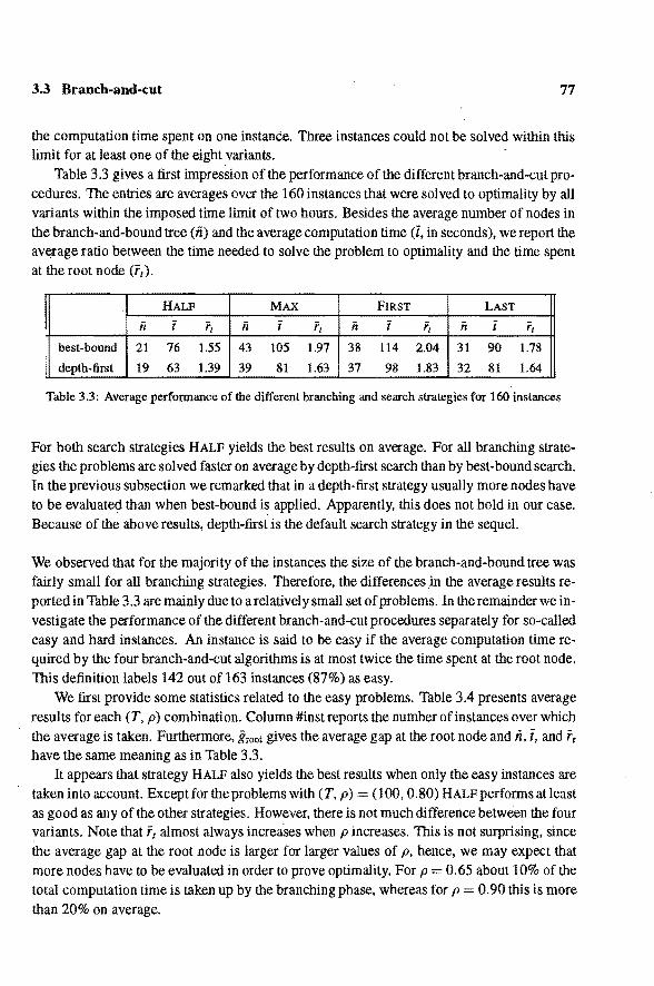
3.3 Brancb-and-cut 77
the computation timespent on one instance. Three instances could not be solved within this limit for at least one of the eight variants.
Table 3.3 gives a first impression of the performance of the different branch-and-cut procedures. The en tri es are averages over the 160 in stances that were sol ved to optimality by all variants within the imposed time limit of two hours. Besides the average number of nodes in the branch-and-bound tree (n) and the averagecomputation time (Î, in seconds), we report the average ratio between the time needed to solve the problem to optimality and the time spent at the root node (f1).
HALF MAX FIRST LAST
ft ï rz ii ï r/ ft ï r/ ft ï ï't
best-bound 21 76 1.55 43 105 1.97 38 114 2.04 31 90 1.78
deptb-first 19 63 1.39 39 81 1.63 37 98 1.83 32 81 1.64
Table 3.3: Average performance of the different brancbing and searcb strategies for 160 instances
For both search strategies HALF yields the best results on average. For all branching strategies the problems are solved faster on average by deptb-fust search than by best-bound search. In the previous subsection we remarked that in a deptb-fust strategy usually morenodes have to be evaluated than when best-bound is applied. Apparently, this does not hold in our case. Because of the above results, deptb-fust is the default search strategy in the sequel.
We observed that for the majority of the instances the size of the branch-and-bound tree was fairly small for all branching strategies. Therefore, the differences in the average results reported in Thble 3.3 are mainly due to a relativel y small set ofproblems. In the remainder we investigate the performance of the different branch-and-cut procedures separately for so-called easy and hard instances. An instanee is said to be easy if the average computation time required by the four branch-and-cut algorithms is at most twice the timespent at the root node. This definition labels 142 out of 163 instances (87%) as easy.
We fust providesome stalistics related to the easy problems. Table 3.4 presentsaverage results for each (T, p) combination. Column #inst reports the number of in stances over which the average is taken. Furthermore, !i root gives the average gap at the root node and ii, i, and fr
have the same meaning as in Table 3.3. It appears that strategy HALF also yields the best results when only the easy instances are
taken into account. Exceptfor theproblems with (T, p) = (100, 0.80) HALFperfarms atleast as good as any of the other strategies. However, there is not much difference between the four variants. Note that f 1 almost always increases when p increases. This is not surprising, since the average gap at the root node is larger for larger values of p, hence, we may expect that morenodes have to be evaluated in order to prove optimality. For p = 0.65 about 10% of the total computation time is taken up by the branching phase, whereas for p = 0.90 this is more than 20% on average.

78 The multi-item DLSP
HALF MAX FIRST LAST
T p #in st i root ii t r, ii ï r, ii t r, ii t r, 0.65 7 0.40 5 9 1.09 5 '9 1.09 7 10 1.13 11 11 1.21
60 0.80 21 0.44 6 16 1.10 8 17 1.13 8 17 1.15 8 17 1.14
0.90 25 0.57 9 24 1.22 15 26 1.31 10 25 1.26 11 25 1.28
0.65 16 0.20 6 29 1.09 8 29 1.11 6 29 1.09 8 29 1.09
100 0.80 31 0.30 16 54 1.24 17 53 1.22 15 55 1.25 11 50 1.15
0.90 42 0.40 12 68 1.21 25 77 1.36 14 71 1.27 19 74 1.33
Table 3.4: Average performance of the different branching strategies for the easy instances
The last table presents results for the 21 hard in stances. For each instanee we give the number of nodes (n) and the computation time (t) required for each of the four different branching strategies. An instanee is identified as I.T.M.D.k, where D denotes the total demand, i.e., D p x T, andk E {1, ... , 27}. Not surprisingly, themajority oftheseinstances bas capacity utilization p = 0.90. Column groot shows the integrality gap at the root node. The timespent before entering the branching phase is reported in column troot· The last row presentsaverage results over the 19 in stances for which no en try '-' appears in the corresponding row. This entry indicates that the problem could not be solved within two hours.
For the 19 in stances for which average results are reported in the last row, strategy HALF yields considerably better results than the other three strategies. No te however that LAST perfarms as least as good as HALF for a fair number of these problems. Moreover, for the two in stances that are not considered in the average results, LAST outperfarms the other strategies by far.
3.4 Related research
In this section we give an outline of two other salution methods for DLSP proposed in the literature. The performance of these methods is compared to the performance of the branchanct-eut algorithm.
Fleischmann [14] proposes a branch-and-bound algorithm using Lagrangeau relaxation for the determination of both the lower and upper bounds. Th is approach is based on the same formulation as our branch-and-cut procedure. Relaxing the coupling constraints I:; x~ :s 1 for all t decomposes the problem into M single-item problems, which are solved by means of dynamic programming (DP). The Lagrangeau multipliers are updated iteratively by a standard subgradient optimization technique. Feasible solutions are obtained by successively solving the subproblems for item i = 1, ... , M by a modification of the DP-algorithm in which the periods already used for the production of item j < i are skipped. The brànching strategy constructs a schedule by fudng the periods one by one in decreasing order. That is, from a

3.4 Related research 79
HALF MAX FIRST LAST
instanee 8tool treo~ n t n. t n t n t
!.60.2.54.13 4.66 27 317 119 533 170 675 295 895 294 1.60.4.54.18 1.50 22 23 41 29 36 21 37 187 153
1.60.4.54.24 1.48 32 31 89 113 137 51 125 25 74
1.60.4.54.25 0.64 33 9 46 105 100 73 129 3 40
1.60.6.48.6 1.49 24 97 116 191 156 189 212 41 78
!.60.6.54.23 1.23 29 35 96 95 130 39 113 29 85
1.100.4.80.24 1.02 84 43 198 449 659 103 418 41 211
1.1 00.4.90.12 0.99 94 115 369 207 439 141 439 295 835
I.1 00.4.90.15 0.65 103 235 803 215 494 245 912 457 1594
1.100.4.90.18 0.64 66 77 211 197 288 499 924 33 101
1.100.4.90.26 1.43 74 119 299 193 317 365 923 39 145
1.1 00.4.90.27 0.94 148 29 286 103 484 75 569 45 360
1.100.6.80.19 1.59 100 335 1630 665 1860 355 1591 737 3865
1.100.6.80.22 0.44 111 17 169 419 825 89 316 31 182
1.1 00.6.90.3 0.71 179 - - - - 559 4186
1.100.6.90.10 1.16 177 665 3083 - - 1631 6540 147 907
1.100.6.90.15 0.48 94 75 277 473 733 697 1253 103 262
1.100.6.90.16 0.53 151 21 227 103 396 389 896 21 208
1.100.6.90.19 1.07 85 33 129 353 671 227 435 1073 1764
1.1 00.6.90.21 0.12 127 231 463 53 211 259 439 5 137
1.1 00.6.90.25 0.26 139 3 156 33 259 159 1001 15 190
Average (19) 1.10 81 97 301 238 440 245 580 214 557
Table 3.5: Performance of !he different branching strategies for the hardinstances
subproblem in which periods t + 1 up to T are fixed, M + 1 new subproblems are created by either assigning production of item i, 1 :5 i :5 M, to period t or leaving t idle.
Cattrysse et al. [7] present a salution metbod for DLSP basedon column generation. This algorithm has been primarily developed for the problem with sequence-independent startup
times. The columns in the master problem represent production schedules for the different items. The metbod is used as a beuristic as it only solves the LP-relaxation of the master problem. The procedure starts with a restricted set of columns and generates new production schedules by solving single-item problems by dynamic programming. These are added to the formulation as long as they price out. A dual aseent procedure foliowed by subgradient
optimization provides approximately optimal dual variables of the LP-relaxation of the master problem. Feasible solutions are obtained from the upper bounding procedure developed

80 The multi-item DLSP
by Fleischmann and from an enumeration algorithm that tries to construct a feasible schedule from the single-item production schedules generaled so far.
Fleischmann tested bis algorithm on data sets from the literature on a capacitated lot-sizing problem with larger time periods during which production can occur for more than one item. This problem is transformed in a discrete lot-sizing and scheduling problem by a discretization of the production periods. Unlike Fleischmann, we can solve most of the probieros TV (T varies between 63 and 96, 8 items, total demand 61) without branching, but his algorithm requires much less computation time. Furthermore, neither ofhis probieros Gl and G2 (250 periods, 3 items, p E {0.84, 0.90})wassolved by our algorithm within onehour. In general, we conclude that the approach based on Lagrangeau relaxation can handle much largerinstances than the branch-and-cut procedure within the same amount of time.
Cattrysse et al. present computational results for a test set of 45 instances with T = 60, ME {2, 4, 6}, and p either :5 0.55, between 0.55 and 0.75, or > 0.75. The cost structure is somewhat different from ours; for more details we refer to [7]. The authors compare the performance of their algorithm to Fleischmann's procedure, where the latter is applied without branching. The column generation approach yields smaller gaps and a larger number of probIeros that are solved to optimality, but requires a larger computational effort. We may expect that, when branching is applied, Fleischmann's algorithm needs less time than the column generation procedure in order to reach gaps of the same size.
Finally, we compare the results reported by Cattrysse et al. to the results that we obtained for our set of 60-period problems. The cutting plane procedure yields slightly better gaps when pis (about) 0.65. For largervalues of p column generation performs better. This also holds with respect to the computation times, although we have no insight into the extra time that will be needed by this approach in order to solve all in stances to optimality. Moreover, we cannot say anything about how the two approaches will compare for largervalues of T.

4. Sequence-independent startup times
In this chapter we study the extension of DLSP in which startups take up an integral number of periods in which no production can occur. We restriet ourselves to the problem with s~uence-independent startup times, i.e., the startup times only depend on the item for which the machine is set up. In Section 4.1 we present an integer programming formulation of the problem that is similar to the formulation ofDLSP studied in the previous chapters. Valid in~ualities for the latter formulation are therefore easily turned into valid inequalities for the problem with startup times. Section 4.2 deals with this subjeetin somemoredetail. InSection 4.3 we discuss a multicommodity flow formulation of the single-item problem. By reformulating the problem as a shortest path problem we derive a complete linear description in the new variables.
4.1 Formulation
The setting for the problem with s~uence-independent startup times, denoted by DLSS, is the same as for DLSP, except that a startup for item i takes up u; periods, u; E z+, in which no production can occur. As before, T denotes the number ofperiods of the planning horizon, M the number of items, and d; E {0, 1} the demand for item i in period t. We assume that the machine is turned off at the beginning of the planning horizon, hence, u; + 1 is the first period in which item i can be produced. As a con~uence, it is always assumed that there is no demand for item i before period u; + 1.
As for DLSP, the binary variablex: indicates whetherproduction occurs for item i in period t or not. If item i is produced in period t, then this incurs a cost c;. Furthermore, we introduce variables z: that equal one if the interval [t u;, t 1] is used for setting up the machine for
item i and zero otherwise. Thus, z: = 1 indicates that a production batch of item i can be started in period t. Associated with z: is the startup cost g;. Obviously, x: and z; are only defined for t E [a;+ 1, T].
If startups do not affect the production capacity, then there exists a production schedule that satisfies all demand in time if and only if Li dL, s t for all t (cf. Section 3.1 ). In the presence of startup times, however, the existence of such a production schedule is not easily established. In order to prevent infeasibility of an in stance, we therefore assume that the demand can always he satisfied by producing out of the regular production periods. This incurs a penalty cost c~ per unit of item i. The nonnegative integer variabie X~ represents the total number of units of item i produced in this way. For convenience, this production is said to occur in period 0. In practice, XJ may correspond to the demandquantity of item i that cannot he satisfied, in which case eb X& represents the lost purchases.
Now DLSS can he formulated in the following way:
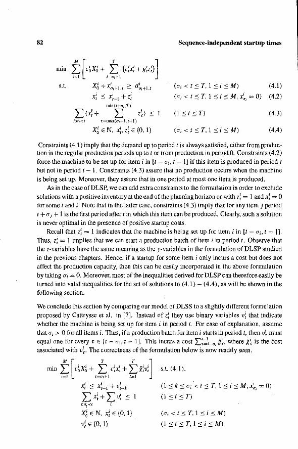
82 Sequence-independent startop times
s.t. XJ +x~,+I.t ;:: d~<+1,t xi < xi +z' t - t-1 I
min (t+u;, T)
:L<x:+ L z~) < 1 i:u1<t -c=max(u;+1.t+l}
X~ EN, X~, z: E (0, 1}
(a; < t s T, 1 sis M) (4.1)
(a, < t s T, 1 sis M, X~1 0) (4.2)
(1 st sT) (4.3)
(a; < t s T, 1 si s M) (4.4)
Constraints ( 4.1) imply that the demand up to period t is always satisfied, either fromproduction in the regular production periods up tot or from production in period 0. Constraints (4.2) force the machine to be set up for item i in [t -a;, t- 1] if this item is produced in period t but not in period t - 1. Constraints ( 4.3) assure that no production occurs when the machine is being set up. Moreover, they assure that in one period at most one item is produced.
As in the caseofDLSP, we can addextraconstraints to the formulation in order to exclude solutions with a positive inventory at the end of !he planning horizon or with d = 1 and x~ = 0 forsome i and t. Note that in the latter case, constraints (4.3) imply that for any item j period t +a j + 1 is the first period after tin which this item can be produced. Clearly, such a solution is never optima! in the presence ofpositive startup costs.
Reeall that z: = 1 indicates that the machine is being set up for item i in [t- a;, t- 1]. Thus, z! = 1 implies that we can start a production batch of item i in period t. Observe that the z-variables have the same meaning as the y-variables in the formulation of DLSP studied in the previous chapters. Hence, if a startup for some item i only incurs a cost but does not affect the production capacity, then this can be easily incorporated in the above formulation by taking a; = 0. Moreover, most of the inequalities derived for DLSP can therefore easily be turned into valid inequalities for the set of solutions to ( 4.1) - ( 4.4 ), as will be shown in the following section.
We conclude this section by camparing our model ofDLSS toa slightly different formulation proposed by Cattrysse et al. in [7]. Instead of z: they use binary variables v: that indicate whether the machine is being set up for item i in period t. For ease of explanation, assume tb at a; > 0 for all items i. Thus, if a production batch for item i starts in period t, then v~ must equal one for every r E [t - a;, t 1]. This incurs a cost 1:~~11_.,., g~. where g~ is the tost associated with v~. The correctnessof the tormulation below is now readily seen.
min t [c~X~ + 1
t.1 c~; + tg~v;]
x! s x~_ 1 + v~-k :Lx~+ I>: s i:u!<t i
X~ E N, x: E {0, 1}
V~ E {0, 1}
s.t. (4.1),
(1 s k sa;< t sT, 1 sis M, x~, = 0)
(1 st sT)
(a; < t s T, 1 sis M)
(1 s t s T, 1 s i s M)
4.2 Valid inequalities 83
Observe that fora; > 1 there exist solutions (X0 , x, v) with v; = 1 for k subsequent periods, where kis not a multiple of a;. Such a solution does not correspond to any feasible solution
to (4.1)- (4.4). However, one easily verifies that if (X0 , x, z) satisfies (4.1)- (4.4), then
(Xo, x, v) with min(Hu;, T)
v~ L z~ ~=max(u;+I.HI)
for all i and t is a solution to the above formulation. In particular, if g; = L~~11_"., g~ and g; > 0 for all i and t, then both formulations yield the same optimal solution to DLSS. Furthermore,
it is not difficult to show that if g; = L~~~-u, g~ for all i and t, then the LP-relaxation of our model yields lower bounds that are as least as good as the lower bounds obtained from the
LP-relaxation of the model proposed in [7].
4.2 Valid inequalities
In this section we give some results on valid inequalities for DLSS. We mainly con si der valid
inequalities for the single-item problem, i.e., inequalities that are valid for all (Xo, x, z) satisfying
Xo+Xu+l,t ~ du+l,t (a < t:::; T) (4.5)
Xt ::S Xt-1 + Zt (a < t:::; T, x".= 0) (4.6) min(t+u,T)
Xt+ L Zt :::; 1 (a :::; t :::; T, x". = 0) (4.7) ~=t+l
Xo EN, Xr, Zt E {0, 1} (a<t::ST) (4.8)
where T denotes the number ofperiods and dr E {0, 1} for all t <d1,u = 0). For ease ofpresentation, we renumber the periods such that period 1 is the first period in which production can
occur. Let T denote the last period of the new planning horizon, i,e., T = t - a. Moreover,
define d 1 = dt+"., 1 :::; t :::; T. Then the above formulation can be restated as
Xo + x1.r ~ di.t (l:::;t:::;T) (4.9)
Xr ::S Xt-1 + Zt (1 S t ::S T, Xo = 0) (4.10) min(t+u,T)
Xt+ L z~ :::; 1 (0 ::S t ::S T, Xo = 0) (4.11) ~=t+l
Xo EN, Xr, Zt E {0, 1} (1 :::; t:::; T) (4.12)
Let X,. denote the set of feasible solutions to (4.9)- (4.12). Every valid inequality for X,.
clearly yields a valid inequality for thesetof feasible solutions to (4.5) - (4.8) by substituting
x1+". and Zt+u for x1 and Zr. respectively, for every tE [1, T].
Let a > 0. Because of (4.11), we have X, c x,._1 and conv(X,) c conv(X,_ 1). Thus,
all valid inequalities for x,._1 are valid for X,. In particular, all valid inequalities for -Xó are

84 Sequence-independent startop times
valid for .X:,.. Obviously, the subset of solutions in ;\ó with Xo = 0 is the set of solutions to the formulation of the single~item DLSP studied in Chapter 2 with y1 replaced by z1• For the latter fotmulation we derived several classes of facet-defining inequalities ax + {Jz ~ y with a1 E {0, 1} for all t. Reeall that these inequalities can be written as Ir ~ LB(x, z), i.e., they yield alower bound on theinventory Ir at the end ofperiod t. Ifproduction mayalso occur in period 0, then Ir= Xo + Xt,r- dt,r· Thus, the inequalities from Chapter 2 become valid for ;\ó by actding the term Xo to the left-hand side. It is nothard toseethese inequalities are also facet-defining for conv(;\ó).
For two subclasses we will give conditions for the inequalities to be facet~defining for conv(.X:,.). However, we will notprove in detail that an inequality defines a facet since these proofs are simHar to the proofs in Chapter 2. As a matter of fact, they are usually facilitated by the possibility to produce in period 0. The following lemma implies that, in order to prove that an inequality defines a facet of conv(.X:,.), one has to construct 2T linearly independent direcUons in the subset of solutions in .X:,. that satisfy the inequality at equality.
Lenuna 4.2.1 Conv(.X:,.) has dimension 2T + 1 for all u ~ 0. D
Since demand can always be produced in period 0, one readily constructs the 2T + 1 unit vee~ tors as directlans in .X:,.. It is obvious that there always exists a feasible salution with Xo 0 for the single-item DLSS. However, if the variabie Xo is omitted from the formulation, then thedimension oftheconvexhull of .X:,. depends on thedemand function. Forexample, if u= 2 and d2 = 1, then all solutions in Xz with Xo 0 satisfy x1 + zz 0 and Z3 = 0.
The following lemma gives a necessary condition for an inequality to be facet-defining for conv(.X:,.).
Lenuna 4.2.2 Let u> 0. Let aoXo + ax+ {Jz ~ y be afacet-defining inequality ofconv(.X:,.) that is not oftheform (4.11 ). Thenfor any t :S T- u thefollowing holds:
Cl. There exists a salution in .X:,. without production in the interval [t, t +u] that satisfies the inequality at equality.
PROOF. Define .,t. = { (Xo, x, z) E .X:,. : aoXo +a x+ {Jz = y}. From the assumption that a x+ {Jy ~ y de fin es a facet of conv(.X:,.) and is not of the form ( 4.11), it follows that for any t :s T u there mustbeat least one solution ( Xo, x, z) E ..t. satisfying Xr + Zt+l .t+cr = 0. Since x1 + Zt+l,t+cr = 0 implies that no production occurs in [t, t +u], this proves the statement. D
We discussed before how facet-defining inequalities derived in Chapter 2 cari easily be turned into valid inequalities of .X:,.. In the sequel, we will give conditions for the inequalities of two subclasses to be facet~defining of conv(X,.). For all inequalities Xo + ax + {Jz ~ yin these subclasses the following holds: for any t E [1, T -u] there exists a salution in X- satisfying X0 + ax + {Jz = y + 1 and Xr + Zr+t,t+cr = 0. The following lemma showshow such an in~ equality can be strengthened with respect to conv(X,.) when condition Cl is violated forsome period t.

4.2 Valid inequalities 85
Lemma 4.2.3 Let a> 0 and tE [1, T-a]. Let Xo + ax + f.lz;::: y be as described above.lf there is no solution in X:,. without production in [t, t +a] that satisjies the inequalityat equality, then
Xo + ax + f.lz + Xt + Zt+l,t+tr ;::: y + 1 (4.13)
is validfor x;,. anddejines a higher-dimensionaljace jorconv(X:,.) than the original inequality. 0
lt is nothard to see that if Cl is also violated fort and a' < a, then (4.13) is valid for .:V as well. However, the new inequality does not necessarily define a higher-dimensional face with respect to conv(..:V).
Example 4.2.1 Let T 6 and ds = d6 = 1. Then
+ Z5 > l Xo + X1 + Xz + X3 + X4 -
defines a facet of conv(.:\á) but not for conv(Xi ), since for any solution in .M and, hence, in Xi that satisfies the inequality at equality production occurs in at least one of the periods 5 and 6 (see also Proposition 4.2.4 below). By Lemma 4.2.3
+ Z5 + Z6 ::: 2
is valid for .M and X1• Moreover, the inequality defines a facet ofboth conv(XJ) and conv(Xi). 0
We fust consider theLSM inequalities (cf. Subsection 2.2.4), which have the following form:
Xo+Xt,t+ L(Xt+j+Zt+j+l,sdq,1);::: d~,t+lll. jE]
(4.14)
where t E [0, T- 1], dt+1 0, J 5:; {1, ... , dt+J,T}, and where Sd(t,J) denotes the jth demand period after t. These inequalities are facet-defining for conv(.:\á).
Proposition 4.2.4 Let a> 0. lnequality (4.14) de.fines a facet ojconv(X:,.) if and only iffor every j E {1, ... , dt+J,T} the following holds: if Sd(t, J) :::;: t + j +a, then j E J. 0
The necessity of the condition follows from the observation that for jE {1, ... , dt+t,r}\1 there is no solution in .:\á, and, hence, none in x;,., without production in [t + j, Sd(t,Jl] that sat
isfies (4.14) at equality. By Lemma4.2.3, we can add Xt+j + Zt+j+l •. rd<r.J) ;::: 1 to (4.14). This obviously yields another inequality of the form (4.14) with J' = JU {j}.
86 Sequence-independent startup times
We next consicter the RSM inequalities (cf. Subsection 2.2.2), which can be written in the form
Xo+Xt,e•+ L(Zu+l,u+d.,,. -Xu+d.,,.) ~ dt,e•, u EU
(4.15)
where t* is a demand period and U s; {t: t < t* and de= 0}. For convenience, define V= {u +du,t• :u E U}. Moreover, denote by u(v), v E V, theelementin U satisfying u+ du,t• v. Again, these inequalities are facet-defining for conv(~).
Unlike in the case of constraints (4.14), we can only give sufficient conditions for (4.15) to be facet-defining for conv(X,.), a> 0. We use the following notation with respect to an inequality of the form ( 4.15): if t* is not the last demand period, then t' denotes the fust demand period after t*, otherwise we set t' T + 1. Furthermore, define Vmin = minvEV v.
Proposition 4.2.5 Let a > 0. Ij t' > min ( T, t* + a+ 1) or if t' = t* + a + 1 and (V min + a S t* ort* E V), then inequality (4.15) defines a facet ojconv(X,.) D
With respect to conv(Xt) we can give both necessary and sufficient conditions for (4.15) to define a facet. These are easily obtained from the following lemma, which provides astrong relation between facet-defining inequalities of conv(~) and conv(Xi).
Lenuna 4.2.6 Afacet-defining inequality ojconv(~) defines a facet of conv(Xt) if and only ij for every t < T there exists a solution in Xi without production in [t, t + l] that satisfies the inequality at equality.
PROOF. We already proved the necessity ofthe condition. Hence, let aoXo + ax + {Jz ~ y be a facet-defininginequality ofconv(~). and denote by Xr theset ofsolutions in X,., a E {0, 1}, that satisfy the inequality at equality. Moreover, suppose that for every t < T there exists asolution in% without production in [t, t + 1]. Since the inequality defines a facet of conv(~). there exist 2T linearly independent directionsin ,Xö (cf. Lemma 4.2.1). The direction e(z1)
is easily established for all t > 1 with fJr = 0, where e(z1) denotes the unit vector of length 2T + 1 corresponding to the variabie ze. We may assume that the other directions are obtained from solutions in% that satisfy Xt + Zt+ 1 S 1 for all t, thus, these are directionsin Xi as well. Hence, it suffices to show that e(ze) is also a direction in% for all t > 1 with fJr = 0. To that end, let t > 1 satisfy fJr 0. By assumption, there exists a solution (Xo, x, z) E Xi sat-
isfying Xt-1 +Ze = 0. Then (Xo, X, z) with Ze 1 and zt' z.- for r i= t is also in Xi and (Xo, X, Z) (Xo, X, Z) e(Zt). D
It is not likely that a simpte relation between the facet-defining inequalities of conv(X,.-1) and conv(X,.) can be established fora > 1. In any case, the following example shows that the above result fora 1 does not hold for general a.

4.2 Valid inequalities 87
Example 4.2.2 Let T = 10 and d1 = 1 fortE {7, 8, 9, 10}. Then
+ Z3 + 2z4 + Zs + Z7 + Zs
Xo + Xt + X2 + X3 + X6 + X7 ~ 2 (4.16)
is an inequality öfthe form (4.15) with t* = 8 and U= {2, 3, 6} that defines a facet of conv(X1)
(cf. Proposition 4.2.7 below). Furthermore, for each tE [1, 8] there exists a salution in X2 without production in [t, t + 2] that satisfies (4.16) at equality: take Xo = 2, z9 = x9 = Xto = 1 fort :::; 6, and X0 = 0, z2 = x2 = ... = xs = 1 fort= 7, 8. However, (4.16) does not define a facet of conv(X2), since x1 + zs = xs for all (Xo, x, z) E Xz that satisfy the inequality at equality. 0
Let us consicter inequalities (4.15) again. Throughout, we use the following notation with respect to such an inequality: Î = max{t E [t*, T] : dr: = 1 for all TE [t*, t]}. For every inequality of the form (4.15) condition Cl is satisfied with respect to X1 fort < t* and fort ~ î, i.e., forthese periods t there exists a salution in X1 without production in [t, t + 1] that satisfies (4.15) at equality. Fort E [t*, î- 1] the condition is satisfied if and only if one of the following holds: (i) Î = t*, (ii) Î = t* + 1 and Vmin < t*, or (iii) Î > t* + 1 and { v, v + 1} s; V for some v < t*. Hence, by Lemma 4.2.6, we have the following result.
Proposition 4.2. 7 Inequality ( 4.15) defmes a facet of conv(Xt) if and only if one of the fol
lowing holds: (i) î = t*, (ii) Î = t* + 1 and Vmin < t*, ar (iii) Î > t* + 1 and {v, v + 1} s; V for
some v < t*. 0
The above result implies that ( 4.15) does not define a facet of conv(Xi) if either î ~ t* + 1 and Vmin = t* or î ~ t* + 2, V min < t*, and v + 1 f/. V for any v E V. Denote by R the set of periods t that vialate condition Cl with respect to Xi. Then R = [t*, î- 1] if î ~ t* + 1 and Vmin = t*,
and R = [t* + 1, î- 1] otherwise. Inequality (4.15) can now be strengthened with respect to conv(X1) by applying Lemma 4.2.3 for at least one tE R. The question is: for which R' s; R is
Xo + Xt,t• + L(Zu+l,u+d..,,.- Xu+d..,,.) + L(Xr: + Zr:+l) ~ dt,t• + IR'I (4.17) uEU r:ER'
facet-defining for conv(Xt)? First, notice that if V min = t*, then ( 4.15) is also of the form ( 4.14) with t = u(t*) - 1 and
J = {1, ... , t*- u(t*) + 1}. Then, by Proposition 4.2.4, (4.17) defines a facet of conv(X1) if and only if R' = R = [t*, î- 1]. lt is also not difficult to check that if î ~ t* + 2, 1 VI = { v}, and v < t*, then ( 4.17) defines a facet of conv(XJ) if and only if R' = R = [t* + 1, î- l]. For the remaining cases we have the following result:
Proposition 4.2.8 Let ( 4.17) satisfy î ~ t* + 2, IV I ~ 2, and v + 1 f/. V for any v E V. Fur
thermore, let R' = {t* + 2j -1: j = 1, ... , L(Î- t*)/2J}. Then (4.17) is validfor X1• The
inequality defmes a facet ojconv(XJ) if and only ifone ofthefollowing holds: (i) î = t* + 2,

88 Sequence-independent startop times
(ii) there exists v E V such that v + 2 E V or u(v) exists v E V such that v + 3 E V or u ( v) = v - 2.
v 1, or (iii) î- t* is even and there
0
In all cases, the validity of (4.17) for X1 can be shown by sequentially applying Lemma 4.2.3 to the elements of R' in increasing order. Obviously, if (Xo, x, z) E Xl \X1, then the solution obtained from (Xo, x, z) by setting Zt to zero for all t satisfying Xt-1 = Zt = 1 yields a solution in X1. Hence, a valid inequality for X1 with nonnegative z-coefficients is also valid for XJ. In particular, ( 4 .17) is valid for Xl if it is valid for Xi. Moreover, it is not difficult to show that (4.17) defines a facet of conv(XJ) whenever the inequality is valid for XJ. Then, by Lemma 4.2.6, the result that (4.17) defines a facet of conv(X1) for the given set R' is establîshed by checking that for any t E R there exîsts a solution in Xi without production in [t, t + 1] that satisfies ( 4.17) at equality.
Example 4.2.3 Let T = 10 and d1 1 fortE [5, 10]. Then
+ Z3 + Z4 + Z5 + Z6
Xo + x1 + x2 + X3 + Xs
defines a facet of conv(XJ) but not for conv(X1), since Xz-l + Zt = 1, tE [8, 10], for any solution (X0 , x, z) E X1 that satisfies the inequality at equality. Now the above proposition yields that
+ Z3 + Z4 + Z5 + Z6 + Zs + Zto > 4 +x9 -Xo + X1 + X2 + X3 + X5
defines a facet ofboth conv(XJ) and conv(Xt). Notice that this inequality does not belong to any of the three subclasses of facet-defining inequalities of conv(XJ) that were discussed in Subsectiens 2.2.2 through 2.2.4. 0
Let us finally show how the multi-item inequalities (3.12) (cf. Sectîon 3.2) can be strengthened in the presence of startup times. Consicter the multi-item formulation presentedat the beginning of this chapter. For convenience, we add x~ = z; = 0 for all i and t ::::; a;. Then the following modification of (3.12) is valid for the set ofsolutions to (4.1)- (4.4):
t,
X~ + xL,-1 2:: dL,-1 + d!,,1, :L)x/2 - z{t+Lr) - L d:,1,z;, (4.18) jEJ t=tz+l
where i E {1, ... , M}, J ç {1, ... , M} \{i}, and t 1, t2, and t3 are three periods that satisfy 1 ::::; t 1 ::::; t2 ::::; t3 ::::; Tand dL, 2:: 1. These inequalities werederived from thé following observation: if there is no production for item i in the interval [lt, t'], where t' E (t2 + 1, t3], then the inventory for item i at the end of period t1 - 1 must beat least d1 r. If startup times are
" zero, then there is no production for item i in [t1, t2] if the whole interval is used for produc-tion of item j. The latter is implied by x{, - zf +I 1 1. In the presence of positivè startup
"' 1 , 2
times, however, we cannot produce item i in the interval [t1, tz] if all periods in [t1 + a j, tz]
are used for production of item j, which is implied by x/2
- z~+o)+1 . 12 = 1. Moreover, if item
4.3 A multicommodity ftow formulation 89
j is produced in period t2, then t2 +a; + 1 is the first period after t2 in which production for item i can occur. The above inequality can therefore be strengthened to
x~ + xL~-1 2: dL~-1 + d:t.ll L:<xf,- zfi+l7j+1.r)- t d;,t,z;. <4.19) jEJ t=t2+a;+1
Reeall that inequalities (4.14), (4.15), and (4.18) (with X~= 0 for all i) servedas cutting plan es in the branch-and-cut algorithm for DLSP discussed in the preceding chapter. Obviously, the separation routinescan be used in a cutting plane algorithm for DLSS as well. The strengthenings of inequalities ( 4.1 5) or ( 4 .18) presented above can easily be incorporated. Computational experiments will have to show whether the actdition of these inequalities is as effective in reducing the integrality gap for DLSS as for DLSP.
4.3 A multicommodity flow formulation
A natura! formulation for single-item lot-sizing problems is the one in which the variables are only indexed by t. However, the introduetion of new variables often yields a tighter formulation with fewer constraints. Various types of extended formulations are discussed in the literature; fora review we refer to Pochet and Wolsey [33]. In many cases a complete linear description in the new variables is derived.
One such extended formulation is the multicommodity flow formulation, in which the production variables x, are split into variables X1k that specify how much is produced in period t to satisfy the demand in the kth demand period. Van Hoesel and Kolen [20] present a multicommodity flow formulation for DLSP in which not only the production variables x, but also the startup variables y, are split. By rnadeling DLSP as a shortest path problem they derive an LP-formulation in these variables that always yields an integral solution.
Here we give a similar result for the single-item problem with startup times. We consicter DLSS with the additional restrictions that we always produce when the machine has been set up for production (z1 :::; x1) and that overproduction is not allowed. As in Section 4.2, the periods are numbered such that period 1 is the first period in which production can occur. Thus, we consicter the following formulation of DLSS:
T min coXo + L (CrXr + g,Zr)
1=1 s.t. Xo + Xl,t 2: d1,t Ost<T) (4.20)
Xo+X1,T d1,T (4.21)
z, S Xz S Xz-1 +zz (1 s t s T, Xo = 0) (4.22) rnin(t+17,T)
x,+ I: Zr S 1 (0 st sT, Xo 0) (4.23) l=t+l
Xo EN, Xz, Zt E {0, 1} (1 st sT) (4.24)

90 Sequence-independent startup times
In a multicommodity ftow formulation of DLSS the variables x1 and Zr are split into binary variables Xrk and Ztk• respectively. As usual, Sk denotes the kth demand period. Then Xrk = I if and only ifproduction occurs in period t to satisfythe demand in sk. Similarly, Zrk = I if and only ifperiod t is used to produce forperiod Sk aftera startup in [t- (1, t- 1]. The integer variabie X0 is split into binary variables Xok that indicate whether the demand for period sk is produced in period 0. Withoutlossof generality we assume that the demand forSt. k > I, is not produced before the demand for Sk-I, i.e., we only consider solutions to DLSS that satisfy
if Xr1,k-I = Xr2,k = I, then ti < tz or ti = tz 0. (4.25)
In the sequel a complete linear description of the convex huil of the set of these solutions will be established. The result is obtained by modeling DLSS as a shortest path problem on an
acyclic network such that the variables Xrk and Zrk form a subset of the ftow variables in the conesponding linear program. Elimination of the other variables yields a linear program in the x- and z-variables that always bas an optimal integral solution.
We fust present a dynamic programming algorithm that solves DLSS. This algorithm will be transformed into the shortest path formulation mentioned above. For convenience, define
K {I, ... ,d~,r}. Now let tjJ(t, k), t E [1, sk] and k E K, denote the minimumcostof a solution for periods
0 up to t in which period t is used for production and the total production up to t equals k. If t < k, then the production in period 0 is at least k-t, which incurs a cost of c0 per unit. Also observe that if t E [2, C1] is used for production and the total production up to t equals k > 1, then either t is the first period in [1, t] in which production occurs or period t - 1 used for production as well.
Furthermore, let lfr(t, k), t E [2, Sk- C1] and k E K, denote the minimumcostof a solution for periods 0 up tot for which the following holds: period t is not used for production, period
t I is not used for setting up the machine, and the total production up to t equals k 1. In this case the kthunit cannot be produced before t + (1. Hence, lfr(t, k) is only defined for
t 'S. sk (1, Note that if the (k- 1 )st unit is produced insome period t E [sk- (1 + I, sk-I + 1 ], then the kth unit must be produced in period t + I. Moreover, if the kth unit is produced in t > Sk-I+ 1, then a startup occurs in the interval [t (1, t- 1].
Using the above observations we obtain the following forward recursion is easily verified:
tjJ(t, I)
t/J(t, k) =
Cr+
gr+Cr fortE [1, sJ], and
co(k -1)+ gl min(co(k -1) + g1, t/J(t -1, k-1)) min(tjJ(t- 1, k 1 ), lfr(t- C1, k) + gr)
lfr(t (1, k} + gt
tjJ(t -1, k 1}
fort= 1 fortE [2, (1 + 1] fortE [C1 + 2, min(sk-1 + 1, sk- C1)]
fort E [Sk-I + 2, sk-a]
fortE [Sk- C1 + 1, Sk-I+ 1]

4.3 A multicommodity flow formulation
'1/f(t, k) = {
min(co(k-l),<P(l,k 1)) min('!fr(t -1, k), <P(t -1, k -1))
t(t- 1, k)
fort= 2 fortE [3, min(Sk-1 + 1, Sk-a)]
fort E [Sk-I + 2, Sk a]
91
for k E K\{1}. Çalculation of min (codi,T, minre[l,s•1.rJ <P(t, dt,T)) yields the minimum cost
of any feasible solution to DLSS.
The dynamic programming algorithm gives rise toa shortest path tormulation in the following way. For convenience, define Kt = K\{1}. Wedefine a network that, apart from a soureeS and a sink S', consists of the following nodes:
• Urk for all tE [0, Sk] and kEK, except for (t, k) = (0, dt,T);
• Vrk for all tE [2, Sk-I+ 1] and k E Kt;
• Wrk for all tE [2, Sk-a] and k E Kt.
Every solution to DLSS will correspond toa path from S to S'. Node Urk will be on the path if and only ifthe kthunit of demand is produced in period t. Node Vrk will be on the path if and only if the demand for Sk-1 is produced in period t- 1. Finally, node Wrk will be on the path if the following holds: there is no production in period t, the total production up to period t equals k 1, and the machine is not being set up in t - 1.
Table 4.1 lists the arcs in the network together with the corresponding flow variabie and cost. Figure 4.1 shows the network corresponding to the instanee with T = 6, a 2, and demand periods s1 = 2, s2 = 5, and S3 6.
are variabie fined for
(S, Uot) Xot co
(S, u,1) Ztt g, tE[l,sJ]
(uo,k-1, uok) XQk co k E Kt \{dt,T}
(uo,k-1, u,k) Ztk g, tE[l,a+l]andkEKt
(uo,k-1, W21<) Ytk 0 kEKt
(Ur-l,k-1, Vrk) Xr-t,k-1 Cr-I tE [2, sk-I + 1] and k E Kt
( v,k, Urk) fttk 0 tE [2, sk-I + l] and k E Kt
(Vtk> Wrk) fJ,k 0 tE [2,min(sk-t +l,sk a)] and k E Kt
(wrk• w,+t,k) Ytk 0 t E [2, sk - a- 1] and k E K1
( Wtk, Ut+.,.,k) Zt+.,.,k 8t+D' t E [2, sk - a] and k E Kt
(uo,dt.r-t. S') XO,dt,T co
(ur,d1 T'S') Xt,dtT c, tE[1,sd1 rl
Table 4.1: Arcs in the network
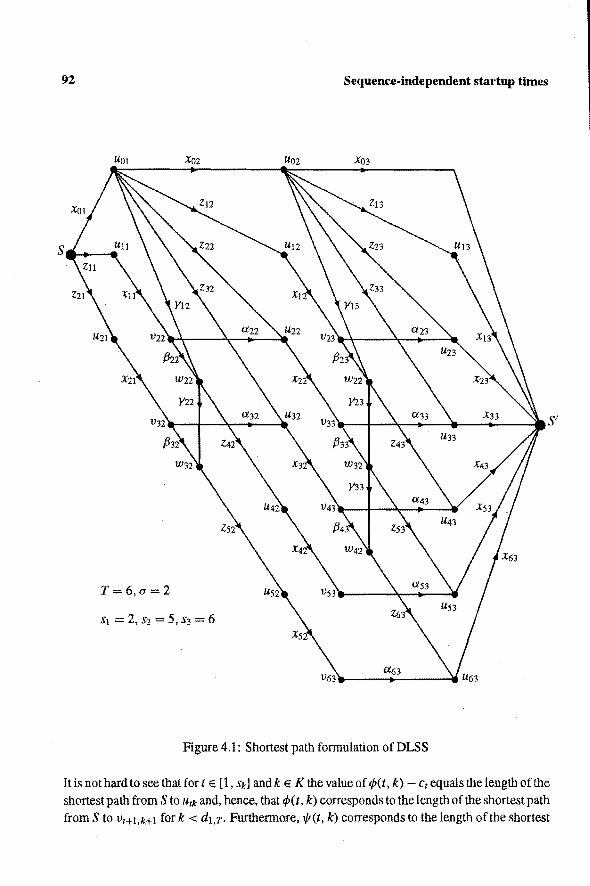
92 Sequence-independent startup times
uo1 Xoz Uoz Xo3
T= 6, a= 2
St = 2, Sz = 5, S3 = 6
Figure4.1: Shortest path formulation ofDLSS
lt is nothard to see that fort E [1, Sk] and k E K the value of rp(t, k) - Cr equals the lengthof the shortest path from S to Urk and, hence, that rp(t, k) corresponds to the length ofthe shortest path
from S to Vr+l,k+l for k < dl.T· Furthennore, 1/t(t, k) corresponds to the length ofthe shortest

4.3 A multicommodity flow formulation 93
path from S to Wz~c. Note that the unique shortest path from S to uo~c. k < d1,T• has length cok. Thus, the lengthof the shortest path from S to S' is min(codJ,r. minzE[t,sd
1,rJ q)(t, dt,r) ).
Hence, DLSS can be solved by solving the shortest path problem on this network. Consicter a path from S to S'. Observe that the intermediale nodes are nondecreasing in
both the index t and the index k. Thus, for every k < d 1,r there is precisely one node u1~c, t E [0, s~c], on the path, hence, X11c = 1 for precisely one t E [0, s~c]. The latter also holds for k = dt,T· Furthermore, if Xok 1, k > 1, then Xo,k-t = 1, and if Xtk = 1 fort> 0 and k > 1, then x'!',k-t = 1 forsome r < t. Thus, (4.25) is satisfied. Note further that Ztl< = 1 implies Xrk 1. Finally, if Z11c 1 for k > 1, then X-r,k-t = 1 forsome r ::;: max(O, t a 1 ).
The other variables can be interpreled as follows. If ark = 1, then the demand for Sk-t is produced int 1 and the demand fors" is produced in period t. If flrk 1, then the demand for sk-I is produced in t - 1 but there is no production in period t. Finally, if Ytk = 1, then there is no production in period t and the total production up to t equals k - 1. Moreover, period t is not used for setting up the machine.
The shortest path problem can be solved by the linear program formed by the flow conservation constraints and the nonnegativity constraints. The flow conservalion constraints yield explicit expressions for the a-, {1-, and y-variables in terms of the x- and z-variables. Using these and the nonnegativîty constraints, we can obtain an equivalent linear program in the xand z-variables only. It is a tedious but straightforward procedure to check that eliminabon of the a-, {1-, and y-variables yields the linear program
St
s.t.l:xlk = 1 1=0
Zti = Xtt
Ztk = Xtk
for kEK
for t E [1, st]
fortE {1} U [s~r.-I + 2, s~c] and k E Kt
(4.26)
(4.27)
(4.28)
(4.29)
Ztk ::;: Xtk ::;: Xt-I,k-l + Ztk
Ztk ::;: Xrk = Xt-l.k-t + Ztk
fortE [2, min(s~r.- a, s~c-t + 1)] and k E Kt (4.30)
fortE [sk-a+ 1, s~r.-t + 1] and k E Kt (4.31) st-! t+u
l:x>',k-1+ L Z-rk < 1'=1 1'=1+1
Xok. X1k, Z1k 2: 0
Sk L X'!'k fortE [1, Sk a 1] and k E Kt '!'=t+t
fort E [1, Sk] and k E K
(4.32)
(4.33)
From the above discussion it follows that the linearprogram (4.26) (4.33) always yields an integral solution. Hence, we have proven the following result:
Theorem 4.3.1 The linear program (4.26)- (4.33) solves DLSS. D
A fonnulation for the multi-item DLSS in the variables x;k and z;" is obtained by taking the

94 Sequence-independent startup times
single-item formulations for the different items together with the linking constraints
(4.34)
Obviously, its LP-relaxation will not yield an integral solution in general. However, it is expected to give stronger lower bounds than the LP-relaxation of the formulation in the natural variables. A disadvantage of the multicommodity flow formulation is its large number of variables, which is about d1.r T. If the formulation is used in a branch-and-cut algorîthm, then it may be computationally advantageous tostart with an LP-formulation in which only a subset of the variables is included and to add nonactive variables only when they price out. This is an interesting topic for further research.
5. The delivery man problem
This chapter deals with the delivery man problem or DMP for short. This problem is a variant of the well-known traveling salesman problem (TSP) in which the objective is to find a tourstarting from a given depot that minimizes the sum of the waiting times of the customers. The DMP can also be interpreled as a single-machine scheduling problem with sequencedependent processing times in which the total flow time of the jobs bas to be minimized.
Polyhedral methods have been proven to be very successful for the TSP and many of its extensions. Most of these extensions deal with extra conditions on the graph structure, e.g. preeedenee constraints, such that the problem can still be formulated as a 0 - 1 model. However, we will formulate the DMP as a mixed integer programming problem by introducing time variables (Section 5.1). This formulation can easily be adapted to the problem with time windows, i.e., when each customer bas to be visited within a specified interval. Only a few papers deal with this kind of extension. Ascheuer [2] bas developed a branch-and-cut code for the TSP with time windows. Escudero and Sciomachen [12] and Escudero, Guignard, and Malik [13] study the sequentia! ordering problem with time windows, where the sequential ordering problem is the problem of finding a minimum weight Hamiltonian path subject to preeedenee constraints. For this problem Maffioli and Sciomachen [26] propose a formulation that is similar to our formulation of the DMP.
In Section 5.2 we will derive additional classes of valid inequalities in order to strengthen the linear programming relaxation. The quality of the lower bounds obtained from the LPrelaxation and the effeetiveness of the new inequalities in reducing the gap are studied computationally inSection 5.3.
This chapter ditiers from the previous chapters in that it is primarily devoted to the DMP instead of the DLSP. Nevertheless, the formulation presenled bere may also serve as a basis for a polyhedral approach to the DLSP with sequence-dependent startup times. To that end, we use the reformulation of the latter problem as a TSP with time windows (cf. Seetion 1.2). The DLSP then only differs from the DMP with time windows as far as the objective function is concerned.
5.1 Formulation
The delivery man problem is formally stated as follows. We consicter the complete directed graph G = (V U {0}, A}, where V= {1, ... , n}. With each are (i, j) we associate a nonnegalive integer travel time Pi i· It is assumed that visiting time is included in the travel time, hence, the arrival time at node i equals the departure time at node i. Node 0 is the depot, i.e., every tour starts and finishes in node 0. Furthermore, we assume that every tour starts at time 0.

96 The delivery man problem
Then the waiting time of the customer located at node i is equal to the departure time at node i. Now the problem is to find a tour that minimizes the sum of the departure times at the nodes.
The DMP can be modeled using the following two types of variables. For every are (i, j) there is a binary variabie X; i that indicates whether the are (i, j) is included in the tour or not, and a time variabie t;i defined as follows:
{ departure time at node i, 0,
if Xij 1, otherwise.
Since we assume that every tour starts at time 0, the variables toj can be omitted from the model. This gives rise to the following formulation of DMP, in which C denotes a large con-stant:
n n
min L L: t;j
i=l j=O.j#i
" s.t. L: Xij 1 (0 5. i 5. n) (5.1)
j=O,j#i
n
L: Xij = 1 (0 5. j 5. n) (5.2) i=O,i#j
n n n
L: t;j + L: PijXij L: t jlc (1 5. j 5. n) (5.3) i=l.i#j i=O,i,fj k=O,k,fj
0 5. t;j 5. CXij (0 5. i, j 5. n, i =1= j, i =1= 0). (5.4)
X;j E (0, 1} (0 5. i, j 5. n, i =1= j) (5.5)
Constraints (5.1) and (5.2) ensure that every node, including thedepot, is visited exactly once. Constraints (5.3) guarantee that if Xij 1, then the departure time at node j equals the departure time at node i plus the travel time Pii· These constraints also prevent subtours, unless there exists a set of subtours such that every node is in precisely one subtour and Pii = 0 for all arcs {i, j) that are involved in these subtours. If Cis an upper bound on the departure time at node i, e.g. C = n · max;,j Pii> then (5.4) is valid when X;j 1. Furthermore, these constraints force that lij= 0 if Xij = 0.
This model can easily be adapted to the problem with time windows (DMP1W), i.e., when each node i bas to be visited within a specified interval [e;, l;]. The delivery man may arrive at node i before e;, but cannot deliver before the opening of the time window. In this case, the departure time at node i is strictly larger than the arrival time at node i. To model this, equalities (5.3) must be replaced by
n n
L tij + L p;jXij 5. i=l,i#j i=O,i,fj
" L Ijk k=O,k#j
(1 5. j 5. n). (5.6)

5.2 Valid inequalities 97
Furthermore, substituting
(0 :5: i, j :5: n, i :f j, i :f 0) (5.7)
for (5.4) yields that l;j = 0 if X;J 0 and that the departure time at node i is in the time window [e;, l;] otherwise. The sum ofthe waiting times is now L;,(L;,t;1 - e;).
It is evident that, apart from the objective function, the formulation for the DMP'IW models the TSP with time windows as well. A well-known model for the TSP'IW is the one with variables X;J and I;, where t; denotes the departure time at node i (cf. Desroehers et al. [8]). Then the set of feasible tours is thesetof solutions to (5.1 ), (5.2), (5 .5), and
t; +PiJ+ M;j(Xij- 1) :5: Ij
e; :5: I; :5: l;
(0 :5: i, j :5: n, i :f j, j :f 0, to = 0)
(1 :5: i :5: n)
where Mij :::: 1; + Pij - ei· Compared to this model an important feature of the tormulation with variables XiJ and t;j is that it does not involve big-M coefficients in the constraints.
As mentioned before, the DMP can also be considered as a model for the single-machine scheduling problem with sequence-dependent processing times. In this case we haven jobs, a dummy job 0 that is scheduled twice, once at the beginning and once at the end ofthe schedule, and sequence-dependent processing times PiJ· Furthermore, in the presence of time windows, every job i is releasedat time e; and bas to be started notlater than l;.
A frequently used objective in scheduling problems is minimizing the completion time of the last job in the schedule. In our formulation this can easily be expressedas L;;{t;o + p;oX;o).
For this problem Maffioli and Sciomachen [26] have proposed a similar formulation in which, in actdition to the t;j. time variables YiJ and U;J are introduced to denote the departure time at node j and the time the delivery man bas to wait at node j, respectively, when i is visited before j. Variables U;j are only defined for arcs (i, j) satisfying e; + PiJ < ei· Now a feasible tour is a vector (x, t, u, y) satisfying (5.1), (5.2), (5.5)- (5.7), and
n n
L Yij = L Ijk
i=O,i#J k=O,k#j
Uij = Yij - PiJXij l;j (0 :5: i, j :5: n, i :f j, j :f 0, to1 = 0)
e jXij :5: Yii :5: ljXiJ (0 :5: i, j :5: n, i :f j, j :f 0)
(ei-PiJ l;)+xii :5: u;i 5 (eJ-Pii e;)+xiJ (Osi,jsn,i=fj,j=fO,eo=O)
We will also consicter this model and the one with variables X;J and t; in our computational experiments.
5.2 Valid inequalities
In the sequel, let X and Xw denote the set of feasible solutions to DMP and DMP'IW, respectively. That is, X= {(x, t): (x, t) satisfies (5.1)- (5.5)} and .xtw {(x, t): (x, t) satisfies

98 The delivery man problem
(5.1), (5.2), and (5.5) (5.7)}. In this section we derive valid inequalities for X and ~w· These inequalities contain both x- and t-variables, which may lead to a stronger conneetion between the two types of variables.
5.2.1 Inequalities for the delivery man problem
The inequalities presented in this section can be considered as a generalization of the inequalities derived by Queyranne [34] for the single-machine scheduling problem with sequenceindependent processing times. We will briefiy discuss the latter, using the terminology of the DMP. Reeall that for every solution to this problem the departure time equals the arrival time at any node but the depot.
Sequence-independentprocessing times correspond to travel times Pii that only depend on node i, i.e., p;j p;. Furthermore, po = 0. For the model that only involves departure times t;, iE V, Queyranne derived the following inequalities:
L p;t; ::::: L PiPb (5.8) iES i,jES,i<j
where Sis a nonempty subset of V. He proves that the set of all inequalities of the form (5 .8) defines the convexhullof the set of all feasible tours.
The validity of (5.8) is easily shown. Let S = { :rt(l), ... , :rt(s)} and suppose without loss of generality that the nodesin S appear in the tour in the order :rt(l ), ... , :rt(s). Thus, t:r(iJ :::;;
t:r(i+I) for 1 :::;; i < s. Then t:r(il :::=: 2:~~11 P:r<jl• and equality holcts if every node in Sis visited before any node in V\S. Hence,
s s i-i
L p;t; = L P:r(i)l;r(i) ::::: L L P:r(i)P:r(j) = L p;p Ε ieS i=l i=1 j=l i,jeS,i<j
which establishes the validity of (5.8) for the model with variables t; only.
Let us first indicate how the above inequalities can be transformed into valid inequalities for our model. The terms p;t, in (5.8) will be split into terms Piitu. At theright-hand side Pi will be replaced by I: j p;jXij. since a travel time Pij occurs only if Xij 1. Unfortunately, · this yields quadratic terms at the right-hand side. These have to be linearized, as we can only deal with linear inequalities. Bowever, we wil! first present the quadratic inequalities obtained in this way and show their validity.
In the sequel, a tour is identified with a solution (x, t) E X, thus (x, t) satisfies the constraints (5.1)- (5.5). Furthermore, thefollowingnotation isused. Asusual, x(S) = Li,jEsXij
and x(St, S2) = Lies1,jes
1 Xij· If Sis a subset of V, then So =SU {0}. We abbreviate L#i t;j
by t;.

5.2 Valid inequalities
Proposition 5.2.1 For all S ~ V, S =I= 0,
L Pii1ij 2: i, jES
is a valid (quadratic) inequality for X.
99
(5.9)
PROOF. LetS= {.1r(l ), .7r(2), ... , .1r(s)} ~ V and define S = V\S. The validity of (5.9) is fust established for tours for which every nodeinS is visited before any node in S, i.e., t; ::: ti
for all i E S, j E S. Let (x, t) be a tour satisfying this restrietion and assume that the elements of S are visited in the order .1r(l), .7r(2), ... , .1r(s). Thus Xn(i),n(i+Il = 1, 0::: i< s, where .1r(O) = 0. Since we assumed that (x, t) satisfies (5.3), we have
i-I
1n(l).n(2) P:rr(O),n(J), tn(i),n(i+l) = fn(i-l),:rr(i) + P:rr(i-l).n(i) = L Pn(j),n(j+l), 2 Si< S. j=Ü
Obviously, ln(i),j = Xn(i),j = 0 for j =I= .1r(i + 1 ), 0 s i < s, and tn(s),j = X:rr(s),j = 0 for jE S. Hence,
Thus (5.9) is satisfied at equality by all tours for which t1 :::ti for all iE S, jES holds.
To establish the validity of (5.9) for all tours, we introduce the notion of a block S', which is defined as a maximal set of nodes of S that are visited successively in the tour, i.e., if iS'i > 1, then x(S') iS'I 1, and x(S\S', S') x(S', S\S') 0. Obviously, if x(S) = ISI - k* for some k* 2: 1, then the set S is partitioned intO k* blocks Sk of size Sk 2: 1, k = 1, ... , k*. Denote the elementsof S" by Jr"(l), ... , .7r1f.(sk), and assume that the nodesin S are visited in the order .7rt (1), ... , .7rt (s1 ), .1r2 (1 ), ... , .1r2(s2), ... , .7l'k• (1 ), ... , .7l'k• (Sk• ). Since (x, t) sat-isfies (5.3), we have
2 S i S Sk - 1, 1 S k S k*.
Furthermore, if node .1r1 (1) is visited fust in the tour, then Xo,n,(l) = 1 and t:rr1 (1) = po,:rr1(1)·
Otherwise, po;Xo; = 0. Also notice that if i is the last node of a block, then the terms tii and xu in (5.9) are all equal to zero. Combining the above observations yields
k-1 s1-l i-1
lnk(i),:rrt(i+l) 2: PO,n1(1)XO,:rr1(1) + L L Pnl(j),nJ(j+1) + L Pnk(j),nk(j+1) (5.10) 1=1 j=l j=1
100 The delivery man problem
for 1 ~i~ s"- 1, 1 ~ k ~ k*, and
k' St-1
L L P1rt(i),,r.(i+1)l1rt(i),Jrt(i+1)
!:=1 i=1
This concludes the proof ofthe validity of inequality (5.9) for all tours.
(5.11)
D
If all travel times are strictly positive, then (5.9) is satisfied at equality by all tours (x, t) for which x(O, S) 1, x(S) =I SI-k* forsome k*;::: 1, and !Stl = 1 for 1 < k ~ k*. This can
beseen as follows. lf Pi i > 0 for all i, j, then tJrtOl > t1ft-• (st-tl for 1 < k ~ k* and t1r,(1) ;:::
L; po;Xo;. Hence, equality holds in (5.10), and, consequently, in (5.11) if x(O, S) = 1, k = 1, and 1 ~ i ~ s1 1. These restrictions are equivalent to the ones mentioned before.
Observe that wben we set Pi i= p; in the above inequality, we do not get inequality (5.8), unless S = V. In order to obtain (5.8), we would need for every i E S the terms p;jlij and p;jXij
for every jE V. However, these terms appear in (5.9) only for jES.
As mentioned before, we can only deal with linear inequalities. In the sequel, we discuss a linearization of the rigbt-band side of (5.9) that yields valid linear inequalities for X.
Let S ç; V and define r(S) to be thesetof all values that LiESo,JES PïiXij can attain, thus, r(S) = {LiESo,jES PiJXij: (x, t) is a tour}. Note that the assumption that the travel times are integral implies that allelementsof r(S) are integral. Let YI and Y2. Y1 < )12, be two consecutive elementsof r(S), i.e., every y E r(S) satisfies y ~ Y! or y;::: Y2· Then
and, hence,
( L PiJXij - Yl) ( L PiJXij - YÛ > 0 iESo,]ES iESo,jES
( L PiiXij- yi)( L PijXij iES0 ,jES iES0 ,jES
::::: (Yl + Y2). L PijXij Yl Y2 iES0 ,jES
y2) + (YI + Y2) . L PijXij iES0 ,jES
Y1Y2
for every tour (x, t). Thus, substituting (YI + Y2) · LiESo,JcS PïJXiJ - YI Y2 for the quadratic term in the right-hand side of (5.9) yields a valid linear inequality of X. This proves the following statement.

5.2 VaUd inequalities 101
Proposition 5.2.2 LetS s; V, S =f:. ~. Thenfor every pair (y1, yz) of consecutive elementsof f(S)
is validfor X.
L Pijlij :::: i, jeS
1 -Y:t Yz 2
(5.12)
0
In this way we obtain for every Sa set of valid linear inequalities. Notice that these inequalities differ in the coefficients of the x-variables and the constant term, but not in the coefficients of the t-variables. In a separation algorithm for (5.12) we only have to check violation for ar most one inequality yielded by S. For every triple ( Yt, yz, y3) of consecutive elementsof r(S), where Y1 < yz < y3, and y E JR, webave
(yz + Y3)Y- Y2Y3 [(Yt + Yz)Y- Yt yz] = (y3- yJ)(y YÛ > 0 if and only if y > yz.
Let (x, i) be a solution to the LP-relaxation of our formulation for DMP and let Ss; V. Define
:9= Lieso,jes PiiXij· Then it is easily seen from theaboveobservation that (YJ + Yz)Y- YI yz is maximalfor Yt = max{y E r(S) I y :::5 y} and Y2 = min{y E f(S) I y > y}. Fromthisitfollows that when for a given subset S some inequalities of the form (5 .12) are violated by (i, i), the inequality with y1 and yz as defined above is the most violaled one. Thus, in a separation routine it suffices to consider at most one inequality for every subset S.
However, we expect the inequalities (5.12) to be rather weak in general. Let us therefore consider the tours that satisfy (5.12) at equality. Clearly, such a tour also satisfies (5.9) at equality. If we restriet ourselves to the case that all travel times are strictly positive, then it was observed before that for every tour (x, t) satisfying (5.9) at equality there is a subset S' s; S such that x(S') = x(S) IS' I - 1 and x(O, S') 1. In genera], we cannot say much about the
number of such tours for which Lieso.jes p;jXij bas a partienlar value, but we expect it to be small. Notice that even if there would exist a linear inequality that is satisfied at equality by all tours that satisfy (5.9) at equality, then this would not define a facet. This follows from the ob servation that every tour (x, t) satisfying (5.9) at equality also satisfies x(O, S) 1, hence
x0; = 0 for every i f/. S. Furthermore, there will not be an efficient way in generalto determine f(S). In a separa
tion routine that uses the ideas described previously, it will usually be too time-consuming to determine y1 max{y E f(S) I y:::; y} and Y2 min{y E f(S) I y > y}. Hence, checking vialation will have to be restricted to the inequality with YI = lY J and Y2 lY + 1 J. From the assumption that all travel times are integral, it is easily seen that these inequalities are always valid for X. However, if neither y nor y + 1 is an element of f(S), then there is no feasible solution that satisfies such an inequality at equality.
A second class of valid linear inequalities can be derived in a similar way. In this case we start from the following class of quadratic inequalities. ForS s; V, define S = V\S and let Ts denote thesetof arcs (i, j) E V x V for which at most one of i and j is in S, i.e., Ts = (V x V)\(S x S).

102 The delivery man problem
Proposition 5.2.3 Let S Ç V, S # 0, and let Ts be as defined above. Then
I: pijlij :::. (i,j)ETs
~ " p2·X·· (5.13) 2 L._. IJ lJ
(i,j)ETs
is a valid (quadratic) inequality for X.
PROOF. We first restriet ourselves to tours in which no two nodesin S are visited successively before the last node of S. Let (x, t) be such a tour. Define S' ={jE SI x(S U {0}, j) = 1}. Furthermore, let S' = SUS'= {.rr(l ), ... , .rr(s')} and supposeXn(i),n(i+l) = 1, 1 :::; j:::; s'- 1. Note that .rr(s') E S when S' =F V. By definition of S', we have
He nee,
L Pijlij = L Pijlij i,jES' iES,jES\S1
= L Pijlij + L Pijlij i,jES i,jES'
L Pijlij = 0. iES\S',jES
= L Pijlij + L Pijlij + L Pijlij = L p;jlij· i,jES iES,jES iES,jES (i,j)ETs
(5.14)
Clearly, (5 .14) and the above equality also hold with vaiables Xii instead of ti i· Furthermore, LiES' PojXoj = LiEV pojXOi· Combining these results with the observation that (5.9) is satisfied at equality for the subset S', we get
= & (LPojXoj+ -~,PiiXii)2
- & ~P~ixoi- & .L,PfjXij jES l,JES jES I,JES
= & (~PojXoj+ .L p;jXij)
2
- & ~P~iXoj & L PfiXij· JE V I,) ETs JE V i, jETs
The proof that (5.13) is also valid for all other tours is analogous to the cortesponding proof in Proposition 5.2.1 and is thereforeomitted. D
From the above proof it follows that (5.13) is satisfied at equality by all tours in which no two nodes in S are visited successively before the last node of S. Hence, unlike in the case of (5. 9 ), there exist tours (x, t) such that x(O, S) 1 which satisfy (5.13) at equality.
To these quadratic inequalities we can apply a linearization that is similar to the one described for (5.9). Therefore, we will not discuss it in detail. Define r(T,ç) { LjEV pojXoj + L(i,j)ETs PijXij: (x, t) EX}.

5.2 Valid inequalities 103
Proposition 5.2.4 LetS~ V, S =f: 0. Thenfor every pair (Yl, rz) of consecutive elementsof r(Ts)
is validfor X. 0
Fr om the proof of Proposition 5.2.3 it follows that (5 .13) is satisfied at equality by all tours in which notwonodes in S are visited successively befare the last node of S. Hence, unlike in the case of (5.9), there exist tours (x, t) such that x(O, S) = 1 which satisfy (5.13) at equality. In genera!, (5.13) will be satisfied at equality by more tours than (5.9). However, since r(Ts) will usually be larger than r(S), the linearization of (5.13) will yield a larger set of linear inequalities than the linearization of (5.9). We therefore do not expect inequalities (5.15) to be much stronger than inequalities (5.12).
5.2.2 Inequalities for the delivery man problem with time windows
Let us now consicter tours (x, t) that satisfy constraints (5.1 ), (5.2), and (5.5)- (5.7), thus, (x, t) E ~w· Constraint (5.6) yields that the departure time at node i may be strictly larger than the arrival time. In this case we say that waiting time occurs at node i. Note that waiting affects the left-hand side of the inequalities derived in the previous subsection, but not the right-hand side. Hence, inequalities (5.12) and (5.15) arealso valid for the problem with time
windows. In the remainder of this section we show how time windows can be incorporated in the
inequalities derived previously. We fust present two classes of valid quadratic inequalities for Xw that involve earliest and latest departure times, respectively. Detailed proofs of their validity are omitted, since these are simHar to the proof ofProposition 5.2.1. The inequalities will be linearized in the same way as the quadratic inequalities derived for the problem without time windows.
The first class of inequalities can be considered as a generalization of (5.9). LetS be a set of nodes and let es = min;Es e;. Introduce an extra node 0' that has to be left at time es and for which P!Yi = p;o• = 0 for every i E V. This extra node can be considered as a depot for the set S. Let (x, t) be a tour satisfying x(S) s 1, where s = iSI. Subtracting es from all departure times yields a vector for which (5.9) holds, if 0 is replaced by 0'. Recalling that Po•; 0 for all i E V, this shows the validity of the following inequality for tours satisfying
x(S) = s 1.
Proposition 5.2.5 ·LetS~ V, S =f: 0, and defme es min; ES e;. Then
"p .. t.. > ! (" P"X·)2
- ! "P2·x-· + e•·" p .. x .. L IJ lJ - 2 L IJ IJ 2 L IJ IJ " L IJ IJ i,jES i,jES i,jES i,jES
(5.16)
is a valid (quadratic) inequality for ~w· 0

104 The delivery man problem
The validity of the above inequality for all other tourscan be easily proven, using similar argumentsas in Proposition 5.2.1. From the above interpretab on it immediately follows that (5 .16) is satisfied at equality by all tours for which the departure time at the fust node of S equals es, x(S) = s- 1, and no waiting time occurs at any node of S, except possibly atthe one visited fust. Thus, in this case, trr(i),rr(i+IJ es+ I:~:; Prr(J),rr(J+IJ holds for i= I, ... , s 1, where it is assumed that S = {.n-(1 ), ... , .n-(s)} and the nodes are visited in this order. No te that such a tour might not exist.
Until now, we discussed inequalities that involved a certain momentfrom which the tours were considered. For the second class of quadratic inequalities, tours will be considered until a moment ls, defined as the maximum latest departure time ofthe nodesin a setS.
Proposition 5.2.6 Let S s; V, S i= 0, and define ls max;es l;. Then
""p··t·· < ls"" p .. x··- ~ ("" p··x··)
2
- ~ ""p~.r·· L.." IJ IJ - L.." IJ IJ 2 L.." IJ IJ 2 L.." zriJ i,jeS i,jeS i,jeS i,jeS
(5.17)
is a valid (quadratic) inequality for .:\tw.
PROOF. We show that equality holds for all tours for which the departure time at the last node of S equals ls, x(S) = s- 1, where s lSl, and no waiting time occurs at any node in S, except possibly in the one visitedfirst. As in the previous case, such a tour rnight not exist. Let S = {.n-(1 ), .n-(2), ... , .n-(s)} Ç V and suppose (x, t) satisfies Xn(i).n(i+IJ = 1, 1 ::;: j::;: s- 1. Furthermore, let t1r(s) = ls and
tn(i),n(i+l) = ln(i+l)- Pn(i),n(i+1)
for i = 1 , ... , s - 1. Then
s-1 ls- LPn(j),n(j+l)
j=i
(5.18)
s-1 = L Pn(i),n(i+l)ln(i),n(i+l)
i= I ~ Pn(i),rr(i+IJ (zs- Ï: PnUJ.n(j+IJ) 1=1 }=I
s-1
= ls LPn(i),n(i+l) i=l
1 (s-1 )2 1 s-1 2 2 .t;Pn(i),rr(i+l) - 2 B Pn(i),n(i+l)
= ls ""p .. x. ·- ~ ("" p· ·x··)2
- ~ ""p2.x· · L.." IJ IJ 2 L.." lJ lJ 2 L.." !] l]'
i,jeS i,jeS i,jeS
Notice that for a tour (X, t) such that Xn(i),n(i+IJ 1, 1 ::;: i < s, (5.18) is the latest possibie departure time for every i E S. Hence, if tn(i-1),n(i) + Pn<i-l),n(i) < tn(i),n(i+1J forsome i, 2 < i < s, then the left-hand side of (5.17) is less than when equality holds. As the righthand si de is the same in both cases, this shows the validity of (5 .17) for all tours (x, t) with

5.3 Computational experiments 105
x(S) s 1. For tours (x, t) satisfying x(S) < s- 1 validity can be proven in a similar way as in Proposition 5.2.1. D
To (5.16) and (5.17) almost the same linearization as the one described for (5.9) can be applied.
Define r(S) CL:ues PijXij: (x, t) E Xw}.
Proposition 5.2.7 LetS 5; V, S # 0, and let es and Is be as dejined before. Thenfor every pair ( Yl, yz) of consecutive elementsof r( S)
and
L Putu i, jeS
are validfor .:tw.
es LPijXïj i, jES
1 1 :S Is L PïjXij- 2 L p;j(YJ + Y2 + Pii)x;i + 2 Yt Y2
~jES ~jES
(5.19)
(5.20)
D
For the quadratic inequalities (5.16) and (5.17) we already notleed that the number oftours satisfying the inequality at equality wîll be small in general, hence, this will certainly hold for (5.19) and (5.20).
5.3 Computational experiments
The main purpose of our computational experimentsis to study the quality of the lower bounds for the DMP and DMP'IW given by the LP-relaxation and the impravement of these lower bounds by adding cuts from some specific classes. We compare these bounds for the three models discussed inSection 5.1, i.e., the model introduced inSection 5.1 with variables Xïj
and tij (modell), the model proposed in [26] with variables X;j. tij, Yii• and U;j (model2), and the model with variables Xij and t; (model 3). The first subsection briefly describes the steps of our cutting plane procedure. Computational results are reported in Subsection 5.3.2. All experiments have been performed using MINTO (cf. Section 3.3).
5.3.1 Implementation issues
Before solving the initial LP one usually tries to reduce the size of the problem or improve the formulation by preprocessing techniques such as fixing variables and improving bounds. We restriet ourselves to fixing variables Xïj in the presence oftime windows. Since for all our instances the travel times Pij will satisfy the triangle inequality, variabie fixing can be done
in the following way: if e; +Pij > I i (e; > min i I i• I; < maxi e j), then X;j (xo;, xw) is set to zero. After a variabie bas been fixed, it is eliminated from the formulation. Observe that Xïj = 0 implies t;j 0 (modell, 2) and Yii = 0, U;j = 0 (model2). Therefore, preprocessing

lOó The delivery man problem
may considerably reduce the large number of variables in our models (e.g., 2n2 + n in model 1), especially when the timewindowsare tight.
It is a trivial observation that all inequalities derived for the TSP, such as subtour elimination constraints (SECs), 2-matching constraints, comb inequalities, etc. (cf. Grötschel and Padberg [17)), are also valid for the three models considered bere and, hence, can be used as cutting planes to improve the lower bounds obtained from the LP-relaxations of these formulations. We will restriet ourselves to the actdition of SECs, which have the following form:
x(S) s ISI 1, Sc{O, ... ,n}, 2::::;1Sisn.
Our cutting plane procedure works as follows. First, the exact separation algorithm described by Padberg and Rinaldi [31] is applied to check whether the LP-solution satisfies all SECs. Violated SECs found in this way are added to the formulation and theLP is solved again. This step is repeated until the LP-solution satisfies all SECs.
Next, weeheek whetherviolatedinequalities ofthe form(5.12) or (5.15) can beidentified. Notice that this step can only be applied to the formulations with variables tij, i.e., to model 1 and 2. Our (not very sophisticated) separation algorithms are inspired by the O(nlogn) exact
algorithm for inequalities (5.8), i.e., LieS p;t; ~ Li,jeS.i<j p;p i for S s;; V. Given an LPsolution ~ the separation problem forthese inequalities amounts to checking whether (5.8) is violated forS= {:rr(l), ... , :rr(i)}, 1 ::::; i ::::; n, where the permutation n: V--+ V satisfies
Î1r(i) ::::; ÎK(i+l) (cf. Queyranne [34]). Let us now give an outline of the separation algorithm for inequalities (5.12). Let (i, Î)
be the LP-solution and let the permutation ;rr: V--+ V be such that Î1r(i) ::::; Î1r(i+l)· We check whether (i, Î) violates (5.12) forS= {:rr(l), ... , :rr(i)}, 1 $i ::::; n, YI l.9 J and yz = l.Y + lJ, where Y LieSo.ieS Pui;i (cf. Subsectien 5.2.1). This procedure is repeated a fixed number of times with a permulation ;rr that is obtained from the permutation ir in the previous iteration by putting ir(i) = :rr(i + 1) and ir(i + 1) :rr(i) for i E V', where V' is a randomly chosen subset of V of size at most I Vl/2.
A sirnilar separation beuristic is used to identify violated inequalities (5.15). The beuristics for (5.19) and (5.20) differ slightly from the one described above, but we will not discuss them since we never found violated inequalities of these types. This is possibly due tothefact that these separation algorithms were only called when neither violated SECsnor violated inequalities of type (5.12) or (5.15) were identified.
5.3.2 Results
We report results for twelve sets of five randomly generated instauces with n = 15. These sets were constructed from two sets of five matrices (p;j), which are denoted by grid and sched, respectively. For grid the 15 nodes and the depot are randoml y generated lattice points of a 20 x 20 grid The travel time Pii equals the Manhattan distance between i and j, i.e., Pii =la;- ail + lb; bil, where (a;, b;) denotes the pair of coordinates ofnode i. The sec-
5.3 Computational experiments 107
ond set of matrices, sched, results from the interpretation of the DMP as a machine scheduling problem with sequence-dependent processing times. Here Pi i can be considered as the sum of a fixed processing time Pi for job i and a changeover time Sii· The (integer) processing times Pi, i =f 0, and changeover times Sii> j =f 0, are randomly chosen from the interval [5, 15] and [0, 4], respectively. Furthermore, p0 0 and s;o 0. Observe that only in grid thematrices are symmetrie. However, in both sets the travel times PiJ satisfy the triangle inequality. Furthermore, for fixed i the value of Pi i in the fust set is in the interval [1, 38], whereas in the second set this value only ranges from Pi to Pi+ 4.
Each of these two sets of matrices gave rise to six sets of five instances by the actdition of time windows. These sets are denoted by grid..k. and sched..k., where k E {0, ... , 5}.
• For k = 0 the instances are instances for the ordinary DMP, i.e., no time windows are involved.
• For k = 1 the nodes are partitioned into three clusters of size five. Every node in cluster c, 1 :Sc :S 3, has a time window [(c- 1) Winst. cW;",.e], where Wgrid = 80 and Wsched = 100.
• For k = 2 the nodes are partitioned into five clusters of size three. Every node in cluster
c, 1 ::; c::; 5, hasatimewindow [(c- 1) Winst. cW;"stl. where W8,;d = 50 and Wsched = 70.
• The instances in grid..k. and sched..k., k E {3, 4, 5}, have the following form. First, a random solution to the DMP is generated. The departure time at node i in this solution is denoted by ti. Then for each node an earliest departure time e; is randomly generated such that ti is in theinterval [e;, e; + Wk], where W3 = 60, W4 = 40, and Ws = 20.
All instauces were tested with respect to the objective function 2::7=1 t;.
Table 5.1 shows integrality gaps with respect to a lower bound z and the best known upper bound z to the value of the optima! solution to the DMPTW, where the integrality gap is defined as 100% x (Z- z) /z. The value z was found by a branch-and-cut algorithm in which in every node a feasible solution to the DMPTW was constructed from the LP-solution (max. 2000 nodes). The last column ofTable S.llists the number ofproblems (out of five) for which the upper bound z was proven to be optima!.
For all three models column g0 shows the average gap over five instances, where z is the value of the LP-relaxation of the model. The average gap after SECs have been added to the formulation is reported in column g1. Finally, for model1 and 2 column g2 shows the average gap after both SECs and inequalities (5.12) and (5.15) have been added.
Since every solution to the LP-relaxation of model 2 yields a feasible solution to the LPrelaxation of model I, the lower bounds obtained from the latter cannot exceed the lower bounds obtained from the fust. Table SJ shows that the bounds obtained from model2 can be considerably better than the bounds obtained from model1. The LP-relaxation of the third formulation yields bounds that are inferior to the corresponding bounds obtained from model

..
108 The delivery man problem
model1 mode12 model3
in st 8o 8t g2 8o 81 82 go Kt opt
grid_O 56.5 53.5 33.2 56.5 53.5 30.4 64.9 64.9 0
grid_1 25.6 23.3 19.6 23.1 21.0 17.5 35.1 35.1 . 1
grid..2 17.2 15.0 14.2 12.9 11.2 10.1 24.3 24.3 1
grid..3 11.1 9.5 7.2 8.7 7.4 4.5 16.9 16.9 4
gridA 6.1 5.4 5.3 3.3 2.8 2.7 8.4 8.4 4
grid...5 6.3 2.8 2.3 4.8 2.5 1.9 10.2 9.9 5
sched_O 81.0 81.0 5.9 81.0 81.0 5.0 97.1 97.1 0
sched_l 27.3 26.3 7.0 26.1 25.0 6.1 39.2 39.2 0
sched..2 11.9 11.0 5.8 10.4 9.6 3.6 21.5 21.5 2
sched..3 16.6 16.0 4.8 16.3 15.6 3.5 32.0 32.0 2
schedA 4.4 4.2 3.4 3.2 3.0 1.8 11.0 11.0 5
sched...5 1.7 1.5 1.2 1.2 1.2 0.7 12.8 12.7 5
Table 5.1: Quality of the lower bounds
1 and which are rarely improved by the actdition of SECs. Also for model 1 and 2 we conetude that the reduction of the gap by the actdition of SECs is rather limited. This especially holds for the secoud set of problem instances. However, the addition of inequalities (5.12) aud (5.15) substautially improves the lower bounds forthese instauces. For the instauces of the sets grid.k, the gaps arealso reduced by the addition of inequalities (5.12) aud (5.15), but clearly not as much as for the instauces of the sets sched.k.
For modell the instauces of grid.k and sched.k, k E (1, 2, 4}, were also tested with respect to the ordinary TSP objective, i.e., minimizing Li,j p;jXij· Table 5.2 shows the results for both objective functions. As in the previous table, g0 shows the average gap obtained from the LPrelaxation ofmodell, g1 gives the average gap after SECs have been added, and g2 shows the average gap after the addition of SECs and inequalities (5.12) and (5.15). As far asthelast column is concerned, we mention that all instauces of the TSP'IW were solved to optimality by N. Ascheuer (personal communication).
We also compare the effect of preprocessing as described in the previous section for the two problems. Column go reports the average gap for the value of the LP-rela.xation of model 1 without preprocessing. We observe that variabie fixing hardly improves the value of the LP-relaxation with respect to the DMP objective. Only for the instauces with the smallest time windows (k = 5, not reported in Table 5.2 we found that preprocessing increased the value of the LP-relaxation by more thau 0.5%. With respect to the TSP objective,liowever, preprocessing actually leads to an improved lormulation for all instauces.
Furthermore, we conetude from Table 5.2 that the ad dition of SECs may be much more ef-

5.3 Computational experiments 109
obj in st go 8o 81 82 opt
grid_1 25.6 25.6 23.3 19.6 1
Li'i grid.2 17.5 17.2 15.0 14.2 1
grid_4 6.4 6.1 5.4 5.3 4
grid_1 32.6 27.3 12.9 12.9 5
Li,jPijXjj grid.2 36.3 27.8 18.1 18.1 5
grid-4 41.2 22.8 11.6 11.6 5
sched_1 27.3 27.3 26.3 7.0 0
L:jri sched.2 11.9 11.9 11.0 5.8 2
sched-4 4.5 4.4 4.2 3.4 5
sched_1 2.1 1.6 1.4 1.4 5
Li,jPijXij sched.2 3.2 2.4 2.3 2.3 5
sched-4 4.7 3.0 2.8 2.8 5
Table 5.2: Comparison of DMPTW and TSPTW
fective for the TSP1W than for the DMP1W. However, this does not hold for the inequalities derived in Section 5.2. Although violated inequalities of this kind were identified for the instances of the TSP1W, the value of the öbjective function was not improved by actding these inequalities. Apparently, the actdition of violated inequalities of the farm (5.12) and (5.15) hardly infiuences the value of the x-variables, but only changes the value of the t-variables.
5.3.3 Further remarks
The aim of our computational experiments was to get some idea of the quality of the lower bounds obtained from the LP-relaxation of the proposed formulation and the effectiveness of the new inequalities in reducing the gap. The results show that the actdition of the inequalities derived in Section 5.2 can substantially imprave the lower bound. Nevertheless, further study is necessary to reach more solid conclusions about the possibility to solve the DMP and DMP1W efficiently by means ofpolyhedral methods and the value of our model in this approach.
The performance of the cutting plane procedure will undoubtedly be improved when more extensive preprocessing is applied and other classes of inequalities are incorporated.
In the preprocessing phase we only applied a simple rule to eliminate arcs. As mentioned before, the formulation can also be improved by reducing the time windows. This may also lead to a strengthening of inequalities (5.19) and (5.20). Timewindows can be tightened by applying the rules described by Desrosiers et al. [9].
Furthermore, the structure of the time windows may yield preeedences between nodes.

110 The delivery man problem
If node i bas to be visited before node j, then tbe following constraint can be added to our formulation of the DMPTW:
(5.21)
Balas et al. [3] discuss a strengtbening ofthe SECs that takes preeedences into account. These inequalities can also be added in order to obtain better lower bounds.
Because of the time windows some patbs will not occur as a subpath in any feasible tour. For example, if
k-1
en-(1) + L Pn-(i),n-(i+l) > ln-(k) Î=l
forsomesubset {1r(l), ... , 1r(k)} of V, then thepath (1r(l), ... , 1r(k)) willnotbecontained in any feasible tour. In this case
k-1
LXn-(i),n(i+l) S k- 2
i=l
is a valid inequality for all three models considered in our experiments. For obvious reasons, this is called an infeasible path inequality. Ascbeuer [2] discusses several generalizations of these inequalities. His brancb-and-cut code for tbc TSPTW is basedon a formulation that only involves x-variables. The time constraints are modeled implicitly by the infeasible path constraints. Ascbeuer concludes from bis computational experiments that tbis model is superior to the one with variables Xij and t; (model 3 in our experiments). However, this formulation can only be used with respect to the TSP objective.

Bibliography
[1] K. Aardal, C.P.M. van Hoesel, Polyhedral techniques in combinatorial optimization, Memorandum COS OR 95-15, Eindhoven University of Technology, Eindhoven, 1995.
[2] N. Ascheuer, Hamiltonian path problems in the on-line optimization ofjlexible manufacturing systems, Ph.D. Thesis, Fachbereich Mathematik, Technische Universität Berlin, Berlin, 1995.
[3] E. Balas, M. Fischetti, W.R. Pulleyblank, The preeedenee constrained asymmetrie traveling saleman polytope, Matkematic al Programming 68 (1995), 241-265.
[4] J. Bruno, P. Downey, Complexity of task schedulîng with deadlines, set-up times and changeover costs, SIAM Joumal on Computing 7 (1978), 393-404.
[5] M.F. Constantino, A polyhedral approach to production planning models: start-up costs and times, upper and lower bounds on production, Ph.D. Thesis, Faculté des Sciences, Université Catholique de Louvain, Louvain-la-Neuve, 1995.
[6] Y. Crama, F.C.R. Spieksma, Schedulingjobs of equallength: complexity andfacets, Report M93-09, Faculty of Economics, University of Limburg, Maastricht, 1993.
[7] D. Cattrysse, M. Salomon, R. Kuik, L.N. Van Wassenhove, A dual aseent and column generation beuristic for the discrete lotsizing and scheduling problem with setup times, Management Science 39 (1993), 477-486.
[8] M. Desrochers, J.K. Lenstra, M.WP. Savelsbergh, F. Soumis, Vehicle routing With time windows: optimization and approximation, in: B.L. Golden, A.A. Assad (eds.), Vehicle routing: methods and studies, North-Holland, Amsterdam, 1988, 65-84.
[9] J. Desrosiers, Y. Dumas, M.M. Solomon, F. Soumis, Time constrained routing and scheduling, in: M.O. Ball, T.L. Magnanti, C.L. Monma, G.L. Nemhauser (eds.), Network routing, Handbooks in o.perations research and management science 8, NorthHolland, 1995,35-139.
[10] C.A. van Bijl, A polyhedral approach to the delivery man problem, Memorandum COSOR 95-19, Eindhoven University ofTechnology, Eindhoven, 1995.
[ 11] C.A. van Bijl, C.P.M. van Hoesel, On the discrete lot-sizing and scheduling problem with Wagner-Whitin costs, Memorandum COSOR 95-28, Eindhoven University ofTechnology, Eindhoven, 1995.
112 Bibliography
[12] L.F. Escudero, A. Sciomachen, Aframework of an LP cuts-based algorithmfor thesequentia! ordering problem with time windows and preeedenee relationships, Research report RC-15597, IBM T.J. Watson Research Center, Yorktown Heights, New York, 1990.
[13) L.F. Escudero, M. Guignard, K. Malik, On identifying and Zifting valid cuts for the sequentia! ordering problem with preeedenee relationships and deadlines, Research report, University of Madrid, Madrid, 1991.
[14] B. Fleischmann, The discrete lot-sizing and scheduling problem, European Joumal of OperationalResearch 44 (1990), 337-348.
[15] B. Fleischmann, The discrete lot-sizing and scheduling problem with sequencedependent setup costs, European Journat of Operational Research 15 (1994), 395-404.
[16] M.R. Garey, D.S. Johnson, Computers and intractability: a guide to the theory ofNPcompleteness, Freeman, San Francisco, 1979.
[17] M. Grötschel, M.W. Padberg, Polyhedral theory, in: E.L. Lawler, J.K. Lenstra, A.H.G. Rinnooy Kan, D.B. Shmoys (eds.), The traveling salesman problem: a guided tour of combinatorial optimization, Wiley, Chichester, 1985,251-307.
[18] S. van Hoesel, Models and algorithmsfor single-item lot sizing problems, Ph.D. Thesis, Econometrisch Instituut, ErasmusUniversiteit, Rotterdam, 1991.
[19] S. van Hoesel, A. Kolen, A class of strong valid inequalities for the discrete lot-sizing and scheduling problem, Memorandum COS OR 93-08, Eindhoven University of Technology, Eindhoven, 1993.
[20] S. van Hoesel, A. Kolen, A linear description of the discrete lot-sizing and scheduling problem, European Journat of Operational Research 15 (1994 ), 342-353.
[21) S. van Hoesel, R. Kuik, M. Salomon, L.N. van Wassenhove, The single-item discrete lotsizing and scheduling problem: optimization by linear and dynamic programming, Discrete Applied Mathematics49 (1994), 289-303.
[22] C. Jordan, A. Drexl, Discrete lotsizing and scheduling by batch sequencing, Working Paper (2nd rev.), Institut für Betriebswirtschaftslehre, Christian-Albrechts-Universität zu Kiel, Kiel, 1996.
[23] M. Jünger, G. Reinelt, S. Thienel, Practical problem solving with cutting plane algorithms in combinatorial optimization, in: W. Cook, L. Lovász, P.D. Seymour (eds.), Combinatorial optimization, DIMACS series in discrete matbematics and theoretica! computer science 20, 1995, 111-152.

Bibliography 113
[24] R. Kuik, M. Salomon, L.N. van Wassenhove, Batehing decisions: structure and models, European Joumal of Operational Research 15 (1994 ), 243-263.
[25] R.J. de Lange, Design and implementation of a production planning system at AUV Cu ijk, Technica! report, Instituut Vervolgopleidingen, Eindhoven University ofTechnology, Eindhoven, 1992.
[26] F. Maffioli, A. Sciomachen, A mixed-integer modelfor solving ordering problems with side constraints, Working paper, University of Genoa, Genoa, 1993.
[27] T.L. Magnanti, T. Sastry, Facets and reformulationsfor solving production planning with changeover costs, Working paper OR 312-95, O.R. Center, MIT, Cambridge, 1995.
[28] T.L. Magnanti, R. Vachani, Astrong cutting plane algorithm for production scheduling with changeover costs, Operations Research 38 (1990), 456-473.
[29] G.L. Nemhauser, M.W.P. Savelsbergh, G.C. Sigismondi, MINTO, a Mixed INTeger Optimizer, Operations Research Letters 15 (1994 ), 4 7-58.
[30] G.L. Nemhauser, L.A. Wolsey, Integer and combinatorial optimization, Wiley, New York, 1988.
[31] M. Padberg, G. Rinaldi, An efficient algorithm for the minimumcapacity cut problem, Mathematica[ Programming 47 (1990), 19-36.
[32] Y. Pochet, L.A. Wolsey, Polyhedra for lot-sizing with Wagner-Whitin costs, Mathematica[ Programming 61 (1994), 297-323.
[33] Y. Pochet, L.A. Wolsey, Algorithms and reformulations for lot sizing problems, in: W. Cook, L. Lovász, P.D. Seymour (eds.), Combinatorial optimization, DIMACS series in discrete rnathematics and theoretica! computer science 20, 1995, 245-293.
[34] M. Queyranne, Structure of a simple scheduling polyhedron, Mathematica[ Programming 58 (1993), 263-285.
[35] M. Salomon, Deterministic lotsizing models for production planning, Lecture Notes in Beonornies and Mathematica! Systems 355, Springer-Verlag, Berlin, 1991.
[36] M. Salomon, L. Kroon, R. Kuik, L.N. Van Wassenhove, Some extensions ofthe discrete lotsizing and scheduling problem, Management Science 37 (1991 ), 801-812.
[37] M. Salomon, M.M. Solomon, L.N. Van Wassenhove, Y. Dumas, S. Dauzère-Peres, Solving the discrete lotsizing and scheduling problem with sequence dependent set-up costs and set-up times using the travelling salesman problem with time windows, Management Report Series 239, Brasmus University, Rotterdam, 1995.

114 Bibliography
[38] T. Sastry, Polyhedral structure of the product cycling problem with changeover costs, Ph.D. Thesis, Sloan School of Management, MIT, Cambridge, 1990.
[39] A Schrijver, Theory of linearand integer programming, Wiley, New York, 1986.
[40] LN. Van Wassenhove, P. Vanderhenst, Planning production in a bottleneck department,
European Journalof Operational Research 12 (1983 ), 127-137.

Samenvatting
Dit proefschrift is gebaseerd op onderzeekop het gebied van de combinatorische optimalisering. Combinatorische optimaliseringsproblemen kunnen gekarakteriseerd worden door een eindige, maar mogelijk zeer grote, verzameling oplossingen waaruit de oplossing met de laagste kosten moet worden gevonden. Het bekendste voorbeeld van een dergelijk probleem is ongetwijfeld het handelsreizigersprobleem, waarbij de kortste route langs een gegeven verzameling steden moet worden gevonden. Veel van de in de combinatorische optimalisering bestudeerde problemen zijn geïnspireerd door praktische problemen uit uiteenlopende gebieden als produktieplanning, telecommunicatie, transport en VLSI-ontwerp.
Een groot deel van de combinatorische optimaliseringsproblemen is NP-lastig, hetgeen betekent dat het probleemhoogstwaarschijnlijkniet efficiënt, d.w.z. in polynomiale tijd, op te lossen is. Hoewel er daarom meestal gebruik wordt gemaakt van algoritmen die binnen een redelijke tijd een oplossing van acceptabele kwaliteit geven, hebben methoden die gegarandeerd de optimale oplossing vinden inmiddels ook hun waarde bewezen. Voor een groot aantal problemen zijn goede resultaten geboekt met optimaliseringsalgoritmen waarbij gebruik wordt gemaakt van polyhedrale technieken. Hierbij wordt een probleem geformuleerd als een (gemengd) geheeltallig lineair programmeringsprobleemen vervolgens opgelost met een branchand-cut algoritme. Dit is een op lineaire programmering (LP) gebaseerd branch-and-bound algoritme dat is uitgebreid met een zogenaamde snedemethode. Hiermee worden toegelaten ongelijkheden, d.w.z. ongelijkheden waaraan alle oplossingen van het oorspronkelijke probleem voldoen, aan het LP-probleem toegevoegd. Het doel hiervan is het verkrijgen van een betere LP-formulering die hopelijk zalleiden tot een kleinere zoekboom.
De bestudering van de polyhedrale struktuur van een probleem leidt meestal tot één of meer klassen toegelaten ongelijkheden. We zijn hierbij met name geïnteresseerd in facetdefiniërende ongelijkheden. Dit zijn de ongelijkheden die noodzakelijk zijn in een volledige lineaire beschrijving van de verzameling toegelaten oplossingen van het probleem. Het toevoegen van alle gevonden ongelijkheden aan de initiële formulering levert meestal een LPprobleem op dat te groot is om rechtstreeks te kunnen worden opgelost. We beginnen daarom met een LP-probleem met een beperkt aantal ongelijkheden en lossen dit op. Indien de LPoplossing ook een oplossing voor het oorspronkelijke probleem is, dan is deze oplossing optimaal en is het oorspronkelijke probleem dus opgelost. Zo niet, dan wordt geprobeerd één of meer ongelijkheden te vinden waaraan de LP-oplossing niet voldoet. Als dit lukt, dan worden de gevonden ongelijkheden aan het LP-probleem toegevoegd en wordt dit probleem opnieuw opgelost. Omdat de oude LP-oplossing niet meer aan de huidige LP-formulering voldoet, wordt een nieuwe oplossing gevonden die minstens zo goed is als de vorige. De hierbo-

116 Samenvatting
ven beschreven stappen kunnen nu worden herhaald. Als er geen geschonden ongelijkheden gevonden worden, dan kan men branch-and-bound toepassen om een optimale oplossing te vinden. Het vinden van geschonden ongelijkheden wordt separatie genoemd. Efficiënte separatiemethoden zijn van groot belang voor de kwaliteit van een branch-and-cut algoritme. Daarnaast dient bij de ontwikkeling van een dergelijke methode ook aandacht te worden besteed aan diverse andere aspecten, zoals het vertakking.sschema en de zoekstrategie.
Een groot deel van dit proefschrift is gewijd aan de ontwikkeling van een branch-and-cut algoritme voor het discrete serie-grootte probleem (DSP). In dit produktieplanningsprobleem beschouwen we een machine waarmee verschillende goederen geproduceerd kunnen worden. De planningshorizon bestaat uit een aantal korte perioden waarin ten hoogste één goed geproduceerd kan worden. Karakteristiek voor het discrete serie-grootte probleem is de 'alles-ofniets' produktie: als er geproduceerd wordt in een periode, dan wordt de machinecapaciteit volledig benut. Gegeven is in welke perioden en in welke hoeveelheden de goederen afgeleverd moeten worden. Er dient nu een produktieschema ontworpen te worden waarmee aan deze vraag voldaan wordt en waarvan de kosten zo laag mogelijk zijn. De belangrijkste kosten zijn de voorraadkosten van de goederen die niet direct afgeleverd kunnen worden en de opstartkosten. Dit zijn de kosten die in rekening worden gebracht wanneer er een nieuwe produktieserie wordt gestart, bijvoorbeeld voor het instellen van de machine voor het te produceren goed. We nemen aan dat de opstartkosten volgorde-onafhankelijk zijn, hetgeen betekent dat de kosten alleen afhangen van het goed waarvoor wordt opgestart.
Het vinden van een optimaal produktieschema komt in feite neer op het vinden van een optimaal schema voor ieder goed afzonderlijk met daarbij als extra eis dat de verschillende schema's elkaar niet mogen overlappen. In hoofdstuk2 bestuderen we daarom de polyhedrale struktuur van het discrete serie-grootte waarin slechts één goed wordt geproduceerd ( 1-DSP). Dit probleem is weliswaar polynomiaal oplosbaar, maar de verkregen ongelijkheden kunnen gebruikt worden in een snedemethode voor het probleem met meerdere goederen, dat NPlastig is. Er worden verschillende klassen facet-defmiërende ongelijkheden afgeleid. Voor twee klassen worden efficiënte separatie-algoritmen ontwikkeld. Verder wordt aangetoond dat het toevoegen van ongelijkheden uit de doorsnede van deze klassen aan de initiële LPformulering volstaat om het 1-DSP op te lossen wanneer de kosten van het Wagner-Whitin type zijn. Dit is een veel gebruikte kostenstruktuur in serie-grootte problemen waarvoor het niet optimaal is om een nieuwe produktieserie te starten wanneer er nog uit voorraad geleverd kan worden.
In hoofdstuk 3 worden eerst enkele resultaten met betrekking tot de complexiteit van het DSP gegeven. Vervolgens worden toegelaten ongelijkheden voor het probleem met meerdere goederen afgeleid. Tenslotte wordt de ontwikkeling van een branch-and-cutalgoritme besproken en wordt verslag gedaan van uitgebreide rekenexperimenten.
In hoofdstuk 4 wordt het DSP met volgorde-onafhankelijke opstarttijden bestudeerd. Bij dit probleem legt het opstarten van de machine de produktie gedurendeeen aantal perioden stil. We modelleren het probleem met opstarttijden zodanig dat toegelaten ongelijkheden voor het

Samenvatting 117
gewone DSP eenvoudig kunnen worden omgezet in toegelaten ongelijkbeden voor het probleem met opstarttijden. Verder wordt voor het 1-DSP met opstarttijden een multicommodity flow formulering besproken. Hiervoor wordt een volledige lineaire beschrijving gegeven.
Het laatste hoofdstuk staat enigszins los van de voorgaande hoofdstukken. Het geeft een eerste aanzet tot een polyhedrale aanpak van het delivery man probleem. Dit is een variant van het handelsreizigersprobleem waarbij de totale wachttijd van de klanten geminimaliseerd moet worden. Er wordt een formulering gegeven waarmee ook tijdvensters eenvoudig gemodelleerd kunnen worden. Zowel voor het gewone delivery man probleem als voor het probleem met tijdvensters worden extra klassen toegelaten ongelijkheden afgeleid en rekenresultaten gepresenteerd.

Acknowledgements
At the end of this thesis, I want to express my gratitude to those who, in one way or another, have contributed to its realization.
First of all, I thank Stan van Hoeset for bis involvement in my work over the past few years and for bis ever (too) optimistic view on the progress I made. I want to thank Stan, Jan Karel Lenstra, Yves Pochet, Martin Savelsbergh, and Karen Aardal fortheir efforts made at proefreading and reading the proofs. I am especially grateful to Yves for giving me more insight in my own work.
I owe thanks to Miguel Constantine, not only for bis inequalities, but also for inciting me to study the complexity of DLSP. With respect to that subject also Gerhard Woeginger is thanked for bis help. Furthermore, I acknowledgeMarc Salomon for providing me with the Fleischmann instances andNorbertAscheuer for solving my TSPTW instances.
Last but not least, my heartfelt thanks to Marc for never failing to remind me that one day I would be able to write down these words.

En tot slot

Ik wil niets meer bewijzen,
vooral mezelf niet,
ik wil reizen door de tijd,
een hoedop vol gaten,
licht in het hoofd.
Hans Andreus, Holte van licht

Stellingen
behorende bij het proefschrift
A Polyhedral Approach to the
Discrete Lot-sizing and Scheduling Problem
van
CLEOLA VAN EIJL

I
Beschouw de formulering voor het 1-item DLSP uit hoofdstuk 2 van dit proefschrift. Zij ax + {3y ;:::: y een facet-definiërende reguliere-blokongelijkheid met PB= 1 voor iederblokBen mett* = max{t: a 1 + {31 > 0} zodanigdatd1'+l,T;:::: 1 (zie paragraaf 2.2.3 voor definities). Definieer î max{t : ar = 1} en laat si de jdevraagperiodenat* zijn. Zij verder (i, y) demethetalgoritmeFILLBLOCKS bepaalde oplossing. Als it8 = 1 voor ieder blok B, als i 1 = 0 voor ten minste één periode met ar = 1 en als s1 =f:. î + 1, dan definieert de ongelijkheid
ax + f3y + 2)xi+ i+ Yî+j+l,s) 2:: Y +I 11 jE/
voor iedere J s;; {1, ... , dr'+l,T} een facet.
11
In [1] en [2] worden gemengd geheeltallige programmeringsformuleringen voor het handelsreizigersprobleemmet tijdvensters voorgesteld waarbinnen verschillende typen doelstellingsfunkties gehanteerd kunnen worden. De effectiviteit van sommige typen sneden blijkt sterk af te hangen van het type doelstellingsfunktie. Bij de ontwikkeling van goede snedemethoden gebaseerd op een dergelijke formulering zal dan ook informatie over de geldende doelstellingsfunktie benut moeten worden.
[1] A Langevin et al., A two-commodity flow tormulation for the traveling salesman
and the makespan problerns with time windows, Networks 23 (1993), 631-640.
[2] Hoofdstuk 5 van dit proefschrift.
lil
Zij A de verbindingsmatrix van de Higman-Sims graaf, de unieke sterk reguliere graaf met parameters ( 100, 22, 0, 6). Zij I de 100 x 1 GO-eenheidsmatrix en J de 100 x 100-matrix waarvan alle elementen gelijk aan 1 zijn. Voor iedere b EZ is de rang van A + b J over F2 gelijk aan 22 en de rang van A 21 + b J over lf5
gelijk aan 23.
[3] A.E. Brouwer en C.A. van Eijl, On the p-rank of the adjacency matrices of strongly
regular graphs, Journat of Algebraic Combinatones 1 (1992), 329-346.

IV
Beschouw een voetbalpool waarin voor n wedstrijden moet worden voorspeld wat de uitslag wordt: winst voor de thuisspelende ploeg, winst voor de uitspelende ploeg of gelijkspel. Wanneer men niet meer dan één uitslag verkeerd voorspeld heeft, ontvangt men een prijs. Als M(n} het minimum aantal voorspellingen is dat men moet inleveren om zeker te zijn van een prijs, dan geldt: M(7) ::=: 153, M(8} 2:::399, M(9) 2::: 1062en M(11) 2:::7826.
[4] M. Struik, Covering radius problems, Ongepubliceerd manuscript.
V
Om bij de lezer geen ijdele hoop op de bruikbaarheid van een referentie te wekken, dient men de mededeling 'personal communication' niet in de referentielijst maar in de tekst zelf op te nemen.
VI
Volgens [5] komt het woord 'logistiek' weliswaar van het Griekse 'logistikos' (bedreven in het rekenen) maar heeft het in zijn huidige betekenis weinig van doen met rekenkunst. Gezien het feit dat de 'logistika' vooral de praktische rekenkunst betrof ([6]) en gezien het belang van kwantitatieve modellen en methoden in de moderne logistiek, is deze bewering onjuist.
[5] The new encyclopaedia Brittanica, Volume 29, 15th edition, 1994.
[6] D.J. Struik, Geschiedenis van de wiskunde, Het Spectrum, 1990.
VII
Een optimale permutatie van de getallen 0 tot en met 9 met betrekking tot de kostenfunktie die Paul Clark in zijn theatervoorstelling 'Bohemian from 9 to 5' introduceerde, is
De waarde van deze permutatie bedraagt 16.

VIII
Teveel openheid wekt afgrijzen op. Voorbeelden hiervan kunnen in ruime mate op de televisie gevonden worden en op de website http://www.cam-orl.co.uklcgi
binlab.
IX
Telefoontoestellen op perrons zouden zodanig moeten worden afgesteld dat gesprekken niet langer dan 45 seconden kunnen duren.
x
De meeste elektrische apparaten worden aangeschaft om energie te besparen.