A Physically Based Approach in Retrieving Vegetation … · A Physically Based Approach in...

A Physically Based Approach in Retrieving Vegetation Leaf Area Index from Landsat

Surface Reflectance Data

Sangram Ganguly, NASA ARC / BAERIRamakrishna Nemani, NASA ARCWeile Wang, CSU Monterey Bay

Hirofumi Hashimoto, CSU Monterey BayPetr Votava, CSU Monterey Bay

Andy Michaelis, CSU Monterey BayCristina Milesi, CSU Monterey Bay

Forrest S. Melton, NASA ARCJennifer Dungan, NASA ARC

Ranga B. Myneni, Boston University

Landsat Science Team Meeting 2010

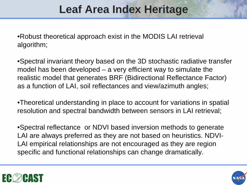
Leaf Area Index Heritage

•Robust theoretical approach exist in the MODIS LAI retrieval algorithm;

•Spectral invariant theory based on the 3D stochastic radiative transfer model has been developed – a very efficient way to simulate the realistic model that generates BRF (Bidirectional Reflectance Factor) as a function of LAI, soil reflectances and view/azimuth angles;

•Theoretical understanding in place to account for variations in spatial resolution and spectral bandwidth between sensors in LAI retrieval;

•Spectral reflectance or NDVI based inversion methods to generate LAI are always preferred as they are not based on heuristics. NDVI-LAI empirical relationships are not encouraged as they are region specific and functional relationships can change dramatically.

Surface Reflectances Process Overview• Global Land Survey (GLS) datasets are obtained from EDC

DAAC;

• Processing of GLS scenes using LEDAPS from GSFC for radiometric calibration and atmospheric corrections to derive first-pass surface reflectances (SRs);

• MODIS Collection 5 Landcover map downscaled to 30m as an initial input to LAI estimation;

• For continental US, 30-m NLCD landcover map is also used as input to LAI estimation.

• MODIS Collection 5 (MCD43A4) NBAR surface reflectance product utilized for testing reflectance consistency.

Spectral Invariants: Parameterization of Spectral Reflectance

• Radiative transfer theory of canopy spectral invariants provides the required Bidirectional Reflectance Function (BRF) parameterization via a small set of well defined measured variables;

• These variables specify the relationship between the spectral response of a scattering object bounded by a non-reflecting surface to the incident radiation at different spatial scales;

• Spectral invariant form of BRF can decouple the structural and spectral information.

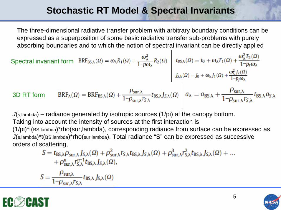
Stochastic RT Model & Spectral Invariants

5

The three-dimensional radiative transfer problem with arbitrary boundary conditions can be expressed as a superposition of some basic radiative transfer sub-problems with purely absorbing boundaries and to which the notion of spectral invariant can be directly applied

J(s,lambda) – radiance generated by isotropic sources (1/pi) at the canopy bottom. Taking into account the intensity of sources at the first interaction is (1/pi)*t(BS,lambda)*rho(sur,lambda), corresponding radiance from surface can be expressed as J(s,lambda)*t(BS,lambda)*rho(sur,lambda). Total radiance “S” can be expressed as successive orders of scattering,

Spectral invariant form

3D RT form

Spectral Invariant Approximation

6

xx

x

The total problem can be solved using the spectral invariant approximation

Biome specific LUTs can be efficiently created using the relation above

Adjustment for Spectral/Spatial Resolution

RatioIntegrate the “Ratio” for two different bandwidths corresponding to the red (580-680 nm) and NIR (725-1100 nm) bands.

Approximation to unity suggest the fact that differences in spectral characteristics between sensors can be solved by averaging the single scattering albedo over the sensor bandwidths

Adjustment for Spatial Resolution

LAI-NDVI relationships for different valuesof single scattering albedo

LAI Inversion Methodology

9

Each pixel can have a background ranging from dark soil to bright soils, and the LAI can vary over a range for each specific instance of background brightness

Reflectance Characterization at Landsat Scale

Reflectance characterization in the Red, NIR and SWIR plane

SWIR vs. Red scatter plot for different LAI ranges (y-axis: SWIR; x-axis: Red).

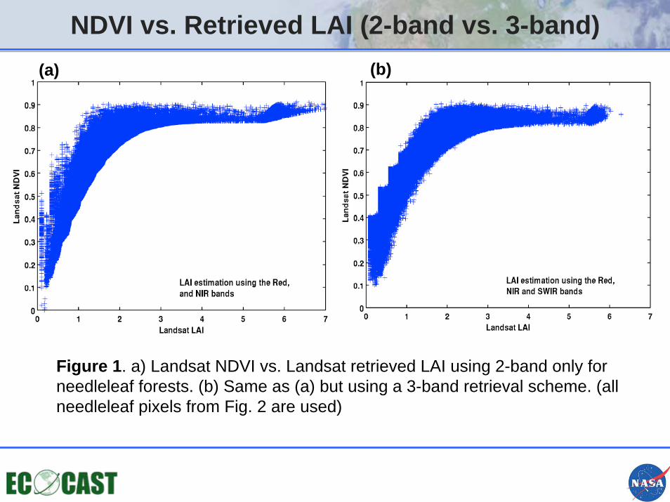
Figure 1. a) Landsat NDVI vs. Landsat retrieved LAI using 2-band only for needleleaf forests. (b) Same as (a) but using a 3-band retrieval scheme. (all needleleaf pixels from Fig. 2 are used)

NDVI vs. Retrieved LAI (2-band vs. 3-band)(a) (b)

Figure 2. (a) Landsat derived 30-m LAI map using the 3-band and 2-band retrieval scheme. (b) Landsat Quality layer displaying pixels that are retrieved using 3-band (green in color) and 2-band (yellow in color) (c) MODIS 1Km LAI map resampled to 30-m. (d) LAI difference map (Landsat – MODIS).

(a)

(c)

(b)

(d)

Landsat vs. MODIS LAI

Northern California Landsat Tile

Analysis at 30-m (Surface Reflectance and LAI)

13

Kansas Prairie (grasslands): Acquisition – 23rd July

Landsat NDVI MODIS NDVI

Landsat & MODIS Red/NIR scatter plot for grassland pixels

Landsat LAI MODIS LAI

LAI derived based on NDVI/ SR


14

Harvard Forest (B.D.F): Acquisition – 24th September



Landsat & MODIS Red/NIR scatter plot for B.D.F pixels


Lower LAI ? – What’s the reason

15

ΔN

IR

Δ Red

Δ = Landsat - MODIS

Direction {tan-1(ΔNIR/Δred)} of pixel differences in majority lies below the 45 degree angle – hits the lower LAI isoline

Polar plot showing the direction and magnitudeof reflectance differences for all B.D.F pixels


16

Canada (Boreas - needleleaf): Acquisition – 24th September



Landsat & MODIS Red/NIR scatter plot for B.D.F pixels



17

Harvard Forest (B.D.F): Acquisition – 24th September



18



19

Kansas Cropland/grassland : Acquisition – 23rd July


Analysis at 500-m (LAI)

20

Grassland/ Cereal cropsMODIS LAI Landsat LAI 2-band inversion

Landsat LAI Simple Ratio Based

21

Broadleaf Crops

Landsat NDVI


MODIS NDVI

22

MODIS LAI Landsat LAI 2-band inversion

Landsat LAI Simple Ratio Based

Analysis at 500-m (LAI)

Reflectance Analysis

23

NLCD Landcover

Analysis

24

• Analysis at 500m gives a clear conceptual framework for developing the LUTs – apply simple scaling relations to these LUTs and apply at 30-m;

• NBAR and Landsat reflectances seem to be really consistent at the 500m scale - Landsat reflectances at 30-m averaged to 500m are real averages;

• Downsampling to 30-m should be performed with caution –results can be wrongly interpreted in scaling physical quantities (e.g. reflectances and LAI) – MODIS reflectancesscaled to 30-m are simple replications and hence will preserve the same physical nature as in 500-m.

Analysis

25

• What are the implications in retrieving the LAI at 30-m? – first ever 30-m wall-to-wall leaf density map from Landsat, implications for accurately estimating biomass, high resolution GPP estimation (scaling climate variables of course);

• If reflectance signatures still show the high dynamic range in red reflectances, the LAI retrieved will still be smaller compared to LAI retrieved at any coarse resolution pixel –even after scaling and tuning the LUTs;

• This is the best we can do and developing the basis at 500-m, showing consistency with MODIS and then scaling it back to 30-m is a good feasible approach.

Activities

26

• LAI maps used by Martha at USDA for irrigation mapping;• LAI to be created for South East Asia (2005 and 2000) – Atul Jain’s

project;• USGS wants the LAI as a standard higher level product – so with

our new computing framework, we can blast through all the scenesand create a first version LAI;

• Current improvement strategies for landcover mapping – use best landcover wherever possible (e.g. NLCD for US);

• Canadian Remote Sensing guys, ISPRA (Italy) and Japan wants the LAI product once released;

• Validation work to start soon – database being built with all available LAI field data;

• Technical paper to be wrapped up by end of this year;• Next year activity involves refining the product algorithm from

validation exercise;• Atmospheric correction (esp. cloud correction) still to be improved;

Thanks to all of you for providing me all the help and necessary support at every stage in spearheading this project – This can’t be done alone !!

A Physically Based Approach in Retrieving Vegetation … · A Physically Based Approach in...

Documents

Transcript of A Physically Based Approach in Retrieving Vegetation … · A Physically Based Approach in...