A Phenomenological Approach To Artificial Jazz Improvisation

Manuel Ebert

A Phenomenological Approach to Artificial Jazz Improvisation

PICS

Publications of the Institute of Cognitive Science

Volume 1-2010

ISSN: 1610-5389 Series title: PICS Publications of the Institute of Cognitive Science Volume: 1-2010 Place of publication: Osnabrück, Germany Date: September 2010 Editors: Kai-Uwe Kühnberger Peter König Sven Walter Cover design: Thorsten Hinrichs

© Institute of Cognitive Science

Manuel Ebert

A phenomenological approach toartificial jazz improvisation

A thesis submitted in partial fulfillment of the requirementsfor the degree of Bachelor of Science

Department of Cognitive ScienceUniversity of Osnabruck

First Supervisor: Priv. Doz. Dr. Helmar GustSecond Supervisor: Prof. Dr. Bernd Enders

Submitted: May 23, 2009

Abstract

This thesis proposes a novel approach towards the design of artificially creativesystems based on a phenomenological account of human creativity and the anal-ysis of existing approaches towards the same task through the exemplary studyof artificial jazz improvisation. It will be argued that in symbolic approachestowards creativity, similarity measures between symbols play a vital role in themodelling of human phenomena. An implementation based on the concepts andmechanisms found through the analysis of existing systems will be given andevaluated with respect to the phenomenology of human jazz performances.

Acknowledgements

The author would like to thank his supervisors, Helmar Gust and Bernd Enders,for their support and patience in answering numerous methodological questions;Tilman Weyde of the City University London for the continuous correspondenceand Bob Keller at the Harvey Mudd College for the transcriptions of improvisa-tions he provided with Impro-Visor, without which this thesis would have takena lot longer.

Contents

1 Introduction 91.1 Introduction into the music theory of jazz music . . . . . . . . . 101.2 A phenomenological approach to musical improvisation . . . . . 11

1.2.1 Qualities and properties of human musicians . . . . . . . 111.2.2 Existing approaches towards artificial jazz improvisation . 12

1.3 Analysis of existing approaches . . . . . . . . . . . . . . . . . . . 17

2 Proposal of a new approach 192.1 On the role of similarity measures in creativity . . . . . . . . . . 192.2 Overview of the suggested system . . . . . . . . . . . . . . . . . . 202.3 Creation phase . . . . . . . . . . . . . . . . . . . . . . . . . . . . 20

2.3.1 Pattern acquisition and processing . . . . . . . . . . . . . 202.3.2 Rhythmic similarity measures . . . . . . . . . . . . . . . . 282.3.3 Melodic similarity measures . . . . . . . . . . . . . . . . . 31

2.4 Training phase . . . . . . . . . . . . . . . . . . . . . . . . . . . . 322.4.1 Finding walks through pattern space . . . . . . . . . . . . 332.4.2 Applying note-level rules . . . . . . . . . . . . . . . . . . 342.4.3 Learning from human feedback . . . . . . . . . . . . . . . 35

3 Discussion and Evaluation 373.1 Creativity in general . . . . . . . . . . . . . . . . . . . . . . . . . 373.2 Learning behaviour . . . . . . . . . . . . . . . . . . . . . . . . . . 373.3 Playing behaviour . . . . . . . . . . . . . . . . . . . . . . . . . . 393.4 Other limitations . . . . . . . . . . . . . . . . . . . . . . . . . . . 39

4 Conclusion and Outlook 41

Bibliography 41

List of Figures

1.1 Eight measures from “Take the A train” in a lead sheet and anactual performance . . . . . . . . . . . . . . . . . . . . . . . . . . 10

1.2 Examples of different genomes in GenJam . . . . . . . . . . . . . 131.3 The recurrent neural network used in CHIME . . . . . . . . . . . 151.4 A parse tree produced with Impro-Visor . . . . . . . . . . . . . . 16

2.1 Pseudo-code for creating new players . . . . . . . . . . . . . . . . 212.2 Number of frequent rhythmic fragments required for different cov-

erage thresholds on the data set . . . . . . . . . . . . . . . . . . . 242.3 Number of frequent melodic fragments required for different cov-

erage thresholds on the data set using different representations . 272.4 Distribution of note intervals on the data set . . . . . . . . . . . 272.5 Similarity of rhythms . . . . . . . . . . . . . . . . . . . . . . . . . 302.6 A depiction of the geometric distance metric . . . . . . . . . . . . 312.7 Similarities between melodic fragments . . . . . . . . . . . . . . . 322.8 Extrapolation of transition matrices . . . . . . . . . . . . . . . . 332.9 Pseudo-code of the training algorithm . . . . . . . . . . . . . . . 342.10 The user interface . . . . . . . . . . . . . . . . . . . . . . . . . . 35

3.1 A performance of “Anthropology” . . . . . . . . . . . . . . . . . 38

List of Tables

2.1 List of all tunes in the data set . . . . . . . . . . . . . . . . . . . 222.2 Distribution of chord extensions on the data set . . . . . . . . . . 232.3 Frequent rhythmic fragments on the data set . . . . . . . . . . . 252.4 Frequent melodic fragments on the data set . . . . . . . . . . . . 26

“Life is like music; it must be composed by ear,feeling, and instinct, not by rule.”

Samuel Butler

CHAPTER 1

Introduction

Many people are quite quick to judge computers and artificial intelligence whenit comes to how “human” modern AIs are, and many claim that AI will indeednever achieve human qualities as computers cannot feel or love or be creative;too often these deficiencies are then attributed to the absence of a “soul” or anyother alleged entity vague enough to resist a scientific approach. With no intentto engage in a philosophical debate about the nature of creativity here, I believethat there are computational models for what we call creativity (or at least forthose phenomena we attribute to creativity), and what’s more, that music is aparticularly good domain to study creativity with the use of computers; mainlyfor two reasons:

1. We have a fairly complete structured formalisation of music through tra-ditional notation and modern protocols and specifications such as MIDIand MusicXML. Similar formalisations exist for language (although theyusually can’t account for all irregularities), but painting and other visualarts are much harder to represent in a way that allows for extraction ofelementary features and components.

2. Elements of music usually have much less symbolic designation of thingsin the “real world”, which again does not hold for many visual arts orlanguage. Although many musical elements or phrases may be connectedto specific moods, the “meaning” of musical elements and thus the priorknowledge required to produce music is assumed to be less complex thanthat of e.g. paintings and poems.

Unfortunately, studies in artificial creativity up to now are little systematicas there are only few and very vague commonly accepted paradigms and groundfacts on which analysis and synthesis of creative systems is possible. This thesiswill therefore follow a phenomenological approach by first discussing a num-ber of qualities, properties and phenomena that human musicians show whenimprovising music and learning to improvise music and thereafter examine themechanisms of existing systems that bring about those properties in contrast tothose that do not.

Considering creativity as a problem solving task in the widest sense, thisthesis proposes that one of the essential features of creativity is to be able tojudge the similarity of solutions within the solution space, based on the similarityof their constituents, e.g. humans can address the similarity of two paintings bycomparing the colour palette, style of strokes, motives, arrangement of objects,lighting and so on. Moreover I will claim that without this ability, creativity aswe know it would not exists and any creative products had to be products ofchance and randomness.

The mechanisms discovered through analysis of existing systems along witha similarity relation on the basic constituents of music, melody and rhythm, willthen be used to propose a new approach towards artificial improvisation whichenables a system to learn by both listening and playing and furthermore develop

1 Introduction 10

a unique style based on different training samples and user feedback, and bemoreover able to improvise over previously unheard tunes. By implementing andtraining the system I will then aim to demonstrate that the proposed frameworkboth in theory and in practise exhibits the qualities and phenomena describedearlier on.

The thesis will conclude with a review of the existing approaches and compar-ison to the proposed one and will finally suggest extensions that might improvethe computational and aesthetic performance of the system.

1.1 Introduction into the music theory of jazzmusic

Jazz as a genre now spans over more than a century of constant change so thatmodern flavours such as smooth jazz, nu jazz and jazz pop have little or nothingto do with the roots of jazz such as 1890s ragtime or New Orleans and Dixielandin the first two decades of the past century. This thesis will therefore focus onthe principles of jazz music of the late 40s and 50s, namely bebop, hard bopand cool jazz. Despite their different acoustic qualities, they share the same“framework”: collective improvisations based on so-called lead sheets.

For those unfamiliar with music theory or jazz music, some of the understoodphenomena about such music will now briefly be explained from a computationalperspective. To start with, the very basic element of music are notes, whichcan be seen as triplets of pitch, volume and duration. Melodies are temporalsequences of notes (and rests) and chords are sets of simultaneously played notes.Lead sheets usually provide the melody of the tune and the chord structure. Thetask of bebop improvisation is to play notes in accordance to the chord structureof the lead sheet.

Dm7

!A7

"#G7

$C6

%&$$$' '$($ $$$$D9

$$ $)$C6

!C6 %$ !

Dm7

$G7

!D9

%&((a) The original lead sheet (The Real Book vol. 1)

!Dm7

!" !A7

# !!" !!!$5 !"!!% !!!G7

&!' !G7

!!!Dm7

!!! !C6% ! !"!!! !!!

!C6 "( ! !$ ) ! ! ! ! !! ! ! ! !

C6! ! !3

! ! !" * D9*! D9!

(b) Transcription of an improvisation by Harold Land

Figure 1.1: The first eight measures from “Take the A train” illustrate the dif-ference between what is written in a lead sheet and what is actually being played.

Most typical recordings in those styles then follow, according to Walker(1997), the same structure: first the soloist (typically a saxophonist or thepianist if there are no other solo instruments) plays the original tune with onlyminor variations. The next repetition of the chorus will feature the musicianplaying an improvisation over the chord structure of the tune that may have verylittle to do with the actual melody. Other musicians will then take their turnsin playing solos, or special structures such as “trading fours” (four measuresof an instrumental solo alternate with four measures of a drum solo, or morerarely, somebody else’s solo) will be played. Figure 1.1 depicts an excerpt froma lead sheet notation of a jazz standard and a transcription of an improvisation

1 Introduction 11

over this standard.It is noteworthy that sometimes accompanying musicians (e.g. the bass

player) were just given the chord progression of a tune and could play along.This works because the chords and the key define what sounds consonant orharmonic and what will be dissonant. Let’s have a short look at this by lookingat the seventh measure of the example. The key of the example is C major, thechords in this measure are C6 and then A7 (the tonic with added sixth and thenmajor tonic-parallel with seventh1). So for the first two beats, the chord tonesare C, E, G and A. Furthermore D, F and B will sound consonant as they arein the scale of a C major tonic, however the latter two will usually not be seenon a long on-beat note as they are only a semitone away from the chord tonesE and C and will therefore be likely to sound dissonant to the accompaniment.For the second half of the measure the chord tones are A, Cis, E and G; with B,D and Fis also belonging to the scale. All tones on full beats are chord or scaletones; the Fis on the second eighth serves as an approach tone to the followingG. By submitting to those rules the musicians can ensure that they will producea consonant sound although none of them knows what the others are going toplay next.

However, Ramalho and Ganascia (1994) noted that musicians will generallynot be able to justify all decisions they make that lead towards their actualimprovisation. The problem of filling the immense gap between the mere gridof chords and a well-sounding, interesting improvisations is what makes thestudy of jazz performance interesting for cognitive scientists.

1.2 A phenomenological approach to musicalimprovisation

1.2.1 Qualities and properties of human musicians

Usually the way things are designed heavily depends on the way the successof the design is going to be evaluated – an evaluation measures those criteriathat matter to the designer, hence the designer tries to build things in a waythat maximises the evaluation results. So instead of asking how to design asystem that can improvise bebop we could rather ask how such systems can beevaluated and adapt our design strategies accordingly. In the simplest case, onecould judge how musical or ‘jazzy’ output of a given system is. This, however,neglects the slightly different goals of different approaches and more importantlyrelies on rather subjective measures. We therefore propose to assess such asystem by which phenomena it could principally produce and what behaviour itusually shows. If we had a comprehensive list of behaviours and qualities that weloosely connect to people being creative, we could analyse existing system thatbring about those behaviours and phenomena and abstract the mechanisms thatare responsible for that very thing. If a system produces all the phenomena andbehaviours specified then it will be either indistinguishable from real creativity– regardless of any explicit definition of creativity – or the list is not complete.

On the following pages, I will state some behaviours and phenomena thatcan be observed in human jazz learners and performers and discuss their appli-cability to artificial learners and performers.

Creativity in general

Johnson-Laird (1988) notes that improvisation, being a creative task, is char-acterised by non-determinism and the absence of well-defined goals. However

1One can rightfully argue that the C6-A7 actually serves as a dominant-parallel and majordominant to the next Dm7 chord, but for our purposes we can ignore subtleties of functionalinterpretation (if jazz with its many minor sevenths doesn’t render functional interpretationuseless, that is - but that’s another debate).

1 Introduction 12

already twenty years ago there were, according to Taylor (1988), more than 60different models and definitions of creativity of varying explanatory depth andplausibility, and there is little evidence for any of them being the definite answerto the question of the nature of creativity, nor does it seem like there is any hopethat this question will be settled any time soon. In fact, many people believethat there can never be any scientific explanation of creativity2. This might wellbe a reason that the approaches to artificial improvisation covered in the nextsections (rightfully?) follow a strategy of forthright ignorance by simply disre-garding the terminological, psychological and modelling ballast that comes withthe fact that they are implementing a creative process. Having said that, thereare some observations on creativity that hold regardless of the model drawn onto explain these observations. Poincare (1913) remarked that “to create con-sists of making new combinations of associative elements which are useful” – thematter of association in creativity will be elaborated in section 2.1; particularattention should be paid to what exactly these “elements” consist of.

Learning behaviour

Most contemporary European jazz musicians received, at least for some time,a classical music education and have developed technical skills on one or moreinstruments before starting to play jazz3. Although they will be familiar with thescales that different chords provide, classically trained musicians will generallynot be able to come up with an innovative jazz improvisation if given a leadsheet, more likely will they, more or less, reproduce the melody with slightrhythmic variations of which they (intuitively) think that they might soundjazzy. Baker (1978) points out that Jazz musicians don’t learn by studying inconservatories but rather by listening and practising, and both depend on eachother: an experienced jazz musician will find different things in an improvisationhe listens to and incorporate that into his own style and repertoire than a novice.However at no point does a jazz learner sound “chaotic” or random – quite theopposite: if unsure what to play he will stick to more conventional licks.

Playing behaviour

Amongst the obvious phenomena of jazz music is that musicians can play andimprovise over almost any unknown tune if given a lead sheet. However afterhaving played a tune a few times musicians will sometimes stick to a certainimprovisation which they like most and will play that (with minor variations)in performances. During jam sessions or performances, musicians can respondto musical material played by other players to maintain a coherent style incollaborative improvisations, and even within a single improvisation there areoften motifs that are heavily repeated and referenced. Sloboda (1985) drawsour attention to the seemingly subtle phenomena that when playing, musiciansdon’t just decide “which note to play next” but rather decide on whole chunksof notes at once. Nonetheless, Widmer (2001, 2005) showed that – at least inclassical music – there are note-level rules that seem to be more or less innate topianists that determine micro-timing, accentuation and other note-level features;see section 4.

1.2.2 Existing approaches towards artificial jazz improvi-sation

In this section several existing systems that generate Jazz performances (or areclosely related to that task) will be introduced. The main focus is on different

2Which in most cases is a metaphysical stance based on the neglect and misunderstandingof what science and creativity are about rather than a conclusion based on the comprehensionand awareness of these very things.

3This doesn’t necessarily hold for performers of the ‘rest of the world’; particularly manyblack American performers in the 50s and 60s were raised with jazz.

1 Introduction 13

ways to represent and encode music, but the algorithms used to produce actualmusic from what is represented in the systems will also be touched on. Thisoverview is far from being comprehensive and the reader is encouraged to lookinto the work of Dahlstedt and Nordahl (2001) on evolutionary “living” melodiesand and the statistical approaches of Allan and Williams (2005) and Thom(2000) (the latter with a focus on solo trading) which will not be covered in thissection. However I do think that this selection of systems gives a good insightinto the kind of work and different approaches towards the aforementioned taskand will serve as examples to describe common patterns and issues.

Genome-based representations

Similar to Dahlstedt and Nordahl (2001) and Papadopoulos and Wiggins (1998),Biles (1994) represents melodies in artificial genomes. In one population eachindividual genome encodes one measure of music by specifying one of 16 possibleevents for each eighth beat of the measure: 1 to 14 denote the onset of one offourteen different tones (which are relative to the scale the current chord pro-vides, i.e. a 3 would be an E if the chord was C6 but a Cis if the chord was A7),0 denotes a rest and 15 a “hold” – which extends the duration of the previousnote or rest. Thus every genome of a measure individual is 32 bits long. Ina second population the genomes encode a sequence of four individuals of themeasure population (cf. figure 1.2); as this population is limited to 64 individ-uals, every phrase genome will be 24 bits long. Once two suitable populationsare bred, GenJam builds an improvisation using a chord progression file (whichalso includes MIDI sequences for bass, drums and piano) and selecting individ-uals from the phrase population which then each supply melodic material forfour measures. The relative tones encoded by the measures are translated intoabsolute tones by built-in scales for the aligned chord in the chord progressionfile and sent to a MIDI device. The listener can give feedback to the system bytyping g for good or b for bad (even several times), which modifies the fitnessvalues of the current phrase and measure individuals.

#23 -12 57 57 11 38

(a) Phrase Population

#11 6 9 7 0 5 7 8 7 5

# 38 -4 7 8 7 7 15 15 15 0

# 57 22 9 7 0 5 7 15 15 0

(b) Measure population

Figure 1.2: Examples of genomes of individuals in (a) the phrase- and (b) mea-sure population and their fitness in GenJam (adapted from Biles (1994)).

If the system is in learning mode, the phrase individuals are selected at ran-dom while in demo mode phrases are selected by a tournament process whichnot only takes the fitness of the phrases into account but also the fitness of con-stituent measures. In a third mode, called breeding mode, half of the populationis replaced by mutated offsprings after each solo. The selection process worksby randomly grouping the individuals into families of four and then keeping thetwo family members with the highest fitness as parents and replacing the othertwo by offsprings of those parents. The children are created by first applying arandom single-point crossover to the parents’ genomes (i.e. each child’s genomewill be identical to its fathers genome up to some point and from there on iden-

1 Introduction 14

tical to its mother’s genome). One of the two children of a family will be keptintact, the other one mutated by one of the following musically “meaningful”mutation operators:

(a) Reversing the notes (blocks of 4 bits)

(b) Rotating the notes by a random number of notes

(c) Inversion

(d) Sorting notes in ascending order (rests and holds are not affected)

(e) Sorting notes in descending order (rests and holds are not affected)

(f) Transposing notes by a random number ∈ [1, 14]

Phrases are mutated by applying one of the following operators:

(a) Reversing the measures (blocks of 5 bits)

(b) Rotating the measures by a random number of measures

(c) Genetic repair: replace measure with worst fitness by random measureindex

(d) Super phrase: replace all measures by winners of four three-measure tour-naments

(e) Lick thinner: replace a random measure by the one that occurs mostoften in the phrase population

(f) Orphan Phrase: replace all measures by winners of four three-measuretournaments. where the winner is the measure that occurs least frequentlyon the phrase measure (maintains genetic diversity)

Two major differences to plain genetic algorithms (i.e. Mitchell (1996)) are ob-vious: firstly, GenJam uses the whole population to create a performance andnot just the fittest. Secondly, the mutation operators are not “dumb” [sic] withrespect to the structures they alter. Other remarkable features of GenJam in-clude that the chord progression file can define a swing rhythm by which twoquavers will sound as a triplet of a crotchet and a quaver. Furthermore, a col-laborative mode exists in which GenJam will listen for MIDI input, convert thisinput into measure and phrase individual, apply the above mentioned geneticoperators and play the results – which resembles “trading fours”.

Neural networks

Franklin (2001) utilises a recurrent neural network that can memorise threedifferent melodies for her CHIME framework (“computer human interactingmusical entity”). Recurrent networks differ from plain vanilla networks in thatthe output is used as part of the input; the learning data are then usuallysequences. This has the effect that the previously seen data sample can beused as the context of the current sample. The network in use is depicted infigure 1.3. The exact network topology is as follows:

• Three plan input units. They indicate the index of one of the threemelodies that are learned using 1-of-N encoding (1-0-0 for 1, 0-1-0 for2 etc.)

• Twelve chord input units; each unit corresponds to one chromatic noteand is set to 1 if that note is part of the input chord.

1 Introduction 15

• 26 context input units that have recurrent feedback connections from theoutput units. When propagating the error, a method called teacher forcingis used to update the self-connecting weights with the target output ratherthan the actual output.

• 50 hidden units (this number was experimentally derived)

• 26 output units, consisting of 24 units representing the chromatic notes oftwo octaves, one representing a rest and a new note indicator. Among thefirst 25 outputs, the one with the greatest value is selected as the nextnote that is being played; if the new note indicator is above a certainthreshold a new note onset is played, otherwise the last note is being heldfor another time step.

• The learning rate was set to ε = 0.075

Figure 1.3: The recurrent neural network used by Franklin (2001) in phase 1.

The network was then used to memorise three songs; each song contained192 semiquavers and was presented to the network 15.000 times until the songsas replayed by the network were “easily recognised”. After training, the networkcan be used to play trading fours with a human player: the recurrent connectionsare removed and all plan inputs set to 1. Each time the human has playedfour measures, the recorded notes of the human solo are used as inputs for thenetwork, and together with the weights learned from the three songs the networkproduces a melody of its own – though the network can only produce as muchnovel music as it receives input stored from the last four measures the humanplayed.

Franklin extended the network by transforming it into an actor-critic rein-forcement learner with human input, which will not be covered here due to spacelimitations. Also, we would like to draw the reader’s attention to the work ofEck and Schmidhuber (2002a,b) which uses long short-term memory (LSTM)networks to allow for the inclusion of a longer temporal context into the input.

1 Introduction 16

Rule-based approaches

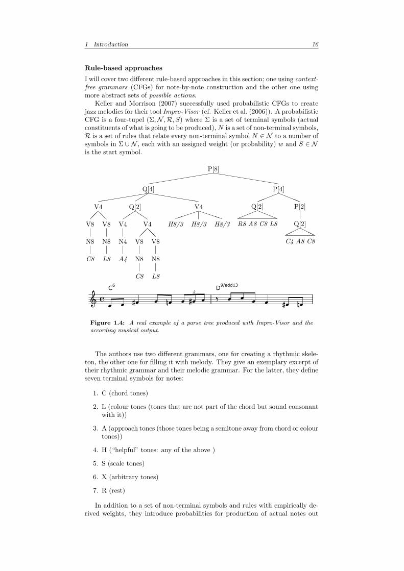
I will cover two different rule-based approaches in this section; one using context-free grammars (CFGs) for note-by-note construction and the other one usingmore abstract sets of possible actions.

Keller and Morrison (2007) successfully used probabilistic CFGs to createjazz melodies for their tool Impro-Visor (cf. Keller et al. (2006)). A probabilisticCFG is a four-tupel (Σ,N ,R, S) where Σ is a set of terminal symbols (actualconstituents of what is going to be produced), N is a set of non-terminal symbols,R is a set of rules that relate every non-terminal symbol N ∈ N to a number ofsymbols in Σ ∪ N , each with an assigned weight (or probability) w and S ∈ Nis the start symbol.

P[8]!!!!!!!!!!""""""""""

Q[4]!!!!!!!!##""""""""

V4$$%%

V8

N8

C8

V8

N8

L8

Q[2]&&''

V4

N4

A4

V4$$%%

V8

N8

C8

V8

N8

L8

V4((((

))))H8/3 H8/3 H8/3

P[4]****

++++Q[2]

***+++

R8 A8 C8 L8

P[2]

Q[2],,,---

C4 A8 C8

! "#$ " " ""C6

" ""%D9/add13

&"# ! "" " 3

!" "

Music engraving by LilyPond 2.10.33—www.lilypond.org

1

Figure 1.4: A real example of a parse tree produced with Impro-Visor and theaccording musical output.

The authors use two different grammars, one for creating a rhythmic skele-ton, the other one for filling it with melody. They give an exemplary excerpt oftheir rhythmic grammar and their melodic grammar. For the latter, they defineseven terminal symbols for notes:

1. C (chord tones)

2. L (colour tones (tones that are not part of the chord but sound consonantwith it))

3. A (approach tones (those tones being a semitone away from chord or colourtones))

4. H (“helpful” tones: any of the above )

5. S (scale tones)

6. X (arbitrary tones)

7. R (rest)

In addition to a set of non-terminal symbols and rules with empirically de-rived weights, they introduce probabilities for production of actual notes out

1 Introduction 17

of each of the above mentioned symbols that depend on the chord that is be-ing played. Also certain parameters for non-terminal symbols are used whichstrictly speaking are not context-free anymore, but ensure that the sequence hasa fixed length, that approach tones are always succeeded by chord tones etc.

The melodies created by their grammar are mostly consistent with whatyou expect from jazz melodies, and Keller (a part-time jazz teacher) judges thebetter results to be of quality comparable to college-level jazz students. Anexample is given in figure 1.4.

Ramalho and Ganascia (1994) in contrast define more abstract rules andconstituents in their PACT framework to make improvisation a classical prob-lem solving task. First, they introduce two basic components of their system:potential actions (PACTs) and musical memory. A potential action may bethought of as the intentions musicians have during a performance. The authorsdistinguish between PACTs with a low level of abstraction that directly influencerhythm, pitch and amplitudes of notes (such as “play loudly”) and highly ab-stracted PACTs like “play the same lick, but transposed one semitone higher”.Furthermore they distinguish procedural PACTs (such as “play an arpeggio”)and property-setting PACTs, e.g. “play bluesy”. PACTs may combine to a newPACT, which entails two important properties of PACTs:

1. Playability : the reciprocal of the amount of information that’s missing toactually play the PACT

2. Combinability : whether PACTs can combine to produce more playablePACTs and to exclude contradicting PACTs (such as “play loudly” and“play quietly”).

The problem solving task is then characterised by starting with an empty setof bars and possibly a set of abstract PACTs and the goal is to fill the bars withnotes through combining PACTs while obeying the constraint of combinability(“the goal is to play!”).

As there is no guarantee that a set of PACTs contains all information thatis required to produce a full melody (in other words, that it is playable) theauthors introduce musical memory. While the PACTs described above weremanually implemented by formalising expert knowledge of jazz improvisation,the musical memory represents what a musician learns by listening to jazz music.Hence the musical memory contains (typically low-level) PACTs that have beenautomatically obtained (though with human guidance) from transcriptions ofreal improvisations such as rhythm patterns, melody fragments etc.

A reasoner is then used to produce unique playable PACTs based on a chordgrid and the reasoner’s mood. The mood is controlled by a perception modulethat allows interaction of the external environment and the musician, howeverthe authors are quite unspecific as to how exactly this module works. Similar toa planning system, the reasoner uses three operators: combine to combine twocompatible PACTs into a new one, delete to resolve incompatibilities betweenPACTs and add to include PACTs from the musical memory that provide theinformation missing to produce a unique playable PACT.

1.3 Analysis of existing approaches

To summarise section 1.2.1, (most) human jazz music is characterised by thefollowing features:

(a) Non-determinism

(b) Absence of well-defined goals

1 Introduction 18

(c) Combination of associative elements

(d) Learning process starts with small variations of known tunes

(e) Learning by listening and playing

(f) Some known rules (e.g. chord scales)

(g) Musicians play by chunks of notes rather than note-by-note

(h) Possibly note-level rules for expression, articulation, timing etc.

(i) Musicians can respond to musical input

(j) Use of repeating motifs

(k) Musicians can improvise over previously unknown songs but will alsoretain good improvisations for known songs.

By comparing the approaches described above (and the musical output pro-duced by their implementations) it can be seen that despite the diversity ofrepresentations and algorithms used, the same mechanisms and underlying as-sumptions are used to bring about these properties in different systems:

(c) Although this phenomenon offers a rather wide range for interpretationdepending of what one considers to be an associative element, the mostconspicuous elements are those on the level of the “chunks” of notes men-tioned in (g). GenJam provides a good example of how to engender thatvery effect by representing chunks as individuals of the measure populationand the association of chunks by the phrase population (whether a mea-sure is a good approximation to a chunk will be discussed in section 3.4)

(d, e) Systems that can learn by listening (supervised learning) before receivinghuman feedback learn a lot faster (in real time, not necessarily in itera-tions) and will have a solid basis before presenting material to the humanmentor. This can be nicely seen by comparing GenJam with CHIME (withthe reinforcement extension).

(f) Most systems map the generated pitches to the scale provided by thecurrent chord to ensure some harmony. Unfortunately there seems to beno study on how it affects the learning behaviour if the chord scales haveto be learned as well; and it is hard to isolate this factor from systemsthat do (ie. CHIME). Nevertheless, we can assume that this is an usefulway of incorporating prior knowledge into the system.

(g) Approaches that represent knowledge using ‘patches’ of music like GenJam(where these patches are the individuals of a population) or the PACTframework tend to produce music with more local coherence than ap-proaches that will produce music one note after another (i.e. CHIME orstochastic approaches using Markov models such as Allan and Williams(2005)).

(h) Note-level rules for timing might be conceivable for approaches that workon note-level such as CHIME or HMMs, however Widmer’s work mightbe used as an add-on layer to patch- or pattern-based approaches as well.

(i) In order to respond to human musicians, musical input has to be parsedand transformed to the representation the learner uses for its own musi-cal material. Therefore it must be possible to reverse the output (actualmusic) to the inner representation of musical properties; at least to thelevel from where musical operators can be applied. It is not immediatelyclear how this can work in grammar-based approaches (although creating

1 Introduction 19

a parse-tree and modifying it might work, however the cognitive motiva-tion for this approach is questionable) and even more difficult when usingstochastic models on note-level basis.

(j) The intentional use of repeating motifs is, by definition, impossible forcontext-free grammars and is left to chance in all other systems with thenotable exception of the PACT framework that might indeed have context-sensitive structures.

(k) All the approaches described above lack the ability to generate unique andrecognisable solos for different tunes without having been trained for eachnew tune separately; or at least none of them describes how tune-specificknowledge could be incorporated into their representation and algorithms.

CHAPTER 2

Proposal of a new approach

Based on the findings obtained through the deconstruction of previously pre-sented systems, this section will expound the systematic assembly of the exposedmechanisms into a system that displays the traits and qualities of human jazzperformances and performers inspected in the previous chapter.

2.1 On the role of similarity measures in cre-ativity

It can hardly be argued that humans do not have an intuitive sense of sim-ilarity, no matter whether it is innate or culturally dependent, even if theycannot verbalise it. This sense of similarity seems to be an intrinsic propertyof creativity, as without it any product of creativity would be unrelated to anypreviously existing things, and although such a product may be the result ofan analytic process this process will therefore lack the phenomenology of cre-ativity. However, there are also formal arguments for the use of similarity increative processes (and in fact for a lot of problems related to search and plan-ning in “good old-fashioned” artificial intelligence): assuming that memoriesand ideas are not explicitly stored in our brain as discrete entities but ratheras implicit properties of the structure of the brain, e.g. synaptic connections,studies on artificial neural networks suggest that the structure bears informationon the correlation of afferent and efferent signals, i.e. the input and the outputof networks (which in the case of the brain correspond to external stimuli andmemories that are invoked by those stimuli). Examples of such networks areHopfield networks (which are explicitly trained with the correlation betweentraining patterns) and Multi-Layer perceptrons. This process of correlating in-put with output by means of previously learned correlation may be thought ofas association and is also an important mechanism in dealing with incompleteknowledge (which, for human beings, may be the case almost every time and onevery level of understanding). In systems where information is explicitly stored,such as it is the case in many classical applications of artificial intelligence how-ever, there is no or only marginal knowledge of how these bits of informationare correlated. Similarity measures are one way to allow associative processesand processes working on incomplete knowledge in those systems. One mighteven claim that similarity is merely another word for the way information isstored in our associative memory, which also explains why we can easily breakdown the similarity of two objects to the similarity of their components and thecomponents’ components respectively.

In the following sections, a novel approach to artificial improvisation basedon the concept associative components and similarity as means of associationbetween components will be described.

2 Proposal of a new approach 21

2.2 Overview of the suggested system

The framework proposed can be split into two phases; the creation phase andthe training phase. In the creation phase, transcriptions of solos are read andfragmented and a player object is instantiated with the information gained fromthose transcriptions. In the training phase, an instantiated player may use thepreviously gained knowledge to perform new solos and gain reward or punish-ment from the user which is then incorporated into its prior knowledge.

The aim of the creation phase is to estimate all probability distributions suchthat the conditional probability of any melodic and rhythmic fragment beingplayed next given which fragments are being played right now can be computed:

Pr(rj ,mq|ri,mp) ≈ Pr(rj |ri) · Pr(mq|mp) · Pr(rj ,mq) (2.2.1)

for all rhythmic fragments ri, rj ∈ R, the set of frequent rhythmic fragmentslearned by the player, and accordingly mp,mq ∈M , the set of frequent melodicfragments learned by the player. Equation 2.2.1 is the so-called performancetask, along with the algorithm that combines a rhythmic with a melodic frag-ments. However, we would like to include specific knowledge for different tunesΘ ∈ T such that the probabilities described in equation 2.2.1 change accordingto the tune over which the solo is being performed. Formally, this is done byaltering equation 2.2.1:

Pr(rj ,mq|ri,mp,Θ) ≈ Pr(rj |ri) · Pr(mq|mp) · Pr(rj ,mq)·Pr(rj |ri,Θ) · Pr(mq|mp,Θ) · Pr(rj ,mq,Θ)

(2.2.2)

We will call this the layered performance task, as we can think of tunes asadditional layers of probabilities. The conditional probability distribution canbe thought of as being a Markov model of order one, and that mere thoughtprovides us with a great variety of tools for dealing with Markovian decisionprocesses, e.g. from computational linguistics. However, given the nature ofthe data from which the probability distributions are estimated, they can alsobe thought of as resembling an associative process that lets musicians think ofthe next fragment to play based on what they are playing right now. To avoidprecision issues in floating point operation when dealing with many fragments(and thus very small probabilities), it might be necessary to operate on the sumof logarithms of probabilities instead of the product; however in tests with upto forty rhythmic and melodic fragments no visible errors occurred.

The creation algorithm is sketched in figure 2.1, further explanations aregiven in the subsequent sections. Everything is implemented in Python 2.5 1

(see Van Rossum and Drake (2003) for details) with the help of the PyGamemodule2 for audio output.

2.3 Creation phase

2.3.1 Pattern acquisition and processing

The data set in use is based on the transcriptions of improvisations that shipwith Impro-Visor 3.39 (see Keller et al. (2006)). A detailed listing of tunes usedis given in table 2.1. All transcriptions used are in 4/4 rhythm and meant tobe played in a swingy style (two quavers becoming a triplet of a crotchet anda quaver). Table 2.2 shows the distribution of chords; as the frequencies of allchord extensions that do not alter the scale given by the chord root (e.g. Xm7

in contrast to Xm7b5, which introduces the flat fifth into the scale) already sumsup to 0.927 we can assume that in most cases the distinction between major

1Available at http://www.python.org/2Available at http://www.pygame.org/

http://www.python.org/

http://www.pygame.org/


1. require transcription files

2. notes ← read transcription files

3. N(t)← calculate conditional note functions from notes

4. F ∗ ← fragmentise notes

5. R∗ ← get rhythmic fragments from F ∗

6. M∗ ← get melodic fragments from F ∗

7. R ← select frequent rhythmic fragments from R∗

8. M ← select frequent melodic fragments from M∗

9. R ← count rhythmic transitions of R in R∗

10. M ← count melodic transitions of M in M∗

11. A ← count alignments of R,M in R∗,M∗

12. S(R) ← calculate rhythmic similarities in R

13. S(M) ← calculate melodic similarities in M

14. R ← extrapolate R using S(R)

15. M ← extrapolateM using S(M)

16. A ← extrapolate A using S(M), S(R)

17. R,M, A ← thin R,M, A

18. create new player with R,M, R,M, A

Figure 2.1: Simplified pseudo-code for creating new players.

and minor chords is enough to determine whether a given note is out of scale ornot.

The transcriptions are formatted by pairs of keys and arguments, surroundedby round brackets, e.g. (composer Charlie Parker). The keywords are title,composer, key to identify the key of the solo, e.g. Bb, choruses followed bya number that indicates how many repetitions of the chorus are transcribed,chords and notes. The argument to chords is the chord sequence for this solo.Measures are separated by the pipe character, and each measure can containone, two or four chords from the list of chords give in table 2.2 (along with aroot for the chord) or the slash character that repeats the previous chord. Thenotes keyword expects an argument that lists all notes of the solo separated bywhite spaces. Each note has to match the following expression:

([a-g][b#]?|r)(\+*|\-*)(\D(\+\D)*)?

with \D set to

(1|2|4|8|16|32)(\.|/3)?

The first part, ([a-g][b#]?|r), identifies the note with optional accidental or arest, each + or - in ([\+]*|[\-]*) increases or decreases the octave of the noteby one (that is, adds 12 or −12 to the pitch), and the last part identifies theduration of the note, which has to start with a number, followed by an optional. to identify a dotted note or an /3 to identify a triplet, optionally followed by


an unlimited number of duration definitions joined by the + character which willbe added to the notes duration. If no duration is specified, the duration will beset to one eighth. In the process of reading transcription files, the duration willbe converted to an integer such that a breve has the value 96 (i.e. the shortestpossible duration is 32/3 which has value 1) and the pitch will be converted toan integer such that A440 will have a value of 48.

Name Artist MeasuresAnthropology Charlie Parker 60Bye Bye Blackbird Ray Henderson 31Byrd Like Freddie Hubbard 107Cheryl Charlie Parker 58Dewey Square Charlie Parker 30Groovin’ High Dizzy Gillespie 17Laird Baird Charlie Parker 36Moment’s Notice John Coltrane 41Moose The Mooche Charlie Parker 30Now’s The Time3 Charlie Parker 58Now’s The Time3 Charlie Parker 90On Green Dolphin Street Unknown 57Ornithology Charlie Parker 31Scrapple From the Apple Charlie Parker 30Yardbird Suite Charlie Parker 31

Table 2.1: Tunes in the set of transcriptions used by Impro-Visor, adding up toa total length of 707 measures.

Transcription files can be read, parsed and transformed to a pattern inven-tory using the Python script

$ ./run.py create input file1 [input file2 ...]

With the -r-argument, a profile can be specified (as defined in profiles.conf);if no profile is given the user will be queried with a list of available profiles. Aprofile is a set of parameters that override the standard parameter set which isspecified as the default-profile in profiles.conf. With the optional argument-n a name can be set for the player that is about to be created, furthermore-d turns on the debug mode. This will run the algorithm that is sketched infigure 2.1 and save the player into the players folder, along with a .statsfile which includes everything that was learned during creation and to whichchanges that are made during the training phase will be appended.

Then in step 3 of the creation algorithm, the conditional note function dis-tribution N : N→ R4 is calculated from the notes read in the previous step suchthat N(t) is a four-tuple4 of probabilities for a note at onset t of a fragmentbeing a chord tone, colour tone, approach tone or arbitrary tone (x) (cf. Keller(2007)):

N(t) = (Pr(h|t),Pr(c|t),Pr(a|t),Pr(x|t))

Thereafter, the data set will be fragmentised in step 4, and this sequence ofmusical fragments will converted into a sequence of corresponding rhythmicand melodic fragments afterwards. Fragmentation simply means splitting thesequence of notes on the data set into parts such that the notes and rests inevery part sum up to the same constant value. It is usually said that jazz

3The first version was played in F major and contains six choruses, the second version wasplayed in G major over eight choruses.

4Although rest is another note function, it will not be covered by this probability distri-bution for reasons that will become evident in section 2.4.2.


Chord Frequency ΣX7 0.476 0.476Xm7 0.241 0.717XM7 0.092 0.810X 0.050 0.860X6 0.039 0.899X7alt 0.034 0.934Xo7 0.016 0.950Xm 0.012 0.963Xm7b5 0.011 0.974X7b9 0.007 0.985X9 0.007 0.983Xm6 0.003 0.996XM6 0.002 0.999X7#9 0.001 1.000

Table 2.2: Distribution of chord extensions on the Impro-Visor data set, summedover all possible roots. The X is a placeholder for different chord bases.

musicians think about three seconds in advance when deciding what to playnext; with a typical tempo of 160 beats per minute in bebop, that adds up to twomeasures. However for data analytical reasons all experiments described herewere performed using fragments of half a measure’s length and a full measure’slength – we will see in the following sections why this is beneficial. Fragments ofvariable length (i.e. the data set being split by a criterion different to fragmentlength) are conceivable, too, and this point will be discussed later on.

Rhythmic representation and segmentation

As said in section 1.1, a melody is defined as a sequence of triples of pitch,volume and duration, and each fragment that is extracted from the data set is amelody in this sense such that all durations of this sequence sum up to a givenlength (with rests included as notes with the special pitch of −1). Simply put,a rhythmic fragment is a sequence of notes and rests without pitches. As thedata set in use does not give any volume information of the notes a rhythmicfragment can be represented as a set of pairs of onset on duration (where 96 isthe duration of a full measure).

Although a data set of some 800 tokens seems utterly undersized to representall aspects of bebop improvisation, we can show that certain characteristics usedby the system proposed are invariant to the size of the data set: the number ofdistinct tokens that are minimally required (i.e. the number of most frequentfragments) to cover a certain fraction of the data set only depends on the lengthof the token and the fraction to be covered, given the data set is sufficiently large.This can be shown by starting with a subset of the data set of length one andincrementally increasing the subset. For every step, it was calculated how manydistinct fragments were required for covering the different fractions of that dataset of this size. The results can be seen in figure 2.2: apparently the minimalnumber of fragments that cover specific fractions of the data set converges to afixed point. These numbers will be used as references in initialising the system’sinventory: smaller numbers (i.e. less fragments) will yield more robust results,however larger numbers may yield aesthetically more interesting results.

Table 2.3 shows the twenty most frequent rhythmic fragments R for dif-ferent fragment sizes on the full data set R∗ which are selected in step 7 inalgorithm 2.1.

Step 9 in algorithm 2.1 then estimates the transition probabilities from and


0 500 1000 15060

50

100

150

200

250

300

350

Size of data set (fragments)

Min

imal

num

ber o

f dist

inct

frag

men

tsre

quire

d fo

r cov

erag

e of

n%

(a) Fragment length = 1/2 measure

0 200 400 600 7530

50

100

150

200

250

300

350

Size of data set (fragments)

Min

imal

num

ber o

f dist

inct

frag

men

tsre

quire

d fo

r cov

erag

e of

n%

(b) Fragment length = 1 measure

25% coverage50% coverage66% coverage75% coverage90% coverage

Figure 2.2: Number of most frequent rhythmic fragments required for coveringdifferent fractions of the (rhythmic) data set for different data set sizes and (a)fragments of half a measure and (b) fragments of a full measure’s length. Thisfigure depicts the average over ten randomisations of the data set (ie. randompermutations of the ordering of fragments), however the results for random per-mutations of tunes or no randomisation at all are almost the same.

to each of the fragments selected in step 7 such that for all ri, rj ∈ R:

Pr(rj |ri) =CR∗(ri, rj)CR∗(ri)

where CR∗(ri, rj) is the number of occurrences of the sequence (ri, rj) in therhythmic data set R∗. These transition probabilities are stored in a transitionmatrix R such that Ri,j = Pr(rj , ri).

According to some similarity measure σ (which will be described in sec-tion 2.3.2), a similarity matrix S(R) will be computed in step 12 of the creationalgorithm such that S(R)

i,j = σ(ri, rj). This similarity matrix is used to extrapo-late unseen rhythmic transitions in step 14 using the nearest neighbour heuristicand the rhythmic extrapolation factor κr ∈ [0, 1] that controls the weight of ex-trapolated values compared to actually seen transitions. This is done by settingany unseen transitions to the probability of the transition with the most similarconditional multiplied by the similarity of the two conditionals and κr:

Ri,j =

{κr · Rk,j · S(R)

k,i such that k = arg maxk

S(R)k,i if Ri,j = 0

Ri,j else(2.3.1)

Other ways of extrapolating missing values are certainly possible and shouldbe investigated. After performing equation 2.3.1 in step 14 each row has to benormalised again so as to add up to one:

Ri,j ←Ri,j∑|R|

1=k Ri,k

Finally, the extrapolated rhythmic transitions will be thinned in step 17 by arhythmic thinning factor δr such that 0 ≤ δr ≤ 1, which means that a fractionδr of each transitions probability will be evenly distributed over all transitionprobabilities with the same conditional.

Ri,j ← (1− δr)Ri,j +1|R|

|R|∑k=1

δrRi,k

As each row in R adds up to one this simplifies to

Ri,j ← (1− δr)Ri,j +δr|R|

(2.3.2)


Thinning is an important mechanism for the performance task 2.2.2 as it reg-ulates the “importance” of e.g. rhythmic transitions over melodic transitions– the more homogeneous one of the factors becomes, the less influence it willhave on the final conditional probabilities from which a next pair of rhythmicand melodic fragments will be selected, up to the extreme of δr = 1 at whicha matrix will be entirely homogeneous after thinning and thus have no impacton the decision process. Thinning factors for rhythmic and melodic transitionmatrices as well as the alignment matrix can be set in profiles.conf.

Melodic representation and segmentation

Section 2.3.1 described the representation of and calculations done with rhyth-mic fragments. Although steps 7, 9, 14 and 17 of the creation algorithm 2.1 canbe directly applied to melodic fragments as well (which is done in steps 8, 10, 15and 17, respectively), it is not immediately apparent how to represent melodicfragments.

As opposed to rhythmic fractions, where we have seen that a fairly smallnumber of distinct fragments accounts for most of the rhythms seen on the dataset, considerable abstraction from the surface form of melodies is necessary toproduce similar effects for melodic fragments. Simply encoding the absolutepitch of each note (whilst ignoring onset and duration as these are encoded in

Rank Rhythm f∑

rf

(1) !42 ! ! ! 0.292 0.292

(2) !

42 0.162 0.454

(3)!

"!!

42 0.031 0.485

(4)"!!

42 # 0.029 0.513

(5) ! !

"!

42 ! 0.028 0.542

(6) !!42 ! 0.025 0.566

(7) 42 !!# 0.023 0.590

(8) #42 ! ! 0.020 0.610

(9) ! !42 !!

3

! 0.019 0.629

(10) 42 ! # 0.019 0.648

(11) !! ! !!!42 !! 0.015 0.664

(12) 42 # ! 0.015 0.678

(13) 42 !

3"! !! ! 0.013 0.692

(14) ! !!42 0.013 0.704

(15) ! !

3

! !42 ! 0.013 0.717

(16) !

"!! !

42 0.010 0.727

(17) !!!42 !

3

! ! 0.009 0.737

(18) !!

""

42 !! 0.009 0.746

(19) ! !!

42 0.009 0.755

(20) !! !42

"

0.009 0.765

Rank Rhythm f∑

rf

(1) !! !" ! !!! ! 0.141 0.141(2) !" 0.089 0.230

(3) ! !" !!! 0.015 0.244

(4) ! !

3

!! !!! !" ! 0.015 0.259

(5) " !!!!

"

0.009 0.268

(6) " ! !# ! !

"!! 0.009 0.278

(7) " !! ! !! ! ! 0.009 0.287

(8) " ! !!! 0.009 0.296

(9) !!

3

!!" !!! ! !

"

0.009 0.305

(10)"!!" # ! 0.008 0.313

(11) ! !!! !" ! ! !! !!! ! !! ! 0.008 0.321

(12) " ! !! ! ! # 0.008 0.329

(13) !" !! ! ! 0.008 0.337

(14) ! !" ! !! !

"! ! 0.008 0.345

(15) !! !" 0.008 0.353

(16) ! ! !!" !! !!

3

! 0.008 0.361

(17) !" !! !! !! 0.007 0.368

(18) ! ! !

3

!" !! ! ! !! 0.007 0.375

(19) !!! ! !! !!!

"" ! 0.007 0.381

(20) " ! ! !! ! !! 0.007 0.388

Table 2.3: The twenty most common rhythmic fragments for (a) a fragment size ofhalf a measure and (b) a full measure, their frequency on the data set (occurences oversize of the data set) and the coverage (accumulated frequencies over all fragments ofequal or lower rank). In the former case, 172 distinct fragments can be found on thedata set, and it is evident that only about ten percent of the fragments account for twothirds of the whole data set. In the latter case, there are 394 distinct fragments.

Melodic representation and segmentation

2.3.2 Rhythmic similarity measures

Necessary qualities of rhythmic similarity

Existing approaches

Evaluation of approaches

2.3.3 Melodic similarity measures

Necessary qualities of rhythmic similarity

Existing approaches


2.3.4 Application of similarity measures

2.3.5 Melodic extrapolation

2.3.6 Finding walks through pattern space

2.3.7 Applying note-level rules

2.3.8 Learning from human feedback

16

Table 2.3: The twenty most common rhythmic fragments for (a) a fragment sizeof half a measure and (b) a full measure, their frequency on the data set (occur-rences over size of the data set) and the coverage (accumulated frequencies overall fragments of equal or lower rank). In the former case, 172 distinct fragmentscan be found on the data set, and it is evident that only about ten percent of thefragments account for two thirds of the whole data set. In the latter case, there are394 distinct fragments.


Rank Melody f∑

r f

(1)0

0

2

4

!2

0

2

4

!2

0

2

!4

0

2

4

!2

0

2

4

0

2

!2

0

2

0

2

4

0

2

4

6

0.121 0.121

(2)

0

0

2

4

!2

0

2

4

!2

0

2

!4

0

2

4

!2

0

2

4

0

2

!2

0

2

0

2

4

0

2

4

6

0.044 0.165

(3)

0

0

2

4

!2

0

2

4

!2

0

2

!4

0

2

4

!2

0

2

4

0

2

!2

0

2

0

2

4

0

2

4

6

0.016 0.182

(4)

0

0

2

4

!2

0

2

4

!2

0

2

!4

0

2

4

!2

0

2

4

0

2

!2

0

2

0

2

4

0

2

4

6

0.013 0.195

(5)

0

0

2

4

!2

0

2

4

!2

0

2

!4

0

2

4

!2

0

2

4

0

2

!2

0

2

0

2

4

0

2

4

6

0.012 0.207

(6)

0

0

2

4

!2

0

2

4

!2

0

2

!4

0

2

4

!2

0

2

4

0

2

!2

0

2

0

2

4

0

2

4

6

0.009 0.216

(7)

0

0

2

4

!2

0

2

4

!2

0

2

!4

0

2

4

!2

0

2

4

0

2

!2

0

2

0

2

4

0

2

4

6

0.009 0.226

(8)

0

0

2

4

!2

0

2

4

!2

0

2

!4

0

2

4

!2

0

2

4

0

2

!2

0

2

0

2

4

0

2

4

6

0.009 0.235

(9)

0

0

2

4

!2

0

2

4

!2

0

2

!4

0

2

4

!2

0

2

4

0

2

!2

0

2

0

2

4

0

2

4

6

0.008 0.244

(10)

0

0

2

4

!2

0

2

4

!2

0

2

!4

0

2

4

!2

0

2

4

0

2

!2

0

2

0

2

4

0

2

4

6

0.007 0.251

Rank Melody f∑

r f

(1)

!2

0

2

4

!2

0

2

!2

0

2

4

!2

0

2

4

!2

0

2

4

6

!2

0

2

4

!2

0

2

4

!2

0

2

!4

!6

!2

0

2

4

0.070 0.070

(2) !2

0

2

4

!2

0

2

!2

0

2

4

!2

0

2

4

!2

0

2

4

6

!2

0

2

4

!2

0

2

4

!2

0

2

!4

!6

!2

0

2

4

0.013 0.083

(3)

!2

0

2

4

!2

0

2

!2

0

2

4

!2

0

2

4

!2

0

2

4

6

!2

0

2

4

!2

0

2

4

!2

0

2

!4

!6

!2

0

2

4

0.010 0.093

(4)

!2

0

2

4

!2

0

2

!2

0

2

4

!2

0

2

4

!2

0

2

4

6

!2

0

2

4

!2

0

2

4

!2

0

2

!4

!6

!2

0

2

4

0.010 0.104

(5)

!2

0

2

4

!2

0

2

!2

0

2

4

!2

0

2

4

!2

0

2

4

6

!2

0

2

4

!2

0

2

4

!2

0

2

!4

!6

!2

0

2

4

0.010 0.115

(6)

!2

0

2

4

!2

0

2

!2

0

2

4

!2

0

2

4

!2

0

2

4

6

!2

0

2

4

!2

0

2

4

!2

0

2

!4

!6

!2

0

2

4

0.008 0.123

(7)

!2

0

2

4

!2

0

2

!2

0

2

4

!2

0

2

4

!2

0

2

4

6

!2

0

2

4

!2

0

2

4

!2

0

2

!4

!6

!2

0

2

4

0.008 0.132

(8)

!2

0

2

4

!2

0

2

!2

0

2

4

!2

0

2

4

!2

0

2

4

6

!2

0

2

4

!2

0

2

4

!2

0

2

!4

!6

!2

0

2

4

0.008 0.140

(9)

!2

0

2

4

!2

0

2

!2

0

2

4

!2

0

2

4

!2

0

2

4

6

!2

0

2

4

!2

0

2

4

!2

0

2

!4

!6

!2

0

2

4

0.008 0.148

(10)

!2

0

2

4

6

!2

0

2

4

6

!2

0

2

4

6

!2

0

2

4

6

!2

0

2

4

6

!2

0

2

4

6

!2

0

2

4

6

!2

0

2

4

6

!2

0

2

4

6

0

4

8

0.006 0.155

Table 1: The twenty most common rhythmic fragments for (a) a fragment size of half a measure and (b) a fullmeasure, their frequency on the data set (occurences over size of the data set) and the coverage (accumulatedfrequencies over all fragments of equal or lower rank). In the former case, 172 distinct fragments can befound on the data set, and it is evident that only about ten percent of the fragments account for two thirdsof the whole data set. In the latter case, there are 394 distinct fragments.

1

Table 2.4: The ten most frequent melodic fragments for a pattern length of (a) halfa measure and (b) a full measure. The blue line shows the accumulated intervals,the red lines indicate where the melodic fragment ends, from which point on it willbe repeated. For instance, the fragment underlying plot (a) (5) has the intervalsequence (+4,−1,−1,−2). Melodies with less than three different pitches havebeen ignored, except for the fragment representing a rest.

rhythmic fragments, and furthermore volume, as no information about note ve-locity is given in the data set), we would only seldom find two identical fragmentson the data set. Hence abstractions in the form of prior knowledge, contextualdependencies and heuristics have to be brought in to reduce the amount of in-formation each melodic fragment carries. Firstly, the melody shall be invariantto the harmony with which it occurred, which is done by simply subtracting thepitch of the chord base modulo twelve from the pitch of each note, e.g. an Aof pitch 48 played on a F major chord (which has a base pitch of eight) wouldyield 40, whilst the same note played over a D major would yield 37. Othertechniques include storing the interval to the previous note instead of the rel-ative pitch to the chord along with the function of the note (i.e. chord tone orscale tone) as done by Keller and Morrison (2007). Figure 2.3 illustrates theresults of performing the same experiment as performed for figure figure 2.2using different techniques. The results were used to compare different optionsfor the representation of melodies: in the first three rows, different binnings ofintervals to the previous notes were used; in the lower three rows the function ofeach note was additionally stored. However the quality of a representation notonly depends on efficient encoding of melodies, but also on the quality of thereconstruction (which to some extend is a very subjective measure). There isnot always an obvious way to resolve ambiguities, and even if ambiguities can beresolved, to little information content of melodic fragments means that majorparts of the information required to reconstruct melodies resides in contextualand algorithmic factors rather than in the melodic fragments that are extractedfrom transcriptions of real solos.

Ultimately the representation in use stores melodic fragments as sequencesof pairs of binned intervals and note functions. The size of the bins was statisti-cally determined by analysis of the distribution of note intervals as depicted infigure 2.4. By separating the intervals from functions (which will be statisticallyassigned to notes), it was possible to cover a vast part of the data set with alimited number of fragments whilst achieving a high quality of the reconstruc-tion of melodies.A visualisation of the ten most frequent fragments on the data


0 200 400 600 7530

20

40

60(b) Fragment length = 1 measure

0 200 400 600 7530

200

400

600

0 200 400 600 7530

200

400

600

0 200 400 600 7530

250

500

0 200 400 600 7530

200

400

600

0 200 400 600 7530

400

800

200

600

0 500 1000 15060

5

10

15(a) Fragment length = 1/2 measure

4 bi

ns

0 500 1000 15060

20

40

8 bi

ns

0 500 1000 15060

100

200

300

12 b

ins

0 500 1000 15060

100

200

300

Func

tion

only

0 500 1000 15060

100

200

300

Func

tion

+ 4

bins

0 500 1000 15060

200

400

600

Func

tion

+ 8

bins

Figure 2.3: Analogously to figure 2.2, this figure depicts the minimal number ofdistinct fragments that is required to cover a given ratio of the data set for variablesizes of the data set; averaged over ten randomisations of fragments on the dataset.


−10 −8 −6 −4 −2 0 2 4 6 8 100

0.02

0.04

0.06

0.08

0.1

0.12

0.14

0.16

0.18

0.2

Interval

Freq

uenc

y

bin 4bin 2bin 1bin 0bin −1bin −2bin −4bin −8 bin 8

Figure 2.4: Distribution of note intervals on the data set and placement intobins. The outer bins include all other intervals not depicted in this plot.

set is shown in table 2.4.Analogously to equation 2.3.1, melodic similarities are extrapolated by cal-

culating

Mi,j =

{γm · Mk,j · S(M)

k,i such that k = arg maxk

S(M)k,i if Mi,j = 0

Mi,j else

and afterwards normalised such that

Mi,j ←Mi,j∑|M |

1=k Mi,k

Along with the rhythmic transitions and alignments the extrapolated melodictransition matrix will be thinned in step 17 according to

Mi,j ← (1− δm)Mi,j +δm|M |

(2.3.3)

Calculating alignments

After a set of rhythmic and melodic fragments has been selected and transitionprobabilities within these sets have been computed and extrapolated, the jointprobabilities of a specific rhythmic fragment in R occurring together with aspecific melodic fragment in M have to be computed in step 11 of algorithm 2.1.This is done by performing calculation 2.3.4 on each pair of elements (ri,mp) ∈R×M .

Pr(ri,mp) =CR∗(ri,mp)∑

r∈R

∑m∈M

CR∗(r,m)(2.3.4)

Afterwards, these probabilities are written into matrix A such that Ai,j =Pr ri,mj , and unseen alignments are extrapolated using the nearest neighbourestimation in similarity space:

Ai,j =

Ak,l · γa · S(R)k,i · S

(M)l,j such that (k, l) = arg max

k,l

(S

(R)k,i S

(M)l,j

)if Ai,j = 0

Ai,j else


where γa is the alignment extrapolation factor as defined in profiles.conf.The formula for thinning the alignment matrix is slightly different to those forthe rhythmic and melodic transition matrices (eq. 2.3.2 and 2.3.3, respectively)as the probability mass of an individual joint probability has to be distributedover the entire matrix instead of just the same row:

Ai,j ← (1− δa)Ai,j +δa

|R| · |M |(2.3.5)

2.3.2 Rhythmic similarity measures

Steps 12 and 13 of the algorithm sketched in figure 2.1 require a formalisednotion of similarity between rhythmic and melodic fragments. The trouble isthat rhythmic similarity as a rather vague concept as human judgement aboutthe (dis-)similarity of two rhythms may depend on various different and proba-bly unknown factors. Numerous similarity measures have been developed as aresponse to this problem over the past two decades, however most of them havebeen designed with rather specific purposes in mind, e.g. automatic retrieval ofmusic from databases. When evaluating different metrics for this framework,two aspects should be considered: instead of comparing percussive rhythms(rhythms that are easily associated with a certain style or genre) we will use thenote onsets and durations in single measures of real improvisations. Further-more, our (informal) definition of rhythmic similarity shall be: given a sequenceof fragments with underlying rhythmic fragments (ri, rj , rk) that sounds rhyth-mically coherent, a rhythmic fragment r′j will be rhythmically similar to rj ifthis rhythmic coherence will be maintained by replacing rhythmic fragment rjby fragment r′j .

Existing approaches

A natural approach to formalising rhythmic similarity is using an edit distance,where the similarity is the reciprocal of some measure of work required to trans-form one rhythm into another given a set of operators. The possibly simplestof such edit distance metrics is the Hamming Distance (see Hamming (1986)).For this metric, rhythms are represented as bit-strings where 1 denotes a noteonset and 0 denotes a hold or rest. The distance of two rhythms is then thenumber of different bits:

DHamming(A,B) =n∑

k=1

|ak − bk|

where ak denotes the value of the k-th character of A and n the length ofstrings A and B. This approach has a number of obvious shortcomings: firstly,small movements of note onsets have the same effect on the distance as longmovements. Secondly we can assume that the presence or absence of notes onsome beats is more important for judging the similarity of rhythms than onothers; for example adding a note on the second beat is probably less significantthan deleting a note on the first beat.

Bookstein et al. (2001) extend the Hamming Distance to what they call afuzzy Hamming Distance by introducing a shift-operator to the two operatorsthat are already implicitly used by the naıve Hamming distance (namely in-sertion and deletion) that allows to shift bits at lower cost than inserting anddeleting them to account for neighbourhood structures within the strings. Book-stein et al. use a dynamic programming method to compute the fuzzy Hammingdistance in polynomial time.

Toussaint (2003) suggests a simplified version of the fuzzy Hamming distancewhich they call the swap distance. The distance of two bit-strings is then definedas the number of swaps of adjacent bits that have to be performed in order to


transform one bit-string into another. If we represent a bit-string as a vectorof indices at which a 1 occurs in the string, ie. A = 0110 as ~vA = (2, 3), thisdistance can be computed in linear time:

DSwap(A,B) =n∑

k=1

∣∣∣~v(k)A − ~v(k)

B

∣∣∣Although we have now means to account for the neighbourhood of onsets,

we still can’t express the importance of different beats. Furthermore Toussaintdoes not specify what happens if one pattern contains more onsets than theother; setting n to the length of the shorter vector implies that insertions /deletions have the same cost as one swap.

A more general form of the swap distance is the earth mover’s distance(EMD) as used by Typke et al. (2003) for melodic similarities (see section 2.3.3).This distance can be seen as the minimal amount of work required to move earthfrom multiple hills of various size to holes of various size. If the total size of theholes (called “demand points”) equals the total size of hills (“supply points”)this distance measure is also known as the proportional transportation distance(and in fact only then it is a true metric as this constraint is required to maintainthe triangle inequality). Formally, the EMD is defined over the weighted set ofdemand points D, the weighted sets of supply points S and a ground distancemeasure δ where Di denotes the weight of the i-th element of D and |D| thenumber of elements in D, by a set of operations F = [fij ] that moves someamount of mass from D to S,

DEMD(D,S) = minF⊆F

∑i∈S

∑j∈D

fijδij∑j∈D

Dj

subject to the following constraints:

1. fij ≥ 0, i ∈ S, jinD

2.∑i∈S

fij = Si, j ∈ D

3.∑j∈D

fij ≤ Di, i ∈ S

See Rubner et al. (1998) for more details. The EMD can be adopted to mea-suring rhythmic similarity by defining the note onsets of one pattern as supplypoints, where the position of the note onset in the measure is translated to theposition of the supply point in space and the importance of that beat determinesthe weight of the supply points. The same applies for the other pattern whichbecomes the demand point. Of course the “importance of different beats” issomewhat vague and hard to define. Typically, the duration of the notes is usedas the weight. However, under the assumption that with optimal weights of dif-ferent beats the EMD could indeed resemble human judgement about similarity(or dissimilarity) of rhythms, these weights could be learned automatically if asufficiently large training set with human rated similarities was given. Typkeet al. (2003) stated the metric as a linear programming problem for melodicsimilarities; yet the distance can be easily calculated in linear time by reducingthe the problem to 1-dimensional space (which is the time).

Converting from a measure of distance to similarity requires a correspon-dence function h : R+

0 → [0, 1] such that h is monotonic decreasing and h(0) = 1.There are a number of options to select from in profiles.conf, however thedefault is

h(x) =1√x+ 1



Figure 2.5: Similarity matrices of the first ten fragments shown in table 2.3 (b),using (a) the Hamming distance, (b) the swap distance and (c) the earth mover’sdistance with weights according to note durations. The colour of each square marksthe similarity of the fragments whose ranks corresponds to the row and column ofthe square, according to the scale provided by the figure.

All of the suggested distance measures are implemented in similarity.pyand can be used by changing the rhythmic similarity parameter inprofiles.conf. A visualisation of the effect of different metrics is shown infigure 2.5. Determining which of the metrics is ‘best’ is not a trivial task, andat this point we cannot provide any hard evidence of one of the metrics be-ing superior to any other. One way of producing such evidence would be tocompare the judgements of these metrics with those of human beings, howeverlacking such a gold standard we are forced to compare the metrics by qualitativemeasures. One important aesthetic criterion is the preservation of rests at thebeginning and the end of fragments, and we can observe that e.g. fragments (3),(6), (9) and (19) are assigned a high similarity towards each other using DSwap

and DEMD, but have comparably lower similarity using DHamming. Clearly,more research is required to investigate the effects of different similarity met-rics. Furthermore, the quality of the extrapolation using similarity measures hasto be evaluated against methods that are ‘dumb’ with respect to the contentof the data e.g. smoothing techniques for Markov processes such as additivesmoothing or Good-Turing smoothing (see Chen and Goodman (1996) for acomprehensive comparison).

2.3.3 Melodic similarity measures

Existing approaches

The problem that most research on musical similarity measure was done withtasks such as retrieval from databases in mind is even more evident in melodicsimilarity measures compared to rhythmic similarity measures, even more so asonly few classical distance metrics can be directly applied to melodies.

In the simplest case, we merely compute the absolute difference vector ofour interval representation of melodies:

DInt(~m1, ~m2) =∑

k

|m(k)1 −m(k)

2 |

However, this does not account for the pitches that will actually be perceivedwhen the melody is performed. A straight forward way of measuring the melodicsimilarity based on actual pitches is the geometric distance as proposed by


Figure 2.6: A depiction of the geometric distance as defined in equation 2.3.6- the distance is the integral over the grey area; in this case 33. The minimaldistance of 31 is achieved by transposing the red melody by −1.

O Maidın (1998) which requires the melodies to be monotonic rectilinear func-tions as depicted in figure 2.6. The distance is then measured as the areabetween two polygonal melody chains; with the nice property that it also worksin the continuous case:

DGeo(m1,m2) =∫ T

0

|m1(t)−m2(t)| dt (2.3.6)

where m1, m2 are melodies as functions of pitch over time (transposed by theChord with which they where originally found) and T is the duration of apattern. In the discrete case we take the sum instead of the integral.

As the melodies will be transposed by the base note of the chord with whichthey will be played, it seems feasible to make the distance invariant to transpo-sition. Francu and Nevill-Manning (2000) extend this approach to by definingthe distance as the minimal distance over all transpositions of one melody:

DMinGeo(m1,m2) = min∆

∫ T

0

|m1(t)−m2(t) + ∆| dt


Figure 2.7: The similarities calculated between the melodic fragments of table 2.4(a) using (a) the interval distance, (b) the geometric distance and (c) the minimalgeometric distance.

As opposed to the different rhythmic similarity measures, the applicationsof whom have have been shown in figure 2.5, the application of different melodicsimilarity measures on the melodic fragments of table 2.4 bears only marginaldifferences, as evident by inspection of figure 2.7, and there is no evidencethat the models described above are cognitively adequate with respect to the


similarity they assign to melodic fragments. The search for an adequate melodicsimilarity measures for this application partly suffers from the representationof melodic fragments as time-invariant intervals between pitches, which excludemetrics that require absolute note pitches, e.g. the work done by Hofmann-Engl(2001) using the notion of melodic chains. Considerably different results mightbe obtained by contourisation of melodies, which based on the assumption thatthe extrema of pitches are more important to human listeners than the pitchesin between.

Undeniably much more research on the effectiveness and cognitive adequacyof different rhythmic and melodic similarity measures is required for this appli-cation. Nevertheless the metrics discussed offer a good starting point and canstraightforwardly applied to extrapolate the transition matrices in steps 14 to16 of algorithm 2.1. Exemplary results of this extrapolation and the subsequentthinning are depicted in figure 2.8.

Figure 2.8: Effects of applying (a) the EMD-distance to the rhythmic transi-tion matrix using the nearest-neighbour extrapolation and afterwards thinning thematrix by factor 0.4 on the first ten rhythmic fragments of table 2.3 (b) and (b)applying the geometric distance to the melodic transition matrix to generate theextrapolated and thinned melodic transition matrix over the fragments shown intable 2.4 (a). Grey values indicate missing transitions.

2.4 Training phase

In the training phase, a solo over a given lead sheet will be created and presentedto the user, who can than give temporally aligned feedback to the system. Thetraining procedure can be started by calling

./run.py train

with the optional arguments -p player to specify a player file and -r profileto specify a profile with training parameters from profiles.conf. If thesearguments are missing, the user will be prompted to select a player and a trainingprofile from a list of available items. A list of all tunes known to the player will bedisplayed, and after the user has selected a tune the training algorithm sketched


1. require tune with lead sheet L and tune layer M, R, A

2. r(0),m(0)← empty fragments

3. for t ∈ {1, ..., |L|}:

4. r(t),m(t)← select successor fragments using r(t− 1),m(t− 1)

5. S(t)← (r(t),m(t))

6. S′(t)← join r(t),m(t)

7. S′(t)← apply note-level rules to S′(t)

8. for t ∈ 1, ..., |L|:

9. F (t)← play S′(t) and receive feedback

10. update M, R, A with F

11. update M, R, A with F

Figure 2.9: Pseudo-code of the training algorithm.

in figure 2.9 will be executed; further details of this algorithm can be found inthe subsequent sections. The user can give positive or negative feedback5 to theperformance by pressing the + and - keys on his keyboard, and interrupt theperformance by pressing the q key (any reward already given will be distributednevertheless). After the performance is ended, the user can opt to save thechanges made to the player and a log of all changes will be appended to theplayer’s .stats-file. A transcription of the performance will be saved into theperformances folder, either in the internally used format or optionally in theformat used by Impro-Visor.

2.4.1 Finding walks through pattern space

The lead sheet L required for step 1 of the training algorithm 2.1 includes asequence of chords, and a so-called tune layer with rhythmic and melodic tran-sition and alignment matrices, R,M and A, respectively. When the player isnewly created, these matrices will be entirely homogeneous, i.e. all values inR and M will be 1/|R| and 1/|M | respectively and all values in A will be1/(|R| · |M |), where R and M are the player’s sets of rhythmic and melodicfragments. The length of the tune |L| is calculated depending on the length ofthe fragments used, and hence for one performance of the tune without repeti-tions, |L|musical fragments have to be generated and joined to produce playablenotes. This is done by iteratively solving the layered performance task specifiedby equation 2.2.2, starting with the fragments that represent the rhythmic andmelodic rests (which, technically, are played before the first fragment of theactual solo). In algebraic terms, this means calculating

Q(i,p) = (RTi Mp) • M • (RT

i Mp) • M

where i denotes the index of the last rhythmic fragment, j denotes the index ofthe last melodic fragment and A•B denotes the Hadamard product of matrices Aand B. The resulting matrix Q(i,p) can then be seen as a probability distributionwhereQ(i,p)

j,q is the probability that fragments rj andmq will be played next giventhat ri and mp have been played before. Let Ψ : (N×N→ R+)→ N×N be an

5Propitiously, the computer lacks any sign of ego and thus takes criticism rather well.


operator that will select a pair of indices from such a matrix according to thisprobability distribution. Hence step 5 is performed by computing S : N→ N×N:

S(t) = Ψ(QS(t−1)).

2.4.2 Applying note-level rules

Furthermore, S′(t) is computed in step 6 of algorithm 2.9 by joining the rhythmicfragments with the indices of fragments provided by S(t). To do so, a note iscreated for every beat in the rhythmic fragment, and the i-th non-rest notewill be assigned the pitch of the (i − 1)-th note of the fragment plus the i-thinterval of the melodic fragments, where the (0− 1)-th note corresponds to thelast note6 of the fragment joined in S′(t − 1). If there are more notes in therhythmic fragment than intervals in the melodic fragment, the melodic fragmentwill be repeated from start. Surely there are other ways of ‘stretching’ melodicfragments, however this method proved to yield interesting and coherent musicalresults. A special case occurs if the pitch assigned to a note exceeds the range ofthe instrument defined in profiles.conf; in this case the interval is inverted.

In the next step, the pitches of the raw notes will be adjusted accordingto the conditional note functions learned in step 3 of the creation algorithm;first a function (chord tone, colour tone, approach tone or arbitrary tone) willbe assigned to any non-rest note depending on the probability distribution offunctions N(t) calculated in step 3 of the creation algorithm, where t is theonset of the note. If a chord or colour tone is selected, the note pitch will beshifted in the direction of the interval from the last note (i.e. in the directionof the melody) until the note pitch actually resembles this function. If the notebecomes an approach tone and the next note is a chord tone, the pitch will beset to be the pitch of the next note plus one if the interval from the previousnote is negative (i.e. the melody is descending) or minus one, else.

Further note-level enhancements are conceivable, i.e. adjustments in micro-timing and accentuation as done by Widmer (2001).

2.4.3 Learning from human feedback

Once S′(t) is computed for all t ∈ {1, ..., |L|}, the notes associated witheach of the fragments will be converted to MIDI. If the swing parameter inprofiles.conf is set to true, two consecutive quavers will be played ‘swingy’,i.e. will be converted to a triplet of a crotchet and a quaver. If the correspond-ing options are activated, the solo will also automatically be accompanied bypercussion and a piano, which makes it easier for the listener to follow and judgethe improvisation. Again, different styles for this accompaniment can be definedin profiles.conf. Other parameters taken into account when converting fromnotes to MIDI is the tempo in beats per minute (BPM) and the MIDI patchesof the solo and the piano instrument.

Once the entire MIDI file for one solo is created, it will be played usingthe pygame.mixer module and the user can provide feedback by pressing the+ and - keys, as shown in figure 2.10. This feedback is stored in a functionF (t) that maps the time the feedback was given (measured in fragments) to thenumber of times the + key was pressed minus the number of times the - key waspressed. The offset parameter δt controls whether the feedback will be alignedto the fragment which was played at the time the feedback was given (δt = 0) orsome previous fragment (δt > 0). This allows the listener some time to decidewhether a phrase played was actually good or not; the value of δt should beadjusted to the listeners preference and to the length of fragments. For each

6Currently, the last pitch of the initial fragment S′(0) is defined to be a random numberwithin the range of the instrument


fragment played, the feedback reinforces or punishes the transitions from theprevious rhythmic and melodic fragments and the alignment between them inthe player’s master layer and the tune layer, and the same applies to a numberof fragments played immediately before, albeit with a discounted feedback.

Figure 2.10: The user interface that queries the user for feedback while a freshlygenerated solo is being performed.

The discount steps parameter τ ∈ N+0 defines how long the reward temporally

extends, i.e. over how many previous fragments the reward will be distributedand the discount factor parameter γ ∈]0, 1] describes how much of the rewardwill be ‘lost’ over time. The latter comes in three fashions, for rhythmic andmelodic transitions and for alignments, which will be denoted by a subscriptr, m and a respectively. The parameters ρp and ρT ∈ R+ allow for differentlearning rates for the player’s layer and the tune layer. Finally the rewardfactors εr, εm and εa ∈ R+ are used to control the individual learning ratesof the three aforementioned probability distributions. The update rule for thetransition matrices is then ∀t, s such that 0 ≤ t ≤ |L| and 0 ≤ s ≤ τ :

Rri,rj← Rri,rj

· exp(ρpεrγsrF (t− δt))

Mmi,mj← Mmi,mj

· exp(ρpεmγsmF (t− δt))

Arj ,mj ← Arj ,mj · exp(ρpεaγsaF (t− δt))

(2.4.1)

where (rj ,mj) = S(t− δt − s) and (ri,mi) = S(t− δt − s− 1). Afterwards themodified matrices are thinned according to equation 2.3.2 and 2.3.5 respectively.The same operation is done for the tune layer in step 11 with R, M and A whithρT instead of ρp.

CHAPTER 3

Discussion and Evaluation

In the following sections I will evaluate the performance of the implementedsystem according to the phenomenology described in section 1.2. It is not myintention to endeavour in an evaluation of the aesthetic qualities of the system1,yet I will comment on certain characteristics that could be ameliorated in sec-tion 3.4. An exemplary output of the system after training is given in figure 3.1;a MIDI version of this performance should be found in the attachments to thisthesis.

3.1 Creativity in general

To recapitulate, the more general phenomena of creativity as described in sec-tion 1.2.1 were non-determinism, the absence of well-defined goals and the com-bination of associative elements. At least for the former the question of as tohow far the proposed system effectuates these phenomena is fairly simple to an-swer. As solving the layered performance task given in equation 2.2.2 includesa Markovian decision process (which we have interpreted as an associative pro-cess), the creative output of the system is intrinsically non-deterministic. Lessclear is what a well-defined goal is in the case of a decision process such as ours;i.e. whether solving task 2.2.2 is a well-defined goal state by its own. Thenagain, “playing” as such would be a goal. In the sense that there is no pre-defined set of goal states to the performance task, it seems as if the systemssatisfies this trait of creativity. The latter of the three aspects, the associativityand combination of elements, is exactly what this system is build on.

3.2 Learning behaviour

Features of the learning behaviour of human jazz players are that the learningprocess starts with small variations of known tunes, that learning is possibleby both listening and playing and that some rules can be made explicit andtaught by teachers whilst others can not. Currently the system can not literallylisten to performances by others, however it can learn from others by analysingtranscriptions of performances instead. It is noteworthy that a good deal ofinformation, especially information about accentuation and micro-timing, is lostin the transcriptions and can therefore not be learned; nonetheless the learningalgorithm tries to exploit existing performances as much as possible.

Learning by playing is realised through human feedback as described insection 2.4.3. Here another limitation of the system becomes apparent: it isassumed that the virtual player has already acquired technical expertise on hisinstrument and can play whatever he wants to play; in fact it doesn’t even

1Partly because, with the notable exception of Keller et al. (2006), none of the existingapproaches discussed in section 1.2.2 supplies any implementation that can be used for creatingcomparable results.

3 Discussion and Evaluation 39

smallbird

Anthropology

!" !!!!#$!G7 !Cm

7

!%&&' !!!& !" !F7

&!Cm7

!! !!G7

(B&

3

!3

!&! #Dm7 !!$!#

F7

! !! !!&

Cm7

!! !!!"3

! " !G7

!&&'5 !!" !& $!#F7

3!E&!! !$!#

B&!#! !

Dm7

!! !!! !E&m6

!!

!! !Cm7

!"B&(

G7

# !9' && )F7

! !! !Cm7

## ! *G7

) & !&F7

! # !+!$ ! 3!

)G7& ! !Dm7

) !B&# ! *Cm7! !

F7

!) * !$ !3

13' &&B&7! !$ # !$

E&m6(! ! E&

#

$! # !$"!) * ! * G7

#! ! )!D7!3

!)! ! !!3

!&&17'3

!D7

!G7

! !!3

! !!!

! !! * ) * 3!F7+! ! ! 3

!!!!3! !3!! ! ! #!&&'21

3

!C7 ! ! ) #

F7C7

$!& ! )

! * G7

(F7

! ! ! B

#F7! ! )

Cm7

) ! !! # !+G7

!25' &&

B&! ! !3

! !!& !Cm7!

3

!! G7" !!E&m7(

Dm7! F7 B&(# ! !& !

Cm7

,! !$ ! 3! !29' && #B&7

! ! !& !& ! !" 3

!E&

Figure 3.1: The first chorus of a performance of “Anthropology” by a playercreated with the smallbird-profile after nine ‘rehearsals’ of the tune.

matter which instrument he wants to play as different instruments are merelyrealised via different MIDI mappings. In reality though, a lot of what musiciansplay when performing depends on the instrument; some licks are preferred overothers because there are more intuitive fingerings to them, and furthermoremusicians can imagine playing something that they can’t actually play – be itbecause they lack the technical skill or because their imagination is not explicitenough to be put into notes. Thus part of the feedback used when learning byplaying is how close one gets to what one wants to play.

Be that as it may, incorporating this kind of learning would require fun-damentally new learning paradigms, and to our knowledge there is currentlyno approach that distinctively models what can be performed and what shouldbe performed whatsoever. The lack of such a model also makes it difficult tostart improvising by playing small variations rather than genuinely new mate-rial. On the level of learning that we are working with, the system neverthelesssuccessfully adapts after being given feedback for its performance.

Explicit rules can be found in the form of chord scales; section 2.4.2 describeshow note pitches are adjusted according to hard-coded chord scales. On the levelof meta-learning, the decision of what is being learned can be seen as explicit


knowledge, i.e. that note functions are being learned is a design decision thatincludes the explicit information that note-functions are of importance.

3.3 Playing behaviour

The features of humans playing behaviour summarised in section 1.3 were

(g) Musicians play by chunks of notes rather than note-by-note

(h) Possibly note-level rules for expression, articulation, timing etc.

(i) Musicians can respond to musical input

(j) Use of repeating motifs

(k) Musicians can improvise over previously unknown songs but will also retaingood improvisations for known songs.

The chunks of notes are realised by means of fragments. The optimal lengthof a fragment is arguable of course, even more so whether it is at all feasible tohave fragments of fixed sizes. Yet, given a suitable algorithm for “intelligent”segmentation of solos into rhythmic and melodic fragments of variable length,there are no theoretical constraints that limit the system described to fixedlength fragments. Whilst no note-level rules are defined yet, possible extensionstowards them will be discussed in section 4. The same applies to the interactionwith human musicians, for which the system principally qualifies due to thepossibility to convert arbitrary improvisations into the internal representationusing rhythmic and melodic fragments. Details will be discussed in section 4.

The use of repeating motifs can be observed after training a player for aspecific tune as certain pairs and sequences of rhythmic and melodic fragmentswill be likely to occur again in a solo. These motifs are, though limited bythe number of distinct fragments in the virtual player’s repertoire, specific todifferent tunes that can indeed be trained individually. Yet motifs are repeatedonly on an associative basis; there is no explicit structure to the performancesthat would allow for top-down influence on when and how motifs are played andrepeated.

3.4 Other limitations

We have seen that, as intended, the proposed framework copes well with learningby analysing existing performances, adaptiveness to human feedback, develop-ment of distinct solos for different, previously unseen tunes. Nevertheless, to betrue to the phenomenology of human jazz players, some limitations that havenot been addressed yet should not be passed over.

First of all, the output is limited to exact quantisation of rhythmic fragmentsand even more so, to a very limited number of distinct rhythms. Yet, this issueis less severe in comparison to other approaches such as GenJam or CHIME,which use quavers as the smallest quantisation and would suffer severe learningdifficulties with more fine grained quantisations as the size of the solution spacein these systems grows exponentially with the resolution of the quantisation.

Furthermore, the representation of melodies seems to limit the aestheticquality of the output, and up to now there is no way to e.g. alter the learnedconditional note functions after the creation phase. Setting all note functions to‘h’ (for chord tone) makes the output more audible, but also considerably lessinteresting. Although all approaches discussed in section 1.2.2 neglect the chordprogression in what is being played, the results suggest that some influence ofthe harmony on the performance task would be desirable, i.e. to comply with the


cadence structure of the tune (the end of a phrase is often marked by the basetone of the chord to which a cadence resolves; usually the tonic). Yet it is notimmediately fathomable which form this influence would take in the theoreticframework proposed in this thesis.

CHAPTER 4

Conclusion and Outlook

In summary, the results obtained through the study of the implemented systemcorroborate that, although due to implementational and time constraints cer-tain characteristics had to be neglected, through consistent phenomenologicalanalysis and the deconstruction of existing, intelligible systems with regard tothat very analysis it is indeed possible to assemble an artificially creative systemthat systematically exhibits the desired phenomenology.

One of the core advantages of the system is the extendibility and adaptive-ness that partly results from being based on a very general and flexible proba-bilistic approach that allows for inclusion of new factors into the performancetask and modification of a virtual player’s repertoire and output on several lev-els. To conclude this thesis, I’d like to exemplarily suggest two extensions fromwhich the performance and capability of the system would benefit most.

As mentioned in section 3.3, the system still lacks the capability to respondto human input. A simple realisation of “trading fours” could be implementedclosely after Biles (1994) model by real-time conversion of human solos into aninternal representation and the application of musically meaningful operatorson this representation. In our case, this means that a human player’s solo hasto be fragmentised into rhythmic and melodic fragments known to the virtualplayer – if a fragment played by the human doesn’t have an exact match, themost similar fragment has to be computed – and then either modifying theperformance task such that a high proportion of the probability mass is shiftedtowards the fragments and transitions played by the human musician, or bysubstituting each of these fragments by a different fragment according to theirsimilarity.

A further conceivable improvement derives from the work on automateddiscovery of expressiveness in music by Widmer (2001, 2005). Using InductiveLogic Programming on a training set of performances of 13 complete Mozartsonatas played by professional pianists on a prepared grand piano, he was ableto find simple rules that explain the difference between the piano score and whatis actually being played, such as:

abstract duration context = equal-longer& metric strength ≤ 1⇒ ritardanto

“Given two notes of equal duration followed by a longer note,lengthen the note that precedes the final, longer one, if this noteis in a metrically weak position (‘metrical strength’ ≤ 1).” (Widmer(2005))

It seems likely that similar rules can be found for jazz performances by compar-ing what soloists play to the underlying rhythmic and melodic fragments of avirtual player’s repertoire that show most similarity with the performance, andthat applying the rules to the output of an artificial jazz player can immenselyenhance the “jazziness” and humanness of the music created.

Bibliography

Allan, M. and Williams, C. (2005). Harmonising Chorales by Probabilistic In-ference. Advances in Neural Information Processing Systems 17: ProceedingsOf The 2004 Conference.

Baker, D. (1978). Miles Davis: Trumpet. Shattinger Intl. Music: C. Hansen,dist.

Biles, J. (1994). GenJam: A genetic algorithm for generating jazz solos. Proceed-ings of the 1994 International Computer Music Conference, pages 131–137.

Bookstein, A., Klein, S., and Raita, T. (2001). Fuzzy Hamming Distance: ANew Dissimilarity Measure. Combinatorial Pattern Matching: 12th AnnualSymposium, CPM 2001, Jerusalem, Israel, July 1-4, 2001: Proceedings.

Chen, S. and Goodman, J. (1996). An empirical study of smoothing tech-niques for language modeling. In Proceedings of the 34th annual meetingon Association for Computational Linguistics, pages 310–318. Association forComputational Linguistics Morristown, NJ, USA.

Dahlstedt, P. and Nordahl, M. (2001). “Living Melodies”: Coevolution of soniccommunication. Leonardo, 34(3):243–248.

Eck, D. and Schmidhuber, J. (2002a). Finding temporal structure in music:blues improvisation with lstm recurrent networks. Neural Networks for SignalProcessing, 2002. Proceedings of the 2002 12th IEEE Workshop on, pages747–756.

Eck, D. and Schmidhuber, J. (2002b). Learning the Long-Term Structure ofthe Blues. Artificial Neural Networks-Icann 2002: International Conference,Madrid, Spain, August 28-30, 2002: Proceedings.

Francu, C. and Nevill-Manning, C. (2000). Distance metrics and indexing strate-gies for a digital library of popular music. In Multimedia and Expo, 2000.ICME 2000. 2000 IEEE International Conference on, volume 2.

Franklin, J. (2001). Multi-phase learning for jazz improvisation and interaction.Proc. Eighth Biennial Symposium on Arts and Technology.

Hamming, R. (1986). Coding and information theory. Prentice-Hall, Inc. UpperSaddle River, NJ, USA.

Hofmann-Engl, L. (2001). Towards a cognitive model of melodic similarity. Pro-ceedings of the 2nd Annual International Symposium on Music InformationRetrieval (ISMIR 2001), pages 143–151.

Johnson-Laird, P. (1988). The computer and the mind. Harvard UniversityPress Cambridge, MA, USA.

Keller, B. (2007). How to Improvise Jazz Melodies.http://www.cs.hmc.edu/ keller/jazz/improvisor/HowToImproviseJazz.pdf.

Keller, B., Jones, S., Thom, B., and Wolin, A. (2006). An Interactive Tool forLearning Improvisation Through Composition. Technical report, TechnicalReport HMC-CS-2005-02, Harvey Mudd College, 2006.

http://www.cs.hmc.edu/~keller/jazz/improvisor/HowToImproviseJazz.pdf

http://www.cs.hmc.edu/~keller/jazz/improvisor/HowToImproviseJazz.pdf

BIBLIOGRAPHY 44

Keller, R. and Morrison, D. (2007). A grammatical approach to automaticimprovisation. Proceedings, Fourth Sound and Music Conference, Lefkada,Greece, July.

Mitchell, M. (1996). An Introduction to Genetic Algorithms. MIT Press.

O Maidın, D. S. (1998). A geometrical algorithm for melodic difference. Com-puting in Musicology, 11:65–72.

Papadopoulos, G. and Wiggins, G. (1998). A Genetic Algorithm for the Gen-eration of Jazz Melodies. SteP, 98:7–9.

Poincare, H. (1913). The Foundations of Science. The Science Press, New York.

Ramalho, G. and Ganascia, J. (1994). Simulating Creativity in Jazz Perfor-mance. National Conference on Artificial Intelligence, 1:108–113.

Rubner, Y., Tomasi, C., and Guibas, L. (1998). A metric for distributions withapplications to image databases. In Computer Vision, 1998. Sixth Interna-tional Conference on, pages 59–66.

Sloboda, J. (1985). The musical mind. Clarendon Press.

Taylor, C. (1988). Various approaches to and definitions of creativity. Thenature of creativity: Contemporary psychological perspectives, pages 99–121.

Thom, B. (2000). BoB: an interactive improvisational music companion. ACMPress New York, NY, USA.

Toussaint, G. (2003). Classification and phylogenetic analysis of African ternaryrhythm timelines. Proceedings of BRIDGES: Mathematical Connections inArt, Music and Science, pages 25–36.

Typke, R., Giannopoulos, P., Veltkamp, R., Wiering, F., and van Oostrum, R.(2003). Using transportation distances for measuring melodic similarity. Pro-ceedings of the 4th International Conference on Music Information Retrieval(ISMIR 2003), pages 107–114.

Van Rossum, G. and Drake, F. (2003). Python Language Reference Manual.Network Theory.

Walker, W. (1997). A computer participant in musical improvisation. Pro-ceedings of the SIGCHI conference on Human factors in computing systems,pages 123–130.

Widmer, G. (2001). Discovering Strong Principles of Expressive Music Per-formance with the PLCG Rule Learning Strategy. Proceedings of the 11thEuropean Conference on Machine Learning (ECML 01).

Widmer, G. (2005). Studying a creative act with computers: Music performancestudies with automated discovery methods. Musicae Scientiae, 9(1):11–30.

“Most of the soloists at Birdland had to wait forParker’s next record in order to find out what toplay next. What will they do now?”

Charles Mingus

A Phenomenological Approach To Artificial Jazz Improvisation

Documents

Transcript of A Phenomenological Approach To Artificial Jazz Improvisation