A phase space model of Fourier ptychographic...

A phase space model of Fourierptychographic microscopy

Roarke Horstmeyer∗ and Changhuei YangDepartment of Electrical Engineering, California Institute of Technology, Pasadena, CA,

91125, USA∗[email protected]

Abstract: A new computational imaging technique, termed Fourierptychographic microscopy (FPM), uses a sequence of low-resolutionimages captured under varied illumination to iteratively converge upon ahigh-resolution complex sample estimate. Here, we propose a mathematicalmodel of FPM that explicitly connects its operation to conventional pty-chography, a common procedure applied to electron and X-ray diffractiveimaging. Our mathematical framework demonstrates that under idealillumination conditions, conventional ptychography and FPM both producedatasets that are mathematically linked by a linear transformation. We hopethis finding encourages the future cross-pollination of ideas between twootherwise unconnected experimental imaging procedures. In addition, thecoherence state of the illumination source used by each imaging platformis critical to successful operation, yet currently not well understood. Weapply our mathematical framework to demonstrate that partial coherenceuniquely alters both conventional ptychography’s and FPM’s captured data,but up to a certain threshold can still lead to accurate resolution-enhancedimaging through appropriate computational post-processing. We verify thistheoretical finding through simulation and experiment.

© 2014 Optical Society of America

OCIS codes: (110.1758) Computational imaging; (110.4980) Partial coherence in imaging;(070.7425) Quasi-probability distribution functions; (080.5084) Phase space methods of anal-ysis.

References and links1. P. D. Nellist, B. C. McCallum, and J. M. Rodenburg, “Resolution beyond the ‘infromation limit’ in transmission

electron microscopy,” Nature 374, 630–632 (1995).2. F. Hue, J. M. Rodenburg, A. M. Maiden, F. Sweeney, and P. A. Midgley, “Wave-front phase retrieval in transmis-

sion electron microscopy via ptychography,” Phys. Rev. B 82, 121415(R) (2010).3. J. M. Rodenburg, A. C. Hurst, A. G. Cullis, B. R. Dobson, F. Pfeiffer, O. Bunk, C. David, K. Jefimovs, and I.

Johnson, “Hard-X-ray lensless imaging of extended objects,” PRL 98, 034801 (2007).4. P. Thibault, M. Dierolf, A. Menzel, O. Bunk, C. David, and F. Pheiffer, “High-resolution scanning X-ray diffrac-

tion microscopy,” Science 321, 379–382 (2008).5. M. Dierolf, A. Menzel, P. Thibault, P. Schneider, C. M. Kewish, R. Wepf, O. Bunk, and F. Pheiffer, “Ptycho-

graphic X-ray computed tomography at the nanoscale,” Nature 467, 437–439 (2010).6. A. M. Maiden, J. M. Rodenburg, and M. J. Humphry, “Optical ptychography: a practical implementation with

useful resolution,” Opt. Lett. 35(15), 2585–2587 (2010).7. A. M. Maiden, M. J. Humphry, F. Zhang, and J. M. Rodenburg, “Superresolution imaging via ptychography,” J.

Opt. Soc. Am. A. 28(4), 604–612 (2011).8. G. Zheng, R. Horstmeyer, and C. Yang, “Wide-field, high-resolution Fourier ptychographic microscopy,” Nature

Photon. 7, 739–745 (2013).

#199816 - $15.00 USD Received 22 Oct 2013; revised 16 Dec 2013; accepted 17 Dec 2013; published 2 Jan 2014(C) 2014 OSA 13 January 2014 | Vol. 22, No. 1 | DOI:10.1364/OE.22.000338 | OPTICS EXPRESS 338

9. J. M. Rodenburg, and R. H. T. Bates, “The theory of super-resolution electron microscopy via Wigner-distributiondeconvolution,” Phil. Trans. R. Soc. Lond. A 339, 521–553 (1992).

10. H. N. Chapman, “Phase retrieval x-ray microscopy by Wigner distribution deconvolution,” Ultramicroscopy 66,153 (1996).

11. J. N. Clark, X. Huang, R. Harder, and I. K. Robinsion, “High-resolution three-dimensional partially coherentdiffraction imaging,” Nat. Commun. 3, 993 (2012).

12. P. Thibault and A. Menzel, “Reconstructing state mixtures from diffraction measurements,” Nature 494, 68–71(2013).

13. J. Goodman, Introduction to Fourier Optics (McGraw-Hill, 1996).14. K. Nugent, “Coherent methods in the X-ray sciences,” Adv. Phys. 59(1), 1–99 (2010).15. M. Testorf, B. M. Hennelly, and J. Ojeda-Castaneda, Phase-Space Optics: Fundamentals and Applications

(McGraw-Hill, 2010).16. M. J. Bastiaans, “Application of the Wigner distribution function to partially coherent light,” JOSA A 3(8), 1227–

1238 (1986).17. R. Horstmeyer, S. B. Oh, and R. Raskar, “Iterative aperture mask design in phase space using a rank constraint,”

Opt. Express 18(21), 22545–22555 (2010).18. H. M. L. Faulkner and J. M. Rodenburg, “Movable aperture lensless transmission microscopy: A novel phase

retrieval algorithm,” Phys. Rev. Lett. 93, 023903 (2004).19. A. M. Maiden and J. M. Rodenburg, “An improved ptychographical phase retrieval algorithm for diffractive

imaging,” Ultramicroscopy 109, 1256–1562 (2009).20. A. M. Maiden, M. J. Humphry, M. C. Sarahan, B. Kraus, and J. M. Rodenburg, “An annealing algorithm to

correct positioning errors in ptychography,” Ultramicroscopy 120, 64–72 (2012).21. M. Bunk, M. Dierolf, S. Kynde, I. Johnson, O. Marti, and F. Pfeiffer, “Influence of the overlap parameter on the

convergence of the ptychographical iterative engine,” Ultramicroscopy 108, 481–487 (2008).22. C. Teale, D. Adams, M. Murnane, H. Kapteyn, and D. J. Kane, “Imaging by integrating stitched spectrograms,”

Opt. Express 21(6), 6783–6793 (2012).23. G. Zheng, X. Ou, R. Horstmeyer, and C. Yang, “Characterization of spatially varying aberrations for wide field-

of-view microscopy,” Opt. Express 21(13), 15131–15143 (2013).24. D. Brady, Optical Imaging and Spectroscopy (John Wiley & Sons, 2009).25. R. G. Brown and P. Y. C. Hwang, Introduction to Random Signals and Applied Kalman Filtering (John Wiley &

Sons, 1996).26. X. Ou, R. Horstmeyer, G. Zheng, and C. Yang, “Quantitative phase imaging via Fourier ptychographic mi-

croscopy,” Opt. Lett. 38(2), 4845–4848 (2013).

1. Introduction

In ptychographic imaging, also commonly referred to as scanning diffraction microscopy, asample is shifted across a narrow illumination beam and a series of diffraction intensity patternsare recorded. The acquired image data is then computationally processed into an improved-resolution estimate of the sample’s amplitude and phase transmittance. Ptychography’s uniqueprocedure has recently lead to the generation of many impressive X-ray and electron micro-scope images that defy the conventional resolution limitations of their detectors and focusingelements [1–5]. This resolution enhancement has also spread to optical imaging [6, 7], where anovel technique termed Fourier ptychographic microscopy (FPM) was recently introduced [8].Like conventional ptychography (here on abbreviated as CP), FPM also offers simultaneousresolution enhancement and sample phase recovery from a collection of images. Unlike CP,however, FPM images a sample under variable-angle illumination provided by a fixed arrayof light-emitting diodes (LEDs). The goal of this current work is to compare and contrast theCP and FPM procedures to bring each approach under a common mathematical framework. Indoing so, we hope to encourage a cross-pollination of ideas and efforts to help both techniquesprogress in high-resolution complex object recovery in the optical regime.

Because of their convenient form, we choose to represent the data collected by each style ofptychography with a class of function commonly referred to as a phase-space distribution. Aswe will see, a phase-space distribution known as the Wigner distribution function (WDF) willallow us to connect all setup parameters within CP and FPM in a compact formula. A relatedprocedure was previously employed in [9, 10] to help explain CP’s ability to enhance image


resolution in electron microscopy.Here, we first build upon this prior work to connect the operation of CP to its new Fourier

counterpart, FPM, in the optical domain. Second, we apply our unique mathematical modelto account for the effects of partially coherent illumination sources in both systems. Partialcoherence plays a fundamental role both in X-ray and electron microscopy where highly co-herent sources are not available, and with optical setups aimed towards speckle-free imagingusing LEDs. While [9] also presents a theoretical model of partially coherent CP, we derive anew set of expressions for both CP and FPM that clearly establish how the finite shape of anincoherent source uniquely impacts each setup. These expressions are then verified in simula-tion and experiment by computationally removing the effects of partial coherence from finalreconstructions. While previously considered in the context of single images [11] and for CPdata when the illumination’s coherence state is unknown [12], no work has yet attempted to re-move a known coherence function from a collection of ptychographic images. We aim this typeof removal as a first step towards a comprehensive understanding of techniques using eithercoherent or incoherent active illumination to improve resolution.

However, we emphasize here that the primary aim of this work is to present an accuratephysical optics-based model of FPM, connecting it to CP to clearly establish its function withina broader class of computational imaging methods. Our demonstration of coherence removal ismainly aimed as a verification of this model, but also points to several new benefits that phasespace offers both techniques, which warrant future investigation.

The remainder of this paper is outlined as follows. In Section 2, we use a phase space modelto demonstrate that CP and FPM datasets, to first-order, are connected by a linear canonicaltransform (a 90◦ matrix rotation). In Section 3, we use this model to visualize how parameterslike illumination shape, lens geometry, and detector size impact each experimental setup. InSection 4, we incorporate the effects of partial spatial coherence into our phase space frame-work. First, we derive how a partially spatially coherent illumination source alters the CP andFPM datasets through a unique convolution operation. Second, we show how this convolutionoperation can be computationally removed to maintain data useful for resolution enhancement.Section 5 tests the comparisons developed in Sections 3-4 with a simple simulation and exper-iment. The partially coherent phase space model is verified, and our demonstration solidifieshow deconvolution can improve the fidelity of CP and FPM reconstructions. While our phasespace model is closely connected to a rich array of computational post-processing tools, weexplicitly avoid their discussion until the conclusion, where we list several direct extensionsthat will benefit from this primarily theoretical work.

2. Mathematically connecting conventional and Fourier ptychography

In this section, we introduce a mathematical framework to summarize the operation of both CPand FPM. We show how two otherwise unique optical setups - one capturing the diffracted lightfrom a moving sample, and the other capturing images of a fixed sample evenly illuminated byan array of sources - create nearly identical datasets.

2.1. The conventional ptychography (CP) setup

Our first steps toward a common mathematical framework are to outline the standard elementsof a CP setup, model how light passes through it, and then convert our findings into a suitablephase space representation. The basic setup, notations and derivations used here closely followthose previously employed in [9, 10]. Unlike these prior works, our final expression demon-strates a unique convolution relationship that will help us directly connect CP’s parameterswith FPM’s. Furthermore, the following derivation sets the stage for simple inclusion of partialcoherence effects, which are vital to our careful comparison of the two setups’ performance in


Sample ψ(r-x )!Aperture a(r' )! Detector!

δx

shift position x"

S(r) !A(r') ! D(r') !

w"

Conventional Ptychography Setup!

I(r) !

Source!

f" d"

image m(r' )!

l

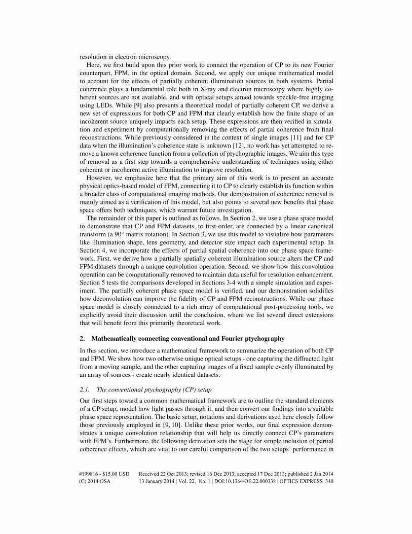
Fig. 1. Conventional ptychography’s optical setup. A sample ψ (in green) is shifted throughmany positions as the intensity of the probe light it diffracts is recorded at a far-field de-tector. In a typical visible light setup, the lens at A(r′) is a multi-element system containingthe aperture stop a(r′) at some intermediate plane, as diagrammed.

Section 5. Reciprocal space coordinates will be designated with the absence of a prime, andreciprocal space functions will include a tilde (e.g., the Fourier transform of a(r′) is a(r)). Notethat here both r and r′ will have units of meters, since they represent the spatial axis of animaging system’s two Fourier conjugate planes. A schematic diagram of a scanning CP setupcontaining two sets of such planes is in Fig. 1. While deviations exist, most recent ptycho-graphic experiments generally follow Fig. 1’s optical outline. The following analysis considersa two-dimensional imaging geometry, for simplicity. Extension to three dimensions is direct.

A standard CP setup first focuses light from an illumination plane I(r) onto a shifting sampleand records a series of far-field diffraction patterns. We assume I(r) contains an ideal point lightsource that produces a quasi-monochromatic plane wave (wavelength λ ) propagating parallelto the optical axis at a large distance `. The case of a non-ideal point source will be consideredin Section 4. At distance ` is an aperture plane A(r′) containing a lens of focal length f . Directlypast this plane, the optical field may be described across all space simply as a(r′), the aperturetransmission function.

This incident plane wave, confined to a(r′), is focused by the lens to a small area at thesample plane, S(r). Under the Fresnel approximation, the shape of the focal spot before hittingthe sample is proportional to the scaled Fourier transform of the field at aperture transmissionfunction, a(r′) [13]:

S+(r) =exp(

jk2 f r2

)jλ f

∫a(r′)exp

(− jk

fr · r′

)dr′ ≈F

[a(r′)

]= a(r), (1)

where F is the Fourier transform operator, S+(r) is the field directly before the sample, andthe approximation assumes the phase pre-factor is unity. This common unity approximation isused e.g. in [9]’s related analysis and is justified for a well-corrected Fourier-transforming lensin [13]. It becomes mathematically evident when considering typical samples much smallerthan the lens focal length, with r << f . All integrals are assumed to extend from negative topositive infinity. The above expression also ignores a constant coordinate scaling factor: a(r)should actually be written as a(r/λ f ). For clarity, we will generally neglect constant scalingfactors. Details of scaling effects may be found in Appendix A. a(r) typically takes the form ofa sinc function as in Fig. 2, but may be arbitrarily shaped. For example, several ptychographicsetups use a pinhole or alternative aperture to define the shape of a(r) close to the sampleplane [6, 7].

Independent of its specific distribution, the confined beam a(r) then interacts with a shiftedsample ψ to produce an exiting optical field, S(r). We assume the effect of sample thickness

r' (m

)!

x (m) !

Wψ (r, u)!

= *

Wa (r, u)!u

(m-1

) !

r (m)!

Data Matrix

m (x, r')!

Sample ψ(r-x )!

Plane S(r)!

xth diffraction image !

Plane D(r')!

F [ψ(r-x) a(r)]

r-x (mm)! r' (mm)!

WD

F m

odel!

optic

al fi

eld!

-.2! .2!

Probe a(r )!

PTY!

r (mm)!

Intensity (AU)!

�

Shift!

-.1! .1! -.2! .2!

u (m

-1) !

r (m)!-.2!

1!

0!

1!

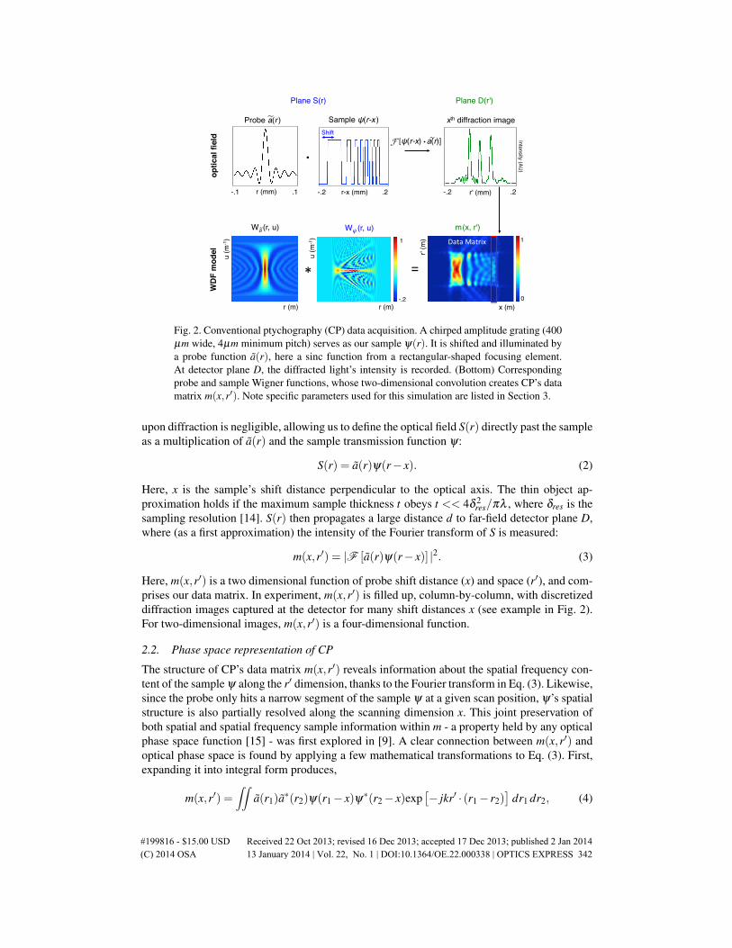
Fig. 2. Conventional ptychography (CP) data acquisition. A chirped amplitude grating (400µm wide, 4µm minimum pitch) serves as our sample ψ(r). It is shifted and illuminated bya probe function a(r), here a sinc function from a rectangular-shaped focusing element.At detector plane D, the diffracted light’s intensity is recorded. (Bottom) Correspondingprobe and sample Wigner functions, whose two-dimensional convolution creates CP’s datamatrix m(x,r′). Note specific parameters used for this simulation are listed in Section 3.

upon diffraction is negligible, allowing us to define the optical field S(r) directly past the sampleas a multiplication of a(r) and the sample transmission function ψ:

S(r) = a(r)ψ(r− x). (2)

Here, x is the sample’s shift distance perpendicular to the optical axis. The thin object ap-proximation holds if the maximum sample thickness t obeys t << 4δ 2

res/πλ , where δres is thesampling resolution [14]. S(r) then propagates a large distance d to far-field detector plane D,where (as a first approximation) the intensity of the Fourier transform of S is measured:

m(x,r′) = |F [a(r)ψ(r− x)] |2. (3)

Here, m(x,r′) is a two dimensional function of probe shift distance (x) and space (r′), and com-prises our data matrix. In experiment, m(x,r′) is filled up, column-by-column, with discretizeddiffraction images captured at the detector for many shift distances x (see example in Fig. 2).For two-dimensional images, m(x,r′) is a four-dimensional function.

2.2. Phase space representation of CP

The structure of CP’s data matrix m(x,r′) reveals information about the spatial frequency con-tent of the sample ψ along the r′ dimension, thanks to the Fourier transform in Eq. (3). Likewise,since the probe only hits a narrow segment of the sample ψ at a given scan position, ψ’s spatialstructure is also partially resolved along the scanning dimension x. This joint preservation ofboth spatial and spatial frequency sample information within m - a property held by any opticalphase space function [15] - was first explored in [9]. A clear connection between m(x,r′) andoptical phase space is found by applying a few mathematical transformations to Eq. (3). First,expanding it into integral form produces,

m(x,r′) =∫∫

a(r1)a∗(r2)ψ(r1− x)ψ∗(r2− x)exp[− jkr′ · (r1− r2)

]dr1 dr2, (4)


where the double integral over new spatial variables (r1,r2) results from measurement of inten-sity at the detector, and ∗ denotes complex conjugate. From here, straightforward manipulationsproduce an expression for the data matrix m as a convolution of two functions:

m(x,r′) =∫∫

Wψ(r− x,u)Wa(r,r′−u)dr du, (5)

where constant pre-integral multipliers are neglected for clarity. The function W applied to ψ

takes the form,Wψ(r,u) =

∫∞

−∞

ψ

(r+

y2

)ψ∗(

r− y2

)exp(− jkyu)dy (6)

and is known as the Wigner distribution function (WDF) of ψ . Equation (5) describes CP’sset of diffraction intensity images as a convolution of two functions solely related to the shapeof the sample and the probe beam, respectively (i.e., the WDF separates the sample transmis-sion function and probe beam into a linear expression). This is graphically depicted in Fig. 2.Note that while not explicitly included in this paper, the interested reader is invited to use thederivation steps in Appendix B to help create Eq. (5) from Eq. (4).

The WDF is a well-studied phase space distribution that is often used to analyze opticalimaging setups [15–17]. Like the Fourier transform, it transfers a function of one “primal”variable r into a new space. Unlike the Fourier transform, which offers a one-to-one mappingbetween the primal variable r and its conjugate u (here a mapping between space and spatialfrequency), this new space is two-dimensional. The WDF is a joint function of both the primalspatial variable r and the conjugate spatial frequency variable u. Although defined in a higher-dimensional space, Wψ maintains a one-to-one relationship with the complex function ψ (apartfrom a constant phase shift). While not always exact, it is convenient to connect the value ofW (r0,u0) to the amount of optical power at point r0 propagating in direction u0. However, whilethe WDF is real-valued it is not necessarily non-negative, which requires this interpretation tobe taken loosely.

The goal of ptychography’s many post-processing algorithms is to recover the complex sam-ple function ψ , which has a one-to-one relationship with Wψ , from its recorded dataset m. Thisgoal is computationally related to deconvolving the effect of the aperture a, described by Wa,from m(x,r′) in Eq. (5). Deconvolution is often indirectly achieved through a phase retrievalalgorithm [18]. Before proceeding, it is worth mentioning several challenging features exhib-ited by the above CP arrangement when considered in an optical microscopy context: its lowcollection efficiency of lensless detection hampers signal-to-noise, scanning of the sample re-quires mechanical motion that introduces instabilities during detection, and the large extent ofthe probe across space is challenging to accurately characterize, although several recently de-veloped algorithms now account for this [19,20]. As we show next, the recently proposed FPMtechnique in [8] also recovers a complex sample ψ via deconvolution of a high-dimensionaldataset, but is able to circumvent the above list of limitations.

2.3. Mathematical representation of Fourier ptychographic microscopy (FPM)

FPM also acquires a sequence of images that are compiled into a data matrix (here labeled mF )but does so using the unique optical setup in Fig. 3. Two primary experimental differences setFPM apart from the CP setup outlined above: an array of n LEDs now occupy the illuminationplane I(r), and the locations of the sample and aperture planes are effectively switched. Insteadof recording the diffraction pattern from a small illuminated sample region, FPM images theentire sample under illumination from different directions.

Again, we begin by assuming each LED in the array occupying the illumination plane I(r)emits a quasi-monochromatic and spatially coherent field at wavelength λ (partially coherent


Fourier Ptychography Setup!

LED Array! Sample ψ(r' )! Aperture a(r )! Detector!

w"

δx

shift illumination angle hi" !

I(r) ! S(r') ! A(r) ! D(r') !

image mF (r' )!

do" di"l

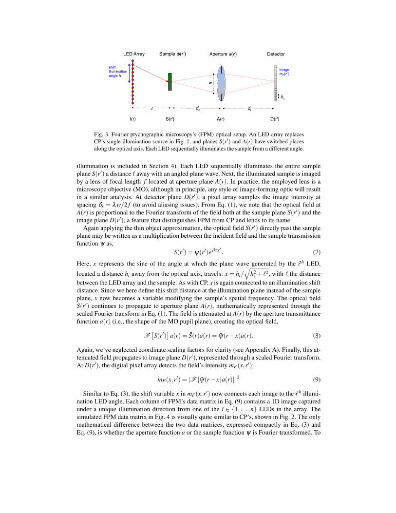
Fig. 3. Fourier ptychographic microscopy’s (FPM) optical setup. An LED array replacesCP’s single illumination source in Fig. 1, and planes S(r′) and A(r) have switched placesalong the optical axis. Each LED sequentially illuminates the sample from a different angle.

illumination is included in Section 4). Each LED sequentially illuminates the entire sampleplane S(r′) a distance ` away with an angled plane wave. Next, the illuminated sample is imagedby a lens of focal length f located at aperture plane A(r). In practice, the employed lens is amicroscope objective (MO), although in principle, any style of image-forming optic will resultin a similar analysis. At detector plane D(r′), a pixel array samples the image intensity atspacing δx = λw/2 f (to avoid aliasing issues). From Eq. (1), we note that the optical field atA(r) is proportional to the Fourier transform of the field both at the sample plane S(r′) and theimage plane D(r′), a feature that distinguishes FPM from CP and lends to its name.

Again applying the thin object approximation, the optical field S(r′) directly past the sampleplane may be written as a multiplication between the incident field and the sample transmissionfunction ψ as,

S(r′) = ψ(r′)e jkxr′ . (7)

Here, x represents the sine of the angle at which the plane wave generated by the ith LED,

located a distance hi away from the optical axis, travels: x = hi/√

h2i + `2, with ` the distance

between the LED array and the sample. As with CP, x is again connected to an illumination shiftdistance. Since we here define this shift distance at the illumination plane instead of the sampleplane, x now becomes a variable modifying the sample’s spatial frequency. The optical fieldS(r′) continues to propagate to aperture plane A(r), mathematically represented through thescaled Fourier transform in Eq. (1). The field is attenuated at A(r) by the aperture transmittancefunction a(r) (i.e., the shape of the MO pupil plane), creating the optical field,

F[S(r′)

]a(r) = S(r)a(r) = ψ(r− x)a(r). (8)

Again, we’ve neglected coordinate scaling factors for clarity (see Appendix A). Finally, this at-tenuated field propagates to image plane D(r′), represented through a scaled Fourier transform.At D(r′), the digital pixel array detects the field’s intensity mF(x,r′):

mF(x,r′) = |F [ψ(r− x)a(r)] |2 (9)

Similar to Eq. (3), the shift variable x in mF(x,r′) now connects each image to the ith illumi-nation LED angle. Each column of FPM’s data matrix in Eq. (9) contains a 1D image capturedunder a unique illumination direction from one of the i ∈ {1, . . . ,n} LEDs in the array. Thesimulated FPM data matrix in Fig. 4 is visually quite similar to CP’s, shown in Fig. 2. The onlymathematical difference between the two data matrices, expressed compactly in Eq. (3) andEq. (9), is whether the aperture function a or the sample function ψ is Fourier-transformed. To

Sample Wψ (u, r)!

= *

Data Matrix

mF (x, r' )!

Sample ψ(r' )!

Plane S(r' )!

xth low-res. image !

Plane D(r' )!

WD

F m

odel!

optic

al fi

eld!

FPM!

Aperture Wa (u, r)!

Plane A(r)!

Aperture a(r )!

amplitude! Intensity (AU)!

r (mm)! r' (mm)!-35! 35!r' (mm)!-.2! .2! -.2! .2!

r' (m

)!

x (m) !

u (m

-1) !

r (m)!

u (m

-1) !

r (m)!

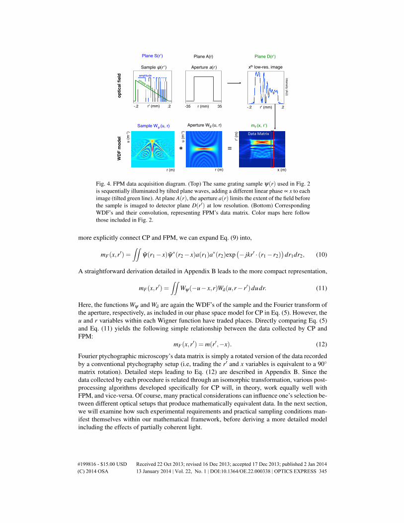
Fig. 4. FPM data acquisition diagram. (Top) The same grating sample ψ(r) used in Fig. 2is sequentially illuminated by tilted plane waves, adding a different linear phase ∝ x to eachimage (tilted green line). At plane A(r), the aperture a(r) limits the extent of the field beforethe sample is imaged to detector plane D(r′) at low resolution. (Bottom) CorrespondingWDF’s and their convolution, representing FPM’s data matrix. Color maps here followthose included in Fig. 2.

more explicitly connect CP and FPM, we can expand Eq. (9) into,

mF(x,r′) =∫∫

ψ(r1− x)ψ∗(r2− x)a(r1)a∗(r2)exp(− jkr′ · (r1− r2)

)dr1dr2, (10)

A straightforward derivation detailed in Appendix B leads to the more compact representation,

mF(x,r′) =∫∫

Wψ(−u− x,r)Wa(u,r− r′)dudr. (11)

Here, the functions Wψ and Wa are again the WDF’s of the sample and the Fourier transform ofthe aperture, respectively, as included in our phase space model for CP in Eq. (5). However, theu and r variables within each Wigner function have traded places. Directly comparing Eq. (5)and Eq. (11) yields the following simple relationship between the data collected by CP andFPM:

mF(x,r′) = m(r′,−x). (12)

Fourier ptychographic microscopy’s data matrix is simply a rotated version of the data recordedby a conventional ptychography setup (i.e, trading the r′ and x variables is equivalent to a 90◦

matrix rotation). Detailed steps leading to Eq. (12) are described in Appendix B. Since thedata collected by each procedure is related through an isomorphic transformation, various post-processing algorithms developed specifically for CP will, in theory, work equally well withFPM, and vice-versa. Of course, many practical considerations can influence one’s selection be-tween different optical setups that produce mathematically equivalent data. In the next section,we will examine how such experimental requirements and practical sampling conditions man-ifest themselves within our mathematical framework, before deriving a more detailed modelincluding the effects of partially coherent light.


r'!

x!

u!

r!

Image i

CP!

Detector width!

Pixel size!

Scan range!

Scan step!

r'!

x!

Image i

FPM!

Image FOV!

LED pitch!

Max. LED angle!

Pixel/PSF size!

Wa (r, u)!

Finite probe (overlap)!

Max. spatial frequency!

u! Wa (r, u)!

Image PSF!

(Max. scan range/accepted kx)!

r!

Dat

a m

atrix!

Blur

Ker

nel!

m (x,r') mF (x,r')

Fig. 5. The experimental factors influencing CP and FPM data matrices. (top) Geometricalfactors define the data matrix scaling and sampling, while (bottom) parameters specific tothe focusing/imaging lens define data matrix blurring for both setups.

3. Visualizing connections between both ptychographic domains

The phase space model in Section 2 offers an excellent visualization of the close link betweenthe data collected by CP and FPM. However, it is not correct to assume the exact linear rela-tionship in Eq. (12) implies that CP and FPM are always experimentally identical - a number ofsystem-specific factors may influence each data matrix uniquely. The first goal of this sectionis to use our phase space model to visualize how experimental factors impact data collection,as Fig. 5 outlines. At the same time, ensuring the two setups produce data exactly followingEq. (12)’s rotation relationship is not particularly challenging. The second goal of the follow-ing discussion is to identify a set of carefully chosen setup parameters that lead to such an exactrelationship, which we will use in Section 5’s comparison. Most experimental aspects of CPand FPM fit nicely into one of four categories describing a particular data matrix property:

1. Scaling along the optical axis: For both ptychographic procedures, distances between theoptical source, sample, detector, and the lens focal length will lead to constant scaling varia-tions along r′ and x in their respective data matrices. Details of these scaling relationships arepresented in Appendix A.

2. Sampling along r′: The digital detector’s sampling conditions for CP and FPM both mani-fest themselves along their corresponding data matrices’ r′ axis (Fig. 5, green text). For CP, thedetector width must match the aperture’s maximum transmitted spatial frequency. This widthdefines the resolution limit of a final reconstructed image. The detector size and distance to-gether define a geometric NA, which much match the detector pixel size to avoid aliasing [10].For FPM, sampling along the r′ axis follows a typical imaging setup - the detector width ispaired to the imaging lens FOV, and the detector pixel size matches the imaging optics’ point-spread function (PSF) width to avoid aliasing.

3. Scanning along x: Sampling along the data matrix x-dimension is tied to the operation ofeach setup’s illumination (Fig. 5, blue text). In CP, the probe beam’s total scanning distance setsthe maximum extent along x, which also defines the final reconstructed image’s FOV. In FPM,however, the maximum extent along x is set by the maximum LED-sample illumination angle.


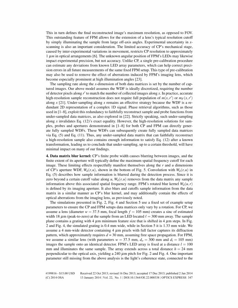
This in turn defines the final reconstructed image’s maximum resolution, as opposed to FOV.This outstanding feature of FPM allows for the extension of a lens’s typical resolution cutoffby simply illuminating the sample from large off-axis angles. Experimental uncertainty in x-scanning is also an important consideration. The limited accuracy of CP’s mechanical stage,caused by inter-experimental variations in movement, restricts CP resolution to approximately1 µm in optical arrangements [6]. The unknown angular position of FPM’s LEDs may likewiseimpact experimental precision, but not accuracy. Unlike CP, a single pre-calibration procedurecan estimate any deviations from known LED array parameters, which can help correct preci-sion errors in all future measurements of the same fixed FPM setup. This type of pre-calibrationmay also be used to remove the effect of aberrations induced by FPM’s imaging lens, whichbecome especially prominent at high illumination angles [23].

The sampling rate along the x-dimension of both data matrices is set by the number of cap-tured images. Our above model assumes the WDF is ideally discretized, requiring the numberof detector pixels along r′ to match the number of collected images along x. In practice, accuratehigh-resolution sample reconstruction does not require full population of m(x,r′) or mF(x,r′)along x [21]. Under-sampling along x remains an effective strategy because the WDF is a re-dundant 2D representation of a complex 1D signal. Phase retrieval algorithms, such as thoseused in [1–8], exploit this redundancy to faithfully reconstruct sample and probe functions fromunder-sampled data matrices, as also explored in [22]. Strictly speaking, such under-samplingalong x invalidates Eq. (12)’s exact equality. However, the high-resolution solutions for sam-ples, probes and apertures demonstrated in [1–8] for both CP and FPM can directly gener-ate fully sampled WDFs. These WDFs can subsequently create fully sampled data matricesvia Eq. (5) and Eq. (11). Thus, any under-sampled data matrix that can faithfully reconstructa high-resolution sample also contains enough information to satisfy Eq. (12) after a knowntransformation, leading us to conclude that under-sampling, up to a certain threshold, will haveminimal impact on many of our findings.

4. Data matrix blur kernel: CP’s finite probe width causes blurring between images, and thefinite extent of its aperture will typically define the maximum spatial frequency cutoff for eachimage. These limiting effects respectfully manifest themselves along the r and u dimensionsof CP’s aperture WDF, Wa(r,u), shown in the bottom of Fig. 5. Convolution with Wa(r,u) inEq. (5) describes how sample information is blurred during the detection process. Since it iszero beyond a certain cutoff value along u, Wa(r,u) removes from the data matrix any sampleinformation above this associated spatial frequency range. FPM’s rotated blur kernel Wa(u,r)is defined by its imaging aperture. It also blurs and cutoffs sample information from the datamatrix in a similar manner as CP’s blur kernel, and may additionally contain the effects ofoptical aberrations from the imaging lens, as previously noted.

The simulations presented in Fig. 2, Fig. 4 and Section 5 use a fixed set of example setupparameters to ensure the CP and FPM setups data matrices only vary by a rotation. For CP, weassume a lens (diameter w = 37.5 mm, focal length f = 105 mm) creates a sinc of estimatedwidth 18 µm (peak-to-zero) at the sample from an LED located `= 300 mm away. The sampleplane contains a grating with 4 µm minimum feature size that is shifted in 4 µm steps. In Fig.2 and Fig. 4, the simulated grating is 0.4 mm wide, while in Section 5 it is 1.33 mm wide. Weassume a 4 mm-wide detector containing 4 µm pixels with full factor captures its diffractionpattern, which approximately requires d = 30 mm, assuming free space propagation. For FPM,we assume a similar lens (with parameters w = 37.5 mm, do = 300 mm and di = 105 mm)images the sample onto an identical detector. FPM’s LED array is fixed at a distance l = 100mm and illuminates the same sample. The array extends across a total distance h = 24 mmperpendicular to the optical axis, yielding a 240 µm pitch for Fig. 2 and Fig. 4. One importantparameter still missing from the above analysis is the light’s coherence state, connected to the


active area of each optical source. We will now extend our phase space model to account forthis critical effect.

4. A complete statistical model with partially coherent light

In practice, the illumination sources used by each form of ptychography exhibit a limited spatialand temporal coherence. The rarity of ideally coherent electron and X-ray sources has led tothe theoretical and experimental examination of coherence effects in CP setups [11, 12]. Inthe next two subsections, we will primarily be interested in visible-wavelength CP setups thatmight benefit from adopting an LED illumination source. Switching to such a partially coherentsource proved a key enabling technology for FPM, as LEDs offer spatially even illuminationand can be easily arranged into inexpensive two-dimensional arrays.

Here, we use our phase space model to show that in either optical setup, partially coherentLED illumination does not limit the ability to recover an exact sample amplitude and phaseestimate. We conclude that while partial coherence impacts CP and FPM performance differ-ently, it remains a mathematical separable expression that can be removed by computationalpost-processing. Section 5 applies our model to remove known coherence blur from both CPand FPM data for the first time, and Section 6 considers future extensions to build upon thisinitial demonstration.

4.1. Partially coherent source description

To accurately model experimentally realistic optical sources, we must introduce a statisticalmeasure of spatial coherence into our phase space descriptions of CP in Eq. (5) and FPMin Eq. (11). We achieve this by treating the optical source’s emitted field U(r, t) as a tem-porally stationary stochastic process and examining its correlation across space and time:〈U(r1, t1)U∗(r2, t2)〉 = Γ(r1,r2,τ). Here, Γ is the light’s mutual coherence, τ = t2 − t1 is aconstant time difference, and the expectation value is performed over time. From the Weiner-Khinchine theorem, the cross-spectral density (CSD) of this stochastic process is defined asΓ(r1,r2,ω) =

∫Γ(r1,r2,τ)e− jωτ dτ . The spectral density C(r,ω) = Γ(r,r,ω) represents the in-

tensity of light at location r at a certain frequency ω . We will assume our illumination sourcesare fully spatially incoherent within their photon-generating area, leading to a CSD function atsource plane I,

ΓI(r1,r2,ω) = γ2C(r1,ω)δ (r1− r2), (13)

where C represents the geometric shape of the source intensity for each frequency ω (typicallya circ-function in two dimensions), γ is its spatial coherence cross section and δ is a Dirac deltafunction. For the remainder of this section, we will drop spectral dependance on ω for simplic-ity, assuming a notch filter is used in experiment to effectively isolate a narrow spectrum fromthe source. Although not detailed here, effects of a spectrally broad (i.e., temporally incoherent)source are an important consideration and may be included through incoherent superposition ofthe following equations. The Van Cittert-Zernike theorem relates Eq. (13)’s CSD of the sourceΓI in to the CSD a distance z away, Γz:

Γz(∆r′) = e− jkq

2z

∫C(r)e

jkz (r∆r′)dr ≈ C(r), (14)

where a constant multiplier is neglected for simplicity, ∆r′ = r′1−r′2 and q= r′21 −r′22 . Assuming(r′21 − r′22 )/λ z << 1 allows us to neglect the phase factor up front. With this assumption, wearrive at an approximate scaled Fourier relationship between the shape of an incoherent illumi-nation source, C, and the CSD function Γz at any subsequent plane a large distance z from thissource.


4.2. CP with partially coherent light

In conventional ptychography, the first distant plane the source’s light interacts with is theaperture plane A(r′). Here, the light’s CSD function Γ`(r′1−r′2) is given by Eq. (14), with z = `.The aperture a(r′) then modulates Γ`(r′1− r′2) before the light is focused by the lens to thesample plane, mathematically expressed by applying a Fourier transform kernel to each spatialcoordinate r′1 and r′2. Multiplying Γ`(r′1− r′2) in Eq. (14) with aperture function a and Fouriertransforming the result leads to an input-output (i.e., source-to-sample plane) CSD relationshipdefined by a convolution [24]:

ΓaS(r1,r2) =

∫C(p)a(r1− p) a∗ (r2− p)d p, (15)

where ΓaS is the CSD illuminating the sample plane S and we have used the coordinate variable

replacement p = r′ for notational clarity. We have omitted a constant scaling of p by 1/λ` andr1 and r2 by 1/λ f , for simplicity. With Eq. (15), we now have a full statistical description ofCP’s focused probe beam illuminating the sample. Our previous representation of the focusedprobe beam as a fully coherent field, simply described by a(r), is no longer valid now thatthe source has finite spatial extent. We can update our original expression for the intensity atthe detector m(x,r′) in Eq. (4) to reflect our new partially coherent probe beam with a simplereplacement. Instead of multiplying the sample ψ with coherent probe wave a, we multiply ψ

with the probe wave CSD in Eq. (15):

m(x,r′) =∫∫

ΓaS(r1,r2)ψ(r1− x)ψ∗(r2− x)exp

[− jkr′ · (r1− r2)

]dr1 dr2. (16)

Plugging Eq. (15) into Eq. (16) and performing several straightforward manipulations (outlinedin Appendix C) produces the following mathematical description of the CP data matrix m(r′,x)in terms of the aperture’s WDF, the sample’s WDF, and the illumination source’s geometricshape C:

m(x,r′) =∫∫∫

C(p)Wψ(r− x,u)Wa(r− p,r′−u)dr dud p, (17)

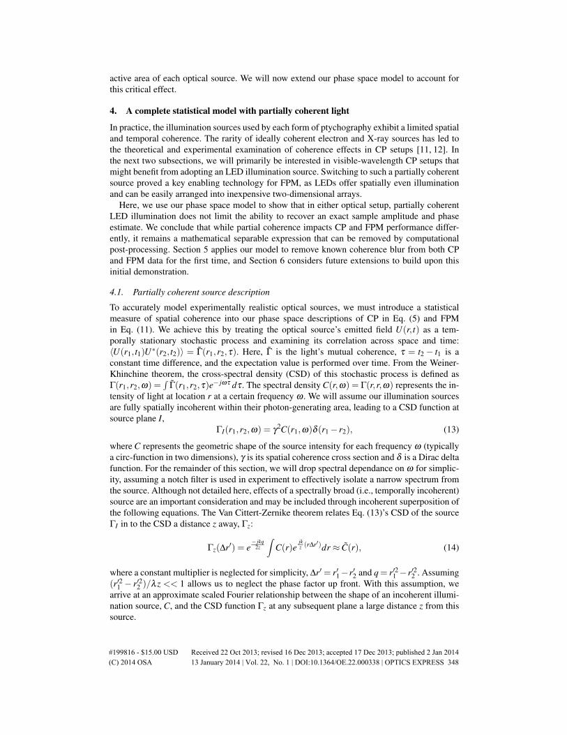
Partially coherent light alters CP’s data matrix with an additional convolution along the scanvariable x (Fig. 6(a)). The goal of ptychographic data post-processing under partially coherentillumination is to recover a complex description of the sample Wψ from data matrix m(x,r′) bydeconvolving the effects of both Wa and C. This is identical to the coherent case, but with anadditional (yet still separable) blurring term.

4.3. FPM with partially coherent light

Unlike CP, FPM uses an array of spatially offset and partially coherent LEDs at its illuminationplane. Using x to represent the distance from a given LED to the optical axis, the CSD of oneLED may be expressed by modifying Eq. (13) to incorporate a spatial offset by x: ΓI(r1,r2) =γ2C(r1 − x)δ (r1 − r2). This LED’s shifted source light first illuminates the sample at planeS(r′). Again neglecting its quadratic phase and constant scaling terms for simplicity, Eq. (14)can propagate ΓI(r1,r2) to the sample plane S(r′) to express the CSD at the sample, ΓS:

ΓS(ρ1−ρ2) =∫

C(r− x)e jkr(ρ1−ρ2)dr = C(ρ1−ρ2)exp(− jkx(ρ1−ρ2)), (18)

where (ρ1,ρ2) have replaced (r′1,r′2) as the sample’s spatial coordinates at S(r′), for notational

clarity. This illumination light is then modulated (i.e., multiplied) by the sample transmissionfunction ψ and subsequently imaged onto the detector plane. As in the previous subsection,


C(x)!

x!*

r'!

x!

=

m0 (x, r')

C(x)!

x!

(a) Conventional ptychography !

(b) FPM!

r'!

x!

m (x, r')

*

mF0 (x, r') r'!

x!

r'!

x!

=

mF (x, r')

x!

x!

blur!

blur!

0!

1!

Fig. 6. Partially coherent light manifests itself as an additional convolution along the datamatrix scan dimension x for both (a) CP and (b) FPM. The convolution is one-dimensional,as indicated by the vertical bar. With matrices rotated by 90◦ with respect to one another,this convolution will mix the data from each respective setup in a unique manner. For thissimulation, we used the same setup parameters as for Fig. 2 and Fig. 4, but assumed eachillumination source C(x) (i.e., LED) is a rectangle 200 µm in diameter.

the transformation of the CSD from the sample to the detector plane is given by a convolutionof each spatial variable ρ1 and ρ2 with a coherent impulse response [24], here defined by theFourier transform of the aperture a:

ΓD(r′1,r′2) =

∫∫ΓS(ρ1−ρ2)ψ(ρ1)ψ

∗(ρ2)a(ρ1− r′1)a∗(ρ2− r′2)dρ1 dρ2. (19)

ΓD(r′1,r′2) is the CSD of partially coherent light at the detector. The imaging system’s coherent

impulse response a is typically a scaled sinc function. The measured intensity at the detectoris given by evaluating ΓD at one spatial location r′ = r′1 = r′2. This allows us to express FPM’smeasured data as mF(x,r′) = ΓD(r′,r′), where mF(x,r′) is the same data matrix from Section 3.By substituting Eq. (18) into Eq. (19) and setting r′1 = r′2 = r′ we obtain the following expressionfor the recorded image intensity mF(x,r′) as a function of LED offset x and detector positionr′:

mF(x,r′) =∫∫

C(ρ1−ρ2)ψ(ρ1)ψ∗(ρ2)a(ρ1− r′)a∗(ρ2− r′)exp(− jkx(ρ1−ρ2)) dρ1 dρ2.

(20)Equation (20) resembles our coherent FPM data matrix expression in Eq. (10), but now with anadditional C term accounting for partial coherence effects. As detailed in Appendix D, Eq. (20)may be rearranged into a final expression in terms of the aperture WDF, sample WDF, and LEDsource geometry:

mF(x,r′) =∫∫∫

C(p)Wψ(p−u− x,r)Wa(u,r− r′)dr dud p. (21)

Comparing Eq. (21) to Eq. (11)’s coherent description of FPM, we see that partial coherencemanifests itself as an additional convolution along the data matrix x-dimension (Fig. 6(b)). Prac-tically, this indicates each FPM image, captured from a different LED and compiled along x,


will begin to look increasingly similar with increasingly incoherent illumination. In the limit ofa completely incoherent source, spatial shifting will leave all image features nearly unchanged.Since this blur remains a separable function, it is still possible to deconvolve the effects of bothC and Wa to obtain an accurate sample estimate Wψ . Comparing Eq. (21) to Eq. (17)’s expres-sion for partially coherent CP, we find a new primary difference between the two setups: whilepartial coherence alters both data matrices along the x dimension (the scan variable), it changesthe underlying structure of each data matrix differently, since each is rotated by 90◦ with re-spect to the other. Put simply, using a partially coherent source in a CP setup blurs together thesample’s spatial information within its recorded data matrix. In FPM, using an array of partiallycoherent sources blurs the sample’s spatial frequency content, as Fig. 6 clearly depicts.

5. Case study: CP and FPM under partially coherent illumination

To briefly demonstrate the validity of our phase space model, we now attempt to measure and re-move the effects of partial coherence in example CP and FPM data matrices, both in simulationand experiment. This exercise allows us to check the accuracy of our final statistical descrip-tions in Eq. (17) and Eq. (21). In addition, this demonstration also offers the following threeprimary insights. First, FPM setups that currently rely upon partially coherent LED arrays mayimprove the fidelity of their reconstructions by adopting this coherence removal procedure, asour tests establish. Second, the only currently demonstrated procedure that accounts for partialcoherence within CP data does so without knowledge of the illumination coherence function,C(p) [12]. The proposed coherence removal algorithm takes into account a-priori knowledge ofC(p), offering a more robust procedure when an estimate of the illumination source’s shape isavailable. Third, our experiment tracks the slow degradation of phase imaging performance asa function of decreasing source coherence. To the best of our knowledge, it is still not currentlywell-understood why phase acquisition is possible yet noisy with low-coherence illumination,and our findings may generalize to benefit this area of investigation.

For both simulation and experiment, we carefully designed the scaling and distance param-eters to match those listed at the end of Section 3 for three purposes. First, these optimizedparameters ensure both data matrices m and mF match, after a rotation. Second, the listed pa-rameters require both setups to use the same lens numerical aperture, detector pixel size andcount, and nearly the same total optical path length, offering as even a comparison as possible.Third, the parameters correspond closely with previous optical CP [6, 7] and FPM [8] experi-mental testing platforms. One exception to this close match is the width of the CP’s probe beamat the sample plane, which is typically allowed to be several times wider than what we simulateto allow for under-sampling along x by a similar factor.

5.1. Simulation

In our first investigation, we simulate the partially coherent imaging performance of CP andFPM as a function of LED size. Both systems capture 350 one-dimensional images containing103 pixels each, which combine to form each data matrix. Note that all figures display thecentral 350-pixel area of each captured image to aid in visualization. As in Fig. 2 and Fig.4, our sample here is a chirped grating with minimum feature size of 4 µm. Unlike previoussimulations, the grating is now 1.33 mm-wide and is of a slightly different structure to match ourexperimental sample (see Fig. 7(d)). We first apply a Fresnel-based propagation simulation tocreate this grating’s CP and FPM data matrices under partially coherent illumination, as in Fig.7(a)-(b). We then numerically compute Eq. (17) and Eq. (21) using the same grating functionψ (including all relevant scaling factors in Appendix A). In doing so, we find agreement up toan average error of < 1% caused by numerical approximation, which verifies our phase spaceformulation.


r'!

x!

(a) CP!

(b) FPM!

m (x, r')

r'!

x!

W-1(C, σ)!

r'!

x!

RMSEp = 0.065

r'!

x!

RMSEF = 0.029

W-1(C, σ)!

mF (x, r')

Blurred: C = 100μm ! Deconvolved!(c) Ptychography and FPM recovery error vs. LED size!

ψ (r )!

r' (mm)!-.7! .7!

(d) Input data m0(x, r')!

r'!

x!0!

1!

Fig. 7. Simulation of partially coherent effects produce blurred (a) CP and (b) FPM datamatrices of an example grating. A Wiener filter can approximately recover the coherentdata matrix for each setup, from which an accurate sample reconstruction is direct. (c)Reconstruction error as a function of LED diameter (i.e., blur kernel width) increases forboth CP and FPM, although FPM’s error is consistently lower. (d) The chirped gratingsample and its coherent CP data matrix, for comparison.

Given a valid model, we next test if partial coherence effects can be effectively removed fromCP and FPM. Successful digital removal of the blurring effects caused by a finite source shapeC will allow both setups to maintain high-resolution imaging performance using larger, brighteroptical sources (i.e., with higher photon throughput). As a standard benchmark, we apply thewell-known Wiener filter in our deconvolution attempt. Previously used to recover complexsample data in [9, 10], it has since been replaced by more advanced phase retrieval-based algo-rithms [12, 18, 19]. However, since the Wiener filter offers mean-squared error (MSE) optimalfiltering performance for a stationary signal [25], it is well-suited for our simple demonstration.

The example blurred CP and FPM data matrix inputs in the left of Fig. 7(a)-(b) assumequasi-monochromatic illumination from sources with 100 µm-diameter active area (0.11◦ an-gular extent). The associated Wiener deconvolution outputs are shown directly to the right.Gaussian noise (normalized variance of 10−3) was added to the data before deconvolution.Noise variance and source size were assumed as prior knowledge to assure optimal filter per-formance. Figure 7(c) plots the average root-mean-squared error (RMSE) of recovered datamatrices as a function of source diameter after Wiener deconvolution. Each point in this plot isan average over 10 experiments with noise variances ranging evenly from 10−2 to 10−4. Thelinear process of recovering a sample estimate from its coherent data matrix ensures samplereconstruction RMSE will follow a similar curve. CP and FPM setups that do not create a fullysampled data matrix (i.e., that under-sample along x) still benefit from a similar deconvolutionapproach. While beyond the scope of this work, we have successfully applied a blind decon-volution algorithm to under-sampled CP and FPM data matrices to achieve nearly equivalentcoherence removal performance.

Two important trends are worth noting. First, RMSE increases as a function of LED diameter,but accurate sample recovery is still possible up to quite large-diameter sources. In the testedsetup, an angular source extending up to a 0.5◦ maintained manageable error after deconvolu-tion (under realistic noise assumptions). Second, it is easier to globally remove the effects of


(a) S

imul

atio

n!(b

) Exp

erim

ent!

C = 150 μm! C = 250 μm! C = 1000 μm!

x (mm)!

r' (m

m)!

2.5!0!0!

1.5!

r' (m

m)!

0!

1.5!

0!

1!

Intensity (AU)!

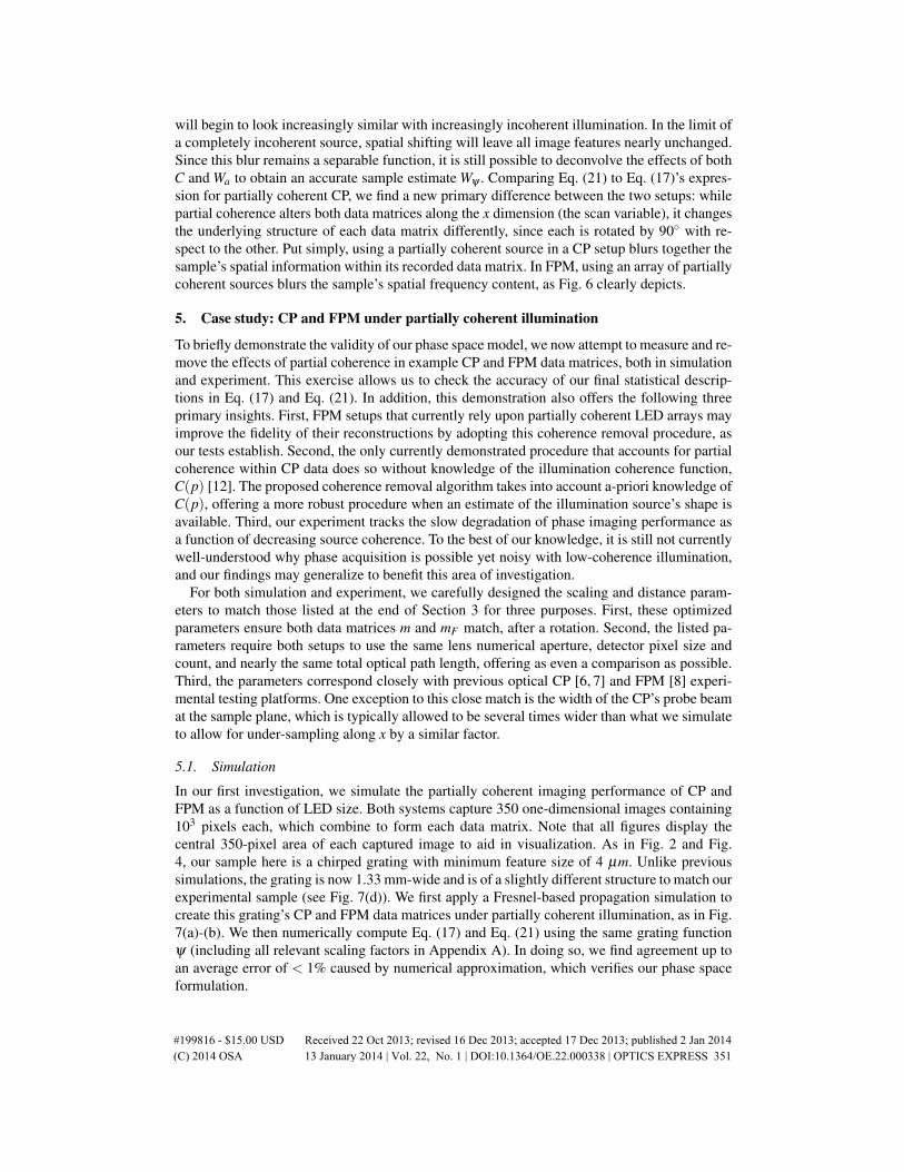
Fig. 8. (a) Simulated and (b) experimental FPM data matrices with varying degrees of par-tially coherent illumination. The experimental sample closely matches the distribution ofψ(r) in Fig. 7(d). C at top indicates the LED active area diameter used in each experiment.

partial coherence from FPM’s data matrix than from CP’s. This key conclusion is a result of thedirection of features within the data matrix for this particular simulated object. Blurring occursalong the chirped grating ridges for FPM, while it blurs the ridges together for CP, which isharder to invert. Since we expect intensities will vary more quickly along a biological sample’sspatial dimension as opposed to its spatial frequency, the trend of superior FPM performanceshould hold for most samples of interest (biological samples tend towards sparse spatial dis-tributions).

5.2. Experiment

To experimentally verify the findings of the simulation in Fig. 7, we constructed a simplifiedFPM setup with an illumination system to scan along one dimension. Experimental parametersclosely match the parameters used in simulation (see Section 3). Our experimental setup ex-hibits two primary differences from the diagram in Fig. 3. First, a single LED on a motorizedlinear stage (Newport ESP301) was used instead of a fixed LED array at illumination plane Ito facilitate easy variation of LED coherence area. This variation was achieved by placing pin-holes of different diameter (100 µm-1000 µm) directly in front of the active area of a 532 nmcentral-wavelength diode. Note that while sufficient for the current experiment, a mechanicalstage setup offers resolutions that are generally inferior to LED array-based FPM, since me-chanical motion introduces the same inaccuracies limiting CP’s achievable resolution. Second,an f = 50 mm, w = 50 mm collection lens was inserted 50 mm in front of the LED source toassure uniform illumination of the sample. We experimentally determined this lens has mini-mal effect on the coherence area at the detector plane. Our imaging setup used a f = 105 mm,w = 37.5 mm compound lens (Nikon Micro-Nikkor f/2.8G) positioned do = 300 mm from thesample that imaged onto a 4.54µm pixel CMOS array (Prosilica-GX 1920).

Figure 8 displays an example set of simulated and experimental data matrices of the samechirped grating sample in Fig. 7 under three different illumination coherence states. Each datamatrix was compiled by scanning the LED-pinhole unit at 250µm steps across 25 mm, for atotal of 100 samples along x. This sampling rate is approximately 4-5 times higher than priordemonstrations of FPM [8,26], which is not significant enough to alter any of our experimentalconclusions. At each step along x, we capture an image of the linear grating and select a singlerow of the CMOS detector array to form data matrix column x. Each image’s maximum pixelvalue is scaled to 1 (i.e., each data matrix column in Fig. 8 is normalized to it’s maximum value),


which enhances the appearance of noise in low-intensity areas but aids with visualization ofcoherence effects. The wiggling effect observable within the experimental data matrix (i.e.,shifting of the grating image as a function of illumination angle) has two primary causes. First,shifting at the image plane may occur for samples not in ideal focus, which our detector’sslight undersampling prevents an exact verification of. Second, the grating’s finite thickness (3mm) does not accurately match the thin object approximation from Section 2, leading to anunaccounted for phase modification that manifests itself as this irregular artifact.

Figure 8 highlights three important effects of illumination coherence on FPM’s data. First, thestriped “diffraction cone” within each matrix mF(x,r′) broadens along the x-dimension whenusing a larger-diameter source, as the convolution relationship in Eq. (21) predicts. Conceptu-ally, an increasingly incoherent source will extend the lens’s coherent spatial frequency cutoffat k·NA to its incoherent spatial frequency cutoff at 2k·NA, hence broadening what is capturedalong x. This slight improvement in spatial resolution is also present (although difficult to dis-cern) within each individual image along the r′-dimension. Second, Eq. (21)’s convolution alsopredicts features along x to blur with increased incoherence, which is clearly observed at theedge of the diffraction cone. As just noted, this blurring does not impact the spatial resolution ofeach image, but instead causes images captured by adjacent LEDs to become increasingly sim-ilar, and thus harder to accurately extract sample phase from. Finally, incoherent illuminationstill allows the FPM setup to acquire high-frequency sample information that otherwise wouldnot be captured by a conventional imaging setup. This is indicated by the dark “tails” at the bot-tom of each data matrix, which represent high-frequency grating information that is diffractedinto the imaging lens from an off-axis LED, otherwise cutoff from a single image. The densityof this high-frequency information tail decreases with increasingly incoherent illumination.However, it is still clearly present with a low-coherence source, thus allowing computationalimprovement of a reconstructed image’s resolution beyond the conventional imaging lens NAcutoff. This information-preserving feature of ptychography in the presence of incoherent lightis a very powerful tool that has yet to be studied in full, and is the main conclusion of thisexperiment.

6. Conclusion and future work

To briefly summarize, we first derived a linear relationship connecting the data matrices cap-tured by conventional and Fourier ptychography. We then demonstrated that partial coherencealters different features of each setup’s data matrix, although effectively blurring both. Simula-tion and experiment verified the successful removal of such partial coherence artifacts for bothsetups, although removal from FPM’s data set is expected to yield lower error for most sparsebiological samples of interest. Besides this ancillary benefit, the FPM setup requires no movingcomponents, which thus suggests it may be capable of greater stability with respect to CP.

In the future, our derived phase space model may help advance ptychography’s developmentwith several useful hardware modifications. First, following concepts well-known in linear filterdesign, the convolution relationships in Eq. (17) and Eq. (21) indicate that careful modificationof each data matrix blur kernel can greatly reduce sample recovery error. CP’s conventional sincprobe and FPM’s typical circular aperture both include many transfer function zeros, which arecomputationally impossible to invert. Apodization of the probe and aperture with a designedmask can improve this inversion, offering increased solution stability, independent of recoveryalgorithm specifics. Apodization of the incoherent illumination source’s finite shape, C(p), willalso improve removal of partial coherence effects. Second, Eq. (12) suggests that alternative op-tical setups can capture the data matrix m under different linear transformations (e.g., a matrixrotation that is not 90◦, or another isomorphic transform besides rotation). These alternativesto CP and FPM will most likely offer application-specific advantages. For example, one could


imagine both shifting the sample across a limited range and using a small number of illumi-nation sources to increase collection efficiency. This specific joint CP-FPM setup may benefitapplications only tolerating minimal movement, but many other hybrid designs may be easilyimagined to fulfill niche design constraints. Finally, we minimally considered the computa-tional post-processing aspect of ptychography in our analysis. As recently demonstrated, phasespace offers a rich array of image reconstruction tools [22]. Working within a high-dimensionalspace like the WDF’s is required when including partial coherence, so our model will mostimmediately impact ptychographic algorithms that must account for the effects of large, high-throughput sources. Furthermore, our demonstration of a linear mapping between CP and FPMassures that any future computational developments may jointly benefit both setups. For ex-ample, we now know FPM can immediately benefit from recent CP algorithms like ePIE [19],annealing [20], and other procedures accounting for partial coherence [12]. Such sharing be-tween two previously disconnected research areas is the most immediate impact our phase spacemodel, which we believe offers a solid foundation for many future insights to expand upon asptychography continues to evolve.

Appendix A: Phase space expressions with scaling factors included

Re-working CP’s data matrix to include coordinate scaling reveals two primary effects. First,propagation from the lens to the sample includes a λ f scaling factor [13], where λ is wave-length and f the lens focal length. Second, propagation from the sample to the detector includesa similar scaling factor by λd, with d the detector distance. A scaled version of Eq. (3) is thus,

m(x,r′) = |Fr,r′/λd [a(r/λ f )ψ(r− x)] |2, (22)

where the subscripts indicate the original and transformed coordinates used within the Fouriertransform exponent. This can be rewritten in integral form as,

m(x,r′) =∫∫

a(

r1

λ f

)a∗(

r2

λ f

)ψ(r1− x)ψ∗(r2− x)exp

[− jk

dr′ · (r1− r2)

]dr1 dr2 (23)

From here, a scaled Wigner convolution relationship is found as,

m(x,r′) =∫∫

Wψλ f

(r− x

λ f,u)

Wa

(r,

λ fd

r′−u)

dr du. (24)

where the ψλ f subscript indicates the coordinate system of Wψ is multiplicatively scaled by aconstant λ f factor. Pre-integral multiplicative constants are omitted for clarity. Equation (24)includes three primary effects of scaling. First is the λ f scaling factor along Wψ ’s spatial vari-able r, which also necessarily requires the phase space function’s spatial frequency variable u tobe contracted by the same proportion before computing the convolution. Second, the resultingdata matrix’s r′ coordinate is scaled by a λ f/d factor, and third its x coordinate by 1/λ f .

Scaling effects can similarly be incorporated into FPM’s data matrix Eq. (10) as,

mF(x,r′) =∫∫

ψ

(r1

λdo− x

λ

)ψ∗(

r2

λdo− x

λ

)a(r1)a∗(r2)exp

(− jkr′

λdi· (r1− r2)

)dr1dr2.

(25)Here, do is the distance from the sample to the lens and di is the distance from the lens to thedetector (Fig. 3). Straightforward manipulations following Appendix B’s steps lead to,

mF(x,r′) =∫∫

Wψλdo(−u−dox,r)Wa

(u,r− λdor′

di

)dudr. (26)


where ψλdo here indicates Wψ is fully scaled by a constant factor 1/λdo. Again, three maindifferences are apparent comparing the above to the FPM convolution expression in Eq. (11):r′ is scaled by λdo/di, x is scaled by do, and Wψ ’s joint coordinates are scaled by 1/λdo beforeconvolution. Similar manipulations yield scaling factors for data matrices containing the effectsof partially coherent illumination.

Appendix B: The Wigner representation of the FPM data matrix

Our goal in this derivation is to transform Eq. (10) into an expression separable in ψ and a,for direct comparison with Eq. (5). This can be achieved by taking advantage of the Wignerdistribution function (WDF). As noted in Section 2, the WDF is a convenient tool to achievevariable separation. The WDFs describing ψ and a are obtained by first transforming (r1, r2) tocenter-difference coordinates (r,y), using r1 = r+ y/2 and r2 = r− y/2:

mF(x,r′) =∫∫

ψ

(r+

y2− x)

ψ∗(

r− y2− x)

a(

r+y2

)a∗(

r− y2

)× exp

(− jkr′ · y

)dydr,

(27)

where in the exponent we use the fact that r1− r2 = y. Following the definition of the WDF inEq. (6), we can define the WDF of the Fourier transform of our sample function ψ as,

Wψ(r,u) =∫

ψ

(r+

y2

)ψ∗(

r− y2

)exp(− jkyu)dy. (28)

Applying an inverse Fourier transform to both sides of Eq. (28) yields,

ψ

(r+

y2

)ψ∗(

r− y2

)=

k2π

∫Wψ(r,u)exp( jkyu)du (29)

The Wigner distribution of the aperture function a(r), Wa(r,u), will take a similar form asEq. (28). As we will see next, it is more useful to express the WDF of the aperture with ashifted spatial frequency term, Wa(r,r′−u):

Wa(r,r′−u) =∫

a(

r+y2

)a∗(

r− y2

)exp(− jky(r′−u)

)dy (30)

The inverse Fourier transform of Eq. (30) yields,

a(

r+y2

)a∗(

r− y2

)=

k2π

∫Wa(r,r′−u)exp

(jky(r′−u)

)d(r′−u) (31)

Inserting Eq. (29) and Eq. (31) into Eq. (27) and noting all terms in the exponent cancel pro-duces a near-final FPM data matrix expression:

mF(x,r′) =∫∫

Wψ(r− x,u)Wa(r,r′−u)dr du, (32)

where the pre-integral multiplier is omitted for clarity. To fully connect FPM’s data matrix withCP’s in Eq. (5), we can take advantage of a convenient property of the Wigner distribution. Asa function of both space and spatial frequency, it is clear that Wψ(r,u) must contain the sameinformation as when it is applied to the sample’s Fourier transform, Wψ(r,u). The two Wignerfunctions are connected by,

Wψ(r,u) =Wψ(−u,r). (33)

The Wigner distribution of the sample’s Fourier transform ψ is given by the Wigner distributionof the sample ψ in Eq. (28) but rotated 90◦ [15]. Applying this property to both WDFs in


Eq. (32), without swapping the dummy convolution variables, produces an expression directlycomparable with CP’s Eq. (5):

mF(x,r′) =∫∫

Wψ(−u− x,r)Wa(u,r− r′)dudr, (34)

which is in Eq. (11). Two manipulations applied to Eq. (34) lead to the 90◦ rotation relationshipbetween the CP and FPM data matrices in Eq. (12). First, both the data matrix on the left ofEq. (34) and the two Wigner functions on the right of Eq. (34) must be rotated by swappingthe order of their variables (i.e., mF(x,r′) becomes mF(r′,x)). Second, the dummy integrationvariables x and r′ must switch from one Wigner function to the other (i.e., x goes to Wa and r′

goes to Wψ ). Comparing the result of these operations with Eq. (5) leads to Eq. (12)’s lineartransform.

Appendix C: Conventional ptychography with partially coherent source, derivation

The influence of partially coherent light on conventional ptychography is derived by first in-serting the CSD function of light at the sample plane (Eq. (15)) into our data matrix m(x,r′) inEq. (16) to produce,

m(x,r′) =∫∫∫

C(p)a(r1− p) a∗ (r2− p)ψ(r1− x)ψ∗(r2− x)

× exp[− jkr′ · (r1− r2)

]dr1 dr2 d p.

(35)

Next, we perform the variable substitution r1 = r+ y/2 and r2 = r− y/2 to create,

m(x,r′) =∫∫∫

C(p)a(

r+y2− p)

a∗(

r− y2− p)

ψ

(r+

y2− x)

ψ∗(

r− y2− x)

× exp[− jkr′y

]dydr d p.

(36)

Following the same steps as Eq. (28) - Eq. (29), we may replace the ψ(r+ y

2 − x)

ψ∗(r− y

2 − x)

term with its WDF to yield,

m(x,r′) =k

2π

∫∫∫∫C(p)a

(r+

y2− p)

a∗(

r− y2− p)

Wψ(r− x,u)

× exp[

jky · (u− r′)]

dydr d pdu(37)

Likewise, a similar WDF relationship may be constructed for the aperture:

a(

r+y2− p)

a∗(

r− y2− p)=

k2π

∫Wa(r− p,r′−u)exp

(jky(r′−u)

)d(r′−u) (38)

Inserting Eq. (38) into Eq. (37) and neglecting constant multipliers leads to,

m(x,r′) =∫∫∫∫

C(p)Wa(r− p,r′−u)Wψ(r− x,u)

× exp(

jky(u− r′+ r′−u))

dydr d pdud(r′−u).(39)

Noting all terms in the exponent cancel and the dy and d(−r′−u) integrals drop to leave,

m(x,r′) =∫∫∫

C(p)Wa(r− p,r′−u)Wψ(r− x,u)dr dud p, (40)

the final expression in Eq. (17). The finite extent of the incoherent source C(p) alters our orig-inal expression for CP’s data matrix through a convolution along the x-dimension of the datamatrix, similar to FPM as derived in Appendix D.


Appendix D: FPM with partially coherent sources, derivation

Here, we would like to express Eq. (20) as a convolution between three unique functions rep-resenting the source, sample and aperture, respectively. Separating their effects will allow fordirection comparison with the partially coherent CP expression in Eq. (17), and will also helpus understand how partial coherence alters FPM’s data matrix. First, inserting the Fourier trans-form integral C(ρ1−ρ2) =

∫C(p)exp(− jkp(ρ1−ρ2)) d p into Eq. (20) leads to,

mF(r′,x) =∫∫∫

C(p)ψ(ρ1)ψ∗(ρ2)a(ρ1− r′)a∗(ρ2− r′)

× exp(− jk(x+ p)(ρ1−ρ2)) dρ1 dρ2 d p.(41)

Then, we can make a variable substitution t = x+ p to create,

mF(r′,x) =∫∫∫

C(t− x)ψ(ρ1)ψ∗(ρ2)a(ρ1− r′)a∗(ρ2− r′)

× exp(− jkt(ρ1−ρ2)) dρ1 dρ2 dt(42)

As above, we first make the variable substitution ρ1 = r+ y/2 and ρ2 = r− y/2:

mF(r′,x) =∫∫∫

C(t− x)ψ(

r+y2

)ψ∗(

r− y2

)a(

r+y2− r′)

a∗(

r− y2− r′)

× exp(− jkty) dr dydt,(43)

Then, substituting the following Wigner distributions,

a(

r+y2− r′)

a∗(

r− y2− r′)=

k2π

∫Wa(r− r′,u)exp( jkyu) du (44)

ψ

(r+

y2

)ψ∗(

r− y2

)=

k2π

∫Wψ(r, t−u)exp( jky(t−u)) d(t−u) (45)

into our expression for intensity at the detector and noting all exponential terms cancel (similarto what is shown in Eq. (39)) yields,

mF(r′,x) =∫∫∫

C(t− x)Wψ(r, t−u)Wa(r− r′,u)dr dt du. (46)

To convert this into a form directly comparable to both CP and FPM under coherent illumina-tion, we first remove t from Eq. (46) using the relationship t− x = p. Second, we note that theposition of the x and r′ variables are along opposite dimensions of Wψ and Wa as compared withour previous data matrix expression in Eq. (11). Swapping the order of variables on both sidesof Eq. (46) produces,

mF(x,r′) =∫∫∫

C(p)Wψ(x+ p−u,r)Wa(u,r− r′)dudr d p, (47)

which is directly comparable to Eq. (11). Now, partial coherence effects are included with a con-volution with source shape C along the data matrix x dimension. Comparing the above equationto Eq. (17) reveals that although C blurs both data matrices along x, the WDFs describing eachare rotated by 90◦ with respect to the other, leading partial coherence to mix together the datacaptured by CP and FPM in a different fashion.

Acknowledgments

The authors acknowledge funding support from the National Institutes of Health (grant no.1DP2OD007307-01) and Clearbridge Biophotonics Pte Ltd., Singapore (Agency Award no.Clearbridge 1). The authors would like to thank Mark Harfouche, Benjamin Judkewitz andXiaoze Ou for helpful feedback during manuscript preparation.


A phase space model of Fourier ptychographic...

Documents

Transcript of A phase space model of Fourier ptychographic...