A numerical study of channelling in heterogeneous versus ...

SVENSK KÄRNBRÄNSLEHANTERING AB

SWEDISH NUCLEAR FUEL

AND WASTE MANAGEMENT CO

Box 3091, SE-169 03 Solna

Phone +46 8 459 84 00

skb.se

SVENSK KÄRNBRÄNSLEHANTERING

A numerical study of channelling in heterogeneous versus calibrated homogenous discrete fracture network realisations

Tomas Bym

Sven Follin

Report

R-19-24May 2020

Updated 2020-10

A numerical study of channelling in heterogeneous versus calibrated homogeneous discrete fracture network realisations

Tomas Bym, Sven Follin Golder Associates AB

ISSN 1402-3091SKB R-19-24ID 1867762

May 2020

Keywords: Channelling, Discrete Fracture Network (DFN), Flow modelling

This report concerns a study which was conducted for Svensk Kärnbränslehantering AB (SKB). The conclusions and viewpoints presented in the report are those of the authors. SKB may draw modified conclusions, based on additional literature sources and/or expert opinions.

A pdf version of this document can be downloaded from www.skb.se.

© 2020 Svensk Kärnbränslehantering AB

The original report, dated May 2020, was found to contain editorial errors which have been corrected in this updated version.

SKB R-19-24 3

Abstract

The aim of this study is to evaluate if a flow-calibrated DFN model, where each fracture is hydrauli-cally homogenous, can reproduce the particle tracking behaviour of a synthetic DFN model where each fracture is hydraulically heterogeneous. The study is divided into three steps. First, steady-state pumping tests are simulated using several realisations generated with the heterogeneous DFN model. Second, recollecting the fracture geometries of these realisations, PEST® is used for flow-cali bra tion of a DFN model where each fracture is assumed hydraulically homogenous. Finally, particle tracking is conducted for all DFN realisations. The particle pathways are statistically analysed in terms of particle travelled distance, travel time and F-factor. Although PEST® is able to successfully calibrate the homogenous DFN realisations so that the distributions of pumping test results match those of the heterogeneous DFN realisations, the results demonstrate that homogeneous DFN realisations could still give poor match regarding particle transport properties.

4 SKB R-19-24

Sammanfattning

Syftet med denna studie är att utvärdera om en flödeskalibrerad DFN-modell med hydrauliskt homo-gena sprickor kan reproducera partikelspårningsbeteendet hos en syntetisk DFN-modell där sprick-orna är hydrauliskt heterogena. Studien är indelad i tre steg. I det första steget simuleras stationära pumptester för flera realiseringar genererade med den heterogena DFN-modellen. I det andra steget används PEST® för flödeskalibrering av en DFN-modell där de heterogena sprickornas geometrier är oförändrade men de hydrauliska egenskaperna antas vara homogena. Slutligen genomförs partikel-spårning för samtliga DFN realiseringar. Partikelvägarnas egenskaper analyseras statistiskt med avseende på längd, gångtid och flödesrelaterat transportmotstånd (F-faktor). Även om PEST® är i stånd att kalibrera de homogena DFN realiseringarna så att fördelningarna av pumptestresultaten matchar de som erhålls med de heterogena DFN realiseringarna, visar resultaten att homogena DFN realiseringar fortfarande kan ge dålig matchning beträffande partikeltransportegenskaper.

SKB R-19-24 5

Contents

1 Introduction 71.1 Background 71.2 Objectives 71.3 Workflow 71.4 Report structure 8

2 Technical developments and software 92.1 Heterogeneous fracture properties 92.2 Particle tracking 102.3 Histogram comparison 112.4 Commercial and/or open-source software 12

2.4.1 FracMan®, MeshMaster® and Mafic® 122.4.2 PEST® 122.4.3 Python® 2.7 122.4.4 Paraview® 12

3 Demonstration Studies 133.1 Single Fracture Model 13

3.1.1 Model Settings 133.1.2 Results 14

3.2 Mesh size effect and calibration study 163.2.1 Model Setup 163.2.2 Mesh Generation 183.2.3 Simulation of a Posiva Flow Log test 193.2.4 Particle Tracking 203.2.5 Model calibration using PEST 213.2.6 Particle tracking using calibrated models 213.2.7 Conclusions 23

4 Comparison of heterogeneous and homogeneous model realisations 254.1 Overview 254.2 Workflow 254.3 Model setup 254.4 Heterogeneity pattern 274.5 Hydraulic Model 284.6 Posiva Flow Log Simulation 294.7 PEST Calibration 30

4.7.1 PEST® Calibration Results 314.8 Particle Tracking Analysis 33

5 Conclusions 37

References 39

Appendix 1 PEST SETUP FILES 41

Appendix 2 Simulation results 43

SKB R-19-24 7

1 Introduction

1.1 Background

The Discrete Fracture Network (DFN) concept is based on the premise that flow in a fractured rock mass occurs predominantly in fractures. The fracture properties in the DFN concept models will vary considerably due to size, shape, orientation, intensity and transmissivity. As it is impossible to measure the geometric and hydraulic properties of each fracture, the DFN concept is based on the probability distributions of each fracture network parameter. Some DFN parameters are based on generic assumptions, some are obtained directly from field measurements, some are based on the analyses of field data, and some are obtained indirectly by model calibration. One area of appli-cation where DFN plays a key role is in the safety assessment of nuclear waste repositories.

1.2 Objectives

It has been noted that groundwater flow through fractures is channelized due to variations in fracture aperture, and fracture roughness, etc. (e.g. Tsang and Neretnieks 1998, Tsoflias et al. 2013). Never-theless, a common practice is to assume (model) each fracture as hydraulically homogenous, which is an obvious simplification of reality. The objective of this study is to evaluate whether a flow-cali-brated DFN model, where each fracture is assumed hydraulically homogenous, can reproduce the particle tracking behaviour of a DFN model, where each fracture is hydraulically heterogeneous. In the following text, unless stated differently, the term “homogeneous” and “heterogeneous” is refer-ring to fracture intra properties, i.e. the variation of parameters within each fracture within a model.

1.3 Workflow

The study is based upon the idea of replacing the unknown reality with a synthetic realisation where everything is known and each fracture is hydraulically heterogeneous. The workflow is divided into four steps:

First, a synthetic DFN realisation with heterogeneous fracture properties is generated. In this study this step is called the Reality Realisation.

Second, a pumping test is conducted in the Reality Realisation. The test mimics the performance of a flow logging test with the Posiva Flow Log (Öhberg and Rouhiainen 2000).

Third, PEST® (Doherty 2015) is used to calibrate a DFN realisation with identical geometric configu-ration as the Reality Realisation, but where each fracture is hydraulically homogenous. The target of the parameter estimation step is to match the distribution of inflows obtained in the second step.

Fourth, particle tracking is undertaken and the results for the Reality Realisation and the Calibrated Realisation are compared.

8 SKB R-19-24

1.4 Report structure

The structure of the report is as follows:

• Chapter 1 – The introduction.

• Chapter 2 – The description of the applied methods for generating fracture heterogeneity and analysing simulation results, as well as describing codes and software used in the study.

• Chapter 3 – The results from two studies which provide proof of the concept of the presented methods and simulation approaches.

• Chapter 4 – The presentation of the results from the main study.

• Chapter 5 – The summary and conclusion.

SKB R-19-24 9

2 Technical developments and software

An essential feature of this study is the creation of the heterogeneous transmissivity field of the Reality Realisation. Another important aspect is the development of the methods for processing and compiling particle tracking results. These features, together with applied software, are briefly described in this chapter.

2.1 Heterogeneous fracture properties

An important part of our study is to generate heterogeneous DFN models. For this purpose, we created a tool, referred to as Pattern2D, which allows us to create various random fields and use these fields to modify DFN models. Pattern2D is a set of classes, written in Python, with the key purpose of generating heterogeneous DFN models, but which can also be used for additional app lications. Pattern2D initially creates a 2D field and then transfers the generated patterns to a finite element mesh in the form of element properties, see Figure 2-1. Each fracture is mapped independently so pattern is not contiguous between fractures.

Pattern2D contains multiple methods for pattern generation, such as correlated and uncorrelated random fields, kriging, various smoothing techniques, etc. Only the methods that have been applied to our study are discussed in this report.

Pattern2D contains a module for Gaussian field generation. The module is based on a method presented by Kroese and Botev (2015) which uses a Circular Embedding algorithm for the efficient generation of a stationary Gaussian field via the Fast-Fourier Transformation (FFT). The original Matlab code was converted to Python and extended with an option to use the anisotropic covariance function. An example of a random field generated by Pattern2D can be seen in Figure 2-2.

Meshed fracture

Fracture with mapped properties

Pattern

Figure 2‑1. Illustration of mapping of a scalar pattern to meshed fracture.

10 SKB R-19-24

2.2 Particle tracking

Methods for processing and compiling multiple particle tracking simulation results have been devel-oped. Mafic® was used for both flow and transport simulations. The results from Mafic are exported into a file which provides information relating to each particle. A list of travel times, coordinates, and the corresponding mesh element through which a particle is passing is compiled. Combining this out-put with the mesh file, it is possible to calculate the various statistics for each particle. In this study three metrics are used: path length, travel time and F factor.

The path lengths and travel times are computed or read directly from result files. The F factors are computed using (Equation 1) where n represents a specific time step, t is time and an is the element aperture at the current particle location. Incremental time steps are read from the result file and the aperture from corresponding element in mesh file.

2 Equation 2-1

In all simulations the distribution of particle release location is weighted according to the flow across the specified boundary. Some of the released particles can get stuck in stagnant parts of the mesh and never exit. In this report, all particle transport metrics are presented in the form of cumulative distri-bution functions (CDF), where each CDF is computed from all successful particles, i.e., particles that did not get stuck and exited the model at the downstream boundary. Example of CDF plots is presented in Figure 2-3.

Figure 2‑2. Stationary Gaussian field generated by Pattern2D [unitless].

SKB R-19-24 11

2.3 Histogram comparison

In this study, the similarity between two histograms is evaluated and quantified using two statistical test metrics, the Chi-Square distance (Greenwood and Nikulin 1996) and the Ordinal distance (Rubner et al. 2000) which is also known as the Earth Mover’s distance. The reason for using two different methods was to asses which is better suited for the calibration workflow using PEST.

The Chi-squared Distance is used to determine whether there is a significant difference between the expected values and the observed values in one or more histogram bins. The Chi-square Distance is calculated as follows:

Equation 2-2

where xi represents an observed value, mi an expected value and k number of bins in a histogram. The lower the value of Chi-square Distance, the better the agreement is between observed and expected histogram values.

The Earth Mover’s Distance (EMD) is proportional to the minimum amount of work required to change one histogram distribution into the other. One unit of work is defined as the amount of work necessary to move one unit of weight (value in a bin) by one unit of distance. The EMD is based on a solution to the transportation problem from the linear optimisation of the following formula:

, , Equation 2-3

Where m and n represent number of bins in source and target histogram, di,j is a distance between histogram bins and fi,j is a number of units that need to be moved. For histograms with same bin numbers, the EMD can be efficiently computed by scanning the bins and keeping track of how many units need to be transported between consecutive bins. A simplified algorithm is presented below:

0

| | Equation 2-4

where xi represents an observed value, mi an expected value and i iteration over the histogram bins.

Figure 2‑3. Example of CDF plots showing path length, travel time and F factor of released particles, respectively.

12 SKB R-19-24

2.4 Commercial and/or open-source software

Several software packages have been used during the study (Table 2-1). This section describes the purpose of each software package and how it has been used.

Table 2-1. Software packages used in the study.

Name Version

FracMan® 7.6 (build 2017-06-24)MeshMaster® 2.001 (build 2017-08-23)Mafic® 7.60 (build 2017-05-03)PEST® 14.01Python 2.7 2.7.11 (build 2015-12-05)ParaView 5.4.1

2.4.1 FracMan®, MeshMaster® and Mafic®

FracMan® is a leading product for DFN modelling. It allows the creation of complex geometrical fracture models and performs dynamic and static analyses. MeshMaster® is a mesh generator for finite element meshes based on fracture geometries and boundary conditions defined in FracMan models. Mafic® is a code for simulation of steady-state or transient flow and solute transport through three-dimensional rock masses with discrete fracture networks. Mafic uses finite element meshes generated by MeshMaster. For more information refer to FracMan User’s manual (FracMan 2017).

In this study, FracMan has been used for generating fracture networks and for assigning hydraulic boundary conditions for flow simulation. Finite element meshes have been generated using MeshMaster. For each realisation two meshes were created (fine and coarse) and their boundary conditions modi-fied according to the tested simulation case (one for PFL simulations and other for Particle tracking analysis). This reduced the need to generating separate meshes for each flow simulation.

2.4.2 PEST®

PEST® is a software package for parameter estimation and uncertainty analysis of complex environ-mental and other computer models. In our study PEST has been used for calibrating hydraulic proper-ties of homogeneous models to match the results from PFL test simulations from the heterogeneous Reality Realisation. PEST® setup files can be found in appendix 1.

2.4.3 Python® 2.7

Python is a high-level programming language for general-purpose programming. In our study Python has been used as a main driving tool for setting up multiple scenarios, running multiple simulations and compiling results. In addition, a new tool for mesh modification has been developed.

2.4.4 Paraview®

Paraview is an open source visualisation application which is used to analyse and visualise scientific data. Paraview is suitable for processing large data sets and it is therefore used in many scientific communities such as mechanical, flow or geological engineering. Data can be visualised and modi-fied manually within desktop application or automated using Python®. All visualisation figures in this report were created in Paraview or FracMan.

SKB R-19-24 13

3 Demonstration Studies

Before conducting the main part of the study, the outlined modelling approach described in Chapter 2 was tested. Below, results from two demonstration (pre-test) studies are presented. In the first test, we tested whether the generated transmissivity patterns give rise to flow channelling. In the second test, we focused on mesh-size effects and PEST calibration performance.

3.1 Single Fracture Model

In this section we demonstrated that the generated heterogeneous transmissivity patterns produce flow channelling within a fracture. For comparison we used a model consisting of a single planar fracture with a homogeneous transmissivity field (case I) and a heterogeneous transmissivity field (case II). In each case, we computed a steady state flow solution and performed particle tracking.

3.1.1 Model Settings

A single fracture with a dimension of 190 x 190 m was created and meshed with elements of 1 m size. The mesh contained 52,909 nodes and 105,048 elements (Figure 3-1). In the homogeneous case (case I), the transmissivity of each element was set to 2.9E−09m2/sec, and for the heterogeneous case (case II) a Gaussian pattern (referred to as Pattern A in section 4.4) was used. Geometric mean transmissivity of all elements in the heterogeneous case was 2.9E−09 m2/sec same as for homo-geneous case.

For each case, I and II, two steady state flow solutions with particle tracking analysis were run. The first from left to right and second from bottom to top. To investigate the anisotropy effect in similar way to Follin (1992) a constant head boundary of +2 m was assigned to the Upstream boundary and −2 m to the Downstream boundary. In each simulation 100 particles were released with their injection location weighted by flux.

Figure 3‑1. Dimensions (190x190m) and discretisation (approximately 100 000 elements) of the single fracture model.

14 SKB R-19-24

3.1.2 Results

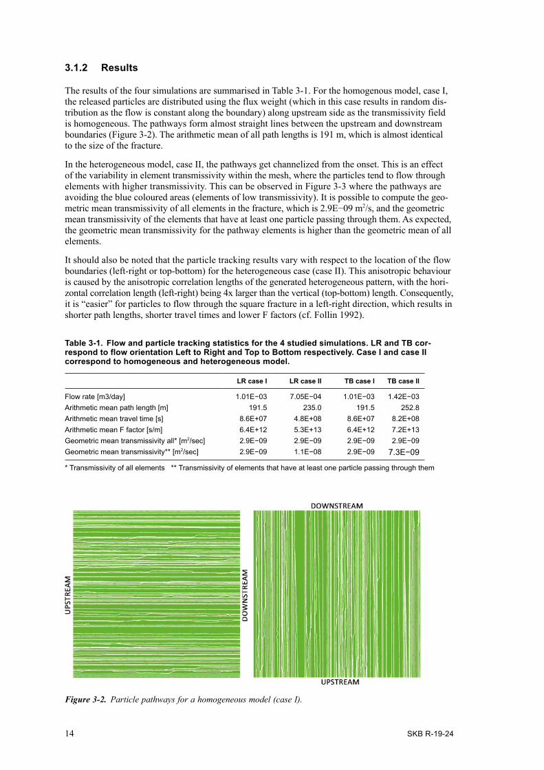
The results of the four simulations are summarised in Table 3-1. For the homogenous model, case I, the released particles are distributed using the flux weight (which in this case results in random dis-tribution as the flow is constant along the boundary) along upstream side as the transmissivity field is homogeneous. The pathways form almost straight lines between the upstream and downstream boundaries (Figure 3-2). The arithmetic mean of all path lengths is 191 m, which is almost identical to the size of the fracture.

In the heterogeneous model, case II, the pathways get channelized from the onset. This is an effect of the variability in element transmissivity within the mesh, where the particles tend to flow through elements with higher transmissivity. This can be observed in Figure 3-3 where the pathways are avoiding the blue coloured areas (elements of low transmissivity). It is possible to compute the geo-metric mean transmissivity of all elements in the fracture, which is 2.9E−09 m2/s, and the geometric mean transmissivity of the elements that have at least one particle passing through them. As expected, the geometric mean transmissivity for the pathway elements is higher than the geometric mean of all elements.

It should also be noted that the particle tracking results vary with respect to the location of the flow boundaries (left-right or top-bottom) for the heterogeneous case (case II). This anisotropic behaviour is caused by the anisotropic correlation lengths of the generated heterogeneous pattern, with the hori-zontal correlation length (left-right) being 4x larger than the vertical (top-bottom) length. Conse quently, it is “easier” for particles to flow through the square fracture in a left-right direction, which results in shorter path lengths, shorter travel times and lower F factors (cf. Follin 1992).

Table 3-1. Flow and particle tracking statistics for the 4 studied simulations. LR and TB cor-respond to flow orientation Left to Right and Top to Bottom respectively. Case I and case II correspond to homogeneous and heterogeneous model.

LR case I LR case II TB case I TB case II

Flow rate [m3/day] 1.01E−03 7.05E−04 1.01E−03 1.42E−03Arithmetic mean path length [m] 191.5 235.0 191.5 252.8Arithmetic mean travel time [s] 8.6E+07 4.8E+08 8.6E+07 8.2E+08Arithmetic mean F factor [s/m] 6.4E+12 5.3E+13 6.4E+12 7.2E+13Geometric mean transmissivity all* [m2/sec] 2.9E−09 2.9E−09 2.9E−09 2.9E−09Geometric mean transmissivity** [m2/sec] 2.9E−09 1.1E−08 2.9E−09 7.3E−09

* Transmissivity of all elements ** Transmissivity of elements that have at least one particle passing through them

Figure 3‑2. Particle pathways for a homogeneous model (case I).

SKB R-19-24 15

For the Left-Right heterogeneous case we compared transmissivity of all elements and elements that have at least one or more particles passing through them. From total of 100 000 elements about 23 000 have at least one particle passing through them. Geometric mean transmissivity of elements with at least one particle is about 5x larger than the average transmissivity of all elements. The results presented in table in Figure 3-4 indicate that the average transmissivity is proportional to the number of particles per element, i.e. elements with more particles tend to have higher transmissivity.

Figure 3‑3. Particle pathways for a heterogeneous model (case II).

Part Element countall

T mean_geo105 048

Number of elements with particle14 000

12 000

10 000

18 000

16 000

14 000

12 000

00 5 10 15 20

Number of particles

Num

ber o

f ele

men

ts

>=1

2,9E-09

23 040

=1 12 612

1,1E-08

=2

6,8E-09

4 982

=3

1,1E-08

2 495

=4

1,9E-08

1 472

=5 801

3,3E-08

>5 678

6,8E-08

1,0E-07

Figure 3‑4. Histogram showing number of elements with corresponding number of passing particles for simulation case “Left-Right_heterogeneous”. In the table on the left the average transmissivity for all elements with corresponding number of particles that pass through them is shown.

16 SKB R-19-24

3.2 Mesh size effect and calibration study

In the first part of this test, a hypothetical DFN model was created and meshed with three different element sizes, while all other properties remained unchanged. This allowed us to study the effect of mesh resolution (element size) on the flow and particle simulation results. In the second part, we calibrated the hydraulic parameters of the coarse mesh model to match results from the fine mesh model using PEST. The results from two realisations (R1a and R1b) are presented in this section.

3.2.1 Model Setup

The model domain was represented by a parallelepiped of a size of 400 x 400 x 800 m3. In the centre of the model domain, a 600 m long vertical borehole is “drilled”. A further five deposition holes were inserted at 400 m depth (Figure 3-5).

Three fracture sets were generated within the model domain, two steeply dipping sets and one gently dipping set based on the data from SDM-Site Forsmark (SKB 2008b, Fox et al. 2007). Geometric fracture set properties are summarised in Table 3-2. Each fracture set is divided into three subsets for fracture sizes from 3-20 m, 20-50 m and 50-200 m.

Model domain

Deposition holes

Borehole

� H = 8 m (-4, +4)

� R = 0.85 m

� c/c = 6 m

� Lx = 400 m (-200, +200)

� Ly = 400 m (-200, +200)

� Lz = 800 m (-200, +200)

� L = 600 m (-300, +300)

800

1 2 3 4 5

Figure 3‑5. Model domain with a vertical borehole and five deposition holes.

SKB R-19-24 17

Table 3-2. Geometrical properties of the three fracture sets.

Set Trend/ Plunge

Fisher k Power law kr rmin rmax P32,o

NNE_EB_3-20 309/2 15 2.6 3 20 0.024066NNE_EB_20-50 309/2 15 2.6 20 50 0.004798NNE_EB_50-200 309/2 15 2.6 50 200 0.003697SH_EB_3-20 5/86 15 2.4 3 20 0.029275SH_EB_20-50 5/86 15 2.4 20 50 0.007909SH_EB_50-200 5/86 15 2.4 50 200 0.007604WNW_EB_3-20 37/4 13 3.1 3 20 0.001534WNW_EB_20-50 37/4 13 3.1 20 50 0.000138WNW_EB_50-200 37/4 13 3.1 50 200 6.2e−005

The hydraulic properties are shown in Table 3-3. Transmissivity is assumed to be directly correlated to the fracture equivalent radius (EqRadius is equal to √(A/π) where A is fracture area) and the fracture aperture is back calculated from the fracture transmissivity. Fracture storativity is calculated only for the sake of completeness (it doesn’t affect the results as all simulations were run at steady state).

Table 3-3. Hydraulic properties of the three fracture sets.

Property Equation Reference

Transmissivity [m2/sec] 1,6E−9 * (EqRadius ^ 0.8) SDM-Site (SKB 2008a)Aperture [m] 0,5 * (Transmissivity ^ 0.5 ) SR-Site (SKB 2011)Storativity [-] 7E−4 * (Transmissivity ^ 0.35) Modified after Rhén et al. (2006)

The generated DFN model needs to fulfil the following two geometrical requirements. Firstly, at least one flow path way from the bottom to the top of a domain must intersect at least one deposition hole. This requirement permits to use the model for particle tracking analysis, where particles are released from a deposition hole. Secondly, the vertical borehole must be intersected by at least 10 fractures which are connected to model outside boundaries. This allows to run PFL simulations and use results for PEST model calibration. If a realisation does not fulfil both requirements it is discarded and not used for further analysis.

For computational efficiency, a “Dead-end” algorithm was applied to the generated stochastic frac-tures. The algorithm removes single dead-end fractures as well as dead-end fracture clusters from all possible pathways between two specified groups of boundaries. In our study for Dead-end algorithm settings, the model domain region was assigned to one boundary group and vertical borehole and deposition holes to another group. For details about the “Dead-end” algorithm refer to FracMan manual (FracMan 2017). The algorithm reduces the number of fractures from about 85 000 fractures to about 9 000, representing roughly 10-20% of the original fractures.

18 SKB R-19-24

3.2.2 Mesh Generation

The connected stochastic fractures were meshed using the MeshMaster® code. Three meshes with different element sizes were created – a coarse mesh with a maximum element size of 10 m, a medium mesh with a maximum element size of 5 m, and a fine mesh with a maximum element size of 2 m (Figure 3-6). Mesh properties including the number of nodes and elements are summarised for two realisations, R1a and R1b, in Table 3-4.

Figure 3‑6. Visualisation of connected fractures for R1a with three different mesh resolutions - a) Coarse b) Medium and c) Fine.

SKB R-19-24 19

Table 3-4. Mesh statistics for two realisations (R1a / R1b).

Mesh # of nodes # of elements Average element area [m2]

Coarse 177 644 / 163 603 307 451 / 281 076 13.2Medium 322 409 / 384 117 589 926 / 711 399 5.2Fine 1 734 978 / 1 619 173 3 346 525 / 3 123 720 1.18

3.2.3 Simulation of a Posiva Flow Log test

The aim of this analysis is to reproduce a steady state Posiva Flow Log (PFL) test. A PFL test is usually conducted from bottom of a hole in specified increments (usually 0.1 – 0.5 m). Results from a PFL test provide information about the cumulative inflow along the tested borehole which can then be converted to inflow at each specific increment.

The simulation was run with constant head boundary conditions. Constant head of +100 m is assigned to all six sides of the model region box and a constant head of +0 m is used in the vertical borehole. As the numerical solution provides flow and pressure head values at any location in a model, it is therefore not necessary to run multiple simulations representing each PFL test increment. Instead one single simulation is sufficient to calculate inflow at each inflow location along the vertical borehole. If the distance between two inflow locations is less than the assumed PFL increment length (0.5 m in our case), the inflow values are added together as they would be measured in a real in-situ PFL test.

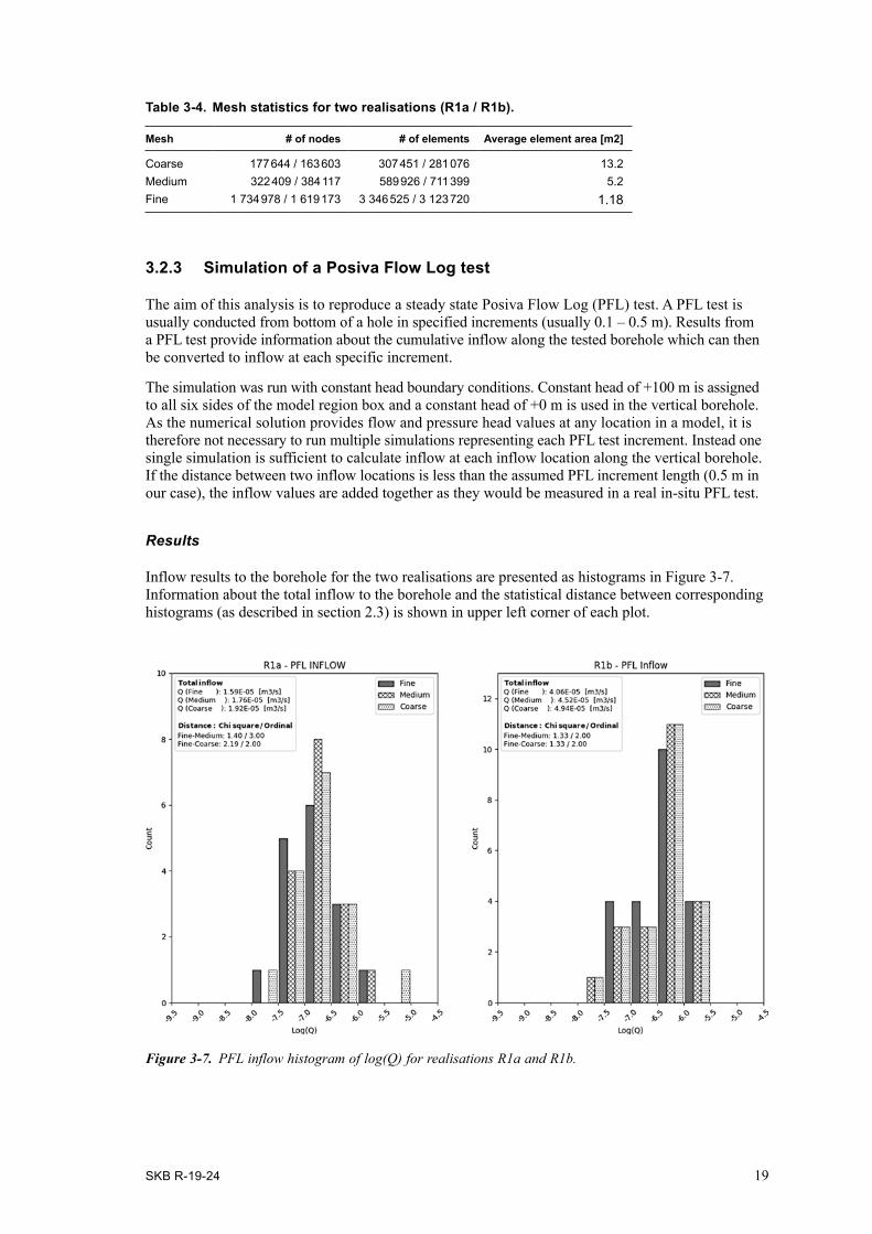
Results

Inflow results to the borehole for the two realisations are presented as histograms in Figure 3-7. Information about the total inflow to the borehole and the statistical distance between corresponding histograms (as described in section 2.3) is shown in upper left corner of each plot.

Figure 3‑7. PFL inflow histogram of log(Q) for realisations R1a and R1b.

20 SKB R-19-24

3.2.4 Particle Tracking

Particle tracking was used to analyse advective transport from the deposition holes to the top surface. As explained above, constant head boundary conditions were assigned to the top and bottom of the parallelepiped, which created a vertical constant head gradient of 5‰ (4 m head difference over 800 m length). Once a steady state solution was reached, 100 particles were released from one of the deposition holes intersected by a connected fracture (if more holes are connected the particles were still released from only single deposition hole) and particle tracking was performed. Results from the particle tracking analyses for both realisations are shown in Figure 3-8. Both realisations yielded similar, but not completely identical, results for all three models. Statistics for all simulations are summarised in Table 3-5.

Table 3-5. Particle tracking statistics for realisations R1a / R1b.

Model Average Time [year] Average Distance [m] Average F Factor [year/m]

Coarse 1.10E−05 / 3.61E−06 949.5 / 742.8 2.64E−01 / 7.64E−02Medium 1.70E−05 / 4.00E−06 1034.7 / 754.9 3.77E−01 / 7.67E−02Fine 1.10E−05 / 3.42E−06 963.9 / 739.0 2.36E−01 / 6.50E−02

Figure 3‑8. Results from the particle tracking analyses showing particle path lengths, travel time and F factor as cumulative distribution functions (CDF).

SKB R-19-24 21

3.2.5 Model calibration using PEST

The capability of the PEST method to calibrate the hydraulic properties of a DFN realisation was studied. The procedure was designed to use PEST to calibrate the transmissivity field of the “Coarse” and “Medium” models to match PFL results of the “Fine” model. In concrete terms, PEST was programmed to estimate fracture transmissivity, correlated to fracture size by parameters b and c in (Equation 5), using two target metrics derived from PFL simulation. The first target used was total inflow to tested borehole and the second target ordinal statistical distance (as described in section 2.3) between inflow histograms. Each PEST calibration iteration consisted of generating a DFN model with transmissivity based on estimated b and c parameters, performing a PFL simulation and compar-ing results to the calibration target.

Equation 3-1

PEST calibrated parameters b and c for “coarse” and “medium” models are summarised in Table 3-6 and visualised in plot in Figure 3-9.

Table 3-6. PEST calibrated parameters for both realisations R1a / R1b.

Model b c

Coarse 1.73 E−09 / 3.29 E−09 0.76 / 0.59Medium 1.52 E−09 / 1.27 E−09 0.80 / 0.84Fine (calibration target) 1.6 E−09 / 1.6 E−09 0.80 / 0.80

Histograms of PFL simulation results are shown in Figure 3-10. In both realisations, a good match between target and calibrated histograms and total inflows was achieved.

3.2.6 Particle tracking using calibrated models

Particle tracking was performed for the PEST calibrated “Coarse” and “Medium” models and the results were compared against the results from particle tracking using the “fine” model (target). The results are shown on Figure 3-11. In both realisations the calibrated models yielded similar results compared to the target model.

1,00E-09

1,00E-08

1,00E-07

1 100

Tran

smis

sivi

ty

10

Equivalent Radius [m]

Transmissivity [m2/s]

Fine Medium R1a Medium R1b Coarse R1a Coarse R1b

Figure 3‑9. Results of transmissivity-size relationship parameters from PEST calibration (cf. Table 7).

22 SKB R-19-24

Figure 3‑10. PFL inflow histogram of log(Q) for realisations R1a and R1b of “Coarse” and “Medium” PEST calibrated models.

Figure 3‑11. Results from particle tracking using PEST calibrated models showing particle path lengths, travel times and F factors as cumulative distribution functions (CDF).

SKB R-19-24 23

3.2.7 Conclusions

Before conducting the main part of the study, the outlined modelling approach described in Chapter 2 was tested. The results from two demonstration (pre-test) studies are presented above. In the first test, we tested if the generated transmissivity patterns give rise to flow channelling. In the second test, we focus on mesh-size effects and PEST calibration performance. The results demonstrated that the out-lined modelling approach worked as intended and yielded reasonable results. Based on the results the following conclusions are drawn:

• We demonstrated that the PEST method can successfully be used as a tool for flow calibration of DFN models.

• We demonstrated that even models with different mesh sizes can be successfully calibrated and give very similar results in terms of flow and particle tracking analyses.

SKB R-19-24 25

4 Comparison of heterogeneous and homogeneous model realisations

4.1 Overview

In this chapter we compare particle tracking results from homogeneous DFN realisations with results from heterogeneous DFN realisations. By a homogeneous DFN realisation we imply that all elements of a fracture have the same transmissivity value and the transmissivity varies only between fractures. In contrast, by a heterogeneous DFN realisation we imply that transmissivity varies at element level so each fracture contains elements with varying properties. In other words, a homogeneous fracture realisation has inter-fracture heterogeneity, whereas a heterogeneous fracture realisation has both inter-fracture and intra-fracture heterogeneity. The ten homogeneous fracture realisations are calibrated on the ten heterogeneous fracture realisations such that the flow to a pumping well in the ith homogeneous realisation is the same as the flow to a pumping well in the ith heterogeneous realisation.

4.2 Workflow

The following list presents the workflow undertaken in our study and the corresponding software used in each step.

1. Ten (10) DFN realisations that fulfil the connectivity requirements were generated. [Fracman]

2. Each DFN realisation was discretised with a fine mesh (small elements). [Fracman + MeshMaster]

3. The fine-mesh realisations were assigned a heterogeneous transmissivity pattern. (Below, realisation with assigned pattern is called “synthetic reality”). [Python]

4. A PFL test was simulated in each of the ten synthetic reality realisations. [Mafic]

5. Particle tracking was simulated in each of the ten synthetic reality realisations. [Mafic]

6. Each of the ten DFN realisations generated in the first step was re-discretised with a coarser mesh (larger elements). This was done to simplify the calibration. [Python].

7. PEST® was used to calibrate the fracture transmissivities in each coarse-mesh DFN realisation. By calibration, we mean that the fracture transmissivities of the coarse-mesh realisation were altered using PEST until a PFL test simulation in the coarse-mesh realisation produced the same flow rate as the PFL test in the fine-mesh (heterogeneous) realisation. [PEST + Python].

8. Particle tracking was simulated in each of the ten calibrated DFN realisations and the results were compared with the particle tracking results (cf. the fifth step above) . [Mafic]

9. Steps 3-8 listed above were repeated four times to study the importance of the chosen hetero geneous transmissivity patterns (synthetic realities). [All]

10. The results were analysed. [Python]

4.3 Model setup

The dimensions of the model domain were 400 m x 400 m x 800 m. In the middle of the domain, a vertical borehole was placed which was used for simulating a PFL test in each realisation. Five cylindrical objects representing deposition holes were placed in the centre of the model. The particle tracking started at the deposition holes. Three fracture sets were generated within the model domain, see Table 4-1.

26 SKB R-19-24

Table 4-1. Geometrical properties of the three fracture sets.

SetTrend/

Plunge Fisher kPower law

kr rmin rmax P32,o

NNE_EB_3-20 309/2 15 2.6 3 20 0.024066NNE_EB_20-50 309/2 15 2.6 20 50 0.004798NNE_EB_50-200 309/2 15 2.6 50 200 0.003697SH_EB_3-20 5/86 15 2.4 3 20 0.029275SH_EB_20-50 5/86 15 2.4 20 50 0.007909SH_EB_50-200 5/86 15 2.4 50 200 0.007604WNW_EB_3-20 37/4 13 3.1 3 20 0.001534WNW_EB_20-50 37/4 13 3.1 20 50 0.000138WNW_EB_50-200 37/4 13 3.1 50 200 6.2e−005

The DFN recipe in Table 4-1 produces a sparse network of approximately 85 000 fractures. The number of fractures used for the flow and transport simulations reported, was optimised by discarding all the dead-end fractures. The algorithm used for the optimisation identifies all possible pathways between specified source and sink boundaries and removes all dead-end fractures and clusters. The optimisation improved the computational efficiency and decreased the number of particles stuck within the particle tracking. The number of active fractures in a model after running the optimisation algorithm decreased to approximately 10-20% of the original number of fractures.

Each of the ten realisations fulfilled the following requirements: a) the vertical borehole had at least 10 inflow locations; b) the top and bottom boundaries of the model domain were interconnected by the fracture network and c) the fracture network connected to at least one of the five deposition holes. Out of a total of 30 generated realisations, ten realisations met the requirements for further

Figure 4‑1. Model domain with a vertical borehole and five deposition holes.

Model domain

Deposition holes

� L x = 400 m (-200, +200)

� L y = 400 m (-200, +200)

� L z = 800 m (-200, +200)

Borehole � L = 600 m (-300, +300)

� H = 8 m (-4, +4)

� R = 0.85 m

� c/c = 6 m

800

1 2 3 4 5

SKB R-19-24 27

analysis. The ten realisations were tessellated with two different resolutions – one “fine” and one “coarse”. A fine mesh realisation had an element size of 2 m and consisted of approximately 3.5 million elements, whereas a coarse mesh realisation had an element size of 5 m and consist of approximately 0.7 million elements.

4.4 Heterogeneity pattern

The Pattern2D algorithm described in section 2.1 was used for generating two heterogeneity patterns. These are referred to below as Pattern A and Pattern B. Each pattern had a size of 200 m x 200 m and a spatial resolution of 1m. Both patterns were generated with an anisotropic covariance function (Equation 6).

, , Equation 4-1

The values of Pattern A were scaled to fall between −2 to 2 and had an arithmetic mean 0.

For Pattern B, a similar technique proposed by Zinn and Harvey (2003) was applied. Starting with pattern A, the 10% of highest and lowest values were truncated. Thereafter the absolute value of the field was calculated which resulted in the extreme values becoming new highs and mean values becoming new lows. The pattern was then scaled to fall between −2 to 2 with an arithmetic mean of −1.1. This pattern is representative of a region with isolated areas of high transmissivity and connected areas of low transmissivity. The patterns are shown in Figure 4-2 and the corresponding histograms of scaled values are shown in Figure 4-3.

Pattern B tends to generate more localized flow channels in comparison to Pattern A. Pattern A has locations with low transmissivity but since they are more isolated, they have lower effect on the channelling. In contrast Pattern B has large connected areas of low transmissivity so the flow is more strongly influenced by the few locations with high transmissivity. Discussion of which pattern better represents the real in-situ fractures is out of the scope of this study.

Figure 4‑2. Visualisation of Pattern A (left) and Pattern B (right).

28 SKB R-19-24

4.5 Hydraulic Model

Pattern A and Pattern B were used to study the effect of heterogeneous hydraulic properties on channelling. Four different synthetic realities (two size-correlated and two uncorrelated) were studied for each of the ten realisations, see Table 4-2. All together 40 synthetic reality realisations were simulated.

Table 4-2: Simulation scenarios

Scenario Transmissivity

Pattern_B+size . .

Pattern_B

Pattern_A+size . .

Pattern_A

Once the transmissivity field was assigned to all elements using the technique described in 2.1, aperture and storativity fields were computed using the equations specified in Table 4-3.

Table 4-3: Fracture sets properties

Property Equation

Transmissivity From scenario case, see Table 4-2Aperture 0.5 * (Transmissivity ^ 0.5)Storativity 7e−4 * (Transmissivity ^ 0.35)

An example of fine-mesh with heterogeneous transmissivity data can be seen in Figure 4-4.

Figure 4‑3. Value histogram of Pattern A (left) and Pattern B (right). Pattern A varies between −2 to 2 and with a mean value of 0. Pattern B varies between −2 to 2 with mean value of −1.1.

SKB R-19-24 29

4.6 Posiva Flow Log Simulation

A Posiva flow log (PFL) simulation was run on each reality realisation. Sequential inflows to the borehole were recorded in a similar manner as in reality, i.e. constant head boundary conditions were used with a head of +100 m on the outside and a head of +0 m in the borehole, see Table 4-4.

Table 4-4: Boundary conditions for simulation of PFL measurements

Geometric object Hydrological boundary

Model region box Constant head +100 mVertical borehole Constant head +0 m

Histograms of the recorded inflows were created for all realisations in each scenario. Figure 4-5 shows an example of such a histogram for realisation R_04. Total inflows to the borehole are shown for the four scenarios in the upper left corner. It should be noted that the total inflow varies between the scenarios, where scenario “Pat_A+size” had the largest inflow and scenario “Pat_B” had the lowest. This relationship was consistent across all reality realisations.

Figure 4‑4. a) DFN model b) Fine mesh with heterogeneous transmissivity data c) Close-up of the mesh.

30 SKB R-19-24

4.7 PEST Calibration

Results from the PFL simulation discussed above were used for the calibration of the homogenous realisations. PEST® in combination with Python scripts was used as a calibration tool. During each PEST® iteration, hydraulic parameters of the coarse mesh were modified and a PFL simulation was performed. The histogram of the PFL test results was compared to the histogram from the reality realisation. After multiple iterations PEST® was able to estimate the best fitted parameters to fulfil the target criteria.

We used two calibration targets in our simulations. Firstly, total inflow to the borehole in a calibrated model should match to inflow from the reality realisation, and secondly, the distance between two histograms of inflow magnitudes should be minimal. At the time of our study we were not sure which method of histogram comparison would work better for the PEST® calibration. For this reason, two different methods were tested; Chi-square distance and ordinal distance as discussed in section 2.3, referred to as PEST-1 and PEST-2 respectively.

It was assumed that the transmissivity field of the calibrated homogeneous model is correlated to fracture size according to (Equation 7. Parameters b and c were calibrated by PEST®.

Equation 4-2

Running an estimation process requires preparation of various setup files for PEST, see Appendix. The files contain information about which estimation method is to be used, estimation parameter ranges, target criteria, etc. In certain cases, PEST is not able to calibrate a model to match target criteria. It is a common practice to modify the setup files and run the estimation process in order to improve the calibration. In our study about one third on the simulations were poorly calibrated.

Figure 4‑5. Results of PFL simulation for all scenarios of reality realisation R_04. Histogram shows number of locations along the tested borehole with corresponding flux.

SKB R-19-24 31

Further optimisation of PEST setup could probably improve the calibration results but this unfortu-nately hasn’t been possible in our study due to the large number of simulations.

4.7.1 PEST® Calibration Results

This chapter summarises the results from the calibration of the homogenous realisations to the heterogeneous reality realisations using the PFL test.

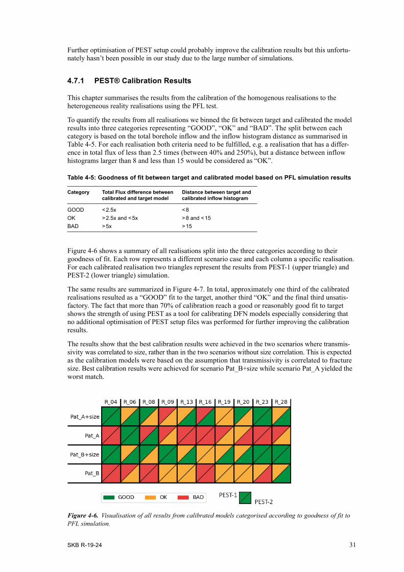
To quantify the results from all realisations we binned the fit between target and calibrated the model results into three categories representing “GOOD”, “OK” and “BAD”. The split between each cate gory is based on the total borehole inflow and the inflow histogram distance as summarised in Table 4-5. For each realisation both criteria need to be fulfilled, e.g. a realisation that has a differ-ence in total flux of less than 2.5 times (between 40% and 250%), but a distance between inflow histograms larger than 8 and less than 15 would be considered as “OK”.

Table 4-5: Goodness of fit between target and calibrated model based on PFL simulation results

Category Total Flux difference between calibrated and target model

Distance between target and calibrated inflow histogram

GOOD < 2.5x < 8OK > 2.5x and < 5x > 8 and < 15BAD > 5x > 15

Figure 4-6 shows a summary of all realisations split into the three categories according to their goodness of fit. Each row represents a different scenario case and each column a specific realisation. For each calibrated realisation two triangles represent the results from PEST-1 (upper triangle) and PEST-2 (lower triangle) simulation.

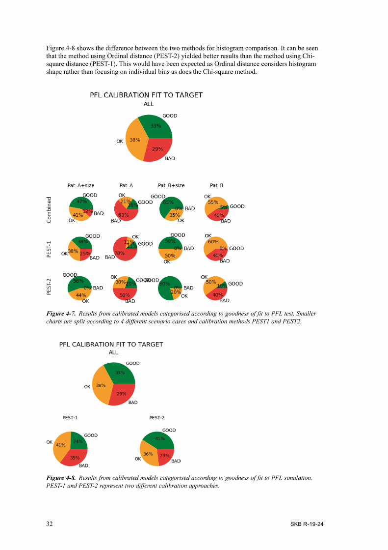
The same results are summarized in Figure 4-7. In total, approximately one third of the calibrated realisations resulted as a “GOOD” fit to the target, another third “OK” and the final third unsatis-factory. The fact that more than 70% of calibration reach a good or reasonably good fit to target shows the strength of using PEST as a tool for calibrating DFN models especially considering that no additional optimisation of PEST setup files was performed for further improving the calibration results.

The results show that the best calibration results were achieved in the two scenarios where transmis-sivity was correlated to size, rather than in the two scenarios without size correlation. This is expected as the calibration models were based on the assumption that transmissivity is correlated to fracture size. Best calibration results were achieved for scenario Pat_B+size while scenario Pat_A yielded the worst match.

Figure 4‑6. Visualisation of all results from calibrated models categorised according to goodness of fit to PFL simulation.

32 SKB R-19-24

Figure 4-8 shows the difference between the two methods for histogram comparison. It can be seen that the method using Ordinal distance (PEST-2) yielded better results than the method using Chi-square distance (PEST-1). This would have been expected as Ordinal distance considers histogram shape rather than focusing on individual bins as does the Chi-square method.

Figure 4‑7. Results from calibrated models categorised according to goodness of fit to PFL test. Smaller charts are split according to 4 different scenario cases and calibration methods PEST1 and PEST2.

Figure 4‑8. Results from calibrated models categorised according to goodness of fit to PFL simulation. PEST-1 and PEST-2 represent two different calibration approaches.

SKB R-19-24 33

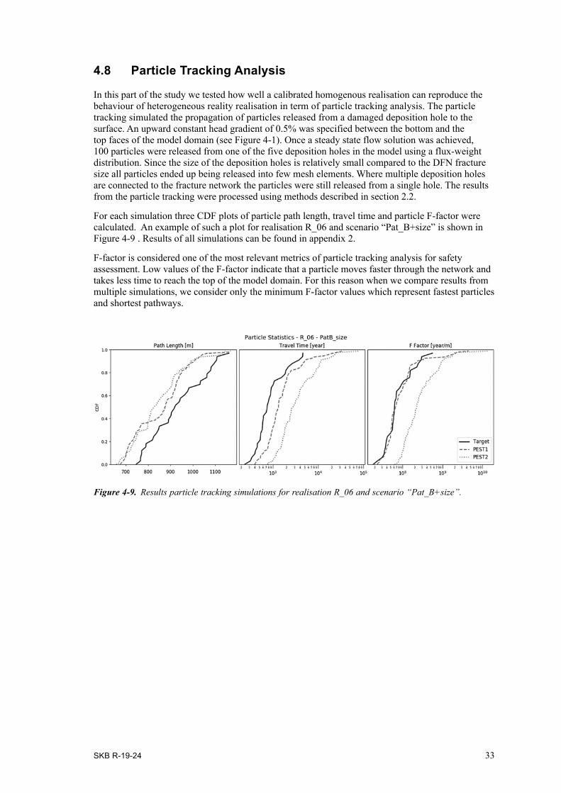
4.8 Particle Tracking Analysis

In this part of the study we tested how well a calibrated homogenous realisation can reproduce the behaviour of heterogeneous reality realisation in term of particle tracking analysis. The particle tracking simulated the propagation of particles released from a damaged deposition hole to the surface. An upward constant head gradient of 0.5% was specified between the bottom and the top faces of the model domain (see Figure 4-1). Once a steady state flow solution was achieved, 100 particles were released from one of the five deposition holes in the model using a flux-weight distribution. Since the size of the deposition holes is relatively small compared to the DFN fracture size all particles ended up being released into few mesh elements. Where multiple deposition holes are connected to the fracture network the particles were still released from a single hole. The results from the particle tracking were processed using methods described in section 2.2.

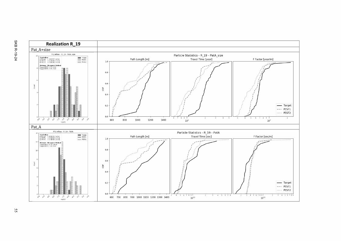
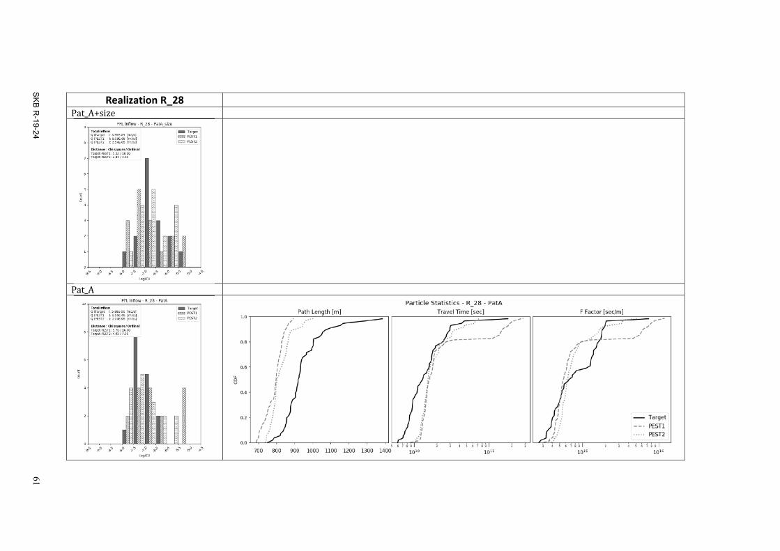
For each simulation three CDF plots of particle path length, travel time and particle F-factor were calculated. An example of such a plot for realisation R_06 and scenario “Pat_B+size” is shown in Figure 4-9 . Results of all simulations can be found in appendix 2.

F-factor is considered one of the most relevant metrics of particle tracking analysis for safety assessment. Low values of the F-factor indicate that a particle moves faster through the network and takes less time to reach the top of the model domain. For this reason when we compare results from multiple simulations, we consider only the minimum F-factor values which represent fastest particles and shortest pathways.

Figure 4‑9. Results particle tracking simulations for realisation R_06 and scenario “Pat_B+size”.

34 SKB R-19-24

Visualisation of all realisations comparing minimum values of F-factor (i.e. the particle with the lowest F-value in the realisation, Fmin) is presented in Figure 4-10. For each calibrated homogeneous realisation the Fmin value is compared against the Fmin value of the heterogeneous reality realisations. If the value of the Fmin of the calibrated homogeneous realisation is more than two times larger than the value of the Fmin of the heterogeneous reality realisation a red triangle pointing upwards is dis played. This indicates a non-conservative prediction of the calibrated homogeneous realisation. If the value of Fmin is two times smaller, a green triangle pointing downwards is shown. This result corresponds to conservative prediction. If Fmin falls between the two previous cases a blue rectangle is displayed. This represents an ideal case, where a calibrated homogeneous realisation yields similar results as the heterogeneous realisation. The background colours for each realisation represent the goodness of fit of the PFL comparisons as described in section 4.7. Since a red background represents simulation where calibration wasn’t successful; comparison of result of particle tracking simulation is meaning-less. In these cases, all symbols are shown in a grey colour. Note that results from four simulations (R_23 and R_28 for Pat_A+size and PatA) are missing due to the numerical error in particle tracking analysis.

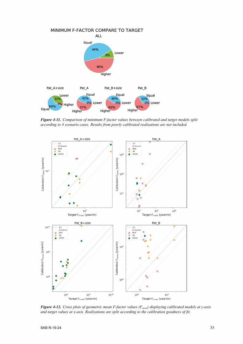
Similar data is plotted in Figure 4-11 where the results are split according to the 4 scenario cases. As already mentioned, results from badly calibrated realisations have no relevance and are therefore excluded from the plots.

Looking at the results, there is a 46% chance that a calibrated homogeneous realisation would yield a non-conservative result (a higher value of the minimum F-factor). About 44% of all calibrated homogeneous realisations yielded virtually identical results and only 9% resulted in conservative results. In scenario case “Pat_A+size” the results from the calibrated models were equal or lower than target and only 7% of realisations yielded non-conservative results. In the other 3 scenarios the possibility that a calibrated model would yield a non-conservative result was about 60 %.

Another way to compare results from particle tracking analysis is to compare the geometric mean of all F-factors (Fmean). Instead of comparing the single fastest particle the average of all tracked particles may be used. It is possible that a calibrated realization could have a higher Fmean and lower Fmin (or opposite) compare the target synthetic reality. Figure 4-12 shows cross-plots where Fmean of reality realisations are plotted on the x-axis and Fmean of calibrated models on the Y-axis. If results from calibrated models correspond, the target data of all points would plot close to a 1:1 line within the 2x bound. If points plot above that line it indicates that a calibrated model has higher value Fmean representing non-conservative results. Results are divided according to classification in section 4.7. With exception of case Pat_A+size, most realisation results plot above the 1:1 line representing a non-conservative model prediction. Results from Pat_A+size also show that a well calibrated realization can yield both conservative and non-conservative Fmean values.

Figure 4‑10. Comparison of minimum F-factor values (Fmin) between calibrated and target models.

SKB R-19-24 35

Figure 4‑11. Comparison of minimum F-factor values between calibrated and target models split according to 4 scenario cases. Results from poorly calibrated realisations are not included.

Figure 4‑12. Cross plots of geometric mean F-factor values (Fmean) displaying calibrated models at y-axis and target values at x-axis. Realizations are split according to the calibration goodness of fit.

SKB R-19-24 37

5 Conclusions

In our study we tried to estimate how well a flow-calibrated homogeneous realisation can reproduce the transport behaviour of heterogeneous realisation. Firstly, we created multiple realisations with heterogeneous fracture properties and performed PFL test simulations. Secondly, we used the results from PFL tests as a calibration target for homogeneous realisations. In the third and last step we ran particle tracking analysis on both realisations and compared the results. Some of the successes of our study are summarised below.

1. We implemented an algorithm, Pattern2D,that can produce channelized flow in a DFN reali-sation. Using pattern2D, we are able to populate any DFN model with data from the generated pattern. This allowed us to further study the effect of channelling by easily modifying patterns which creates intra-fracture heterogeneity in a DFN model.

2. We ran a simulation that mimicked the way a PFL test is performed and were able to use the results for model calibration using PEST®. By introducing a metric called histogram distance we were able to quantify the similarity between two histograms which we applied in our calibra-tion workflow. This technique is not limited to calibration of PFL results and can be used for any calibration to histogram data.

3. We showed that PEST® can be successfully used to calibrate DFN models. Our study shows that using Python scripts it is possible to automate the calibration process based on PEST®, which allows us to calibrate large number of models and reduces man-made induced errors during the process.

4. With a combination of various tools (FracMan, Mafic, ParaView and custom Python classes) we were able to perform transport analyses and quantify and visualise the results.

Examining the results, the general trend was that calibrated homogeneous models tended to produce non-conservative predictions of particle tracking behaviour in comparison to the equivalent hetero-geneous reality realisation. When comparing Fmean it was only the scenario Pat_A+size where the calibrated realizations predicted more conservative results (three conservative against two non-conserv-ative results considering the 2x bound). It is hard to discuss the results for scenarios without size correlations as in general the calibrations were not successful. The difference between Pat_A+size and Pat_B+size could be explained by the fact that Pat_B creates more localized channels (and thus smaller flowing area) compare to Pat_A. For this reason, Pat_A could be better represented by a fracture with homogeneous transmissivity where the particle paths are governed only by fracture boundary conditions (intersection with other fractures).

The difference between the calibrated and target models could be caused by the calibration method. In this study we are calibrating our models to a PFL test in vertical borehole which mostly captures horizontal flow from fracture networks to the tested locations along the borehole. When we are run-ning our particle tracking analyses we assign hydraulic boundaries that create vertical flow through our model, which is mostly dominated by vertical fractures which cannot be tested by a flow test in a vertical borehole.

Another problem arising from testing a fracture with heterogeneous properties is illustrated in Figure 5-1. Two boreholes intersect the fracture at random locations. Since the borehole A intersect the fracture at a location with low transmissivity the inflow to the borehole would be smaller than to Borehole B which detects the fracture at a location with high transmissivity. If we want to model the same fracture using homogeneous properties (as we did in this study) the results would differ depending on which borehole we use as a calibration target.

Statistically if the heterogeneous parameters are normally distributed, a borehole which intersects multiple fractures would sample locations with mostly average values and low and high transmissivity with same probability. This means that a homogeneous model calibrated to the inflows from such a borehole would over predict the transmissivity of some fractures and under predict the transmissivity in others. As we shown in section 3.1 particles tend to travel through pathways with higher transmissivity. Our study showed that it is very difficult (if not impossible) to create a DFN

model with homogeneous properties that would capture the behaviour of high conductive channels and at the same time simulate observed fluxes. As borehole fluxes were used as our calibration target the homogeneous models could miss the behaviour of the high conductive channels. This effect could be tested by applying the same pattern multiple times on the same DFN realization but it was out of the scope of our study.

Transport analyses is a complex task which requires detailed knowledge about local geology and fracture properties. Fracture size parameters are very challenging to derive from the field data but are crucial to the model behaviour. In our study we neglected this large uncertainty by using the same fracture geometry for both the synthetic reality and calibration models and we only focused on fracture hydraulic properties. We showed that even with this geometrical constraint it is challenging to reproduce the effect of channelling observed in in-situ conditions by using simplified homogeneous models. Further research on this probleme is therefore required.

Figure 5‑1. Two vertical boreholes intersecting fracture with heterogeneous hydraulic properties. Borehole A intersects fracture at location with low transmissivity values while borehole B at location with high transmissivity.

SKB R-19-24 39

References

SKB’s (Svensk Kärnbränslehantering AB) publications can be found at www.skb.com/publications.

Andersson J, Hermansson J, Elert M, Gylling B, Moreno L, Selroos J-O, 1998. Derivation and treatment of the flow wetted surface and other geosphere parameters in the transport models FARF31 and COMP23 for use in safety assessment. SKB R-98-60, Svensk Kärnbränslehantering AB.

de Dreuzy J-R, Méheust Y, Pichot V, 2012. Influence of fracture scale heterogeneity on the flow properties of three-dimensional discrete fracture networks (DFN). Journal of Geophysical Research: Solid Earth 117, B11207. doi:10.1029/2012JB009461

Doherty J, 2015. Calibration and uncertainty analysis for complex environmental models. Brisbane: Watermark Numerical Computing.

Follin S, 1992. Numerical calculations on heterogeneity of groundwater flow. SKB TR 92-14, Svensk Kärnbränslehantering AB.

Fox A, La Pointe P, Hermanson J, Öhman J, 2007. Statistical geological discrete fracture network model. Forsmark modelling stage 2.2. SKB R-07-46, Svensk Kärnbränslehantering AB.

FracMan, 2017. User’s manual, Release 7.6. Golder Associates.

Greenwood P E, Nikulin M S, 1996. A guide to chi-squared testing New York: Wiley. (Wiley series in probability and statistics)

Kroese D P, Botev Z I, 2015. Spatial process simulation. In Schmidt V (ed). Stochastic geometry, spatial statistics and random fields: models and algorithms. Cham: Springer. (Lecture notes in mathematics 2120), 369–404.

Makedonska N, Hyman J D, Karra S, Painter S L, Gable C W, Viswanathan H S, 2016. Evaluating the effect of internal aperture variability on transport in kilometer scale discrete fracture networks. Advances in Water Resources 94, 486-497.

Rhén I, Forsmark T, Forssman I, Zetterlund M, 2006. Evaluation of hydrogeological properties for Hydraulic Conductor Domains (HCD) and Hydraulic Rock Domains (HRD). Laxemar subarea – version 1.2. SKB R-06-22, Svensk Kärnbränslehantering AB.

Rubner Y, Tomasi C, Guibas L J, 2000. The Earth Mover’s Distance as a metric for image retrieval, International Journal of Computer Vision 40, 99–121.

SKB, 2008a. Site description of Forsmark at completion of the size investigation phase. SDM-Site Forsmark. SKB TR-08-05, Svensk Kärnbränslehantering AB.

SKB, 2008b. Bedrock hydrogeology Forsmark. Site descriptive modelling, SDM-Site Forsmark. SKB R-08-95, Svensk Kärnbränslehantering AB

SKB, 2011. Long-term safety for the final repository for spent nuclear fuel at Forsmark. Main report of the SR-Site project, volume 1. SKB TR-11-01, Svensk Kärnbränslehantering AB.

Tsang C-F, Neretnieks I, 1998. Flow channeling in heterogeneous fractured rocks. Reviews of Geophysics 36, 275–298.

Tsoflias G, Baker M, Becker M, 2013. Imaging fracture anisotropic flow channeling using GPR signal amplitude and phase. SEG Technical Program Expanded Abstracts 2013, 4428–4433.

Zinn B, Harvey C F, 2003. When good statistical models of aquifer heterogeneity go bad: A comparison of flow, dispersion, and mass transfer in connected and multivariate Gaussian hydraulic conductivity fields. Water Resource Research 39, 1051. doi:10.1029/2001WR001146

Öhberg A, Rouhiainen P, 2000. Posiva groundwater flow measuring techniques. Posiva 2000-12, Posiva Oy, Finland.

SKB R-19-24 41

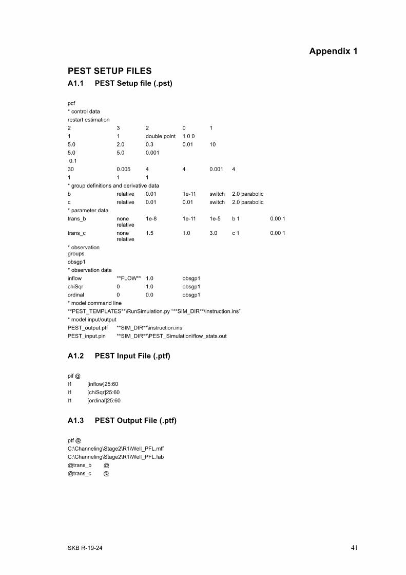
Appendix 1

PEST SETUP FILESA1.1 PEST Setup file (.pst)

pcf* control datarestart estimation2 3 2 0 11 1 double point 1 0 05.0 2.0 0.3 0.01 105.0 5.0 0.001 0.130 0.005 4 4 0.001 41 1 1* group definitions and derivative datab relative 0.01 1e-11 switch 2.0 parabolicc relative 0.01 0.01 switch 2.0 parabolic* parameter datatrans_b none

relative1e-8 1e-11 1e-5 b 1 0.00 1

trans_c none relative

1.5 1.0 3.0 c 1 0.00 1

* observation groupsobsgp1* observation datainflow **FLOW** 1.0 obsgp1 chiSqr 0 1.0 obsgp1ordinal 0 0.0 obsgp1* model command line**PEST_TEMPLATES**\RunSimulation.py “**SIM_DIR**\instruction.ins”* model input/outputPEST_output.ptf **SIM_DIR**\instruction.insPEST_input.pin **SIM_DIR**\PEST_Simulation\flow_stats.out

A1.2 PEST Input File (.ptf)

pif @l1 [inflow]25:60l1 [chiSqr]25:60l1 [ordinal]25:60

A1.3 PEST Output File (.ptf)

ptf @C:\Channeling\Stage2\R1\Well_PFL.mffC:\Channeling\Stage2\R1\Well_PFL.fab@trans_b @ @trans_c @

SKB R-19-24

43

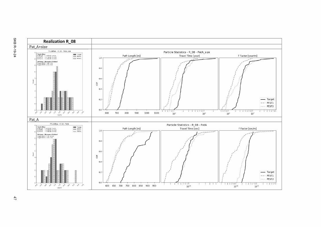
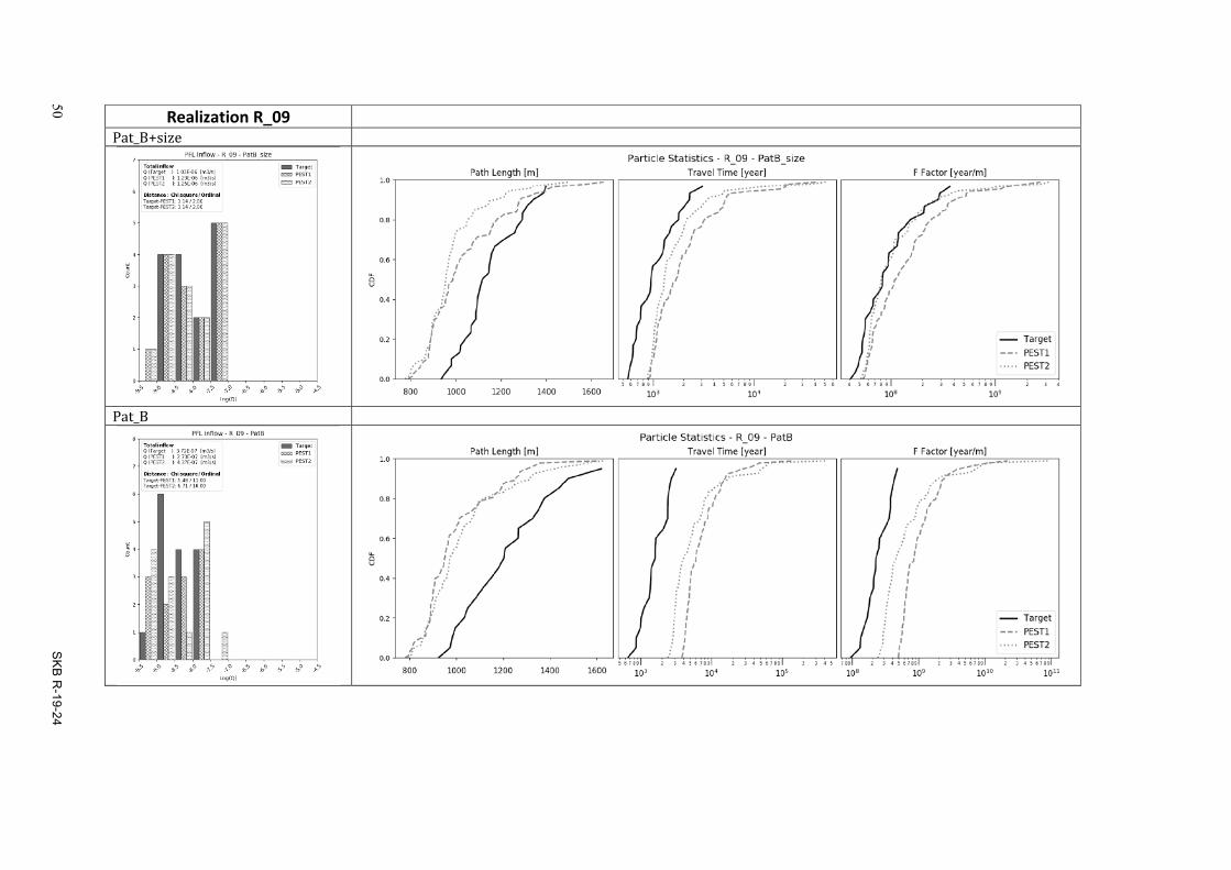
Appendix 2

Simulation results

APPENDIX 2

1

Realization R_04 Pat_A+size

Pat_A

44 SKB R

-19-24

APPENDIX 2

2

Realization R_04 Pat_B+size

Pat_B

SKB R-19-24

45

APPENDIX 2

3


Pat_A

46 SKB R

-19-24

APPENDIX 2

4


Pat_B

SKB R-19-24

47

APPENDIX 2

5


Pat_A

48 SKB R

-19-24

APPENDIX 2

6


Pat_B

SKB R-19-24

49

APPENDIX 2

7


Pat_A

50 SKB R

-19-24

APPENDIX 2

8


Pat_B

SKB R-19-24

51

APPENDIX 2

9


Pat_A

52 SKB R

-19-24

APPENDIX 2

10


Pat_B

SKB R-19-24

53

APPENDIX 2

11


Pat_A

54 SKB R

-19-24

APPENDIX 2

12


Pat_B

SKB R-19-24

55

APPENDIX 2

13


Pat_A

56 SKB R

-19-24

APPENDIX 2

14


Pat_B

SKB R-19-24

57

APPENDIX 2

15


Pat_A

58 SKB R

-19-24

APPENDIX 2

16


Pat_B

SKB R-19-24

59

APPENDIX 2

17


Pat_A

60 SKB R

-19-24

APPENDIX 2

18


Pat_B

SKB R-19-24

61

APPENDIX 2

19


Pat_A

62 SKB R

-19-24

APPENDIX 2

20


Pat_B

Arkite

ktkop

ia AB

, Bro

mm

a, 20

20

SVENSK KÄRNBRÄNSLEHANTERING

SKB is responsible for managing spent nuclear fuel and radioactive

waste produced by the Swedish nuclear power plants such that man

and the environment are protected in the near and distant future.

skb.se

A numerical study of channelling in heterogeneous versus ...

Documents

Transcript of A numerical study of channelling in heterogeneous versus ...