A Numerical Evaluation of Damages Caused by ... - WSEAS · A Numerical Evaluation of Damages Caused...

A Numerical Evaluation of Damages Caused by Asynchronous Motors to the Environment

FRANCESCO MUZI, LUIGI PASSACANTANDO

Department of Electrical Engineering and Computer Science University of L’Aquila

Monteluco di Roio, L’Aquila 67100 ITALY

[email protected] [email protected] Abstract: - In recent years a slow but progressive increase in the world’s temperatures has been consistently recorded. To oppose this global warming trend, two especially important actions are the monitoring and reduction of greenhouse emissions, in large quantity caused by global electric energy production. To this regard an algorithm is proposed to estimate the particles released into the atmosphere as a consequence of the electric energy produced for the operation of asynchronous motors, which in industrialized countries absorb as much as 60 % of the total electric energy generated. The described procedure can also help to evaluate the possibility to supply motors with electric energy produced from renewable sources instead of from thermal power plants supplying traditional public networks, which would of course reduce the environmental impact of motors to almost zero. Emissions linked to electric energy generation were evaluated on the basis of statistics collected from the main electric utilities. The proposed algorithm was validated by means of laboratory tests performed on a single asynchronous motor working under different operating conditions. Key-words: - Electric motor operation and consumption, Emissions and pollution, Environmental sustainability.

1 Introduction In the specialized literature a number of works have dealt with motor energy consumption and efficiency, addressing the geographical distribution and consumption of different kinds of motors as well [1]. In order to improve motor efficiency, many different solutions were proposed, with the basic aim to reduce electric energy absorption while meeting construction constraints and assuring the required performance threshold [2], [12]. Even more so than in the past, attention was recently addressed to digital control strategies and the use of power electronics devices. In this context, particularly successful procedures were adopted, such as the Vector Control (VC) and Scalar Control (HVAC) [3]. On the other hand, also different algorithms were implemented with an aim to increase motor efficiency, following two main research approaches. The former was directed to improve the motor construction features [4], whereas the latter was based on the implementation of control procedures to improve the motor operating performances [5]. In addition, a number of studies were published addressing the errors made in estimating motor efficiency; in this context, the approaches proposed were mainly the Maximum Estimated Error (MEE), the Worst Case Estimated

Error (WCEE), and the Realistic Estimated Error (REE) [6].

2 The problem formulation The issue here was to estimate the amount of emissions into the environment associated to the electric energy drawn by an asynchronous motor. The first step of the proposed procedure is the estimation of the mP mechanical power on the motor shaft:

]W[CP mmm ω⋅= (1)

where ωm is the rotor speed and Cm the electromagnetic torque. Cm can be determined from the dynamic equilibrium equation:

]mN[dt

dJCCC m

Tarm ⋅=−− ω (2)

]mN[dt

dJCCC m

Tarm ⋅++= ω (3)

The quantities Cr, Ca and JT are the load torque, the friction torque and the moment of inertia, respectively; all of them are known quantities. ωm

is an unknown and can be estimated with the algorithm illustrated in Section 4. From the knowledge of ωm, Eq. (3) allows the evaluation of:

WSEAS TRANSACTIONS on CIRCUITS AND SYSTEMS

Francesco Muzi, Luigi Passacantando

ISSN: 1109-2734239

Issue 4, Volume 7, April 2008

]mN[dt

ˆdJCCC m

Tarm ⋅++= ω (4)

The value of mC introduced in Eq. (1) allows the

computation of mP :

]W[ˆCP mmm ω⋅= (5)

Finally, the electric power drawn by the motor can be estimated from the knowledge of the η motor efficiency:

]W[P

P me η

= (6)

η can be read from the motor label or evaluated with laboratory tests. It can also be estimated for an equivalent asynchronous load [10], [11]. The Ee energy supplied by the electrical system can be computed by the following integral:

]sW[dtPEt

0

ee ⋅= ∫ (7)

If the t time is assumed (as a reference) as 1 h, the value obtained from Eq. (7) can be easily expressed in kWh. On the other hand, electricity companies are obliged to write an annual report of their emissions on the basis of 1 kWh of produced energy. The knowledge of the energy required by a single machine for a given industrial working cycle may help to decide how to supply the motor, that is choosing either the external public network or renewable sources available on the premises. Both solutions are shown in Fig. 1.

Motor1 Motor2

Motor1 Motor2

Internal renewable sourceExternal network

External network

1,eP 2,eP

1,eP 2,eP

Fig.1 Example of different arrangements that can be used to supply motors.

Recently, increasing energy production from renewable sources [8], [9], [18] is coming from photovoltaic plants. These generation systems can be subdivided into two main categories:

1. Systems connected to a distribution network (grid-connected systems);

2. Systems completely isolated from the grid (stand-alone systems).

The former system type is shown in Fig. 2.

Fig.2 Photovoltaic grid-connected system. In this case, the electric energy is first converted to the rated frequency and then used to supply the consumer load and/or directly put onto the grid in accordance to a predefined interchange regime [16], [17]. The latter system type is shown in Fig. 3.

Fig.3 Photovoltaic stand-alone system. In this case, the generated energy supplies directly a load while the surplus energy is generally transferred and stored into appropriate batteries

WSEAS TRANSACTIONS on CIRCUITS AND SYSTEMS Francesco Muzi, Luigi Passacantando

ISSN: 1109-2734240


that in their turn will supply the load in absence of solar radiation. Generally speaking, the main components of a photovoltaic system are: a photovoltaic generator (or photovoltaic field for high-power plants), a power controller and conditioner system and an energy storage system (for stand-alone systems). The conversion efficiency of the system takes into account the efficiencies of each component such as: the single photovoltaic cell (solar mono-crystal silicon cells having high purity level are able to transform over 23% of solar energy), solar module, power control and conversion system, and eventually the storage system in the stand-alone plants. In normal conditions, the energy generated by a photovoltaic generator flows to the load and battery simultaneously. When a battery is in discharged condition and the energy required by the load overcomes the generated energy, the photovoltaic generator is connected to a further complementary source that supplies the energy deficit as shown in Fig. 4.

Fig.4 System with a complementary source. A photovoltaic stand-alone system does not have complementary sources to fill the energy deficit. In this case information is required about the nature and amount of energy needs to be satisfied on a daily basis, in different seasons or in one whole year. In such conditions, the proposed algorithm may be very helpful in identifying the best possible solutions.

3 Emissions compared to electric energy production The emissions reported in the following are those released by a traditional thermal power plant. In this case, the emitted pollution can be primarily classified as solid, liquid and gas. Another frequently used classification subdivides the generated pollution as follows:

- emissions into the atmosphere; - avoided CO2 emissions; - outlet water; - hazardous waste.

Emissions into the atmosphere include pollutant particles and greenhouse gases. The former category comprises:

� Sulphur dioxide (SO2); � Nitrogen oxides (NOx); � Powders.

The latter category comprises:

� Carbon dioxide (CO2); � Sulphur hexafluoride (SF6); � Methane (CH4).

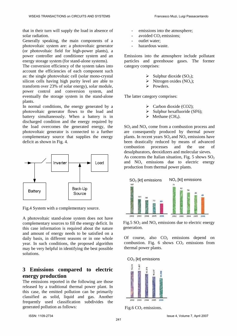
SO2 and NOx come from a combustion process and are consequently produced by thermal power plants. In recent years SO2 and NOx emissions have been drastically reduced by means of advanced combustion processes and the use of desulphurators, deoxidizers and molecular sieves. As concerns the Italian situation, Fig. 5 shows SO2

and NOx emissions due to electric energy production from thermal power plants.

Fig.5 SO2 and NOx emissions due to electric energy generation. Of course, also CO2 emissions depend on combustion. Fig. 6 shows CO2 emissions from thermal power plants.

Fig.6 CO2 emissions.

CO2 [kt] emissions

NOx [kt] emissions SO2 [kt] emissions


ISSN: 1109-2734241


As shown in Fig. 6, in the last few years also CO2

emissions (as SO2 and NOx emissions) have been reduced in Italy. Avoided CO2 emissions can be viewed as a useful indicator in quantifying the penetration level of renewable energy sources. Emissions are often expressed more significantly in [g/kWh] as shown by the diagrams in Figs. 7 and 8.

Fig.7 SO2 and NOx specific emissions.

Fig.8 CO2 specific emissions [g/kWh].

4 The algorithm for motor speed estimation The procedure proposed to estimate the mω motor rotor speed is shown in Fig. 9. The estimate is based on the knowledge of the θ∆ rotor position variation.

( )kϑ∆( )kω

Fig.9 Rotor speed estimator.

The rotor ( )trϑ position, ( )trω speed and ( )tar

acceleration are linked by the following relations:

( ) ( )

( ) ( )

( )

=

=

=

0tadt

d

tatωdt

d

tωtdt

d

r

rr

rrϑ (8)

where ( )tadtd

r

is an additional estimate equation

defining acceleration as a state quantity. In order to implement the model on a DSC (Digital Signal Controller), a discretization of the (8) differential system must be made. Fig. 10 shows a discretization of an ar(t)= a

( constant acceleration

inside the ∆t=t-t0 sampling step.

0t t( )tar

a(

Fig.10 Discretization of a constant rotor acceleration. The result of the discretization procedure is as follows:

( ) ( ) ( )( ) ( )2

112

TaTkkk

rrr

∆+∆−+−= (ωϑϑ (9)

( ) ( ) Takk rr ∆+−= (1ωω (10)

( ) ( ) akaka rr

(=−= 1 (11) where k and k-1 refer to the current and the previous state, respectively. Equations (9), (10) and (11) can be written in a matrix form as:

( )( )( )

( )( )( )

−−−

⋅

∆

∆∆

=

1

1

1

100

102

12

ka

k

k

T

TT

ka

k

k

r

r

r

r

r

r

ωϑ

ωϑ

(12)

Let us define the performed error of the estimate at step k as:

( ) ( ) ( ) ( ) akkaakak rr

(( +=→−= εε (13)

SO2 [g/kWh] NOx [g/kWh]


ISSN: 1109-2734242


Therefore the following relation can be written:

( ) ( ) akkar

(+−=− 11 ε .

Finally, relation (12) can be modified as:

( )( )( )

( )( )( )

+

−−−

⋅

∆

∆∆

=

+

aka

k

k

T

TT

ak

k

k

r

r

r

r

r

((

0

0

1

1

1

100

102

1

0

02

ωϑ

εωϑ (14)

( )( )( )

( )( )( )

aT

T

ka

k

k

T

TT

k

k

k

r

r

r

r

r

(

∆

∆

+

−−−∆

⋅

∆

∆∆

=

∆

0

2

1

1

1

100

102

022

ωϑ

εωϑ (15)

( )( )( )

( )( )( )

aT

T

ka

k

k

T

TT

k

k

k

r

r

r

r

r

(

∆

∆

+

−−−

⋅

∆

∆∆

=

0

2

1

1

1

100

102

122

ωϑ

εωϑ (16)

In order to obtain relations in compact form, the following positions are established:

( )( )( )( )

=k

k

k

kx r

r

εωϑ

;

[ ]

∆

∆∆

=100

102

12

T

TT

A ;

( )( )( )( )

−−−

=−1

1

1

1

ka

k

k

kx

r

r

r

ωϑ

;

∆

∆

=0

2

2

T

T

b ; au(= .

Finally, the model in a compact form can be written as follows:

( ) [ ] ( ) ubkxAkx ⋅+−⋅= 1 State equation (17)

( ) ( )[ ]kky ϑ∆= Output equation (18)

The above model is linear and time-invariant since the matrix coefficients are constant. On the basis of the previous model, an observer based on the Kalman filter can be implemented [13], [17]. Actually, the following non-linear and time-invariant system can be written:

( )( )

+=+= −

kkkk

kkkk

vkuxhy

wkuxfx

,,

,,1 (19)

where:

- kx is the state equation;

- k

y is the output equation;

- f and h are generic equations;

- ku is the input of the system;

- k is the sampling step;

- kw is the noise produced by both disturbances and model accuracies;

- kv is the noise on the output that is linked to the measurement process.

Noises are assumed to be Gaussian with zero mean. The implemented algorithm, which is based on the EKF (Extended Kalman Filter), requires two separate processes:

1. Prediction

kkk abxAx (+= −1ˆ~ (20)

2. Correction

( )kT

kkk xcygxx ~~ˆ −+= (21)

where “g” is the gain vector that is assumed as:

=

3

2

1

g

g

g

g and cT=[1 0 0].

The proposed procedure assumes the

( ) ( ) ( )1−−=∆ kkk ϑϑϑ position change instead of


ISSN: 1109-2734243


the ( )kϑ position as output. In this case, the dynamic equation becomes:

( ) ( ) ( )( ) ( )2

112

TaTkkk rrr

∆+∆−+−= (ωϑϑ (22)

( ) ( ) ( )( ) ( )2

112T

aTkkk rrr

∆+∆−=−− (ωϑϑ (23)

( ) ( ) ( ) ( )( ) ( )2

112T

aTkkkkrrrr

∆+∆−=−−=∆ (ωϑϑϑ (24)

On the other hand, the dynamic equations of speed and acceleration remain unchanged. Consequently the discrete complete model of the position-variation, speed and acceleration can be written as:

( )( )( )

( )( )( )

aT

T

ka

k

k

T

TT

k

k

k

r

r

r

r

r

(

∆

∆

+

−−−∆

⋅

∆

∆∆

=

∆

0

2

1

1

1

100

102

022

ωϑ

εωϑ (25)

Variations will be present only on the state vector of the [A] matrix:

( )( )

( )( )

∆==

k

k

k

kxx r

r

k

εωϑ

[ ]

∆

∆∆

=100

102

02

T

TT

A

Finally, the discrete model becomes:

( ) [ ] ( ) ubkxAkx ⋅+−⋅= 1 (26)

( ) ( )kyky k ϑ∆== (27)

where the output measured quantity corresponds to the position-variation. For the discrete, linear and time-invariant model defined by the (25) matrix equation to be implemented on a DSC, a per unit (p.u.) transformation of the real quantities is required. Therefore equations (20) and (21) can be written in the following form:

( )( )

( )

∆−∆⋅⋅+=

∆−∆⋅⋅+=

∆−∆⋅+∆=∆

pu,kpu,kb

b3pu,kpu,k

pu,kpu,kb

b2pu,kpu,k

pu,kpu,k1pu,kpu,k

~

ag~ˆ

~g~ˆ

~g

~ˆ

ϑϑϑεε

ϑϑωϑωω

ϑϑϑϑ

Fig. 11 shows a flow-chart of the implemented algorithm.

ϑ∆

k1kk abxAx~(+= −

( )kT

kkk x~cygx~x −+=

mω

Fig.11 The implemented algorithm.

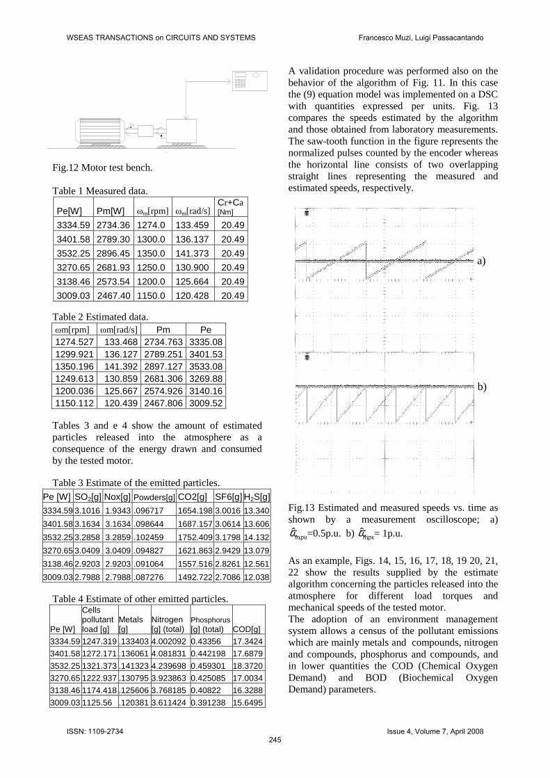
5 Experimental validation of the model Fig. 12 shows the configuration of a laboratory monitoring system that can be adopted to estimate the quantity of emissions released into the environment in consequence of 1kWh energy consumption of one single motor, with data acquisition at the mechanical load side [14]. In laboratory tests the motor speed is measured while in normal cases the speed is estimated using the algorithm of Fig. 11. In order to easily obtain the consumed electric energy in kWh, the operation time of the motor is established as 1h. For certain established mω speeds, Tables 1 and 2 compare data either measured or estimated by a computation based on the implemented speed-estimate algorithm.


ISSN: 1109-2734244


freno a isteresimotore

Fig.12 Motor test bench. Table 1 Measured data.

Pe[W] Pm[W] ωm[rpm] ωm[rad/s] Cr+Ca [Nm]

3334.59 2734.36 1274.0 133.459 20.49

3401.58 2789.30 1300.0 136.137 20.49

3532.25 2896.45 1350.0 141.373 20.49

3270.65 2681.93 1250.0 130.900 20.49

3138.46 2573.54 1200.0 125.664 20.49

3009.03 2467.40 1150.0 120.428 20.49 Table 2 Estimated data. ωm[rpm] ωm[rad/s] Pm Pe 1274.527 133.468 2734.763 3335.08 1299.921 136.127 2789.251 3401.53 1350.196 141.392 2897.127 3533.08 1249.613 130.859 2681.306 3269.88 1200.036 125.667 2574.926 3140.16 1150.112 120.439 2467.806 3009.52

Tables 3 and e 4 show the amount of estimated particles released into the atmosphere as a consequence of the energy drawn and consumed by the tested motor. Table 3 Estimate of the emitted particles.

Pe [W] SO2[g] Nox[g] Powders[g] CO2[g] SF6[g] H2S[g]

3334.59 3.1016 1.9343 .096717 1654.198 3.0016 13.340

3401.58 3.1634 3.1634 .098644 1687.157 3.0614 13.606

3532.25 3.2858 3.2859 .102459 1752.409 3.1798 14.132

3270.65 3.0409 3.0409 .094827 1621.863 2.9429 13.079

3138.46 2.9203 2.9203 .091064 1557.516 2.8261 12.561

3009.03 2.7988 2.7988 .087276 1492.722 2.7086 12.038 Table 4 Estimate of other emitted particles.

Pe [W]

Cells pollutant load [g]

Metals [g]

Nitrogen [g] (total)

Phosphorus [g] (total) COD[g]

3334.59 1247.319 .133403 4.002092 0.43356 17.3424

3401.58 1272.171 .136061 4.081831 0.442198 17.6879

3532.25 1321.373 .141323 4.239698 0.459301 18.3720

3270.65 1222.937 .130795 3.923863 0.425085 17.0034

3138.46 1174.418 .125606 3.768185 0.40822 16.3288

3009.03 1125.56 .120381 3.611424 0.391238 15.6495

A validation procedure was performed also on the behavior of the algorithm of Fig. 11. In this case the (9) equation model was implemented on a DSC with quantities expressed per units. Fig. 13 compares the speeds estimated by the algorithm and those obtained from laboratory measurements. The saw-tooth function in the figure represents the normalized pulses counted by the encoder whereas the horizontal line consists of two overlapping straight lines representing the measured and estimated speeds, respectively.

Fig.13 Estimated and measured speeds vs. time as shown by a measurement oscilloscope; a)

pu,mω =0.5p.u. b) pu,mω = 1p.u.

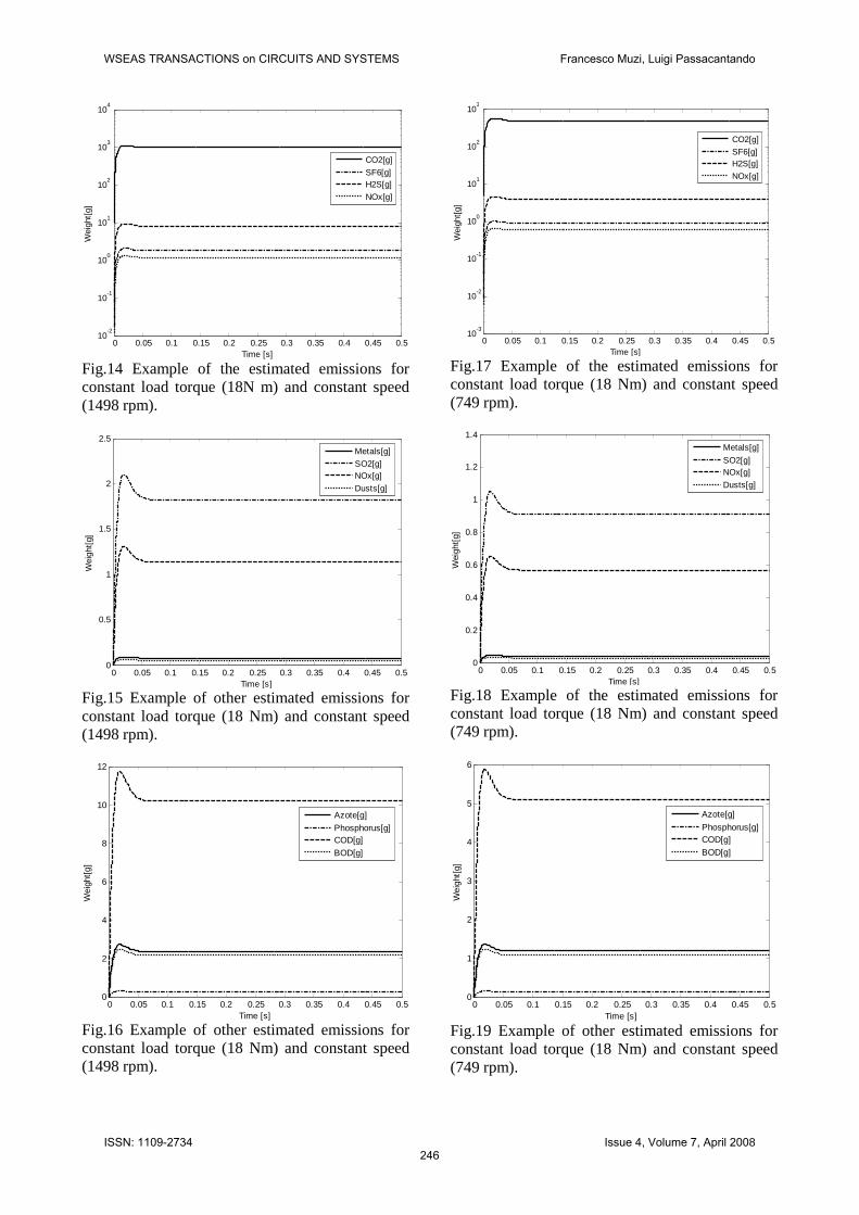
As an example, Figs. 14, 15, 16, 17, 18, 19 20, 21, 22 show the results supplied by the estimate algorithm concerning the particles released into the atmosphere for different load torques and mechanical speeds of the tested motor. The adoption of an environment management system allows a census of the pollutant emissions which are mainly metals and compounds, nitrogen and compounds, phosphorus and compounds, and in lower quantities the COD (Chemical Oxygen Demand) and BOD (Biochemical Oxygen Demand) parameters.

a)

b)


ISSN: 1109-2734245


0 0.05 0.1 0.15 0.2 0.25 0.3 0.35 0.4 0.45 0.510

-2

10-1

100

101

102

103

104

Time [s]

Wei

ght[

g]

CO2[g]

SF6[g]H2S[g]

NOx[g]

Fig.14 Example of the estimated emissions for constant load torque (18N m) and constant speed (1498 rpm).

0 0.05 0.1 0.15 0.2 0.25 0.3 0.35 0.4 0.45 0.50

0.5

1

1.5

2

2.5

Time [s]

Wei

ght[

g]

Metals[g]

SO2[g]NOx[g]

Dusts[g]

Fig.15 Example of other estimated emissions for constant load torque (18 Nm) and constant speed (1498 rpm).

0 0.05 0.1 0.15 0.2 0.25 0.3 0.35 0.4 0.45 0.50

2

4

6

8

10

12

Time [s]

Wei

ght[

g]

Azote[g]

Phosphorus[g]COD[g]

BOD[g]


0 0.05 0.1 0.15 0.2 0.25 0.3 0.35 0.4 0.45 0.510

-3

10-2

10-1

100

101

102

103

Time [s]

Wei

ght[

g]

CO2[g]

SF6[g]H2S[g]

NOx[g]

Fig.17 Example of the estimated emissions for constant load torque (18 Nm) and constant speed (749 rpm).

0 0.05 0.1 0.15 0.2 0.25 0.3 0.35 0.4 0.45 0.50

0.2

0.4

0.6

0.8

1

1.2

1.4

Time [s]

Wei

ght[

g]Metals[g]

SO2[g]NOx[g]

Dusts[g]


0 0.05 0.1 0.15 0.2 0.25 0.3 0.35 0.4 0.45 0.50

1

2

3

4

5

6

Time [s]

Wei

ght[

g]

Azote[g]

Phosphorus[g]COD[g]

BOD[g]



ISSN: 1109-2734246


0 0.05 0.1 0.15 0.2 0.25 0.3 0.35 0.4 0.45 0.510

-3

10-2

10-1

100

101

102

103

Time [s]

Wei

ght[

g]

CO2[g]

SF6[g]H2S[g]

NOx[g]


0 0.05 0.1 0.15 0.2 0.25 0.3 0.35 0.4 0.45 0.50

0.1

0.2

0.3

0.4

0.5

0.6

0.7

Time [s]

Wei

ght[

g]

Metals[g]

SO2[g]NOx[g]

Dusts[g]


0 0.05 0.1 0.15 0.2 0.25 0.3 0.35 0.4 0.45 0.50

0.5

1

1.5

2

2.5

3

3.5

Time [s]

Wei

ght[

g]

Azote[g]

Phosphorus[g]COD[g]

BOD[g]

Fig.22 Example of other estimated emissions for constant load torque (9N m) and constant speed (749 rpm).

6. Conclusions A method was proposed to estimate the amount of polluting emissions due to the production of electric energy required and consumed by asynchronous motors. Since the reduction of atmospheric pollutants is a mandatory issue in national and international directives, a number of measures are constantly being enacted to improve the efficiency of both electric generation and electric end-uses. The method introduced in this paper is based on the Kalman filter estimate and can be used for monitoring purposes as well as to define the best actions targeted at reducing polluting emissions. Moreover, the method allows also to establish when a motor may be supplied by an internal renewable source instead of an external traditional network. The procedure and the suggested algorithm, implemented on a DSC TMS320F2812 from Texas Instrument, were validated by means of laboratory experimental tests. References [1] W. R. Finley, B. Veerkamp., D. Gehring, P.

Hanna, Advantages of Using High Efficiency Motors Such as Nemapremium Around the World, Petroleum and Chemical Industry Technical Conference, 2007, PCIC '07 IEEE, 17-19 Sept. 2007, pp. 1-14.

[2] T. Matsuo, T. A. Lipo, Rotor Design Optimization of Synchronous Reluctance Machine, IEEE Transaction on Energy Conversion, June 1994, Vol.9, pp. 359-365.

[3] F. Abrahamsen, F. Blaabjerg, J. Pedersen, K. Pawel, Z. Grabowski, P. Thøgersen, On the Energy Optimized Control of Standard and High-Efficiency Induction Motors in CT and HVAC Applications, IEEE Transactions on Industry Applications, Jul/Aug 1998, Vol.34, pp. 822-831.

[4] T. Phumiphak, T. Kedsoi and C. Chat-uthai, Energy Management Program for Use of Induction Motors Based on Efficiency Prediction, IEEE Transactions on Industry Applications, Nov/Dec 1997, Vol.33, pp. 1544-1552.

[5] Management Yehia El-Ibiary, An Accurate Low-Cost Method for Determining Electric Motors’ Efficiency for the Purpose of Plant Energy, Petroleum and Chemical Industry Conference 2002, Industry Applications Society 49th, Annual Publication, 2002, pp. 229-235.


ISSN: 1109-2734247


[6] B. Lu, W. Cao, T. G. Habetl, Error Analysis of Motor-Efficiency Estimation and Measurement, Power Electronics Specialists Conference 2007, PESC 2007 IEEE, 17-21 June 2007, pp.612-618.

[7] T. A. Boden, G. Marland, Estimates of Global, Regional, and National Annual CO2

Emissions from Fossil-Fuel Burning, Hydraulic Cement Production, and Gas Flaring: 1950-1992, Environmental Sciences Division Office of Biological and Environmental Research, No.4473, 1995.

[8] S. Kartha, M. Lazarus, M. Bosi, Practical Baseline Recommendations for Greenhouse Gas Mitigation Projects in the Electric Power Sector, OECD and IEA Information Paper, International Energy Agency, May 2002.

[9] Standard CEI EN 60034-2, No.5403, November 1999.

[10] F. Muzi, Numerical Simulation of Induction Motors Dynamic Behaviour - Comparison with Experimental Tests Results, EMTP Newsletter, December 1986.

[11] F. Muzi, A Simplified Model of Induction Motors for Voltage Collapse Studies, Research Report, Department of Electrical Engineering, University of L’Aquila, Italy, No.1-87, January 1987.

[12] C. Bartoletti, G. Fazio, F. Muzi, S. Ricci, G. Sacerdoti, Diagnostics of Electric Power Components: an Improvement on Signal Discrimination, WSEAS Transactions on circuits and systems, Issue 7, Vol.4, July 2005.

[13] F. Muzi, Validation of a Distance Protection Algorithm Based on Kalman Filter, WSEAS Transactions on power systems, Issue 4, Vol.1, April 2006.

[14] F. Muzi, C. Buccione, S. Mautone, A New Architecture for Systems Supplying Essential Loads in the Italian High-Speed Railway (HSR), WSEAS Transactions on Circuits and Systems, Issue 8, Vol.5, August 2006.

[15] F. Muzi, An Alternative FMECA Procedure to Design Distribution System Reliability, WSEAS Transactions on Power Systems, Issue 11, Vol.1, November 2006.

[16] F. Muzi, A Diagnostic Method for Microgrids and Distributed Generation Based on the Parameter State Estimate, International Journal of Circuits, Systems and Signal Processing, ISSN: 1998-0140, Issue 1, Vol.1, 2007.

[17] F. Muzi, A Filtering Procedure Based on Least Squares and Kalman Algorithm for Parameter Estimate in Distance Protection, International Journal of Circuits, Systems and Signal Processing, ISSN: 1998-0140, Issue 1, Vol.1, 2007.

[18] F. Muzi, L. Passacantando, A Real-time Monitoring and Diagnostic Procedure for Electrical Distribution Networks, International Journal of Energy, Issue 2, Vol.1, 2007.


ISSN: 1109-2734248


A Numerical Evaluation of Damages Caused by ... - WSEAS · A Numerical Evaluation of Damages Caused...

Documents

Transcript of A Numerical Evaluation of Damages Caused by ... - WSEAS · A Numerical Evaluation of Damages Caused...