A Novel Approach for Spherical Stereo Vision
237
A Novel Approach for Spherical Stereo Vision of the Faculty of Electrical Engineering and Information Technology at Chemnitz University of Technology approved Dissertation to obtain the academic degree Doktor-Ingenieur Dr.-Ing. submitted by Dipl.-Ing. Michel Findeisen born on 17 November 1979 in Rochlitz filed on 19 February 2015 Assessors: Prof. Dr.-Ing. Gangolf Hirtz Prof. Dr.-Ing. habil. Madhukar Chandra Day of Conferment: 23 April 2015
Transcript of A Novel Approach for Spherical Stereo Vision
A Novel Approach for Spherical Stereo Vision
of the Faculty of Electrical Engineering and Information Technologyat Chemnitz University of Technology
approved
Dissertation
to obtain the academic degree
Doktor-IngenieurDr.-Ing.
submitted
by Dipl.-Ing. Michel Findeisen
born on 17 November 1979 in Rochlitz
filed on 19 February 2015
Assessors: Prof. Dr.-Ing. Gangolf Hirtz
Prof. Dr.-Ing. habil. Madhukar Chandra
Day of Conferment: 23 April 2015


Ein Neuer Ansatz für Sphärisches Stereo Vision
von der Fakutltät für Elektrotechnik und Informationstechnikder Technischen Universität Chemnitz
genehmigte
Dissertation
zur Erlangung des akademischen Grades
Doktor-IngenieurDr.-Ing.
vorgelegt
von Dipl.-Ing. Michel Findeisen
geboren am 17. November 1979 in Rochlitz
eingereicht am 19. Februar 2015
Gutachter: Prof. Dr.-Ing. Gangolf Hirtz
Prof. Dr.-Ing. habil. Madhukar Chandra
Tag der Verleihung: 23. April 2015


Bibliographic Description
Author Michel Findeisen
Title A Novel Approach for Spherical Stereo Vision
OrganizationChemnitz University of Technology, Faculty of Electrical Engineer-ing and Information Technology, Professorship of Digital SignalProcessing and Circuit Technology, PhD Thesis, April 2015
KeywordsStereo Vision; Spherical Stereo Vision; Omnidirectional StereoVision; RGB-D Sensor; Depth Sensing; Trinocular Camera Config-uration; Visual Indoor Surveillance; Fisheye Camera


Abstract
The Professorship of Digital Signal Processing and Circuit Technology of Chemnitz Univer-sity of Technology conducts research in the field of three-dimensional space measurementwith optical sensors. In recent years this field has made major progress.
For example innovative, active techniques such as the “structured light“-principle areable to measure even homogeneous surfaces and have found their way into the consumerelectronic market in terms of Microsofts Kinect® at the present time. Furthermore,high-resolution optical sensors establish powerful, passive stereo vision systems in thefield of indoor surveillance. Thereby they induce new application domains such as securityand assistance systems for domestic environments.
However, the constraint field of view can still be considered as an essential characteristicof all these technologies. For instance, in order to measure a volume in size of a livingspace, two to three deployed 3D sensors have to be applied nowadays. This is due to thefact that the commonly utilized perspective projection principle constrains the visiblearea to a field of view of approximately 120o. On the other hand, novel fish-eye lensesallow the realization of omnidirectional projection models. Therewith, the visible fieldof view can be enlarged up to more than 180o. In combination with a 3D measurementapproach, thus, the number of required sensors for entire room coverage can be reducedconsiderably.
Motivated by the requirements of the field of indoor surveillance, the present workfocuses on the combination of the established stereo vision principle and omnidirectionalprojection methods. The entire 3D measurement of a living space by means of one singlesensor can be considered as major objective.
As a starting point for this thesis, Chapter 1 discusses the underlying requirement,referring to various relevant fields of application. Based on this, the distinct purpose forthe present work is stated.
The necessary mathematical foundations of computer vision are reflected in Chapter2 subsequently. Based on the geometry of the optical imaging process, the projectioncharacteristics of relevant principles are discussed and a generic method for modellingfish-eye cameras is selected.
Chapter 3 deals with the extraction of depth information using classical (perceptivelyimaging) binocular stereo vision configurations. In addition to a complete recap of theprocessing chain, especially occurring measurement uncertainties are investigated.
In the following, Chapter 4 addresses special methods to convert different projectionmodels. The example of mapping an omnidirectional to a perspective projection isemployed in order to develop a method for accelerating this process and, hereby, forreducing the computational load associated therewith. Any errors that occur, as well asthe necessary adjustment of image resolution, are an integral part of the investigation. Asa practical example, an application for person tracking is utilized in order to demonstrateto which extent the usage of “virtual views“ can increase the recognition rate for peopledetectors in the context of omnidirectional monitoring.
Subsequently, an extensive search with respect to omnidirectional imaging stereo visiontechniques is conducted in Chapter 5. It turns out that the complete 3D captureof a room is achievable by the generation of a hemispherical depth map. Therefore,three cameras have to be combined in order to form a trinocular stereo vision system.As a basis for further research, a known trinocular stereo vision method is selected.Furthermore, it is hypothesized that, by applying a modified geometric constellation ofcameras, more precisely in the form of an equilateral triangle, and using an alternativemethod to determine the depth map, the performance can be increased considerably. Anovel method is presented which shall require fewer operations to calculate the distanceinformation and which is to avoid a computational costly step for depth map fusion asnecessary in the comparative method.
In order to evaluate the presented approach as well as the hypotheses, a hemisphericaldepth map is generated in Chapter 6 by means of the new method. Simulation results,based on artificially generated 3D space information and realistic system parameters, arepresented and subjected to a subsequent error estimate.
A demonstrator for generating real measurement information is introduced in Chapter7. In addition, the methods that are applied for calibrating the system intrinsically aswell as extrinsically are explained. It turns out that the calibration procedure utilizedcannot estimate the extrinsic parameters sufficiently. Initial measurements present ahemispherical depth map and thus confirm the operativeness of the concept, but alsoidentify the drawbacks of the calibration used. The current implementation of thealgorithm shows almost real-time behaviour.
Finally, Chapter 8 summarizes the results obtained along the studies and discusses themin the context of comparable binocular and trinocular stereo vision approaches. Forexample the results of the simulations carried out produced a saving of up to 30% in termsof stereo correspondence operations in comparison with a referred trinocular method.Furthermore, the concept introduced allows the avoidance of a weighted averaging step
8

for depth map fusion based on precision values that have to be calculated in a costlymanner. The achievable accuracy is still comparable for both trinocular approaches.
In summary, it can be stated that, in the context of the present thesis, a measurementsystem has been developed which has great potential for future application fields inindustry, security in public spaces as well as home environments.
9


Zusammenfassung
Die Professur Digital- und Schaltungstechnik der Technischen Universität Chemnitzforscht auf dem Gebiet der dreidimensionalen Raumvermessung mittels optischer Sen-sorik. In den letzten Jahren konnte dieses Forschungsgebiet wesentliche Fortschritteverzeichnen.
Beispielsweise erlauben innovative, aktive Verfahren wie das „Structured Light“-Prinzipdie präzise Erfassung auch homogener Oberflächen und halten gegenwärtig in Form derMicrosoft Kinect® Einzug in die Konsumerelektronik. Des Weiteren ermöglichen hochauf-lösende optische Sensoren die Etablierung leistungsfähiger, passiver Stereo-Vision Systemeim Bereich der Raumüberwachung und schaffen damit neuartige Anwendungsfelder wieetwa Sicherheits- und Assistenzsysteme für das häusliche Umfeld.
Eine wesentliche Einschränkung dieser Technologien bildet der nach wie vor stark limi-tierte Sichtbereich der Sensorik. So sind zum Beispiel zur optischen, dreidimensionalenErfassung eines Volumens der Größe eines Wohnraumes aktuell etwa zwei bis drei verteilteSensoren erforderlich. Als Ursache ist hauptsächlich das zugrunde liegende perspektivischeAbbildungsprinzip der 3D-Messverfahren zu nennen, welches den sichtbaren Bereich aufeinen Öffnungswinkel von etwa 120° beschränkt. Neuartige Fischaugenobjektive hinge-gen ermöglichen die Umsetzung omnidirektionaler Projektionsmodelle und damit dieErweiterung des Erfassungsbereichs auf 180° des Sichtfeldes. In Kombination mit einem3D-Messverfahren kann damit die Anzahl der benötigten Sensoren für eine vollständigeRaumvermessung wesentlich reduziert werden.
Motiviert, insbesondere durch die anwendungsbezogenen Anforderungen der Raumüber-wachung, befasst sich die vorliegende Arbeit mit der Kombination des etablierten Stereo-Vision Prinzips mit omnidirektionalen Projektionsverfahren. Das Ziel ist die vollständige,dreidimensionale Erfassung eines Raumes mit nur einem optischen 3D-Sensor.
Als Ausgangspunkt der Arbeit wird in Kapitel 1 die zugrundeliegende Problemstellungin Bezug auf verschiedene, relevante Anwendungsfelder dargelegt. Davon ausgehend wirddas wesentliche Ziel der Untersuchungen formuliert.

Die notwendigen mathematischen Grundlagen des maschinellen Sehens werden anschlie-ßend in Kapitel 2 reflektiert. Ausgehend von der Geometrie des optischen Abbildungs-prozesses werden die Eigenschaften relevanter Projektionsprinzipien erörtert und eingenerisches Verfahren zur Modellierung von Fischaugenkameras ausgewählt.
In Kapitel 3 wird die Gewinnung von Tiefeninformationen unter Verwendung klassischer,perspektivisch abbildender binokularer Stereo-Vision Konfigurationen behandelt. Nebeneiner Aufarbeitung der kompletten Verarbeitungskette werden insbesondere auftretendeMessungenauigkeiten untersucht.
Im Folgenden werden in Kapitel 4 spezielle Verfahren zur Konvertierung verschiedenerProjektionsmodelle diskutiert. Am Beispiel der Transformation einer omnidirektionalenin eine perspektivische Abbildung wird eine Methode entwickelt, welche die damitverbundene Rechenlast reduziert und das Verfahren wesentlich beschleunigt. AuftretendeFehler sowie die notwendige Anpassung der Bildauflösung sind integraler Bestandteil derUntersuchungen. Am Beispiel einer Anwendung zur Personenlokalisierung kann gezeigtwerden, dass sich die Erkennungsrate durch den Einsatz „virtueller Abbildungen“ in deromnidirektionalen Überwachung signifikant steigern lässt.
Aufbauend auf den gelegten Grundlagen wird im sich anschließenden Kapitel 5 eineausführliche Recherche zu omnidirektional abbildenden Stereo-Vision-Verfahren darge-stellt. Es zeigt sich, dass die vollständige 3D-Erfassung eines Raumes mit Hilfe einerhemisphärischen Tiefenkarte möglich ist und dazu prinzipiell drei Kameras zu einemtrinokularen Messsystem kombiniert werden müssen. Als Grundlage für die weiterenUntersuchungen wird ein bekanntes trinokulares Stereo-Vision Verfahren ausgewählt.Davon ausgehend wird die Hypothese aufgestellt, dass bei Änderung der geometrischenKonstellation der Kameras zu einem gleichschenkligen Dreieck sowie Anwendung eineralternativen Methode zur Bestimmung der Tiefenkarte die Performance vergleichsweisesignifikant gesteigert werden kann. Es wird ein neues Verfahren vorgestellt, welchesim Vergleich weniger Operationen zur Berechnung der Entfernungsinformationen benö-tigt und einen rechenaufwändigen Schritt zur Fusionierung von Tiefenkarten, wie imVergleichsverfahren notwendig, unterbinden soll.
Zur Überprüfung des dargelegten Konzeptes und der getroffenen Hypothesen wird inKapitel 6 eine hemisphärische Tiefenkarte auf Grundlage des neuen Verfahrens generiert.Simulationsergebnisse auf Basis künstlich generierter 3D-Rauminformationen und realis-tischer Systemparameter werden präsentiert und einer anschließenden Fehlerabschätzungunterzogen.
Ein Demonstrator zur Erzeugung realer Messinformationen wird in Kapitel 7 vorgestellt.Die verwendeten Methoden zur intrinsischen sowie extrinsischen Kalibrierung des Sys-tems werden dargelegt. Es stellt sich heraus, dass das verwendete Kalibrierverfahren die
12

extrinsischen Parameter nicht genau genug schätzen kann. Erste vorgestellte Messergeb-nisse in Form einer hemisphärischen Tiefenkarte bestätigen die Funktionsfähigkeit desKonzeptes, zeigen aber auch die Nachteile der verwendeten Kalibrierung. Die aktuelleImplementierung des Verfahrens zeigt nahezu Echtzeitverhalten.
Abschließend werden in Kapitel 8 die erreichten Ergebnisse der getätigten Untersuchungenzusammengefasst und im Kontext vergleichbarer binokularer und trinokularer Stereo-Vision Ansätze diskutiert. Beispielsweise zeigen die durchgeführten Simulationen eineEinsparung der Rechenoperationen bei der Bestimmung der Tiefenkarte um bis zu 30%im Vergleich zum Referenzverfahren. Weiterführend kann im vorgestellten Konzept beider Fusionierung von Entfernungsinformationen auf eine gewichtete Mittelwertbildungunter Verwendung aufwendig zu berechnender Genauigkeitswerte verzichtet werden. Dieerreichbare Präzision ist dennoch für beide trinokulare Verfahren vergleichbar.
Zusammenfassend kann gesagt werden, dass im Rahmen der vorliegenden Arbeit einMesssystem entstanden ist, welches großes Potenzial für zukünftige Aufgabenfelder inIndustrie, der Sicherheit im öffentlichen Raum sowie im häuslichen Bereich aufweist.
13


Contents
Abstract 7
Zusammenfassung 11
Acronyms 27
Symbols 29
Acknowledgement 33
1 Introduction 351.1 Visual Surveillance . . . . . . . . . . . . . . . . . . . . . . . . . . . . . . . 351.2 Challenges in Visual Surveillance . . . . . . . . . . . . . . . . . . . . . . . 381.3 Outline of the Thesis . . . . . . . . . . . . . . . . . . . . . . . . . . . . . . 41
2 Fundamentals of Computer Vision Geometry 432.1 Projective Geometry . . . . . . . . . . . . . . . . . . . . . . . . . . . . . . 43
2.1.1 Euclidean Space . . . . . . . . . . . . . . . . . . . . . . . . . . . . 432.1.2 Projective Space . . . . . . . . . . . . . . . . . . . . . . . . . . . . 44
2.2 Camera Geometry . . . . . . . . . . . . . . . . . . . . . . . . . . . . . . . 452.2.1 Geometrical Imaging Process . . . . . . . . . . . . . . . . . . . . . 45
2.2.1.1 Projection Models . . . . . . . . . . . . . . . . . . . . . . 462.2.1.2 Intrinsic Model . . . . . . . . . . . . . . . . . . . . . . . . 472.2.1.3 Extrinsic Model . . . . . . . . . . . . . . . . . . . . . . . 502.2.1.4 Distortion Models . . . . . . . . . . . . . . . . . . . . . . 51
2.2.2 Pinhole Camera Model . . . . . . . . . . . . . . . . . . . . . . . . . 512.2.2.1 Complete Forward Model . . . . . . . . . . . . . . . . . . 522.2.2.2 Back Projection . . . . . . . . . . . . . . . . . . . . . . . 53
2.2.3 Equiangular Camera Model . . . . . . . . . . . . . . . . . . . . . . 542.2.4 Generic Camera Models . . . . . . . . . . . . . . . . . . . . . . . . 55
2.2.4.1 Complete Forward Model . . . . . . . . . . . . . . . . . . 562.2.4.2 Back Projection . . . . . . . . . . . . . . . . . . . . . . . 58
15
Contents
2.3 Camera Calibration Methods . . . . . . . . . . . . . . . . . . . . . . . . . 582.3.1 Perspective Camera Calibration . . . . . . . . . . . . . . . . . . . . 592.3.2 Omnidirectional Camera Calibration . . . . . . . . . . . . . . . . . 59
2.4 Two-View Geometry . . . . . . . . . . . . . . . . . . . . . . . . . . . . . . 602.4.1 Epipolar Geometry . . . . . . . . . . . . . . . . . . . . . . . . . . . 612.4.2 The Fundamental Matrix . . . . . . . . . . . . . . . . . . . . . . . 632.4.3 Epipolar Curves . . . . . . . . . . . . . . . . . . . . . . . . . . . . 64
3 Fundamentals of Stereo Vision 673.1 Introduction . . . . . . . . . . . . . . . . . . . . . . . . . . . . . . . . . . . 67
3.1.1 The Concept Stereo Vision . . . . . . . . . . . . . . . . . . . . . . 673.1.2 Overview of a Stereo Vision Processing Chain . . . . . . . . . . . . 68
3.2 Stereo Calibration . . . . . . . . . . . . . . . . . . . . . . . . . . . . . . . 693.2.1 Extrinsic Stereo Calibration With Respect to the Projective Error 70
3.3 Stereo Rectification . . . . . . . . . . . . . . . . . . . . . . . . . . . . . . . 723.3.1 A Compact Algorithm for Rectification of Stereo Pairs . . . . . . . 73
3.4 Stereo Correspondence . . . . . . . . . . . . . . . . . . . . . . . . . . . . . 763.4.1 Disparity Computation . . . . . . . . . . . . . . . . . . . . . . . . 763.4.2 The Correspondence Problem . . . . . . . . . . . . . . . . . . . . . 77
3.5 Triangulation . . . . . . . . . . . . . . . . . . . . . . . . . . . . . . . . . . 793.5.1 Depth Measurement . . . . . . . . . . . . . . . . . . . . . . . . . . 793.5.2 Range Field of Measurement . . . . . . . . . . . . . . . . . . . . . 803.5.3 Measurement Accuracy . . . . . . . . . . . . . . . . . . . . . . . . 803.5.4 Measurement Errors . . . . . . . . . . . . . . . . . . . . . . . . . . 81
3.5.4.1 Quantization Error . . . . . . . . . . . . . . . . . . . . . 823.5.4.2 Statistical Distribution of Quantization Errors . . . . . . 83
4 Virtual Cameras 874.1 Introduction and Related Works . . . . . . . . . . . . . . . . . . . . . . . 884.2 Omni to Perspective Vision . . . . . . . . . . . . . . . . . . . . . . . . . . 90
4.2.1 Forward Mapping . . . . . . . . . . . . . . . . . . . . . . . . . . . 904.2.2 Backward Mapping . . . . . . . . . . . . . . . . . . . . . . . . . . . 934.2.3 Fast Backward Mapping . . . . . . . . . . . . . . . . . . . . . . . . 96
4.3 Error Analysis . . . . . . . . . . . . . . . . . . . . . . . . . . . . . . . . . 994.4 Accuracy Analysis . . . . . . . . . . . . . . . . . . . . . . . . . . . . . . . 101
4.4.1 Intrinsics of the Source Camera . . . . . . . . . . . . . . . . . . . . 1024.4.2 Intrinsics of the Target Camera . . . . . . . . . . . . . . . . . . . . 1024.4.3 Marginal Virtual Pixel Size . . . . . . . . . . . . . . . . . . . . . . 104
4.5 Performance Measurements . . . . . . . . . . . . . . . . . . . . . . . . . . 1094.6 Virtual Perspective Views for Real-Time People Detection . . . . . . . . . 110
16

Contents
5 Omnidirectional Stereo Vision 1135.1 Introduction and Related Works . . . . . . . . . . . . . . . . . . . . . . . 113
5.1.1 Geometrical Configuration . . . . . . . . . . . . . . . . . . . . . . . 1165.1.1.1 H-Binocular Omni-Stereo with Panoramic Views . . . . . 1175.1.1.2 V-Binocular Omnistereo with Panoramic Views . . . . . 1195.1.1.3 Binocular Omnistereo with Hemispherical Views . . . . . 1205.1.1.4 Trinocular Omnistereo . . . . . . . . . . . . . . . . . . . 1225.1.1.5 Miscellaneous Configurations . . . . . . . . . . . . . . . . 125
5.2 Epipolar Rectification . . . . . . . . . . . . . . . . . . . . . . . . . . . . . 1265.2.1 Cylindrical Rectification . . . . . . . . . . . . . . . . . . . . . . . . 1275.2.2 Epipolar Equi-Distance Rectification . . . . . . . . . . . . . . . . . 1285.2.3 Epipolar Stereographic Rectification . . . . . . . . . . . . . . . . . 1285.2.4 Comparison of Rectification Methods . . . . . . . . . . . . . . . . 129
5.3 A Novel Spherical Stereo Vision Setup . . . . . . . . . . . . . . . . . . . . 1295.3.1 Physical Omnidirectional Camera Configuration . . . . . . . . . . 1315.3.2 Virtual Rectified Cameras . . . . . . . . . . . . . . . . . . . . . . . 131
6 A Novel Spherical Stereo Vision Algorithm 1356.1 Matlab Simulation Environment . . . . . . . . . . . . . . . . . . . . . . . 1356.2 Extrinsic Configuration . . . . . . . . . . . . . . . . . . . . . . . . . . . . 1366.3 Physical Camera Configuration . . . . . . . . . . . . . . . . . . . . . . . . 1376.4 Virtual Camera Configuration . . . . . . . . . . . . . . . . . . . . . . . . . 137
6.4.1 The Focal Length . . . . . . . . . . . . . . . . . . . . . . . . . . . 1386.4.2 Prediscussion of the Field of View . . . . . . . . . . . . . . . . . . 1386.4.3 Marginal Virtual Pixel Sizes . . . . . . . . . . . . . . . . . . . . . . 1396.4.4 Calculation of the Field of View . . . . . . . . . . . . . . . . . . . 1426.4.5 Calculation of the Virtual Pixel Size Ratios . . . . . . . . . . . . . 1436.4.6 Results of the Virtual Camera Parameters . . . . . . . . . . . . . . 144
6.5 Spherical Depth Map Generation . . . . . . . . . . . . . . . . . . . . . . . 1476.5.1 Omnidirectional Imaging Process . . . . . . . . . . . . . . . . . . . 1486.5.2 Rectification Process . . . . . . . . . . . . . . . . . . . . . . . . . . 1486.5.3 Rectified Depth Map Generation . . . . . . . . . . . . . . . . . . . 1506.5.4 Spherical Depth Map Generation . . . . . . . . . . . . . . . . . . . 1516.5.5 3D Reprojection . . . . . . . . . . . . . . . . . . . . . . . . . . . . 153
6.6 Error Analysis . . . . . . . . . . . . . . . . . . . . . . . . . . . . . . . . . 154
7 Stereo Vision Demonstrator 1637.1 Physical System Setup . . . . . . . . . . . . . . . . . . . . . . . . . . . . . 1637.2 System Calibration Strategy . . . . . . . . . . . . . . . . . . . . . . . . . . 165
7.2.1 Intrinsic Calibration of the Physical Cameras . . . . . . . . . . . . 165
17

Contents
7.2.2 Extrinsic Calibration of the Physical and the Virtual Cameras . . 1667.2.2.1 Extrinsic Initialization of the Physical Cameras . . . . . 1677.2.2.2 Extrinsic Initialization of the Virtual Cameras . . . . . . 1677.2.2.3 Two-View Stereo Calibration and Rectification . . . . . . 1677.2.2.4 Three-View Stereo Rectification . . . . . . . . . . . . . . 1687.2.2.5 Extrinsic Calibration Results . . . . . . . . . . . . . . . . 169
7.3 Virtual Camera Setup . . . . . . . . . . . . . . . . . . . . . . . . . . . . . 1717.4 Software Realization . . . . . . . . . . . . . . . . . . . . . . . . . . . . . . 1727.5 Experimental Results . . . . . . . . . . . . . . . . . . . . . . . . . . . . . . 172
7.5.1 Qualitative Assessment . . . . . . . . . . . . . . . . . . . . . . . . 1727.5.2 Performance Measurements . . . . . . . . . . . . . . . . . . . . . . 174
8 Discussion and Outlook 1778.1 Discussion of the Current Results and Further Need for Research . . . . . 177
8.1.1 Assessment of the Geometrical Camera Configuration . . . . . . . 1788.1.2 Assessment of the Depth Map Computation . . . . . . . . . . . . . 1798.1.3 Assessment of the Depth Measurement Error . . . . . . . . . . . . 1828.1.4 Assessment of the Spherical Stereo Vision Demonstrator . . . . . . 183
8.2 Review of the Different Approaches for Hemispherical Depth Map Generation1848.2.1 Comparison of the Equilateral and the Right-Angled Three-View
Approach . . . . . . . . . . . . . . . . . . . . . . . . . . . . . . . . 1848.2.2 Review of the Three-View Approach in Comparison with the Two-
View Method . . . . . . . . . . . . . . . . . . . . . . . . . . . . . . 1858.3 A Sample Algorithm for Human Behaviour Analysis . . . . . . . . . . . . 1878.4 Closing Remarks . . . . . . . . . . . . . . . . . . . . . . . . . . . . . . . . 189
A Relevant Mathematics 191A.1 Cross Product by Skew Symmetric Matrix . . . . . . . . . . . . . . . . . . 191A.2 Derivation of the Quantization Error . . . . . . . . . . . . . . . . . . . . . 191A.3 Derivation of the Statistical Distribution of Quantization Errors . . . . . . 192A.4 Approximation of the Quantization Error for Equiangular Geometry . . . 194
B Further Relevant Publications 197B.1 H-Binocular Omnidirectional Stereo Vision with Panoramic Views . . . . 197B.2 V-Binocular Omnidirectional Stereo Vision with Panoramic Views . . . . 198B.3 Binocular Omnidirectional Stereo Vision with Hemispherical Views . . . . 200B.4 Trinocular Omnidirectional Stereo Vision . . . . . . . . . . . . . . . . . . 201B.5 Miscellaneous Configurations . . . . . . . . . . . . . . . . . . . . . . . . . 202
Bibliography 209
List of Figures 223
18

Contents
List of Tables 229
Affidavit 231
Theses 233
Thesen 235
Curriculum Vitae 237
19


Inhaltsverzeichnis
Zusammenfassung (englisch) 7
Zusammenfassung (deutsch) 11
Abkürzungsverzeichnis 27
Symbolverzeichnis 29
Danksagung 33
1 Einleitung 351.1 Optische Überwachung . . . . . . . . . . . . . . . . . . . . . . . . . . . . . 351.2 Herausforderungen bei der Optischen Überwachung . . . . . . . . . . . . . 381.3 Überblick über die Arbeit . . . . . . . . . . . . . . . . . . . . . . . . . . . 41
2 Geometrische Grundlagen des Maschinellen Sehens 432.1 Projektive Geometrie . . . . . . . . . . . . . . . . . . . . . . . . . . . . . . 43
2.1.1 Euklidischer Raum . . . . . . . . . . . . . . . . . . . . . . . . . . . 432.1.2 Projektiver Raum . . . . . . . . . . . . . . . . . . . . . . . . . . . 44
2.2 Kamera Geometrie . . . . . . . . . . . . . . . . . . . . . . . . . . . . . . . 452.2.1 Geometrischer Abbildungsprozess . . . . . . . . . . . . . . . . . . . 45
2.2.1.1 Projektionsmodelle . . . . . . . . . . . . . . . . . . . . . 462.2.1.2 Intrinsisches Modell . . . . . . . . . . . . . . . . . . . . . 472.2.1.3 Extrinsisches Modell . . . . . . . . . . . . . . . . . . . . . 502.2.1.4 Verzerrungsmodell . . . . . . . . . . . . . . . . . . . . . . 51
2.2.2 Lochkameramodell . . . . . . . . . . . . . . . . . . . . . . . . . . . 512.2.2.1 Vollständiges Vorwärtsmodell . . . . . . . . . . . . . . . . 522.2.2.2 Rückprojektion . . . . . . . . . . . . . . . . . . . . . . . . 53
2.2.3 Equiangulares Kameramodell . . . . . . . . . . . . . . . . . . . . . 542.2.4 Generische Kameramodelle . . . . . . . . . . . . . . . . . . . . . . 55
2.2.4.1 Vollständiges Vorwärtsmodell . . . . . . . . . . . . . . . . 562.2.4.2 Rückprojektion . . . . . . . . . . . . . . . . . . . . . . . . 58
21

Contents
2.3 Kamerakalibrierverfahren . . . . . . . . . . . . . . . . . . . . . . . . . . . 582.3.1 Perspektivische Kamerakalibrierung . . . . . . . . . . . . . . . . . 592.3.2 Omnidirektionale Kamerakalibrierung . . . . . . . . . . . . . . . . 59
2.4 Zwei-Kamera Geometrie . . . . . . . . . . . . . . . . . . . . . . . . . . . . 602.4.1 Epipolargeometrie . . . . . . . . . . . . . . . . . . . . . . . . . . . 612.4.2 Die Fundamentalmatrix . . . . . . . . . . . . . . . . . . . . . . . . 632.4.3 Epipolarkurven . . . . . . . . . . . . . . . . . . . . . . . . . . . . . 64
3 Die Grundlagen des Stereo Vision Verfahrens 673.1 Einleitung . . . . . . . . . . . . . . . . . . . . . . . . . . . . . . . . . . . . 67
3.1.1 Das Konzept Stereo Vision . . . . . . . . . . . . . . . . . . . . . . 673.1.2 Überblick über die Stereo Vision Prozesskette . . . . . . . . . . . . 68
3.2 Stereokalibrierung . . . . . . . . . . . . . . . . . . . . . . . . . . . . . . . 693.2.1 Extrinsiche Stereokalibrierung . . . . . . . . . . . . . . . . . . . . 70
3.3 Stereorektifizierung . . . . . . . . . . . . . . . . . . . . . . . . . . . . . . . 723.3.1 Ein Kompakter Algorithmus für die Rektifizierung von Stereopaaren 73
3.4 Stereokorrespondenz . . . . . . . . . . . . . . . . . . . . . . . . . . . . . . 763.4.1 Disparitätsberechnung . . . . . . . . . . . . . . . . . . . . . . . . . 763.4.2 Das Korrespondenzproblem . . . . . . . . . . . . . . . . . . . . . . 77
3.5 Triangulation . . . . . . . . . . . . . . . . . . . . . . . . . . . . . . . . . . 793.5.1 Entfernungsbestimmung . . . . . . . . . . . . . . . . . . . . . . . . 793.5.2 Grenzen des Messfeldes . . . . . . . . . . . . . . . . . . . . . . . . 803.5.3 Messgenauigkeit . . . . . . . . . . . . . . . . . . . . . . . . . . . . 803.5.4 Messfehler . . . . . . . . . . . . . . . . . . . . . . . . . . . . . . . . 81
3.5.4.1 Quantisierungsfehler . . . . . . . . . . . . . . . . . . . . . 823.5.4.2 Statistische Verteilung des Quantisierungsfehlers . . . . . 83
4 Virtuelle Kameras 874.1 Einleitung und Relevante Veröffentlichungen . . . . . . . . . . . . . . . . . 884.2 Von der Omnidirektionalen zur Perspektivischen Abbildung . . . . . . . . 90
4.2.1 Vorwärtverfahren . . . . . . . . . . . . . . . . . . . . . . . . . . . . 904.2.2 Rückwärtsverfahren . . . . . . . . . . . . . . . . . . . . . . . . . . 934.2.3 Schnelles Rückwärtsverfahren . . . . . . . . . . . . . . . . . . . . . 96
4.3 Fehleranalyse . . . . . . . . . . . . . . . . . . . . . . . . . . . . . . . . . . 994.4 Analyse der Genauigkeit . . . . . . . . . . . . . . . . . . . . . . . . . . . . 101
4.4.1 Die Intrinsischen Parameter der Physikalischen Kamera . . . . . . 1024.4.2 Die Intrinsischen Parameter der Virtuellen Kamera . . . . . . . . . 1024.4.3 Grenzpixelgröße . . . . . . . . . . . . . . . . . . . . . . . . . . . . 104
4.5 Geschwindigkeitsmessungen . . . . . . . . . . . . . . . . . . . . . . . . . . 1094.6 Virtuelle Perspektivische Ansichten für eine Echtzeit-Personenerkennung . 110
22
Contents
5 Omnidirektionales Stereo Vision 1135.1 Einleitung und Relevante Veröffentlichungen . . . . . . . . . . . . . . . . . 113
5.1.1 Geometrische Konfiguration . . . . . . . . . . . . . . . . . . . . . . 1165.1.1.1 H-Binokulares Omnidirektionales Stereo Vision mit Pan-
oramischer Abbildung . . . . . . . . . . . . . . . . . . . . 1175.1.1.2 V-Binokulares Omnidirektionales Stereo Vision mit Pan-
oramischer Abbildung . . . . . . . . . . . . . . . . . . . . 1195.1.1.3 Binokulares Omnidirektionales Stereo Vision mit Hemi-
sphärischer Abbildung . . . . . . . . . . . . . . . . . . . . 1205.1.1.4 Trinokulares Omnidirektionales Stereo Vision . . . . . . . 1225.1.1.5 Sonstige Konfigurationen . . . . . . . . . . . . . . . . . . 125
5.2 Epipolare Rektifizierungsverfahren . . . . . . . . . . . . . . . . . . . . . . 1265.2.1 Zylindrische Rektifizierung . . . . . . . . . . . . . . . . . . . . . . 1275.2.2 Epipolare Equidistante Rektifizierung . . . . . . . . . . . . . . . . 1285.2.3 Epipolare Stereographische Rektifizierung . . . . . . . . . . . . . . 1285.2.4 Vergleich der Rektifizierungsmethoden . . . . . . . . . . . . . . . . 129
5.3 Ein Neuartiges Stereo Vision Setup . . . . . . . . . . . . . . . . . . . . . . 1295.3.1 Physikalische Omnidirektionale Kamerakonfiguration . . . . . . . . 1315.3.2 Virtuelle Rektifizierte Kameras . . . . . . . . . . . . . . . . . . . . 131
6 Ein Neuartiger Algorithmus für Sphärisches Stereo Vision 1356.1 Matlab Simulationsumgebung . . . . . . . . . . . . . . . . . . . . . . . . . 1356.2 Extrinsische Konfiguration . . . . . . . . . . . . . . . . . . . . . . . . . . . 1366.3 Physikalische Kamerakonfiguration . . . . . . . . . . . . . . . . . . . . . . 1376.4 Virtuelle Kamerakonfiguration . . . . . . . . . . . . . . . . . . . . . . . . 137
6.4.1 Die Brennweite . . . . . . . . . . . . . . . . . . . . . . . . . . . . . 1386.4.2 Diskussion des Blickfeldes . . . . . . . . . . . . . . . . . . . . . . . 1386.4.3 Grenzpixelgröße . . . . . . . . . . . . . . . . . . . . . . . . . . . . 1396.4.4 Berechnung des Blickfeldes . . . . . . . . . . . . . . . . . . . . . . 1426.4.5 Berechnung der Virtuellen Pixelgrößen . . . . . . . . . . . . . . . . 1436.4.6 Ergebnisse der Berechnung Virtueller Kameraparameter . . . . . . 144
6.5 Generierung der Sphärischen Tiefenkarte . . . . . . . . . . . . . . . . . . . 1476.5.1 Omnidirektionaler Abbildungsprozess . . . . . . . . . . . . . . . . 1486.5.2 Abbildungsprozess der Rektifizierten Kameras . . . . . . . . . . . . 1486.5.3 Generierung der Rektifizierten Tiefenkarten . . . . . . . . . . . . . 1506.5.4 Generierung der Sphärischen Tiefenkarte . . . . . . . . . . . . . . 1516.5.5 3D Rückprojektion . . . . . . . . . . . . . . . . . . . . . . . . . . . 153
6.6 Fehleranalyse . . . . . . . . . . . . . . . . . . . . . . . . . . . . . . . . . . 154
7 Demonstrator für Sphärisches Stereo Vision 1637.1 Physikalische Systemkonfiguration . . . . . . . . . . . . . . . . . . . . . . 163
23

Contents
7.2 Strategie für die Kalibrierung . . . . . . . . . . . . . . . . . . . . . . . . . 1657.2.1 Intrinsische Kalibrierung der Physikalischen Kameras . . . . . . . 1657.2.2 Extrinsiche Kalibrierung der Physikalischen und Virtuellen Kameras166
7.2.2.1 Extrinsische Initialisierung der Physikalischen Kameras . 1677.2.2.2 Extrinsische Initialisierung der Virtuellen Kameras . . . . 1677.2.2.3 Stereokalibrierung und -Rektifizierung eines Zweikamera-
systems . . . . . . . . . . . . . . . . . . . . . . . . . . . . 1677.2.2.4 Rektifizierung eines Dreikamerasystems . . . . . . . . . . 1687.2.2.5 Ergebnisse der Extrinsischen Kalibrierung . . . . . . . . . 169
7.3 Virtuelle Kamerakonfiguration . . . . . . . . . . . . . . . . . . . . . . . . 1717.4 Softwarerealisierung . . . . . . . . . . . . . . . . . . . . . . . . . . . . . . 1727.5 Experimentelle Ergebnisse . . . . . . . . . . . . . . . . . . . . . . . . . . . 172
7.5.1 Qualitative Begutachtung . . . . . . . . . . . . . . . . . . . . . . . 1727.5.2 Geschwindigkeitsmessungen . . . . . . . . . . . . . . . . . . . . . . 174
8 Diskussion und Ausblick 1778.1 Diskussion der Ergebnisse und Weiterer Forschungsbedarf . . . . . . . . . 177
8.1.1 Begutachtung der Geometrischen Kamerakonfiguration . . . . . . . 1788.1.2 Begutachtung der Berechnung der Tiefenkarte . . . . . . . . . . . 1798.1.3 Begutachtung der Messfehler . . . . . . . . . . . . . . . . . . . . . 1828.1.4 Begutachtung des Demonstratos . . . . . . . . . . . . . . . . . . . 183
8.2 Review der Verschiedenen Ansätze zur Berechnung einer HemisphärischenTiefenkarte . . . . . . . . . . . . . . . . . . . . . . . . . . . . . . . . . . . 1848.2.1 Vergleich der Verfahren zur Bestimmung einer Tiefenkarte mit Drei
Kameras . . . . . . . . . . . . . . . . . . . . . . . . . . . . . . . . . 1848.2.2 Vergleich der Zwei- und Dreikamerasysteme . . . . . . . . . . . . . 185
8.3 Ein Beispielverfahren zur Analyse Menschlichen Verhaltens . . . . . . . . 1878.4 Schlußbemerkungen . . . . . . . . . . . . . . . . . . . . . . . . . . . . . . 189
A Mathematische Herleitungen 191A.1 Kreuzprodukt einer Schiefsymmetrischen Matrix . . . . . . . . . . . . . . 191A.2 Ableitung des Quantisierungsfehlers . . . . . . . . . . . . . . . . . . . . . 191A.3 Ableitung der Statistischen Verteilung des Quantisierungsfehlers . . . . . 192A.4 Approximation des Quantisierungsfehlers für Equiangulare Geometrie . . 194
B Weitere Relevante Veröffentlichungen 197B.1 H-Binokulares Omnidirektionales Stereo Vision mit Panoramischer Abbil-
dung . . . . . . . . . . . . . . . . . . . . . . . . . . . . . . . . . . . . . . . 197B.2 V-Binokulares Omnidirektionales Stereo Vision mit Panoramischer Abbil-
dung . . . . . . . . . . . . . . . . . . . . . . . . . . . . . . . . . . . . . . . 198B.3 Binokulares Omnidirektionales Stereo Vision mit Hemisphärischer Abbildung200
24

Contents
B.4 Trinokulares Omnidirektionales Stereo Vision . . . . . . . . . . . . . . . . 201B.5 Sonstige Konfigurationen . . . . . . . . . . . . . . . . . . . . . . . . . . . 202
Quellenverzeichnis 209
Abbildungsverzeichnis 223
Tabellenverzeichnis 229
Versicherung 231
Thesen (englisch) 233
Thesen (deutsch) 235
Lebenslauf 237
25


Acronyms
AAL Ambient Assisted Living.ADL Activities of Daily Living.
CCTV Closed Circuit Television.COTS Commercial Off-The-Shelf.
DOF Degrees of Freedom.
FOV Field of View.FPGA Field Programmable Gate Array.FPS Frames Per Second.
GMM Gaussian Mixture Model.
HMD Head Mounted Display.HMI Human Machine Interface.
LUT Look-Up Table.
PVS Panoramic Virtual Stereo Vision.
RGB-D Red Green Blue-Depth.
SNR Signal to Noise Ratio.SSD Sum of Squared Differences.
vPTZ Virtual Pan-Tilt-Zoom.
27

Acronyms
WCS World Coordinate System.WTA Winner Takes it All.
28
Symbols
A Affine transformation.a Physical pixel width.a∗ Image resolvability.αx Focal length normalized to the physical horizontal pixel
length.αy Focal length normalized to the physical vertical pixel
length.
b Physical baselength.
C 3x1 origin vector.cx Horizontal pixel density.cy Vertical pixel density.
D Distortion component.d Disparity.D Disparity map.dmax Maximal measurable disparity.dmin Minimal measurable disparity.δa Derivative of physical pixel width.δb Derivative of baselength.δd Derivative of disparity.Δr Radial distortion component.Δt Tangential distortion component.δf Derivative of focal length.δφ Physical disparity error.δZ Derivative of depth.
29
Symbols
F Radially symmetric projection function.f Focal length.F Fundamental matrix.Fx Function that transforms target pixel positions into a
source pixel column.Fy Function that transforms target pixel positions into a
source pixel row.
H 4x4 homography.H 4x4 estimated homography.height Image height.
K Camera calibration matrix.K Polynomial projection function.k Vector of unit length.i Radial distortion coefficients of Kannala polynom.j Tangential distortion coefficients of Kannala polynom.k Symmetric coefficients of Kannala polynom.l Radial distortion coefficients of Kannala polynom.m Tangential distortion coefficients of Kannala polynom.
λ Arbitrary scale factor.le Epipolar line.
M 3x3 sub matrix of 3x4 camera matrix.mx Horizontal pixel density.my Vertical pixel density.
P 3x4 projection matrix.p Component of camera matrix.P Complete Kannala forward model.p Kannala coefficients vector.p1C Column no. one of camera matrix.p1R Row no. one of camera matrix.p2C Column no. two of camera matrix.p2R Row no. two of camera matrix.p3C Column no. three of camera matrix.
30

Symbols
p3R Row no. three of camera matrix.p4C Column no. four of camera matrix.px Horizontal pixel length.py Vertical pixel length.p Probability density function.φl Angle of the left incoming ray on the principle plane
with respect to the baseline.φr Angle of the right incoming ray on the principle plane
with respect to the baseline.pn Probability density function.e Epipole.Φ Incoming light ray.φ Physical disparity.
R 3x3 rotation matrix.R Residuum.ρ Radius of the projected normalized sensor point with
respect to the centre of the image.
T 3x1 translation vector.θ Angle between the incoming light ray and the optical
axis.
ur Unit vector in radial direction.uϕ Unit vector in tangential direction.
ϕ Azimuth angle of the incoming light ray.ϕx Euler angle.ϕy Euler angle.ϕz Euler angle.
w W-component.wcam W-component, camera coordinates.wimg W-component, image coordinates.wwrld W-component, world coordinates.width Image width.
31

Symbols
x X-component.X2D Point in 2D space.X2D Point in 2D space (inhomogeneous representation).X3D Point in 3D space.X3D Point in 3D space (inhomogeneous representation).x X-Axis of camera coordinate system.xcam X-component, camera coordinates.ximg X-component, image coordinates.xnorm X-component, normalized sensor coordinates.xwrld X-component, world coordinates.Xcam Camera point in 3D space.Xcam Camera point in 3D space (inhomogeneous representa-
tion).X img Image point in 2D space.X img Image point in 2D space (inhomogeneous representation).Xnorm Normalized sensor point in 2D space.Xnorm Normalized sensor point in 2D Space (inhomogeneous
representation).Xwrld World point in 3D space.Xwrld World point in 3D space (inhomogeneous representation).
y Y-component.y Y-Axis of camera coordinate system.ycam Y-component, camera coordinates.yimg Y-component, image coordinates.ynorm Y-component, normalized sensor coordinates.ywrld Y-component, world coordinates.
Z Physical depth.z Z-component.z Z-Axis of camera coordinate system.zcam Z-component, camera coordinates.Zmax Maximal measurable physical depth.Zmin Minimal measurable physical depth.Z∗ Depth resolvability.zwrld Z-component, world coordinates.
32

Acknowledgement
The present thesis summarizes my current state of research related to omnidirectionalstereo vision and has been accepted by the Faculty of Electrical Engineering and Infor-mation Technology at Chemnitz University of Technology as dissertation.
The examination of this research field has been a challenging and leisure time consumingendeavour. However, I think the achievements of this work vitally contribute to progressiveinnovation in this area and also generate new issues for further investigation.
Above all I would like to thank Prof. Dr.-Ing. Gangolf Hirtz for the extensive freedom hegranted for elaborating my topic of choice. Furthermore, I offer my sincere thanks to thecolleagues of the Professorship of Digital Signal Processing and Circuit Technology fortheir indefatigable assistance. Last but not least, I wish to express my gratitude to myfamily which guided me through that laborious time with patience and moral support.
Chemnitz, April 2015 Michel Findeisen

Chapter 1
Introduction
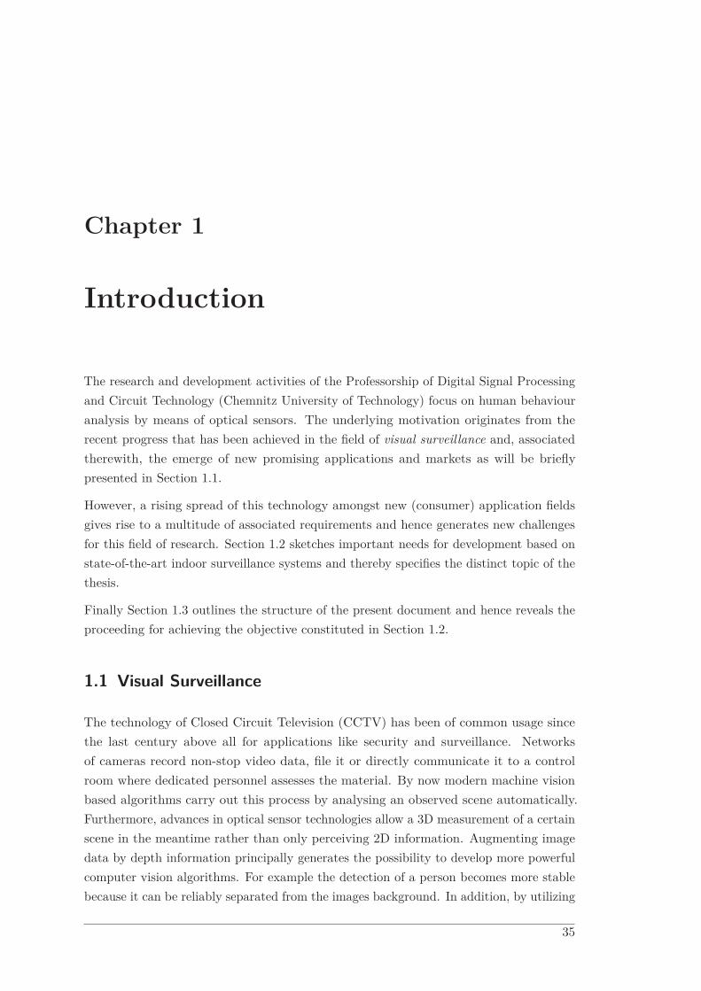
The research and development activities of the Professorship of Digital Signal Processingand Circuit Technology (Chemnitz University of Technology) focus on human behaviouranalysis by means of optical sensors. The underlying motivation originates from therecent progress that has been achieved in the field of visual surveillance and, associatedtherewith, the emerge of new promising applications and markets as will be brieflypresented in Section 1.1.
However, a rising spread of this technology amongst new (consumer) application fieldsgives rise to a multitude of associated requirements and hence generates new challengesfor this field of research. Section 1.2 sketches important needs for development based onstate-of-the-art indoor surveillance systems and thereby specifies the distinct topic of thethesis.
Finally Section 1.3 outlines the structure of the present document and hence reveals theproceeding for achieving the objective constituted in Section 1.2.
1.1 Visual Surveillance
The technology of Closed Circuit Television (CCTV) has been of common usage sincethe last century above all for applications like security and surveillance. Networksof cameras record non-stop video data, file it or directly communicate it to a controlroom where dedicated personnel assesses the material. By now modern machine visionbased algorithms carry out this process by analysing an observed scene automatically.Furthermore, advances in optical sensor technologies allow a 3D measurement of a certainscene in the meantime rather than only perceiving 2D information. Augmenting imagedata by depth information principally generates the possibility to develop more powerfulcomputer vision algorithms. For example the detection of a person becomes more stablebecause it can be reliably separated from the images background. In addition, by utilizing
35
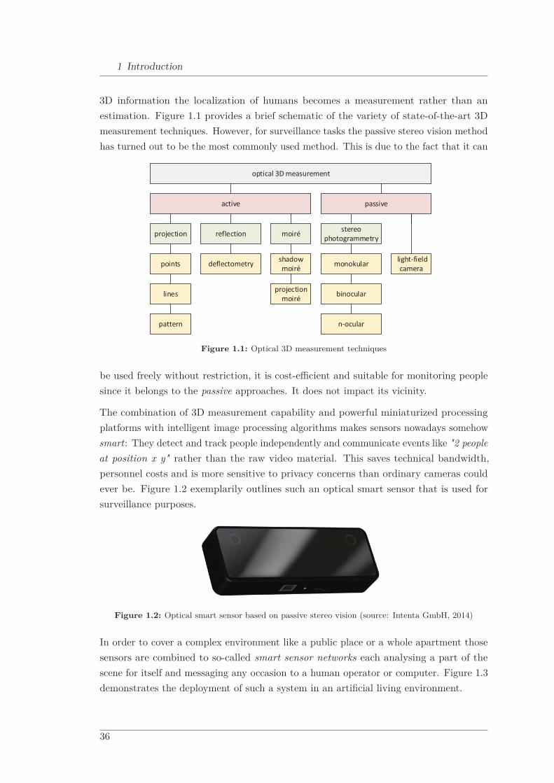
1 Introduction
3D information the localization of humans becomes a measurement rather than anestimation. Figure 1.1 provides a brief schematic of the variety of state-of-the-art 3Dmeasurement techniques. However, for surveillance tasks the passive stereo vision methodhas turned out to be the most commonly used method. This is due to the fact that it can
optical 3D measurement
active passive
projection
deflectometry
reflection moiré
points
lines
pattern
shadow moiré
projection moiré
stereophotogrammetry
monokular
binocular
n-ocular
light-field camera
Figure 1.1: Optical 3D measurement techniques
be used freely without restriction, it is cost-efficient and suitable for monitoring peoplesince it belongs to the passive approaches. It does not impact its vicinity.
The combination of 3D measurement capability and powerful miniaturized processingplatforms with intelligent image processing algorithms makes sensors nowadays somehowsmart: They detect and track people independently and communicate events like "2 peopleat position x y" rather than the raw video material. This saves technical bandwidth,personnel costs and is more sensitive to privacy concerns than ordinary cameras couldever be. Figure 1.2 exemplarily outlines such an optical smart sensor that is used forsurveillance purposes.
Figure 1.2: Optical smart sensor based on passive stereo vision (source: Intenta GmbH, 2014)
In order to cover a complex environment like a public place or a whole apartment thosesensors are combined to so-called smart sensor networks each analysing a part of thescene for itself and messaging any occasion to a human operator or computer. Figure 1.3demonstrates the deployment of such a system in an artificial living environment.
36

1.1 Visual Surveillance
Figure 1.3: Apartment equipped with a smart sensor network
For example the new upcoming Ambient Assisted Living (AAL) market claims safetyand assistance functionality for elderly people that live at home alone. A smart sensorbased system can provide functionalities like fall detection, emergency alerting and homeautomation services while paying attention to the inhabitants privacy concerns. Figure 1.4shows a scenario where an elderly person that has fallen on the floor is guarded by anoptical sensor system.
Figure 1.4: Emergency detection in a domestic environment (source: Vitracom AG, 2015)
A few more examples for relevant markets shall be stated in Table 1.1.
37

1 Introduction
Table 1.1: Markets and application fields
Market Explanation Exemplary Applications
AAL Age-based homes equipped withsmart sensors take care of the el-derly inhabitants and assist withtheir everyday live.
Fall detection, emergency alerting,home automation services, assis-tance for carrying out ADLs, careoptimization by evaluation of sta-tistical data of the inhabitants be-haviour and health status
Security Private homes as well as publicbuildings are equipped with intel-ligent sensors that message suspi-cious or violent behaviour.
Intrusion detection, access control,crowd density monitoring aban-doned object detection, theft de-tection
BuildingAutomation
Smart sensors detect and count peo-ple to make buildings somehow in-telligent by automatically perform-ing certain services.
Air conditioning control, accesscontrol, energy management, HMIfor established building automationsystems e.g. of Honeywell Interna-tional Inc.
Retail Smart sensor systems for retail busi-ness intelligence collect data aboutthe number of customers and theirpurchasing behaviour.
Managing queues of customers atcash boxes, analysing the shop per-formance
Industry Perspectively, manual manufactur-ing processes will be guided by au-tomatic systems that take care ofproduction policies, safety and lo-gistical concerns.
Safety in production by intrusionor tiredness detection, process mon-itoring
1.2 Challenges in Visual Surveillance
Reviewing state-of-the art visual surveillance technology and its markets, the systemcosts turn out to be an everlasting crucial issue. One of the key cost drivers is the numberof applied sensors for observing a certain scene. Hence, it is obvious that a reduction ofnecessary sensors (and the attached infrastructure) can have an essential impact on thesystems price.
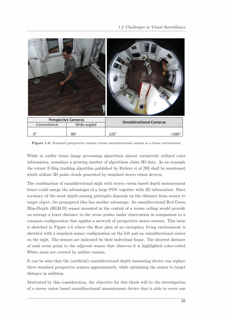
Complex scenes as for example a living environment usually require 2 to 3 ordinaryperspective sensors per room for almost full coverage. Due to their nature of perspectiveprojection they are restricted to a Field of View (FOV) of much less than 180o. Specialdevices called omnidirectional sensors work either with catadioptric mirror configurationsor are equipped with fish-eye lenses in order to generate a FOV of more than 180o.Figure 1.5 shows an exemplary living environment observed by a perspective, and forcomparison, an omnidirectional imaging device. The latter generates a much largervisible area and is hence appropriate to replace multiple perspective sensors.
38
1.2 Challenges in Visual Surveillance
Perspective Cameras Omnidirectional CamerasConventional Wide-angled
0° 80° 120° >180°
Figure 1.5: Standard perspective camera versus omnidirectional camera in a home environment
While in earlier times image processing algorithms almost exclusively utilized colorinformation, nowadays a growing number of algorithms claim 3D data. As an examplethe robust Z-Map tracking algorithm published by Richter et al [99] shall be mentioned,which utilizes 3D point clouds generated by standard stereo vision devices.
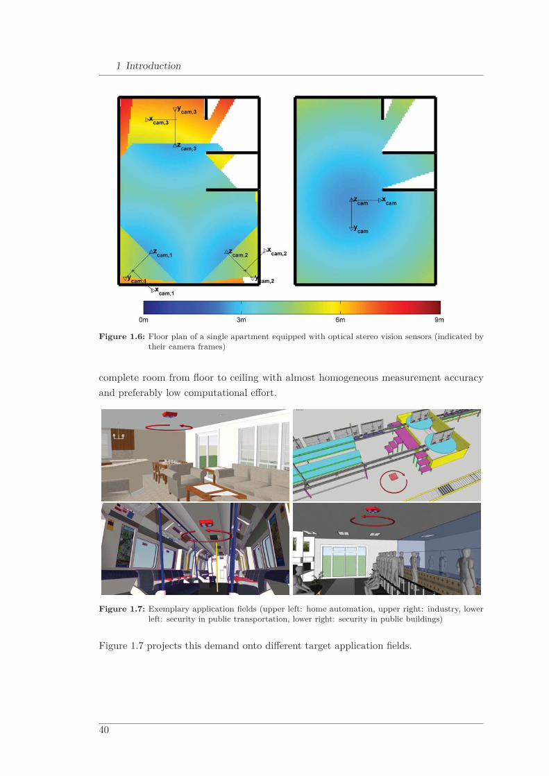
The combination of omnidirectional sight with stereo vision based depth measurementhence could merge the advantages of a large FOV together with 3D information. Sinceaccuracy of the most depth sensing principles depends on the distance from sensor totarget object, the propagated idea has another advantage: An omnidirectional Red GreenBlue-Depth (RGB-D) sensor mounted in the central of a rooms ceiling would provideon average a lower distance to the scene points under observation in comparison to acommon configuration that applies a network of perspective stereo sensors. This issueis sketched in Figure 1.6 where the floor plan of an exemplary living environment issketched with a standard sensor configuration on the left and an omnidirectional sensoron the right. The sensors are indicated by their individual frame. The shortest distanceof each scene point to the adjacent sensor that observes it is highlighted color-coded.White areas are covered by neither camera.
It can be seen that the (artificial) omnidirectional depth measuring device can replacethree standard perspective sensors approximately, while optimizing the sensor to targetdistance in addition.
Motivated by this consideration, the objective for this thesis will be the investigationof a stereo vision based omnidirectional measurement device that is able to cover one
39
1 Introduction
Figure 1.6: Floor plan of a single apartment equipped with optical stereo vision sensors (indicated bytheir camera frames)
complete room from floor to ceiling with almost homogeneous measurement accuracyand preferably low computational effort.
Figure 1.7: Exemplary application fields (upper left: home automation, upper right: industry, lowerleft: security in public transportation, lower right: security in public buildings)
Figure 1.7 projects this demand onto different target application fields.
40

1.3 Outline of the Thesis
1.3 Outline of the Thesis
The present script is organized as follows:
Chapter 2 - Fundamentals of Computer Vision Geometry
As a starting point relevant basics of computer vision are structured and elaborated forcertain aspects that are important for this work. This is done in Chapter 2.
Chapter 3 - Fundamentals of Stereo Vision
Stereo vision fundamentals for standard perspective camera geometry are presentedsuccessively in Chapter 3. This technology plays a key role in this work and will betransferred to other camera models subsequently.
Chapter 4 - Virtual Perspective Cameras
For the simultaneous usage of different camera models and their conversion, it is importantto understand the concept of virtual cameras. In Chapter 4 several conversion strategiesfrom omnidirectional to perspective vision are investigated exemplarily.
Chapter 5 - Spherical Stereo Vision
The research field of stereo vision with respect to multiple omnidirectional geometries isrevised in Chapter 5. Different approaches are compared and assessed with respect tothe application of visual surveillance.
Chapter 6 - A Novel Spherical Stereo Vision Algorithm
Based on the knowledge presented in Chapter 2, Chapter 3, Chapter 4 and Chapter 5 a newmethod for omnidirectional stereo processing is presented and simulated in Chapter 6.
Chapter 7 - Spherical Stereo Vision Demonstrator
A real demonstrator compiled of standard industry cameras is presented in Chapter 7.
Chapter 8 - Discussion and Outlook
Finally, in Chapter 8 the so far achieved results of this thesis are discussed and open pointscollected. In addition, possible improvements for the presented concept are suggested.A sample application that employs omnidirectional RGB-D data concludes this thesispractically.
41


Chapter 2
Fundamentals of Computer VisionGeometry
This chapter discusses fundamental topics related to computer vision geometry. As start-ing point vital basics for homogeneous and inhomogeneous coordinate representations arebriefly reviewed in Section 2.1. After this the principles of transferring a 3D point locatedin an observed scene to a 2D image point is treated in Section 2.2 while distinguishingdifferent camera models. Subsequently a brief overview of current state-of-the-art meth-ods for estimating the parameters of different camera models for the usage in real cameradevices is presented in Section 2.3. Finally an insight into the fundamental mechanics ofepipolar geometry is given in Section 2.4. The constraints that two adjacent camerasintroduce on the relationships between their images are explained.
2.1 Projective Geometry
In the following sections the most important geometrical point representations for two- andthree-dimensional space are explained - more precisely homogeneous and inhomogeneousrepresentations.
2.1.1 Euclidean Space
The most common form of representing a point is the expression of cartesian coordinates.Let X2D and X3D be points in 2D and 3D space, than one can represent them as shown
43
2 Fundamentals of Computer Vision Geometry
in Equation 2.1
X2D =
⎛⎝x
y
⎞⎠ , X3D =
⎛⎜⎜⎜⎝x
y
z
⎞⎟⎟⎟⎠ (2.1)
where x, y and z are the vector components in the direction of the x-, y- and z-axis,respectively. This model is commonly used in the euclidean space. Different scalar valuesof the components represent different points.
2.1.2 Projective Space
In the projective space the distinct values of the vectors components are not significantfor determining a unique point, but so are the ratios between the values. For example inthis space a point X1 = (1,2,3)T is equivalent to a point X2 = (2,4,6)T , since both headfor the same direction. Although a point X3 = (∞,∞,∞)T resides at infinity it can beequivalent to X1 and X2 as well if their direction is identical.
In order to represent finite and infinite points homogeneously, the homogeneous repre-sentation was introduced, by adding an additional scale factor w. This new parameterencodes the scale of the vector while the others represent its direction. ConsequentlyX2D and X3D are now given as 3- and 4-dimensional vectors in 2- and 3-dimensionalspace and are called the homogeneous representation:
X2D =
⎛⎜⎜⎜⎝x
y
w
⎞⎟⎟⎟⎠ , X3D =
⎛⎜⎜⎜⎜⎜⎜⎝x
y
z
w
⎞⎟⎟⎟⎟⎟⎟⎠ (2.2)
The inhomogeneous representation (without w) is marked in the following with a tilde asX2D and X3D:
X2D =
⎛⎝x/w
y/w
⎞⎠ , X3D =
⎛⎜⎜⎜⎝x/w
y/w
z/w
⎞⎟⎟⎟⎠ (2.3)
The afore-mentioned example points have the following homogeneous and inhomogeneousrepresentations:
X1 = (1,2,3,1)T → X1 = (1,2,3)T
X2 = (1,2,3,0.5)T → X2 = (2,4,6)T
X3 = (1,2,3,0)T → X3 = (∞,∞,∞)T
(2.4)
44
2.2 Camera Geometry
From now on the distinction between both models is made.
2.2 Camera Geometry
A camera usually maps an observed 3D scene to a 2D image. The geometrical relationshipbetween these 3D scene points X3D and the resulting 2D image points X2D is oftenquite complex due to the physical construction of the imaging device.
This complex issue can be approximated by an appropriate mathematical model which iscommonly known as camera model or projection model. By employing a finite amount ofnumerical parameters, the actual process of projection can be replaced by an appropriatemathematical relationship of bearable computational cost.
Since the original scene points refer to a certain 3D world coordinate system, they arefrom now on called Xwrld. Since the target 2D points refer to an image coordinatesystem, they are from now on called X img:
Xwrld =
⎛⎜⎜⎜⎜⎜⎜⎝xwrld
ywrld
zwrld
wwrld
⎞⎟⎟⎟⎟⎟⎟⎠ , X img =
⎛⎜⎜⎜⎝ximg
yimg
wimg
⎞⎟⎟⎟⎠ (2.5)
2.2.1 Geometrical Imaging Process
The overall imaging process that transfers a scene point Xwrld to an image point X img
successively utilizes an extrinsic and an intrinsic model as can be seen in Figure 2.1:
• The former describes the geometrical relationship of a global reference, the WorldCoordinate System (WCS), with respect to the camera itself, the camera coordinatesystem. It considers Xwrld with respect to a world reference as a world point andtransfers it to a camera point Xcam. See Section 2.2.1.2.
• The latter describes the projection process from camera points Xcam to imagepoints X img in the image coordinate system. See Section 2.2.1.1.
45

2 Fundamentals of Computer Vision Geometry
Figure 2.1: Coordinate transformations in the geometrical imaging process
2.2.1.1 Projection Models
The projection model describes the mapping from incoming light rays, denoted by Xcam,to normalized sensor coordinates, denoted by Xnorm, whereby
Xcam =
⎛⎜⎜⎜⎜⎜⎜⎝xcam
ycam
zcam
wcam
⎞⎟⎟⎟⎟⎟⎟⎠ and Xnorm =
⎛⎜⎜⎜⎝xnorm
ynorm
1
⎞⎟⎟⎟⎠ (2.6)
are the corresponding homogeneous Cartesian representations in camera and normalizedsensor coordinate system respectively.
A special group of projection principles are so called radially symmetric models. Thereforeit may be suitable to note the spherical and the polar representation respectively:
Xcam =
⎛⎜⎜⎜⎝θ
ϕ
wcam
⎞⎟⎟⎟⎠ and Xnorm =
⎛⎜⎜⎜⎝ρ
ϕ
1
⎞⎟⎟⎟⎠ (2.7)
The following conventions apply for these mathematical expressions:
• The variable θ is the angle between the incoming light ray and the optical axis.
• The variable ϕ forms the azimuth angle of the incoming light ray.
• The variable ρ forms the radius of the projected normalized sensor point withrespect to the centre of the image.
46

2.2 Camera Geometry
In Figure 2.2 the relationship of the coordinates of Xcam before and of Xnorm after theprojection by a radially symmetric model can be seen.
Figure 2.2: Projection process
According to [56] the radial projection of an incoming light ray Φ = (θ,ϕ)T onto a virtualimage plane with a distance of f = 1 to the projection center can be modelled with theradial projection function
Xnorm = F (Φ) = ρ(θ)ur(ϕ) with ur(ϕ) =
⎛⎝cosϕ
sinϕ
⎞⎠ (2.8)
where ρ(θ) is the projection radius as a function of θ and ur is the unit vector in radialdirection.
In Table 2.1 a variety of the most important radially symmetric projection models aresummarized as presented in [56]. Asymmetric effects of projection are not covered bythose models.
In Figure 2.3 the projection principles of Table 2.1 are visualized.
For projection principles called non-radially symmetric models it is more appropriate tomodel the projection by employing Cartesian coordinates:
Xnorm = F(Xcam
)(2.14)
2.2.1.2 Intrinsic Model
Modern cameras employ a discrete number of sensor or picture elements on the lightsensitive chip. Image information is thereby described by image or pixel coordinates
47
2 Fundamentals of Computer Vision Geometry
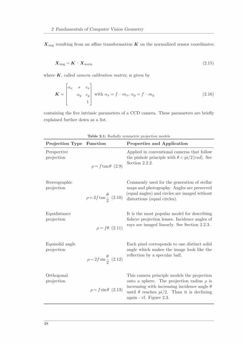
X img resulting from an affine transformation K on the normalized sensor coordinates:
X img = K ·Xnorm (2.15)
where K, called camera calibration matrix, is given by
K =
⎡⎢⎢⎢⎣αx s cx
αy cy
1
⎤⎥⎥⎥⎦ with αx = f ·mx, αy = f ·my (2.16)
containing the five intrinsic parameters of a CCD camera. These parameters are brieflyexplained further down as a list.
Table 2.1: Radially symmetric projection models
Projection Type Function Properties and Application
Perspectiveprojection
ρ = f tanθ (2.9)
Applied in conventional cameras that followthe pinhole principle with θ < pi/2 [rad]. SeeSection 2.2.2.
Stereographicprojection
ρ = 2f tanθ
2(2.10)
Commonly used for the generation of stellarmaps and photography. Angles are preserved(equal angles) and circles are imaged withoutdistortions (equal circles).
Equidistanceprojection
ρ = fθ (2.11)
It is the most popular model for describingfisheye projection lenses. Incidence angles ofrays are imaged linearly. See Section 2.2.3.
Equisolid angleprojection
ρ = 2f sinθ
2(2.12)
Each pixel corresponds to one distinct solidangle which makes the image look like thereflection by a specular ball.
Orthogonalprojection
ρ = f sinθ (2.13)
This camera principle models the projectiononto a sphere. The projection radius ρ isincreasing with increasing incidence angle θuntil θ reaches pi/2. Than it is decliningagain - cf. Figure 2.3.
48

2.2 Camera Geometry
Figure 2.3: Radially symmetric projections
• αx is the focal length f normalized to the physical horizontal pixel length px.[αx] = px
mm . The inverse of px is called horizontal pixel density mx. [mx] = 1mm
• αy is the focal length f normalized to the physical vertical pixel length py. [αy] = pxmm .
The inverse of py is called vertical pixel density my. [my] = 1mm
• cx is the horizontal offset value of the principle point from the pixel frame. [cx] = px.
• cy is the vertical offset value of the principle point from the pixel frame. [cy] = px.
• s is the affine distortion of the image in horizontal direction, called skewness factor.[s] = mm·rad.
For an ideal camera the offset values cx and cy can be directly exploited to calculate theimage size {height,width}. The relationship is outlined in Equation 2.17.
{cx, cy} = {width +12
,height+1
2} (2.17)
49

2 Fundamentals of Computer Vision Geometry
2.2.1.3 Extrinsic Model
Generally the scene point is expressed in a world coordinate system Xwrld which isdifferent from the camera coordinate system and which is useful especially when thereare multiple cameras in the scene - see Figure 2.4. The geometrical relationship between
Figure 2.4: World coordinate system
Xwrld the coordinate systems Xcam,i (with i being the index of the distinct camera)is composed of a 3 × 3 rotation matrix Ri and a 3 × 1 translation vector T i. A pointgiven in world coordinates can hence be transferred into camera coordinates by applyingEquation 2.18:
Xcam,i = Ri ·Xwrld +T i (2.18)
Using homogeneous coordinates, this procedure can be expressed as matrix operation:
Xcam,i = H i ·Xwrld (2.19)
where H i denotes the 4×4 homography matrix describing the world coordinate systemwith respect to the camera coordinate system. H i can be decomposed as follows:
H i =
⎡⎣Ri T i
0 1
⎤⎦ =
⎡⎣Ri −RiC i
0 1
⎤⎦ (2.20)
where C i is a 3×1 vector which encodes the position of the camera in world coordinates.
50

2.2 Camera Geometry
Furthermore R can be decomposed into the angles ϕx, ϕy and ϕz. They represent therotation of the camera with respect to the WCS as a consecutive turn of the cameraaround its own x-, y- and z-axis respectively. These angles are called Euler rotations.
2.2.1.4 Distortion Models
Every projection model has the limitation that it approximates real Commercial Off-The-Shelf (COTS) cameras at its best due to manufacturing issues. Furthermore evenlenses of the same type differ in their imaging behaviour. These properties are denotedas distortions. It is commonly distinguished between:
• Radial distortions: Especially wide-angle lenses of cheap production commonlygive rise to deviations of the projection result from the invoked model in radialdirection.
• Tangential distortions: Especially skew assembling of the lens and die in acamera lead to tangential deviations of the projection result.
There are several approaches available to extend the camera models with a description ofthese lens imperfections. See Section 2.2.2 and Section 2.2.4.
2.2.2 Pinhole Camera Model
Most conventional cameras which follow the perspective camera model use the pinholecamera model as an approximation. Essentially it is a perspective projection of thespatial coordinates Xcam given in the camera coordinate system denoted by
Xcam =
⎛⎜⎜⎜⎜⎜⎜⎝xcam
ycam
zcam
1
⎞⎟⎟⎟⎟⎟⎟⎠ (2.21)
into normalized sensor plane coordinates Xnorm
Xnorm =
⎛⎜⎜⎜⎝xnorm
ynorm
1
⎞⎟⎟⎟⎠ =1
zcam
⎛⎜⎜⎜⎝f ·xcam
f ·ycam
zcam
⎞⎟⎟⎟⎠ =1
zcam
⎡⎢⎢⎢⎣f 0
f 01 0
⎤⎥⎥⎥⎦Xcam (2.22)
51

2 Fundamentals of Computer Vision Geometry
Figure 2.5: Perspective camera model
whereby f forms the focal length of the camera and hence the distance between theprincipal point and the sensor plane of the camera. In Figure 2.5 the camera modelpresented so far is visualized.
Similarly a radially symmetric projection function Fp can describe the projection processby combining Equation 2.8 with Equation 2.9:
Xnorm = Fp (Φ) = f tanθ
⎛⎝cosϕ
sinϕ
⎞⎠ =(
fxcam
zcam,f
ycam
zcam
)T
(2.23)
2.2.2.1 Complete Forward Model
Perspective projection modelIntegrating all the previous relations, a 3D point Xwrld can be directly transferred intoimage coordinates by setting up a 3×4 camera projection matrix P :
X img = P ·Xwrld (2.24)
This matrix is composed of the intrinsic parameters K as well as extrinsic parameters R
and T :
P = K[R T
](2.25)
Altogether this model provides 11 Degrees of Freedom (DOF) for modelling a perspectivecamera.
52

2.2 Camera Geometry
In a mathematical sense, the matrix P is the projection of a four dimensional space (3Dhomogeneous points) to a three dimensional space (2D homogeneous points). Amongstother possibilities, P (with the 12 scalar elements p11 to p34) can be represented as
• a column vector of components p1R, p2R and p3R where each element is a 1 × 4row vector.
• a row vector of components p1C, p2C, p3C and p4C where each element is a 3×1column vector.
This relationship is highlighted in Equation 2.26.
P =
⎡⎢⎢⎢⎣p11 p12 p13 p14
p21 p22 p23 p24
p31 p32 p33 p34
⎤⎥⎥⎥⎦ =
⎡⎢⎢⎢⎣p1R
p2R
p3R
⎤⎥⎥⎥⎦ =[p1C p2C p3C p4C
](2.26)
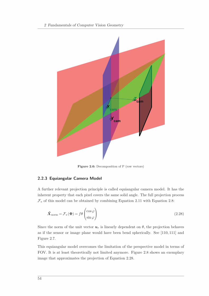
Decomposing P into row vectors means to represent it by a number of special planes:
• p1R is the plane orthogonal to the camera’s x-axis containing the principal pointand origin of the image coordinate system. It is visualized in Figure 2.6 as redplane.
• p2R is the plane orthogonal to the camera’s y-axis containing the principal pointand origin of the image coordinate system. It is visualized in Figure 2.6 as greenplane.
• p3R is the principal plane. It is visualized in Figure 2.6 as blue plane.
Decomposing P into column vectors means to represent it by a number of special points:
• p1C, p2C and p3C are the projections of the x-, y- and z-axis directions of the worldframe.
• p4C is the projection of the origin of the world frame.
2.2.2.2 Back Projection
The operation of projecting a 3D point Xwrld to an image point X img (see Equation 2.24)is not reversible since P is not invertible. In other words, a 2D image point cannot beused to recover a 3D world point. Rather than this, it can be used to recover a ray ofpoints by employing the pseudo inverse of P , denoted by P +:
Xwrld (λ) = λ·P +X img +C with P + = P T(P P T
)−1(2.27)
At this point λ represents an arbitrary scale factor and hence the uncertainty of theworld point recovery.
53
2 Fundamentals of Computer Vision Geometry
Figure 2.6: Decomposition of P (row vectors)
2.2.3 Equiangular Camera Model
A further relevant projection principle is called equiangular camera model. It has theinherent property that each pixel covers the same solid angle. The full projection processFe of this model can be obtained by combining Equation 2.11 with Equation 2.8:
Xnorm = Fe (Φ) = fθ
⎛⎝cosϕ
sinϕ
⎞⎠ (2.28)
Since the norm of the unit vector ur is linearly dependent on θ, the projection behavesas if the sensor or image plane would have been bend spherically. See [110, 111] andFigure 2.7.
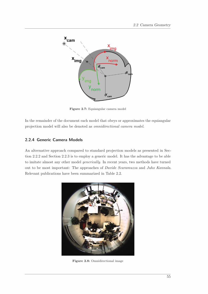
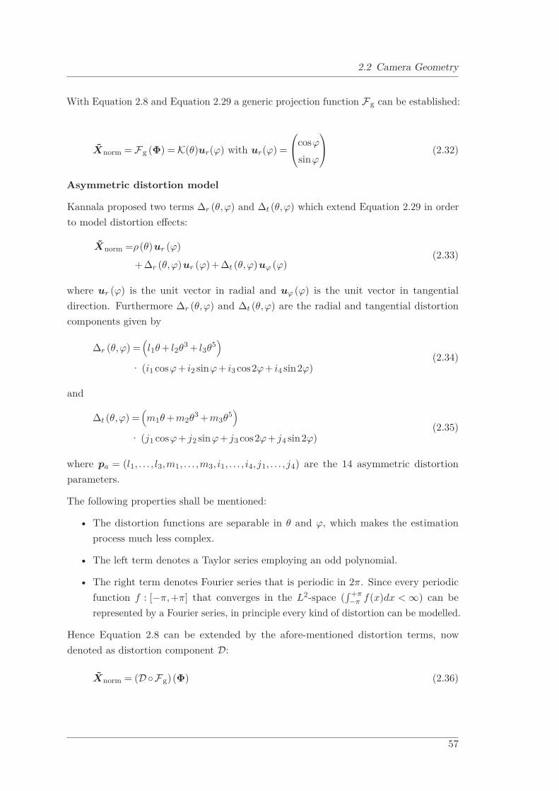
This equiangular model overcomes the limitation of the perspective model in terms ofFOV. It is at least theoretically not limited anymore. Figure 2.8 shows an exemplaryimage that approximates the projection of Equation 2.28.
54
2.2 Camera Geometry
Figure 2.7: Equiangular camera model
In the remainder of the document each model that obeys or approximates the equiangularprojection model will also be denoted as omnidirectional camera model.
2.2.4 Generic Camera Models
An alternative approach compared to standard projection models as presented in Sec-tion 2.2.2 and Section 2.2.3 is to employ a generic model. It has the advantage to be ableto imitate almost any other model generically. In recent years, two methods have turnedout to be most important: The approaches of Davide Scaramuzza and Juho Kannala.Relevant publications have been summarized in Table 2.2.
Figure 2.8: Omnidirectional image
55

2 Fundamentals of Computer Vision Geometry
Table 2.2: Generic projection models
Projection Model Properties and Application Publications
Kannala’s Camera Model Describes a variety of common aswell as omnidirectional cameratypes. Claims to sufficiently ap-proximate all types of Table 2.1.
[53, 55–57]
Scaramuzza’s Camera Model Describes a variety of commonas well as omnidirectional cam-era types. It puts emphasis oncatadioptric imaging systems.
[102–104]
The model proposed by Juho Kannala shall be examined here in more detail, whilethe method of Davide Scaramuzza has been mentioned as an alternative way. In [56]Juho Kannala describes his method to comprise three components: a radially symmet-ric projection model, an asymmetric distortion model and a transformation to imagecoordinates.
Together these components describe the so called complete forward model to transfer a3D point Xcam into an image point X img. The inverse way is called back projection - cf.Section 2.2.1.1 and Section 2.2.1.2. In the following both are outlined briefly.
2.2.4.1 Complete Forward Model
Radial symmetric projection model
The radial symmetric model proposed by [56] describes the projection (Section 2.2.1) ina general polynomial form
ρ(θ) = K(θ) = k1θ +k2θ3 +k3θ5 +k4θ7 +k4θ9 + . . . (2.29)
where the even powers are neglectable, as the projection is radially symmetric related to theprojection center. By parametrizing the polynomial appropriately, all common projectiontypes can be approximated sufficiently. According to [56] the first five coefficients aresufficient. Exemplarily the Taylor series of the pinhole camera model with ρ(θ) = tanθ,and hence its approximation can be parametrized as follows:
ρ(θ) = θ +13
θ3 +215
θ5 +17315
θ7 +62
2835θ9 +R(θ) (2.30)
with R(θ) being the residuum. For the perfect equiangular projection it reduces just to
ρ(θ) = θ (2.31)
56
2.2 Camera Geometry
With Equation 2.8 and Equation 2.29 a generic projection function Fg can be established:
Xnorm = Fg (Φ) = K(θ)ur(ϕ) with ur(ϕ) =
⎛⎝cosϕ
sinϕ
⎞⎠ (2.32)
Asymmetric distortion model
Kannala proposed two terms Δr (θ,ϕ) and Δt (θ,ϕ) which extend Equation 2.29 in orderto model distortion effects:
Xnorm =ρ(θ)ur (ϕ)
+Δr (θ,ϕ)ur (ϕ)+Δt (θ,ϕ)uϕ (ϕ)(2.33)
where ur (ϕ) is the unit vector in radial and uϕ (ϕ) is the unit vector in tangentialdirection. Furthermore Δr (θ,ϕ) and Δt (θ,ϕ) are the radial and tangential distortioncomponents given by
Δr (θ,ϕ) =(l1θ + l2θ3 + l3θ5
)· (i1 cosϕ+ i2 sinϕ+ i3 cos2ϕ+ i4 sin2ϕ)
(2.34)
and
Δt (θ,ϕ) =(m1θ +m2θ3 +m3θ5
)· (j1 cosϕ+ j2 sinϕ+ j3 cos2ϕ+ j4 sin2ϕ)
(2.35)
where pa = (l1, . . . , l3,m1, . . . ,m3, i1, . . . , i4, j1, . . . , j4) are the 14 asymmetric distortionparameters.
The following properties shall be mentioned:
• The distortion functions are separable in θ and ϕ, which makes the estimationprocess much less complex.
• The left term denotes a Taylor series employing an odd polynomial.
• The right term denotes Fourier series that is periodic in 2π. Since every periodicfunction f : [−π,+π] that converges in the L2-space (
∫ +π−π f(x)dx < ∞) can be
represented by a Fourier series, in principle every kind of distortion can be modelled.
Hence Equation 2.8 can be extended by the afore-mentioned distortion terms, nowdenoted as distortion component D:
Xnorm = (D ◦Fg)(Φ) (2.36)
57
2 Fundamentals of Computer Vision Geometry
Transformation to image coordinates
To finally transfer normalized sensor coordinates into image coordinates, a further affinetransformation A is applied in accordance with Section 2.2.1.2:
X img =
⎛⎝ximg
yimg
⎞⎠ = A(Xnorm
)=
⎡⎣αx 00 αy
⎤⎦Xnorm +
⎛⎝cx
cy
⎞⎠ (2.37)
Complete forward model
Altogether the camera model defined above contains 23 camera parameters. Thereforeit is denoted by p23. Leaving out the asymmetric part it is reduced to p9. Using onlytwo instead of five parameters for the radial component we obtain p6. The resultingparameter vectors are given by
p6 = (k1,k2,αx,αy, cx, cy)T
p9 = (k1,k2,αx,αy, cx, cy,k3,k4,k5)T
p23 = (k1,k2,αx,αy, cx, cy,k3,k4,k5, l1...l3, i1...i4, j1...j4)T
(2.38)
Summarizing all the operations, the whole forward camera model P (Φ) can be denotedas:
X img = P (Φ) = (A◦D ◦Fg)(Φ) (2.39)
2.2.4.2 Back Projection
Back projection is the process of recovering a ray Xcam parametrized by Φ (comparewith Equation 2.7 and Equation 2.8) from an image point X img.
Xcam = Φ =(F−1
g ◦D−1 ◦A−1)
X img (2.40)
2.3 Camera Calibration Methods
Since each projection model that shall be applied needs to be parametrized appropriately,in the following common methods for the process denoted as camera calibration will bepresented at a glance. Provided that, the physical projection can be roughly reproducedby an ideal mathematical model as seen in Section 2.2, at this stage the estimation of allparameters of the distinct model is within the focus.
58
2.3 Camera Calibration Methods
Since there exist a vast range of approaches for calibration in literature for not less thana multitude of camera models, this section can merely provide a brief overview of themost important procedures for the pinhole camera model and the omnidirectional cameramodel. A more detailed illustration can be found in [79].
2.3.1 Perspective Camera Calibration
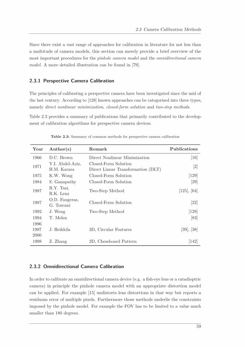
The principles of calibrating a perspective camera have been investigated since the mid ofthe last century. According to [128] known approaches can be categorized into three types,namely direct nonlinear minimization, closed-form solution and two-step methods.
Table 2.3 provides a summary of publications that primarily contributed to the develop-ment of calibration algorithms for perspective camera devices.
Table 2.3: Summary of common methods for perspective camera calibration
Year Author(s) Remark Publications
1966 D.C. Brown Direct Nonlinear Minimization [16]
1971 Y.I. Abdel-Aziz,H.M. Karara
Closed-Form SolutionDirect Linear Transformation (DLT) [2]
1975 K.W. Wong Closed-Form Solution [129]1984 S. Ganapathy Closed-Form Solution [29]
1987 R.Y. Tsai,R.K. Lenz Two-Step Method [125], [64]
1987 O.D. Faugeras,G. Toscani Closed-Form Solution [22]
1992 J. Weng Two-Step Method [128]1994 T. Melen [83]199619972000
J. Heikkila 3D, Circular Features [39], [38]
1998 Z. Zhang 2D, Chessboard Pattern [142]
2.3.2 Omnidirectional Camera Calibration
In order to calibrate an omnidirectional camera device (e.g. a fish-eye lens or a catadioptriccamera) in principle the pinhole camera model with an appropriate distortion modelcan be applied. For example [15] undistorts lens distortions in that way but reports aresiduum error of multiple pixels. Furthermore those methods underlie the constraintsimposed by the pinhole model. For example the FOV has to be limited to a value muchsmaller than 180 degrees.
59
2 Fundamentals of Computer Vision Geometry
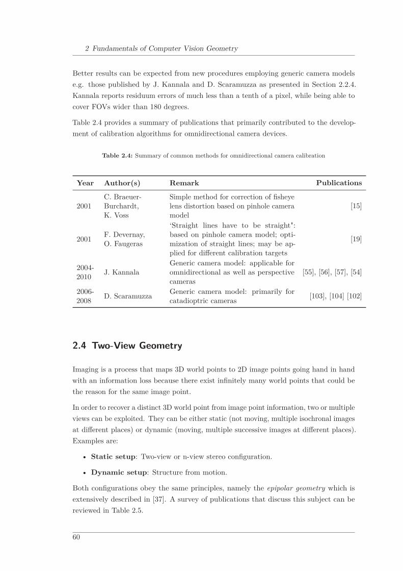
Better results can be expected from new procedures employing generic camera modelse.g. those published by J. Kannala and D. Scaramuzza as presented in Section 2.2.4.Kannala reports residuum errors of much less than a tenth of a pixel, while being able tocover FOVs wider than 180 degrees.
Table 2.4 provides a summary of publications that primarily contributed to the develop-ment of calibration algorithms for omnidirectional camera devices.
Table 2.4: Summary of common methods for omnidirectional camera calibration
Year Author(s) Remark Publications
2001C. Braeuer-Burchardt,K. Voss
Simple method for correction of fisheyelens distortion based on pinhole cameramodel
[15]
2001 F. Devernay,O. Faugeras
‘Straight lines have to be straight":based on pinhole camera model; opti-mization of straight lines; may be ap-plied for different calibration targets
[19]
2004-2010 J. Kannala
Generic camera model: applicable foromnidirectional as well as perspectivecameras
[55], [56], [57], [54]
2006-2008 D. Scaramuzza Generic camera model: primarily for
catadioptric cameras [103], [104] [102]
2.4 Two-View Geometry
Imaging is a process that maps 3D world points to 2D image points going hand in handwith an information loss because there exist infinitely many world points that could bethe reason for the same image point.
In order to recover a distinct 3D world point from image point information, two or multipleviews can be exploited. They can be either static (not moving, multiple isochronal imagesat different places) or dynamic (moving, multiple successive images at different places).Examples are:
• Static setup: Two-view or n-view stereo configuration.
• Dynamic setup: Structure from motion.
Both configurations obey the same principles, namely the epipolar geometry which isextensively described in [37]. A survey of publications that discuss this subject can bereviewed in Table 2.5.
60

2.4 Two-View Geometry
For simplification, further explanations with respect to epipolar geometry in Section 2.4.1and Section 2.4.2 refer to the ideal pinhole camera model from Section 2.2.2. SubsequentlySection 2.4.3 generalizes certain aspects to omnidirectional imaging devices.
Table 2.5: Summary of publications that treat common two-view geometry
Year Author(s) Remark Publications
1987 H. C. Longuet-Higgins
A computer algorithm for reconstruct-ing a scene from two projections [72]
1993 Faugeras, OliverD.
Three dimensional computer vision: Ageometric viewpoint [21]
1996
Luong, Quan-TuanandFaugeras, OlivierD
The fundamental matrix: Theory, algo-rithms, and stability analysis [75]
1997
Gabriella Csurkaand Cyril Zellerand ZhengyouZhang andOlivier D.Faugeras
Characterizing the Uncertainty of theFundamental Matrix [18]
1998 Zhang, Zhengyou Determining the epipolar geometry andits uncertainty: A review [141]
1999Gang Xuand ZhengyouZhang
Epipolar Geometry in Stereo, Motionand Object Recognition [131]
2000,2003
Hartley, Richardand Zisserman,Andrew
Multiple view geometry in computervision [36,37]
2.4.1 Epipolar Geometry
We consider two views in arbitrary geometrical configuration as can be seen in Figure 2.9.Both views are individually described by projection matrices P l (left) and P r (right).However, their mutual geometrical relationship can be described by epipolar geometry.While the structure of the observed scene itself does not influence this geometry, itdepends on the camera’s intrinsics and relative extrinsics. In Figure 2.9 a 3D world pointXwrld projects to the image points X img,l and X img,r.
Important properties of this configuration are:
61

2 Fundamentals of Computer Vision Geometry
• Baseline: The line that connects the camera centres C l and Cr is called baseline.Figure 2.9 shows this as a red solid line.
• Epipoles: The points where the baseline intersects the image planes are calledepipoles el and er.
• Epipolar lines: The lines that connect the epipoles of the left and the right viewwith an image point, denoted as X img,l and X img,r are called epipolar lines le,l andle,r. One of these is indicated as a green solid line.
• Epipolar plane: The plane comprising the baseline and the world point, denotedas Xwrld is called epipolar plane.
Figure 2.9: Epipolar geometry
In order to recover Xwrld, the image point X img,l can be re-projected by use of Equa-tion 2.27. It results in a ray of 3D points, here exemplary represented by Xwrld, Xwrld,0,Xwrld,1 and Xwrld,2. As can be seen in Figure 2.9 all the projections X img,r, X img,r0,X img,r1 and X img,r2 reside on the epipolar line le,r (green solid line).
As a conclusion, it can be stated that a 3D reconstruction is possible when the corre-sponding image points are identified. The search can be performed along the epipolarline in order to speed up the process.
62
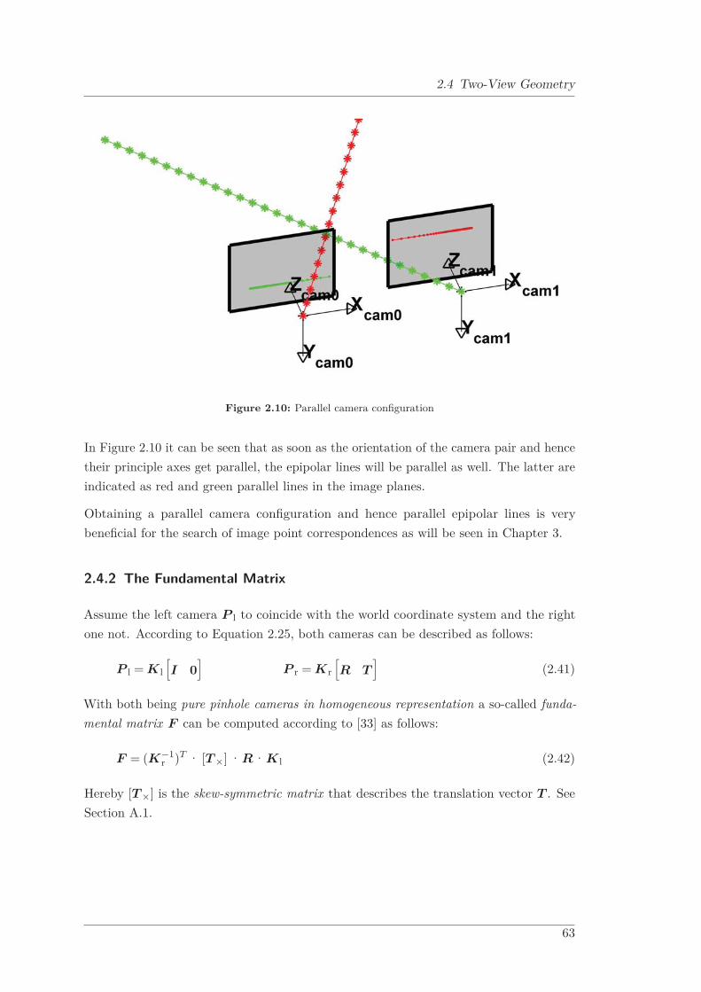
2.4 Two-View Geometry
Figure 2.10: Parallel camera configuration
In Figure 2.10 it can be seen that as soon as the orientation of the camera pair and hencetheir principle axes get parallel, the epipolar lines will be parallel as well. The latter areindicated as red and green parallel lines in the image planes.
Obtaining a parallel camera configuration and hence parallel epipolar lines is verybeneficial for the search of image point correspondences as will be seen in Chapter 3.
2.4.2 The Fundamental Matrix
Assume the left camera P l to coincide with the world coordinate system and the rightone not. According to Equation 2.25, both cameras can be described as follows:
P l = K l[I 0
]P r = Kr
[R T
](2.41)
With both being pure pinhole cameras in homogeneous representation a so-called funda-mental matrix F can be computed according to [33] as follows:
F = (K−1r )T · [T ×] ·R·K l (2.42)
Hereby [T ×] is the skew-symmetric matrix that describes the translation vector T . SeeSection A.1.
63

2 Fundamentals of Computer Vision Geometry
As described in Section 2.4.1, a corresponding image point X img,r with respect to theimage point X img,l can be found on the epipolar line le,r. In other words, epipolargeometry provides for every image point in the left view a corresponding line in the rightone - and vice versa. This mapping is performed by the fundamental matrix F and iscalled epipolar constraint. A correspondence condition can be formulated as follows:
X imgT,rF X img,l = 0 with le,r = F X img,l (2.43)
F is a 3x3 matrix that is not of full rank (rank (F ) = 2) since it maps points to lines.The operation is not invertible. From corresponding views, F can be estimated with theso-called 8-Point Algorithm as extensively described in [37].
2.4.3 Epipolar Curves
If we consider a pair of cameras employing the pinhole camera model with distortionor as can be seen in Figure 2.11 applying a completely different camera model, theepipolar constraint no longer produces straight lines. Furthermore it gives rise to epipolarcurves.
Figure 2.11: Parallel camera configuration
64

2.4 Two-View Geometry
According to [33] the mathematical relationships of Equation 2.42 and Equation 2.43hence have to be generalized to:
dist
(X img,l,P l
(P −1
r [X img,r]\z = 0))
= 0 and
dist
(X img,r,P r
(P −1
l [X img,l]\z = 0))
= 0(2.44)
Depending on the distinct camera model, the epipolar curves can be described mathemat-ically. For example if the pinhole camera model is applied with a simple radial distortiononly described by one parameter, the resulting curves are cubic. See [139].
If the equiangular model is used as done in Figure 2.11, the resulting curves are so-calledgreat circles, which is the intersection curve of the sphere and a plane passing throughthe cameras principle point. We will later come back to this fact.
65

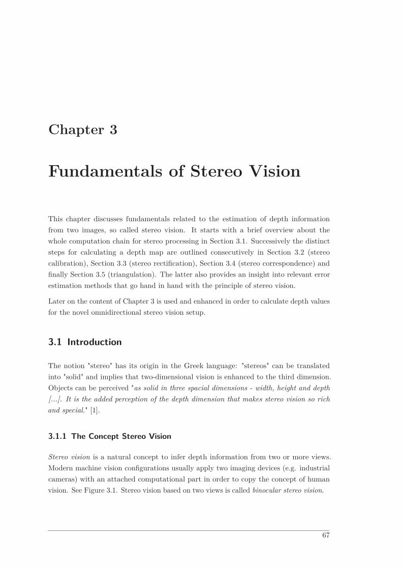
Chapter 3
Fundamentals of Stereo Vision
This chapter discusses fundamentals related to the estimation of depth informationfrom two images, so called stereo vision. It starts with a brief overview about thewhole computation chain for stereo processing in Section 3.1. Successively the distinctsteps for calculating a depth map are outlined consecutively in Section 3.2 (stereocalibration), Section 3.3 (stereo rectification), Section 3.4 (stereo correspondence) andfinally Section 3.5 (triangulation). The latter also provides an insight into relevant errorestimation methods that go hand in hand with the principle of stereo vision.
Later on the content of Chapter 3 is used and enhanced in order to calculate depth valuesfor the novel omnidirectional stereo vision setup.
3.1 Introduction
The notion "stereo" has its origin in the Greek language: "stereos" can be translatedinto "solid" and implies that two-dimensional vision is enhanced to the third dimension.Objects can be perceived "as solid in three spacial dimensions - width, height and depth[...]. It is the added perception of the depth dimension that makes stereo vision so richand special." [1].
3.1.1 The Concept Stereo Vision
Stereo vision is a natural concept to infer depth information from two or more views.Modern machine vision configurations usually apply two imaging devices (e.g. industrialcameras) with an attached computational part in order to copy the concept of humanvision. See Figure 3.1. Stereo vision based on two views is called binocular stereo vision.
67
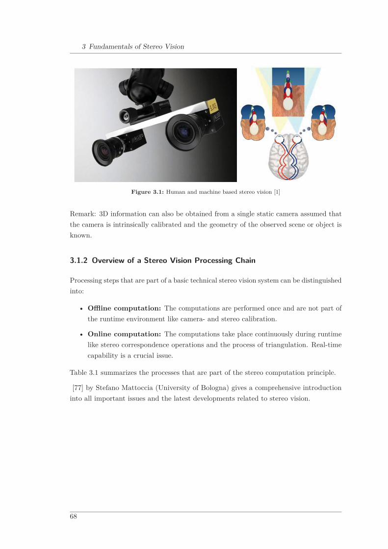
3 Fundamentals of Stereo Vision
Figure 3.1: Human and machine based stereo vision [1]
Remark: 3D information can also be obtained from a single static camera assumed thatthe camera is intrinsically calibrated and the geometry of the observed scene or object isknown.
3.1.2 Overview of a Stereo Vision Processing Chain
Processing steps that are part of a basic technical stereo vision system can be distinguishedinto:
• Offline computation: The computations are performed once and are not part ofthe runtime environment like camera- and stereo calibration.
• Online computation: The computations take place continuously during runtimelike stereo correspondence operations and the process of triangulation. Real-timecapability is a crucial issue.
Table 3.1 summarizes the processes that are part of the stereo computation principle.
[77] by Stefano Mattoccia (University of Bologna) gives a comprehensive introductioninto all important issues and the latest developments related to stereo vision.
68
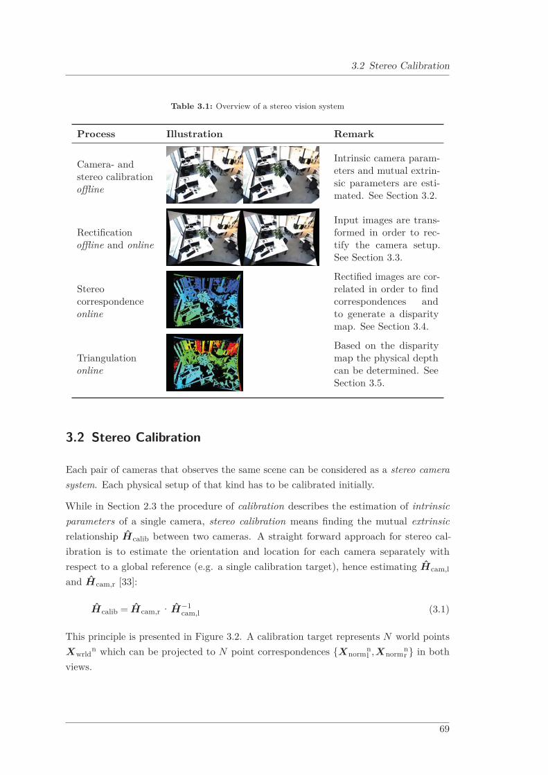
3.2 Stereo Calibration
Table 3.1: Overview of a stereo vision system
Process Illustration Remark
Camera- andstereo calibrationoffline
Intrinsic camera param-eters and mutual extrin-sic parameters are esti-mated. See Section 3.2.
Rectificationoffline and online
Input images are trans-formed in order to rec-tify the camera setup.See Section 3.3.
Stereocorrespondenceonline
Rectified images are cor-related in order to findcorrespondences andto generate a disparitymap. See Section 3.4.
Triangulationonline
Based on the disparitymap the physical depthcan be determined. SeeSection 3.5.
3.2 Stereo Calibration
Each pair of cameras that observes the same scene can be considered as a stereo camerasystem. Each physical setup of that kind has to be calibrated initially.
While in Section 2.3 the procedure of calibration describes the estimation of intrinsicparameters of a single camera, stereo calibration means finding the mutual extrinsicrelationship Hcalib between two cameras. A straight forward approach for stereo cal-ibration is to estimate the orientation and location for each camera separately withrespect to a global reference (e.g. a single calibration target), hence estimating Hcam,l
and Hcam,r [33]:
Hcalib = Hcam,r ·H−1cam,l (3.1)
This principle is presented in Figure 3.2. A calibration target represents N world pointsXwrld
n which can be projected to N point correspondences {Xnormnl ,Xnorm
nr } in both
views.
69

3 Fundamentals of Stereo Vision
Figure 3.2: The principle of stereo calibration
Hanning [33] states that this basic approach is not accurate enough for stereo visionand must be enhanced by using multiple target positions. Commonly the new globalreference then coincides with the left camera coordinate system as already mentioned inEquation 2.41.
According to Hanning [33] calibration approaches for stereo configurations can be catego-rized as follows:
• Extrinsic stereo camera calibration with generalized epipolar constraints
• Extrinsic stereo camera calibration with respect to the projective error
• Extrinsic and intrinsic stereo camera calibration
Table 3.2 summarizes related work with regards to stereo calibration. In the following aprocedure based on minimizing the projective error is considered.
3.2.1 Extrinsic Stereo Calibration With Respect to the Projective Error
If we assume both cameras to be distortion-free (all intrinsic parameters are known), apossible calibration process can be described as follows: A setup as seen in Figure 3.2 isused to generate N point correspondences {Xnorm
mnl ,Xnorm
mnr } (left and right camera)
for each of M arbitrary positioned calibration targets. The key points of the targetrepresent the world points Xwrld.
70

3.2 Stereo Calibration
Table 3.2: Summary of publications that consider stereo calibration
Year Author(s) Remark Publications
1990 Juyang Wenget al.
Two-step calibration method: (1) pa-rameter estimation based on distortion-free camera model. (2) Non-linear opti-mization step.
[127]
1996 Fuxing Liet al.
Computes the fundamental matrix withan active moving stereo camera pairwith common elevation platform.
[65]
1996 Zhengyou Zhang Overview paper of different methods,that compute the fundamental matrix. [138–140]
1999 Richard Hartley
Overview paper of different meth-ods, that calibrate stereo vision sys-tems. Compares strong, weak and non-calibrated geometries.
[35]
2004,2006,2011
Tobias Hanninget al.
Treatment of a generalized approach forthe epipolar connection between two im-ages and derivation of a special calibra-tion method.
[32–34]
2005Niklas PetterssonandLars Petersson
Suggests a method of online calibrationfor moving camera pairs. [98]
2006 Chuan Zhouet al.
A stereo calibration method speciallyfor wide-angled lenses is investigated. [143]
2007 Hyukseong Kwonet al.
A closed-form solution for online cal-ibration for moving (panning, tilting)camera pairs.
[63]
The world points can be projected to both cameras. This can be modelled as follows:
Xnormmnl = RlXwrld
mn +T l and Xnormmnr = RrXwrld
mn +T r (3.2)
where Rl, and Rr are the unknown rotation matrices for the left and the right camera. T l,and T r represent unknown translations for both views. Both equations of Equation 3.2 canbe combined in order to remove the world point Xwrld
mn and establish the relationshipbetween left and right view:
Xnormmnr = RrR
Tl ·Xnorm
mnl −RrR
Tl ·T l +T r (3.3)
Further simplification leads to:
Xnormmnr = R·Xnorm
mnl +T with R = RrR
Tl and T = −RrR
Tl ·T l +T r (3.4)
71

3 Fundamentals of Stereo Vision
The average values of the computed parameters R and T represent the complete extrinsicrelationship Hcalib between both cameras. They can be further refined by a non-linearoptimization step and form the precondition for the process of stereo rectification.
3.3 Stereo Rectification
After calibrating each camera intrinsically (K l, Kr) as well as estimating the mutualextrinsic relationship (Hcalib), the stereo system needs to be rectified. In Figure 3.3the rectification process is illustrated. Two cameras in general position with the mutualextrinsic relationship of Hcalib need to be rotated to fulfil two requirements:
1. x-axes are collinear and z-axes (optical axes) are parallel.
2. Intrinsic parameters are identical.
The positions of the cameras cannot be changed since they are connected rigidly. Theactual computation takes place offline as part of the stereo calibration process.
Figure 3.3: The principle of stereo rectification
Since one cannot rotate the cameras physically, a transformation has to be applied tothe images itself. This is done by appropriate image transformation mappings.
72
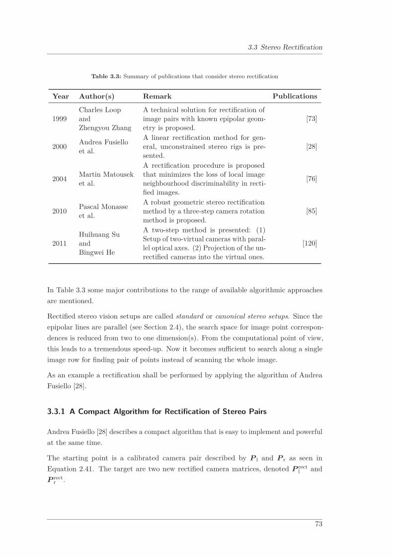
3.3 Stereo Rectification
Table 3.3: Summary of publications that consider stereo rectification
Year Author(s) Remark Publications
1999Charles LoopandZhengyou Zhang
A technical solution for rectification ofimage pairs with known epipolar geom-etry is proposed.
[73]
2000 Andrea Fusielloet al.
A linear rectification method for gen-eral, unconstrained stereo rigs is pre-sented.
[28]
2004 Martin Matouseket al.
A rectification procedure is proposedthat minimizes the loss of local imageneighbourhood discriminability in recti-fied images.
[76]
2010 Pascal Monasseet al.
A robust geometric stereo rectificationmethod by a three-step camera rotationmethod is proposed.
[85]
2011Huihuang SuandBingwei He
A two-step method is presented: (1)Setup of two-virtual cameras with paral-lel optical axes. (2) Projection of the un-rectified cameras into the virtual ones.
[120]
In Table 3.3 some major contributions to the range of available algorithmic approachesare mentioned.
Rectified stereo vision setups are called standard or canonical stereo setups. Since theepipolar lines are parallel (see Section 2.4), the search space for image point correspon-dences is reduced from two to one dimension(s). From the computational point of view,this leads to a tremendous speed-up. Now it becomes sufficient to search along a singleimage row for finding pair of points instead of scanning the whole image.
As an example a rectification shall be performed by applying the algorithm of AndreaFusiello [28].
3.3.1 A Compact Algorithm for Rectification of Stereo Pairs
Andrea Fusiello [28] describes a compact algorithm that is easy to implement and powerfulat the same time.
The starting point is a calibrated camera pair described by P l and P r as seen inEquation 2.41. The target are two new rectified camera matrices, denoted P rect
l andP rect
r .
73
3 Fundamentals of Stereo Vision
Computation of the new Rotation Matrices
In order to obtain new rectified rotation matrices Rrectl and Rrect
r , new camera framevectors xrect, yrect and zrect describing the coordinate system of the rectified camerasare computed. They will compose the new matrices Rrect
l and Rrectr .
The new x-axis xrect (see Figure 3.3) points from the origin of the left camera to theorigin of the right one:
xrect =C l −Cr
‖C l −Cr‖ =−Cr
‖−Cr‖ (3.5)
The new y-axis yrect is orthogonal to xrect and k.
yrect = xrect ×k (3.6)
where k is a unit vector that fixes the position of the new y-axis in the plane orthogonalto xrect. k can be successively computed from both z-axes as follows:
k =12
(zl +zr) (3.7)
The algorithm fails when the optical axis is parallel to the base line (e.g. when there is apure forward motion), but this is not relevant for stereo vision setups.
The new z-axis is orthogonal to both x- and y-axis:
zrect = xrect ×yrect (3.8)
The new rotation matrix Rrect that must be identical for both cameras in order to obtainthe same orientation for both views as can be seen in Figure 3.3 can be composed asfollows:
Rrect =
⎡⎢⎢⎢⎣xrectT
yrectT
zrectT
⎤⎥⎥⎥⎦ (3.9)
Computation of the new Camera Calibration Matrix
In principle the new camera calibration matrix Krect can be chosen freely, but shouldmeet some requirements:
• The same matrix Krect must be assigned to both cameras.
• Krect should be adopted from the camera that provides the largest FOV.
74
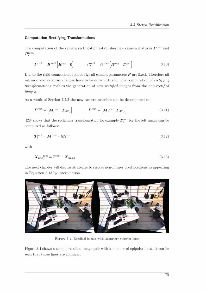
3.3 Stereo Rectification
Computation Rectifying Transformations
The computation of the camera rectification establishes new camera matrices P rectl and
P rectr :
P rectl = Krect
[Rrect 0
]P rect
r = Krect[Rrect T rect
](3.10)
Due to the rigid connection of stereo rigs all camera parameters P are fixed. Therefore allintrinsic and extrinsic changes have to be done virtually. The computation of rectifyingtransformations enables the generation of new rectified images from the non-rectifiedimages.
As a result of Section 2.2.2 the new camera matrices can be decomposed as:
P rectl =
[M rect
l P 4C,l
]P rect
r =[M rect
r P 4C,r
](3.11)
[28] shows that the rectifying transformation for example T rectl for the left image can be
computed as follows:
T rectl = M rect
l ·M l−1 (3.12)
with
X imgrect,l = T rect
l ·X img,l (3.13)
The next chapter will discuss strategies to resolve non-integer pixel positions as appearingin Equation 3.13 by interpolation.
Figure 3.4: Rectified images with exemplary epipolar lines
Figure 3.4 shows a sample rectified image pair with a number of epipolar lines. It can beseen that those lines are collinear.
75

3 Fundamentals of Stereo Vision
3.4 Stereo Correspondence
In order to exploit two images for depth computation, the next step has to find pairs ofpoints that belong to identical scene details. This aspect is known as stereo correspondenceproblem and describes the challenge to find for each pixel X img,l from the left image acorresponding pixel X img,r in the right one.
3.4.1 Disparity Computation
After aligning the epipolar lines collinearly, the actual correspondence search for apoint X img,l in the left image can take place on the same row in the right image - cf.Section 2.4.
Figure 3.5: The principle of disparity computation
Figure 3.5 illustrates the correspondence search for a point X img,l in the left image(intersection of red and blue line). The search takes place in the right image on the redline and leads to the corresponding point X img,r (intersection of red and magenta line)and hence the disparity d:
d = ximg,l −ximg,r (3.14)
• The disparity d is the horizontal displacement of conjugate image points. [d] = px
A two-dimensional matrix D of disparity values d assigned to each pixel X img,l in theleft image is called a disparity map. A color coded example is outlined in Figure 3.6.
Black areas represent regions in the left image for which no corresponding points in theright image could be found.
76

3.4 Stereo Correspondence
Figure 3.6: Colour coded disparity map
3.4.2 The Correspondence Problem
Finding corresponding pixels is the crucial point for stereo vision and has recently attractedconsiderable interest amongst many researchers. On the Middlebury website [108] modernalgorithms are evaluated and ranked competitively. For benchmarking they provide aframework and an appropriate dataset as can be seen exemplary in Table 3.4.
Challenges for Stereo Correspondence Approaches
Algorithms that correlate two images have to face remaining image distortions and pixelnoise, reflecting, transparent and specular surfaces, perspective distortions due to differentcamera positions, homogeneous and ambiguous regions as well as repetitive patterns.Furthermore occlusions and discontinuities create problems for the stereo methods.
In contrast microcomputer architectures for possible target platforms of embeddedsolutions limit the amount of available computational power.
A Taxonomy of Stereo Algorithms
Scharstein et al. [107] sketch a taxonomy and evaluation of dense two-frame stereocorrespondence algorithms. Generally, these approaches can be distinguished into:
77

3 Fundamentals of Stereo Vision
Table 3.4: Evaluation dataset of Middlebury website
Name Left Image Right Image Ground Truthof Left Image Reference
Cones [106]
Teddy [40,105]
Aloe [40,105]
• Local algorithms: They perform a so-called Winner Takes it All (WTA) selectionstrategy for image correspondences. Pixel value ambiguities are reduced by aggre-gating matching costs over a support window (also known as kernel or correlationwindow). This increases the Signal to Noise Ratio (SNR). [77].
• (Semi-) global algorithms: These algorithms search for disparity assignmentsthat minimize an energy function over the whole stereo pair using a pixel-basedmatching cost (sometimes the matching cost is aggregated over a support). [77].
According to Scharstein et al. [107], common stereo algorithms consist of the followingsteps: (1.) matching cost computation, (2.) cost aggregation, (3.) disparity computationand optimization, (4.) disparity refinement.
One of the most commonly used algorithms are the local (kernel window based) methods.Using the standard Sum of Squared Differences (SSD) algorithm, the following steps areperformed:
1. Matching cost computation: The matching cost is the squared difference ofintensity values at a given disparity.
2. Cost aggregation: Aggregation is done by summing matching cost over squarewindows with constant disparity.
78
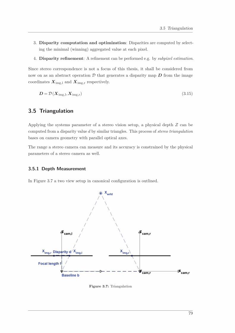
3.5 Triangulation
3. Disparity computation and optimization: Disparities are computed by select-ing the minimal (winning) aggregated value at each pixel.
4. Disparity refinement: A refinement can be performed e.g. by subpixel estimation.
Since stereo correspondence is not a focus of this thesis, it shall be considered fromnow on as an abstract operation D that generates a disparity map D from the imagecoordinates X img,l and X img,r respectively.
D = D (X img,l,X img,r) (3.15)
3.5 Triangulation
Applying the systems parameter of a stereo vision setup, a physical depth Z can becomputed from a disparity value d by similar triangles. This process of stereo triangulationbases on camera geometry with parallel optical axes.
The range a stereo camera can measure and its accuracy is constrained by the physicalparameters of a stereo camera as well.
3.5.1 Depth Measurement
In Figure 3.7 a two view setup in canonical configuration is outlined.
Figure 3.7: Triangulation
79

3 Fundamentals of Stereo Vision
According to Chang et al. [17] a depth value Z can be estimated from Equation 3.16.
Z = b·f
ad(3.16)
where
• a is the physical pixel width and hence the image sampling interval. It is identicalwith px (see Section 2.2.1.2). [a] = mm.
By using the intrinsic parameters of the camera calibration matrix K, the equation canbe re-expressed as follows:
Z = b·αx
ximg,l −ximg,r= b·
αx
d(3.17)
Each depth value Z represents the z-component of a 3D point given in camera coordi-nates.
3.5.2 Range Field of Measurement
According to Mattoccia [77] the range of operation [Zmax,Zmin], so-called horopter, isconstrained by the disparity range [dmin,dmax].
• dmin: The minimal measurable disparity is 0.5. This concludes that the maximumdistance that can be measured directly depends on the spacial resolution of theworking camera. [dmin] = px.
• dmax: The maximal measurable disparity depends on the parametrization. Thishas to be balanced between a required closest area that should be measurable andthe desired observable horizontal field of view FOVh. The latter is directly reducedby the maximum disparity. This effect can be observed in Figure 3.6 as a black(blind) left margin. [dmax] = px.
3.5.3 Measurement Accuracy
Measurement accuracy arises from the limited image resolution given by a. The accuracyof depth measurements of a stereo vision system is denoted as depth resolvability Z∗ andcan be calculated as follows:
Z∗ =bf
a∗ , a∗ =a
2(3.18)
where
• Z∗ is the depth resolvability. [Z∗] = mm.
80

3.5 Triangulation
Figure 3.8: Horopter
• a∗ is the image resolution with a∗ = a2 . [a∗] = mm.
According to Chang [17] the depth resolvability "[...] represents the maximum depthresolvable by the given stereo imaging system.".
If the disparities (to measure) are less than a∗, and hence Z > Z∗, the origin points haveto be considered as points with Z at infinity:
{a∗ → 0} ⇒ {Z∗ → ∞} (3.19)
3.5.4 Measurement Errors
Following Chang [17] the reasons of erroneous measurements in stereo vision are due to avast amount of factors:
• Angular errors: They result from the fact that the image plane is not exactlyperpendicular to the camera axis.
• Rotation error: There is a certain rotational offset between camera and imagecoordinate system.
• Position error: The imager is not sufficiently flat.
81
3 Fundamentals of Stereo Vision
Additional errors are focal length error, quantization error and mismatching errors, toname a few more. For further procedure it is assumed that a depth estimation error onlyarises due to spacial quantization effects in the image plane. Following the explanationsof [27] and [4] an analysis of errors for stereo vision can be regarded as an geometrical issue,an statistical issue as well as from the viewpoint of geometrical qualities. Section 3.5.4.1and Section 3.5.2 review the error computation from the aspects of geometry and statisticsin more detail.
3.5.4.1 Quantization Error
A depth measurement error can be specified as absolute depth error δZ as well aspercentage depth error δZ/Z:
δZ = δZb + δZf + δZd =f
dδb+
b
dδf − bf
d2 δd (3.20)
and
δZ
Z=
δb
b+
δf
f− δad
ad(3.21)
where
• δZb denotes the partial derivative of Z with respect to b. [δZb] = mm.
• δZf denotes the partial derivative of Z with respect to f . [δZf ] = mm.
• δZd denotes the partial derivative of Z with respect to d. [δZd] = mm.
As a consequence of Equation 3.20 and Equation 3.21, the major contributions to δZ
are drawn by the baseline inaccuracy δb, focal length error δf and disparity error δd.According to Chang [17] the contributions δb and δf to the overall error value canbe neglected for accurate devices. Hence the afore-mentioned error quantities can besimplified to:
δZ ≈ −Z2δd
bf(3.22)
and
‖δZ‖Z
≈ Z‖δd‖bf
(3.23)
82

3.5 Triangulation
Figure 3.9: Example quantization error
Figure 3.9 shows an exemplary quantization error plot for an artificial stereo vision setupwith the parameters f = 3.5mm, b = 10cm and px = 5μm.
From Equation 3.22 and Figure 3.9 it can be concluded that the depth error is quadraticallydependent on Z and proportional to δd. Furthermore from Equation 3.23 and Figure 3.9it can be concluded that the percentage depth error depends linearly on Z.
A deviation of δZ can be reviewed in Section A.2.
3.5.4.2 Statistical Distribution of Quantization Errors
A further way to examine error occurrences is to describe a probability distribution ofthe range error and the expected value of range error magnitude.
Following Chang [17] a probability density function p for the likelihood of δZ in a stereovision geometry can be stated as follows:
p(δZ) =
⎧⎪⎨⎪⎩Z∗
2ZmaxZmin− (Z∗)2(Zmin2+ZminZmax+Zmax2)
12(ZminZmax)3 · |δZ| if 0 ≤ |δZ| ≤ 2Zmin2
Z∗
1Zmax−Zmin
[23
√Z∗
2|δZ| + (Z∗)2
12Zmax3 · |δZ|− Z∗2Zmax
]if 2Zmin2
Z∗ ≤ |δZ| ≤ 2Zmax2
Z∗
(3.24)
83

3 Fundamentals of Stereo Vision
A deviation of p(δZ) can be reviewed in Section A.3. There it can be studied that thedepth Z to measure can be considered as a random variable between a minimal depthZmin and a maximum depth Zmax.
The information of the probabilistic distribution p(δZ) can be further conditioned to geta statement about the expected magnitude of the absolute depth error E(|δZ|) which isdefined as:
E(|δZ|) =∫ +∞
−∞f(Z)E(|δZ||Z)dZ (3.25)
Rodriguez et al. [100] derive the expected absolute depth error in magnitude for the caseof uniformly distributed depth over the interval [Zmin, Zmax] to be:
E(|δZ|) =2
9Z∗(Zmax
2 +ZminZmax +Zmin2)
(3.26)
The complete derivation from Equation 3.25 to Equation 3.26 can be reviewed in [100].
For an exemplary stereo vision setup with f = 1.0mm, b = 10cm and px = 5μm thegraphic Figure 3.10 demonstrates the normalized probability density function pn (δZ)and the expected absolute depth error E(|δZ|) at a target depth Z = 2.5m, with:
pn (δZ) =p(δZ)
max(p(δZ))(3.27)
Figure 3.11 presents a selection of the left cameras pixels re-projected to their appropriatecamera rays. The probability distribution of the measured depth Z has been illustratedas color coded plot. It is visible that the measurement of euclidean distances of camerapoints Xcam for a constant target depth Z is most accurate at the (perspective) camerascenter.
84

3.5 Triangulation
Figure 3.10: Sample probability distribution of δZ at Z = 2.5m (2D)
Figure 3.11: Sample probability distribution of δZ at Z = 2.5m (3D)
85

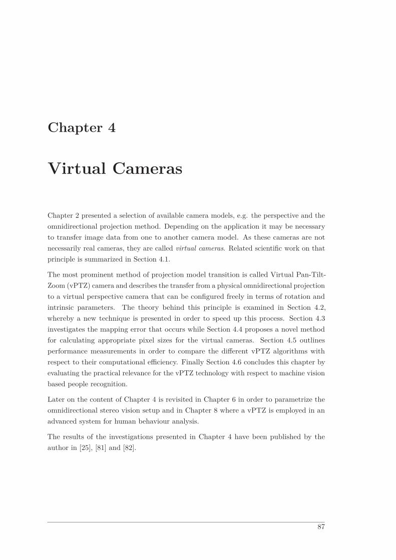
Chapter 4
Virtual Cameras
Chapter 2 presented a selection of available camera models, e.g. the perspective and theomnidirectional projection method. Depending on the application it may be necessaryto transfer image data from one to another camera model. As these cameras are notnecessarily real cameras, they are called virtual cameras. Related scientific work on thatprinciple is summarized in Section 4.1.
The most prominent method of projection model transition is called Virtual Pan-Tilt-Zoom (vPTZ) camera and describes the transfer from a physical omnidirectional projectionto a virtual perspective camera that can be configured freely in terms of rotation andintrinsic parameters. The theory behind this principle is examined in Section 4.2,whereby a new technique is presented in order to speed up this process. Section 4.3investigates the mapping error that occurs while Section 4.4 proposes a novel methodfor calculating appropriate pixel sizes for the virtual cameras. Section 4.5 outlinesperformance measurements in order to compare the different vPTZ algorithms withrespect to their computational efficiency. Finally Section 4.6 concludes this chapter byevaluating the practical relevance for the vPTZ technology with respect to machine visionbased people recognition.
Later on the content of Chapter 4 is revisited in Chapter 6 in order to parametrize theomnidirectional stereo vision setup and in Chapter 8 where a vPTZ is employed in anadvanced system for human behaviour analysis.
The results of the investigations presented in Chapter 4 have been published by theauthor in [25], [81] and [82].
87

4 Virtual Cameras
4.1 Introduction and Related Works
The generation of perspective views from an omnidirectional image has already beenpicked up in previous scientific work.
Peri et al. [97] developed a software system which is able to generate multiple perspec-tive and panoramic views from an omnidirectional image. As an input source of theomnidirectional image serves a catadioptric camera system consisting of a conventionalcamera and a parabolic mirror. Virtual cameras, placed and parametrized by the user,generate the different views. The pixel intensity on the imaging surface of such a virtualcamera is determined by reprojection on the parabolic mirror. To process in real-time, ageometric map is generated for each view only once. As long as the viewing parametersof the virtual camera are not changed, the reprojection can be sped up by a Look-UpTable (LUT). However, the omnidirectional projection of the catadioptric camera is onlyestimated with a relatively simple parabolic equation.
Onoe et al. [93] improved the algorithm with the aim of a faster perspective imagegeneration. They divided the destination image into equal parts using a rectangular grid.Each grid point is reprojected in the omnidirectional image, whereas four grid pointsalways form a quadrilateral. Each quadrilateral in the omnidirectional image is warped tothe corresponding position in the perspective image applying a bi-linear interpolation. Inthis way the quality of the perspective image is reduced in favour of a faster calculation.Similar to Peri et al., they used a catadioptric camera and model the image formation byapplying an equation for the hyperboloidal surface of the mirror.
Zhang et al. [136] used a camera with a fisheye lens. They modelled the lens with asphere on whose surface the omnidirectional image is projected. The computationalexpensive rectification algorithm was implemented on a Field Programmable Gate Array(FPGA) for the purpose of real-time processing.
The approaches presented above share a common disadvantage. They lack a precise andgeneric camera model to describe various off-the-shelf cameras - cf. Section 2.2.4.
An mentionable application for the generation of a panoramic image from an omnidirec-tional image was presented by Ardouin et al. [5]. There, a catadioptric camera system ismounted on a helmet. A captured omnidirectional image is transformed into a panoramicimage. The result is displayed on an HMD. So a person wearing that helmet experiencesa 360◦ surround view.
Table 4.1 provides an overview of relevant scientific contributions to this topic.
The following sections detail the afore-mentioned technology.
88

4.1 Introduction and Related Works
Table 4.1: Summary of scientific contributions to methods of camera model conversion
Year Author(s) Remark Publications
1997 Peri et al.Generation of perspective andpanoramic views from a catadioptriccamera system
[97]
1998 Onoe et al.Generation of perspective views from acatadioptric camera system by applyingan LUT
[93]
2002 Peter Sturm
Analysis of relations between multipleviews of different camera types (para-catadioptric, perspective or affine cam-eras)
[119]
2003Tarak GandhiandMohan M. Trivedi
Parametric ego-motion compensationwith an omnidirectional camera [30]
2003 Chiharu Ishiiet al.
Consideration of omni-directional visionusing an equidistant projection fish eyelens; a partial domain of an originalimage in fish eye image is selected, andthis is converted to a perspective image
[45]
2004,2007,2008
Sheng-Wen JengandWen-Hsiang Tsai
Construction of perspective andpanoramic images from omnidirectionalimages taken from hypercatadioptriccameras
[47–49]
2007 Simon Thibault
Surveillance system featuring apanoramic panomorph lens for eventdetection, recognition and identificationover a 360-degree area with 100 percentcoverage
[124]
2008 Zhang et al.Rectification of a fish-eye lens basedimage by modelling the projection witha sphere on a FPGA architecture
[136]
2012 Ardouin et al.Generation of a panoramic image froman omnidirectional image for a HeadMounted Display (HMD)
[5]
2013 Michel Findeisenet al.
A fast approach for omni- to perspectiveimage conversion and error analysis [25]
89

4 Virtual Cameras
4.2 Omni to Perspective Vision
In order to transform an omnidirectional image into one or multiple perspective images,several approaches are available as presented in Section 4.1.
The method introduced now treats the perspective images as the result of n virtu-ally distributed perspective cameras Camper
0 , . . . ,Camperi , . . . ,Camper
n that are completelydescribed by their extrinsic parameters Cper
i , Rperi and intrinsic parameters Kper
i asdiscussed in Section 2.2.
The omnidirectional camera is described by its extrinsic parameters Comni, Romni andits intrinsic parameters Komni, which are fixed and provided by the physical mount andconstruction of the fisheye camera. These parameters are determined during the cameracalibration procedure. Furthermore the projection behaviour of the omnidirectionalcamera is described by its projection model as seen in Section 2.2.
For the virtual perspective views the extrinsic calibration of the omnidirectional cameraforms the world reference. Hence the parameters Cper
i and Rperi refer to Comni and
Romni. Since the location of every Camperi is identical with Comni, Cper
i = 0 (3 DOF arefixed), while its rotation Rper
i can be chosen freely with reference to Romni (3 DOF arevariable). Furthermore, Kper
i can be chosen freely.
Figure 4.1 shows a sample setup comprising an omnidirectional camera (with the imagefrom Figure 2.8 mapped onto a sphere - cf. Section 2.2.3) and a single perspective camera(with a plane sensor surface - cf. Section 2.2.2).
After having set up the omnidirectional camera as well as at least one virtual perspectivecamera, perspective images can be generated using one of two possible mapping strategies:Forward Mapping or Backward Mapping. Both strategies are explained in Section 4.2.1and Section 4.2.2. For the latter an enhanced process is presented in Section 4.2.3 denotedas Fast Backward Mapping.
4.2.1 Forward Mapping
The principle of forward mapping shapes the algorithm in a way that the computationsequence starts at the omnidirectional image source and ends at the perspective imagetarget. The mapping algorithm can be summarized as outlined in Figure 4.2.
The remainder of this subsection treats each step in more detail.
Back-Projection (Source): The color information as seen in Figure 4.1 relates to agrid of two-dimensional pixel coordinates Xomni
img . The full grid Xomniimg is back-projected
to their appropriate 3D rays, described as Cartesian expression Xomnicam with respect to
the omnidirectional camera coordinate system.
90
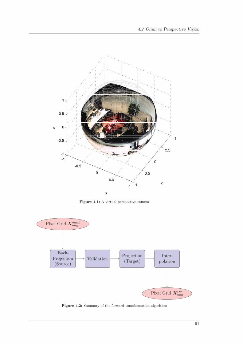
4.2 Omni to Perspective Vision
Figure 4.1: A virtual perspective camera
Pixel Grid Xomniimg
Back-Projection(Source)
ValidationProjection(Target)
Inter-polation
Pixel Grid Xperimg
Figure 4.2: Summary of the forward transformation algorithm
91

4 Virtual Cameras
Therefore Xomniimg is transferred to its normalized sensor coordinates Xomni
norm by employingEquation 2.15 inversely:
Xomninorm = K−1 ·Xomni
img (4.1)
In the successive stage, Xomninorm is represented by appropriate polar coordinates - cf.
Equation 2.6 and Equation 2.7:
Xomninorm =
⎛⎜⎜⎜⎝xomni
norm
yomninorm
1
⎞⎟⎟⎟⎠ =
⎛⎜⎜⎜⎝ρomni
norm
ϕomninorm
1
⎞⎟⎟⎟⎠ (4.2)
Using Equation 2.8 and Equation 2.29, hence employing generic back-projection, theappropriate camera points can be set up by applying the following relationship:
Xomnicam =
⎛⎜⎜⎜⎜⎜⎜⎝xomni
cam
yomnicam
zomnicam
womnicam
⎞⎟⎟⎟⎟⎟⎟⎠ =
⎛⎜⎜⎜⎝θomni
cam
ϕomnicam
ρomnicam
⎞⎟⎟⎟⎠ =
⎛⎜⎜⎜⎝K−1(ρomni
norm)ϕomni
norm
1
⎞⎟⎟⎟⎠ (4.3)
where Xomnicam is expressed as spherical coordinates (θomni
cam ,ϕomnicam ,ρomni
cam )T with ρomnicam being
the distance of the 3D point from the origin Comni. To overcome the uncertainty ofthe distance between the point in camera coordinates and the camera center, chooseρomni
cam =∥∥∥Xomni
cam
∥∥∥ != 1 to normalize the points to a unity sphere.
Validation: The following stage treats the imaging process of Xomnicam into the virtual
perspective camera Camper. An omnidirectional camera covers a considerably larger FOVthan a perspective one. Back-projected image points Xomni
cam might partially have negativezper-components which, if projected, lead to non-valid image points. Those points haveto be neglected. Referring to Figure 2.6, valid 3D points have to reside rightwards of p3R
(principle plane). Hence those points comply with the following equation:
p3R ·Xomnicam ≥ 0 (4.4)
Projection (Target): Now Xomnicam can be projected into the perspective camera model
by applying Equation 2.24:
Xperimg = P ·Xomni
cam (4.5)
This can be done since Xomnicam = Xper
wrld. Performing Equation 4.5 leads to real-numbertarget image pixel positions X
perimg. To distinguish between integer and real-number
coordinates, the latter is indicated by X.
92

4.2 Omni to Perspective Vision
Interpolation: In order to obtain pixel intensities Iper of the integer coordinates Xperimg =
(xperimg,yper
img,1)T from the real-number pixel positions Xperimg and its appropriate pixel
intensities Iomni a standard image interpolation procedure (e.g. bilinear or bi-cubic) isemployed.
The forward procedure has significant disadvantages. Regardless of the specification of thevirtual target camera, the complete set of source image coordinates is transformed despitenot all coordinates being within the visible range of the target image. Furthermore, ifapplying an accurate generic camera model as presented in Section 2.2.4, the mathematicalrelationship has to be solved inversely by finding the roots of Kannala’s polynomial. Thisleads to a tremendous lack of performance. Another important aspect is the fact that theuse of low order interpolation filters, like bilinear or bi-cubic filter masks, can producegaps in the target images if the source pixel positions map onto the target pixel positionsin a sparse distribution.
An exemplary perspective result can be reviewed in Figure 4.3.
Figure 4.3: Result forward projection
4.2.2 Backward Mapping
An alternative approach can overcome the disadvantages mentioned in the previoussection while offering further possibilities to improve performance. Backward mappinginverses the problem - from target to source. The mapping algorithm can be summarizedas outlined in Figure 4.4.
The remainder of this subsection treats each step in detail.
93

4 Virtual Cameras
Pixel Grid Xperimg
Back-Projection(Target)
Projection(Source)
Inter-polation
Pixel Grid Xomniimg
Figure 4.4: Summary of the backward transformation algorithm
Back-Projection (Target): Equivalently to Section 4.2.1, the target image mesh ofpixel positions Xper
img is set up and back-projected to its appropriate world points Xperwrld
using Equation 2.24 inversely:
Xperwrld (λ) = λ·P + ·Xper
img (4.6)
where P + forms the pseudo-inverse of P and λ is an arbitrary scale factor that expressesthe one dimensional space of points on the ray. To overcome the uncertainty of distancefrom the camera center, choose ‖Xper
wrld‖ != 1. See Figure 4.5.
Projection (Source): Project all the normalized world points Xperwrld into the omnidi-
rectional camera model using Equations 2.6, 2.15 and 2.29 to obtain real-number sourceimage pixel positions X
omniimg . See Figure 4.6.
Interpolation: In order to obtain pixel intensities Iper of the integer coordinates Xperimg =
(xperimg,yper
img,1)T from the real-number pixel positions Xomniimg and its appropriate pixel
intensities Iomni a standard image interpolation procedure (e.g. bilinear or bi-cubic) isemployed.
An exemplary perspective result can be reviewed in Figure 4.7.
Lookup-Table Operation: The nonlinear transformation between Xperimg and X
omniimg
can be performed using an LUT for faster video processing. Two LUTs mapx and mapy
describe the transformation for x-coordinates and y-coordinates from Xperimg to X
omniimg
separately. An exemplary LUT mapx for the mapping of x-coordinates in a target imageof 640×480 is shown in Figure 4.8.
94

4.2 Omni to Perspective Vision
Figure 4.5: Reprojection of 2D target image coordinates to 3D camera coordinates onto unit sphere
Figure 4.6: Projection of 3D camera coordinates to 2D source image coordinates
95

4 Virtual Cameras
Figure 4.7: Result backward projection
4.2.3 Fast Backward Mapping
In order to accelerate the process of LUT computation, a change of the scale space canbe employed by using a Gaussian pyramid [46] and sub-sampling the space grid thatforms the LUT. The mapping algorithm can be summarized as outlined in Figure 4.9.
Since the LUT (as seen in Figure 4.8) predominantly comprises low order frequencycomponents, a compression should not lead to significant quality loss as will be seenin Section 4.3. To obey the rules of the sampling theorem, it is not sufficient just to
Figure 4.8: Exemplary lookup-table for the backward mapping of target pixel x-coordinates
96
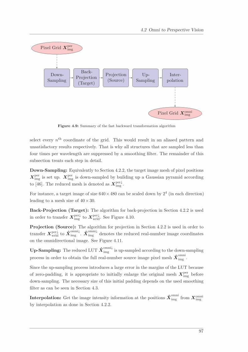
4.2 Omni to Perspective Vision
Pixel Grid Xperimg
Down-Sampling
Back-Projection(Target)
Projection(Source)
Up-Sampling
Inter-polation
Pixel Grid Xomniimg
Figure 4.9: Summary of the fast backward transformation algorithm
select every nth coordinate of the grid. This would result in an aliased pattern andunsatisfactory results respectively. That is why all structures that are sampled less thanfour times per wavelength are suppressed by a smoothing filter. The remainder of thissubsection treats each step in detail.
Down-Sampling: Equivalently to Section 4.2.2, the target image mesh of pixel positionsXper
img is set up. Xperimg is down-sampled by building up a Gaussian pyramid according
to [46]. The reduced mesh is denoted as Xper↓img .
For instance, a target image of size 640×480 can be scaled down by 24 (in each direction)leading to a mesh size of 40×30.
Back-Projection (Target): The algorithm for back-projection in Section 4.2.2 is usedin order to transfer Xper↓
img to Xper↓wrld. See Figure 4.10.
Projection (Source): The algorithm for projection in Section 4.2.2 is used in order totransfer Xper↓
wrld to Xomni↓img . X
omni↓img denotes the reduced real-number image coordinates
on the omnidirectional image. See Figure 4.11.
Up-Sampling: The reduced LUT Xomni↓img is up-sampled according to the down-sampling
process in order to obtain the full real-number source image pixel mesh Xomniimg .
Since the up-sampling process introduces a large error in the margins of the LUT becauseof zero-padding, it is appropriate to initially enlarge the original mesh Xper
img beforedown-sampling. The necessary size of this initial padding depends on the used smoothingfilter as can be seen in Section 4.3.
Interpolation: Get the image intensity information at the positions Xomniimg from Xomni
img
by interpolation as done in Section 4.2.2.
97
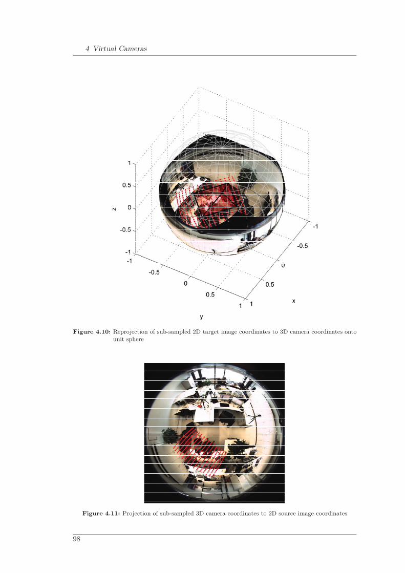
4 Virtual Cameras
Figure 4.10: Reprojection of sub-sampled 2D target image coordinates to 3D camera coordinates ontounit sphere
Figure 4.11: Projection of sub-sampled 3D camera coordinates to 2D source image coordinates
98

4.3 Error Analysis
Lookup-Table Operation: According to Figure 4.8 an exemplary reduced LUT mapxr
connecting the x-coordinates of Xper↓img and X
omni↓img can be seen in Figure 4.12.
0
10
20
30
40
50
60
0
10
20
30
40
50600
800
1000
1200
1400
1600
xy
map
xr
700
800
900
1000
1100
1200
1300
1400
Figure 4.12: Exemplary reduced lookup-table for the fast backward mapping of target pixel x-coordinates
Having up-sampled the data again, an exemplary interpolated LUT connecting thex-coordinates of Xper
img and Xomniimg can be called mapxi.
4.3 Error Analysis
Since the fast backward mapping approach leads to a loss of information, a trade-off inaccuracy has to be accepted to the benefit of a performance improvement. This sectionconsiders the de facto arising error.
Let n be the power of reduction and p× q the target image size. In order to avoid largeerrors at the target image borders as mentioned in Section 4.2, one has to initially padthe original LUTs appropriately. So a convolution of mapx and mapy with the 5 × 5Gaussian kernel
1256
[1 4 6 4 1
]T [1 4 6 4 1
](4.7)
requires a necessary padding of 2n additional pixels on each side. This convolution isdone to smooth the LUTs. In this way we can avoid alias during up-sampling. An erroris introduced during the down- and up-sampling of the LUTs, caused by the dump offrequency components. So it is increasing with the power of reduction n.
99

4 Virtual Cameras
This error can be expressed as a residuum ex and ey in terms of pixel displacementsusing the following equations:
ex = mapx −mapxi (4.8)
ey = mapx −mapyi (4.9)
An example ex for reducing the LUT by the power of 4 can be seen in Figure 4.13.
Figure 4.13: Residuum error for the fast mapping of pixel x-coordinates
The total error exy can be calculated by Equation 4.10.
exy =1pq
∑i,j
(ex
2i,j +ey
2i,j
). (4.10)
Figure 4.14 shows the error exy depending on the elevation of the pinhole camera fordifferent powers of reduction.
Because of symmetrical reasons the error does not depend on the azimuth of the pinholecamera.
As it can be seen, up to a reduction power of n = 4 no significant error can be measured dueto the dominating low order frequency components of the non-linear pixel transformation.For further reduction (n > 4) a noticeable pixel displacement trade-off has to be accepted.Further investigations can be performed in order to determine the distinct mathematicalrelationship between a given acceptable pixel displacement error and the achievablemaximum reduction size.
100

4.4 Accuracy Analysis
1.6 1.8 2 2.2 2.4 2.6 2.8 3 3.210−5
10−4
10−3
10−2
10−1
100
101
102
elevation θ
e xy
n = 1n = 2n = 3n = 4n = 5n = 6n = 7
4
5
6
7
32
1
Figure 4.14: The total pixel error depending on elevation from equator to south pole for each power ofreduction
4.4 Accuracy Analysis
We have seen so far that a conversion from one to another projection model is feasible inan efficient way. The question that shall be answered now is how one can parametrizethe resolution of the virtual target camera based on the physical source camera. In otherwords: how accurate can the target camera be?
The basis for this accuracy discussion for virtual cameras is provided by the intrinsicparameters of the source as well as the target camera. The parameters αx and αy (ofboth cameras) define the physical pixel density (scaled by f) on the (physical and virtual)imaging die in x-direction, and y-direction respectively - cf. Section 2.2.1.2. These valuesdefine the physical pixel width px and py, while each pixel covers a certain solid angle -depending on the underlying camera model. Every physical step px and py representsa pixel step Δximg = 1 and Δyimg = 1 in the image. These parameters represent thephysical sampling interval of the image(er).
101

4 Virtual Cameras
4.4.1 Intrinsics of the Source Camera
Our test system consists of a Fujinon FE185C086HA-1 fisheye lens with a focal lengthof f = 2.7mm and a field of view of 185◦ mounted to a Basler acA2040-25gc industrialcamera containing a 1-inch CMOSIS CMV4000 sensor with a (cropped) resolution of1680×1680 pixels. This camera has been calibrated by using the generic camera model ofKannala [56] which has been summarized in Section 2.2.4. Hereby the radial symmetricmodel applies four polynomial coefficients as outlined in Equation 2.29.
The estimated intrinsic parameters can be found in Table 4.2, while successively computedvalues are presented in Table 4.3.
Table 4.2: Results of the intrinsic generic camera models estimation
Camera k1 k2 αx αy cx cy k3 k4 k5
Camomni 2.40 -0.01 200.25 200.58 838.85 851.67 0.08 -0.05 0.01
Table 4.3: Physical pixel dimensions
Camera px py
Camomni 1.35×10⁻⁵ [m] 1.35×10⁻⁵ [m]
For further distinction of source and target parameters, the pixel densities and pixelwidth values of the source camera are now declared as αomni
x and αomniy as well as pomni
x
and pomniy .
4.4.2 Intrinsics of the Target Camera
In theory, the intrinsic parameters of the virtual (perspective) camera Camper can bechosen freely. A suitable starting point is to define an observable FOV in horizontal andvertical direction: FOVh[rad] and FOVv[rad]. For a distortion-free perspective view thisis determined as follows:
FOVh = 2· arctan(width
2·αx
)= 2· arctan
(width·px
2·f
)FOVv = 2· arctan
(height2·αy
)= 2· arctan
(height·py
2·f
) (4.11)
From Equation 4.11 it becomes obvious that the FOV depends on a bunch of certainintrinsic values:
• If the resolution of the image {width, height} doubles, the size of each virtual pixel{px, py} has to be divided by two for the same FOV.
102
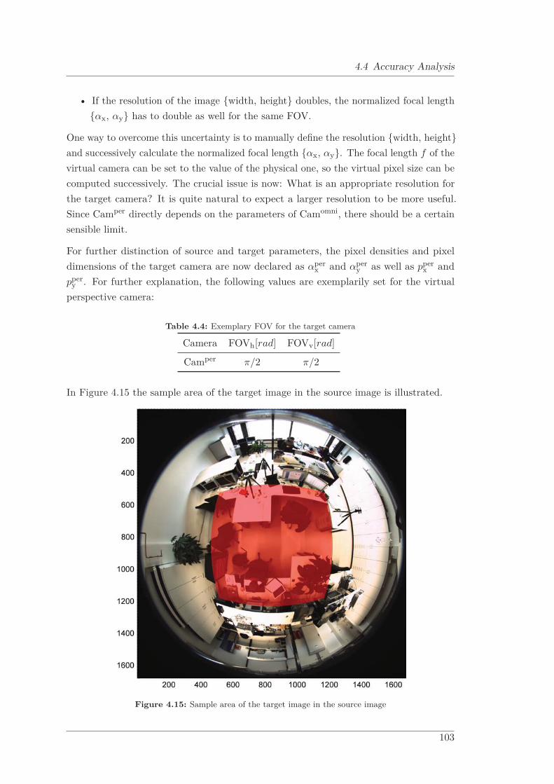
4.4 Accuracy Analysis
• If the resolution of the image {width, height} doubles, the normalized focal length{αx, αy} has to double as well for the same FOV.
One way to overcome this uncertainty is to manually define the resolution {width, height}and successively calculate the normalized focal length {αx, αy}. The focal length f of thevirtual camera can be set to the value of the physical one, so the virtual pixel size can becomputed successively. The crucial issue is now: What is an appropriate resolution forthe target camera? It is quite natural to expect a larger resolution to be more useful.Since Camper directly depends on the parameters of Camomni, there should be a certainsensible limit.
For further distinction of source and target parameters, the pixel densities and pixeldimensions of the target camera are now declared as αper
x and αpery as well as pper
x andpper
y . For further explanation, the following values are exemplarily set for the virtualperspective camera:
Table 4.4: Exemplary FOV for the target camera
Camera FOVh[rad] FOVv[rad]
Camper π/2 π/2
In Figure 4.15 the sample area of the target image in the source image is illustrated.
Figure 4.15: Sample area of the target image in the source image
103
4 Virtual Cameras
4.4.3 Marginal Virtual Pixel Size
From Section 4.4.1 and Section 4.4.2 it becomes obvious that there must be a relationshipbetween the virtual and physical pixel size:
pperx ←
(pomni
x ,pomniy
)pper
y ←(pomni
x ,pomniy
) (4.12)
When applying the backward mapping method for virtual image generation a certainsource image position X
omniimg = (xomni
img ,yomniimg ,1) is calculated from a given target image
position Xperimg = (xper
img,yperimg,1). The computed horizontal image position xomni
img andvertical image position yomni
img individually depend on the dedicated target pixel positionxper
img and xperimg. The functions that establish this relationship are parametrized by the
pixel sizes pomnix , pomni
y , pperx and pper
y :
xomniimg = Fx
(xper
img,yperimg;pomni
x ,pomniy ,pper
x ,ppery
)yomni
img = Fy(xper
img,yperimg;pomni
x ,pomniy ,pper
x ,ppery
) (4.13)
with
• Fx is a function that transforms target pixel positions into a source pixel column.
• Fy is a function that transforms target pixel positions into a source pixel row.
Remark: Equation 4.13 is further parametrized by the complete set of intrinsic andextrinsic parameters for the source as well as the target camera. Since they do notcontribute to the comprehension of the current problem, they are neglected in thisdiscussion. However, for the actual calculation they are involved.
In order to investigate how the target image samples the source image, the gradient ofboth functions can be applied:
∇Fx =δFx
δxperimg
·
⎛⎝Δxperimg
0
⎞⎠+δFx
δyperimg
·
⎛⎝ 0Δyper
img
⎞⎠∇Fy =
δFy
δxperimg
·
⎛⎝Δxperimg
0
⎞⎠+δFy
δyperimg
·
⎛⎝ 0Δyper
img
⎞⎠ (4.14)
Since we are interested in the magnitude of sampling intervals (|Δxomniimg |, |Δyomni
img |) andhaving in mind that the virtual image is sampled with unit steps (|Δxper
img| = 1, |Δyperimg| = 1)
104

4.4 Accuracy Analysis
Equation 4.14 simplifies to:
|Δxomniimg |=|∇Fx| = ‖
(δFx
δxperimg
,δFx
δyperimg
)‖
|Δyomniimg |=|∇Fy| = ‖
(δFy
δxperimg
,δFy
δyperimg
)‖
(4.15)
The relationships of Equation 4.15 still depend on the variables and parameters accordingto Equation 4.13:
|Δxomniimg | = |∇Fx|
(xper
img,yperimg;pomni
x ,pomniy ,pper
x ,ppery
)|Δyomni
img | = |∇Fy|(xper
img,yperimg;pomni
x ,pomniy ,pper
x ,ppery
) (4.16)
The calculated values |Δxomniimg | can be assessed as follows:
• |Δxomniimg | < 1: The source image is oversampled in x-direction. The target image
with the configured pixel size pperx and pper
y is not substantiated by an appropriatebandwidth of the source image.
• |Δxomniimg | > 1: The source image is undersampled in x-direction. The target image
with the configured pixel size pperx and pper
y does not represent the full bandwidthof the source image.
• |Δxomniimg | = 1: The sampling interval of the target image is the same as the source
image in x-direction.
The statements hold true for the y-direction as well. Figure 4.16 demonstrates |Δxomniimg |
(left) and |Δyomniimg | (right) for an exemplary pixel size pper
x and ppery with pper
x /pomnix =
ppery /pomni
y = 0.5.
Figure 4.16: Sample interval of the target image in the source image (left: x-direction, right: y-direction)
105

4 Virtual Cameras
It can be seen that this configuration causes both over-sampling as well as under-sampling.Due to the highly non-linear relationship between the two camera models, a homogeneoussampling cannot be applied. Hence for sampling the image there are two strategiesconceivable: under-sampling and over-sampling.
• under-sampling: To obtain a virtual pixel size that is supported with equal under-lying accuracy both directions must comply to |Δxomni
img | ≥ 1 ∧|Δyomniimg | ≥ 1. In this
configuration physical resolution is wasted.
• over-sampling: To obtain a virtual pixel size that does not waste any physicalresolution both directions must comply to |Δxomni
img | ≤ 1∧|Δyomniimg | ≤ 1.
The pixel size pperx and pper
y where |Δxomniimg | = 1 ∧ |Δyomni
img | = 1 shall be called marginalvirtual pixel size.
For under-sampling the marginal virtual pixel size is computed by evaluating the followingtest function:
minimize(||∇Fx|−1.0|+ ||∇Fy|−1.0|) (4.17)
For over-sampling the marginal virtual pixel size is computed by evaluating the followingtest function:
maximize(||∇Fx|−1.0|+ ||∇Fy|−1.0|) (4.18)
In order to solve this problem numerically a range of pixel size ratios pperx /pomni
x andpper
y /pomniy has been investigated in order to feed Equation 4.17 and Equation 4.18. The
distinct value range originates from experimental trials and is outlined in Equation 4.19:
pperx /pomni
x ∈ [0.25,2.50]
ppery /pomni
y ∈ [0.25,2.50](4.19)
The pixel coordinates xperimg and yper
img, which are parameters for Equation 4.17 andEquation 4.18 as well are calculated by Equation 4.11:
xperimg ∈ [0,width −1]
yperimg ∈ [0,height−1]
(4.20)
Figure 4.17 shows the overlapping contour plots of |Δxomniimg | and |Δyomni
img | for differenttarget pixel sizes and the under-sampling (left chart) as well as over-sampling (rightchart) strategy. The optimal parameter is marked with a red dot.
The ratios of pixel sizes have been calculated to pperx /pomni
x = ppery /pomni
y = 0.810 andpper
x /pomnix = pper
y /pomniy = 0.417 respectively. One may ask why a source camera following
106
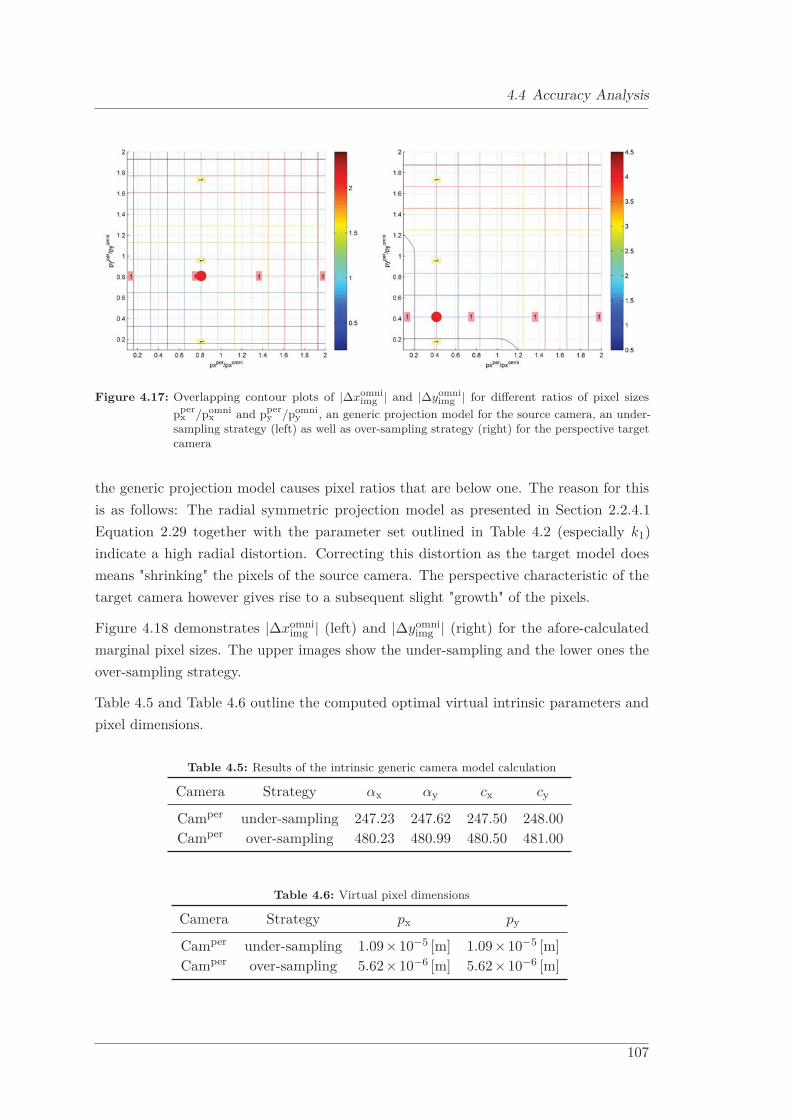
4.4 Accuracy Analysis
Figure 4.17: Overlapping contour plots of |Δxomniimg | and |Δyomni
img | for different ratios of pixel sizespper
x /pomnix and pper
y /pomniy , an generic projection model for the source camera, an under-
sampling strategy (left) as well as over-sampling strategy (right) for the perspective targetcamera
the generic projection model causes pixel ratios that are below one. The reason for thisis as follows: The radial symmetric projection model as presented in Section 2.2.4.1Equation 2.29 together with the parameter set outlined in Table 4.2 (especially k1)indicate a high radial distortion. Correcting this distortion as the target model doesmeans "shrinking" the pixels of the source camera. The perspective characteristic of thetarget camera however gives rise to a subsequent slight "growth" of the pixels.
Figure 4.18 demonstrates |Δxomniimg | (left) and |Δyomni
img | (right) for the afore-calculatedmarginal pixel sizes. The upper images show the under-sampling and the lower ones theover-sampling strategy.
Table 4.5 and Table 4.6 outline the computed optimal virtual intrinsic parameters andpixel dimensions.
Table 4.5: Results of the intrinsic generic camera model calculation
Camera Strategy αx αy cx cy
Camper under-sampling 247.23 247.62 247.50 248.00Camper over-sampling 480.23 480.99 480.50 481.00
Table 4.6: Virtual pixel dimensions
Camera Strategy px py
Camper under-sampling 1.09×10⁻⁵ [m] 1.09×10⁻⁵ [m]Camper over-sampling 5.62×10⁻⁶ [m] 5.62×10⁻⁶ [m]
107

4 Virtual Cameras
The values computed in the afore-presented example are only valid for this distinctconfiguration. They are crucially dependent on the underlying camera models (intrinsics)as well as their mutual extrinsic relationship, e.g. the rotation. The method can yet beapplied for all configurations and camera models.
Figure 4.18: Sample interval of the target image in the source image (left: x-direction, right: y-direction,top: under-sampling, bottom: over-sampling)
108

4.5 Performance Measurements
4.5 Performance Measurements
The previously described algorithm for virtual camera generation by (fast-) backwardmapping has been implemented in C++ as part of the professorships proprietary computervision framework. By employing the graphical interface of this framework, the user canparameterize the underlying functionality. So it is possible to do a live parameterizationof each individual perspective view. An impression is provided by Figure 4.19.
Figure 4.19: Live virtual camera generation [80]
The processing time for the conversion method was evaluated by means of eight LUTs ofdifferent sizes, described by the power of reduction n. The process, which was measured,consists of both the step for LUT generation together with the actual mapping procedurefrom the omnidirectional image to the perspective view. Two different resolutions ofthe target image were tested: 640 × 480 and 1280 × 960. The results are shown inFigure 4.20.
As it can be seen, the processing time declines rapidly with growing n. So the aimedspeed improvement in case of the optimized LUT calculation is confirmed. The fastestcalculation of the 640×480 sized target image is reached with n = 4 (processing time:8ms). After that, the Gauss-filtering consumes more time than the calculation of theLUT values. For the generation of a 1280 × 960 perspective image, this minimum islocated at n ≈ 5 (processing time: 33ms), because the initial LUT is 22 times larger thanthe initial one for a resolution of 640×480. So the optimal power of reduction dependson the desired size of the target image.
109
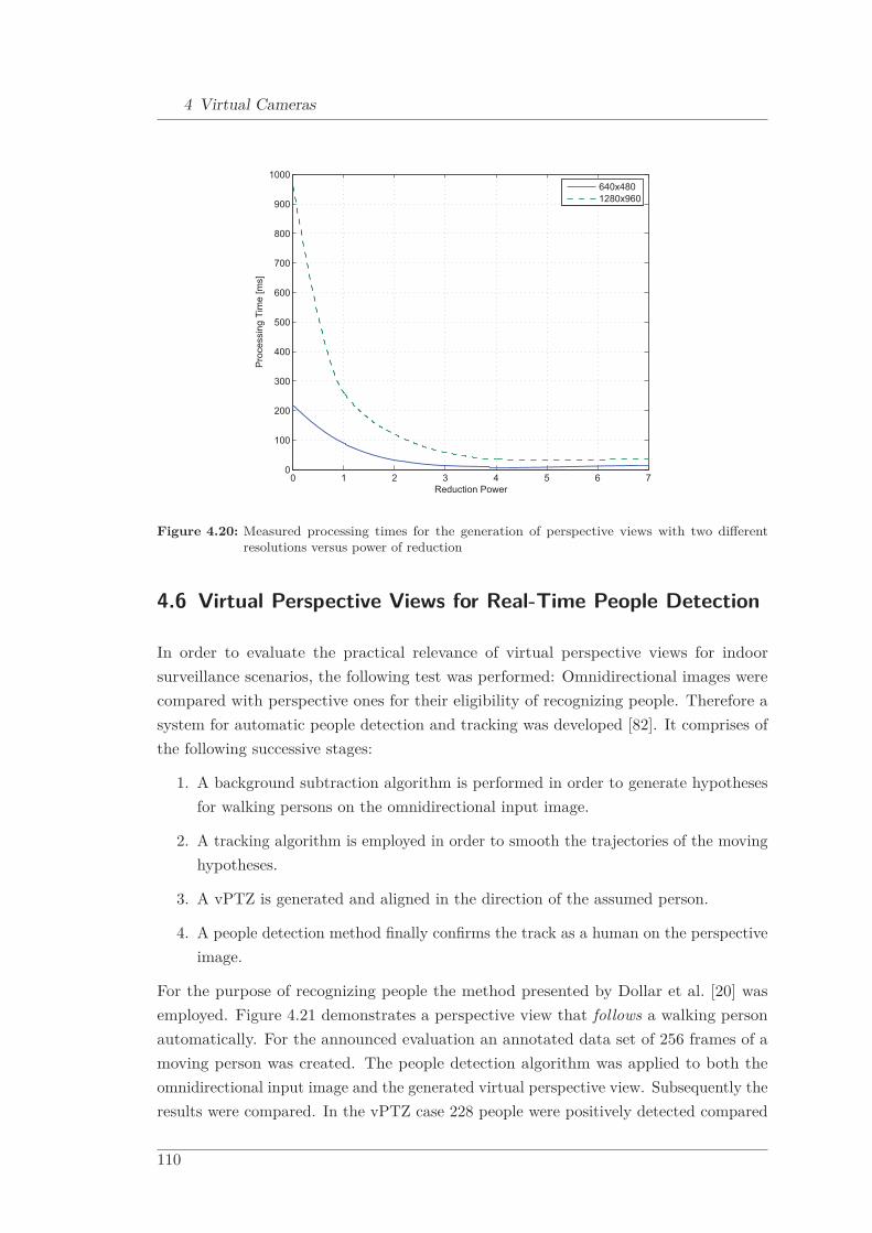
4 Virtual Cameras
0 1 2 3 4 5 6 70
100
200
300
400
500
600
700
800
900
1000
Reduction Power
Pro
cess
ing
Tim
e [m
s]
640x4801280x960
Figure 4.20: Measured processing times for the generation of perspective views with two differentresolutions versus power of reduction
4.6 Virtual Perspective Views for Real-Time People Detection
In order to evaluate the practical relevance of virtual perspective views for indoorsurveillance scenarios, the following test was performed: Omnidirectional images werecompared with perspective ones for their eligibility of recognizing people. Therefore asystem for automatic people detection and tracking was developed [82]. It comprises ofthe following successive stages:
1. A background subtraction algorithm is performed in order to generate hypothesesfor walking persons on the omnidirectional input image.
2. A tracking algorithm is employed in order to smooth the trajectories of the movinghypotheses.
3. A vPTZ is generated and aligned in the direction of the assumed person.
4. A people detection method finally confirms the track as a human on the perspectiveimage.
For the purpose of recognizing people the method presented by Dollar et al. [20] wasemployed. Figure 4.21 demonstrates a perspective view that follows a walking personautomatically. For the announced evaluation an annotated data set of 256 frames of amoving person was created. The people detection algorithm was applied to both theomnidirectional input image and the generated virtual perspective view. Subsequently theresults were compared. In the vPTZ case 228 people were positively detected compared
110

4.6 Virtual Perspective Views for Real-Time People Detection
Figure 4.21: Automatic people tracking system employing an omnidirectional imaging device and avPTZ [82]
to only 62 in the omnidirectional images. This corresponds to average detection ratesof 0.89 and 0.24 respectively. More precisely Figure 4.22 shows the spatial distributionof the detection rates in polar coordinates of the ground plane. The polar coordinatesystem consists of 32 angular bins and 5 radial bins. The maximum radius is 8m. Greenareas show high detection rates whereas red areas indicate poor detection rates. Whitespaces represent areas where no measurements were recorded.
Figure 4.22: Distribution of detection rates using an omnidirectional image directly (left) compared tothe use of virtual perspective views (right) [82]
Figure 4.22 visualizes that if a people detection algorithm is applied to the omnidirectionalimage directly, detection rates are only high when the person is visible in an upright (orupside down) position. By comparison the virtual perspective views produce consistentlyhigh detection rates for all positions. More details can be reviewed in the publication ofMeinel et al. [82].
111


Chapter 5
Omnidirectional Stereo Vision
This chapter presents and examines the idea of omnidirectional stereo vision which hasbeen motivated in Chapter 1. Therefore an extended overview about existing approachesis presented in Section 5.1. Especially the categorization of such systems with respect tothe geometrical camera configuration will be taken into focus and major derivatives arecompared. As stated in Chapter 3 parallel epipolar lines are a major precondition forstereo processing. Due to this, Section 5.2 outlines important rectification methods forthe afore-presented stereo configurations.
Based on the findings from Section 5.1 and Section 5.2, an idea for a novel omnidirectionalstereo vision setup is presented in Section 5.3.
5.1 Introduction and Related Works
The challenge of omnidirectional stereo vision has been discussed in several previousscientific publications. A comprehensive overview about the vast amount of approachescan be reviewed in the publication by Zhu [146].
A rough classification can be done by distinguishing strategies of image generation,different geometrical configurations, the achievable field of view, target applications and afew more as briefly explained in the following:
• Image generation: While special omnidirectional lens types can create a verywide-angle image, multiple ordinary perspective cameras have to be employed inorder to achieve this. Besides this static approach, moving imaging devices can beemployed to widen the FOV.
• Geometrical configurations: The number of used sensors as well as their mutualgeometrical alignment differ. This has a high impact on properties like FOV, staticor dynamic behaviour and type of sensor for instance.
113
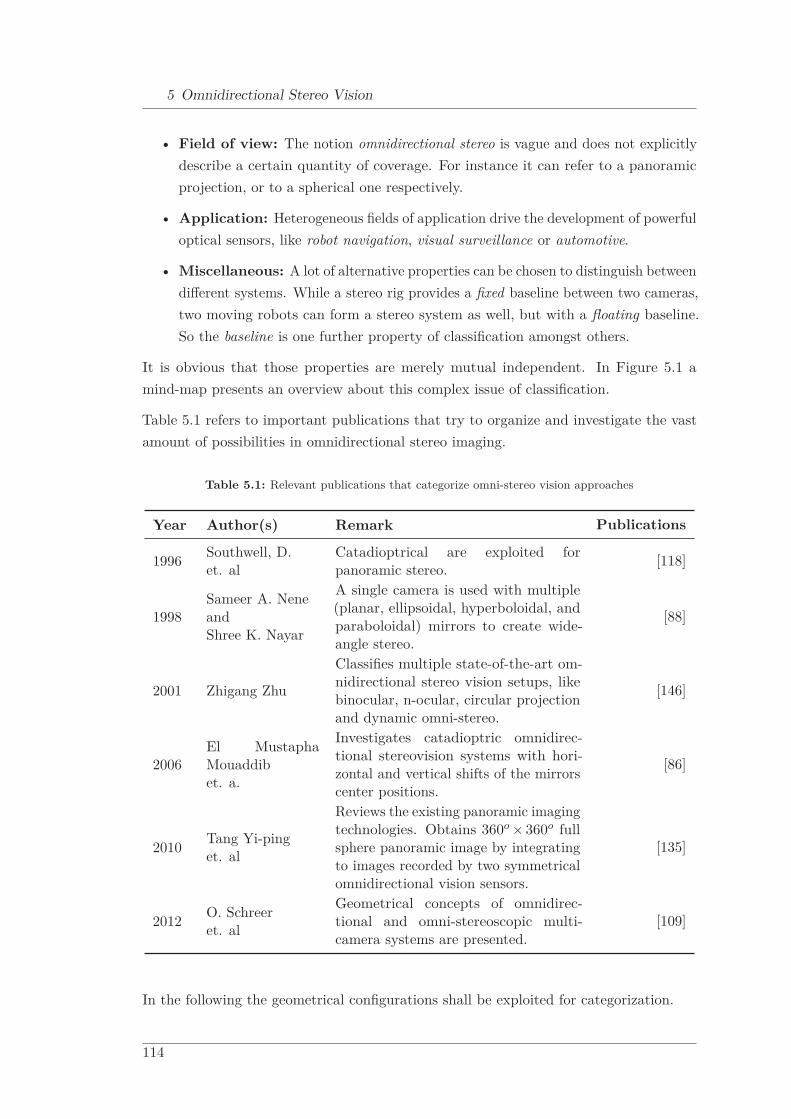
5 Omnidirectional Stereo Vision
• Field of view: The notion omnidirectional stereo is vague and does not explicitlydescribe a certain quantity of coverage. For instance it can refer to a panoramicprojection, or to a spherical one respectively.
• Application: Heterogeneous fields of application drive the development of powerfuloptical sensors, like robot navigation, visual surveillance or automotive.
• Miscellaneous: A lot of alternative properties can be chosen to distinguish betweendifferent systems. While a stereo rig provides a fixed baseline between two cameras,two moving robots can form a stereo system as well, but with a floating baseline.So the baseline is one further property of classification amongst others.
It is obvious that those properties are merely mutual independent. In Figure 5.1 amind-map presents an overview about this complex issue of classification.
Table 5.1 refers to important publications that try to organize and investigate the vastamount of possibilities in omnidirectional stereo imaging.
Table 5.1: Relevant publications that categorize omni-stereo vision approaches
Year Author(s) Remark Publications
1996 Southwell, D.et. al
Catadioptrical are exploited forpanoramic stereo. [118]
1998Sameer A. NeneandShree K. Nayar
A single camera is used with multiple(planar, ellipsoidal, hyperboloidal, andparaboloidal) mirrors to create wide-angle stereo.
[88]
2001 Zhigang Zhu
Classifies multiple state-of-the-art om-nidirectional stereo vision setups, likebinocular, n-ocular, circular projectionand dynamic omni-stereo.
[146]
2006El MustaphaMouaddibet. a.
Investigates catadioptric omnidirec-tional stereovision systems with hori-zontal and vertical shifts of the mirrorscenter positions.
[86]
2010 Tang Yi-pinget. al
Reviews the existing panoramic imagingtechnologies. Obtains 360o × 360o fullsphere panoramic image by integratingto images recorded by two symmetricalomnidirectional vision sensors.
[135]
2012 O. Schreeret. al
Geometrical concepts of omnidirec-tional and omni-stereoscopic multi-camera systems are presented.
[109]
In the following the geometrical configurations shall be exploited for categorization.
114

5.1 Introduction and Related Works
GeometricalConfiguration
,BinocularOmnistereo
,HorizontallyAligned
,VerticallyAligned
,HemisphericalStereo
,TrinocularOmnistereo
,N-OcularOmnistereo
,Circular ProjectionOmnistereo
(OmnivergentStereo),Dynamic
Omnistereo,Special Op-tical Solution
Image Generation
,OmnidirectionalCamera
,FisheyeLens
,Catadioptrical
,Image Mosaicing
,Full OpticalSolution
,TranslatingCameras
,RotatingCameras
,Center
,Off-Center
Field of View360o Azimuth
,180o
Elevation,90o Azimuth
,Perspective
Applications
,RobotNavigation
,3DRecon-
struction,Video
Surveillance
,Automotive
,Virtual Reality
,Cinema Miscellaneous
,Center
,ViewerCentered,Object
Centered
,Activeor
Passive
,Active
,Passive
,Baseline
,Fixed
,Floating
,View Points
,SingleView Point ,Multiple
View Points
Figure 5.1: Overview of categorizations for omni-stereo vision approaches
115
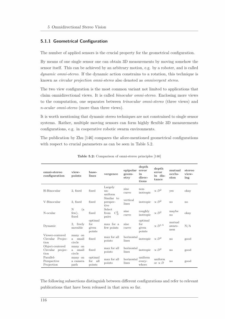
5 Omnidirectional Stereo Vision
5.1.1 Geometrical Configuration
The number of applied sensors is the crucial property for the geometrical configuration.
By means of one single sensor one can obtain 3D measurements by moving somehow thesensor itself. This can be achieved by an arbitrary motion, e.g. by a roboter, and is calleddynamic omni-stereo. If the dynamic action constrains to a rotation, this technique isknown as circular projection omni-stereo also denoted as omnivergent stereo.
The two view configuration is the most common variant not limited to applications thatclaim omnidirectional views. It is called binocular omni-stereo. Enclosing more viewsto the computation, one separates between trinocular omni-stereo (three views) andn-ocular omni-stereo (more than three views).
It is worth mentioning that dynamic stereo techniques are not constrained to single sensorsystems. Rather, multiple moving sensors can form highly flexible 3D measurementsconfigurations, e.g. in cooperative robotic swarm environments.
The publication by Zhu [146] compares the afore-mentioned geometrical configurationswith respect to crucial parameters as can be seen in Table 5.2.
Table 5.2: Comparison of omni-stereo principles [146]
omni-stereoconfiguration
view-points
base-lines vergence
epipolargeom-etry
deptherrorindirec-tions
deptherrorin dis-tance
mutualocclu-sion
stereoview-ing
H-Binocular 2, fixed fixedLargelyun-uniform
sinecurve
non-isotropic ∝ D2 yes okay
V-Binocular 2, fixed fixedSimilar toperspec-tive
verticallines isotropic ∝ D2 no no
N-ocularN (afew),fixed
fixedSelectfrom C2
Npairs
sinecurve
roughlyisotropic ∝ D2 maybe
no okay
Dynamic 2, freelymovable
optimalforgivenpoints
max for afew points
sinecurve
optimalforgivenpoints
∝ D1.5mutualaware-ness
N/A
Viewer-centeredCircular Projec-tion
many ona smallcircle
fixed max for allpoints
horizontallines isotropic ∝ D2 no good
Object-centeredCircular projec-tion
many ona smallcircle
fixed max for allpoints
horizontallines isotropic ∝ D2 no good
Parallel-PerspectiveProjection
many ona camerapath
optimalfor allpoints
max for allpoints
horizontallines
uniformevery-where
uniformor ∝ D
no good
The following subsections distinguish between different configurations and refer to relevantpublications that have been released in that area so far.
116

5.1 Introduction and Related Works
5.1.1.1 H-Binocular Omni-Stereo with Panoramic Views
Most binocular setups employ panoramic images that are a 360-degree cylindrical pro-jection from a single viewpoint where the projection in the vertical direction is perspec-tive [146]. Figure 5.2 shows a horizontally-aligned omni-stereo vision configuration wheretwo views are arranged in a horizontal setup with a fixed baseline.
Figure 5.2: H-binocular omni-stereo with panoramic views
This approach guarantees a horizontal panoramic 3D measurement field while the ob-servable FOV in vertical direction is constraint to common perspective projection charac-teristics.
According to a common stereo configuration as described in Section 3.5 a physical depthZ can be computed with respect to the left camera:
Z = b·sinφr
sin(φl −φr)= b·
sinφr
sin(φ)(5.1)
where
• b is the physical baseline between both sensors (see Section 2.4.1). [b] = mm
• φl is the angle of the left incoming ray on the principle plane (blue plane inFigure 5.2) with respect to the baseline (blue line in Figure 5.2) connecting thecentres of both imaging devices) . [φl] = rad
• φr is the angle of the right incoming ray on the principle plane (blue plane inFigure 5.2) with respect to the baseline (blue line in Figure 5.2) connecting thecentres of both imaging devices) . [φr] = rad
117

5 Omnidirectional Stereo Vision
• φ is the physical disparity φl −φr of the world point projections between left andright camera. [φ] = rad
According to Zhu [146] all epipolar curves are sinusoidal and a triangulation is not definedfor the singularity points when φl = φr = 0o. The obtained depth error is non-isotropic,proportional to the square of Z and inversely proportional to b. The latter fact iscongruent with perspective stereo.
A mentionable representative of the principle of horizontally-aligned omni-stereo waspresented by Kang et al. [52]. In their publication they compose cylindrical imagesfrom video sequences taken by vertically rotating cameras and recover 3-D point cloudsby structure from motion. For the computation of full 3D maps, they overcome theblind-spot problem by means of three sensors. A schematic configuration as presentedin [52] can be seen in Figure 5.3.
Figure 5.3: Example for horizontally-aligned omni-stereo [52]
Based on the results it can be concluded that the afore-presented method is not appropriatefor fast real-time stereo matching since the epipolar curves are not parallel straight lines.Rather they are sinusoidal. Standard methods for dense stereo computation cannot beapplied - it is more appropriate for approaches that triangulate sparse features. Thelimited vertical FOV makes it not very reasonable for indoor surveillance applications.
An overview about further related works with respect to this technology can be reviewedin Appendix B Table B.1.
118
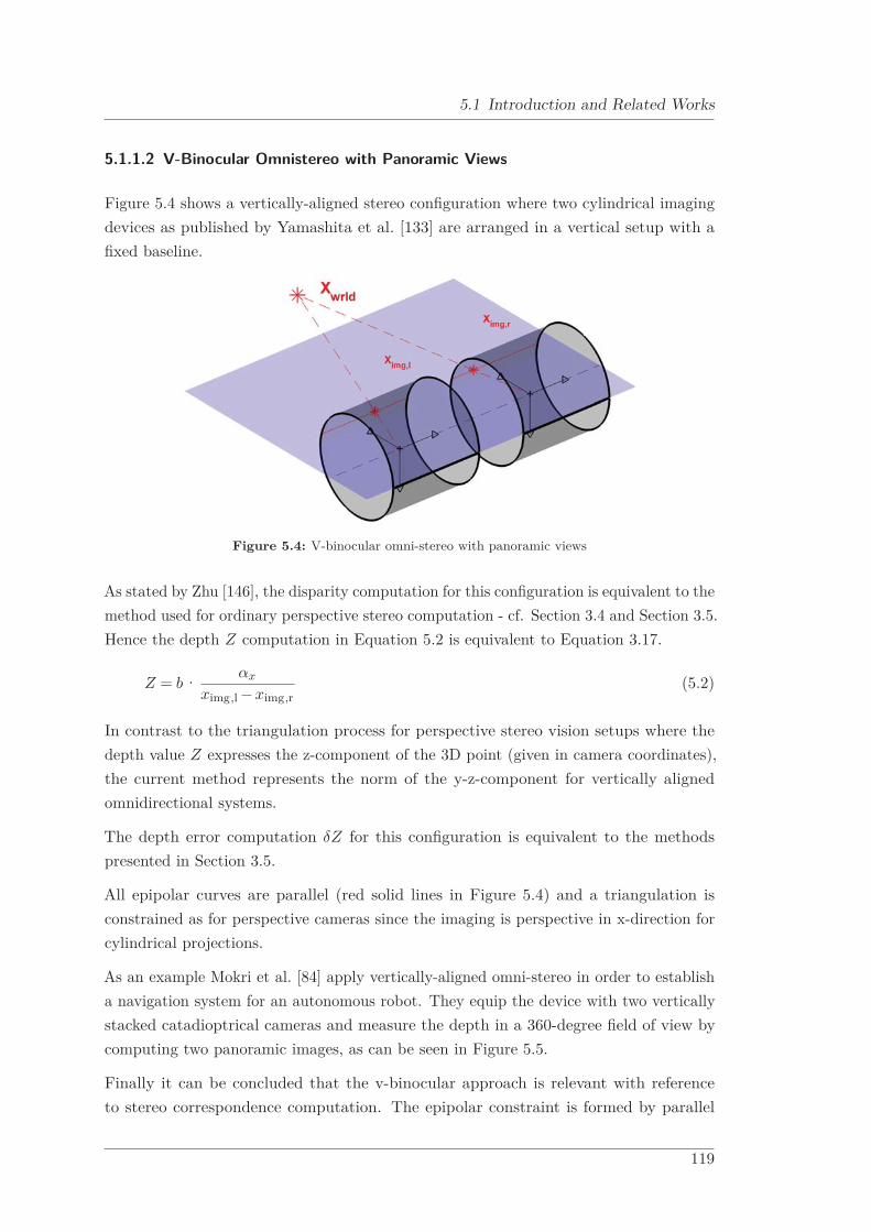
5.1 Introduction and Related Works
5.1.1.2 V-Binocular Omnistereo with Panoramic Views
Figure 5.4 shows a vertically-aligned stereo configuration where two cylindrical imagingdevices as published by Yamashita et al. [133] are arranged in a vertical setup with afixed baseline.
Figure 5.4: V-binocular omni-stereo with panoramic views
As stated by Zhu [146], the disparity computation for this configuration is equivalent to themethod used for ordinary perspective stereo computation - cf. Section 3.4 and Section 3.5.Hence the depth Z computation in Equation 5.2 is equivalent to Equation 3.17.
Z = b·αx
ximg,l −ximg,r(5.2)
In contrast to the triangulation process for perspective stereo vision setups where thedepth value Z expresses the z-component of the 3D point (given in camera coordinates),the current method represents the norm of the y-z-component for vertically alignedomnidirectional systems.
The depth error computation δZ for this configuration is equivalent to the methodspresented in Section 3.5.
All epipolar curves are parallel (red solid lines in Figure 5.4) and a triangulation isconstrained as for perspective cameras since the imaging is perspective in x-direction forcylindrical projections.
As an example Mokri et al. [84] apply vertically-aligned omni-stereo in order to establisha navigation system for an autonomous robot. They equip the device with two verticallystacked catadioptrical cameras and measure the depth in a 360-degree field of view bycomputing two panoramic images, as can be seen in Figure 5.5.
Finally it can be concluded that the v-binocular approach is relevant with referenceto stereo correspondence computation. The epipolar constraint is formed by parallel
119
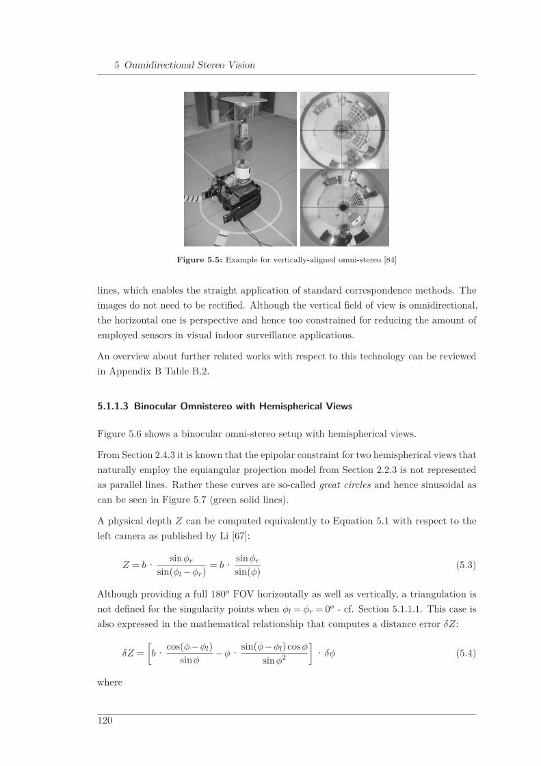
5 Omnidirectional Stereo Vision
Figure 5.5: Example for vertically-aligned omni-stereo [84]
lines, which enables the straight application of standard correspondence methods. Theimages do not need to be rectified. Although the vertical field of view is omnidirectional,the horizontal one is perspective and hence too constrained for reducing the amount ofemployed sensors in visual indoor surveillance applications.
An overview about further related works with respect to this technology can be reviewedin Appendix B Table B.2.
5.1.1.3 Binocular Omnistereo with Hemispherical Views
Figure 5.6 shows a binocular omni-stereo setup with hemispherical views.
From Section 2.4.3 it is known that the epipolar constraint for two hemispherical views thatnaturally employ the equiangular projection model from Section 2.2.3 is not representedas parallel lines. Rather these curves are so-called great circles and hence sinusoidal ascan be seen in Figure 5.7 (green solid lines).
A physical depth Z can be computed equivalently to Equation 5.1 with respect to theleft camera as published by Li [67]:
Z = b·sinφr
sin(φl −φr)= b·
sinφr
sin(φ)(5.3)
Although providing a full 180o FOV horizontally as well as vertically, a triangulation isnot defined for the singularity points when φl = φr = 0o - cf. Section 5.1.1.1. This case isalso expressed in the mathematical relationship that computes a distance error δZ:
δZ =[b·
cos(φ−φl)sinφ
−φ·sin(φ−φl)cosφ
sinφ2
]·δφ (5.4)
where
120

5.1 Introduction and Related Works
Figure 5.6: Binocular omni-stereo with hemispherical views
Ximg,l
φl
Ximg,rφr
Figure 5.7: Epipolar lines of binocular omni-stereo with hemispherical views
121

5 Omnidirectional Stereo Vision
• δφ is the accuracy a physical disparity can be determined with. [δφ] = rad
The closer φl gets to zero or π, and consequently the closer the point to triangulateapproaches the baseline (≡ the singularity points) - the more the measurement errorincreases. The smallest error is reached, when φl = π/2. Figure 5.8 plots qualitativelythe circumstances of Equation 5.4. The graphic visualizes the ascending error beginningat the most accurate value δZ up to 5·δZ. Beyond that value the error further headsfor infinity.
For applications that require a full hemispherical depth map, a two-view approach is notsufficient. This notion will be picked up again in Chapter 8.
Figure 5.8: Relationship between azimuth angle φl and qualitative error measurement δZ
As an example Zhu [145] applied the principles of binocular omni-stereo with two fish-eyesensors as can be seen in Figure 5.9. The physical projection process is approximated by aTaylor model. To overcome the challenge of non-parallel epipolar lines in omnidirectionalviews he employed a virtual perspective projection for rectification.
An overview about further related works with respect to this technology can be reviewedin Appendix B Table B.3.
5.1.1.4 Trinocular Omnistereo
As stated in Section 5.1.1.1, Section 5.1.1.2 and Section 5.1.1.3, binocular solutions aresubject to the drawback that a disparity is not defined for the singularity point. Li [67]overcomes this drawback by the application of a third camera. The configuration from
122
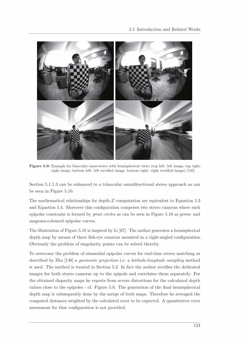
5.1 Introduction and Related Works
Figure 5.9: Example for binocular omni-stereo with hemispherical views (top left: left image, top right:right image, bottom left: left rectified image, bottom right: right rectified image) [145]
Section 5.1.1.3 can be enhanced to a trinocular omnidirectional stereo approach as canbe seen in Figure 5.10.
The mathematical relationships for depth-Z computation are equivalent to Equation 5.3and Equation 5.4. Moreover this configuration comprises two stereo cameras where eachepipolar constraint is formed by great circles as can be seen in Figure 5.10 as green- andmagenta-coloured epipolar curves.
The illustration of Figure 5.10 is inspired by Li [67]. The author generates a hemisphericaldepth map by means of three fish-eye cameras mounted in a right-angled configuration.Obviously the problem of singularity points can be solved thereby.
To overcome the problem of sinusoidal epipolar curves for real-time stereo matching asdescribed by Zhu [146] a gnomonic projection i.e. a latitude-longitude sampling methodis used. The method is treated in Section 5.2. In fact the author rectifies the dedicatedimages for both stereo cameras up to the epipols and correlates them separately. Forthe obtained disparity maps he reports from severe distortions for the calculated depthvalues close to the epipoles - cf. Figure 5.8. The generation of the final hemisphericaldepth map is subsequently done by the merge of both maps. Therefore he averaged thecomputed distances weighted by the calculated error to be expected. A quantitative errorassessment for that configuration is not provided.
123

5 Omnidirectional Stereo Vision
Figure 5.10: Trinocular omnidirectional stereo vision with hemispherical views
Figure 5.11: Example for trinocular omnidirectional stereo vision with hemispherical views [67]
124
5.1 Introduction and Related Works
An overview about further related works with respect to this technology can be reviewedin Appendix B Table B.4.
5.1.1.5 Miscellaneous Configurations
In addition to the afore-mentioned geometrical configurations, the principles of omnidi-rectional stereo have further been realized by means of alternative approaches. Althoughthose approaches are of less importance for this work, yet they shall be mentioned forcompleteness:
• N-ocular omnidirectional stereo vision - More than two or three views (n-ocular) are used extensively to improve the results of 3D measurements. Forinstance Sogo et al. [116] use several catadioptical sensors for real-time humantracking in order to tackle the correspondence problem amongst multiple targetsand thereby increase the measuring accuracy of target locations. An overview aboutfurther related works with respect to this technology can be seen in Appendix BTable B.5.
• Omnivergent stereo vision - Rotating single or multiple cameras around afixed axis realize so-called omnivergent stereo. Most approaches as publishedby Peleg [94–96] use ordinary perspective cameras in order to create panoramicprojections and hence panoramic stereo vision. An overview about further relatedworks with respect to this technology can be found in Appendix B Table B.6.
• Dynamic omnidirectional stereo vision - Creating 3D information by one ormultiple moving camera(s) is an established method in robotics. For instance Zhuet al. [147–149] generate dynamic panoramic stereo vision in a robot navigationscenario in order to find and protect humans by a robot team in an emergencycircumstance. They call this approach Panoramic Virtual Stereo Vision (PVS). Anoverview about further related works with respect to this technology can be viewedin Appendix B Table B.7.
• Omnidirectional stereo vision with special optical solutions - Besides thecommon imaging technologies based on perspective or omnidirectional (e.g. cata-dioptric and fisheye) optics, there exist multiple uncommon technologies. Anoverview about related works with respect to this technology can be reviewed inAppendix B Table B.8.
125
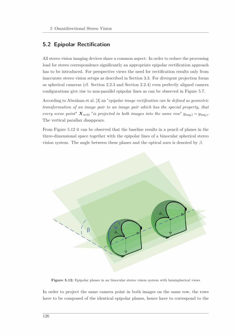
5 Omnidirectional Stereo Vision
5.2 Epipolar Rectification
All stereo vision imaging devices share a common aspect: In order to reduce the processingload for stereo correspondence significantly an appropriate epipolar rectification approachhas to be introduced. For perspective views the need for rectification results only frominaccurate stereo vision setups as described in Section 3.3. For divergent projection formsas spherical cameras (cf. Section 2.2.3 and Section 2.2.4) even perfectly aligned cameraconfigurations give rise to non-parallel epipolar lines as can be observed in Figure 5.7.
According to Abraham et al. [3] an "epipolar image rectification can be defined as geometrictransformation of an image pair to an image pair which has the special property, thatevery scene point" Xwrld "is projected in both images into the same row" yimg,l = yimg,r.The vertical parallax disappears.
From Figure 5.12 it can be observed that the baseline results in a pencil of planes in thethree-dimensional space together with the epipolar lines of a binocular spherical stereovision system. The angle between these planes and the optical axes is denoted by β.
Figure 5.12: Epipolar planes in an binocular stereo vision system with hemispherical views
In order to project the same camera point in both images on the same row, the rowshave to be composed of the identical epipolar planes, hence have to correspond to the
126
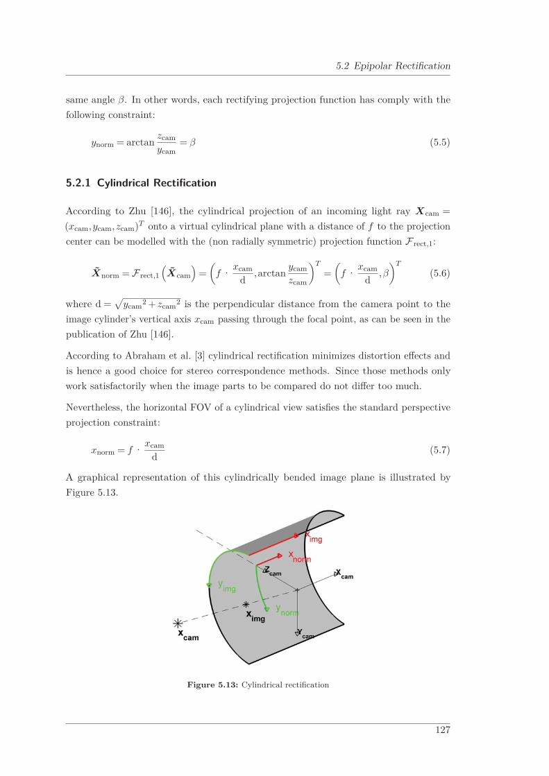
5.2 Epipolar Rectification
same angle β. In other words, each rectifying projection function has comply with thefollowing constraint:
ynorm = arctanzcam
ycam= β (5.5)
5.2.1 Cylindrical Rectification
According to Zhu [146], the cylindrical projection of an incoming light ray Xcam =(xcam,ycam,zcam)T onto a virtual cylindrical plane with a distance of f to the projectioncenter can be modelled with the (non radially symmetric) projection function F rect,1:
Xnorm = F rect,1(Xcam
)=
(f ·
xcam
d,arctan
ycam
zcam
)T
=(
f ·xcam
d,β
)T
(5.6)
where d =√
ycam2 +zcam2 is the perpendicular distance from the camera point to theimage cylinder’s vertical axis xcam passing through the focal point, as can be seen in thepublication of Zhu [146].
According to Abraham et al. [3] cylindrical rectification minimizes distortion effects andis hence a good choice for stereo correspondence methods. Since those methods onlywork satisfactorily when the image parts to be compared do not differ too much.
Nevertheless, the horizontal FOV of a cylindrical view satisfies the standard perspectiveprojection constraint:
xnorm = f ·xcam
d(5.7)
A graphical representation of this cylindrically bended image plane is illustrated byFigure 5.13.
Figure 5.13: Cylindrical rectification
127
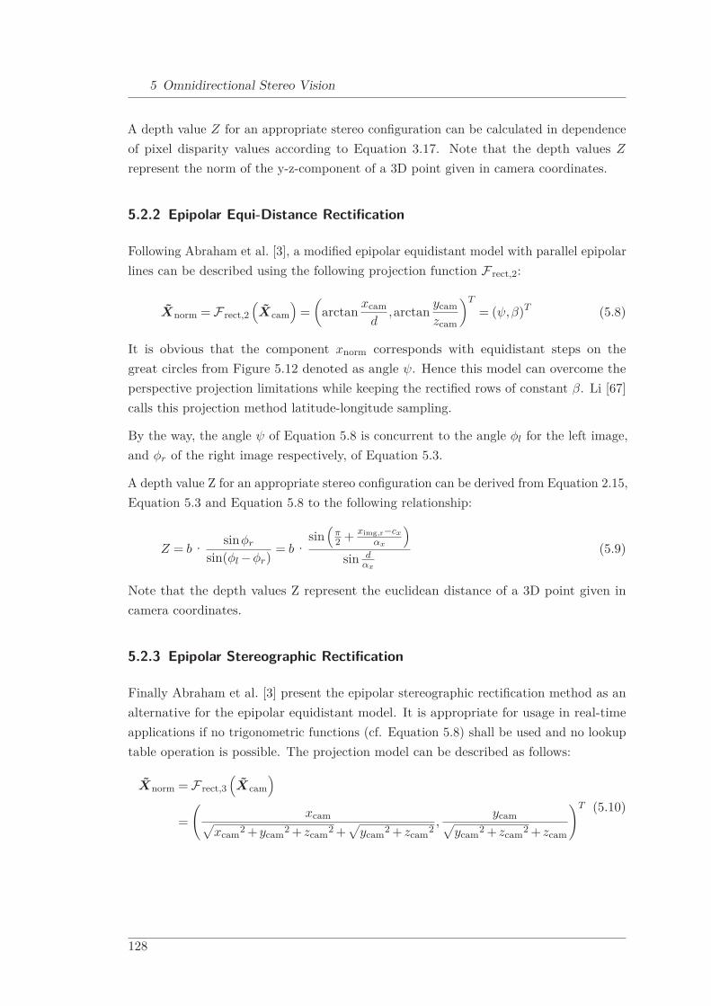
5 Omnidirectional Stereo Vision
A depth value Z for an appropriate stereo configuration can be calculated in dependenceof pixel disparity values according to Equation 3.17. Note that the depth values Z
represent the norm of the y-z-component of a 3D point given in camera coordinates.
5.2.2 Epipolar Equi-Distance Rectification
Following Abraham et al. [3], a modified epipolar equidistant model with parallel epipolarlines can be described using the following projection function F rect,2:
Xnorm = F rect,2(Xcam
)=
(arctan
xcam
d,arctan
ycam
zcam
)T
= (ψ,β)T (5.8)
It is obvious that the component xnorm corresponds with equidistant steps on thegreat circles from Figure 5.12 denoted as angle ψ. Hence this model can overcome theperspective projection limitations while keeping the rectified rows of constant β. Li [67]calls this projection method latitude-longitude sampling.
By the way, the angle ψ of Equation 5.8 is concurrent to the angle φl for the left image,and φr of the right image respectively, of Equation 5.3.
A depth value Z for an appropriate stereo configuration can be derived from Equation 2.15,Equation 5.3 and Equation 5.8 to the following relationship:
Z = b·sinφr
sin(φl −φr)= b·
sin(
π2 + ximg,r−cx
αx
)sin d
αx
(5.9)
Note that the depth values Z represent the euclidean distance of a 3D point given incamera coordinates.
5.2.3 Epipolar Stereographic Rectification
Finally Abraham et al. [3] present the epipolar stereographic rectification method as analternative for the epipolar equidistant model. It is appropriate for usage in real-timeapplications if no trigonometric functions (cf. Equation 5.8) shall be used and no lookuptable operation is possible. The projection model can be described as follows:
Xnorm = F rect,3(Xcam
)=
(xcam√
xcam2 +ycam2 +zcam2 +√
ycam2 +zcam2,
ycam√ycam2 +zcam2 +zcam
)T (5.10)
128
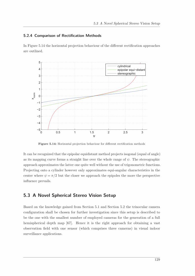
5.3 A Novel Spherical Stereo Vision Setup
5.2.4 Comparison of Rectification Methods
In Figure 5.14 the horizontal projection behaviour of the different rectification approachesare outlined.
0 0.5 1 1.5 2 2.5 3−5
−4
−3
−2
−1
0
1
2
3
4
5
ψ
x norm
cylindricalepipolar equi−distantstereographic
Figure 5.14: Horizontal projection behaviour for different rectification methods
It can be recognized that the epipolar equidistant method projects isogonal (equal of angle)as its mapping curve forms a straight line over the whole range of ψ. The stereographicapproach approximates the latter one quite well without the use of trigonometric functions.Projecting onto a cylinder however only approximates equi-angular characteristics in thecenter where ψ = π/2 but the closer we approach the epipoles the more the perspectiveinfluence prevails.
5.3 A Novel Spherical Stereo Vision Setup
Based on the knowledge gained from Section 5.1 and Section 5.2 the trinocular cameraconfiguration shall be chosen for further investigation since this setup is described tobe the one with the smallest number of employed cameras for the generation of a fullhemispherical depth map [67]. Hence it is the right approach for obtaining a vastobservation field with one sensor (which comprises three cameras) in visual indoorsurveillance applications.
129
5 Omnidirectional Stereo Vision
As disadvantageous for the algorithm described in Section 5.1.1.4 can be considered thattwo full-hemispherical depth maps of approximately original image size are calculatedwith both showing high inaccurate depth data near the epipoles:
• The rectification and subsequently the stereo processing of image data near theepipols lead to multiple redundant operations. For example if the rectified imagecomprises 1000 rows, the singularity pixel will be mapped to each of these linesduring epipolar equidistant rectification. After 1000 redundant stereo operationsthe obtained depth information is discarded in the merge stage.
• The weighted average method applied involves the computation of the actualdepth error for each pixel under consideration. Since this procedure includes thecalculation of multiple trigonometric functions (cf. Equation 5.4), it may not beappropriate for real-time processing.
• When a stereo sensor is designed, its error specification bases on the worst caseerror. Whatever the merge procedure of Li achieves, the worst case error valuecannot be more accurate than the best value of the binocular stereo vision setupwith hemispherical views - cf. Section 5.1.1.3 Figure 5.8. This is because in hissetup four singularities are included in the merge process - each time with thebest value from the complementary stereo camera. The question is now, whetheranother geometrical constellation and the employment of narrow-angled viewswithout complicated merge procedure may lead to the same result - at least nearly.
• If nothing else the right-angled trinocular stereo vision configuration as outlinedin Figure 5.11 is protected by at least U.S. patent claims1 which motivates toinvestigate an alternative approach in addition.
As basis for the further investigations I propagate the following hypotheses:
1. It is possible to apply an alternative three-view camera configuration compared toLi [67] in order to calculate a full-hemispherical depth map.
2. Using only narrow-angled views can avoid subsequent merging procedures of high-computational effort.
3. The avoidance of calculating unreliable depth information near the epipoles (thatis skipped during the merging process anyway) reduces the number of necessarystereo correspondence operations compared to Li [67].
The answers will be given in the following chapters. But let us start with a briefintroduction of the suggested configuration:
1 http://www.google.de/patents/USD445818
130
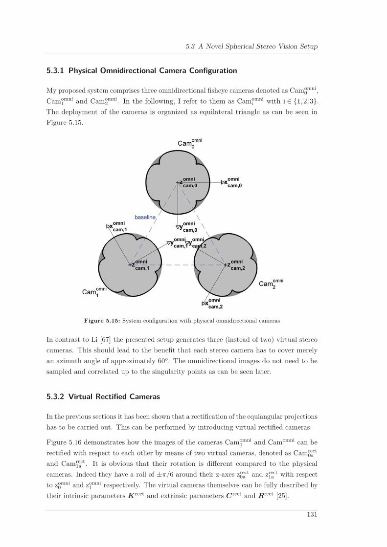
5.3 A Novel Spherical Stereo Vision Setup
5.3.1 Physical Omnidirectional Camera Configuration
My proposed system comprises three omnidirectional fisheye cameras denoted as Camomni0 ,
Camomni1 and Camomni
2 . In the following, I refer to them as Camomnii with i ∈ {1,2,3}.
The deployment of the cameras is organized as equilateral triangle as can be seen inFigure 5.15.
Figure 5.15: System configuration with physical omnidirectional cameras
In contrast to Li [67] the presented setup generates three (instead of two) virtual stereocameras. This should lead to the benefit that each stereo camera has to cover merelyan azimuth angle of approximately 60o. The omnidirectional images do not need to besampled and correlated up to the singularity points as can be seen later.
5.3.2 Virtual Rectified Cameras
In the previous sections it has been shown that a rectification of the equiangular projectionshas to be carried out. This can be performed by introducing virtual rectified cameras.
Figure 5.16 demonstrates how the images of the cameras Camomni0 and Camomni
1 can berectified with respect to each other by means of two virtual cameras, denoted as Camrect
0a
and Camrect1a . It is obvious that their rotation is different compared to the physical
cameras. Indeed they have a roll of ±π/6 around their z-axes zrect0a and zrect
1a with respectto zomni
0 and zomni1 respectively. The virtual cameras themselves can be fully described by
their intrinsic parameters Krect and extrinsic parameters Crect and Rrect [25].
131

5 Omnidirectional Stereo Vision
Camrect0a and Camrect
1a form together a virtual stereo camera denoted as SCamrecta ∈{
Camrect0a ,Camrect
1a}.
Figure 5.16: System configuration with two virtual rectified cameras
In order to exploit the geometrical setup to the whole extent, it is equipped with sixvirtual rectified cameras denoted as Camrect
0a , Camrect0b , Camrect
1a , Camrect1c , Camrect
2b andCamrect
2c , or Camrectj with j ∈ {0a,0b,1a,1c,2b,2c} respectively. Together these virtual
views generate three stereo cameras SCcamrecta ,SCamrect
b ,SCamrectc , or SCcamrect
k withk ∈ {a,b,c} respectively. This is summarized in Equation 5.11.
SCamrecta = {Camrect
0a ,Camrect1a }
SCamrectb = {Camrect
2b ,Camrect0b }
SCamrectc = {Camrect
1c ,Camrect2c }
(5.11)
Figure 5.17 shows the complete configuration of three physical cameras (black) togetherwith six virtual rectified views organized in three pairs (red, green and blue).
In principle each method for rectification that has been presented in Section 5.2 couldpossibly be used for this configuration, because a full rectification of the spherical imagesis not necessary. Since the epipolar equidistant method has been successfully applied byLi [67] and the cylindrical method is predestined for stereo correspondence processing asstated by Abraham et al. [3], I will continue the feasibility study by comparing both. Areal-time implementation as can be done by means of epipolar stereographic rectificationis not yet the major concern of this investigation. Since the latter method shows almostidentical projection behaviour compared to the epipolar equidistant principle, its explicittreatment is skipped for the time being.
In the following chapter the hereby presented configuration will be exploited in order togenerate a full hemispherical depth map.
132

5.3 A Novel Spherical Stereo Vision Setup
Figure 5.17: System configuration with six virtual rectified cameras
133


Chapter 6
A Novel Spherical Stereo VisionAlgorithm
The concept of a novel three-view camera setup as presented in Section 5.3 shall be usedin this chapter for the generation of a full hemispherical depth map.
It starts with introducing a MATLAB® simulation environment in Section 6.1. Thecamera deployment as well as its intrinsic parametrization is explained in Section 6.2,Section 6.3 and Section 6.4. Successively based on the simulation setup the depth mapcomputation is performed in Section 6.5. Finally an error estimation is presented inSection 6.6.
The basic idea as presented in Chapter 6 has been published by the author in scientificpublications [23,24].
6.1 Matlab Simulation Environment
For the purpose of simulation and evaluation of the novel spherical stereo vision algorithm,a reproducible data set shall be utilized. Therefore a MATLAB® test environment providesvirtual 3D data of an exemplary domestic environment.
A single artificial room of the size of 5m×5m×2.5m is presented in Figure 6.1. Mathe-matically it forms a quantity of scattered world points Xwrld.
The physical omnidirectional imaging devices Camomni0 , Camomni
1 and Camomni2 are in-
dicated by their coordinate systems (red, green and blue). Since Camomni0 represents
the reference camera in the stereo vision system with respect to the other cameras, it islocated at the ceiling in the middle of the virtual room.
135

6 A Novel Spherical Stereo Vision Algorithm
To form the scenario realistic and comparable, different configurations of the omnidirec-tional stereo setup will be simulated.
Figure 6.1: Virtual 3D test environment equipped with a spherical stereo vision sensor
6.2 Extrinsic Configuration
The general deployment of Camomnii and Camrect
j has been introductorily outlined in Sec-tion 5.3. Now the cameras shall be parametrized realistically. Therefore two configurationswith different baselengths will be investigated: b = 10cm and b = 15cm.
Initially Comni0 is determined to be the origin of the world coordinate system, i.e. we
define Romni0 = I and Comni
0 = 0. Since all physical cameras are to form an equilateraltriangle and shall have a mutual differential rotation of pi/2, one can calculate the cameraorigins Comni
i , the rotation matrices Romnii and consequently the translation vectors
T omnii by following the mathematics of Section 2.2.1.3.
The virtual cameras Camrectj have the identical origins Crect
j as their correspondingphysical equivalent. However, in order to achieve the configuration of Section 5.3.2 thecameras Camrect
j are rotated by ±pi/6 around their z-axis. Subsequently, they obtainnew rotation matrices and Rrect
j and translation vectors T rectj .
136

6.3 Physical Camera Configuration
6.3 Physical Camera Configuration
While an ideal omnidirectional camera obeys the equiangular projection principle aspresented in Section 2.2.3, real devices can better be described using the generic modelof Section 2.2.4. In the following both variants shall be considered.
Further parameters will orientate towards the industry camera of Section 4.4.1 having aresolution (height×width) of 1680×1680 with a focal length of f = 2.7mm. The intrinsicparameters already presented in Table 4.2 and Table 4.3 shall be used for example.
The parameters of the equiangular model can be calculated as follows: It is intended toobserve a FOV of 180◦ in horizontal and vertical direction exploiting the full pixel range.Hence the pixel densities can be computed as mx = width/(f ·π) = (2·cx)/(f ·π) andmy = height/(f ·π) = (2·cy)/(f ·π) where cx and cy are the horizontal and verticaloffset values of the principal point from the pixel frame - cf. Section 2.2.1.2. The obtainedintrinsic parameters can be seen in Table 6.1 and Table 6.2.
Table 6.1: Intrinsic parameters of the equiangular cameras Camomnii
Camera Projection Model αx αy cx cy
Camomnii Equiangular 534.76 534.76 840.50 840.50
Table 6.2: Physical pixel dimensions of the equiangular cameras Camomnii
Camera Projection Model px py
Camomnii Equiangular 5.05×10⁻⁶ [m] 5.05×10⁻⁶ [m]
Using the mathematical relation of Equation 2.16 described in Section 2.2.1.2 in com-bination with the afore-computed intrinsic values, an intrinsic matrix Komni
i can beestablished for each physical camera and each configuration.
6.4 Virtual Camera Configuration
In Section 5.3 the general deployment of the virtual cameras (extrinsic parameters) hasbeen discussed. The crucial issue is now to investigate what intrinsic parameters areappropriate for covering the whole environment. As a result of Chapter 4 a sensibleresolution of a virtual target camera highly depends on the underlying physical resolutionof the source camera. Furthermore in Chapter 3 the impact of the (virtual) stereo camerasresolution on the 3D measurement accuracy has been stated. A suggestion for derivingvirtual camera parameters is given in the following subsections.
137

6 A Novel Spherical Stereo Vision Algorithm
6.4.1 The Focal Length
The focal length f can be chosen freely and is determined to f = 2.7mm in analogy toSection 6.3. Setting an identical focal length of source and target camera makes theunderlying pixel sizes directly comparable since they scale proportional to f .
6.4.2 Prediscussion of the Field of View
According to Section 5.3 each virtual stereo camera SCamrectk has to cover a minimum
horizontal field of view FOVh of 60o and a vertical field of view FOVv of 180o for ahemispherical scene coverage.
All rectification methods presented in Section 5.2 are characterized by an equiangularbehaviour in vertical direction. Equation 6.1 shows that FOVv for the equiangular modelcan be calculated in dependence of the vertical resolution of the image and a given virtualpixel height py. In other words: With a given field of view a predefined pixel height isrequired in order to determine the vertical number of pixels (height).
FOVv =2·cy −1
αy=
height·py
f(6.1)
The afore-presented rectification methods of Section 5.2 show different horizontal pro-jection behaviour: While the cylindrical method rectifies perspectively, the epipolarequidistance method performs this operation equiangular. The following equationsdemonstrate the calculation of FOVh for both approaches - cylindrical (Equation 6.2)and epipolar equidistance (Equation 6.3) rectification:
FOVh = 2· arctan(2·cy −1
2·αx
)= 2· arctan
(width·px
2·f
)(6.2)
FOVh =2·cx −1
αx=
width·px
f(6.3)
Both can be computed in dependence of the horizontal resolution of the image and agiven virtual pixel width px (cf. Equation 4.11). I.e. with a given FOV a predefinedpixel width is required to determine the horizontal number of pixels.
In addition Section 3.5.2 discussed that the horizontal field of view FOVh of the virtualstereo cameras SCamrect
k cannot be identical to the FOVh of Camrectj . A maximal
measurable disparity dmax (depending on a configurable minimal measurable depthZmin and the baseline b) together with the pixel length px reduce the actual observablehorizontal area.
138
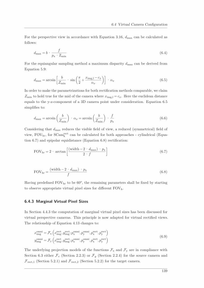
6.4 Virtual Camera Configuration
For the perspective view in accordance with Equation 3.16, dmax can be calculated asfollows:
dmax = b·f
px ·Zmin(6.4)
For the equiangular sampling method a maximum disparity dmax can be derived fromEquation 5.9:
dmax = arcsin[
b
Zmin· sin
(π
2+
ximg,l − cx
αx
)]·αx (6.5)
In order to make the parametrizations for both rectification methods comparable, we claimZmin to hold true for the mid of the camera where ximg,l = cx. Here the euclidean distanceequals to the y-z-component of a 3D camera point under consideration. Equation 6.5simplifies to:
dmax = arcsin(
b
Zmin
)·αx = arcsin
(b
Zmin
)·
f
px(6.6)
Considering that dmax reduces the visible field of view, a reduced (symmetrical) field ofview, FOVhr, for SCamrect
k can be calculated for both approaches - cylindrical (Equa-tion 6.7) and epipolar equidistance (Equation 6.8) rectification:
FOVhr = 2· arctan[(width −2·dmax) ·px
2·f
](6.7)
FOVhr =(width −2·dmax) ·px
f(6.8)
Having predefined FOVhr to be 60o, the remaining parameters shall be fixed by startingto observe appropriate virtual pixel sizes for different FOVh.
6.4.3 Marginal Virtual Pixel Sizes
In Section 4.4.3 the computation of marginal virtual pixel sizes has been discussed forvirtual perspective cameras. This principle is now adapted for virtual rectified views.The relationship of Equation 4.13 changes to:
xomniimg = Fx
(xrect
img ,yrectimg ;pomni
x ,pomniy ,prect
x ,precty
)yomni
img = Fy(xrect
img ,yrectimg ;pomni
x ,pomniy ,prect
x ,precty
) (6.9)
The underlying projection models of the functions Fx and Fy are in compliance withSection 6.3 either Fe (Section 2.2.3) or Fg (Section 2.2.4) for the source camera andF rect,1 (Section 5.2.1) and F rect,2 (Section 5.2.2) for the target camera.
139

6 A Novel Spherical Stereo Vision Algorithm
Based on Section 4.4.3 we can determine the virtual pixel size according to the under-sampling as well as over-sampling strategy. Since reliable depth measurements by stereocomputation base on virtual pixel information that is substantiated by underlying physicalpixels appropriately, only the under-sampling method shall be further considered. Theactual computation can now be performed by evaluating the following mathematicalexpression:
minimize(||∇Fx|−1.0|+ ||∇Fy|−1.0|) (6.10)
This evaluation has been performed for all projection models under consideration inter-changeably. A virtual camera which is fed by the physical one is simulated with its rotatedorientation (more precisely a roll of ±π/6 around its z-axis as shown in Section 5.3.2), aFOVv of 180o and a varying FOVh between 60o and 90o:
• FOVh = 60o: This is the theoretical minimum in the presented approach which hasto be covered by each virtual stereo camera SCamrect
k and hence by each virtualcamera Camrect
j .
• FOVh = 90o: This is the theoretical minimum in the approach presented by Li [67]which has to be covered by each of both stereo cameras.
In order to solve this problem numerically for each FOVh between 60o and 90o, a rangeof pixel size ratios prect
x /pomnix and prect
y /pomniy has been investigated in order to feed
Equation 6.10. The distinct value range originates from results of Chapter 4 and isoutlined in Equation 6.11:
prectx /pomni
x ∈ [0.25,2.50]
precty /pomni
y ∈ [0.25,2.50](6.11)
The pixel coordinates xrectimg and yrect
img , which are further parameters for Equation 6.10 arecalculated by Equation 6.1, Equation 6.2 and Equation 6.3:
xrectimg ∈ [0,width −1]
yrectimg ∈ [0,height−1]
(6.12)
In accordance with Figure 4.17 of Section 4.4.3 one can observe overlapping contourplots of |Δxomni
img | and |Δyomniimg | for two exemplary configurations in Figure 6.2. It can be
observed that the optimal pixel ratios indicated by red dots differ for each configuration.One can state that the more the horizontal field of view increases the more the obtainedresolution for the virtual (cylindrical) camera decreases in horizontal as well as verticaldirection. In other words: The size of the virtual pixels prect
x and precty grows with an
increasing horizontal field of view.
140

6.4 Virtual Camera Configuration
Figure 6.2: Overlapping contour plots of |Δxomniimg | and |Δyomni
img | for different ratios of pixel sizesprect
x /pomnix and prect
y /pomniy , an equiangular projection model for the source camera, a
cylindrical projection model for the target camera, an under-sampling strategy and FOVh =60o (left) and FOVh = 90o (right)
Figure 6.3 demonstrates how the sampling interval of the source images x-direction|Δxomni
img | (left plot) and the source images y-direction |Δyomniimg | (right plot) deploys over
the target image for the exemplary configuration of FOVh = 60o. The outer dark bluecoded areas specify the actual virtual pixel size since its sampling interval coincides withthe physical one. The red areas indicate high under-sampling.
Remark: Figure 6.3 visualizes the roll of +π/6 of the target camera in comparison tothe source camera. For the alternative roll of −π/6, Equation 6.10 shows symmetricalbehaviour.
In Figure 6.4 the optimal pixel ratios for each configuration can be observed dependingon the different FOVh. The optimal virtual pixel size becomes a function f of the physicalpixel size and the field of view:
prectx = f
(pomni
x ,FOVh)
precty = f
(pomni
y ,FOVh) (6.13)
Equally to Section 4.4 one can see that a source camera following the generic projectionmodel (blue and cyan graphs) causes pixel ratios that are below one - in comparisonto the equiangular model (red and green graphs). It is interesting to discover that theoptimal pixel ratios prect
x /pomnix in horizontal direction strongly grow for the cylindrical
model (red and blue graphs, left chart) with the increase of FOVh while prectx /pomni
x onlyslightly change for the epipolar equidistant projection principle. However, for the verticaldirection prect
y /pomniy both rectification models behave identically.
141

6 A Novel Spherical Stereo Vision Algorithm
Figure 6.3: Colour coded sampling interval |Δxomniimg | (left) and |Δyomni
img | (right) for the optimal pixelratios pcyl
x /pomnix and pcyl
y /pomniy , an equiangular projection model for the source camera,
a cylindrical projection model for the target camera, an under-sampling strategy andFOVh = 60o
6.4.4 Calculation of the Field of View
Combining Equation 6.3 and Equation 6.4 with Equation 6.13 the disparity range dmax
can be calculated for both target models depending on different FOVh and the underlyingphysical pixel size pomni
x - parametrized by a predefined minimal measurable depth Zmin.Assuming the sensor to be mounted 2.50m over ground and a person to be of 1.75m
height, a suitable exemplary Zmin shall be defined to be 0.75m. Equation 6.14 andEquation 6.15 outline the calculation of dmax for cylindrical (Equation 6.14) and epipolarequidistance (Equation 6.15) projection:
dmax = b·f
prectx ·Zmin
= b·f
f (pomnix ,FOVh) ·Zmin
(6.14)
dmax = arcsin(
b
Zmin
)·
f
prectx
= arcsin(
b
Zmin
)·
f
f (pomnix ,FOVh)
(6.15)
Figure 6.5 presents the simulation results for the afore-discussed configurations underconsideration.
Figure 6.5 demonstrates the impact of FOVh on dmax. For the cylindrical rectificationmethod the disparity range rapidly diminishes because the underlying pixel size increasessignificantly - as shown in Figure 6.4. For the epipolar equidistant approach, dmax changesonly slightly.
142

6.4 Virtual Camera Configuration
With a given maximum disparity range dmax and a given virtual pixel size prectx , both
depending on FOVh, the reduced field of view FOVhr can be computed depending onFOVh as well, according to Equation 6.5 and Equation 6.7. The results are presented inFigure 6.6.
It has turned out that the computation of the reduced field of field FOVhr that alreadyincludes the stereo disparity range pixel trade-off based on FOVh only depends on thebaselength b and the target rectification model. For a given minimum FOVhr = 60o theminimum FOVh can be easily extracted from Figure 6.6 and is summarized in Table 6.3.
Table 6.3: Calculated fields of view FOVh for the virtual cameras Camrectj according to the variety of
configurations
No. Camomnii Camrect
j b [m] FOVhr [deg] Zmin [m] FOVh [deg]
1 equiangular cylindrical 0.10 60.0 0.75 70.902 equiangular cylindrical 0.15 60.0 0.75 75.803 kannala9 cylindrical 0.10 60.0 0.75 70.904 kannala9 cylindrical 0.15 60.0 0.75 75.805 equiangular epipolar equidistance 0.10 60.0 0.75 75.406 equiangular epipolar equidistance 0.15 60.0 0.75 83.207 kannala9 epipolar equidistance 0.10 60.0 0.75 75.408 kannala9 epipolar equidistance 0.15 60.0 0.75 83.20
6.4.5 Calculation of the Virtual Pixel Size Ratios
Having determined FOVh for each configuration, the appropriate virtual pixel sizeratios can be extracted from Figure 6.4. The virtual image sizes are calculated usingEquation 6.1, Equation 6.2 and Equation 6.3. Table 6.4 summarizes the results.
Table 6.4: Calculated virtual pixel size ratios and image sizes
No. FOVh [deg] prectx /pomni
x precty /pomni
y height width dmax
1 70.90 1.5060 1.2195 1377 505 482 75.80 1.6120 1.2526 1341 516 673 70.90 0.6223 0.4908 1283 458 434 75.80 0.6632 0.5024 1254 470 615 75.40 1.0064 1.2498 1344 699 726 83.20 1.0176 1.3065 1285 763 1067 75.40 0.4140 0.5022 1254 636 658 83.20 0.4140 0.5246 1201 702 98
143

6 A Novel Spherical Stereo Vision Algorithm
6.4.6 Results of the Virtual Camera Parameters
As shown in Section 2.2.1.2 the given information can now be employed to obtain theintrinsic parameters by applying the fundamentals presented in Section 2.2.1. The resultsare outlined in Table 6.5 and Table 6.6. Using the relations described in Section 2.2.1.2
Table 6.5: Intrinsic parameters of the virtual cameras Camrectj
No. Camera αx αy cx cy
1 Camrectj 355.09 438.51 253.00 689.00
2 Camrectj 331.74 426.92 258.50 671.00
3 Camrectj 321.80 408.67 229.50 642.00
4 Camrectj 301.95 399.23 235.50 627.50
5 Camrectj 531.36 427.88 350.00 672.50
6 Camrectj 525.51 409.31 382.00 643.00
7 Camrectj 483.71 399.39 318.50 627.50
8 Camrectj 483.71 382.34 351.50 601.00
and the afore-computed intrinsic values, an intrinsic matrix Krectj can be established for
each virtual camera and each configuration.
Table 6.6: Pixel dimensions of the virtual cameras Camrectj
No. Camera px[m] py[m]
1 Camrectj 7.60×10⁻⁶ 6.16×10⁻⁶
2 Camrectj 8.14×10⁻⁶ 6.32×10⁻⁶
3 Camrectj 8.39×10⁻⁶ 6.61×10⁻⁶
4 Camrectj 8.94×10⁻⁶ 6.76×10⁻⁶
5 Camrectj 5.08×10⁻⁶ 6.31×10⁻⁶
6 Camrectj 5.14×10⁻⁶ 6.60×10⁻⁶
7 Camrectj 5.58×10⁻⁶ 6.76×10⁻⁶
8 Camrectj 5.58×10⁻⁶ 7.06×10⁻⁶
From Table 6.6 it becomes visible that the epipolar equidistant method produces higherresolutive target images compared to a cylindrical projection, which allows more accuratedepth measurements. Since this approach clearly outperforms the cylindrical rectificationit will be the rectification method of choice for further investigations.
144
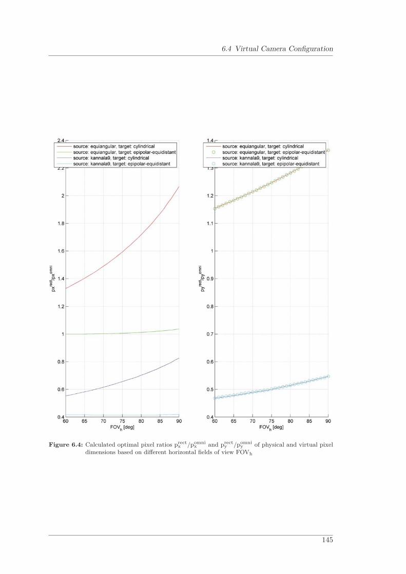
6.4 Virtual Camera Configuration
Figure 6.4: Calculated optimal pixel ratios prectx /pomni
x and precty /pomni
y of physical and virtual pixeldimensions based on different horizontal fields of view FOVh
145
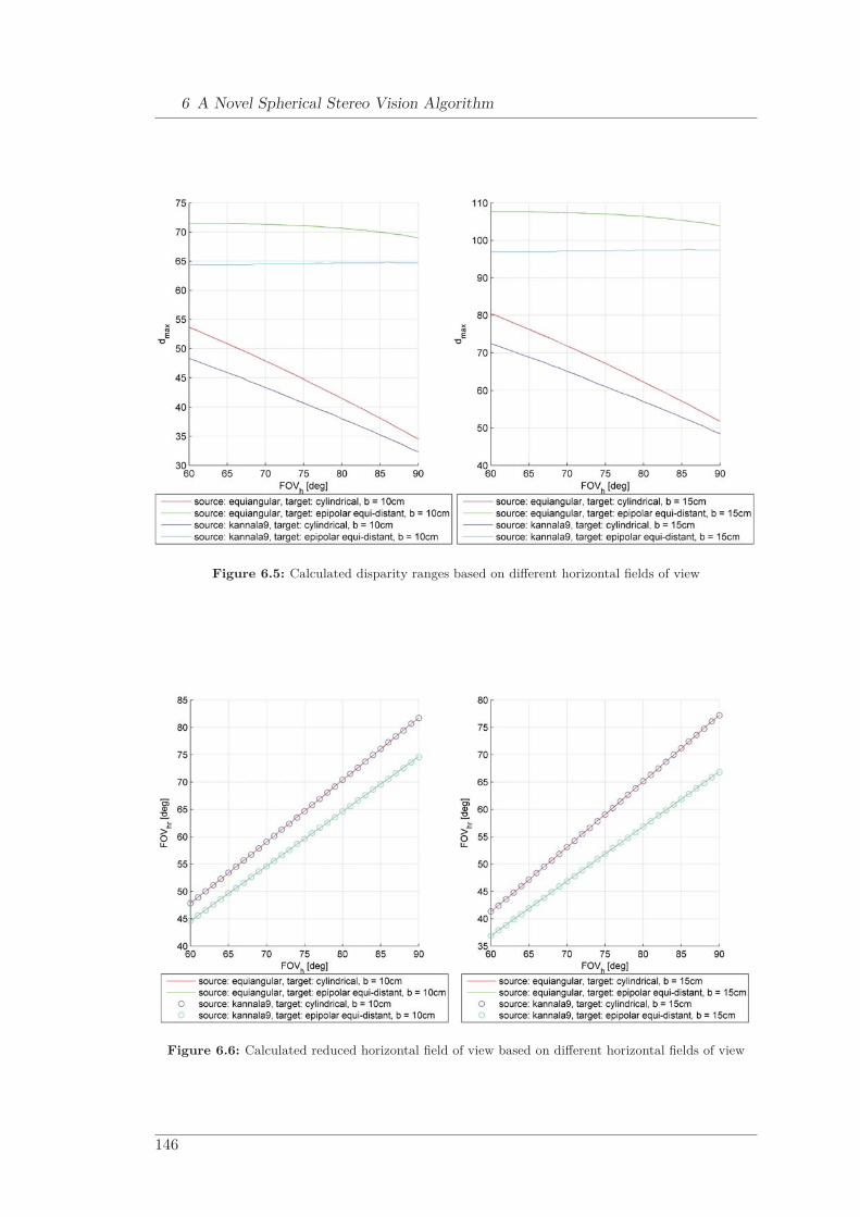
6 A Novel Spherical Stereo Vision Algorithm
Figure 6.5: Calculated disparity ranges based on different horizontal fields of view
Figure 6.6: Calculated reduced horizontal field of view based on different horizontal fields of view
146

6.5 Spherical Depth Map Generation
6.5 Spherical Depth Map Generation
The experimental setup from Section 6.1 together with the parametrizations of Section 6.5and Section 6.6 are now employed to generate a spherical depth map Zomni
0 that refers toCamomni
0 . The precondition for this simulation is the consideration of the scene itself asa quantity of scattered 3D world points Xwrld. The complete algorithm is summarizedin Figure 6.7.
Observed Scene Xwrld
ImagingCamomni
1
ImagingCamomni
0
ImagingCamomni
2
Image Iomni1Image Iomni
0 Image Iomni2
ImagingCamrect
0a
ImagingCamrect
0b
ImagingCamrect
1c
ImagingCamrect
1a
ImagingCamrect
2b
ImagingCamrect
2c
ImageIrect
0a
ImageIrect
0b
ImageIrect
1a
ImageIrect
1c
ImageIrect
2b
ImageIrect
2c
StereoCorre-
spondenceSCamrect
a
StereoCorre-
spondenceSCamrect
c
StereoCorre-
spondenceSCamrect
b
DepthZrect
0a
DepthZrect
1c
DepthZrect
2b
Depth Map Merge
Depth Zomni0
Figure 6.7: Summary of the spherical depth map generation algorithm
147
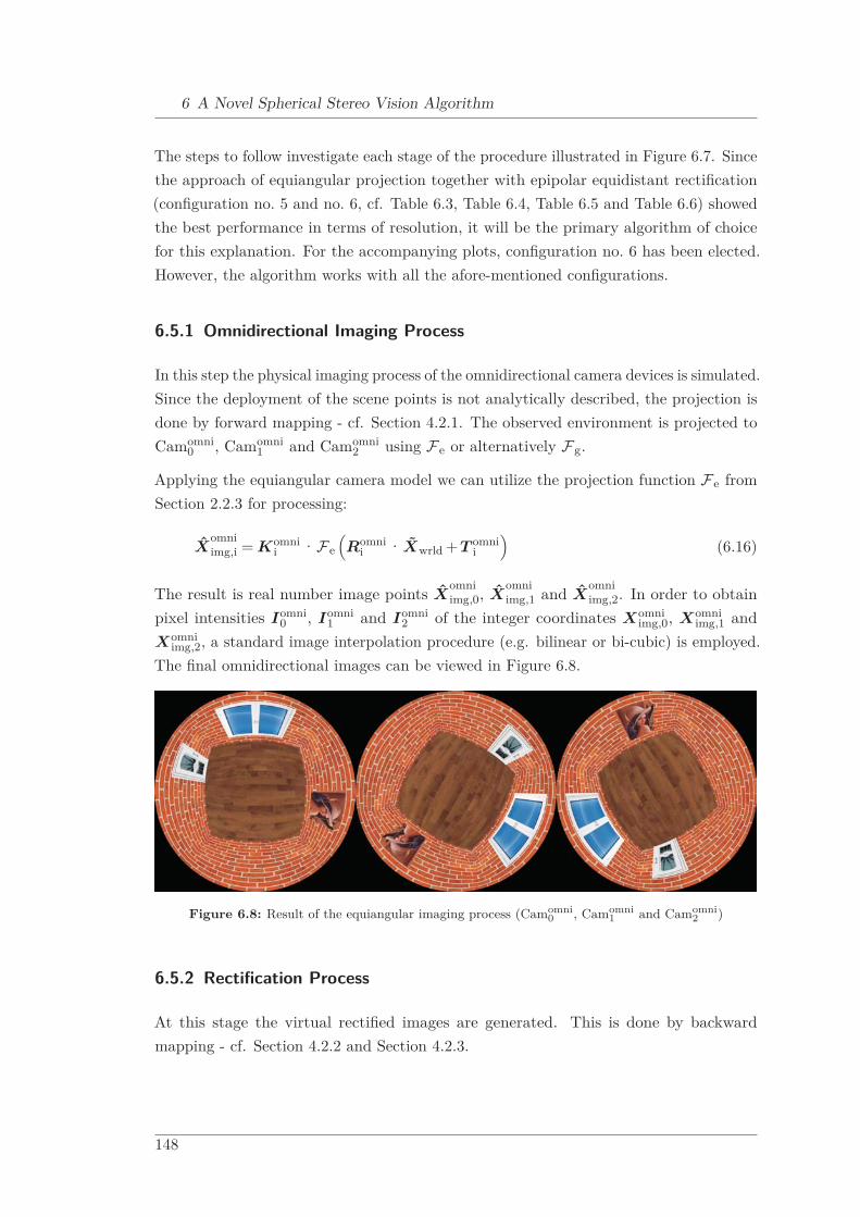
6 A Novel Spherical Stereo Vision Algorithm
The steps to follow investigate each stage of the procedure illustrated in Figure 6.7. Sincethe approach of equiangular projection together with epipolar equidistant rectification(configuration no. 5 and no. 6, cf. Table 6.3, Table 6.4, Table 6.5 and Table 6.6) showedthe best performance in terms of resolution, it will be the primary algorithm of choicefor this explanation. For the accompanying plots, configuration no. 6 has been elected.However, the algorithm works with all the afore-mentioned configurations.
6.5.1 Omnidirectional Imaging Process
In this step the physical imaging process of the omnidirectional camera devices is simulated.Since the deployment of the scene points is not analytically described, the projection isdone by forward mapping - cf. Section 4.2.1. The observed environment is projected toCamomni
0 , Camomni1 and Camomni
2 using Fe or alternatively Fg.
Applying the equiangular camera model we can utilize the projection function Fe fromSection 2.2.3 for processing:
Xomniimg,i = Komni
i ·Fe(Romni
i ·Xwrld +T omnii
)(6.16)
The result is real number image points Xomniimg,0, X
omniimg,1 and X
omniimg,2. In order to obtain
pixel intensities Iomni0 , Iomni
1 and Iomni2 of the integer coordinates Xomni
img,0, Xomniimg,1 and
Xomniimg,2, a standard image interpolation procedure (e.g. bilinear or bi-cubic) is employed.
The final omnidirectional images can be viewed in Figure 6.8.
Figure 6.8: Result of the equiangular imaging process (Camomni0 , Camomni
1 and Camomni2 )
6.5.2 Rectification Process
At this stage the virtual rectified images are generated. This is done by backwardmapping - cf. Section 4.2.2 and Section 4.2.3.
148

6.5 Spherical Depth Map Generation
Equivalently to Section 4.2.2, the target image mesh of pixel positions Xrectimg,j is set up
and back-projected to its appropriate world points Xrectwrld,j with respect to its dedicated
omnidirectional camera using F rect,1 (or alternatively F rect,2) inversely:
Xrectcam,j (λ) = λ·Rrect
j ·F−1rect,1
(Krect
j−1 ·Xrect
img,j
)(6.17)
In accordance to Section 4.2.2, the arbitrary scale factor λ expresses the one dimensionalspace of points on the ray. To overcome the uncertainty of distance from the cameracenter, we define
∥∥∥Xrectwrld,j
∥∥∥2
= 1.
In the following, those points are projected to their attached omnidirectional camera.Applying the equiangular camera model we can utilize the projection function Fe:
Xomniimg,0a = Komni
0 ·Fe(Romni
0 ·Xrectcam,0a
)X
omniimg,0b = Komni
0 ·Fe(Romni
0 ·Xrectcam,0b
)X
omniimg,1a = Komni
1 ·Fe(Romni
1 ·Xrectcam,1a
)X
omniimg,1c = Komni
1 ·Fe(Romni
1 ·Xrectcam,1c
)X
omniimg,2b = Komni
2 ·Fe(Romni
2 ·Xrectcam,2b
)X
omniimg,2c = Komni
2 ·Fe(Romni
2 ·Xrectcam,2c
)(6.18)
The result is real-numbered image points Xomniimg,j. In order to obtain pixel intensities Irect
j ,a standard image interpolation procedure (e.g. bilinear or bicubic) is used. The finalrectified images can be seen in Figure 6.9.
Figure 6.9: Result of the epipolar equidistant imaging process (Camrect0a , Camrect
1a , Camrect2b , Camrect
0b ,Camrect
1c , Camrect2c )
It can be seen that either of the two images are rectified with respect to each otherand therefore, since they have different positions Crect
j , form rectified stereo vision pairsSCamrect
k . This shows the effect described in Section 5.3.
149
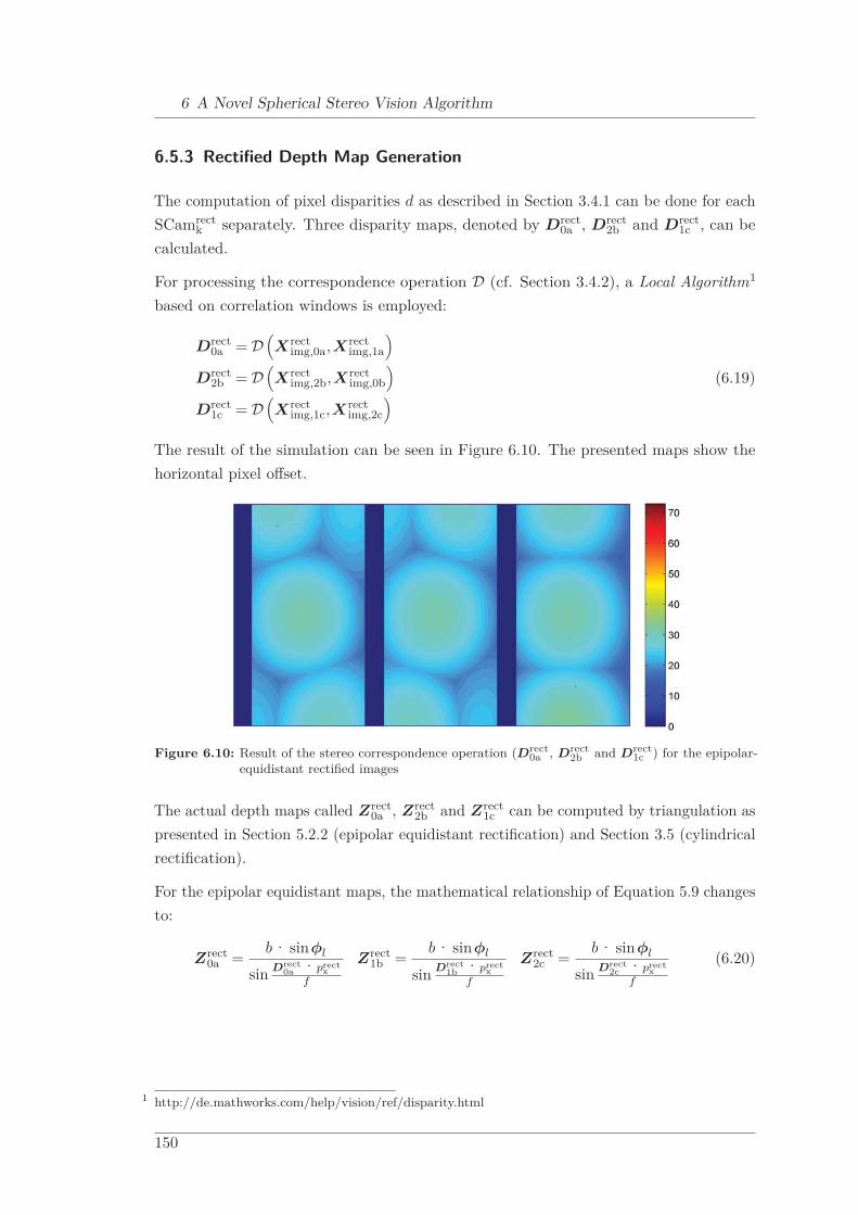
6 A Novel Spherical Stereo Vision Algorithm
6.5.3 Rectified Depth Map Generation
The computation of pixel disparities d as described in Section 3.4.1 can be done for eachSCamrect
k separately. Three disparity maps, denoted by Drect0a , Drect
2b and Drect1c , can be
calculated.
For processing the correspondence operation D (cf. Section 3.4.2), a Local Algorithm1
based on correlation windows is employed:
Drect0a = D
(Xrect
img,0a,Xrectimg,1a
)Drect
2b = D(Xrect
img,2b,Xrectimg,0b
)Drect
1c = D(Xrect
img,1c,Xrectimg,2c
) (6.19)
The result of the simulation can be seen in Figure 6.10. The presented maps show thehorizontal pixel offset.
Figure 6.10: Result of the stereo correspondence operation (Drect0a , Drect
2b and Drect1c ) for the epipolar-
equidistant rectified images
The actual depth maps called Zrect0a , Zrect
2b and Zrect1c can be computed by triangulation as
presented in Section 5.2.2 (epipolar equidistant rectification) and Section 3.5 (cylindricalrectification).
For the epipolar equidistant maps, the mathematical relationship of Equation 5.9 changesto:
Zrect0a =
b· sinφl
sin Drect0a ·prect
xf
Zrect1b =
b· sinφl
sin Drect1b ·prect
xf
Zrect2c =
b· sinφl
sin Drect2c ·prect
xf
(6.20)
1 http://de.mathworks.com/help/vision/ref/disparity.html
150
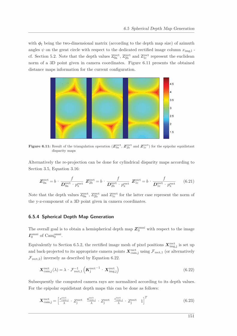
6.5 Spherical Depth Map Generation
with φl being the two-dimensional matrix (according to the depth map size) of azimuthangles ψ on the great circle with respect to the dedicated rectified image column ximg,l -cf. Section 5.2. Note that the depth values Zrect
0a , Zrect2b and Zrect
1c represent the euclideannorm of a 3D point given in camera coordinates. Figure 6.11 presents the obtaineddistance maps information for the current configuration.
Figure 6.11: Result of the triangulation operation (Zrect0a , Zrect
2b and Zrect1c ) for the epipolar equidistant
disparity maps
Alternatively the re-projection can be done for cylindrical disparity maps according toSection 3.5, Equation 3.16:
Zrect0a = b·
f
Drect0a ·prect
xZrect
2b = b·f
Drect2b ·prect
xZrect
1c = b·f
Drect1c ·prect
x(6.21)
Note that the depth values Zrect0a , Zrect
2b and Zrect1c for the latter case represent the norm of
the y-z-component of a 3D point given in camera coordinates.
6.5.4 Spherical Depth Map Generation
The overall goal is to obtain a hemispherical depth map Zomni0 with respect to the image
Iomni0 of Camomni
0 .
Equivalently to Section 6.5.2, the rectified image mesh of pixel positions Xrectimg,j is set up
and back-projected to its appropriate camera points Xrectcam,j using F rect,1 (or alternatively
F rect,2) inversely as described by Equation 6.22.
Xrectcam,j (λ) = λ·F−1
rect,1
(Krect
j−1 ·Xrect
img,j
)(6.22)
Subsequently the computed camera rays are normalized according to its depth values.For the epipolar equidistant depth maps this can be done as follows:
Xrectcam,j =
[xrect
cam,jλ ·Zrect
jyrect
cam,jλ ·Zrect
jzrect
cam,jλ ·Zrect
j 1]T
(6.23)
151
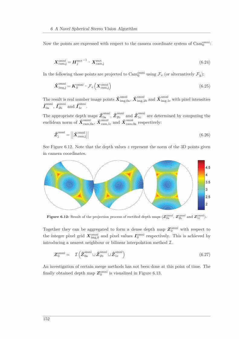
6 A Novel Spherical Stereo Vision Algorithm
Now the points are expressed with respect to the camera coordinate system of Camomni0 :
Xomnicam,j = Hrect
j−1 ·Xrect
cam,j (6.24)
In the following those points are projected to Camomni0 using Fe (or alternatively Fg):
Xomniimg,j = Komni
0 ·Fe(Xomni
cam,j
)(6.25)
The result is real number image points Xomniimg,0a, X
omniimg,2b and X
omniimg,1c with pixel intensities
Iomni0a , I
omni2b and I
omni1c .
The appropriate depth maps Zomni0a , Z
omni2b and Z
omni1c are determined by computing the
euclidean norm of Xomnicam,0a, X
omnicam,1c and X
omnicam,0a respectively:
Zomnij =
∣∣∣∣∣∣Xomnicam,j
∣∣∣∣∣∣ (6.26)
See Figure 6.12. Note that the depth values z represent the norm of the 3D points givenin camera coordinates.
Figure 6.12: Result of the projection process of rectified depth maps (Zomni0a , Zomni
2b and Zomni1c ).
Together they can be aggregated to form a dense depth map Zomni0 with respect to
the integer pixel grid Xomniimg,0 and pixel values Iomni
0 respectively. This is achieved byintroducing a nearest neighbour or bilinear interpolation method I.
Zomni0 = I
(Z
omni0a ∪ Z
omni2b ∪ Z
omni1c
)(6.27)
An investigation of certain merge methods has not been done at this point of time. Thefinally obtained depth map Zomni
0 is visualized in Figure 6.13.
152

6.5 Spherical Depth Map Generation
Figure 6.13: Merged depth map Zomni0
6.5.5 3D Reprojection
In order to check the calculated spherical depth map, the result shall be validated bya 3D reprojection. The integer spherical image grid Xomni
img,0 is reprojected employingEquation 2.15 and Equation 2.28 inversely:
Xomnicam,0 (λ) = λ·F−1
e
(Komni
0−1 ·Xomni
img,0
)(6.28)
The computed camera rays are subsequently scaled according to its depth values:
Xomnicam,0 =
[xomni
cam,0λ ·Zomni
0yomni
cam,0λ ·Zomni
0zomni
cam,0λ ·Zomni
0 1]T
(6.29)
Since Camomni0 represents the reference camera, its coordinate system coincides with the
world frame. That means the computed camera points Xomnicam,0 form the estimate Xwrld
of the original world points Xwrld:
Xomnicam,0=Xwrld (6.30)
The illustration in Figure 6.14 depicts the pixel values Iomni0 of the reference camera at
its estimated world positions Xwrld.
153

6 A Novel Spherical Stereo Vision Algorithm
Figure 6.14: 3D re-projection of the omnidirectional depth map Zomni0
6.6 Error Analysis
The accuracy and error effects that appear when stereo vision is processed have beendiscussed in Section 3.5 for an ordinary perspective two-view configuration. Accuracypreservation for virtual camera generation has been discussed in Section 4.4. At thispoint the expectable measurement errors for the presented stereo vision configurationshall be numerically evaluated and discussed.
In Chapter 3 it has been discussed that 3D measurement devices which rely on stereo visionface a considerable amount of error sources. Primarily these are inaccurate intrinsicallyand extrinsically calibrated setups or defective stereo correspondence results as a matterof principle. However in this section the focus is on imperfect depth measurements dueto a limited accuracy of the underlying pixel information and errors that are introduceddue to the special characteristics of the present system.
Although the configuration works in principle with each and every afore-discussedconfiguration (cf. Table 6.3, Table 6.4, Table 6.5 and Table 6.6) I will restrict thisinvestigation to epipolar equidistant rectification. It has shown the best achievableresolution.
154
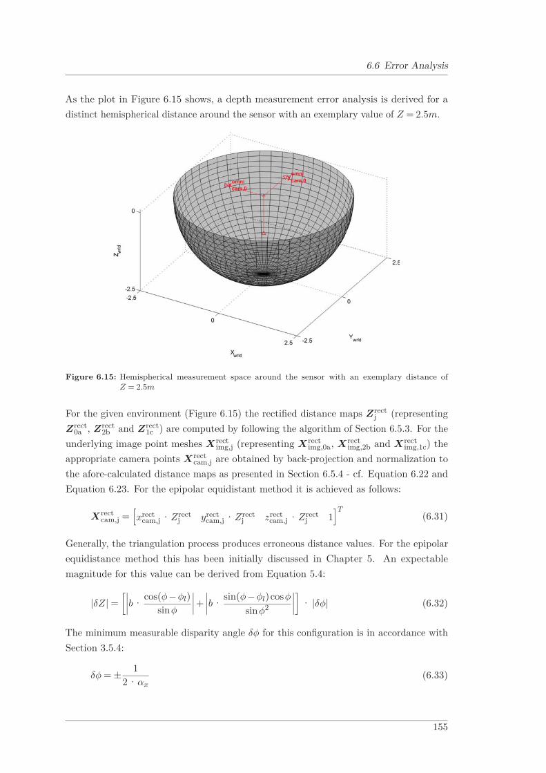
6.6 Error Analysis
As the plot in Figure 6.15 shows, a depth measurement error analysis is derived for adistinct hemispherical distance around the sensor with an exemplary value of Z = 2.5m.
Figure 6.15: Hemispherical measurement space around the sensor with an exemplary distance ofZ = 2.5m
For the given environment (Figure 6.15) the rectified distance maps Zrectj (representing
Zrect0a , Zrect
2b and Zrect1c ) are computed by following the algorithm of Section 6.5.3. For the
underlying image point meshes Xrectimg,j (representing Xrect
img,0a, Xrectimg,2b and Xrect
img,1c) theappropriate camera points Xrect
cam,j are obtained by back-projection and normalization tothe afore-calculated distance maps as presented in Section 6.5.4 - cf. Equation 6.22 andEquation 6.23. For the epipolar equidistant method it is achieved as follows:
Xrectcam,j =
[xrect
cam,j ·Zrectj yrect
cam,j ·Zrectj zrect
cam,j ·Zrectj 1
]T(6.31)
Generally, the triangulation process produces erroneous distance values. For the epipolarequidistance method this has been initially discussed in Chapter 5. An expectablemagnitude for this value can be derived from Equation 5.4:
|δZ| =[∣∣∣∣b·
cos(φ−φl)sinφ
∣∣∣∣+ ∣∣∣∣b·sin(φ−φl)cosφ
sinφ2
∣∣∣∣] · |δφ| (6.32)
The minimum measurable disparity angle δφ for this configuration is in accordance withSection 3.5.4:
δφ = ± 12·αx
(6.33)
155
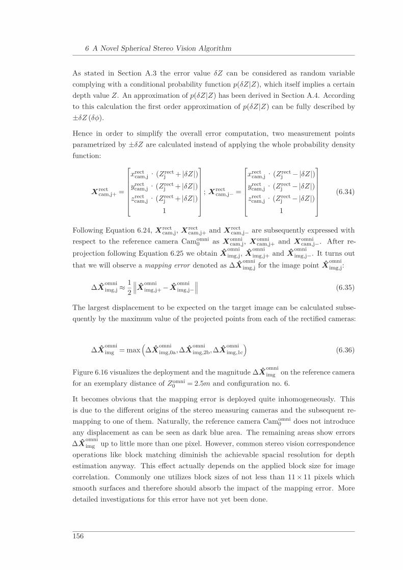
6 A Novel Spherical Stereo Vision Algorithm
As stated in Section A.3 the error value δZ can be considered as random variablecomplying with a conditional probability function p(δZ|Z), which itself implies a certaindepth value Z. An approximation of p(δZ|Z) has been derived in Section A.4. Accordingto this calculation the first order approximation of p(δZ|Z) can be fully described by±δZ (δφ).
Hence in order to simplify the overall error computation, two measurement pointsparametrized by ±δZ are calculated instead of applying the whole probability densityfunction:
Xrectcam,j+ =
⎡⎢⎢⎢⎢⎢⎢⎣xrect
cam,j ·(Zrectj + |δZ|)
yrectcam,j ·(Zrect
j + |δZ|)zrect
cam,j ·(Zrectj + |δZ|)1
⎤⎥⎥⎥⎥⎥⎥⎦ ; Xrectcam,j− =
⎡⎢⎢⎢⎢⎢⎢⎣xrect
cam,j ·(Zrectj −|δZ|)
yrectcam,j ·(Zrect
j −|δZ|)zrect
cam,j ·(Zrectj −|δZ|)1
⎤⎥⎥⎥⎥⎥⎥⎦ (6.34)
Following Equation 6.24, Xrectcam,j, Xrect
cam,j+ and Xrectcam,j− are subsequently expressed with
respect to the reference camera Camomni0 as Xomni
cam,j, Xomnicam,j+ and Xomni
cam,j−. After re-projection following Equation 6.25 we obtain X
omniimg,j, X
omniimg,j+ and X
omniimg,j−. It turns out
that we will observe a mapping error denoted as ΔXomniimg,j for the image point X
omniimg,j:
ΔXomniimg,j ≈ 1
2
∥∥∥Xomniimg,j+ −X
omniimg,j−
∥∥∥ (6.35)
The largest displacement to be expected on the target image can be calculated subse-quently by the maximum value of the projected points from each of the rectified cameras:
ΔXomniimg = max
(ΔX
omniimg,0a,ΔX
omniimg,2b,ΔX
omniimg,1c
)(6.36)
Figure 6.16 visualizes the deployment and the magnitude ΔXomniimg on the reference camera
for an exemplary distance of Zomni0 = 2.5m and configuration no. 6.
It becomes obvious that the mapping error is deployed quite inhomogeneously. Thisis due to the different origins of the stereo measuring cameras and the subsequent re-mapping to one of them. Naturally, the reference camera Camomni
0 does not introduceany displacement as can be seen as dark blue area. The remaining areas show errorsΔX
omniimg up to little more than one pixel. However, common stereo vision correspondence
operations like block matching diminish the achievable spacial resolution for depthestimation anyway. This effect actually depends on the applied block size for imagecorrelation. Commonly one utilizes block sizes of not less than 11 × 11 pixels whichsmooth surfaces and therefore should absorb the impact of the mapping error. Moredetailed investigations for this error have not yet been done.
156

6.6 Error Analysis
Figure 6.16: Maximum mapping error ΔXomniimg for an exemplary distance of Zomni
0 = 2.5m, an equian-gular projection model for the source camera, an epipolar equidistant projection model forthe target camera, a FOVH = 83.20o and a baselength of b = 15cm
Actually ΔXomniimg = 1 represents a certain observation angle which is numerically small.
For configuration no. 6 it can be calculated as follows:
ΔXomniimg
αx=
1526
= 0.0019=0.1o (6.37)
Furthermore ΔXomniimg varies according to multiple parameters:
• Stereo vision configuration: The larger the baselength b is, the higher the expectedmaximum mapping error ΔX
omniimg becomes for a certain distance under observation
and for a distinct parametrized minimum measurable distance.
• Measurement distance: The mapping error decreases with increasing measurementdistance Z. At infinity the different locations of the three cameras will becomemeaningless and hence ΔX
omniimg approaches zero.
• Virtual camera configuration: Currently the virtual views are sampled accordingto the under-sampling strategy - cf. Chapter 4. In the center of each virtual imageits resolution coincides with the underlying omnidirectional image. In contrast, theouter areas highly under-sample the source image. This leads to the effect that
157

6 A Novel Spherical Stereo Vision Algorithm
the mapping error increases especially in the outer areas, when erroneous distanceinformation from the virtual views is mapped to the omnidirectional referencecamera. Hence, a change to over-sampling would reduce ΔX
omniimg considerably.
Figure 6.17 outlines the calculated maximum mapping error for different configurationsand distances Z.
Figure 6.17: Maximum mapping error ΔXomniimg for multiple measurement distances and camera config-
urations
The actual depth error∣∣∣δZomni
j
∣∣∣ for Xomniimg,j can hence be estimated by orthogonal projection
of Xomnicam,j+ and Xomni
cam,j− to Xomnicam,j and subsequently subtracting the magnitudes as follows:
∣∣∣δZomnij
∣∣∣ =1
2∥∥∥Xomni
cam,j
∥∥∥(Xomni
cam,jT ·Xomni
cam,j+ −Xomnicam,j
T ·Xomnicam,j−
)(6.38)
A maximum distance error∣∣δZomni
max∣∣ on the target image can be calculated subsequently:
∣∣∣δZomnimax
∣∣∣ = max(∣∣∣δZomni
0a
∣∣∣ , ∣∣∣δZomni2b
∣∣∣ , ∣∣∣δZomni1c
∣∣∣) (6.39)
Figure 6.18 visualizes the deployment and the magnitude∣∣δZomni
max∣∣ on the reference camera
for an exemplary distance of Z = 2.5m and configuration no. 6. While the left plot shows
158
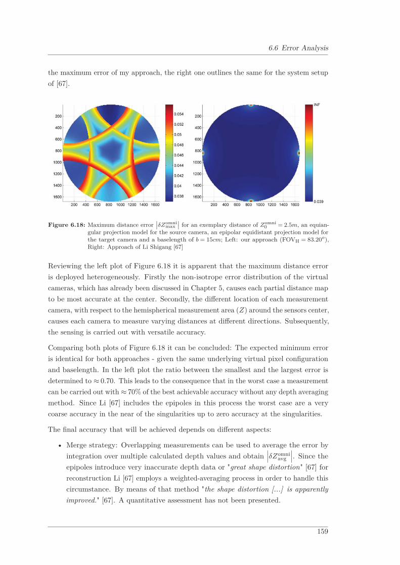
6.6 Error Analysis
the maximum error of my approach, the right one outlines the same for the system setupof [67].
Figure 6.18: Maximum distance error∣∣δZomni
max∣∣ for an exemplary distance of Zomni
0 = 2.5m, an equian-gular projection model for the source camera, an epipolar equidistant projection model forthe target camera and a baselength of b = 15cm; Left: our approach (FOVH = 83.20o),Right: Approach of Li Shigang [67]
Reviewing the left plot of Figure 6.18 it is apparent that the maximum distance erroris deployed heterogeneously. Firstly the non-isotrope error distribution of the virtualcameras, which has already been discussed in Chapter 5, causes each partial distance mapto be most accurate at the center. Secondly, the different location of each measurementcamera, with respect to the hemispherical measurement area (Z) around the sensors center,causes each camera to measure varying distances at different directions. Subsequently,the sensing is carried out with versatile accuracy.
Comparing both plots of Figure 6.18 it can be concluded: The expected minimum erroris identical for both approaches - given the same underlying virtual pixel configurationand baselength. In the left plot the ratio between the smallest and the largest error isdetermined to ≈ 0.70. This leads to the consequence that in the worst case a measurementcan be carried out with ≈ 70% of the best achievable accuracy without any depth averagingmethod. Since Li [67] includes the epipoles in this process the worst case are a verycoarse accuracy in the near of the singularities up to zero accuracy at the singularities.
The final accuracy that will be achieved depends on different aspects:
• Merge strategy: Overlapping measurements can be used to average the error byintegration over multiple calculated depth values and obtain
∣∣∣δZomniavg
∣∣∣. Since theepipoles introduce very inaccurate depth data or "great shape distortion" [67] forreconstruction Li [67] employs a weighted-averaging process in order to handle thiscircumstance. By means of that method "the shape distortion [...] is apparentlyimproved." [67]. A quantitative assessment has not been presented.
159
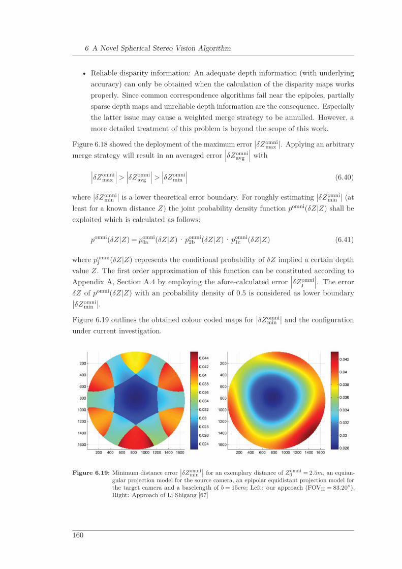
6 A Novel Spherical Stereo Vision Algorithm
• Reliable disparity information: An adequate depth information (with underlyingaccuracy) can only be obtained when the calculation of the disparity maps worksproperly. Since common correspondence algorithms fail near the epipoles, partiallysparse depth maps and unreliable depth information are the consequence. Especiallythe latter issue may cause a weighted merge strategy to be annulled. However, amore detailed treatment of this problem is beyond the scope of this work.
Figure 6.18 showed the deployment of the maximum error∣∣δZomni
max∣∣. Applying an arbitrary
merge strategy will result in an averaged error∣∣∣δZomni
avg
∣∣∣ with
∣∣∣δZomnimax
∣∣∣ >∣∣∣δZomni
avg
∣∣∣ >∣∣∣δZomni
min
∣∣∣ (6.40)
where∣∣δZomni
min∣∣ is a lower theoretical error boundary. For roughly estimating
∣∣δZomnimin
∣∣ (atleast for a known distance Z) the joint probability density function pomni(δZ|Z) shall beexploited which is calculated as follows:
pomni(δZ|Z) = pomni0a (δZ|Z)·pomni
2b (δZ|Z)·pomni1c (δZ|Z) (6.41)
where pomnij (δZ|Z) represents the conditional probability of δZ implied a certain depth
value Z. The first order approximation of this function can be constituted according toAppendix A, Section A.4 by employing the afore-calculated error
∣∣∣δZomnij
∣∣∣. The errorδZ of pomni(δZ|Z) with an probability density of 0.5 is considered as lower boundary∣∣δZomni
min∣∣.
Figure 6.19 outlines the obtained colour coded maps for∣∣δZomni
min∣∣ and the configuration
under current investigation.
Figure 6.19: Minimum distance error∣∣δZomni
min∣∣ for an exemplary distance of Zomni
0 = 2.5m, an equian-gular projection model for the source camera, an epipolar equidistant projection model forthe target camera and a baselength of b = 15cm; Left: our approach (FOVH = 83.20o),Right: Approach of Li Shigang [67]
160
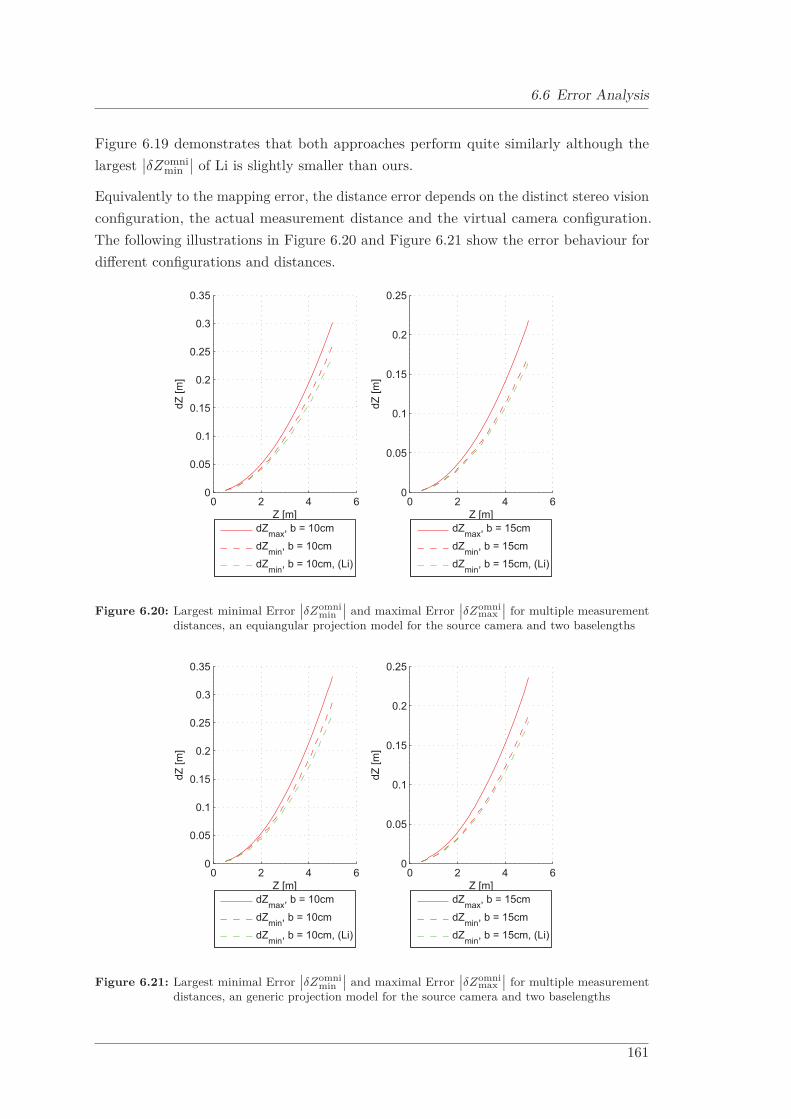
6.6 Error Analysis
Figure 6.19 demonstrates that both approaches perform quite similarly although thelargest
∣∣δZomnimin
∣∣ of Li is slightly smaller than ours.
Equivalently to the mapping error, the distance error depends on the distinct stereo visionconfiguration, the actual measurement distance and the virtual camera configuration.The following illustrations in Figure 6.20 and Figure 6.21 show the error behaviour fordifferent configurations and distances.
0 2 4 60
0.05
0.1
0.15
0.2
0.25
0.3
0.35
Z [m]
dZ [m
]
dZmax, b = 10cm
dZmin, b = 10cm
dZmin, b = 10cm, (Li)
0 2 4 60
0.05
0.1
0.15
0.2
0.25
Z [m]
dZ [m
]
dZmax, b = 15cm
dZmin, b = 15cm
dZmin, b = 15cm, (Li)
Figure 6.20: Largest minimal Error∣∣δZomni
min∣∣ and maximal Error
∣∣δZomnimax
∣∣ for multiple measurementdistances, an equiangular projection model for the source camera and two baselengths
0 2 4 60
0.05
0.1
0.15
0.2
0.25
0.3
0.35
Z [m]
dZ [m
]
dZmax, b = 10cm
dZmin, b = 10cm
dZmin, b = 10cm, (Li)
0 2 4 60
0.05
0.1
0.15
0.2
0.25
Z [m]
dZ [m
]
dZmax, b = 15cm
dZmin, b = 15cm
dZmin, b = 15cm, (Li)
Figure 6.21: Largest minimal Error∣∣δZomni
min∣∣ and maximal Error
∣∣δZomnimax
∣∣ for multiple measurementdistances, an generic projection model for the source camera and two baselengths
161
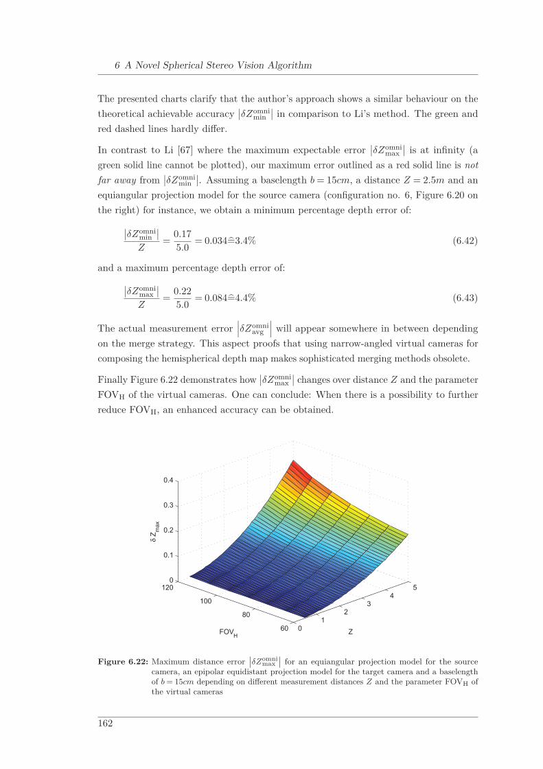
6 A Novel Spherical Stereo Vision Algorithm
The presented charts clarify that the author’s approach shows a similar behaviour on thetheoretical achievable accuracy
∣∣δZomnimin
∣∣ in comparison to Li’s method. The green andred dashed lines hardly differ.
In contrast to Li [67] where the maximum expectable error∣∣δZomni
max∣∣ is at infinity (a
green solid line cannot be plotted), our maximum error outlined as a red solid line is notfar away from
∣∣δZomnimin
∣∣. Assuming a baselength b = 15cm, a distance Z = 2.5m and anequiangular projection model for the source camera (configuration no. 6, Figure 6.20 onthe right) for instance, we obtain a minimum percentage depth error of:∣∣δZomni
min∣∣
Z=
0.175.0
= 0.034=3.4% (6.42)
and a maximum percentage depth error of:∣∣δZomnimax
∣∣Z
=0.225.0
= 0.084=4.4% (6.43)
The actual measurement error∣∣∣δZomni
avg
∣∣∣ will appear somewhere in between dependingon the merge strategy. This aspect proofs that using narrow-angled virtual cameras forcomposing the hemispherical depth map makes sophisticated merging methods obsolete.
Finally Figure 6.22 demonstrates how∣∣δZomni
max∣∣ changes over distance Z and the parameter
FOVH of the virtual cameras. One can conclude: When there is a possibility to furtherreduce FOVH, an enhanced accuracy can be obtained.
01
23
45
60
80
100
1200
0.1
0.2
0.3
0.4
ZFOVH
δ Z m
ax
Figure 6.22: Maximum distance error∣∣δZomni
max∣∣ for an equiangular projection model for the source
camera, an epipolar equidistant projection model for the target camera and a baselengthof b = 15cm depending on different measurement distances Z and the parameter FOVH ofthe virtual cameras
162
Chapter 7
Stereo Vision Demonstrator
This chapter treats a real system that shall demonstrate the practical feasibility of theafore-presented omnidirectional stereo method. In Section 7.1 the actual compiled cameraconfiguration is presented. Successively, the currently employed calibration strategy forthe system is explained in Section 7.2. In order to calculate a depth map, appropriaterectified views have to be configured. This is done in Section 7.3.
Finally, the C++ implementation that currently runs the system as well as first experi-mental results are outlined in Section 7.4 and Section 7.5.
7.1 Physical System Setup
The applied imaging system comprises three Allied GC940GC industry cameras (1-inchCMOSIS CMV4000 sensor with a full resolution of 2048×2048 pixels), each equippedwith a FE185C086HA-1 fisheye lens that is characterized by a focal length of f = 2.7mmand a field of view of 185◦. The captured images are cropped to an effective resolution of1680×1680 pixels.
The stereo vision setup, as can be seen in Figure 7.1, is specified in order to provide anapproximate baselength of b ≈ 10cm for each rectified stereo camera.
For capturing images the cameras have been triggered in order to record isochronously.The illustrations in Figure 7.2 show images that have been generated in the professorship’slab apartment.
163
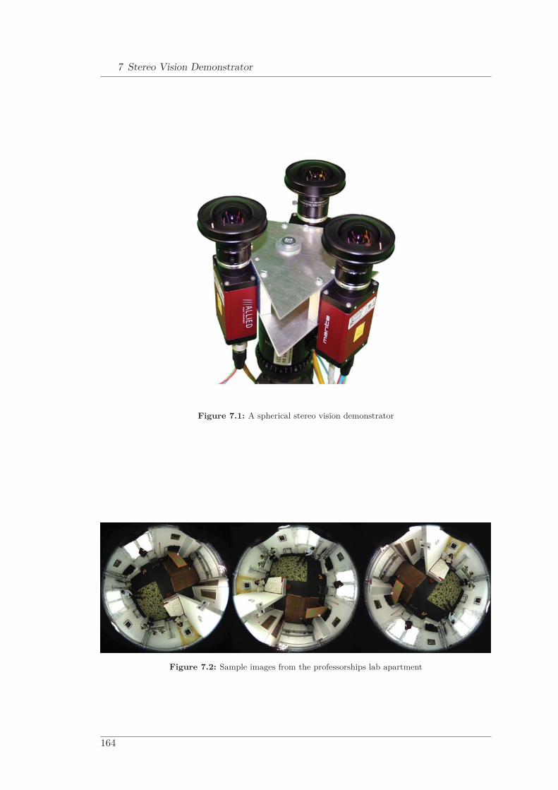
7 Stereo Vision Demonstrator
Figure 7.1: A spherical stereo vision demonstrator
Figure 7.2: Sample images from the professorships lab apartment
164
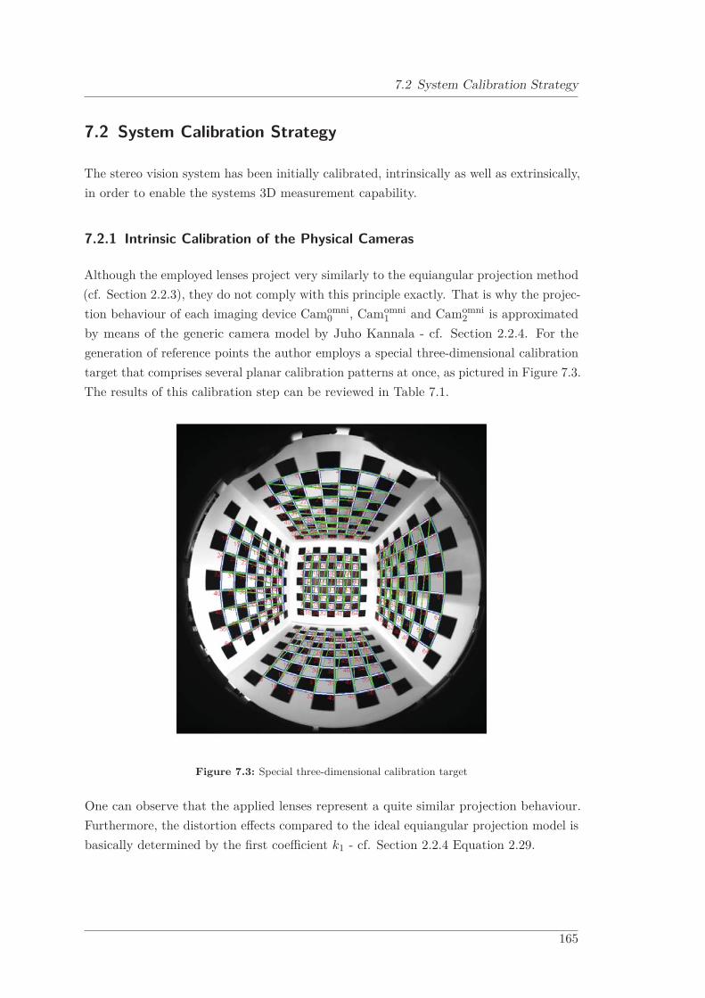
7.2 System Calibration Strategy
7.2 System Calibration Strategy
The stereo vision system has been initially calibrated, intrinsically as well as extrinsically,in order to enable the systems 3D measurement capability.
7.2.1 Intrinsic Calibration of the Physical Cameras
Although the employed lenses project very similarly to the equiangular projection method(cf. Section 2.2.3), they do not comply with this principle exactly. That is why the projec-tion behaviour of each imaging device Camomni
0 , Camomni1 and Camomni
2 is approximatedby means of the generic camera model by Juho Kannala - cf. Section 2.2.4. For thegeneration of reference points the author employs a special three-dimensional calibrationtarget that comprises several planar calibration patterns at once, as pictured in Figure 7.3.The results of this calibration step can be reviewed in Table 7.1.
Figure 7.3: Special three-dimensional calibration target
One can observe that the applied lenses represent a quite similar projection behaviour.Furthermore, the distortion effects compared to the ideal equiangular projection model isbasically determined by the first coefficient k1 - cf. Section 2.2.4 Equation 2.29.
165

7 Stereo Vision Demonstrator
Table 7.1: Results of the intrinsic generic camera models estimation
Camera k1 k2 αx αy cx cy k3 k4 k5
Camomni0 2.43 0.08 198.07 198.04 830.37 844.53 -0.04 0.03 -0.01
Camomni1 2.43 0.11 198.14 197.97 843.72 849.74 -0.11 0.07 -0.01
Camomni2 2.44 0.09 198.00 198.12 857.28 846.02 -0.07 0.04 -0.01
7.2.2 Extrinsic Calibration of the Physical and the Virtual Cameras
In Chapter 2 and Chapter 4 it is explained that the extrinsic parameters of eachphysical and virtual camera are fully described by the homography H (cf. Chapter 2Equation 2.20), comprising the cameras origin C and its rotation matrix R (composedof Euler Angles ϕx, ϕy and ϕz).
The applied calibration method utilizes two view geometry, as discussed in Section 2.4 -without optimization amongst all three views. Therefore, six virtual perspective cameras,denoted as Camper
j , are utilized. In combination, they compose three virtual perspectivestereo cameras, denoted as SCamper
k , for calibration. Their extrinsic parameters coincidewith those of Camrect
j , and SCamrectk respectively. This relationship is presented in
Equation 7.1. An adequate illustration, comparable with Figure 5.17 of Section 5.3, canbe reviewed in Figure 7.4.
SCampera = {Camper
0a ,Camper1a }
SCamperb = {Camper
2b ,Camper0b }
SCamperc = {Camper
1c ,Camper2c }
(7.1)
Figure 7.4: Geometrical configuration for extrinsic calibration of the physical and virtual cameras
166

7.2 System Calibration Strategy
7.2.2.1 Extrinsic Initialization of the Physical Cameras
Initially, it is assumed that each omnidirectional camera Camomnii is located at the worlds
origin Comnii = 0. Furthermore, two cameras are characterized by an ideal mutual rotation
of 23π around their own z-axes: ϕz
omni0 = 0, ϕz
omni1 = +2
3π and ϕzomni2 = −2
3π. This canbe justified by reviewing Figure 5.15 in Chapter 5. Thereby, initial extrinsic parametersare determined, denoted as Hiomni
0 , Hiomni1 and Hiomni
2 .
7.2.2.2 Extrinsic Initialization of the Virtual Cameras
At the beginning the virtual cameras inherit the extrinsic configuration from the omnidi-rectional cameras. To roughly pre-rectify each virtual stereo camera pair SCamper
k , eachleft camera (Camper
0a , Camper2b , Camper
1c ) of each pair is rotated around its z-axis towardsthe associate right camera (Camper
1a , Camper0b , Camper
2c ) by an angle of 13π, and vice versa.
In combination with the initial extrinsic parameters, determined in Section 7.2.2.1, theinitial homographies Hiper
j for the virtual perspective cameras can be calculated asfollows:
Hiper0a = dHiper
+ ·Hiomni0
Hiper0b = dHiper
− ·Hiomni0
Hiper1a = dHiper
− ·Hiomni1
Hiper1c = dHiper
+ ·Hiomni1
Hiper2b = dHiper
+ ·Hiomni2
Hiper2c = dHiper
− ·Hiomni2
(7.2)
where dHiper+ and dHiper
− determine the homographies describing a differential rotationaround the z-axis in positive direction, and negative direction respectively. Hence Hiper
j ,comprising Riper
j and Ciperj , represent the initial extrinsic estimates of the virtual
perspective cameras which roughly complies with the mechanical system configuration.
7.2.2.3 Two-View Stereo Calibration and Rectification
The subsequent calibration procedure is accomplished for each stereo camera SCamperk
independently. For instance, Figure 7.5 shows sample images that have been generatedfor calibrating stereo camera SCamper
a .
This process is performed in accordance with the description in Section 3.2. Therefore,the calibration toolbox by Bouguet [11] is applied for each stereo pair in order to obtaincalibration extrinsic estimates, denoted as Hc
per1a , Hc
per0b and Hc
per2c , for each of the right
167

7 Stereo Vision Demonstrator
Figure 7.5: Example calibration images for SCampera with original images from Camomni
0 (Hiomni0 )
and Camomni1 (Hiomni
1 ) as well as pre-rectified images from Camper0a (Hiper
0a ) and Camper1a
(Hiper1a )
cameras (Camper1a , Camper
0b and Camper2c ) with respect to their associate left ones (Camper
0a ,Camper
2b and Camper1c ).
The utilization of a rectification procedure for the calibrated images, as explained inSection 3.2 and described by Fusiello [28], results in new corrected homographies, denotedas Hr
pera , Hr
perb and Hr
perc , for each left and right perspective camera:
Hcper1a −→ Hr
pera
Hcper0b −→ Hr
perb
Hcper2c −→ Hr
perc
(7.3)
7.2.2.4 Three-View Stereo Rectification
The results of Section 7.2.2.3 are now used to locate the omnidirectional cameras Camomnii
extrinsically, as described by Equation 7.4. Three two-view calibrations for three concate-nated stereo cameras form an overdetermined configuration. By now, no optimizationmethod has been performed. Hence, the determination of the extrinsic parameters forthe fisheye cameras, denoted as Hc
omni0 , Hc
omni1 and Hc
omni2 , is performed on the basis
168
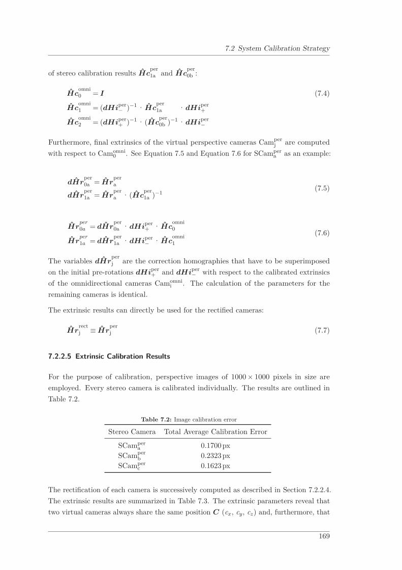
7.2 System Calibration Strategy
of stereo calibration results Hcper1a and Hc
per0b :
Hcomni0 = I (7.4)
Hcomni1 = (dHiper
− )−1 ·Hcper1a ·dHiper
+
Hcomni2 = (dHiper
+ )−1 ·(Hcper0b )−1 ·dHiper
−
Furthermore, final extrinsics of the virtual perspective cameras Camperj are computed
with respect to Camomni0 . See Equation 7.5 and Equation 7.6 for SCamper
a as an example:
dHrper0a = Hr
pera
dHrper1a = Hr
pera ·(Hc
per1a )−1
(7.5)
Hrper0a = dHr
per0a ·dHiper
+ ·Hcomni0
Hrper1a = dHr
per1a ·dHiper
− ·Hcomni1
(7.6)
The variables dHrperj are the correction homographies that have to be superimposed
on the initial pre-rotations dHiper+ and dHiper
− with respect to the calibrated extrinsicsof the omnidirectional cameras Camomni
i . The calculation of the parameters for theremaining cameras is identical.
The extrinsic results can directly be used for the rectified cameras:
Hrrectj ≡ Hr
perj (7.7)
7.2.2.5 Extrinsic Calibration Results
For the purpose of calibration, perspective images of 1000 × 1000 pixels in size areemployed. Every stereo camera is calibrated individually. The results are outlined inTable 7.2.
Table 7.2: Image calibration error
Stereo Camera Total Average Calibration Error
SCampera 0.1700px
SCamperb 0.2323px
SCamperc 0.1623px
The rectification of each camera is successively computed as described in Section 7.2.2.4.The extrinsic results are summarized in Table 7.3. The extrinsic parameters reveal thattwo virtual cameras always share the same position C (cx, cy, cz) and, furthermore, that
169

7 Stereo Vision Demonstrator
Table 7.3: Rectification results
Camera cx[mm] cy[mm] cz[mm] ϕx[rad] ϕy[rad] ϕz[rad]
Camper0a 0.00 0.00 0.00 0.0100 -0.0060 1.0573
Camper1a 48.00 -88.82 -0.61 0.0100 -0.0060 1.0573
Camper2b -52.90 -84.87 -0.20 -0.0023 0.0020 -1.0135
Camper0b 0.00 0.00 0.00 -0.0023 0.0020 -1.0135
Camper1c 48.00 -88.82 -0.61 0.0042 0.0020 -3.1058
Camper2c -52.90 -84.87 -0.20 0.0046 0.0015 -3.1038
three pairs of cameras coincide in terms of orientation R (ϕx, ϕy, ϕz), as a consequence ofrectification. However, this does not completely hold true for the stereo camera SCamper
c ,since the rotation parameters of the involved views slightly differ. This issue is indicatedby red color in Table 7.3.
However, Table 7.3 provides no information about the error in localizing Camomni1 and
Camomni2 with respect to Camomni
0 . In order to get an indication about that issue, acycle homography, denoted as Herr, is computed by incorporating all the calibrationinformation calculated. Initially, the actual cycle starts at Camomni
0 computing thehomography to Camomni
1 , based on this it computes the homography to Camomni2 and
finally it closes the circle by computing the homography back to Camomni0 . If the
calibration process had provided perfect results, the calculation as seen in Equation 7.8should have led to the identity matrix.
Herr = (dHiper− )−1 ·Hc
per0b ·dHiper
+︸ ︷︷ ︸Homography from Camomni
2 to Camomni0
· (dHiper− )−1 ·Hc
per2c ·dHiper
+︸ ︷︷ ︸Homography from Camomni
1 to Camomni2
· (dHiper− )−1 ·Hc
per1a ·dHiper
+︸ ︷︷ ︸Homography from Camomni
0 to Camomni1
Herr =
⎡⎣Rerr T err
0 1
⎤⎦(7.8)
The evaluation of this equation by employing the afore-computed numerical values leadsto Rerr ≈ I and |T err| > 5mm. This reveals that the utilized method, for calibrationof three cameras, is quite accurate in terms of rotation but not very satisfactory withrespect to translation. While one can now assume good results from the stereo matchingstage, the triangulation and the merge process of the depth maps leads us to expectperceptible errors.
170

7.3 Virtual Camera Setup
7.3 Virtual Camera Setup
Since the results of the intrinsic generic camera model estimation stage (Table 7.1) arequite similar to the generic parameters used for simulation (Table 4.2) and distinctrequirements are not claimed, configuration no. 7 is chosen for initial practical tests.The calculated parameters can be reviewed in Table 7.4 to Table 7.7. In contrast toconfiguration no. 7, the parameters for the vertical resolution are determined according tothe over-sampling strategy. This does not have any influence on the accuracy but causesthe final merged map to be more dense as can bee seen in Section 7.5. The variationsapplied have been marked with blue color in the tables.
Table 7.4: Calculated fields of view FOVh for the virtual cameras Camrectj according to the variety of
configurations
No. Camomnii Camrect
j b [m] FOVhr [deg] Zmin [m] FOVh [deg]
7 kannala9 epipolar equidistance 0.10 60.0 0.75 75.40
As can be seen in Table 7.5, indicated by red color, the parameter dmax for the maximumdisparity has been slightly adapted in order to comply with available procedures forstereo correspondence computation. Since for the stereo matching process the standardalgorithm from OpenCV StereoBM 1 is employed, which claims dmax to be a power oftwo, it has been changed from 65 to 64.
Table 7.5: Calculated virtual pixel size ratios and image sizes
No. FOVh [deg] prectx /pomni
x precty /pomni
y height width dmax
7 75.40 0.4140 0.4577 1680 636 64
Table 7.6: Intrinsic parameters of the virtual cameras Camrectj
No. Camera αx αy cx cy
7 Camrectj 483.71 534.76 318.50 839.5
Table 7.7: Pixel dimensions of the virtual cameras Camrectj
No. Camera px[m] py[m]
7 Camrectj 5.58×10⁻⁶ 5.05×10⁻⁶
1 http://docs.opencv.org/modules/calib3d/doc/camera_calibration_and_3d_reconstruction.html
171
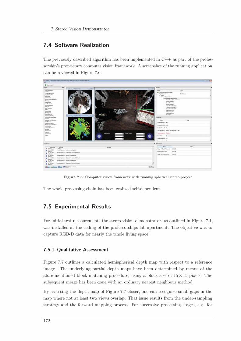
7 Stereo Vision Demonstrator
7.4 Software Realization
The previously described algorithm has been implemented in C++ as part of the profes-sorship’s proprietary computer vision framework. A screenshot of the running applicationcan be reviewed in Figure 7.6.
Figure 7.6: Computer vision framework with running spherical stereo project
The whole processing chain has been realized self-dependent.
7.5 Experimental Results
For initial test measurements the stereo vision demonstrator, as outlined in Figure 7.1,was installed at the ceiling of the professorships lab apartment. The objective was tocapture RGB-D data for nearly the whole living space.
7.5.1 Qualitative Assessment
Figure 7.7 outlines a calculated hemispherical depth map with respect to a referenceimage. The underlying partial depth maps have been determined by means of theafore-mentioned block matching procedure, using a block size of 15 × 15 pixels. Thesubsequent merge has been done with an ordinary nearest neighbour method.
By assessing the depth map of Figure 7.7 closer, one can recognize small gaps in themap where not at least two views overlap. That issue results from the under-samplingstrategy and the forward mapping process. For successive processing stages, e.g. for
172
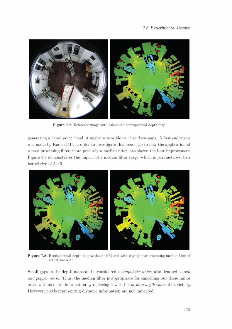
7.5 Experimental Results
Figure 7.7: Reference image with calculated hemispherical depth map
generating a dense point cloud, it might be sensible to close these gaps. A first endeavourwas made by Kaden [51], in order to investigate this issue. Up to now the application ofa post processing filter, more precisely a median filter, has shown the best improvement.Figure 7.8 demonstrates the impact of a median filter stage, which is parametrized to akernel size of 5×5.
Figure 7.8: Hemispherical depth map without (left) and with (right) post processing median filter ofkernel size 5 × 5
Small gaps in the depth map can be considered as impulsive noise, also denoted as saltand pepper noise. Thus, the median filter is appropriate for cancelling out these minorareas with no depth information by replacing it with the median depth value of its vicinity.However, pixels representing distance information are not impacted.
173
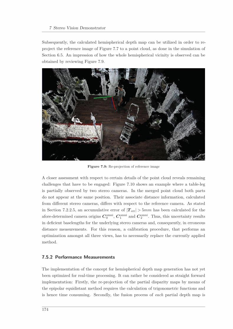
7 Stereo Vision Demonstrator
Subsequently, the calculated hemispherical depth map can be utilized in order to re-project the reference image of Figure 7.7 to a point cloud, as done in the simulation ofSection 6.5. An impression of how the whole hemispherical vicinity is observed can beobtained by reviewing Figure 7.9.
Figure 7.9: Re-projection of reference image
A closer assessment with respect to certain details of the point cloud reveals remainingchallenges that have to be engaged: Figure 7.10 shows an example where a table-legis partially observed by two stereo cameras. In the merged point cloud both partsdo not appear at the same position. Their associate distance information, calculatedfrom different stereo cameras, differs with respect to the reference camera. As statedin Section 7.2.2.5, an accumulative error of |T err| > 5mm has been calculated for theafore-determined camera origins Comni
0 , Comni1 and Comni
2 . Thus, this uncertainty resultsin deficient baselengths for the underlying stereo cameras and, consequently, in erroneousdistance measurements. For this reason, a calibration procedure, that performs anoptimization amongst all three views, has to necessarily replace the currently appliedmethod.
7.5.2 Performance Measurements
The implementation of the concept for hemispherical depth map generation has not yetbeen optimized for real-time processing. It can rather be considered as straight forwardimplementation: Firstly, the re-projection of the partial disparity maps by means ofthe epipolar equidistant method requires the calculation of trigonometric functions andis hence time consuming. Secondly, the fusion process of each partial depth map is
174

7.5 Experimental Results
Figure 7.10: Example case for an erroneous fusion result
done by a forward mapping process. Further non-optimized parts include the nearestneighbour interpolation stage as well as the post processing filter. Besides the needfor improvement with respect to practical implementations, Chapter 8 will introduceoptimization strategies that will accelerate the current algorithm significantly. Initialperformance measurements have been realized on an Intel(R) Core (TM) i7-3520M CPU@ 2.90 GHz and are presented in Table 7.8. The actual timing values have been roundedsensibly. The obtained speed in terms of Frames Per Second (FPS) can be considered asnear real-time.
Table 7.8: Performance measurements
Ster
eoB
lock
size
Dep
thm
apm
erge
Pos
tP
roce
ssin
g
Ster
eoco
mpu
tati
on[m
s]
Re-
proj
ecti
on[m
s]
Dep
thm
apm
erge
[ms]
Pos
tfil
ter
[ms]
Tot
alfp
s
11×11 nearest neighbour no post processing 750 100 480 0 0.75
15×15 nearest neighbour no post processing 780 100 470 0 0.74
21×21 nearest neighbour no post processing 800 100 450 0 0.74
11×11 nearest neighbour median filter 5×5 750 100 480 150 0.67
15×15 nearest neighbour median filter 5×5 780 100 470 130 0.67
21×21 nearest neighbour median filter 5×5 800 100 450 120 0.68
175


Chapter 8
Discussion and Outlook
The so far achieved results with respect to the novel concept for spherical stereo vision arerevisited in this final chapter. A discussion of the achievements is presented in Section 8.1.Based on this assessment, further need for research is derived.
Furthermore, the idea of omnidirectional stereo vision, as investigated in this thesis,is compared to the approach by Li [67], and moreover, to a solution employing twohemispherical views in Section 8.2.
The end of this thesis is constituted by the presentation of a demo application that utilizesspherical depth data in Section 8.3, and last but not least, by summarizing remarks inSection 8.4.
8.1 Discussion of the Current Results and Further Need forResearch
The major objective of this thesis was to investigate a new principle in order generate afull hemispherical depth map by means of stereo vision. Based on known methods, asoutlined in Chapter 5, an alternative approach to Li [67] has been presented that shallfulfil the following requirements:
1. A full hemispherical depth map shall be generated without the need of applying amerging procedure of high computational effort.
2. The proposed approach shall generate a full hemispherical depth map by employingfewer correspondence operations.
In the following, the investigations that have been performed in order to achieve theafore-mentioned goals shall be reflected and assessed. In addition, proposals for furtherresearch activities and for algorithm optimization are presented.
177
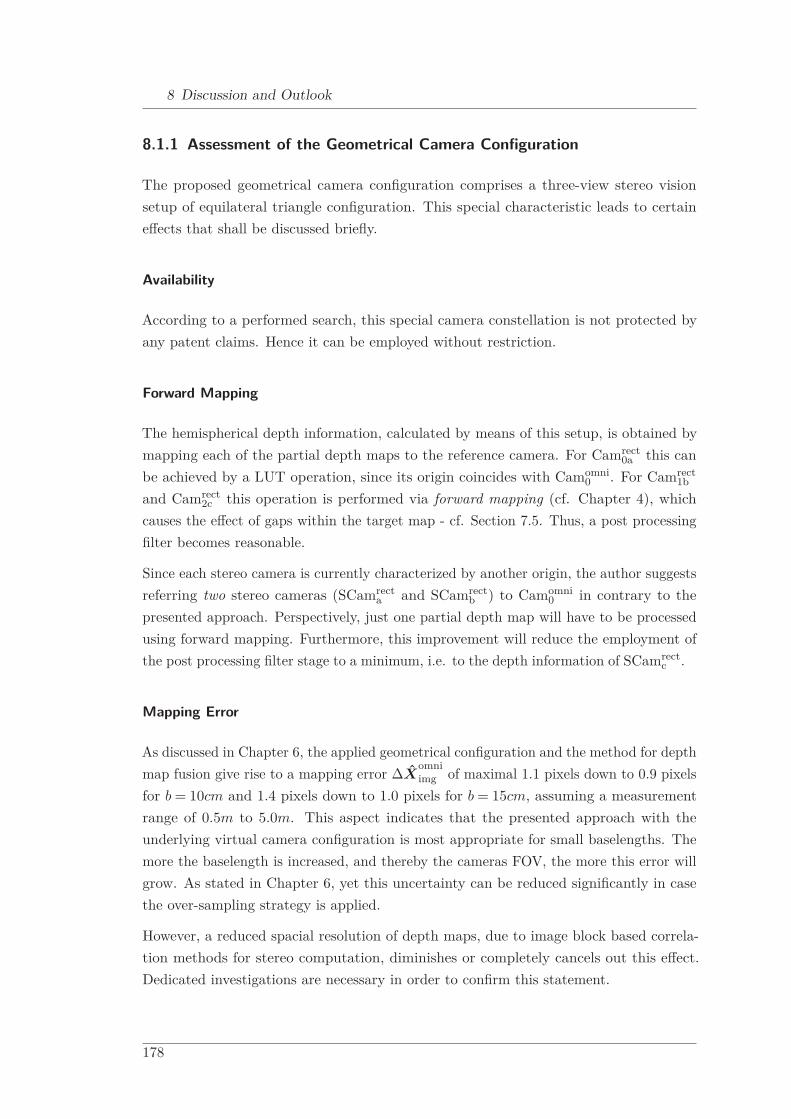
8 Discussion and Outlook
8.1.1 Assessment of the Geometrical Camera Configuration
The proposed geometrical camera configuration comprises a three-view stereo visionsetup of equilateral triangle configuration. This special characteristic leads to certaineffects that shall be discussed briefly.
Availability
According to a performed search, this special camera constellation is not protected byany patent claims. Hence it can be employed without restriction.
Forward Mapping
The hemispherical depth information, calculated by means of this setup, is obtained bymapping each of the partial depth maps to the reference camera. For Camrect
0a this canbe achieved by a LUT operation, since its origin coincides with Camomni
0 . For Camrect1b
and Camrect2c this operation is performed via forward mapping (cf. Chapter 4), which
causes the effect of gaps within the target map - cf. Section 7.5. Thus, a post processingfilter becomes reasonable.
Since each stereo camera is currently characterized by another origin, the author suggestsreferring two stereo cameras (SCamrect
a and SCamrectb ) to Camomni
0 in contrary to thepresented approach. Perspectively, just one partial depth map will have to be processedusing forward mapping. Furthermore, this improvement will reduce the employment ofthe post processing filter stage to a minimum, i.e. to the depth information of SCamrect
c .
Mapping Error
As discussed in Chapter 6, the applied geometrical configuration and the method for depthmap fusion give rise to a mapping error ΔX
omniimg of maximal 1.1 pixels down to 0.9 pixels
for b = 10cm and 1.4 pixels down to 1.0 pixels for b = 15cm, assuming a measurementrange of 0.5m to 5.0m. This aspect indicates that the presented approach with theunderlying virtual camera configuration is most appropriate for small baselengths. Themore the baselength is increased, and thereby the cameras FOV, the more this error willgrow. As stated in Chapter 6, yet this uncertainty can be reduced significantly in casethe over-sampling strategy is applied.
However, a reduced spacial resolution of depth maps, due to image block based correla-tion methods for stereo computation, diminishes or completely cancels out this effect.Dedicated investigations are necessary in order to confirm this statement.
178
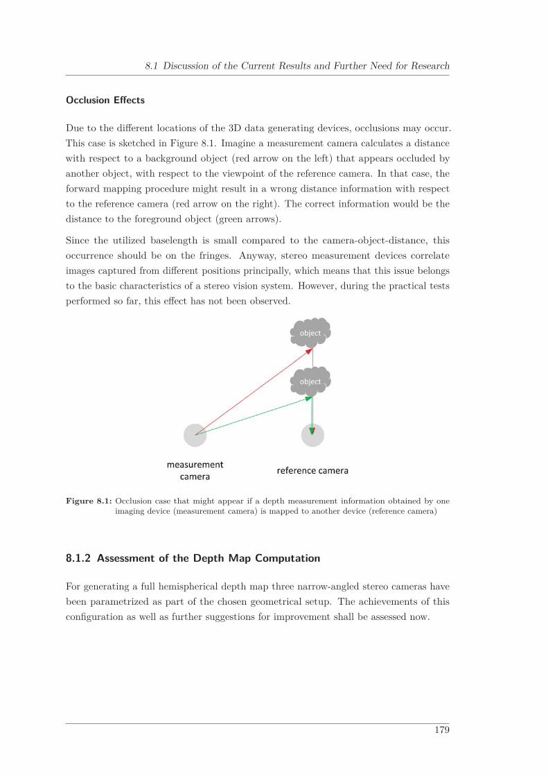
8.1 Discussion of the Current Results and Further Need for Research
Occlusion Effects
Due to the different locations of the 3D data generating devices, occlusions may occur.This case is sketched in Figure 8.1. Imagine a measurement camera calculates a distancewith respect to a background object (red arrow on the left) that appears occluded byanother object, with respect to the viewpoint of the reference camera. In that case, theforward mapping procedure might result in a wrong distance information with respectto the reference camera (red arrow on the right). The correct information would be thedistance to the foreground object (green arrows).
Since the utilized baselength is small compared to the camera-object-distance, thisoccurrence should be on the fringes. Anyway, stereo measurement devices correlateimages captured from different positions principally, which means that this issue belongsto the basic characteristics of a stereo vision system. However, during the practical testsperformed so far, this effect has not been observed.
Figure 8.1: Occlusion case that might appear if a depth measurement information obtained by oneimaging device (measurement camera) is mapped to another device (reference camera)
8.1.2 Assessment of the Depth Map Computation
For generating a full hemispherical depth map three narrow-angled stereo cameras havebeen parametrized as part of the chosen geometrical setup. The achievements of thisconfiguration as well as further suggestions for improvement shall be assessed now.
179

8 Discussion and Outlook
Parametrization of the Narrow-Angled Views
The presumption was that each view ought to cover a horizontal field of view of 60o
approximately - cf. Chapter 5 Section 5.3.1. Appropriate investigations in Chapter 6identified the necessity of a larger FOV for each rectified image, since the maximumdisparity value for guaranteeing a minimum measurable distance had to be included intothe calculations. The actual values for the current configuration have been determined to75.80o (b = 10cm) and 83.20o (b = 15cm) provided an epipolar equidistance rectificationmodel. The cylindrical projection method has been declined since it turned out togenerate target images of lower resolution and hence less accuracy compared to thealternative method. However, Abraham et al. [3] describe this projection principle tobe beneficial for stereo matching performance. Thus it could be beneficial to perform acompetitive evaluation for rectification methods with respect to their stereo matchingperformance in future.
Considering a real-time implementation, the usability of a rectification method that doesnot employ any trigonometric functions should be investigated. Thereby, the performancefor the triangulation process could be accelerated. As an example the stereographicrectification method has been briefly introduced in Section 5.2.
Stereo Correspondence Reduction
For an estimation of the currently achieved savings in terms of stereo correspondenceoperations the author assumes that Li [67] chooses the same sampling rate as presentedin Chapter 6. As mentioned in Chapter 5 he correlates two full images, while theauthor performs this operation on three partial images. Table 8.1 outlines the currentachievements.
Table 8.1: Savings in terms of stereo correspondence operations
No. Camomnii b [m] Zmin [m] FOVh [deg] height width savings [%]
5 equiangular 0.10 0.75 75.40 1344 699 30.06 equiangular 0.15 0.75 83.20 1285 763 23.07 kannala9 0.10 0.75 75.40 1254 636 37.28 kannala9 0.15 0.75 83.20 1201 702 30.6
It is important to realize that the achievements of Table 8.1 highly depend on theparametrization, above all, of the baselength and of the minimum allowable measurementdistance.
180
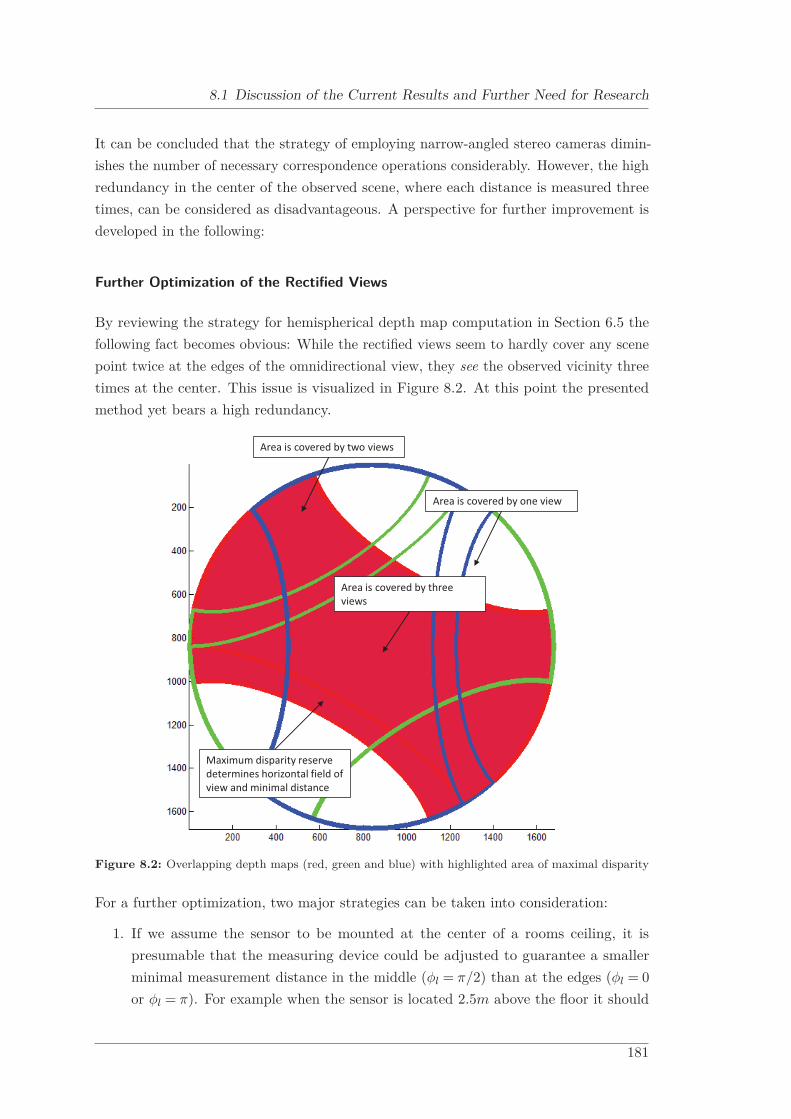
8.1 Discussion of the Current Results and Further Need for Research
It can be concluded that the strategy of employing narrow-angled stereo cameras dimin-ishes the number of necessary correspondence operations considerably. However, the highredundancy in the center of the observed scene, where each distance is measured threetimes, can be considered as disadvantageous. A perspective for further improvement isdeveloped in the following:
Further Optimization of the Rectified Views
By reviewing the strategy for hemispherical depth map computation in Section 6.5 thefollowing fact becomes obvious: While the rectified views seem to hardly cover any scenepoint twice at the edges of the omnidirectional view, they see the observed vicinity threetimes at the center. This issue is visualized in Figure 8.2. At this point the presentedmethod yet bears a high redundancy.
Area is covered by two views
Area is covered by three views
Area is covered by one view
Maximum disparity reserve determines horizontal field of view and minimal distance
Figure 8.2: Overlapping depth maps (red, green and blue) with highlighted area of maximal disparity
For a further optimization, two major strategies can be taken into consideration:
1. If we assume the sensor to be mounted at the center of a rooms ceiling, it ispresumable that the measuring device could be adjusted to guarantee a smallerminimal measurement distance in the middle (φl = π/2) than at the edges (φl = 0or φl = π). For example when the sensor is located 2.5m above the floor it should
181

8 Discussion and Outlook
allow a minimal distance of 0.5m in order to recognize a person that stands beneathand is 2m in height. At the edges the minimal distance could be parametrizedto 0.75m for example. The basic idea is to enlarge the disparity reserve in themiddle and decrease it at the edges. By that the presented concept could also workproperly in environments with reduced ceiling heights.
2. Since realistic requirements naturally demand the algorithm to process as fast aspossible, it makes sense to optimize the stereo processing itself with respect to thepartial rectified views: At the top of the rectified images (first image row) as wellas the bottom (last image row), the originally parametrized FOV for 3D calculationshould be preserved which means that the whole image line is considered by thestereo correspondence algorithm. When approaching the center row of the imagefrom either direction, the FOV for stereo processing could be reduced. By meansof that, an almost non-recurring coverage of each scene point could be achieved.Hence, the computational load for stereo processing as well as the forward mappingprocedure would further decrease considerably.
8.1.3 Assessment of the Depth Measurement Error
By employing narrow-angled views for stereo processing the variance of determined depthmeasurement uncertainties, within the same partial depth map, is constrained at closerange. The example of Chapter 6, Figure 6.18 plotted the error values
∣∣δZomnimax
∣∣ for theoverlapping partial depth maps of configuration no. 6 measuring a distance of 2.5m. Theminimum error to be observed has been determined to ≈ 3.8cm, and the maximum errorto ≈ 5.5cm respectively. The observed differential of ≈ 30% leads the author to theconclusion that a merge method of high computational effort as used by Li [67] has notto be implemented. Because of the small range of the error values, a simple averagingmethod is adequate. However, until now methods for merging depth maps have not beeninvestigated sufficiently.
Comparing the largest error value of∣∣δZomni
min∣∣ ≈ 4.3cm in the right plot of Chapter 6,
Figure 6.19 (approach Li [67]) with the largest error value∣∣δZomni
max∣∣ ≈ 5.5cm in the left
plot of Chapter 6, Figure 6.18 (authors approach), one can conclude the following:Without applying any depth averaging method, the presented approach obtains for theconfiguration in discussion at least approximately 80% of the accuracy achievable bycompetitors. The measurement errors can hence be considered as comparable. Thisstatement holds true if the following assumption is made: The significant accuracy of a3D sensor is specified by the worst case error value that occurs in its observation area(for a certain distance).
182
8.1 Discussion of the Current Results and Further Need for Research
8.1.4 Assessment of the Spherical Stereo Vision Demonstrator
As part of the thesis a demo setup has been assembled and presented in Chapter 7.The current status of this development and open points are briefly summarized in thefollowing:
Calibration Results
For the intrinsic calibration stage a state-of-the-art generic camera model has beenapplied. The utilized extrinsic calibration method (based on standard two-view geometry)turned out not to provide the required precision. While the mutual orientation of thecameras could be determined quite well, the translational offset between them led toa cumulative error of about 5mm. This gives rise to erroneous measurements due todeficiently determined baselengths, as could be seen in Chapter 7. Any MATLAB®
simulation the author performed, did not reveal inaccuracies of that kind. Hence, for anaccurate alignment of the partial point clouds, a more sophisticated calibration methodwill have to be applied in future necessarily. Advanced methods compute a trifocal tensorthat, equivalently to the fundamental matrix for two views, directly describe the inherentrelationship between three views. This issue represents a further field for research.
Results of the Depth Map Computation
As a result of Chapter 7, a full hemispherical depth map was presented, obtainedby realizing the author’s concept. The reprojection of this 3D data set generated aconsiderable point cloud. However, since the calibration process has yet to be optimizedfor accurate point cloud alignment, the validation of achieved measurements versuscomputed error values could not be carried out so far.
Computational Performance
As stated in Chapter 7 the current performance, which has been determined to slightlyless than 1FPS on a standard office PC hardware, can be considered as near real-time.Nevertheless, the current implementation has not yet been optimized, because the thesisfocuses on the principle investigation of the new method.
In comparison to Li [67], a real-time implementation of the author’s concept should befast due to the following facts:
• Currently the necessary stereo correspondence operations for obtaining a fullhemispherical depth map could be reduced to approximately 70%. A furtherreduction is possible as already stated.
183
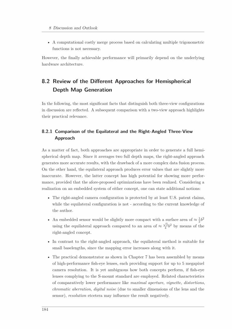
8 Discussion and Outlook
• A computational costly merge process based on calculating multiple trigonometricfunctions is not necessary.
However, the finally achievable performance will primarily depend on the underlyinghardware architecture.
8.2 Review of the Different Approaches for HemisphericalDepth Map Generation
In the following, the most significant facts that distinguish both three-view configurationsin discussion are reflected. A subsequent comparison with a two-view approach highlightstheir practical relevance.
8.2.1 Comparison of the Equilateral and the Right-Angled Three-ViewApproach
As a matter of fact, both approaches are appropriate in order to generate a full hemi-spherical depth map. Since it averages two full depth maps, the right-angled approachgenerates more accurate results, with the drawback of a more complex data fusion process.On the other hand, the equilateral approach produces error values that are slightly moreinaccurate. However, the latter concept has high potential for showing more perfor-mance, provided that the afore-proposed optimizations have been realized. Considering arealization on an embedded system of either concept, one can state additional notions:
• The right-angled camera configuration is protected by at least U.S. patent claims,while the equilateral configuration is not - according to the current knowledge ofthe author.
• An embedded sensor would be slightly more compact with a surface area of ≈ 12b2
using the equilateral approach compared to an area of ≈√
34 b2 by means of the
right-angled concept.
• In contrast to the right-angled approach, the equilateral method is suitable forsmall baselengths, since the mapping error increases along with it.
• The practical demonstrator as shown in Chapter 7 has been assembled by meansof high-performance fish-eye lenses, each providing support for up to 5 megapixelcamera resolution. It is yet ambiguous how both concepts perform, if fish-eyelenses complying to the S-mount standard are employed. Related characteristicsof comparatively lower performance like maximal aperture, vignette, distortions,chromatic aberration, digital noise (due to smaller dimensions of the lens and thesensor), resolution etcetera may influence the result negatively.
184
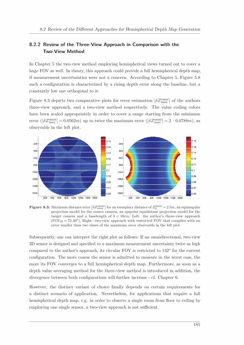
8.2 Review of the Different Approaches for Hemispherical Depth Map Generation
8.2.2 Review of the Three-View Approach in Comparison with theTwo-View Method
In Chapter 5 the two-view method employing hemispherical views turned out to cover ahuge FOV as well. In theory, this approach could provide a full hemispherical depth map,if measurement uncertainties were not a concern. According to Chapter 5, Figure 5.8such a configuration is characterized by a rising depth error along the baseline, but aconstantly low one orthogonal to it.
Figure 8.3 depicts two comparative plots for error estimation∣∣δZomni
max∣∣ of the authors
three-view approach, and a two-view method respectively. The value coding colorshave been scaled appropriately in order to cover a range starting from the minimumerror (
∣∣δZomnimax
∣∣ = 0.0562m) up to twice the maximum error (∣∣δZomni
max∣∣ = 2·0.0788m), as
observable in the left plot.
Figure 8.3: Maximum distance error∣∣δZomni
max∣∣ for an exemplary distance of Zomni
0 = 2.5m, an equiangularprojection model for the source camera, an epipolar equidistant projection model for thetarget camera and a baselength of b = 10cm; Left: the author’s three-view approach(FOVH = 75.40o), Right: two-view approach with restricted FOV that complies with anerror smaller than two times of the maximum error observable in the left plot
Subsequently, one can interpret the right plot as follows: If an omnidirectional, two-view3D sensor is designed and specified to a maximum measurement uncertainty twice as highcompared to the author’s approach, its circular FOV is restricted to 132o for the currentconfiguration. The more coarse the sensor is admitted to measure in the worst case, themore its FOV converges to a full hemispherical depth map. Furthermore, as soon as adepth value averaging method for the three-view method is introduced in addition, thedivergence between both configurations will further increase - cf. Chapter 6.
However, the distinct variant of choice finally depends on certain requirements fora distinct scenario of application. Nevertheless, for applications that require a fullhemispherical depth map, e.g. in order to observe a single room from floor to ceiling byemploying one single sensor, a two-view approach is not sufficient.
185
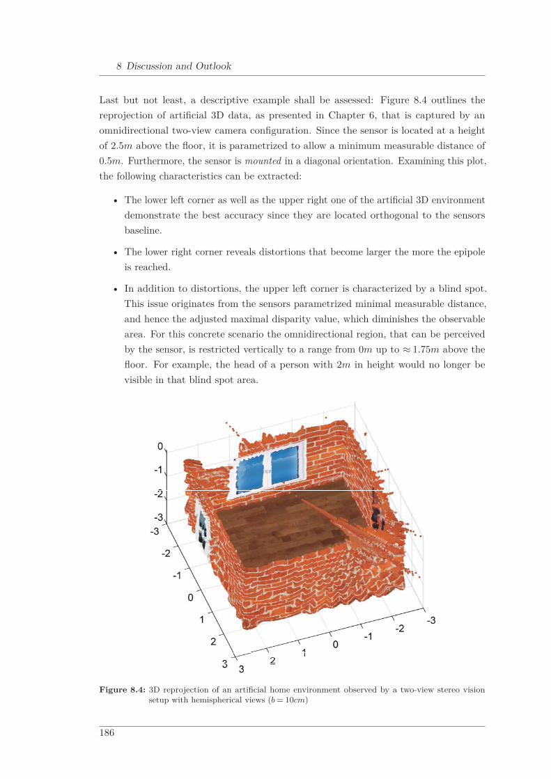
8 Discussion and Outlook
Last but not least, a descriptive example shall be assessed: Figure 8.4 outlines thereprojection of artificial 3D data, as presented in Chapter 6, that is captured by anomnidirectional two-view camera configuration. Since the sensor is located at a heightof 2.5m above the floor, it is parametrized to allow a minimum measurable distance of0.5m. Furthermore, the sensor is mounted in a diagonal orientation. Examining this plot,the following characteristics can be extracted:
• The lower left corner as well as the upper right one of the artificial 3D environmentdemonstrate the best accuracy since they are located orthogonal to the sensorsbaseline.
• The lower right corner reveals distortions that become larger the more the epipoleis reached.
• In addition to distortions, the upper left corner is characterized by a blind spot.This issue originates from the sensors parametrized minimal measurable distance,and hence the adjusted maximal disparity value, which diminishes the observablearea. For this concrete scenario the omnidirectional region, that can be perceivedby the sensor, is restricted vertically to a range from 0m up to ≈ 1.75m above thefloor. For example, the head of a person with 2m in height would no longer bevisible in that blind spot area.
Figure 8.4: 3D reprojection of an artificial home environment observed by a two-view stereo visionsetup with hemispherical views (b = 10cm)
186

8.3 A Sample Algorithm for Human Behaviour Analysis
8.3 A Sample Algorithm for Human Behaviour Analysis
For a convenient closure of this thesis, a detour to a practical application is made. InFigure 8.5 a system is depicted that applies an omnidirectional 3D sensor for humanbehaviour analysis. The algorithm as outlined has been published by the author in ascientific paper [26].
Omnidirectional Stereo Camera
RGB Data
Depth Data World-Z Map
Pose Estimation
Camera Calibration
Virtual PTZ
Behavior Analysis
Object Detection
People Hypothesis Generation
Figure 8.5: Structure of the proposed algorithm
In the following each single step is briefly explained.
Omnidirectional RGB-D Data Generation
The omnidirectional stereo camera provides hemispherical RGB-D data. Since the depthmeasuring device is extrinsically calibrated, with respect to a world coordinate system onthe floor of the observed scene, a world-z map can be calculated. Actually, this specifiesa map of distance values representing the height of each scene detail over ground.
People Hypothesis Generation
Position information about present persons in a room constitutes the precondition for asuccessive analysis of their behaviour. Robust person detection algorithms that employ3D data have recently been proposed [99]. In this study hypotheses about movingforeground objects, e.g. persons, are generated by applying a Gaussian Mixture Model(GMM) to the world-z map. In order to localize the potential persons with respect toworld coordinates, points belonging to these hypotheses are projected into a virtualoverhead view on which separate clusters are extracted. The detected persons are definedby the center, the orientation and the expansions of each cluster (Figure 8.6). Detailscan be reviewed in [99].
187
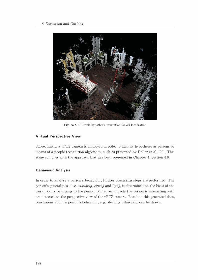
8 Discussion and Outlook
Figure 8.6: People hypothesis generation for 3D localization
Virtual Perspective View
Subsequently, a vPTZ camera is employed in order to identify hypotheses as persons bymeans of a people recognition algorithm, such as presented by Dollar et al. [20]. Thisstage complies with the approach that has been presented in Chapter 4, Section 4.6.
Behaviour Analysis
In order to analyse a person’s behaviour, further processing steps are performed. Theperson’s general pose, i. e. standing, sitting and lying, is determined on the basis of theworld points belonging to the person. Moreover, objects the person is interacting withare detected on the perspective view of the vPTZ camera. Based on this generated data,conclusions about a person’s behaviour, e. g. sleeping behaviour, can be drawn.
188

8.4 Closing Remarks
8.4 Closing Remarks
During the elaboration of this thesis, a couple of aspects related to spherical stereo visionhave been investigated. First of all, the primary objective of verifying the feasibility ofthe proposed concept could be achieved. A measurement system has been developed,which has great potential for future application fields in industry, security in public spacesas well as home environments. Furthermore, the amount of possible research topics,which has been generated in the course of this work, is considerable and thus providesa scientific prospect as well. Anyway, I hope the perusal of this thesis has been bothinformative and interesting to the reader.
189


Appendix A
Relevant Mathematics
This part outlines important mathematics and derivations.
A.1 Cross Product by Skew Symmetric Matrix
The cross product of two vectors a = (a1,a2,a3)T and b = (b1, b2, b3)T can be representedas dot product:
a×b = [a]×b =(aT [b]×
)T(A.1)
with
[a]× =
⎡⎢⎢⎢⎣0 −a3 a2
a3 0 −a1
−a2 a1 0
⎤⎥⎥⎥⎦ (A.2)
A.2 Derivation of the Quantization Error
A depth Z for stereo vision devices can be computed as follows:
Z = b·f
ad(A.3)
An depth measurement error can be specified as absolute depth error δZ:
δZ = δZb + δZf + δZd =f
dδb+
b
dδf − bf
d2 δd (A.4)
191
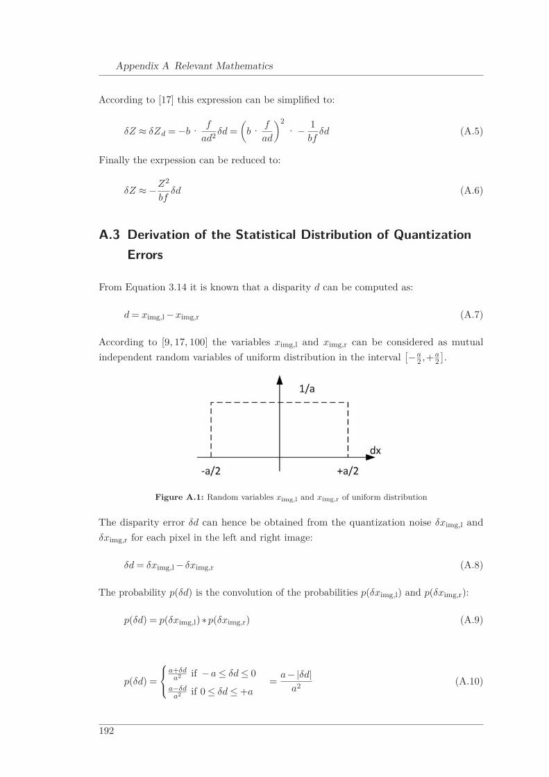
Appendix A Relevant Mathematics
According to [17] this expression can be simplified to:
δZ ≈ δZd = −b·f
ad2 δd =(
b·f
ad
)2· − 1
bfδd (A.5)
Finally the exrpession can be reduced to:
δZ ≈ −Z2
bfδd (A.6)
A.3 Derivation of the Statistical Distribution of QuantizationErrors
From Equation 3.14 it is known that a disparity d can be computed as:
d = ximg,l −ximg,r (A.7)
According to [9, 17, 100] the variables ximg,l and ximg,r can be considered as mutualindependent random variables of uniform distribution in the interval
[−a2 ,+a
2].
Figure A.1: Random variables ximg,l and ximg,r of uniform distribution
The disparity error δd can hence be obtained from the quantization noise δximg,l andδximg,r for each pixel in the left and right image:
δd = δximg,l − δximg,r (A.8)
The probability p(δd) is the convolution of the probabilities p(δximg,l) and p(δximg,r):
p(δd) = p(δximg,l)∗p(δximg,r) (A.9)
p(δd) =
⎧⎨⎩a+δd
a2 if −a ≤ δd ≤ 0a−δd
a2 if 0 ≤ δd ≤ +a=
a−|δd|a2 (A.10)
192

A.3 Derivation of the Statistical Distribution of Quantization Errors
The probability p(δZ) can be computed as follows:
p(δZ) =∫ +∞
−∞p(δZ|Z)p(Z)dZ (A.11)
where p(δZ|Z) is the conditional probability of δZ implied a certain depth value Z thatcan be measured with the probability p(Z).
It is known that the depth error δZ can be computed as:
δZ = −Z2
bf(δximg,l − δximg,r) = −Z2
bfδd (A.12)
which means that the disparity value δd is a monotone function of δZ:
δd = − bf
Z2 δZ = −a∗Z∗
Z2 δZ = −aZ∗
2Z2 δZ (A.13)
Since Equation A.13 is a monotone function, the probability p(δZ|Z) can be modelled asfollows:
p(δZ|Z) = p(δd)· | d(δd)d(δZ)
| =a−|δd|
a2 ·aZ∗
2Z2
=[1− |δd|
a
]·
Z∗
2Z2
(A.14)
Using Equation A.13 this expression can be simplified further:
p(δZ|Z) = p(δd)· | d(δd)d(δZ)
| =Z∗
2Z2 −(
Z∗
2Z2
)2|δZ| with 0 ≤ δZ ≤ Z∗
2Z2 (A.15)
Now Equation A.11 can be rewritten as follows:
p(δZ) =∫ +∞
−∞
[Z∗
2Z2 −(
Z∗
2Z2
)2|δZ|
]p(Z)dZ (A.16)
According to [17], the measured depth Z can only be randomly distributed over a limitedrange between Zmin and Zmax:
Zmin ≤ Z ≤ Zmax (A.17)
Furthermore from Equation A.15 it holds true that:
Z >=√
12
Z∗ · |δZ| (A.18)
For Equation A.16 it follows that:
p(δZ) =∫ Zmax
max(
Zmin,√
12 Z∗ · |δZ|
)[ Z∗
2Z2 −(
Z∗
2Z2
)2|δZ|
]p(Z)dZ (A.19)
193
Appendix A Relevant Mathematics
From Equation A.19 it can be concluded that the distribution of the depth error can beoutlined if a certain depth measurement distribution is known or assumed, e.g. uniformdistribution.
Since the disparity d can be assumed to be distributed uniformly in the interval [−a,+a]as mentioned above, the distribution of Z can be assumed to be distributed uniformly inthe interval [Zmin,Zmax]:
Zmin = Z − 12
Z2
bfδZ
Zmax = Z +12
Z2
bfδZ
(A.20)
Finally Equation A.19 can be solved for the intervals of Z separately.
When 0 ≤ |δZ| ≤ 2Zmin2
Z∗ it can be written:
p(δZ) =∫ Zmax
Zmin
[Z∗
2Z2 −(
Z∗
2Z2
)2|δZ|
]p(Z)dZ (A.21)
When 2Zmin2
Z∗ ≤ |δZ| ≤ 2Zmax2
Z∗ it can be written:
p(δZ) =∫ Zmax√
12 Z∗ · |δZ|
[Z∗
2Z2 −(
Z∗
2Z2
)2|δZ|
]p(Z)dZ (A.22)
Solving both integrals, the final probability distribution p(δZ) can be stated as follows:
p(δZ) =
⎧⎪⎨⎪⎩Z∗
2ZmaxZmin− (Z∗)2(Zmin2+ZminZmax+Zmax2)
12(ZminZmax)3 · |δZ| if 0 ≤ |δZ| ≤ 2Zmin2
Z∗
1Zmax−Zmin
[23
√Z∗
2|δZ| + (Z∗)2
12Zmax3 · |δZ|− Z∗2Zmax
]if 2Zmin2
Z∗ ≤ |δZ| ≤ 2Zmax2
Z∗
(A.23)
A.4 Approximation of the Quantization Error for EquiangularGeometry
A distance Z for fish-eye stereo devices can be calculated with respect to the left cameraas follows:
Z = b·sinφr
sin(φl −φr)= b·
sinφr
sin(φ)(A.24)
194

A.4 Approximation of the Quantization Error for Equiangular Geometry
A first order error δZ for a certain given Z (and hence φl as well as φ) can be estimatedby deviation:
δZ =[b·
cos(φ−φl)sinφ
−φ·sin(φ−φl)cosφ
sinφ2
]·δφ (A.25)
The disparity error δφ results for the statistical treatment from an error of the measuredangles φl in the left image and φr in the right image respectively:
δZ =[b·
cos(φ−φl)sinφ
−φ·sin(φ−φl)cosφ
sinφ2
]·
1αx
(δximg,l − δximg,r) (A.26)
As stated in Section A.3 the variables ximg,l and ximg,r can be considered as mutualindependent random variables of uniform distribution in the interval
[−a2 ,+a
2]
[17].
A probability density function p(δZ|Z) for a given Z can hence be approximated by:
p(δZ|Z) =[b·
cos(φ−φl)sinφ
−φ·sin(φ−φl)cosφ
sinφ2
]·
1αx︸ ︷︷ ︸
| d(δφ)d(δZ) |
·p(δφ) (A.27)
with
p(δφ) = p(δximg,l)∗p(δximg,r) (A.28)
Note that Equation A.27 represents a first order approximation of p(δZ|Z). If required,higher order approximations can be generated corresponding to the Taylor series ap-proximation. As an example the parametrization b = 1.0e−1m,f = 2.7e−3m,px =5.0e−6m,Z = 2.5m,φl = π/2 shall be employed. Figure A.2 outlines approximated nor-malized probability density functions pn of first and second order as well as a numericallyevaluated density function for comparison. The latter has been determined using aMATLAB® kernel smoothing density function1 estimation command following Bowmanet al. [14].
Furthermore a first order error value ±‖δZ‖ is outlined in Figure A.2 as black dashedlines based on the minimum measurable physical disparity angle δφ [17]:
δφ = ± 12·αx
(A.29)
It is recognizable that it coincides with a probability density value of exactly 0.5 for thefirst order approximation of the probability density function p(δZ|Z).
1 http://de.mathworks.com/help/stats/ksdensity.html
195

Appendix A Relevant Mathematics
−0.1 −0.05 0 0.05 0.10
0.1
0.2
0.3
0.4
0.5
0.6
0.7
0.8
0.9
1
δ Z
p n(δ Z
|Z)
Numerical evaluationFirst order approximationSecond order approximationδ Z based on disparity inacurracy
Figure A.2: Normalized probability density function
196
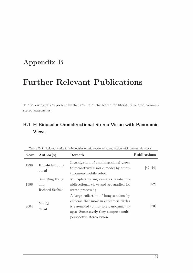
Appendix B
Further Relevant Publications
The following tables present further results of the search for literature related to omni-stereo approaches.
B.1 H-Binocular Omnidirectional Stereo Vision with PanoramicViews
Table B.1: Related works in h-binocular omnidirectional stereo vision with panoramic views
Year Author(s) Remark Publications
1990 Hiroshi Ishiguroet. al
Investigation of omnidirectional viewsto reconstruct a world model by an au-tonomous mobile robot.
[42–44]
1996Sing Bing KangandRichard Szeliski
Multiple rotating cameras create om-nidirectional views and are applied forstereo processing.
[52]
2004Yin Liet. al
A large collection of images taken bycameras that move in concentric circlesis assembled to multiple panoramic im-ages. Successively they compute multi-perspective stereo vision.
[70]
197
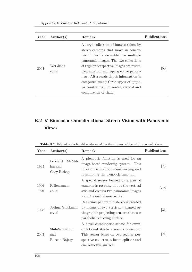
Appendix B Further Relevant Publications
Year Author(s) Remark Publications
2004Wei Jianget. al
A large collection of images taken bystereo cameras that move in concen-tric circles is assembled to multiplepanoramic images. The two collectionsof regular perspective images are resam-pled into four multi-perspective panora-mas. Afterwards depth information iscomputed using three types of epipo-lar constraints: horizontal, vertical andcombination of them.
[50]
B.2 V-Binocular Omnidirectional Stereo Vision with PanoramicViews
Table B.2: Related works in v-binocular omnidirectional stereo vision with panoramic views
Year Author(s) Remark Publications
1995Leonard McMil-lan andGary Bishop
A plenoptic function is used for animage-based rendering system. Thisrelies on sampling, reconstructing andre-sampling the plenoptic function.
[78]
19961998
R.Benosmanet. al
A special sensor formed by a pair ofcameras is rotating about the verticalaxis and creates two panoramic imagesfor 3D scene reconstruction.
[7, 8]
1998Joshua Gluckmanet. al
Real-time panoramic stereo is createdby means of two vertically aligned or-thographic projecting sensors that useparabolic reflecting surface.
[31]
2003Shih-Schon LinandRuzena Bajcsy
A novel catadioptric sensor for omni-directional stereo vision is presented.This sensor bases on two regular per-spective cameras, a beam splitter andone reflective surface.
[71]
198
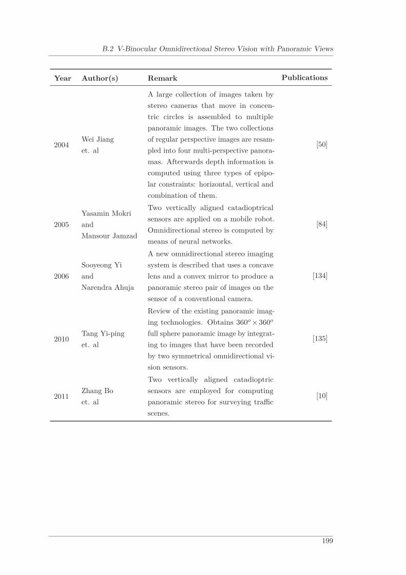
B.2 V-Binocular Omnidirectional Stereo Vision with Panoramic Views
Year Author(s) Remark Publications
2004Wei Jianget. al
A large collection of images taken bystereo cameras that move in concen-tric circles is assembled to multiplepanoramic images. The two collectionsof regular perspective images are resam-pled into four multi-perspective panora-mas. Afterwards depth information iscomputed using three types of epipo-lar constraints: horizontal, vertical andcombination of them.
[50]
2005Yasamin MokriandMansour Jamzad
Two vertically aligned catadioptricalsensors are applied on a mobile robot.Omnidirectional stereo is computed bymeans of neural networks.
[84]
2006Sooyeong YiandNarendra Ahuja
A new omnidirectional stereo imagingsystem is described that uses a concavelens and a convex mirror to produce apanoramic stereo pair of images on thesensor of a conventional camera.
[134]
2010Tang Yi-pinget. al
Review of the existing panoramic imag-ing technologies. Obtains 360o × 360o
full sphere panoramic image by integrat-ing to images that have been recordedby two symmetrical omnidirectional vi-sion sensors.
[135]
2011Zhang Boet. al
Two vertically aligned catadioptricsensors are employed for computingpanoramic stereo for surveying trafficscenes.
[10]
199
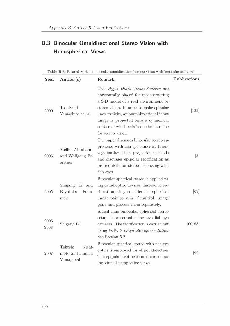
Appendix B Further Relevant Publications
B.3 Binocular Omnidirectional Stereo Vision withHemispherical Views
Table B.3: Related works in binocular omnidirectional stereo vision with hemispherical views
Year Author(s) Remark Publications
2000ToshiyukiYamashita et. al
Two Hyper-Omni-Vision-Sensors arehorizontally placed for reconstructinga 3-D model of a real environment bystereo vision. In order to make epipolarlines straight, an ominidirectional inputimage is projected onto a cylindricalsurface of which axis is on the base linefor stereo vision.
[133]
2005Steffen Abrahamand Wolfgang Fo-erstner
The paper discusses binocular stereo ap-proaches with fish-eye cameras. It sur-veys mathematical projection methodsand discusses epipolar rectification aspre-requisite for stereo processing withfish-eyes.
[3]
2005Shigang Li andKiyotaka Fuku-mori
Binocular spherical stereo is applied us-ing catadioptric devices. Instead of rec-tification, they consider the sphericalimage pair as sum of multiple imagepairs and process them separately.
[69]
20062008
Shigang Li
A real-time binocular spherical stereosetup is presented using two fish-eyecameras. The rectification is carried outusing latitude-longitude representation.See Section 5.2.
[66, 68]
2007Takeshi Nishi-moto and JunichiYamaguchi
Binocular spherical stereo with fish-eyeoptics is employed for object detection.The epipolar rectification is carried us-ing virtual perspective views.
[92]
200
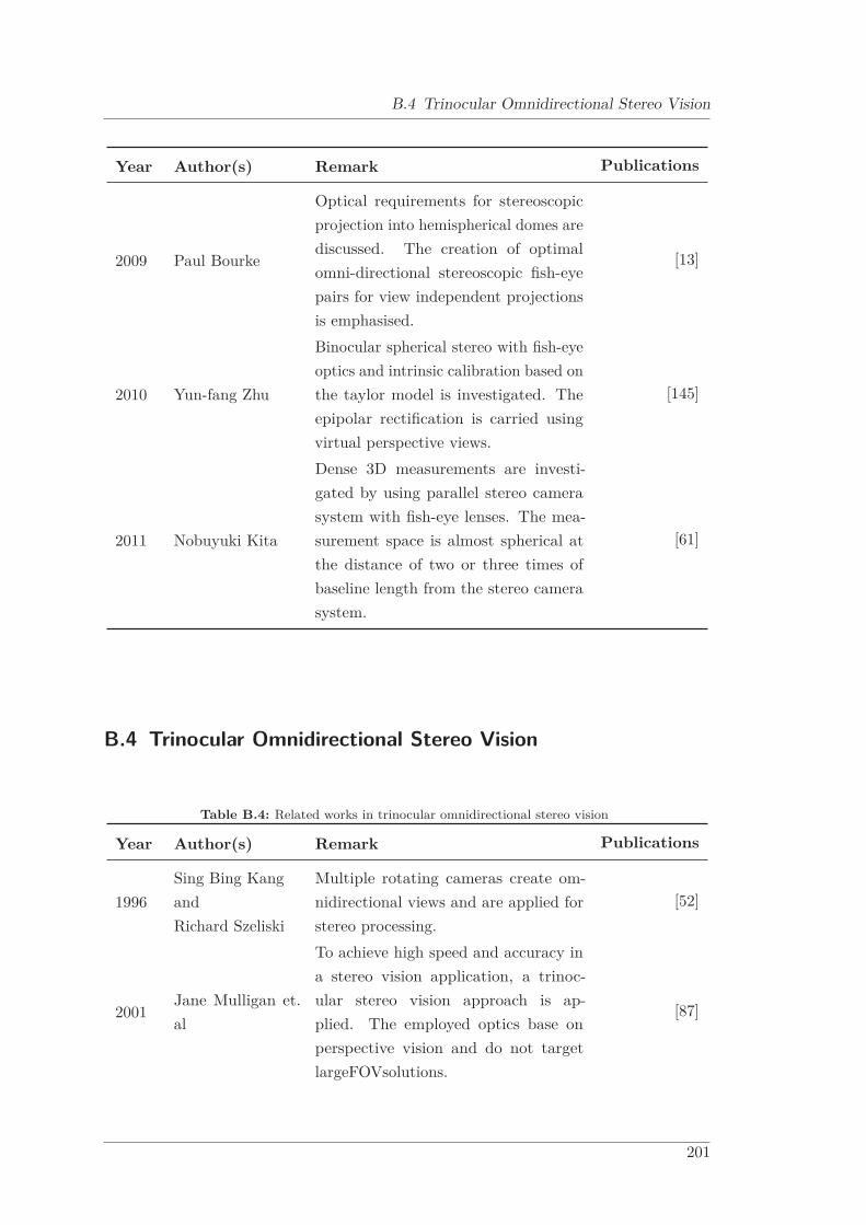
B.4 Trinocular Omnidirectional Stereo Vision
Year Author(s) Remark Publications
2009 Paul Bourke
Optical requirements for stereoscopicprojection into hemispherical domes arediscussed. The creation of optimalomni-directional stereoscopic fish-eyepairs for view independent projectionsis emphasised.
[13]
2010 Yun-fang Zhu
Binocular spherical stereo with fish-eyeoptics and intrinsic calibration based onthe taylor model is investigated. Theepipolar rectification is carried usingvirtual perspective views.
[145]
2011 Nobuyuki Kita
Dense 3D measurements are investi-gated by using parallel stereo camerasystem with fish-eye lenses. The mea-surement space is almost spherical atthe distance of two or three times ofbaseline length from the stereo camerasystem.
[61]
B.4 Trinocular Omnidirectional Stereo Vision
Table B.4: Related works in trinocular omnidirectional stereo vision
Year Author(s) Remark Publications
1996Sing Bing KangandRichard Szeliski
Multiple rotating cameras create om-nidirectional views and are applied forstereo processing.
[52]
2001Jane Mulligan et.al
To achieve high speed and accuracy ina stereo vision application, a trinoc-ular stereo vision approach is ap-plied. The employed optics base onperspective vision and do not targetlargeFOVsolutions.
[87]
201

Appendix B Further Relevant Publications
Year Author(s) Remark Publications
2006 Shigang Li
A trinocular spherical stereo vision ap-proach based on fisheye optics andlatitude-longitude sampling is pre-sented. Theoretically, a hemisphericaldepth map can be generated.
[67]
B.5 Miscellaneous Configurations
Table B.5: N-ocular omnidirectional stereo vision
Year Author(s) Remark Publications
199920012002
Kim C. Nga et. al
Multiple deployed omnidirectional vi-sion sensors are employed for 3D rang-ing and generation of virtual sceneviews.
[89–91]
200020012004
Hideki Tanahashiet. al
A stereo omnidirectional imaging sys-tem named SOS is presented. It consistsof multiple (e.g. 60) perspective cam-eras arranged as stereo units each ona face of a regular icosahedron. A fullspherical depth map can be obtained.
[112,122,123]
20002001
Takushi Sogo et.al
Multiple deployed catadioptric visionsensors form a n-ocular stereo systemfor real-time human tracking.
[116,117]
20092013
Hansung Kim andAdrian Hilton
For the purpose of 3D reconstructionmultiple spherical images are generatedby a bunch of rotating line cameras. A3D mesh model for each pair of spher-ical images is reconstructed by stereomatching.
[59,60]
2010Tomokazu Satoand NaokazuYokoya
A method is presented for estimatinga depth map from a calibrated movingomnidirectional multi-camera system.
[101]
202
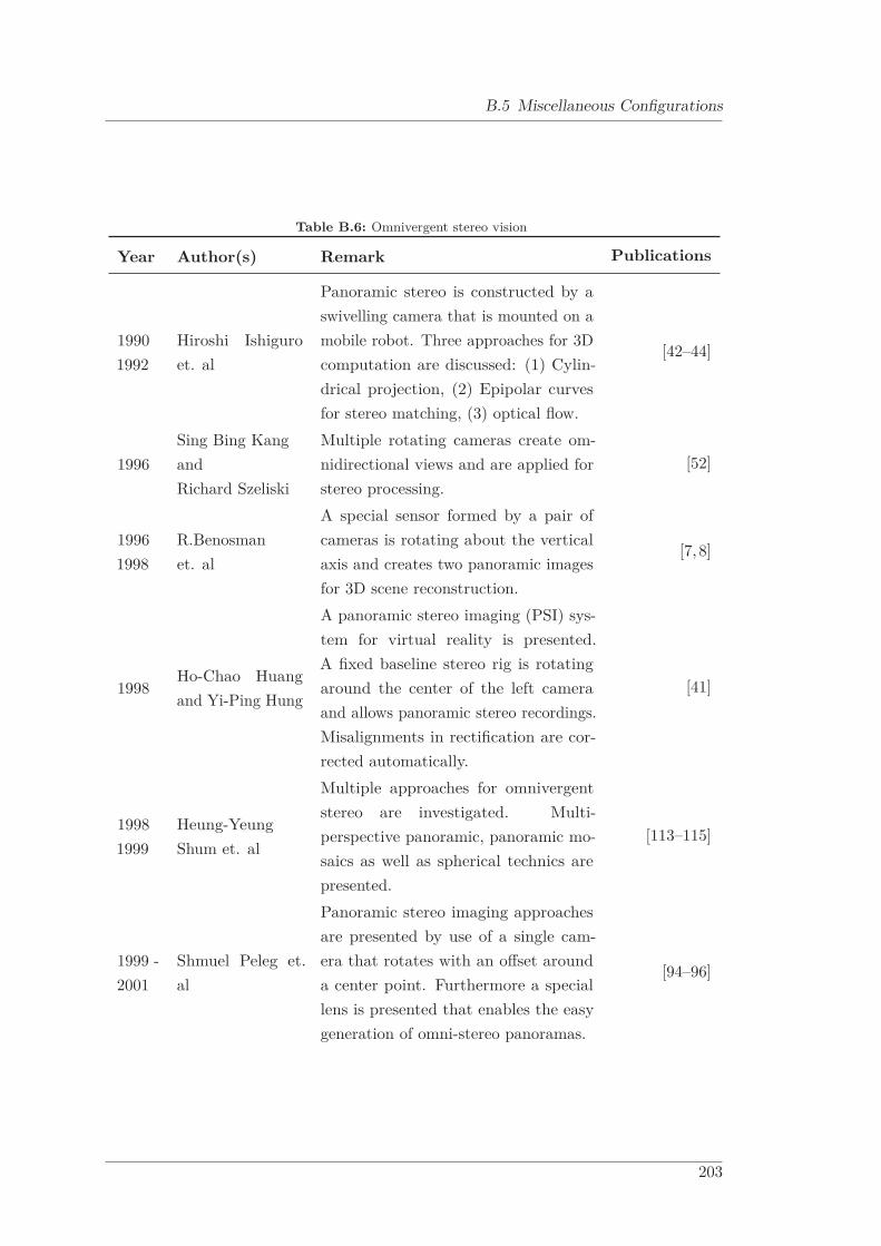
B.5 Miscellaneous Configurations
Table B.6: Omnivergent stereo vision
Year Author(s) Remark Publications
19901992
Hiroshi Ishiguroet. al
Panoramic stereo is constructed by aswivelling camera that is mounted on amobile robot. Three approaches for 3Dcomputation are discussed: (1) Cylin-drical projection, (2) Epipolar curvesfor stereo matching, (3) optical flow.
[42–44]
1996Sing Bing KangandRichard Szeliski
Multiple rotating cameras create om-nidirectional views and are applied forstereo processing.
[52]
19961998
R.Benosmanet. al
A special sensor formed by a pair ofcameras is rotating about the verticalaxis and creates two panoramic imagesfor 3D scene reconstruction.
[7, 8]
1998Ho-Chao Huangand Yi-Ping Hung
A panoramic stereo imaging (PSI) sys-tem for virtual reality is presented.A fixed baseline stereo rig is rotatingaround the center of the left cameraand allows panoramic stereo recordings.Misalignments in rectification are cor-rected automatically.
[41]
19981999
Heung-YeungShum et. al
Multiple approaches for omnivergentstereo are investigated. Multi-perspective panoramic, panoramic mo-saics as well as spherical technics arepresented.
[113–115]
1999 -2001
Shmuel Peleg et.al
Panoramic stereo imaging approachesare presented by use of a single cam-era that rotates with an offset arounda center point. Furthermore a speciallens is presented that enables the easygeneration of omni-stereo panoramas.
[94–96]
203

Appendix B Further Relevant Publications
Year Author(s) Remark Publications
2004Yin Liet. al
A large collection of images taken bycameras that move in concentric circlesis assembled to multiple panoramic im-ages. Successively they compute multi-perspective stereo vision.
[70]
2004Wei Jianget. al
A large collection of images taken bystereo cameras that move in concen-tric circles is assembled to multiplepanoramic images. The two collectionsof regular perspective images are resam-pled into four multi-perspective panora-mas. Afterwards depth information iscomputed using three types of epipo-lar constraints: horizontal, vertical andcombination of them.
[50]
20092013
Hansung Kim andAdrian Hilton
For the purpose of 3D reconstructionmultiple spherical images are generatedby a bunch of rotating line cameras. A3D mesh model for each pair of spher-ical images is reconstructed by stereomatching.
[59,60]
2010 Paul Bourke
By means of a single camera and a fish-eye lens, the capture of omni-directionalstereoscopic spherical projections is pre-sented. Furthermore the use of a singlecamera is compared to the employmentof two rotating cameras.
[12]
204
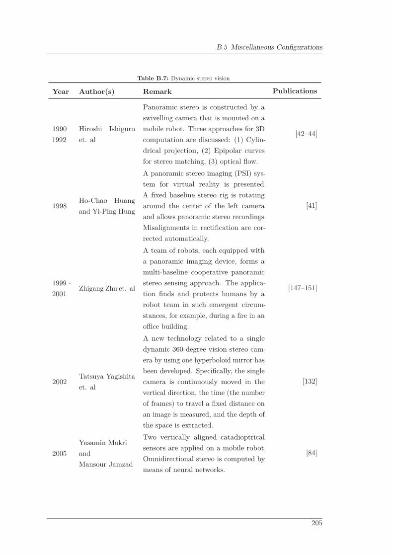
B.5 Miscellaneous Configurations
Table B.7: Dynamic stereo vision
Year Author(s) Remark Publications
19901992
Hiroshi Ishiguroet. al
Panoramic stereo is constructed by aswivelling camera that is mounted on amobile robot. Three approaches for 3Dcomputation are discussed: (1) Cylin-drical projection, (2) Epipolar curvesfor stereo matching, (3) optical flow.
[42–44]
1998Ho-Chao Huangand Yi-Ping Hung
A panoramic stereo imaging (PSI) sys-tem for virtual reality is presented.A fixed baseline stereo rig is rotatingaround the center of the left cameraand allows panoramic stereo recordings.Misalignments in rectification are cor-rected automatically.
[41]
1999 -2001
Zhigang Zhu et. al
A team of robots, each equipped witha panoramic imaging device, forms amulti-baseline cooperative panoramicstereo sensing approach. The applica-tion finds and protects humans by arobot team in such emergent circum-stances, for example, during a fire in anoffice building.
[147–151]
2002Tatsuya Yagishitaet. al
A new technology related to a singledynamic 360-degree vision stereo cam-era by using one hyperboloid mirror hasbeen developed. Specifically, the singlecamera is continuously moved in thevertical direction, the time (the numberof frames) to travel a fixed distance onan image is measured, and the depth ofthe space is extracted.
[132]
2005Yasamin MokriandMansour Jamzad
Two vertically aligned catadioptricalsensors are applied on a mobile robot.Omnidirectional stereo is computed bymeans of neural networks.
[84]
205

Appendix B Further Relevant Publications
Year Author(s) Remark Publications
2008Ryosuke Kawan-ishi et. al
A mobile robot equipped with a sin-gle omnidirectional camera acquires se-quences of images and computes the3D surrounding with a structure frommotion approach.
[58]
Table B.8: Omnidirectional stereo vision with special optical solutions
Year Author(s) Remark Publications
19962000
David Southwellet. al
Catadioptric cameras are equipped withspecial double lobbed mirrors in orderto perform stereoscopic measurementswith one single camera.
[6, 118]
1999 -2001
Shmuel Peleg et.al
Panoramic stereo imaging approachesare presented by use of a single cam-era that rotates with an offset arounda center point. Furthermore a speciallens is presented that enables the easygeneration of omni-stereo panoramas.
[94–96]
200020012004
Hideki Tanahashiet. al
A stereo omnidirectional imaging sys-tem named SOS is presented. It consistsof multiple (e.g. 60) perspective cam-eras arranged as stereo units each ona face of a regular icosahedron. A fullspherical depth map can be obtained.
[112,122,123]
2003Shih-Schon LinandRuzena Bajcsy
A novel catadioptric sensor for omni-directional stereo vision is presented.This sensor bases on two regular per-spective cameras, a beam splitter andone reflective surface.
[71]
2005Yuichiro Kojimaet. al
Catadioptric sensors in combinationwith special compound spherical mir-rors are applied in order to generate anomnidirectional 3D measurement sys-tem. An application is seen for instancein wearable security systems.
[62]
206
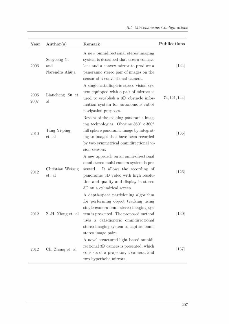
B.5 Miscellaneous Configurations
Year Author(s) Remark Publications
2006Sooyeong YiandNarendra Ahuja
A new omnidirectional stereo imagingsystem is described that uses a concavelens and a convex mirror to produce apanoramic stereo pair of images on thesensor of a conventional camera.
[134]
20062007
Liancheng Su et.al
A single catadioptric stereo vision sys-tem equipped with a pair of mirrors isused to establish a 3D obstacle infor-mation system for autonomous robotnavigation purposes.
[74, 121,144]
2010Tang Yi-pinget. al
Review of the existing panoramic imag-ing technologies. Obtains 360o × 360o
full sphere panoramic image by integrat-ing to images that have been recordedby two symmetrical omnidirectional vi-sion sensors.
[135]
2012Christian Weissiget. al
A new approach on an omni-directionalomni-stereo multi-camera system is pre-sented. It allows the recording ofpanoramic 3D video with high resolu-tion and quality and display in stereo3D on a cylindrical screen.
[126]
2012 Z.-H. Xiong et. al
A depth-space partitioning algorithmfor performing object tracking usingsingle-camera omni-stereo imaging sys-tem is presented. The proposed methoduses a catadioptric omnidirectionalstereo-imaging system to capture omni-stereo image pairs.
[130]
2012 Chi Zhang et. al
A novel structured light based omnidi-rectional 3D camera is presented, whichconsists of a projector, a camera, andtwo hyperbolic mirrors.
[137]
207


Bibliography
[1] Vision3D. http://www.vision3d.com/stereo.html, . – Accessed: 2015-01-27
[2] Abdel-Aziz, Y.I. ; Karara, H.M.: Direct linear transformation into object spacecoordinates in closerange photogrametry. In: Close-Range Photogrametry (1971),S. 1–18
[3] Abraham, Steffen ; Foerstner, Wolfgang: Fish-eye-stereo calibration andepipolar rectification. In: ISPRS Journal of Photogrammetry and Remote Sensing59 (2005), S. 278–288
[4] Amat, J. ; Frigola, M. ; Casals, A.: Selection of the best stereo pair in amulti-camera configuration. In: Robotics and Automation, 2002. Proceedings. ICRA’02. IEEE International Conference on Bd. 4, 2002, S. 3342–3346 vol.4
[5] Ardouin, Jérôme ; Lécuyer, Anatole ; Marchal, Maud ; Riant, Clément ;Marchand, Eric: FlyVIZ: a novel display device to provide humans with 360degree vision by coupling catadioptric camera with hmd. In: Proceedings of the18th ACM symposium on Virtual reality software and technology. New York, NY,USA : ACM, 2012 (VRST ’12). – ISBN 978–1–4503–1469–5, 41–44
[6] Baldwin, Jonathan ; Basu, Anup: 3D estimation using panoramic stereo. In:Pattern Recognition, 2000. Proceedings. 15th International Conference on Bd. 1,2000. – ISSN 1051–4651, S. 97–100 vol.1
[7] Benosman, R. ; Devars, J.: Panoramic stereo vision sensor. In: PatternRecognition, 1998. Proceedings. Fourteenth International Conference on Bd. 1, 1998.– ISSN 1051–4651, S. 767–769 vol.1
[8] Benosman, R. ; Maniere, T. ; Devars, J.: Real time omni-directional stereovisionand planes detection. In: Electrotechnical Conference, 1996. MELECON ’96., 8thMediterranean Bd. 2, 1996, S. 1151–1155 vol.2
[9] Blostein, S.D. ; Huang, T.S.: Error Analysis in Stereo Determination of 3-DPoint Positions. In: Pattern Analysis and Machine Intelligence, IEEE Transactionson PAMI-9 (1987), Nr. 6, S. 752–765. – ISSN 0162–8828
209

Bibliography
[10] Bo, Zhang ; Haitao, Xu ; Lulu, Lin ; Jun, Jiang ; Jianyue, Zhang ; Yiping, Tang:Development of Coordinate-machine of the Scene of Road Traffic Accident basedon Binocular Stereo Omni-Directional Vision Sensors. In: Procedia Engineering24 (2011), Nr. 0, S. 262 – 266. – ISSN 1877–7058. – International Conference onAdvances in Engineering 2011
[11] Bouguet, Jean-Yves: Camera calibration toolbox for matlab. (2004). http://www.vision.caltech.edu/bouguetj/calib_doc/index.html
[12] Bourke, P.: Capturing omni-directional stereoscopic spherical projections with asingle camera. In: Virtual Systems and Multimedia (VSMM), 2010 16th Interna-tional Conference on, 2010, S. 179–183
[13] Bourke, Paul: Omni-Directional stereoscopic fisheye images for immersive hemi-spherical dome environments. In: Comput. Games Allied Technol (2009), S. 136–143
[14] Bowman, Adrian W. ; Azzalini, Adelchi: Applied smoothing techniques for dataanalysis. Clarendon Press, 2004
[15] Braeuer-Burchardt, Christian ; Voss, Klaus: A new algorithm to correctfish-eye- and strong wide-angle-lens-distortion from single images. In: Proceedingsof the 2001 International Conference on Image Processing 1 (2001), S. 225–228
[16] Brown, D.C.: Decentering distortion of lenses. In: Photogrammetric Eng. RemoteSensing (1966), S. 444–462
[17] Chang, C. ; Chatterjee, S.: Quantization error analysis in stereo vision. In:Signals, Systems and Computers, 1992. 1992 Conference Record of The Twenty-Sixth Asilomar Conference on, 1992. – ISSN 1058–6393, S. 1037–1041 vol.2
[18] Csurka, Gabriella ; Zeller, Cyril ; Zhang, Zhengyou ; Faugeras, Olivier D.:Characterizing the Uncertainty of the Fundamental Matrix. In: Computer Visionand Image Understanding 68 (1997), Nr. 1, S. 18 – 36. – ISSN 1077–3142
[19] Devernay ; Faugeras: Straight Lines Have to Be Straight: Automatic Calibrationand Removal of Distortion from Scenes of Structured Environments. In: MachineVision and Applications 1 (2001), S. 14–24
[20] Dollár, P. ; Tu, Z. ; Perona, P. ; Belongie, S.: Integral Channel Features. In:BMVC, 2009
[21] Faugeras, Oliver: Three dimensional computer vision: A geometric viewpoint.the MIT Press, 1993
[22] Faugeras, Olivier ; Toscani, Giorgio: Camera calibration for 3D computer vision.In: International Workshop on Machine Vision and Machine Intelligence (1987), S.240–247
210

Bibliography
[23] Findeisen, M. ; Meinel, L. ; Hirtz, G.: A trinocular omnidirectional stereovision system for high-precision RGB-D acquisition. In: ELMAR (ELMAR), 201456th International Symposium, 2014, S. 1–4
[24] Findeisen, Michel ; Hirtz, Gangolf: Trinocular Spherical Stereo Vision for IndoorSurveillance. In: 11th Conference on Computer and Robot Vision (CRV). Montreal,Quebec, Canada : IEEE Xplore Digital Library, May 2014
[25] Findeisen, Michel ; Meinel, Lars ; Heß, Markus ; Apitzsch, André ; Hirtz,Gangolf: A Fast Approach For Omnidirectional Surveillance With Multiple VirtualPerspective Views. In: 2013 IEEE Eurocon International conference on computeras a tool. Zagreb, Croatia, 2013, S. 1578–1585
[26] Findeisen, Michel ; Meinel, Lars ; Richter, Julia ; Hirtz, Gangolf: AnOmnidirectional Stereo Sensor for Human Behavior Analysis in Complex IndoorEnvironments IEEE International Conference on Consumer Electronics, Las Vegas,2015
[27] Fooladgar, F. ; Samavi, S. ; Soroushmehr, S.M.R. ; Shirani, S.: GeometricalAnalysis of Localization Error in Stereo Vision Systems. In: Sensors Journal, IEEE13 (2013), Nr. 11, S. 4236–4246. – ISSN 1530–437X
[28] Fusiello, Andrea ; Trucco, Emanuele ; Verri, Alessandro: A compact algo-rithm for rectification of stereo pairs. In: Machine Vision and Applications 12(2000), Nr. 1, S. 16–22. http://dx.doi.org/10.1007/s001380050120. – DOI10.1007/s001380050120. – ISSN 0932–8092
[29] Ganapathy, S.: Decomposition of transformation matrices for robot vision. In:Proceedings of the 1984 IEEE International Conferece on Robotics and Automation(1984), S. 130–139
[30] Gandhi, Tarak: Motion analysis of omni-directional video streams for a mobilesentry. In: ACM International Workshop on Video Surveillance, ACM Press, 2003,S. 49–58
[31] Gluckman, Joshua ; Nayar, Shree K. ; Thoresz, Keith J.: Real-time omnidirec-tional and panoramic stereo. In: Proc. of DARPA Image Understanding WorkshopBd. 1, 1998, S. 299–303
[32] Hanning, Tobias: Re-projective calibration of a stereo camera system. In:International Conference on Visualization, Imaging and Image Processing (VIIP),2006, S. 7–12
[33] Hanning, Tobias: High precision camera calibration. Springer, 2011
211

Bibliography
[34] Hanning, Tobias ; Graf, Simone ; Pisinger, Georg: Extrinsic calibration of astereo camera system fulfilling generalized epipolar constraints. In: InternationalConference on Visualization, Imaging and Image Processing Conference (VIIP),2004, S. 1–5
[35] Hartley, Richard: Theory and practice of projective rectification. In: Interna-tional Journal of Computer Vision 35 (1999), Nr. 2, S. 115–127
[36] Hartley, Richard ; Zisserman, Andrew: Multiple view geometry in computervision. Bd. 2. Cambridge Univ Press, 2000
[37] Hartley, Richard ; Zisserman, Andrew: Multiple view geometry in computervision. Cambridge university press, 2003
[38] Heikkilä, Janne: Geometric Camera Calibration Using Circular Control Points.In: IEEE Transactions on Pattern Analysis and Machine Intelligence 22 (2000), S.1066–1077
[39] Heikkilä, Janne ; Silvén, Olli: A Four-step Camera Calibration Procedure withImplicit Image Correction. In: CVPR ’97 Proceedings of the 1997 Conference onComputer Vision and Pattern Recognition (1997)
[40] Hirschmuller, H. ; Scharstein, D.: Evaluation of Cost Functions for StereoMatching. In: Computer Vision and Pattern Recognition, 2007. CVPR ’07. IEEEConference on, 2007. – ISSN 1063–6919, S. 1–8
[41] Huang, Ho-Chao ; Hung, Yi-Ping: Panoramic stereo imaging system with auto-matic disparity warping and seaming. In: Graphical Models and Image Processing60 (1998), Nr. 3, S. 196–208
[42] Ishiguro, Hiroshi ; Yamamoto, Masashi ; Tsuji, Saburo: Analysis of omni-directional views at different location. In: Intelligent Robots and Systems ’90.’Towards a New Frontier of Applications’, Proceedings. IROS ’90. IEEE Interna-tional Workshop on, 1990, S. 659–664 vol.2
[43] Ishiguro, Hiroshi ; Yamamoto, Masashi ; Tsuji, Saburo: Omni-directionalstereo for making global map. In: Computer Vision, 1990. Proceedings, ThirdInternational Conference on, 1990, S. 540–547
[44] Ishiguro, Hiroshi ; Yamamoto, Masashi ; Tsuji, Saburo: Omni-directionalstereo. In: Pattern Analysis and Machine Intelligence, IEEE Transactions on14 (1992), Nr. 2, S. 257–262. http://dx.doi.org/10.1109/34.121792. – DOI10.1109/34.121792. – ISSN 0162–8828
212

Bibliography
[45] Ishii, C. ; Sudo, Y. ; Hashimoto, H.: An image conversion algorithm from fish eyeimage to perspective image for human eyes. In: Advanced Intelligent Mechatronics,2003. AIM 2003. Proceedings. 2003 IEEE/ASME International Conference onBd. 2, 2003, S. 1009–1014 vol.2
[46] Jaehne, Bernd: Digitale Bildverarbeitung. Springer DE, 2012
[47] Jeng, S. W. ; Tsai, W.H.: Using pano-mapping tables for unwarping of omni-images into panoramic and perspective-view images. In: Image Processing, IET 1(2007), June, Nr. 2, S. 149–155. http://dx.doi.org/10.1049/iet-ipr:20060201.– DOI 10.1049/iet–ipr:20060201. – ISSN 1751–9659
[48] Jeng, Sheng-Wen ; Tsai, Wen-Hsiang: Construction of perspective and panoramicimages from omni-images taken from hypercatadioptric cameras for visual surveil-lance. In: Networking, Sensing and Control, 2004 IEEE International Conferenceon Bd. 1, 2004. – ISSN 1810–7869, S. 204–209 Vol.1
[49] Jeng, Sheng-Wen ; Tsai, Wen-Hsiang: Analytic image unwarping by a systematiccalibration method for omni-directional cameras with hyperbolic-shaped mirrors.In: Image and Vision Computing 26 (2008), Nr. 5, S. 690 – 701. – ISSN 0262–8856
[50] Jiang, Wei ; Sugimoto, S. ; Okutomi, M.: Omnidirectional 3D reconstructionusing stereo multi-perspective panoramas. In: SICE 2004 Annual Conference Bd. 2,2004, S. 1128–1133 vol. 2
[51] Kaden, Sascha: Merging Depth Maps from the Omnidirectional Stereo Vision /Chemnitz University of Technology, Professorship Digital Signal Processing andCircuit Technology. 2014. – Forschungsbericht
[52] Kang, Sing B. ; Szeliski, R.: 3-D scene data recovery using omnidirectional multi-baseline stereo. In: Computer Vision and Pattern Recognition, 1996. ProceedingsCVPR ’96, 1996 IEEE Computer Society Conference on, 1996. – ISSN 1063–6919,S. 364–370
[53] Kannala, Juho: Camera Calibration Toolbox for Generic Lenses. http://www.ee.oulu.fi/~jkannala/calibration/calibration.html. Version: 2008
[54] Kannala, Juho: Models and methods for geometric computer vision. In: Academicdissertation (2010)
[55] Kannala, Juho ; Brandt, Sami S.: A Generic Camera Calibration Method forFish-Eye Lenses. In: Proceedings of the 17th International Conference on PatternRecognition (ICPR) (2004)
213

Bibliography
[56] Kannala, Juho ; Brandt, Sami S.: A generic camera model and calibrationmethod for conventional, wide-angle, and fish-eye lenses. In: Pattern Analysis andMachine Intelligence, IEEE Transactions on 28 (2006), Aug, Nr. 8, S. 1335–1340.http://dx.doi.org/10.1109/TPAMI.2006.153. – DOI 10.1109/TPAMI.2006.153.– ISSN 0162–8828
[57] Kannala, Juho ; Heikkila, Janne ; Brandt, Sami S.: Geometric CameraCalibration. In: Wiley Encyclopedia of Computer Science and Engineering (2008)
[58] Kawanishi, Ryosuke ; Yamashita, Atsushi ; Kaneko, Toru: Construction of3D Environment Model from an Omni-Directional Image Sequence. In: AsiaInternational Symposium on Mechatronics, 2008
[59] Kim, Hansung ; Hilton, A.: Environment modelling using spherical stereo imaging.In: Computer Vision Workshops (ICCV Workshops), 2009 IEEE 12th InternationalConference on, 2009, S. 1534–1541
[60] Kim, Hansung ; Hilton, Adrian: 3D Scene Reconstruction from Multiple SphericalStereo Pairs. In: International Journal of Computer Vision 104 (2013), Nr. 1, S.94–116. – ISSN 0920–5691
[61] Kita, Nobuyuki: Dense 3D Measurement of the Near Surroundings by FisheyeStereo. In: Proc. The Twelfth IAPR Conference on Machine Vision Applications,2011
[62] Kojima, Yuichiro ; Sagawa, Ryusuke ; Echigo, Tomio ; Yagi, Yasushi: Cali-bration and Performance Evaluation of Omnidirectional Sensor with CompoundSpherical Mirrors. In: IPSJ SIG Technical Reports Bd. 38, 2005, S. 31–38
[63] Kwon, Hyukseong ; Park, Johnny ; Kak, Avinash C.: A New Approach for ActiveStereo Camera Calibration. In: Robotics and Automation, 2007 IEEE InternationalConference on, 2007. – ISSN 1050–4729, S. 3180–3185
[64] Lenz, R.K. ; Tsai, R.Y.: Techniques for calibration of the scale factor and imagecenter for high accuracy 3D machine vision metrology. In: Proceedings of the IEEEInternational Conference on Robotics Automation (1987), S. 68–75
[65] Li, Fuxing ; Brady, Michael ; Wiles, Charles: Fast computation of thefundamental matrix for an active stereo vision system. Version: 1996. http://dx.doi.org/10.1007/BFb0015532. In: Buxton, Bernard (Hrsg.) ; Cipolla,Roberto (Hrsg.): Computer Vision - ECCV ’96 Bd. 1064. Springer Berlin Heidel-berg, 1996. – DOI 10.1007/BFb0015532. – ISBN 978–3–540–61122–6, 157-166
[66] Li, Shigang: Real-Time Spherical Stereo. In: Pattern Recognition, 2006. ICPR2006. 18th International Conference on Bd. 3, 2006. – ISSN 1051–4651, S. 1046–1049
214

Bibliography
[67] Li, Shigang: Trinocular Spherical Stereo. In: Intelligent Robots and Systems, 2006IEEE/RSJ International Conference on, 2006, S. 4786–4791
[68] Li, Shigang: Binocular Spherical Stereo. In: Intelligent Transportation Systems,IEEE Transactions on 9 (2008), Nr. 4, S. 589–600. http://dx.doi.org/10.1109/TITS.2008.2006736. – DOI 10.1109/TITS.2008.2006736. – ISSN 1524–9050
[69] Li, Shigang ; Fukumori, Kiyotaka: Spherical stereo for the construction ofimmersive VR environment. In: Virtual Reality, 2005. Proceedings. VR 2005.IEEE, 2005, S. 217–222
[70] Li, Yin ; Shum, Heung-Yeung ; Tang, Chi-Keung ; Szeliski, R.: Stereo recon-struction from multiperspective panoramas. In: Pattern Analysis and MachineIntelligence, IEEE Transactions on 26 (2004), Nr. 1, S. 45–62. http://dx.doi.org/10.1109/TPAMI.2004.1261078. – DOI 10.1109/TPAMI.2004.1261078. – ISSN0162–8828
[71] Lin, Shih-Schon ; Bajcsy, Ruzena: High resolution catadioptric omni-directionalstereo sensor for robot vision. In: Robotics and Automation, 2003. Proceedings.ICRA ’03. IEEE International Conference on Bd. 2, 2003. – ISSN 1050–4729, S.1694–1699 vol.2
[72] Longuet-Higgins, H. C.: A computer algorithm for reconstructing a scene fromtwo projections. In: Readings in Computer Vision: Issues, Problems, Principles,and Paradigms, MA Fischler and O. Firschein, eds (1987), S. 61–62
[73] Loop, Charles ; Zhang, Zhengyou: Computing rectifying homographies for stereovision. In: Computer Vision and Pattern Recognition, 1999. IEEE ComputerSociety Conference on. Bd. 1, 1999. – ISSN 1063–6919, S. –131 Vol. 1
[74] Luo, Chuanjiang ; Su, Liancheng ; Zhu, Feng: A novel omnidirectional stereovision system via a single camera. In: Scene Reconstruction Pose Estimation andTracking, InTech (2007), S. 19–38
[75] Luong, Quan-Tuan ; Faugeras, Olivier D.: The fundamental matrix: Theory,algorithms, and stability analysis. In: International Journal of Computer Vision17 (1996), Nr. 1, S. 43–75
[76] Matousek, Martin ; Sara, Radim ; Hlavac, Vaclav: Data-optimal rectificationfor fast and accurate stereovision. In: Multi-Agent Security and Survivability, 2004IEEE First Symposium on, 2004, S. 212–215
[77] Mattoccia, Stefano: Stereo Vision: Algorithms and Applications. October 2013
215

Bibliography
[78] McMillan, Leonard ; Bishop, Gary: Plenoptic modeling: an image-basedrendering system. In: Proceedings of the 22nd annual conference on Computergraphics and interactive techniques. New York, NY, USA : ACM, 1995 (SIGGRAPH’95). – ISBN 0–89791–701–4, S. 39–46
[79] Meinel, Lars: Verfahren zur Kalibrierung von perspektivischen und omnidirek-tionalen Kamerasystemen, Chemnitz University of Technology, Diplomarbeit, 2012
[80] Meinel, Lars: Multi-Objektverfolgung zur Innenraumüberwachung unter Nutzungeines omnidirektionalen Kamerasystems, Chemnitz University of Technology, Diplo-marbeit, 2013
[81] Meinel, Lars ; Findeisen, Michel ; Heß, Markus ; Apitzsch, André ; Hirtz,Gangolf: Automated Real-Time Surveillance for Ambient Assisted Living Using anOmnidirectional Camera. In: 2014 IEEE International Conference on ConsumerElectronics (ICCE) (2014 IEEE ICCE). Las Vegas, USA, Januar 2014, S. 402–405
[82] Meinel, Lars ; Wiede, Christian ; Findeisen, Michel ; Apitzsch, Andre ;Hirtz, Gangolf: Virtual perspective views for real-time people detection using anomnidirectional camera. In: Imaging Systems and Techniques (IST), 2014 IEEEInternational Conference on, 2014, S. 312–315
[83] Melen, Trond: Geometrical Modelling and Calibration of Video Cameras forUnderwater Navigation. In: Dissertation zum Dr.-Ing., Univ. of Science andTechnology, Trondheim, Norwegen (1994)
[84] Mokri, Yasamin ; Jamzad, Mansour: Omni-stereo vision system for an au-tonomous robot using neural networks. In: Electrical and Computer Engineering,2005. Canadian Conference on, 2005. – ISSN 0840–7789, S. 1590–1593
[85] Monasse, Pascal ; Morel, Jean-Michel ; Tang, Zhongwei: Three-step imagerectification. In: Proceedings of the British Machine Vision Conference, 2010
[86] Mouaddib, El M. ; Sagawa, Ryusuke ; Echigo, Tomio ; Yagi, Yasushi: Two ormore mirrors for the omnidirectional stereovision? In: eurasip 52 (2006)
[87] Mulligan, Jane ; Isler, Volkan ; Daniilidis, Kostas: Trinocular stereo: areal-time algorithm and its evaluation. In: Stereo and Multi-Baseline Vision, 2001.(SMBV 2001). Proceedings. IEEE Workshop on, 2001, S. 10–17
[88] Nene, S.A. ; Nayar, S.K.: Stereo with mirrors. In: Computer Vision, 1998. SixthInternational Conference on, 1998, S. 1087–1094
[89] Ng, Kim C. ; Trivedi, Mohan M. ; Ishigurob, Hiroshi: 3 D ranging andvirtual view generation using omni-view cameras. In: Proceedings of SPIE- TheInternational Society for Optical Engineering Bd. 3528, 1999, S. 11–14
216
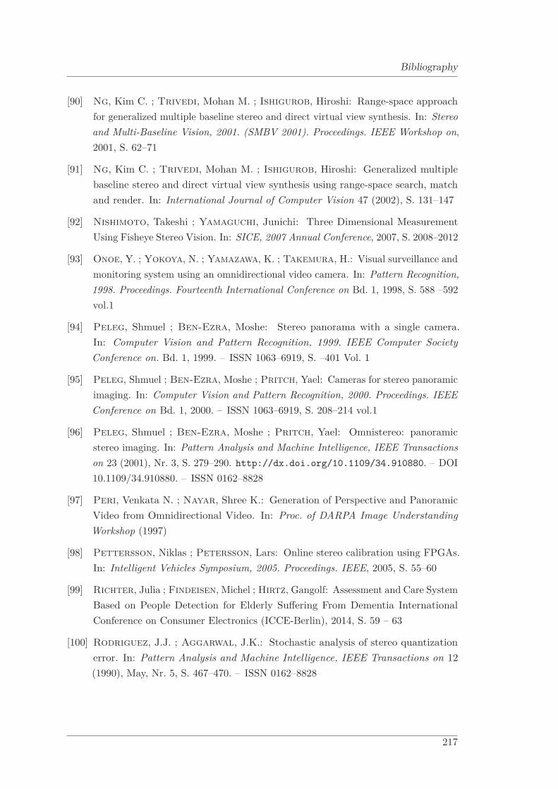
Bibliography
[90] Ng, Kim C. ; Trivedi, Mohan M. ; Ishigurob, Hiroshi: Range-space approachfor generalized multiple baseline stereo and direct virtual view synthesis. In: Stereoand Multi-Baseline Vision, 2001. (SMBV 2001). Proceedings. IEEE Workshop on,2001, S. 62–71
[91] Ng, Kim C. ; Trivedi, Mohan M. ; Ishigurob, Hiroshi: Generalized multiplebaseline stereo and direct virtual view synthesis using range-space search, matchand render. In: International Journal of Computer Vision 47 (2002), S. 131–147
[92] Nishimoto, Takeshi ; Yamaguchi, Junichi: Three Dimensional MeasurementUsing Fisheye Stereo Vision. In: SICE, 2007 Annual Conference, 2007, S. 2008–2012
[93] Onoe, Y. ; Yokoya, N. ; Yamazawa, K. ; Takemura, H.: Visual surveillance andmonitoring system using an omnidirectional video camera. In: Pattern Recognition,1998. Proceedings. Fourteenth International Conference on Bd. 1, 1998, S. 588 –592vol.1
[94] Peleg, Shmuel ; Ben-Ezra, Moshe: Stereo panorama with a single camera.In: Computer Vision and Pattern Recognition, 1999. IEEE Computer SocietyConference on. Bd. 1, 1999. – ISSN 1063–6919, S. –401 Vol. 1
[95] Peleg, Shmuel ; Ben-Ezra, Moshe ; Pritch, Yael: Cameras for stereo panoramicimaging. In: Computer Vision and Pattern Recognition, 2000. Proceedings. IEEEConference on Bd. 1, 2000. – ISSN 1063–6919, S. 208–214 vol.1
[96] Peleg, Shmuel ; Ben-Ezra, Moshe ; Pritch, Yael: Omnistereo: panoramicstereo imaging. In: Pattern Analysis and Machine Intelligence, IEEE Transactionson 23 (2001), Nr. 3, S. 279–290. http://dx.doi.org/10.1109/34.910880. – DOI10.1109/34.910880. – ISSN 0162–8828
[97] Peri, Venkata N. ; Nayar, Shree K.: Generation of Perspective and PanoramicVideo from Omnidirectional Video. In: Proc. of DARPA Image UnderstandingWorkshop (1997)
[98] Pettersson, Niklas ; Petersson, Lars: Online stereo calibration using FPGAs.In: Intelligent Vehicles Symposium, 2005. Proceedings. IEEE, 2005, S. 55–60
[99] Richter, Julia ; Findeisen, Michel ; Hirtz, Gangolf: Assessment and Care SystemBased on People Detection for Elderly Suffering From Dementia InternationalConference on Consumer Electronics (ICCE-Berlin), 2014, S. 59 – 63
[100] Rodriguez, J.J. ; Aggarwal, J.K.: Stochastic analysis of stereo quantizationerror. In: Pattern Analysis and Machine Intelligence, IEEE Transactions on 12(1990), May, Nr. 5, S. 467–470. – ISSN 0162–8828
217
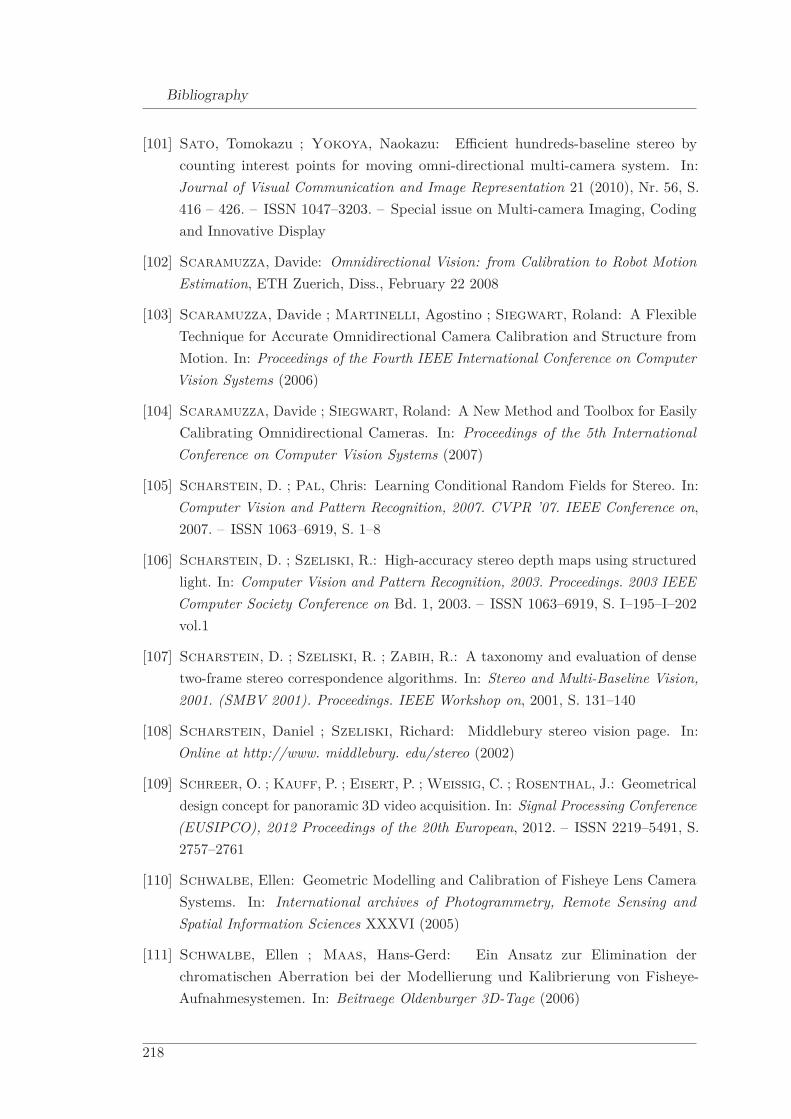
Bibliography
[101] Sato, Tomokazu ; Yokoya, Naokazu: Efficient hundreds-baseline stereo bycounting interest points for moving omni-directional multi-camera system. In:Journal of Visual Communication and Image Representation 21 (2010), Nr. 56, S.416 – 426. – ISSN 1047–3203. – Special issue on Multi-camera Imaging, Codingand Innovative Display
[102] Scaramuzza, Davide: Omnidirectional Vision: from Calibration to Robot MotionEstimation, ETH Zuerich, Diss., February 22 2008
[103] Scaramuzza, Davide ; Martinelli, Agostino ; Siegwart, Roland: A FlexibleTechnique for Accurate Omnidirectional Camera Calibration and Structure fromMotion. In: Proceedings of the Fourth IEEE International Conference on ComputerVision Systems (2006)
[104] Scaramuzza, Davide ; Siegwart, Roland: A New Method and Toolbox for EasilyCalibrating Omnidirectional Cameras. In: Proceedings of the 5th InternationalConference on Computer Vision Systems (2007)
[105] Scharstein, D. ; Pal, Chris: Learning Conditional Random Fields for Stereo. In:Computer Vision and Pattern Recognition, 2007. CVPR ’07. IEEE Conference on,2007. – ISSN 1063–6919, S. 1–8
[106] Scharstein, D. ; Szeliski, R.: High-accuracy stereo depth maps using structuredlight. In: Computer Vision and Pattern Recognition, 2003. Proceedings. 2003 IEEEComputer Society Conference on Bd. 1, 2003. – ISSN 1063–6919, S. I–195–I–202vol.1
[107] Scharstein, D. ; Szeliski, R. ; Zabih, R.: A taxonomy and evaluation of densetwo-frame stereo correspondence algorithms. In: Stereo and Multi-Baseline Vision,2001. (SMBV 2001). Proceedings. IEEE Workshop on, 2001, S. 131–140
[108] Scharstein, Daniel ; Szeliski, Richard: Middlebury stereo vision page. In:Online at http://www. middlebury. edu/stereo (2002)
[109] Schreer, O. ; Kauff, P. ; Eisert, P. ; Weissig, C. ; Rosenthal, J.: Geometricaldesign concept for panoramic 3D video acquisition. In: Signal Processing Conference(EUSIPCO), 2012 Proceedings of the 20th European, 2012. – ISSN 2219–5491, S.2757–2761
[110] Schwalbe, Ellen: Geometric Modelling and Calibration of Fisheye Lens CameraSystems. In: International archives of Photogrammetry, Remote Sensing andSpatial Information Sciences XXXVI (2005)
[111] Schwalbe, Ellen ; Maas, Hans-Gerd: Ein Ansatz zur Elimination derchromatischen Aberration bei der Modellierung und Kalibrierung von Fisheye-Aufnahmesystemen. In: Beitraege Oldenburger 3D-Tage (2006)
218
Bibliography
[112] Shimizu, Sanae ; Yamamoto, Kazuhiko ; Wang, Caihua ; Satoh, Yutaka; Tanahashi, Hideki ; Niwa, Yoshinori: Moving object detection by mobileStereo Omni-directional System (SOS) using spherical depth image. In: PatternRecognition, 2004. ICPR 2004. Proceedings of the 17th International Conferenceon Bd. 3, 2004. – ISSN 1051–4651, S. 248–251 Vol.3
[113] Shum, Heung-Yeung ; Han, Mei ; Szeliski, Richard: Interactive construction of3D models from panoramic mosaics. In: Computer Vision and Pattern Recognition,1998. Proceedings. 1998 IEEE Computer Society Conference on, 1998. – ISSN1063–6919, S. 427–433
[114] Shum, Heung-Yeung ; Kalai, Adam ; Seitz, Steven M.: Omnivergent stereo.In: Computer Vision, 1999. The Proceedings of the Seventh IEEE InternationalConference on Bd. 1, 1999, S. 22–29 vol.1
[115] Shum, Heung-Yeung ; Szeliski, Richard: Stereo reconstruction from multiperspec-tive panoramas. In: Computer Vision, 1999. The Proceedings of the Seventh IEEEInternational Conference on Bd. 1, 1999, S. 14–21 vol.1
[116] Sogo, T. ; Ishiguro, H. ; Trivedi, M.M.: N-Ocular Stereo for Real-Time HumanTracking. In: Benosman, Ryad (Hrsg.) ; Kang, SingBing (Hrsg.): PanoramicVision. Springer New York, 2001 (Monographs in Computer Science). – ISBN978–1–4419–2880–1, S. 359–375
[117] Sogo, Takushi ; Ishiguro, Hiroshi ; Trivedi, Mohan M.: Real-Time TargetLocalization and Tracking by N-Ocular Stereo. In: Omnidirectional Vision, 2000.Proceedings. IEEE Workshop on, 2000, S. 153–160
[118] Southwell, David ; Basu, Anup ; Fiala, Mark ; Reyda, Jereome: Panoramicstereo. In: Pattern Recognition, 1996., Proceedings of the 13th InternationalConference on Bd. 1, 1996. – ISSN 1051–4651, S. 378–382 vol.1
[119] Sturm, Peter: Mixing catadioptric and perspective cameras. In: OmnidirectionalVision, 2002. Proceedings. Third Workshop on IEEE, 2002, S. 37–44
[120] Su, Huihuang ; He, Bingwei: Stereo rectification of calibrated image pairs basedon geometric transformation. In: International Journal of Modern Education andComputer Science (IJMECS) 3 (2011), Nr. 4, S. 17
[121] Su, Liancheng ; Luo, Chuanjiang ; Zhu, Feng: Obtaining Obstacle Information byan Omnidirectional Stereo Vision System. In: Information Acquisition, 2006 IEEEInternational Conference on, 2006, S. 48–52
219

Bibliography
[122] Tanahashi, Hideki ; Niwa, Yoshinori ; Wang, Caihua ; Niwa, Yoshinori: Develop-ment of a stereo omnidirectional imaging system (SOS). In: Industrial ElectronicsSociety, 2000. IECON 2000. 26th Annual Confjerence of the IEEE Bd. 1, 2000, S.289–294 vol.1
[123] Tanahashi, Hideki ; Niwa, Yoshinori ; Wang, Caihua ; Niwa, Yoshinori: Acqui-sition of three-dimensional information in a real environment by using the StereoOmni-directional System (SOS). In: 3-D Digital Imaging and Modeling, 2001.Proceedings. Third International Conference on, 2001, S. 365–371
[124] Thibault, Simon: Enhanced surveillance system based on panomorph panoramiclenses. In: Defense and Security Symposium International Society for Optics andPhotonics, 2007, S. 65400E–65400E
[125] Tsai, Roger Y.: A Versatile Camera Calibration Techniaue for High-Accuracy 3DMachine Vision Metrology Using Off-the-shelf TV Cameras and Lenses. In: IEEEJOURNAL OF ROBOTICS AND AUTOMATION RS-3 (1987), S. 323–344
[126] Weissig, Christian ; Schreer, Oliver ; Eisert, Peter ; Kauff, Peter: The Ulti-mate Immersive Experience: Panoramic 3D Video Acquisition. In: Schoeffmann,Klaus (Hrsg.) ; Merialdo, Bernard (Hrsg.) ; Hauptmann, AlexanderG. (Hrsg.); Ngo, Chong-Wah (Hrsg.) ; Andreopoulos, Yiannis (Hrsg.) ; Breiteneder,Christian (Hrsg.): Advances in Multimedia Modeling Bd. 7131. Springer BerlinHeidelberg, 2012. – ISBN 978–3–642–27354–4, S. 671–681
[127] Weng, Juyang ; Cohen, Paul ; Herniou, Marc: Calibration of stereo camerasusing a non-linear distortion model. In: Pattern Recognition, 1990. Proceedings.,10th International Conference on Bd. i, 1990, S. 246–253 vol.1
[128] Weng, Juyang ; Cohen, Paul ; Herniou, Marc: Camera Calibration withDistortion Models and Accuracy Evaluation. In: IEEE Transactions on PatternAnalysis and Machine Intelligence 14 (1992), S. 965–980
[129] Wong, K.M.: Mathematical formulation and digital analysis in closerange pho-togrammetry. In: Photogrammetric Eng. Remote Sensing 41 (1975), S. 1355–1373
[130] Xiong, Z.-H. ; Cheng, I. ; Chen, W. ; Basu, A. ; Zhang, M.-J.: Depth spacepartitioning for omni-stereo object tracking. In: Computer Vision, IET 6 (2012),Nr. 2, S. 153–163. http://dx.doi.org/10.1049/iet-cvi.2010.0115. – DOI10.1049/iet–cvi.2010.0115. – ISSN 1751–9632
[131] Xu, Gang ; Zhang, Zhengyou: Epipolar Geometry in Stereo, Motion and ObjectRecognition. In: Journal of Electronic Imaging 8 (1999), Nr. 3, 322-322. http://dx.doi.org/10.1117/1.482719. – DOI 10.1117/1.482719. ISBN 1017–9909
220

Bibliography
[132] Yagishita, Tatsuya ; Shimada, Ryuya ; Shimamura, Yohei ; Mizutani, Kota ;Amano, Hirotaka ; Shirasu, Hironori ; Yamada, Hiromitsu ; Mori, Terunori:Development of 360-degree Vision Stereo Camera System. In: IEIC TechnicalReport (Institute of Electronics, Information and Communication Engineers) 102(2002), Nr. 532, S. 31–36
[133] Yamashita, Toshiyuki ; Yamazawa, Kazumasa ; Takemura, Haruo ; Yokoya,Naokazu: A 3D-model reconstruction of a real environment by using a stereovision with omnidirectional image sensors. In: IEIC Technical Report (Instituteof Electronics, Information and Communication Engineers) 99 (2000), Nr. 710, S.43–48
[134] Yi, Sooyeong ; Ahuja, Narendra: An Omnidirectional Stereo Vision System Usinga Single Camera. In: Pattern Recognition, 2006. ICPR 2006. 18th InternationalConference on Bd. 4, 2006. – ISSN 1051–4651, S. 861–865
[135] Yi-ping, Tang ; Bei, Lin ; Min-zhi, Chen ; Jun, Sun: Design of Stereo Omni-Directional Vision Sensors with Full Sphere View and without Dead Angle. (2010)
[136] Zhang, Baofeng ; Qi, Zhiqiang ; Zhu, Junchao ; Cao, Zuoliang: Omnidirectionimage restoration based on spherical perspective projection. In: Circuits andSystems, 2008. APCCAS 2008. IEEE Asia Pacific Conference on, 2008, S. 922–925
[137] Zhang, Chi ; Xu, Jing ; Xi, Ning ; Jia, Yunyi ; Li, Weixian: Developmentof an omni-directional 3D camera for robot navigation. In: Advanced IntelligentMechatronics (AIM), 2012 IEEE/ASME International Conference on, 2012. – ISSN2159–6247, S. 262–267
[138] Zhang, Zhengyou: Motion of a stereo rig: Strong, weak and self calibration. In:Li, StanZ. (Hrsg.) ; Mital, DineshP. (Hrsg.) ; Teoh, EamKhwang (Hrsg.) ; Wang,Han (Hrsg.): Recent Developments in Computer Vision Bd. 1035. Springer BerlinHeidelberg, 1996. – ISBN 978–3–540–60793–9, S. 241–253
[139] Zhang, Zhengyou: On the epipolar geometry between two images with lensdistortion. In: Pattern Recognition, 1996., Proceedings of the 13th InternationalConference on Bd. 1, 1996. – ISSN 1051–4651, S. 407–411 vol.1
[140] Zhang, Zhengyou: A Stereovision System for a Planetary Rover: Calibration,Correlation, Registration, and Fusion. 1996
[141] Zhang, Zhengyou: Determining the epipolar geometry and its uncertainty: Areview. In: International Journal of Computer Vision 27 (1998), Nr. 2, S. 161–195
[142] Zhang, Zhengyou: A Flexible New Technique for Camera Calibration. In: IEEETransactions on Pattern Analysis and Machine Intelligence 22 (1998), S. 1330–1334
221
Bibliography
[143] Zhou, Chuan ; Tan, Dalong ; Gao, Hongwei: A High-Precision Calibration andOptimization Method for Stereo Vision System. In: Control, Automation, Roboticsand Vision, 2006. ICARCV ’06. 9th International Conference on, 2006, S. 1–5
[144] Zhu, Feng ; Su, Liancheng: Omnidirectional Depth Estimation by a SinglePerspective Camera. In: Intelligent Control and Automation, 2006. WCICA 2006.The Sixth World Congress on Bd. 2, 2006, S. 9854–9857
[145] Zhu, Yun-fang: Fish-eye Stereo Based on the Taylor Model. In: InformationScience and Engineering (ICISE), 2010 2nd International Conference on, 2010, S.3709–3713
[146] Zhu, Zhigang: Omnidirectional Stereo Vision. In: Workshop on OmnidirectionalVision, in the 10th IEEE ICAR (2001)
[147] Zhu, Zhigang ; Rajasekar, K D. ; Riseman, Edward M. ; Hanson, Allen R.:3D localization of multiple moving people by a omnidirectional stereo system ofcooperative mobile robots. In: U Mass CS TR 14 (2000), S. 2000
[148] Zhu, Zhigang ; Rajasekar, K.D. ; Riseman, E.M. ; Hanson, A.R.: Panoramicvirtual stereo vision of cooperative mobile robots for localizing 3D moving objects.In: Omnidirectional Vision, 2000. Proceedings. IEEE Workshop on, 2000, S. 29–36
[149] Zhu, Zhigang ; Riseman, Edward M. ; Hanson, Allen R.: Geometrical modelingand real-time vision applications of a panoramic annular lens (PAL) camera system.In: University of Massachusetts, Amherst, MA (1999)
[150] Zhu, Zhigang ; Riseman, E.M. ; Hanson, A.R.: Parallel-perspective stereomosaics. In: Computer Vision, 2001. ICCV 2001. Proceedings. Eighth IEEEInternational Conference on Bd. 1, 2001, S. 345–352 vol.1
[151] Zhu, Zhigang ; Riseman, EM ; Hanson, AR: Theory and practice in makingseamless stereo mosaics from airborne video / Citeseer. 2001. – Forschungsbericht
222
List of Figures
1.1 Optical 3D measurement techniques . . . . . . . . . . . . . . . . . . . . . 361.2 Optical smart sensor based on passive stereo vision (source: Intenta GmbH,
2014) . . . . . . . . . . . . . . . . . . . . . . . . . . . . . . . . . . . . . . . 361.3 Apartment equipped with a smart sensor network . . . . . . . . . . . . . . 371.4 Emergency detection in a domestic environment (source: Vitracom AG,
2015) . . . . . . . . . . . . . . . . . . . . . . . . . . . . . . . . . . . . . . . 371.5 Standard perspective camera versus omnidirectional camera in a home
environment . . . . . . . . . . . . . . . . . . . . . . . . . . . . . . . . . . . 391.6 Floor plan of a single apartment equipped with optical stereo vision sensors
(indicated by their camera frames) . . . . . . . . . . . . . . . . . . . . . . 401.7 Exemplary application fields (upper left: home automation, upper right:
industry, lower left: security in public transportation, lower right: securityin public buildings) . . . . . . . . . . . . . . . . . . . . . . . . . . . . . . . 40
2.1 Coordinate transformations in the geometrical imaging process . . . . . . 462.2 Projection process . . . . . . . . . . . . . . . . . . . . . . . . . . . . . . . 472.3 Radially symmetric projections . . . . . . . . . . . . . . . . . . . . . . . . 492.4 World coordinate system . . . . . . . . . . . . . . . . . . . . . . . . . . . . 502.5 Perspective camera model . . . . . . . . . . . . . . . . . . . . . . . . . . . 522.6 Decomposition of P (row vectors) . . . . . . . . . . . . . . . . . . . . . . . 542.7 Equiangular camera model . . . . . . . . . . . . . . . . . . . . . . . . . . . 552.8 Omnidirectional image . . . . . . . . . . . . . . . . . . . . . . . . . . . . . 552.9 Epipolar geometry . . . . . . . . . . . . . . . . . . . . . . . . . . . . . . . 622.10 Parallel camera configuration . . . . . . . . . . . . . . . . . . . . . . . . . 632.11 Parallel camera configuration . . . . . . . . . . . . . . . . . . . . . . . . . 64
3.1 Human and machine based stereo vision [1] . . . . . . . . . . . . . . . . . 683.2 The principle of stereo calibration . . . . . . . . . . . . . . . . . . . . . . 703.3 The principle of stereo rectification . . . . . . . . . . . . . . . . . . . . . . 723.4 Rectified images with exemplary epipolar lines . . . . . . . . . . . . . . . 753.5 The principle of disparity computation . . . . . . . . . . . . . . . . . . . . 76
223
List of Figures
3.6 Colour coded disparity map . . . . . . . . . . . . . . . . . . . . . . . . . . 773.7 Triangulation . . . . . . . . . . . . . . . . . . . . . . . . . . . . . . . . . . 793.8 Horopter . . . . . . . . . . . . . . . . . . . . . . . . . . . . . . . . . . . . . 813.9 Example quantization error . . . . . . . . . . . . . . . . . . . . . . . . . . 833.10 Sample probability distribution of δZ at Z = 2.5m (2D) . . . . . . . . . . 853.11 Sample probability distribution of δZ at Z = 2.5m (3D) . . . . . . . . . . 85
4.1 A virtual perspective camera . . . . . . . . . . . . . . . . . . . . . . . . . 914.2 Summary of the forward transformation algorithm . . . . . . . . . . . . . 914.3 Result forward projection . . . . . . . . . . . . . . . . . . . . . . . . . . . 934.4 Summary of the backward transformation algorithm . . . . . . . . . . . . 944.5 Reprojection of 2D target image coordinates to 3D camera coordinates
onto unit sphere . . . . . . . . . . . . . . . . . . . . . . . . . . . . . . . . 954.6 Projection of 3D camera coordinates to 2D source image coordinates . . . 954.7 Result backward projection . . . . . . . . . . . . . . . . . . . . . . . . . . 964.8 Exemplary lookup-table for the backward mapping of target pixel x-
coordinates . . . . . . . . . . . . . . . . . . . . . . . . . . . . . . . . . . . 964.9 Summary of the fast backward transformation algorithm . . . . . . . . . . 974.10 Reprojection of sub-sampled 2D target image coordinates to 3D camera
coordinates onto unit sphere . . . . . . . . . . . . . . . . . . . . . . . . . . 984.11 Projection of sub-sampled 3D camera coordinates to 2D source image
coordinates . . . . . . . . . . . . . . . . . . . . . . . . . . . . . . . . . . . 984.12 Exemplary reduced lookup-table for the fast backward mapping of target
pixel x-coordinates . . . . . . . . . . . . . . . . . . . . . . . . . . . . . . . 994.13 Residuum error for the fast mapping of pixel x-coordinates . . . . . . . . 1004.14 The total pixel error depending on elevation from equator to south pole
for each power of reduction . . . . . . . . . . . . . . . . . . . . . . . . . . 1014.15 Sample area of the target image in the source image . . . . . . . . . . . . 1034.16 Sample interval of the target image in the source image (left: x-direction,
right: y-direction) . . . . . . . . . . . . . . . . . . . . . . . . . . . . . . . 1054.17 Overlapping contour plots of |Δxomni
img | and |Δyomniimg | for different ratios of
pixel sizes pperx /pomni
x and ppery /pomni
y , an generic projection model for thesource camera, an under-sampling strategy (left) as well as over-samplingstrategy (right) for the perspective target camera . . . . . . . . . . . . . . 107
4.18 Sample interval of the target image in the source image (left: x-direction,right: y-direction, top: under-sampling, bottom: over-sampling) . . . . . . 108
4.19 Live virtual camera generation [80] . . . . . . . . . . . . . . . . . . . . . . 1094.20 Measured processing times for the generation of perspective views with
two different resolutions versus power of reduction . . . . . . . . . . . . . 1104.21 Automatic people tracking system employing an omnidirectional imaging
device and a vPTZ [82] . . . . . . . . . . . . . . . . . . . . . . . . . . . . 111
224
List of Figures
4.22 Distribution of detection rates using an omnidirectional image directly(left) compared to the use of virtual perspective views (right) [82] . . . . . 111
5.1 Overview of categorizations for omni-stereo vision approaches . . . . . . . 1155.2 H-binocular omni-stereo with panoramic views . . . . . . . . . . . . . . . 1175.3 Example for horizontally-aligned omni-stereo [52] . . . . . . . . . . . . . . 1185.4 V-binocular omni-stereo with panoramic views . . . . . . . . . . . . . . . 1195.5 Example for vertically-aligned omni-stereo [84] . . . . . . . . . . . . . . . 1205.6 Binocular omni-stereo with hemispherical views . . . . . . . . . . . . . . . 1215.7 Epipolar lines of binocular omni-stereo with hemispherical views . . . . . 1215.8 Relationship between azimuth angle φl and qualitative error measurement
δZ . . . . . . . . . . . . . . . . . . . . . . . . . . . . . . . . . . . . . . . . 1225.9 Example for binocular omni-stereo with hemispherical views (top left: left
image, top right: right image, bottom left: left rectified image, bottomright: right rectified image) [145] . . . . . . . . . . . . . . . . . . . . . . . 123
5.10 Trinocular omnidirectional stereo vision with hemispherical views . . . . . 1245.11 Example for trinocular omnidirectional stereo vision with hemispherical
views [67] . . . . . . . . . . . . . . . . . . . . . . . . . . . . . . . . . . . . 1245.12 Epipolar planes in an binocular stereo vision system with hemispherical
views . . . . . . . . . . . . . . . . . . . . . . . . . . . . . . . . . . . . . . . 1265.13 Cylindrical rectification . . . . . . . . . . . . . . . . . . . . . . . . . . . . 1275.14 Horizontal projection behaviour for different rectification methods . . . . 1295.15 System configuration with physical omnidirectional cameras . . . . . . . . 1315.16 System configuration with two virtual rectified cameras . . . . . . . . . . 1325.17 System configuration with six virtual rectified cameras . . . . . . . . . . . 133
6.1 Virtual 3D test environment equipped with a spherical stereo vision sensor1366.2 Overlapping contour plots of |Δxomni
img | and |Δyomniimg | for different ratios of
pixel sizes prectx /pomni
x and precty /pomni
y , an equiangular projection model forthe source camera, a cylindrical projection model for the target camera,an under-sampling strategy and FOVh = 60o (left) and FOVh = 90o (right)141
6.3 Colour coded sampling interval |Δxomniimg | (left) and |Δyomni
img | (right) for theoptimal pixel ratios pcyl
x /pomnix and pcyl
y /pomniy , an equiangular projection
model for the source camera, a cylindrical projection model for the targetcamera, an under-sampling strategy and FOVh = 60o . . . . . . . . . . . . 142
6.4 Calculated optimal pixel ratios prectx /pomni
x and precty /pomni
y of physical andvirtual pixel dimensions based on different horizontal fields of view FOVh 145
6.5 Calculated disparity ranges based on different horizontal fields of view . . 1466.6 Calculated reduced horizontal field of view based on different horizontal
fields of view . . . . . . . . . . . . . . . . . . . . . . . . . . . . . . . . . . 1466.7 Summary of the spherical depth map generation algorithm . . . . . . . . . 147
225
List of Figures
6.8 Result of the equiangular imaging process (Camomni0 , Camomni
1 and Camomni2 )148
6.9 Result of the epipolar equidistant imaging process (Camrect0a , Camrect
1a ,Camrect
2b , Camrect0b , Camrect
1c , Camrect2c ) . . . . . . . . . . . . . . . . . . . . . 149
6.10 Result of the stereo correspondence operation (Drect0a , Drect
2b and Drect1c ) for
the epipolar-equidistant rectified images . . . . . . . . . . . . . . . . . . . 1506.11 Result of the triangulation operation (Zrect
0a , Zrect2b and Zrect
1c ) for theepipolar equidistant disparity maps . . . . . . . . . . . . . . . . . . . . . . 151
6.12 Result of the projection process of rectified depth maps (Zomni0a , Zomni
2b andZomni
1c ). . . . . . . . . . . . . . . . . . . . . . . . . . . . . . . . . . . . . . 1526.13 Merged depth map Zomni
0 . . . . . . . . . . . . . . . . . . . . . . . . . . . 1536.14 3D re-projection of the omnidirectional depth map Zomni
0 . . . . . . . . . 1546.15 Hemispherical measurement space around the sensor with an exemplary
distance of Z = 2.5m . . . . . . . . . . . . . . . . . . . . . . . . . . . . . . 1556.16 Maximum mapping error ΔX
omniimg for an exemplary distance of Zomni
0 =2.5m, an equiangular projection model for the source camera, an epipolarequidistant projection model for the target camera, a FOVH = 83.20o anda baselength of b = 15cm . . . . . . . . . . . . . . . . . . . . . . . . . . . . 157
6.17 Maximum mapping error ΔXomniimg for multiple measurement distances and
camera configurations . . . . . . . . . . . . . . . . . . . . . . . . . . . . . 1586.18 Maximum distance error
∣∣δZomnimax
∣∣ for an exemplary distance of Zomni0 =
2.5m, an equiangular projection model for the source camera, an epipolarequidistant projection model for the target camera and a baselength ofb = 15cm; Left: our approach (FOVH = 83.20o), Right: Approach of LiShigang [67] . . . . . . . . . . . . . . . . . . . . . . . . . . . . . . . . . . . 159
6.19 Minimum distance error∣∣δZomni
min∣∣ for an exemplary distance of Zomni
0 =2.5m, an equiangular projection model for the source camera, an epipolarequidistant projection model for the target camera and a baselength ofb = 15cm; Left: our approach (FOVH = 83.20o), Right: Approach of LiShigang [67] . . . . . . . . . . . . . . . . . . . . . . . . . . . . . . . . . . . 160
6.20 Largest minimal Error∣∣δZomni
min∣∣ and maximal Error
∣∣δZomnimax
∣∣ for multiplemeasurement distances, an equiangular projection model for the sourcecamera and two baselengths . . . . . . . . . . . . . . . . . . . . . . . . . . 161
6.21 Largest minimal Error∣∣δZomni
min∣∣ and maximal Error
∣∣δZomnimax
∣∣ for multiplemeasurement distances, an generic projection model for the source cameraand two baselengths . . . . . . . . . . . . . . . . . . . . . . . . . . . . . . 161
6.22 Maximum distance error∣∣δZomni
max∣∣ for an equiangular projection model for
the source camera, an epipolar equidistant projection model for the targetcamera and a baselength of b = 15cm depending on different measurementdistances Z and the parameter FOVH of the virtual cameras . . . . . . . 162
7.1 A spherical stereo vision demonstrator . . . . . . . . . . . . . . . . . . . . 164
226

List of Figures
7.2 Sample images from the professorships lab apartment . . . . . . . . . . . 1647.3 Special three-dimensional calibration target . . . . . . . . . . . . . . . . . 1657.4 Geometrical configuration for extrinsic calibration of the physical and
virtual cameras . . . . . . . . . . . . . . . . . . . . . . . . . . . . . . . . . 1667.5 Example calibration images for SCamper
a with original images from Camomni0
(Hiomni0 ) and Camomni
1 (Hiomni1 ) as well as pre-rectified images from
Camper0a (Hiper
0a ) and Camper1a (Hiper
1a ) . . . . . . . . . . . . . . . . . . . . . 1687.6 Computer vision framework with running spherical stereo project . . . . . 1727.7 Reference image with calculated hemispherical depth map . . . . . . . . . 1737.8 Hemispherical depth map without (left) and with (right) post processing
median filter of kernel size 5×5 . . . . . . . . . . . . . . . . . . . . . . . . 1737.9 Re-projection of reference image . . . . . . . . . . . . . . . . . . . . . . . 1747.10 Example case for an erroneous fusion result . . . . . . . . . . . . . . . . . 175
8.1 Occlusion case that might appear if a depth measurement informationobtained by one imaging device (measurement camera) is mapped toanother device (reference camera) . . . . . . . . . . . . . . . . . . . . . . . 179
8.2 Overlapping depth maps (red, green and blue) with highlighted area ofmaximal disparity . . . . . . . . . . . . . . . . . . . . . . . . . . . . . . . 181
8.3 Maximum distance error∣∣δZomni
max∣∣ for an exemplary distance of Zomni
0 =2.5m, an equiangular projection model for the source camera, an epipolarequidistant projection model for the target camera and a baselength ofb = 10cm; Left: the author’s three-view approach (FOVH = 75.40o), Right:two-view approach with restricted FOV that complies with an error smallerthan two times of the maximum error observable in the left plot . . . . . 185
8.4 3D reprojection of an artificial home environment observed by a two-viewstereo vision setup with hemispherical views (b = 10cm) . . . . . . . . . . 186
8.5 Structure of the proposed algorithm . . . . . . . . . . . . . . . . . . . . . 1878.6 People hypothesis generation for 3D localization . . . . . . . . . . . . . . 188
A.1 Random variables ximg,l and ximg,r of uniform distribution . . . . . . . . . 192A.2 Normalized probability density function . . . . . . . . . . . . . . . . . . . 196
227

List of Tables
1.1 Markets and application fields . . . . . . . . . . . . . . . . . . . . . . . . . 38
2.1 Radially symmetric projection models . . . . . . . . . . . . . . . . . . . . 482.2 Generic projection models . . . . . . . . . . . . . . . . . . . . . . . . . . . 562.3 Summary of common methods for perspective camera calibration . . . . . 592.4 Summary of common methods for omnidirectional camera calibration . . 602.5 Summary of publications that treat common two-view geometry . . . . . 61
3.1 Overview of a stereo vision system . . . . . . . . . . . . . . . . . . . . . . 693.2 Summary of publications that consider stereo calibration . . . . . . . . . . 713.3 Summary of publications that consider stereo rectification . . . . . . . . . 733.4 Evaluation dataset of Middlebury website . . . . . . . . . . . . . . . . . . 78
4.1 Summary of scientific contributions to methods of camera model conversion 894.2 Results of the intrinsic generic camera models estimation . . . . . . . . . 1024.3 Physical pixel dimensions . . . . . . . . . . . . . . . . . . . . . . . . . . . 1024.4 Exemplary FOV for the target camera . . . . . . . . . . . . . . . . . . . . 1034.5 Results of the intrinsic generic camera model calculation . . . . . . . . . . 1074.6 Virtual pixel dimensions . . . . . . . . . . . . . . . . . . . . . . . . . . . . 107
5.1 Relevant publications that categorize omni-stereo vision approaches . . . 1145.2 Comparison of omni-stereo principles [146] . . . . . . . . . . . . . . . . . . 116
6.1 Intrinsic parameters of the equiangular cameras Camomnii . . . . . . . . . 137
6.2 Physical pixel dimensions of the equiangular cameras Camomnii . . . . . . 137
6.3 Calculated fields of view FOVh for the virtual cameras Camrectj according
to the variety of configurations . . . . . . . . . . . . . . . . . . . . . . . . 1436.4 Calculated virtual pixel size ratios and image sizes . . . . . . . . . . . . . 1436.5 Intrinsic parameters of the virtual cameras Camrect
j . . . . . . . . . . . . . 1446.6 Pixel dimensions of the virtual cameras Camrect
j . . . . . . . . . . . . . . . 144
7.1 Results of the intrinsic generic camera models estimation . . . . . . . . . 1667.2 Image calibration error . . . . . . . . . . . . . . . . . . . . . . . . . . . . . 169
229

List of Tables
7.3 Rectification results . . . . . . . . . . . . . . . . . . . . . . . . . . . . . . 1707.4 Calculated fields of view FOVh for the virtual cameras Camrect
j accordingto the variety of configurations . . . . . . . . . . . . . . . . . . . . . . . . 171
7.5 Calculated virtual pixel size ratios and image sizes . . . . . . . . . . . . . 1717.6 Intrinsic parameters of the virtual cameras Camrect
j . . . . . . . . . . . . . 1717.7 Pixel dimensions of the virtual cameras Camrect
j . . . . . . . . . . . . . . . 1717.8 Performance measurements . . . . . . . . . . . . . . . . . . . . . . . . . . 175
8.1 Savings in terms of stereo correspondence operations . . . . . . . . . . . . 180
B.1 Related works in h-binocular omnidirectional stereo vision with panoramicviews . . . . . . . . . . . . . . . . . . . . . . . . . . . . . . . . . . . . . . . 197
B.2 Related works in v-binocular omnidirectional stereo vision with panoramicviews . . . . . . . . . . . . . . . . . . . . . . . . . . . . . . . . . . . . . . . 198
B.3 Related works in binocular omnidirectional stereo vision with hemisphericalviews . . . . . . . . . . . . . . . . . . . . . . . . . . . . . . . . . . . . . . . 200
B.4 Related works in trinocular omnidirectional stereo vision . . . . . . . . . . 201B.5 N-ocular omnidirectional stereo vision . . . . . . . . . . . . . . . . . . . . 202B.6 Omnivergent stereo vision . . . . . . . . . . . . . . . . . . . . . . . . . . . 203B.7 Dynamic stereo vision . . . . . . . . . . . . . . . . . . . . . . . . . . . . . 205B.8 Omnidirectional stereo vision with special optical solutions . . . . . . . . 206
230

Versicherung
Hiermit versichere ich, dass ich die vorliegende Arbeit ohne unzulässige Hilfe Dritterund ohne Benutzung anderer als der angegebenen Hilfsmittel angefertigt habe; die ausfremden Quellen direkt oder indirekt übernommenen Gedanken sind als solche kenntlichgemacht.
Bei der Auswahl und Auswertung des Materials sowie bei der Herstellung des Manuskriptshabe ich Unterstützungsleistungen von folgenden Personen erhalten:
............................................................
............................................................
............................................................
............................................................
Weitere Personen waren an der Abfassung der vorliegenden Arbeit nicht beteiligt. DieHilfe eines Promotionsberaters habe ich nicht in Anspruch genommen. Weitere Personenhaben von mir keine geldwerten Leistungen für Arbeiten erhalten, die im Zusammenhangmit dem Inhalt der vorgelegten Dissertation stehen.
Die Arbeit wurde bisher weder im Inland noch im Ausland in gleicher oder ähnlicherForm einer anderen Prüfungsbehörde vorgelegt.
............................................................ ............................................................Ort, Datum Unterschrift


Theses
1. The application of a trinocular camera configuration (three-view camera setup)makes it possible to realize a three-dimensional space monitoring by means of onesensor.
2. A full hemispherical depth map can be generated by using a trinocular camerasystem in geometry of an equilateral triangle.
3. The creation of virtual images by converting the underlying projection model enablesthe direct application of standard stereo processing methods for omnidirectionalsensors.
4. In contrast to the cylindrical projection principle, the utilization of an epipolarequidistant imaging model for image rectification preserves considerably moreresolution of the omnidirectional source image.
5. The generation of virtual views can be significantly accelerated, as soon as thenumber of transformed coordinates is reduced. The resulting error highly dependson the actual level of reduction as well as the projection models utilized.
6. The composition of a hemispherical depth map by means of three partial depthmaps, rather than two full depth maps, reduces the number of required numer-ical operations for the stereo correspondence process significantly. Furthermore,this approach avoids a computationally intensive step for merging the distanceinformation.
7. The merge of multiple depth maps, generated by distributed stereo cameras, to asingle depth map is possible in principle. This implies that the mapping of eachdistance information, characterized by a statistical measurement error, to the targetmap results in a negligible uncertainty of less than 1 pixel.


Thesen
1. Die Verwendung einer trinokularen Kamerakonfiguration (Dreikamerasystem) er-möglicht es, eine dreidimensionale Raumüberwachung mit lediglich einem Sensorzu realisieren.
2. Die Erzeugung einer vollständigen hemisphärischen Tiefenkarte unter Verwendungeines trinokularen Kamerasystems in Geometrie eines gleichseitigen Dreiecks istmöglich.
3. Die Generierung virtueller Abbildungen durch Konvertierung des zugrundeliegendenProjektionsmodells ermöglicht die direkte Anwendung von Standardalgorithmender Stereoberechnung in der omnidirektionalen optischen Überwachung.
4. Im Gegensatz zum zylindrischen Abbildungsmodell erhöht die Nutzung einerepipolar-equidistanten Projektionsmethode die nutzbare Auflösung des omnidi-rektionalen Quellbildes für das Stereoverfahren signifikant.
5. Die Erzeugung virtueller Abbildungen kann erheblich beschleunigt werden, wenndie Anzahl der transformierten Koordinaten reduziert wird. Der dabei entstehendeFehler ist stark abhängig vom tatsächlichen Grad der Reduktion sowie von deneingesetzten Projektionsmodellen.
6. Die Berechnung einer hemisphärischen Tiefenkarte unter Verwendung dreier par-tieller Tiefenkarten, anstatt zweier vollständiger Tiefenkarten, reduziert den Re-chenaufwand für die Stereokorrespondenzberechnung signifikant. Des Weiterenvermeidet dieses Vorgehen einen rechenintensiven Fusionsprozess von Entfernungs-informationen.
7. Das Zusammenführen mehrerer Tiefenkarten verteilter Stereokameras zu einer einzi-gen Tiefenkarte ist prinzipiell möglich. Voraussetzung dafür ist, dass die Zuordnungjeder, durch einen statistischen Messfehler charakterisierten, Entfernungsinforma-tion zur fusionierten Tiefenkarte lediglich eine kleine Unsicherheit (≤ 1 Pixel)aufweist.

Curriculum Vitae
Personal ProfileName Michel Findeisen
Date and Place of Birth November 17, 1979 in Rochlitz
Family Status Single
Nationality German
Address Crossener Strasse 22; 09306 Erlau OT Milkau
Mobile 0176 20 16 70 25
Email [email protected]
Education and Career
May 2009 - Sept 2014Scientific Assistant at Chemnitz University of Technology,Professorship of Digital Signal Processing and Circuit Tech-nology
Oct 2008 - Mar 2009Internship at Siemens Numerical Control Ltd (SNC), RD IT,Nanjing, China
Oct 2003 - Sept 2008University Studies of the diploma degree programInformations- und Kommunikationstechnik at Chemnitz Uni-versity of Technology
Oct 2001 - Sept 2003Employment at Siemens AG, Department A& D SE WKCB in Chemnitz as Associate Engineer
Oct 1999 - Sept 2001Education at the Siemens-Technik-Akademie in Erlangen toobtain the degree Associate Engineer of Computer Systemsand Information
Nov 1998 - Aug 1999 Military Service
Sept 1992 - July 1998Education at the Johann-Mathesius-Gymnasium in Rochlitzto obtain the general qualification for university entrance
Sept 1986 - July 1992 Education at the Grund- und Mittelschule in Milkau