t(i3 Technische Universiteit Eindhoven

\\\\V(a Den Dolech 2 Postbus 513 5600 MB Eindhoven

lnstituut Wiskundige Dienstverlening Eindhoven

REPORT IWDE 91-04

A NOTE ON THE KUTTA CONDITION IN

GLAUERT VS SOLUTION OF THE THIN

AEROFOIL PROBLEM

S.W. Rienstra

October 1991

A NOTE ON THE KUTTA CONDITION

IN GLAUERT'S SOLUTION OF

THE THIN AEROFOIL PROBLEM

S.W. Rienstra

IWDE Report 91-04

October 1991

A note on the K utta condition in G lauert 's

solution of the thin aerofoil problem

S.W. Rienstra

Summary

Glauert's classical solution of the thin aerofoil problem (a coordinate transformation, and splitting the solution into a sum of a singular part and an assumed regular part written as a Fourier sine series) is usually presented in textbooks on aerodynamics without a great deal of attention being paid to the role of the Kutta condition. Sometimes the solution is merely stated, apparently satisfying the Kutta condition automatically. Quite often, however, it is misleadingly suggested that it is by the choice of a sine series that the Kutta condition is satisfied.

It is shown here that if Glauert 's approach is interpreted in the context of generalised func­tions, (1) the whole solution, i.e. both the singular part and any non-Kutta condition solution, can be written as a sine-series, and (2) it is really the coordinate transformation which com­pels the Kutta condition to be satisfied, as it enhances the edge singularities from integrable to non-integrable, and so sifts out solutions not normally representable by a Fourier series.

Furthermore, the present method provides a very direct way to construct other, more singular solutions.

A practical consequence is that (at least, in principle) in numerical solutions based on Glauert's method, more is needed for the Kutta condition than a sine series expansion.

Introduction

Incompressible inviscid stationary two-dimensional aerodynamics is a well-established disci­pline of fluid mechanics ([1, ... , 19]). The basic problem of a solid body in a uniformly moving medium is described mathematically by the much studied Laplace's equation together with suitable boundary conditions. A great variety of solutions and methods of solution are known, among which the most important are those based on the construction of an equivalent flow pattern via a distribution of elementary sources such as monopoles, dipoles, and vortices.

A classic example is the thin aerofoil where the perturbation to an otherwise uniform mean flow is described by a vortex sheet (of strength to be determined) positioned along the aerofoil camberline (thickness is ignored). Via the law of Biot and Savart the induced velocity field is determined. The condition of a vanishing normal velocity component at the aerofoil surface, together with a linearisation (the planar wing approximation) using a small mean camber and small angle of attack yields an integral equation for the vorticity distribution, known as the aerofoil equation.

1

The physically acceptable solutions to this equation have at most a square root singularity at the edges. As the effect of viscosity is excluded from the model the solution will not be unique without an additional condition. This condition is usually taken to be the level of singularity at the trailing edge. The most common assumption then is the flow being smooth near the trailing edge (Kutta condition), which amounts to a vanishing vorticity distribution.

The aerofoil equation is studied thoroughly (Tricomi [20]) and analytical solutions are known. A well-known elegant analytical solution, cited in many textbooks on aerodynamics, is Glauert's Fourier sine series expansion in a transformed variable (Glauert [1]). The steps taken in this approach are clearly inspired by physical intuition, and motivated by the fact that they lead in an ingenious way to a construction of the solution.

Considering the method in more detail, however, it appears that the Kutta condition is nowhere explicitly applied, so this condition must somehow be inherent in one of the steps taken. Although not stated by Glauert himself, many authors suggest in their presentation of the method that the Kutta condition is applied via the choice of the sine series ([10, ... , 19]). At the origin ("' the trailing edge) the sine series vanishes irrespective of the coefficients, so the Kutta condition is "satisfied". This is, however, only true pointwise. The series tends continuously to zero at the origin only if it converges uniformly. This is a property which, in general, can only be verified after having obtained the solution.

The real reason that Glauert's series solution indeed satisfies the Kutta condition is that the other singular solutions have no expansion of the proposed type: the coordinate transfor­mation changes the square root singularity into a non-integrable singularity. This suggests at the same time that solutions represented by divergent series in the context of generalised functions, will include these other solutions.

In the present note we will try to show how (i) Glauert's method in the context of generalised functions solves the aerofoil equation very directly and completely, and that (ii) Glauert's original solution satisfies the K utta condition because of the (tacit) assumption of allowing only normally converging series expansions. A direct practical consequence is that, at least in principle, great care is necessary when applying numerical methods based on Glauert's series expansion in related but more complex lifting surface problems. It is not sufficient for the Kutta condition merely to pick a series which converges only pointwise to zero at the trailing edge, ([21, ... , 29]).

The Kutta condition in Glauert's method

Glauert's approach consists of the following steps (Batchelor's notation [2]): (i) a new variable B is introduced according to x = icC 1 - cos B), (ii) an anticipated singular part, tan( !B), of the vorticity distribution r is taken apart (the solution of the flat plate problem), (iii) the rest is expanded into a Fourier sine series:

00

r = Ao w tan( !B) + w L An sin( n8) (1) n=l

which is (iv ), after integration, equated term by term to the respective series expansion of the aerofoil shape function. For smooth shape functions the Kutta condition is automatically satisfied, and the eigensolution, related to the generated circulation, does not appear.

2

It appears to he widely believed that step (i) and (ii) are just for convenience, while step (iii) is employed to satisfy the Kutta condition r = 0 at 0 = 0, by the argument that "the sum is zero because every term is zero". Now this may be true pointwise, hut for the Kutta condition this is meaningless if r is not continuous at and near 0 = 0. A representation of a function by a Fourier series is not necessarily pointwise, and we cannot prescribe the behaviour of r near 0 = 0 by its value at () = 0. This is obviously illustrated by the example

f sin(nfJ)

n=1 .;'ii (2)

which is zero at () = 0 but behaves like "' (J-1/ 2 for () -+ 0. A Fourier series is continuous only if it converges uniformly. Therefore, the choice of a sine series is immaterial for a Kutta condition.

The real reason why the Kutta conditions is, indeed, satisfied, is step (i). This step transforms an integrable singularity (of order x-112 ) into a non-integrable singularity (of order ()-1 ). Thus the (tacit) assumption that the resulting Fourier series should converge only in ordinary sense excludes the divergent series representations of e-1 , which would otherwise have appeared. (Indeed, under this assumption it is necessary to separate the leading edge singularity by means of the tan(ifJ)-term.)

If a purely analytical solution is possible it will be produced by the above procedure. However, if this procedure is part of a numerical approach, complications may arise. Suppose we have a complicated lifting surface problem which has to be solved numerically, and we apply the above transformation, isolate the tan( jfJ) term, and expand the rest into a sine series, together with (for example) a collocation procedure. In this case the series expansion is necessarily finite, and, without further precautions, there is no reason why a divergent part would not be generated, for example, the eigensolution, or, more generally, any more singular non-physical solutions. So the solution is still not unique, and may become dependent on details of the numerical scheme. See for example [30].

It may be noted that there is an analogy with the expansion in duct modes of acoustic or electromagnetic waves in wave guides. Suppose we try to solve the bifurcated waveguide problem by means of the technique of mode matching ([31], p. 30). Continuity conditions for the field at the interfaces lead to an infinite set of simultaneous equations for the unknown modal amplitudes. For a physically acceptable solution, the field must remain integrable near the edges. This edge condition is reflected in the convergence rate of the modal am­plitudes ([31], p. 34). If the infinite set of equations is truncated, it appears that any of the mathematically possible solutions may he selected. Depending on the way of truncation the solutions converge to different sets of amplitudes with different asymptotic behaviour, corresponding to different edge behaviour. The correct way of truncation is determined by the required edge behaviour.

In the next chapter we adopt the techniques of Glauert 's transformation and series expansion to the setting of generalised functions. From this we derive the general solution of the aerofoil equation and show that both the term tan( je) and the eigensolution appear naturally. Furthermore, the same method will produce every other more singular (and hence non­physical) solution to the original problem without any difficulty.

3

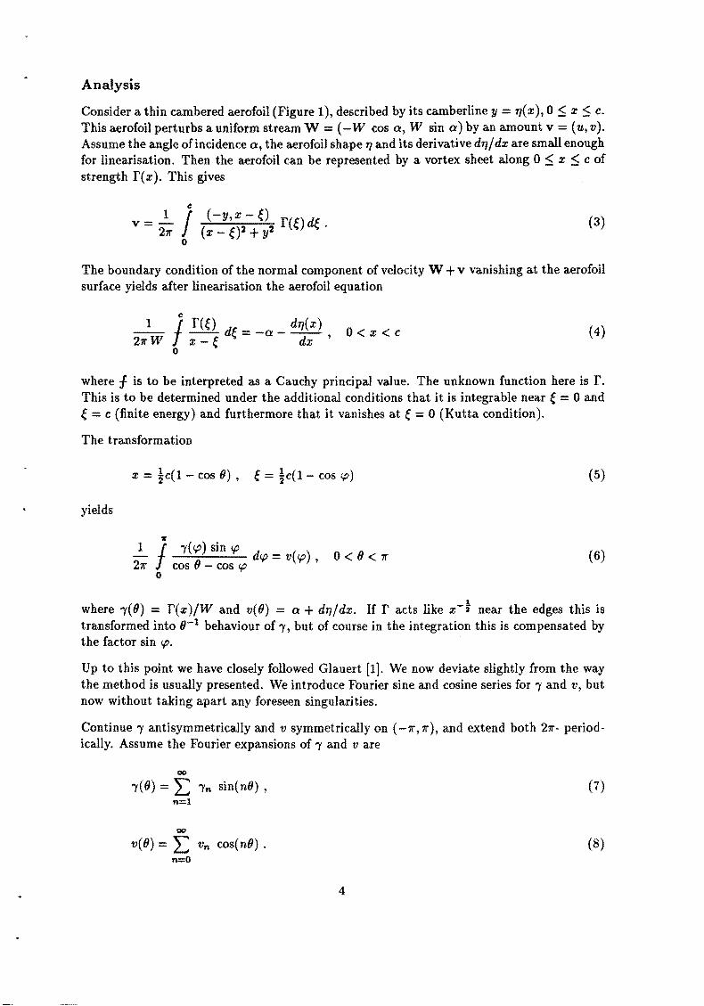
Analysis

Consider a thin cambered aerofoil (Figure 1 ), described by its camber line y = 17( x ), 0 ~ x :S c. This aerofoil perturbs a uniform stream W = (-W cos a, W sin a) by an amount v = ( u, v ). Assume the angle ofincidence a, the aerofoil shape 17 and its derivative d11/dx are small enough for linearisation. Then the aerofoil can be represented by a vortex sheet along 0 :S x 5 c of strength f(x). This gives

c - _!_ J (-y,x- {) f(t)dt

v- 211' (x-{)2+y2 ..... 0

(3)

The boundary condition of the normal component of velocity W + v vanishing at the aerofoil surface yields after linearisation the aerofoil equation

c

_1_ f f({) d{ =-a- dTJ(X) ' 0 <X< C 211' W X- { dx

0

(4)

where f is to be interpreted as a Cauchy principal value. The unknown function here is f. This is to be determined under the additional conditions that it is integrable near { = 0 and { = c (finite energy) and furthermore that it vanishes at { = o (Kutta condition).

The transformation

x = tc(l- cos 0) , { = tc(l- cos(;?) (5)

yields

'll'

1 j !((;?)sin t.p d ( ) - t.p=V(;?' 211' cos 0 - cos (;?

0

(6)

1 where 1(0) = f(x)/W and v(O) = a+ dTJ/dx. If r acts like x-i near the edges this is transformed into o-1 behaviour of 1, but of course in the integration this is compensated by the factor sin t.p.

Up to this point we have closely followed Glauert [1]. We now deviate slightly from the way the method is usually presented. We introduce Fourier sine and cosine series for 1 and v, but now without taking apart any foreseen singularities.

Continue 1 antisymmetrically and v symmetrically on ( -11', 11'), and extend both 211'- period­ically. Assume the Fourier expansions of 1 and v are

00

"Y( 9) = L In sin( n9) , (7) n=l

00

v(O) = L Vn cos(n9). (8) n=O

4

Of course, this continuation is only for convenience. It is possible to write any solution for which a Fourier series can be defined in this way. The sine series is certainly not chosen in order that the Kutta condition be fullfilled.

Substitution of (7) and (8) into (6), assuming that integration and summation may be ex· changed (which is consistent with the assumption of the existence of a Fourier series of 'Y), and then using (one of) the famous Glauert integrals ([1])

w w

f sin( n<p) sin <p d ( ()) f cos( n<p) d sin( nO) <p = -1!' cos n , <p = 1r ~~-'-cos <p - cos () cos <p - cos 0 sin 0

0 0

(9)

yields

co co

i L 'Yn cos( nO)= L Vn cos( nO), 0 < 6 < 1r. (10) n=1

Since in general v0 :f 0, equation (10) cannot be solved by any sequence ('Yn) in the ordinary sense. So it would seem that 'Y cannot be expanded into a Fourier series. As we will see, this is due to the non~integrable behaviour ,.... o-1 and ,.... (1r- e)-1 near the edges. So the transformation (5) together with the assumption of a Fourier series acts like a sieve allowing no solutions at alL The usual way to remedy this is to take the singularities apart (the tan( ie) in eq. {1)), however this is not necessary. A more direct way is to identify solutions with generalised functions ([32,33}), thus allowing a much wider class of Fourier series expansions.

The question now is how to make use of this greater freedom. We are free to add or subtract generalised functions provided we still satisfy equation (10). We then examine their effect on the Fourier series. Adding zero does not change anything since even in generalised sense the Fourier coefficients of the zero function are zero ([33], p.58). However, since equation (10) need only be satisfied on the open intervals 0 < (J mod 1r < 1r (i.e. excluding the end points), we may add generalised functions whose support is concentrated at the integer multiples of 1r

without affecting the general solution. Now, it is a standard theorem in generalised functions (Jones [32], p.89) that a generalised function has support concentrated at the origin only if it is a finite linear combintion of derivatives of delta functions. More explicitly,

if f(x) = 0 for x > 0 and x < 0

N

then f(x) = L anc<">(x) for any an and finite N. (11) n=O

This means that we can add multiples of the 211'·periodic 6-functions of 0 and ()- 1r, and its derivatives, to the righthandside of (10). Their generalised Fourier expansions ([32], p.153) are given by:

co co

211' L 6(1')( £J- 21rm) = L (in )Je einl (12) m=-co n=-oo

5

(similarly for 8 =: 8-1r). For the moment, however, we will restrict ourselves to the 6-function itself, since the derivatives lead to solutions too singular at the edges. So to equation (10) we add

00 co

21r L: 6(8- 27rm) = 1 + 2 L cos(n8) m=-oo n=l

A times, and

00 00

27r L: 6(8- 1r- 21r m) = 1 + 2 L ( -1)"' cos( nO) m=-co n=l

B times to obtain

co 00

! L "'n cos(n8) = Vo +A+ B + L (vn + 2A + 2( -1t B) cos(n8). n=l n=l

This equation has solution

B = -vo- A

"'n = 2vn - 4( -1 )"' Vo + 4( 1 - ( -1 t) A

Using the generalised identities ([32], p. 155)

00

I: sin(n8) = i cotan(!8) n=l

00

L (-1)"' sin(n8) = -! tan(l8) n=l

we obtain the usual form

co

'Y( 0) = 2vo tan( !8) + 2 L Vn sin( n8) + 4Af sin 0 . n=l

This is in physical coordinates

f(x)fW = ViTc co 2vo _ 1 / + 4ViTc Vl- x/c L Vn Un-t(l- 2xfc)

y 1- X C n.=l

1 +2A r:r: ,

yx,c vi- xfc

where Un denotes the Chebyshev polynomial of second kind and degree n, satisfying sin(n8) =sin 8 Un-1(cos 8) ([34]).

6

(13)

(14)

(15)

The factor of A in (15) is indeed the eigenfunction of the problem without Kutta condition (see [20]). For 17 (and so: v) smooth enough the Kutta condition is satisfied by taking A= 0.

Further generalisations

Motivated by the physics of the problem we have restricted ourselves until now to integrable singular behaviour of f. It is clear that once we have admitted generalised function solutions there is, other than physically, no restriction to the singular behaviour. We then have, in fact, an infinite number of eigensolutions. Although these eigensolutions may be of little importance practically, it is possible that they could play an unfavourable role in numerical solutions. We therefore include them here for the sake of completeness.

It is sufficient to consider equation (10) with zero right hand side. With equation {12) we then have in general

oo K oo

L i'n cosn9=Ao+Co+2 L L (-1)1cn21c[(A~c+(-1)"C~e) cos(nO) n=l k=O n=l

which has solutions

K

i'n = 2 L {-1)1cn21c(A~c + (-1)"C~c) (16) k=O

if

Clearly, the solution consists oflinear combinations of even derivatives of tan( jD) and co tan( !B). To see this, consider for k ~ 0

i'n = 2( -1 )" n2k '

then

d2k 00 d2k

7( B) = 2 dB2k L sin( nO) = d()2k cotan( lD) . n=l

(17)

Similarly, if

then

7

0,2/e CIO d2fc

1(8) = -2 d(J21e L ( -1)" sin( nO)= d(J21e tan(!O) . n=l

(18)

Conclusions

The classical series solution of the thin aerofoil problem developed by Glauert is cited through­out the literature. However, the role of the Kutta condition, together with the matter of uniqueness of the solution, sometimes seems to have escaped attention. It is either not men­tioned (since, in general, the Kutta condition is satisfied), or it is claimed to be satisfied by the pointwise behaviour of the chosen sine-series (which is not correct). This incorrect interpretation has not only relevance to the original incompressible 2 - D problem, but also to the application in more complex flow problems, to the finite wing problem where a very similar technique is used, and to numerical methods based on this type of series.

In the present note we have tried to rectify the incorrect interpretation that the choice of a Fourier-sine series is sufficient for the Kutta condition, and we have shown that in general the Kutta condition is only indirectly satisfied by excluding divergent series. By posing the problem in the context of generalised functions it is possible to handle divergent series, and the general, non-unique, solution can be found directly without further assumptions.

References

1. H. GLAUERT, The Elements of Aerofoil and Airscrew Theory, Cambridge University Press, Cambridge (1926) (p. 87).

2. G.K. BATCHELOR, An Introduction to Fluid Mechanics, Cambridge University Press, Cambridge (1967) (p. 467).

3. L.M. MILNE-THOMSON, Theoretical Aerodynamics, 2nd edition, MacMillan & Co, Lon­don (1952) (p. 138).

4. B. THWAITES (ed.), Incompressible Aerodynamics, Clarendon Press, Oxford (1960) (p. 123).

5. N.E. KocHIN, I.A. KIBEL' and N.V. RozE, Theoretical Hydrodynamics, Intersdence Publishers, New York (1964).

6. K. KARAMCHETI, Principles of Ideal-Fluid Aerodynamics, John Wiley & Sons, New York (1966) (p. 506).

7. H. ScHLICHTING and E. TR.UCKENBRODT, Aerodynamics of the Airplane, McGraw-Hill, New York (1979).

8. L.J. CLANCY, Aerodynamics, Pitman, London, (1975) (p. 172).

9. I.H. ABBOTT and A.E. VoN DOENHOFF, Theory of Wing Sections, Dover Publications, New York (1959) (p. 66).

8

10. A.M. KUETHE and C.~ Y. CHOW, Foundations of Aerodynamics, 4d ed., Wiley & Sons, New York (1986) (p. 116).

11. H.W. FoRSCHING, Grundlagen der Aeroelastik, Springer~ Verlag, Berlin (1974) (p. 255).

12. H. ASHLEY and M. LANDAHL, Aerodynamics of Wings and Bodies, Addison-Wesley, (1965) (p. 150).

13. N.A.V. PIERCY, Aerodynamics, 2nd ed., The English University Press, London (1947) (p. 241).

14. E.L. HoUGHTON and A.E. BROCK, Aerodynamics for Engineering Students, 2nd ed., Edward Arnold Publishers, London (1970) (p. 317).

15. B.K. SHIVAMOGGI, Theoretical Fluid Dynamics, Martinus NijhoffPublishers, Dordrecht (1985) (p. 139).

16. A.M. KUETHE and J.D. SCHETZER, Foundations of Aerodynamics, John Wiley, New York (1950) (p. 78).

17. W.J. DUNCAN, A.S. THOM and A.D. YouNG, The Mechanics of Fluids, Edw. Arnold, London (1960) (p. 589).

18. J.D. ANDERSON, Fundamentals of Aerodynamics, McGraw-Hill, London (1984) (p. 275).

19. J.H. SPURK, Stromungslehre, Springer-Verlag, Berlin (1987) (p. 350).

20. F.G. TRICOMI, Integral Equations, Interscience Publishers, New York (1957) (p. 173).

21. M.E. GOLDSTEIN, Aeroacoustics, McGraw-Hill, New York, (1976) (p. 230).

22. G.F. HOMICZ and J.A. LORDI, Three-dimensional theory for the steady loading on an annular blade row, AIAA Journal19 (4), (1981), 492-495.

23. S. KAJI and T. OKAZAKI, Generation of sound by rotor-stator interaction, Journal of Sound and Vibration 13 (3) (1970), 281-307.

24. N. NAMBA, Lifting surface theory for a rotating subsonic or transonic blade row, Aero­nautical Research Council Reports and Memoranda No. 3740 (1972).

25. N. N AM BA, Three-dimensional analysis of blade force and sound generation for an annular cascade in distorted flows, Journal of Sound and Vibration 50 (4) (1977), 479-508.

26. S.M. RAMACHANDRA, Acoustic pressures emanating from a turbo-machine stage, AIAA paper 84-2325 (9th Aeroacoustics Conference) (1984).

27. J.B.H.M. SCHULTEN, Sound generated by rotor wakes interacting with a leaned vane stator, AIAA Journal 20 (10) (1982), 1352-1358.

28. F. LANE and M. FRIEDMAN, Theoretical Investigations of Subsonic Oscillating Blade­Row Aerodynamics NACA TN 4136 (1958).

29. D.S. WHITEHEAD, Vibration and sound generation in a cascade of flat plates in subsonic flow, Aeronautical Research Council Reports and Memoranda No. 3685 (1972).

9

30. R.M. JAMES, On the remarkable accuracy of the vortex lattice method, Computer Methods in Applied Mechanics and Engineering 1 (1972), 59-79.

31. R. MITTRA and S. W. LEE, Analytical Techniques in the Theory of Guided Waves, The MacMillan Company, New York (1971).

32. D.S. JONES, The Theory of Generalised Functions, 2nd ed., Cambridge University Press, Cambridge (1982).

33. M.J. Lighthill, Introduction to Fourier Analysis and Generalised Functions, Cambridge University Press, Cambridge (1958).

34. M. ABRAMOWITZ and LA. STEGUN (ed.), Handbook of Mathematical Functions, Na~ tiona! Bureau of Standards (1964), (22.3.16).

10

' ' I I I

I y I I I I I I I I I I I I I

' I I

' ' I I I I I I I

Figure 1.

X

c

Camberline of thin aerofoil in stream W.