A nonlinear stability analysis of aircraft controller characteristics

outside the standard flight envelope

Stephen J. Gill, Mark H. Lowenberg and Simon A. NeildFaculty of Engineering, University of Bristol, Bristol, BS8 1TR, UK

Luis G. CrespoNational Institute of Aerospace, 100 Exploration Way,

Hampton VA 23666 USA

Bernd KrauskopfDepartment of Mathematics, University of Auckland,Private Bag 92019, Auckland 1142, New Zealand

Guilhem PuyouAirbus France, 31060 Toulouse Cedex 03, France

August 2014

Abstract

In this paper we evaluate the influence of the flight control system over the off-nominal flying dynamicsof a remotely operated air vehicle. Of particular interest is the departure/upset behaviour of the closed-loop system near stall. The study vehicle is the NASA Generic Transport Model and both fixed-gainand gain-scheduled versions of a LQR-PI controller are evaluated. The differences in effectiveness of thecontrollers are first demonstrated with time responses to fixed commands. Then, bifurcation analysis is usedto characterize spiral and spin behaviour of the aircraft in both open- and closed-loop configurations. Thisyields an understanding of the underlying vehicle dynamics outside the standard flight envelope, hence itprovides a means of assessing the effectiveness of the controller and evaluating the upset tendencies of theaircraft.

1 Introduction

The use of feedback control systems in civil aircraft is well established, with relatively complex control laws inplace on modern fly-by-wire airliners; see [1] for example. These are designed for nominal flight conditions wherethe aircraft is close to symmetric trimmed or manoeuvring flight, and incorporate envelope-limiting functionsto attempt to prevent excursions beyond the nominal flight envelope. The control law design process typicallyutilises linear methods, often based on linear time-invariant (LTI) models, even if the final controller is nonlinearby virtue of scheduling between gains designed at specific operating points.

Despite such control laws, that aim to maintain a safe operating envelope, the problem of airliners en-countering upset phenomena leading to loss-of-control (LOC) does exist [2]. This is characterised by a flighttrajectory involving large deviations in attitude and angular rates. During such excursions, the aircraft dynam-ics are dominated by aerodynamic forces and torques that are strongly nonlinear and might be coupled withthe moments of inertia and pilot commands. It is often of interest to determine if the flight controller plays abeneficial role on the recovery from vehicle upsets. Generally, LTI models are, however, of limited value whenanalysing nonlinear systems. Unfortunately, most of the mathematical tools for control analysis are based onsuch models [3].

1

A variety of control design approaches have been developed to overcome the limitations of linear controllers.A popular approach is gain-scheduling, where a set of linear controllers are designed at several operating pointsand then blended together with respect to an input or state variable [4]. They do, however, usually suffer thelimitation of being designed only at trim points within the expected operating envelope and, hence, may notcope well with nonlinearity under off-nominal conditions. Also, care needs to be exercised when scheduling withrespect to a state variable that changes rapidly. To overcome the limitations of linearity, much work has beendone on nonlinear control law design, such as by dynamic inversion [5] and a host of adaptive techniques [6, 7].These are also not necessarily problem-free, with issues such as robustness to model uncertainty and stabilityguarantees requiring special attention. Typically, nonlinear controllers are also evaluated only under nominaloperating conditions (i.e. those within the expected operating range, and up to the stall), partly because this ishow the design requirements are stipulated.

Whether implementing gain-scheduled control or another nonlinear approach, a suitably representative math-ematical model is needed. Due to the increased nonlinearity and time-dependence inherent in flight dynamicsbehaviour under off-nominal conditions – particularly at high angles of attack and/or sideslip – such models aremore difficult and expensive to create than conventional models and will inevitably incorporate far higher levelsof uncertainty. Hence, they do not generally exist for civil aircraft. However, researchers at NASA Langley havecreated the Generic Transport Model (GTM): this represents a dynamically scaled version of a twin-engine jetvehicle with a geometry characteristic of low-wing airliners with under-wing-mounted engines [8]. The purposeof the model, derived from a comprehensive wind tunnel test campaign as well as from remotely piloted tests ofa powered flight vehicle, was indeed to generate a representative wide-envelope airliner flight dynamics modelfor the simulation and analysis of upset and LOC [9]. A similar model was created for the EU ‘Simulation ofUPset Recovery in Aviation’ (SUPRA) research programme [10].

To gain insight into the behaviour of a nonlinear dynamical model, it is necessary to understand its ‘struc-ture’: its multiple steady state solution branches, their stability and changes thereof (at bifurcation points) andthe dependence of these structures on parameter variations. Whilst the generation of time history simulationsfrom such models is useful, it provides very limited information on the above. Numerical bifurcation analysis,on the other hand, implemented via continuation algorithms [11], has been shown to be extremely useful infacilitating an understanding of solution characteristics in state-parameter space, allowing response types to beinferred not only locally but also ‘globally’ across a wide operating region [12].

One field in which continuation and bifurcation analysis has indeed demonstrated significant value is thatof nonlinear flight dynamics of aircraft. Since the earliest applications, for example in Carroll and Mehra [13],Guicheteau [14] and Zagaynov and Goman [15], it has been applied to a number of military aircraft models,showing the development of phenomena such as wing rock, inertial coupling and spins (e.g. [16]) and the influenceof highly augmented control systems (e.g. [17]). Ref. [18] provides a comprehensive survey of bifurcation analysisapplied to fixed-wing flight dynamics problems. This approach has recently been implemented on the NASAGeneric Transport Model (GTM) [12] and the SUPRAmodel [10] in open-loop form, and has revealed spiral divesand steep spins. An early extension of the approach to closed-loop controllers deployed bifurcation analysis toassess the stability of a wing rock controller with different gains [19]. Bifurcation analysis of closed-loop aircrafthas primarily been used to analyse control laws; then the bifurcation diagrams were used to help design controlschemes to improve the aircraft behaviour. Littleboy and Smith [20] used bifurcation analysis to analyse open-loop and then closed-loop versions of the ‘Hypothetical High-Incidence Research Model’ to contribute to controllaw design through nonlinear dynamic inversion.

Jones et al. [21] developed the idea of dynamic gain-scheduling where the controller gains were designed asparameters varied within a continuation routine. Here, for each continuation step the trim point is calculatedand gains designed by means of a linear quadratic regulator (LQR). This defines a gain schedule with a superiorresolution, which is then transformed such that, when scheduled with a fast-varying state, the intended localstability remains valid. However, this method only concerns the aircraft in trim settings and does not assurethat off-nominal flight conditions have been stabilised. Bifurcation analysis of the NASA GTM aircraft coupledto a linear parameter varying (LPV) control system was performed by Kwatny et al. [22]. This used bifurcationanalysis to perform a rigorous examination of control and regulation around the stall point and showed howcontrollability is lost at bifurcation points; it also defined safe sets for the aircraft operation and consideredrecovery from upset in the presence of damage. However, whilst the dynamics of the closed-loop GTM aroundthe stall point was within the scope of this study, controller effects in other off-nominal conditions were not.

A note in [19] mentions how continuation methods can be used to help tuning the control law. This

2

idea is extended by Goman and Khramtsovsky [23] who also analysed a controller designed to suppress wingrock. Here, a two-parameter bifurcation diagram was used to show the combinations of gains for which thecontroller eliminated wing rock. However, these wing rock controllers use only simple proportional feedbackwhich, although successful for the suppression of wing rock, are not fully representative of controllers typicallyused on civil transport aircraft. Richardson et al. [24] extended this idea of continuing controller gains byuse of a scalar ‘gain parameter’ which is applied to the state-feedback gains in a feedback-plus-feedforwardgain-scheduled controller designed to meet handling qualities objectives by using eigenstructure assignment: iteffectively varies a selection of gains simultaneously between zero (when the gain parameter is zero) and theirdesign values (gain parameter unity) and beyond (gain parameter > 1). This study showed that, whilst desiredhandling qualities were achieved under nominal operating conditions, an undesirable isola that adversely affectssystem response was identified; it disappeared only when the gain parameter exceeded one. This illustrates thepower of numerical continuation when used to inform controller design. Although integral control was appliedto this system, the gain parameter continuation was applied only to the proportional gains, and was thereforerelatively simple in nature.

This paper extends the bifurcation analysis performed in [12] to analyse the dynamics of the GTM; it buildson the approach of Richardson et al. [24] to explore the means by which continuation methods can yield adeeper insight into the influence of control laws on the nonlinear system behaviour. Design of these controllaws is described in [25], and here analysis of both fixed gain and gain scheduled versions of the controlleris undertaken. The mathematical model of the closed-loop GTM consists of an airframe dynamics model –featuring aerodynamic, inertial, kinematic and control surface position and rate saturation nonlinearities –and a flight control system. The latter consists of (i) a longitudinal controller having the elevator deflectionsas control input, (ii) an auto-throttle having the throttle-input to both engines as control input, and (iii) alateral/directional multivariable controller having the ailerons and rudders as inputs. These controllers, whichassume a full-state feedback feedforward structure, define the control law. The feedforward component of thecontroller is driven by commands generated by the pilot. These commands, which are exogenous signals tothe system, are created by the pilot based on the aircraft’s current state and the desired steady-state flightcondition.

The paper is organized as follows. In Section II the aircraft model and controller architecture are describedand their performance briefly compared using time responses. In Section III the bifurcation analysis of the open-loop GTM is summarised, with an emphasis on upset behaviour; an assessment is then made of the changes inthe system attractors as the control loop is closed, focusing on the spiral and spin solutions and their respectivestability characteristics. Finally, in Section IV, conclusions are drawn concerning the changes in off-nominalattractors arising from using a control law, hence, the benefits offered by bifurcation methods in evaluatingclosed-loop flight dynamics.

2 Plant and Controller Architecture

2.1 The Generic Transport Model

The GTM is a model of a commercial transport aircraft for which both a dynamically scaled flight test vehicleand a high-fidelity simulation model were developed. Figure 1 shows the flight test vehicle and its conceptof operation. References [26, 8, 27] provide details on the vehicle’s configuration and characteristics and theflight experiments. The aircraft is piloted from a ground station via radio frequency links by using onboardcameras and synthetic vision technology. The high-fidelity simulation model, known as the DesignSim, usesnonlinear aerodynamic models extracted from wind tunnel data and system identification for conditions thatinclude high angles of attack, and considers actuator dynamics with rate and range limits, engine dynamics,sensor dynamics along with analog-digital-analog latencies and quantization, sensor noise and biases, telemetryuplink and downlink time delays, turbulence, atmospheric conditions, etc. The open-loop system model has 278state variables.

During stall, which occurs between angles of attack of 12◦ and 14◦ degrees, the vehicle experiences a dropin altitude and an uncommanded roll departure. These effects, which are captured by the aerodynamic modelof the DesignSim, mimic the behaviour of the test article observed in the flight experiments. A high leveldescription of the flight controllers used for in the bifurcation analysis is presented next. For additional detailson the development of these controllers, see [7].

3

Figure 1: NASA GTM test article and its concept of operations [7].

2.2 Control Design

The system dynamics can be represented as

X = F (X,U), (1)

where F is a nonlinear function of the state vector X and the control input U . For control design purposes,this nonlinear plant is linearized about a trim point (X∗, U∗) satisfying F (X∗, U∗) = 0 for the force andmoment equations. Deviations from the trim values X∗ and U∗ are written as lower-case letters hereafter, e.g.,X = X∗ + xp and U = U∗ + u. Linearization of Eq. (1) about the trim point leads to the system

xp = Apxp +Bpu+ ν(xp, u), (2)

where

Ap =∂F

∂X

∣∣∣∣X∗, U∗

Bp =∂F

∂U

∣∣∣∣X∗, U∗

(3)

and ν contains higher-order terms. In a sufficiently small neighbourhood of the trim point, the effect of thehigher-order terms is negligible. The LTI representation of the plant, which results from dropping the higher-order terms from Eq. (2), is given by

xp = Apxp +Bp(Rs(u) + d) +B2r, (4)

where Ap and Bp are the system and control input matrices, d(t) is an exogenous disturbance; r(t) is thereference command generated by the pilot; Rs(u) is a saturation function that enforces range saturation limitsin the control inputs, and B2 is the command input matrix.

The state, xp, consists of angle of attack, α; sideslip angle, β; speed, V ; roll rate, p; pitch rate, q; yaw rate,r; longitude, x; latitude, y; altitude, z; and the Euler angles, ψ, θ, and ϕ. The control input u consists of theelevator deflection, δe; the aileron deflection, δa; the rudder deflection, δr; and the throttle input to the engines,δth. The reference command r consists of angle of attack-, sideslip-, speed- and roll rate-commands. These fourcommands, denoted hereafter as αcmd, βcmd, Vcmd, and pcmd, respectively, are generated by the pilot to attainthe desired flight manoeuvre.

The flight controller consists of independent controllers for the longitudinal and the lateral/directional dy-namics. While the longitudinal controller consists of an auto-throttle and a multiple-input-single-output con-troller for pitch, the lateral/directional controller assumes a multiple-input-multiple-output structure. Thecontrollers operating the control surfaces have a linear quadratic regulator structure with proportional andintegral (LQR-PI) terms having integral error states for each of the components of the reference commandr. Furthermore, strategies for preventing integrator windup caused by input saturation were applied [7]. Afixed control allocation matrix that correlates inputs of the same class prescribes the 10 main plant inputs: 4elevators, 2 ailerons, 2 rudders and 2 throttles. As a result, out of these 10 inputs only 4 are independent.

4

2.2.1 Auto-throttle

The throttle input to the engines was prescribed by a simple proportional-derivative controller with the form

δth = K1eV +K2eV , (5)

where

eV = V − Vcmd. (6)

The regulation of airspeed and pitch control were done separately because of a large time scale separationbetween the corresponding actuators. In a previous work [7], a multivariable controller for both airspeed andpitch was developed.

2.2.2 Longitudinal Controller

The linearized plant for pitch control takes the form

xlon = Alonxlon +Blonulon, (7)

where Alon ∈ R3×3 is the system matrix, Blon ∈ R3×1 is the input matrix, xlon = [α q V ]⊤ is the state, andulon = δe is the input. To enable tracking commands in angle of attack, the integral error state

eα =

∫(α− αcmd)dt, (8)

was added. This led to the augmented plant[xloneα

]=

[Alon 0H1 0

] [xloneα

]+

[Blon

0

]δe +

[0−1

]αcmd, (9)

where H1 = [1, 0, 0]. A constant gain LQR controller that minimizes

J =

∫ ∞

0

(xTlonQxlon + δ2eR)dt, (10)

where Q = Q⊤ ≥ 0, R > 0 are weighting matrices, was designed. This led to

δe =[Klon Keα

] [xloneα

]. (11)

This controller must attain ample stability margins so the low-pass- and anti-aliasing-filters from sensors andthe delay caused by telemetry do not compromise stability.

The plant’s input is given by

Rs(u) =

u if umin < u < umax,

umax if u ≥ umax,

umin otherwise,

(12)

where u is the controller’s output, and umax and umin are the saturation limits of the actuator. The controldeficiency caused by this saturation function is given by

u∆ = Rs(u)− u. (13)

The integrator anti-windup strategy proposed in [7] is applied to the ⟨eα, δe⟩ pair.

5

2.2.3 Lateral/Directional Controller

An LTI model of the corresponding plant is

xlat = Alatxlat +Blatulat, (14)

where Alat ∈ R3×3 is the system matrix, Blat ∈ R3×2 is the input matrix, xlat = [β p r]⊤ is the state, andulat = [δa δr]

⊤ is the input. To enable satisfactory command following, integral error states for sideslip and rollrate, given by

eβ =

∫(β − βcmd)dt, (15)

ep =

∫(p− pcmd)dt, (16)

were added. The integral error in sideslip was chosen over that of the yaw rate to facilitate the generation ofcommands for coordinated turns with non-zero bank angles and cross-wind landing. The augmented plant isgiven by xlateβ

ep

=

[Alat 0H2 0

] xlateβep

+

[Blat

0

]ulat +

[0−I

] [βcmd

pcmd

], (17)

where H2 =[[1, 0]⊤ [0, 1]⊤ [0, 0]⊤

]. A LQR control structure for the lateral controller was adopted. This led to

[δaδr

]=

[Klat Keβ Kep

] xlateβep

. (18)

As before, this controller attains ample stability margins to accommodate for filters and time delays. Theanti-windup technique in [7] is applied to the ⟨eβ , δr⟩ and ⟨ep, δa⟩ pairs.

2.2.4 Control Allocation

Equations (5), (11) and (18) along with the three realizations of the anti-windup technique mentioned above,prescribe the preallocated input un = [δe δa δr δth]

⊤, where

un = Kn[xlon eα eV eV xlat eβ ep]⊤, (19)

and Kn ∈ R4×11 is the feedback gain. This input, along with a control allocation scheme, fully determines the10 control inputs of the aircraft. This relationship can be written as

unom = Gnomun, (20)

where Gnom ∈ R10×4 is the control allocation matrix. The allocation of un enforced by Gnom makes the fourelevators deflect the same, both ailerons deflect in opposite directions, the thrust of both engines equal, and thedeflection of both rudders equal.

2.3 Competing Control Alternatives

This section presents details of the development and configuration of the two flight control systems to beevaluated.

The open-loop longitudinal dynamics are unstable for angles of attack in the range 11.9◦-12.8◦ while thelateral/directional dynamics are unstable in the 10.4◦-14.25◦ and 23.85◦-28.4◦ ranges. Stall occurs in the firstof these three ranges. The non-zero aileron and rudder deflections necessary for trim are the result of minorasymmetries in the mounting of the engines, a slight offset between the centroid of the fuselage and the centre ofgravity (c.g.) and asymmetry in the vehicle aerodynamics. The asymmetry resulting from the engine mountingis more noticeable at high angles of attack because its effects are proportional to the engine’s thrust.

6

Figure 2: Aircraft states and commands corresponding to manoeuvres within the standard flight envelope forcontroller C1.

A single-trim-point flight controller for X∗ and U∗ was designed first, for a horizontal wings-level flightcondition and 80 knots (41.2m/s) air speed; the corresponding angle of attack is 4.28◦ and the flight path angle,γ, is zero. This controller consists of the auto-throttle, the longitudinal and the lateral/directional controllersintroduced above. This controller will be denoted as C1. The controller gains were tuned according to classicalcontrol metrics, which included stability margins, shaping of the input- and output-loop transfer-functions,and time responses to representative pilot commands. It is the fast modes of motion of the vehicle that areimportant in this process as the slower modes (in particular the spiral) can be compensated by either the pilotor an autopilot. The control objective was to obtain a controller that provides satisfactory pilot commandtracking given the intrinsic time delays of the system.

Figure 2 shows the states and commands corresponding to a typical manoeuvre within the normal flightenvelope. The aircraft starts off from the trim point used for control design and then it is subjected to commandsin angle of attack, side-slip, and roll rate. It can be seen that the controller tracked the doublets well whilereaching the commanded airspeed after a short transient without significant changes in altitude.

Figure 3 shows the same manoeuvre but for a sequence of commands centred about a trimmed point with ahigher angle of attack. A substantial degradation in tracking performance occurs because this flight conditionis far from the trim point X∗ used in the control design. Note that appearance of uncommanded oscillationsin pitch and the instabilities in both roll and yaw. Even though this controller attains good command trackingnear 4.28◦, it fails to locally stabilize the aircraft over the entire equilibrium manifold. Providing there isenough control authority, the aircraft might be kept near a locally unstable equilibrium point by a judiciousand persistent set of commands r.

To improve the command tracking performance outside the normal flight envelope, gain-scheduled controllerswere designed [28]. One of these, denoted as C2 and which can be regarded as moderately aggressive in itstracking performance, is considered in this paper. This controller schedules three fixed-point controllers on thelongitudinal and lateral axes with angle of attack. Since the scheduling variable is a state, the resulting controlleris quasi-linear parameter varying. The trim points used for control design correspond to angles of attack of4.28◦, 13◦, and 22◦. These values correspond to cruise, stall, and post-stall flight conditions, respectively. Eachof the fixed-point controllers comprising the gain scheduled controller attains good tracking performance near

7

Figure 3: Aircraft states and commands corresponding to manoeuvres outside the standard flight envelope forcontroller C1.

the corresponding linearization point. Furthermore, they make the important modes of the equilibrium manifoldlocally stable at each point in the 2◦-30◦ degree angle of attack range. The controller used by the gain scheduledcontroller at 4.28◦ is the very same C1.

In contrast to the fixed-point controller, C1, the gain-scheduled controller, C2, attains a command trackingperformance in all axes that is satisfactory and similar throughout the 2◦-28◦ degree range of angle of attack.For larger angles of attack, good V command tracking is no longer possible due to the reduced control authorityresulting from the saturation of the throttle input.

3 Bifurcation Analysis

In this section we first summarize aspects of the multi-attractor dynamics underlying the open-loop behaviourof the GTM, by means of bifurcation diagrams. We then consider how these change when the loop is closedwith the controllers C1 and C2, with particular emphasis on off-nominal conditions and upset with the controllerC1. Upset is defined in the Upset Recovery Training Aid (URTA) [29] as an inadvertent event where:

• Pitch angle, θ, goes beyond the set [−10◦, 25◦],

• Roll angle, ϕ, exceeds ±45◦,

• or flying with an inappropriate airspeed.

The other commonly used definition of upset is that by Lambregts et al. [30] where upset is an uncommandedor inadvertent event with an abnormal:

• attitude,

• rate of change of attitude,

• acceleration,

• airspeed, or

• with an inappropriate flight trajectory.

8

Table 1: Bifurcation diagram notation.

Stable equilibrium Hopf bifurcationStable 6-state equilibrium Torus bifurcationUnstable equilibrium Period doubling bifurcationStable periodic orbitUnstable periodic orbit

In this paper, these two often used definitions shall be used to assess which dynamics regimes uncovered by thebifurcation analysis represent upset conditions.

Results from numerical continuation applied to the GTM as described in Ref. [12] are presented here asone-parameter bifurcation diagrams; these indicate the dependence of steady state solutions of the dynamicalsystem on the variation of a single parameter. In the open-loop case, the parameter in the diagrams shown hereis elevator angle, whilst in the close-loop cases it is either the commanded angle of attack by the pilot αcmd ora ‘gain parameter’ GP on the controller gains (defined in Section 3.2). αcmd was chosen as the continuationparameter to allow comparison to the open-loop results. This is possible as the longitudinal controller turns anαcmd input into an elevator deflection, hence, there is a direct link between αcmd and δe in the closed-loop system.Local stability is indicated on the solution branches and is used, along with the topology of the diagrams andgeneral statements from bifurcation theory, to infer knowledge of the underlying global dynamics. The diagramsare generated with the method of numerical continuation, in this case using the software package AUTO [31]incorporated into the Matlab Dynamical Systems Toolbox [32]. The line types and symbols adopted here todefine whether solutions are equilibria or limit cycles, stable or unstable, and to denote bifurcation points arelisted in Table 1.

Note that a one-parameter bifurcation diagram for an nth-order system occupies (n+1)-dimensional space;bifurcation diagrams are shown as 2D projections of this space, i.e. one state versus the chosen continuationparameter. Selected projections are shown, aimed at revealing the main features of the behaviour.

3.1 Open-loop characteristics

The open-loop system is 8th-order, with state vector [α β V p q r θ ϕ]. This omits the ψ and ground-positionstates of the system described in equation (4) since these play a negligible role in the flight dynamics behaviourof the aircraft. Figure 4 shows the α and p projections of the open-loop system bifurcation diagram for theGTM. The starting solution was a trim point at a prescribed altitude and angle of attack: 800 ft (243m) andα = 3◦; the associated forward speed is V = 47.3m/s. The corresponding parameter values are: throttle 22.1%,elevator deflection δe = 2.58◦ and aileron and rudder close to zero (−0.004◦ and 0.009◦ respectively). In additionto the small thrust asymmetry in the model, the aerodynamics is not symmetric about the x-z plane for zeroaileron and rudder. The asymmetry is, however, very small at low angles of attack. Aileron, rudder and throttleremain fixed at these values, whilst δe is the continuation parameter.

The behaviour shown in Fig. 4 is described in detail in Ref. [12]. The salient types of behaviour are labelledA–G and summarised in Table 2.

Table 2: Summary of characteristics of GTM open-loop behaviour in Fig. 4 (from [12]).

Symbol Type of Dynamics α rangeA Stable trimmed symmetric flight −2◦ to 8◦

B Low frequency oscillations 2.2◦ to 21◦

C Steady steep spiral 10.5◦ to 20.9◦

D Inverted spiral −5◦ to −2◦

E Steady steep spin 30.5◦ to 38.8◦

F Period-one oscillatory steep spin 32.7◦ to 38.5◦

G Period-three oscillatory steep spin 30.8◦ to 40◦

9

−30 −20 −10 0 10 20−5

0

5

10

15

20

25

30

35

40

45

−30 −20 −10 0 10 20−250

−200

−150

−100

−50

0

50

100

150

200

250α[deg]

δe [deg]

A

B

C

D

E F

G

p[deg/s]

δe [deg]

A

BC

C

D

E

F G

(a) (b)

Figure 4: Open-loop bifurcation diagram in angle of attack (a) and roll rate (b), from [12].

Of specific interest in terms of upset are the steady steep spirals C, the steady spin E and the two oscillatoryspins F and G. The steep spirals of regime C exist for both positive and negative p and form descending spiralsto the right and left respectively. Angular rates are reasonably large with p exceeding 60◦/s and along withthis, ϕ ≈ ±60◦ and flight path angle, γ, reaches −70◦. For these reasons, regime C can be classified as an upsetcondition, within the requirements designated by both the URTA [29] and Lambregts et al [30]. The steadyspin of regime E was found to exist only for positive p and is characterised by large angular rates and γ ≈ −89◦,indicating that, in this regime, the GTM would be falling near to vertical. However, it was found that, althoughthis dynamic regime is also a serious upset condition, it is a weak attractor and time history simulations wereunable to access the branch without being exactly initialised on it; they were attracted to the steep spiral ofregime C.

The two oscillatory spins, however, represent much stronger attractors in the open-loop GTM. These alsoexhibit large angular rates and large negative γ but were found to be accessible for the GTM by the use oflarge rudder inputs at high pitch up elevator [12]. Regime F is a period-one periodic orbit with a time periodof ≈ 1s while regime G is a period-three periodic orbit with a time period of ≈ 3s. The small time period ofthese oscillations, along with the angular rates and γ, infer that these periodic orbits can be classed as upset bythe criteria described and, in fact, represent the most severe form of upset exhibited by the open-loop GTM.

3.2 Closed-loop characteristics

3.2.1 αcmd bifurcation diagrams – controller C1The controller C1 was designed for a single trim condition at α = 4.28◦ and V = 41.2m/s whilst for C2 aseries of such γ = 0 trims were used. This condition yields an implicit dependency between αcmd and Vcmd.This dependency is replicated in the generation of bifurcation diagrams for the closed-loop system: the sametrim function as that adopted in the controller design was used to define a schedule of Vcmd inputs versuscontinuation parameter αcmd; this schedule was then implemented during the numerical continuation runs suchthat Vcmd and, hence, throttle setting, also change as αcmd varies. This means that the branch of trim solutionson the bifurcation diagrams corresponds directly with the conditions previously used to assess the controllersand ensures symmetric trim solutions with γ = 0◦.

In this analysis, a reduced-order model of the GTM was used to characterize the stability of the system inorder to relate results to that used in the control law design process. This incorporated the fast-varying states[α β V p q r ]; the slow varying modes (spiral and phugoid) are ignored in this analysis because their instabilitycan be easily controlled by either the pilot via reference commands, or an autopilot. The bifurcation analysis,

10

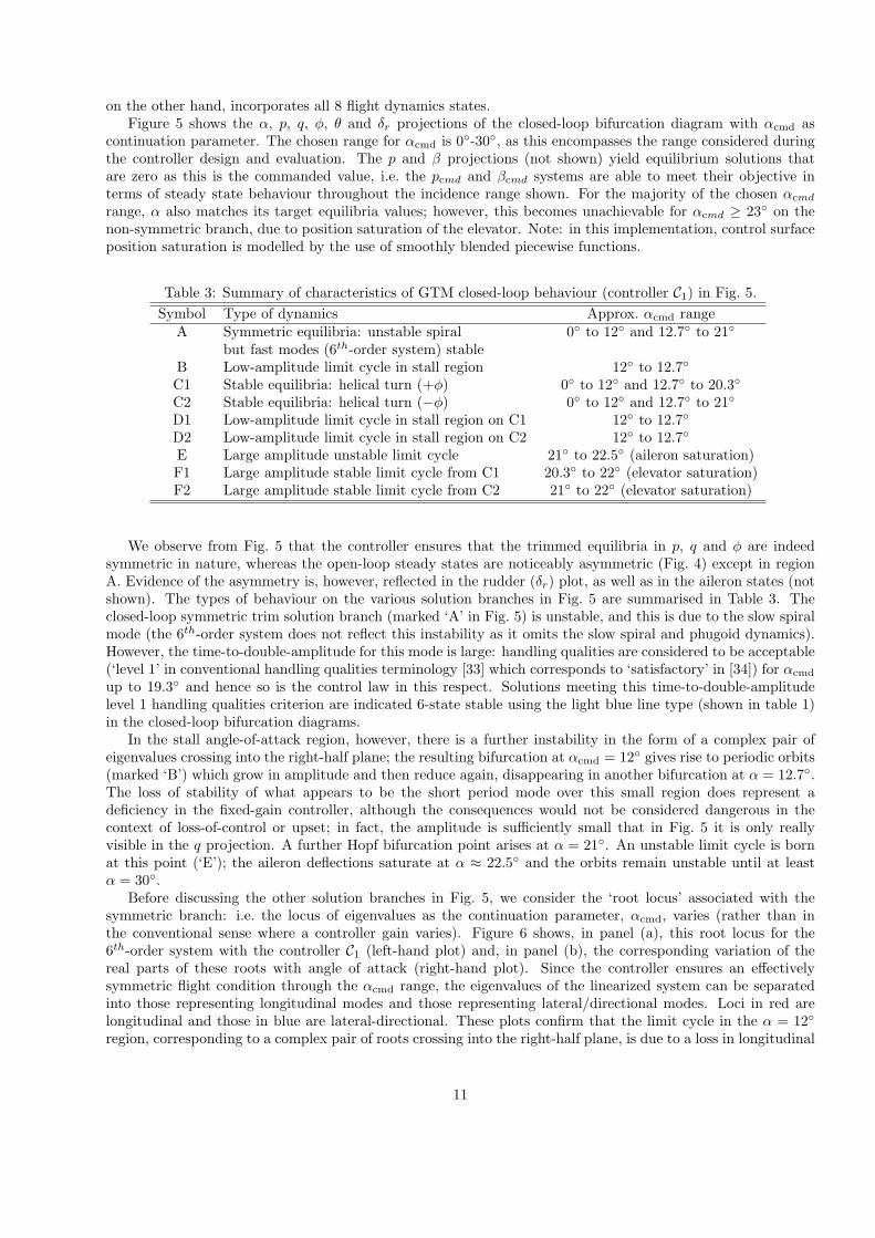
on the other hand, incorporates all 8 flight dynamics states.Figure 5 shows the α, p, q, ϕ, θ and δr projections of the closed-loop bifurcation diagram with αcmd as

continuation parameter. The chosen range for αcmd is 0◦-30◦, as this encompasses the range considered duringthe controller design and evaluation. The p and β projections (not shown) yield equilibrium solutions thatare zero as this is the commanded value, i.e. the pcmd and βcmd systems are able to meet their objective interms of steady state behaviour throughout the incidence range shown. For the majority of the chosen αcmd

range, α also matches its target equilibria values; however, this becomes unachievable for αcmd ≥ 23◦ on thenon-symmetric branch, due to position saturation of the elevator. Note: in this implementation, control surfaceposition saturation is modelled by the use of smoothly blended piecewise functions.

Table 3: Summary of characteristics of GTM closed-loop behaviour (controller C1) in Fig. 5.

Symbol Type of dynamics Approx. αcmd rangeA Symmetric equilibria: unstable spiral 0◦ to 12◦ and 12.7◦ to 21◦

but fast modes (6th-order system) stableB Low-amplitude limit cycle in stall region 12◦ to 12.7◦

C1 Stable equilibria: helical turn (+ϕ) 0◦ to 12◦ and 12.7◦ to 20.3◦

C2 Stable equilibria: helical turn (−ϕ) 0◦ to 12◦ and 12.7◦ to 21◦

D1 Low-amplitude limit cycle in stall region on C1 12◦ to 12.7◦

D2 Low-amplitude limit cycle in stall region on C2 12◦ to 12.7◦

E Large amplitude unstable limit cycle 21◦ to 22.5◦ (aileron saturation)F1 Large amplitude stable limit cycle from C1 20.3◦ to 22◦ (elevator saturation)F2 Large amplitude stable limit cycle from C2 21◦ to 22◦ (elevator saturation)

We observe from Fig. 5 that the controller ensures that the trimmed equilibria in p, q and ϕ are indeedsymmetric in nature, whereas the open-loop steady states are noticeably asymmetric (Fig. 4) except in regionA. Evidence of the asymmetry is, however, reflected in the rudder (δr) plot, as well as in the aileron states (notshown). The types of behaviour on the various solution branches in Fig. 5 are summarised in Table 3. Theclosed-loop symmetric trim solution branch (marked ‘A’ in Fig. 5) is unstable, and this is due to the slow spiralmode (the 6th-order system does not reflect this instability as it omits the slow spiral and phugoid dynamics).However, the time-to-double-amplitude for this mode is large: handling qualities are considered to be acceptable(‘level 1’ in conventional handling qualities terminology [33] which corresponds to ‘satisfactory’ in [34]) for αcmd

up to 19.3◦ and hence so is the control law in this respect. Solutions meeting this time-to-double-amplitudelevel 1 handling qualities criterion are indicated 6-state stable using the light blue line type (shown in table 1)in the closed-loop bifurcation diagrams.

In the stall angle-of-attack region, however, there is a further instability in the form of a complex pair ofeigenvalues crossing into the right-half plane; the resulting bifurcation at αcmd = 12◦ gives rise to periodic orbits(marked ‘B’) which grow in amplitude and then reduce again, disappearing in another bifurcation at α = 12.7◦.The loss of stability of what appears to be the short period mode over this small region does represent adeficiency in the fixed-gain controller, although the consequences would not be considered dangerous in thecontext of loss-of-control or upset; in fact, the amplitude is sufficiently small that in Fig. 5 it is only reallyvisible in the q projection. A further Hopf bifurcation point arises at α = 21◦. An unstable limit cycle is bornat this point (‘E’); the aileron deflections saturate at α ≈ 22.5◦ and the orbits remain unstable until at leastα = 30◦.

Before discussing the other solution branches in Fig. 5, we consider the ‘root locus’ associated with thesymmetric branch: i.e. the locus of eigenvalues as the continuation parameter, αcmd, varies (rather than inthe conventional sense where a controller gain varies). Figure 6 shows, in panel (a), this root locus for the6th-order system with the controller C1 (left-hand plot) and, in panel (b), the corresponding variation of thereal parts of these roots with angle of attack (right-hand plot). Since the controller ensures an effectivelysymmetric flight condition through the αcmd range, the eigenvalues of the linearized system can be separatedinto those representing longitudinal modes and those representing lateral/directional modes. Loci in red arelongitudinal and those in blue are lateral-directional. These plots confirm that the limit cycle in the α = 12◦

region, corresponding to a complex pair of roots crossing into the right-half plane, is due to a loss in longitudinal

11

0 5 10 15 20 25 300

5

10

15

20

25

30

0 5 10 15 20 25 30−15

−10

−5

0

5

10

15

20

25

30

35

0 5 10 15 20 25 30−15

−10

−5

0

5

10

15

20

25

30

0 5 10 15 20 25 30−50

−40

−30

−20

−10

0

10

20

30

40

50

0 5 10 15 20 25 30−60

−40

−20

0

20

40

60

0 5 10 15 20 25 30−8

−6

−4

−2

0

2

4

6

8

α[deg]

αcmd [deg]

A, C1, C2

B, D1, D2

EF1

F2

p[deg/s]

αcmd [deg]

A, C1, C2 B, D1, D2E

F1

F2

q[deg/s]

αcmd [deg]

AB

C1, C2 D1, D2

E

F1

F2

φ[deg]

αcmd [deg]αcmd [deg]

AB

C1

C2

D1

D2

E

F1

F2

θ[deg]

αcmd [deg]

A

B

C1, C2

D1, D2

E

F1

F2

δ r[deg]

αcmd [deg]

ABC2

C1

D2

D1

E

F2

F1

(a) (b)

(c) (d)

(e) (f)

Figure 5: Closed-loop bifurcation diagram, for controller C1: panels (a)-(f) show α, p, q, ϕ, θ and δr projections,respectively.

12

−14 −12 −10 −8 −6 −4 −2 0 2−10

−8

−6

−4

−2

0

2

4

6

8

10

−4 −3 −2 −1 0 1 20

5

10

15

20

25

30Imaginarycomponent

Real component

αcmd[deg]

Real component

(a) (b)

Figure 6: Closed-loop root locus for the 6th-order system (a), and corresponding variation of real parts withangle of attack (b), for symmetric solution branch and controller C1. Red loci are longitudinal roots and bluelateral-directional.

stability. We also see that a lateral-directional root enters the right-half plane at α = 21◦, causing the Hopfbifurcation in Fig. 5.

In addition to the symmetric solution branch discussed above, we note in Fig. 5 that there are two branchesof stable equilibria arising at zero angle of attack (denoted ‘C1’ and ‘C2’). These are close to anti-symmetricin the lateral-directional sense (i.e. the value of β, p, r or ϕ at a particular αcmd on C1 is virtually equal inmagnitude and is of opposite sign to that on branch C2, whilst the longitudinal variables are equal in valueand sign on C1 and C2). Close inspection of these solutions shows that they represent helical trajectories –descending turns – with pitch angle θ = 0◦. This is due to the kinematics of an aircraft constrained in aturn with zero roll rate, due to the pcmd = 0 function in the controller. In particular, consideration of the ϕand θ kinematic equations under equilibrium conditions with p = 0 reveals that r tan θ must be zero. For thesymmetric solution branch, denoted A in Fig. 5, yaw rate is zero so that r tan θ will be zero whatever the valueof θ; however, for the turning solution where r = 0, pitch angle θ must be zero for the kinematic constraint tobe met. By definition γ = θ − α so that the helical turn solutions in the bifurcation diagram, where αcmd ≥ 0,require γ to be negative – denoting descending flight.

It is worth comparing the ‘off-nominal’ behaviour of the closed-loop aircraft helical turn solutions withthose of the open-loop steep spirals indicated as regions C in Fig. 4. The flight path angle for the closed-loopdescending turns is substantially lower than that of the open-loop steep spiral, where γ reaches −70◦. Also,the groundtrack radius, calculated by simulation of the full nonlinear 12th-order system, is far tighter for theopen-loop spiral; in fact, an order of magnitude smaller than the helical turn radii. Comparing the behaviourof the helical turns with that considered upset the only condition exceeded is that ϕ ≥ ±45◦ and even then thisis just for the portion of the branches between 7◦ < αcmd < 11◦. Thus the stable portions of the descendingturn solution branches do not reflect upset conditions for the majority of the αcmd range, unlike the open-loopsteep spiral, showing improved upset behaviour with the addition of controller C1.

As with the symmetric branch, the turning solutions also lose stability in the α = 12◦-12.7◦ range associatedwith wing stall for this small-scale airliner configuration. Again, the amplitudes of the resulting limit cycles(D1 and D2) are small and only really visible in the projections of q in Fig. 5(c). Furthermore, there areadditional Hopf bifurcation points on these branches in the region of 20◦-21◦ incidence – again mirroring theloss of stability at a similar incidence on the symmetric branch. These are supercritical Hopf points, where theperiodic orbits (F1 and F2) that grow from them are stable; they increase in amplitude as αcmd increases untilthe elevator and ailerons saturate during parts of the orbits (as from αcmd ≈ 22◦) and maintain stability untilat least αcmd = 30◦. This mirrors periodic orbit E from the symmetric branch. The very slight asymmetry

13

0 5 10 15 2018

22

26

0 5 10 15 200

25

50

0 5 10 15 20−50

0

50

0 5 10 15 20−20

−10

0

10

α[deg]

t [s]

φ[deg]

t [s]

p[deg/s]

t [s]

θ[deg]

t [s]

(a)

(b)

(c)

(d)

Figure 7: Closed-loop time history with αcmd fixed at 23◦ on the oscillatory turn for controller C1. Panels(a)-(d) show α, p, ϕ and θ responses, respectively.

present in the system on these anti-symmetric branches is not easy to observe in Fig. 5, although the differencein αcmd values at which the F1 and F2 limit cycles occur on each of the two branches is visible.

The time history of periodic orbit F1 with αcmd fixed at 23◦ shown in Fig. 7 implies that this periodicorbit is a much more dangerous flight condition than those on the stable parts of the C1 helical turn branch.Although altitude is lost more slowly during this oscillating turn than in the open-loop steep spiral and steepspin solutions, the rapid large magnitude roll excursions could induce excessive loads on the aircraft. Hence,even though the flight parameters lie within that often considered upset by the URTA, periodic orbits F1 andF2 can be considered as potential upset solutions due to the large rate of change of attitude. However, thebifurcation diagrams indicate that recovery away from these attractors can be simply attained by reducing αcmd

to below the value at which the Hopf bifurcations occur; this will return the aircraft to a stable descendingturning solution.

3.2.2 αcmd bifurcation diagrams – controller C2As described in Section 2.3, controller C2 is gain scheduled based on three trim points at angles of attackcorresponding to cruise, stall and post-stall flight conditions (4.28◦, 13◦ and 22◦, respectively). Given thebifurcation diagrams shown thus far, these design points are seen to be well suited to accommodate the nonlinearnature of the GTM dynamics and so we would expect a well-designed gain scheduled controller to stabilize thesolutions through the limit cycle regions described above for the fixed-gain controller (i.e., referring to Fig.5/Table 3, around points B, D1 and D2 in the 12◦-13◦ angle of attack region and points E, F1 and F2 above20◦ angle of attack).

Figure 8 shows the α, p, q and ϕ projections of the bifurcation diagram for controller C2; it was generatedas that for controller C1 shown in Fig. 5, i.e. again using αcmd as the continuation parameter and with the sameVcmd schedule to maintain γ = 0 on the symmetric branch.

By evaluating the time-to-double-amplitude, the unstable spiral mode on the symmetric branch now satisfies,for C2, the level 1 handling quality criterion up to a slightly higher angle of attack (αcmd = 21.5◦) than thatfor the fixed-gain controller C1. More importantly, it is evident from the bifurcation diagram in Fig. 8 that thegain-scheduled controller C2 stabilises all the periodic orbits that were exhibited on both the symmetric and thehelical turn solution branches in the case of controller C1. This implies that C2 stabilises the aircraft throughoutthe useable αcmd range.

3.3 Application of the gain parameter to all controller gains

The principal interest in using bifurcation methods to assess the impact of control laws is to investigate off-nominal conditions and, in particular, the influence of attractors associated with unwanted behaviour – includingupset. The open-loop GTM is prone to entering the steep spiral region (C in Fig. 4), which can be considereda form of upset behaviour; it can also enter the oscillatory spin regions (F and G in Fig. 4) which are, of

14

0 5 10 15 20 25 300

5

10

15

20

25

30

0 5 10 15 20 25 30−5

0

5

10

15

20

0 5 10 15 20 25 30−5

−4

−3

−2

−1

0

1

2

3

4

5

0 5 10 15 20 25 30−60

−40

−20

0

20

40

60

α[deg]

αcmd [deg]

A, C1, C2

p[deg/s]

αcmd [deg]

A, C1, C2

q[deg/s]

αcmd [deg]

A

C1, C2

φ[deg]

αcmd [deg]

A

C1

C2

(a) (b)

(c) (d)

Figure 8: Closed-loop bifurcation diagram, controller C2: panels (a)-(d) show α, p, q and ϕ projections, respec-tively.

course, particularly dangerous (although recoverable). A flight controller has the potential of modifying such abehaviour but might not be able to fully eradicate it: the solution branches representing undesirable behaviourmay move in state-parameter space but could potentially still play a role in inducing upset conditions when,for example, the aircraft is subject to a large disturbance. In order to investigate these effects, we carry outnumerical continuation with a ‘gain parameter’, GP, as the continuation parameter to represent the transitionfrom open- to closed-loop. This so-called ‘homotopy’ parameter is simply a factor applied to one or more of thecontroller gains, such that when GP=0 the gains are zero (open loop) and when GP=1 the relevant gains areat their design values for the controller under consideration. It can also be increased beyond 1 to explore thestability margins of the controller. This analysis enables determining a range of controller gains for which thecontroller is effective.

Figure 9 shows this open-to-closed-loop transition when continuation parameter GP is applied to all thegains, i.e. those on the command paths and those on the stability augmentation paths. The continuation wasinitiated at the point GP=1 and then the controller gains were varied away from the design point in bothnegative and positive directions to investigate the performance of controllers that are less and more aggressiverelative to the baseline controller respectively. To carry out this analysis, consideration must be given to the

15

0 0.5 1 1.5 216

16.5

17

17.5

18

18.5

19

19.5

20

20.5

21

0 0.5 1 1.5 2−60

−40

−20

0

20

40

60

0 0.5 1 1.5 2−60

−40

−20

0

20

40

60

0 0.5 1 1.5 2−5

−4

−3

−2

−1

0

1

2

3

4

5

α[deg]

GP

A, C1, C2

p[deg/s]

GP

A, C1, C2

φ[deg]

GP

A

C1

C2

δ r[deg]

GP

A

C2

C1

(a) (b)

(c) (d)

Figure 9: Closed-loop bifurcation diagram, for controller C1: panels (a)-(d) show α, p, ϕ and δr projections,respectively. Continuation is with respect to the gain parameter, GP.

constant values used for the controller commands since the GP=0 and GP=1 points may be very differentflight conditions, especially at GP=0 which is equivalent to open-loop flight. In this case, controller commandscorresponding to symmetric trim at αcmd = 20◦ were chosen, because this was close to the point of lateral-directional instability that manifests itself in periodic orbits E, F1 and F2 in Fig. 5. As the gain parameter isvaried, the controller commands remained fixed at their γ = 0 trim settings for α = 20◦, namely αcmd = 20◦,Vcmd = 49m/s and pcmd = βcmd = 0. This gives rise to an ‘instantaneous’ demand on the controlled variablesas soon as GP increases above zero, which is particularly evident in p and β as their commanded values are farfrom those in open-loop.

It is evident from Fig. 9 that, when the controller is operative (GP¿0), it attempts to drive the states to thepilot commands, even when the gain is very small. This results in a very dramatic change in the equilibriumsolutions as the gain increases slightly from zero. The jump in α is only present in the two equilibrium brancheswhere ϕ = 0 and not for the symmetric branch. This is the case because the controller is trimmed for thesymmetric branch at α = 20◦: the elevator deflection for this condition is δe = −11.95◦ but whilst for open-loopthis elevator deflection ensures that α = 20◦, for the steep spiral – the non-symmetric branches in Fig. 9 –an elevator deflection of δe = −11.95◦ gives α ≈ 16◦. The jump arises from the αcmd path of the control law

16

and decreases δe until α = 20◦ is achieved. Note that, while the controller is able to significantly alter theequilibria for even a very small gain, any transient dynamics here are likely to be rather slow. As the controlleris ‘turned on’, the state variables move to the commanded values, even if the control gains are tiny; the otheruncommanded states vary as GP varies and reach the full closed-loop values when GP=1. However, at smallgains (where GP≤ 0.25), stability is lost on all three branches at Hopf bifurcations.

This form of continuation run reveals the potential for the continuation and bifurcation analysis techniqueto provide insight into the impact of controller changes, both near and away from nominal design conditions.In the case considered here, the controller gains must be greater than a quarter of the nominal value in order toachieve stability. Figure 9 also indicates that to achieve level 1 spiral mode handling qualities on the symmetricbranch for C1 at α = 20◦, the parameter GP needs to be in excess of about 1.45 (cf. Fig. 5 where the spiralmode rate of divergence no longer meets level 1 handling quality levels once αcmd exceeds 19.3◦).

Other smoothly-varying controller characteristics could also be evaluated in the same way, allowing insightinto closed-loop behaviour in regions away from the baseline controller; such characteristics may not be identifiedwhen only conventional linear methods are deployed. The gain parameter bifurcation diagram for the controllerC2 in Fig. 10 shows similar behaviour. Due to the gain-scheduling, the nominal value of the gains of this controllerare larger than those of C1 at αcmd = 20◦ and, hence, the system loses stability on the descending turn branchesonly once GP is reduced below about 0.15. Also, for the symmetric branch, controller C2 maintains level 1handling qualities for GP values down to approximately 0.5 which represents superior performance over C1.

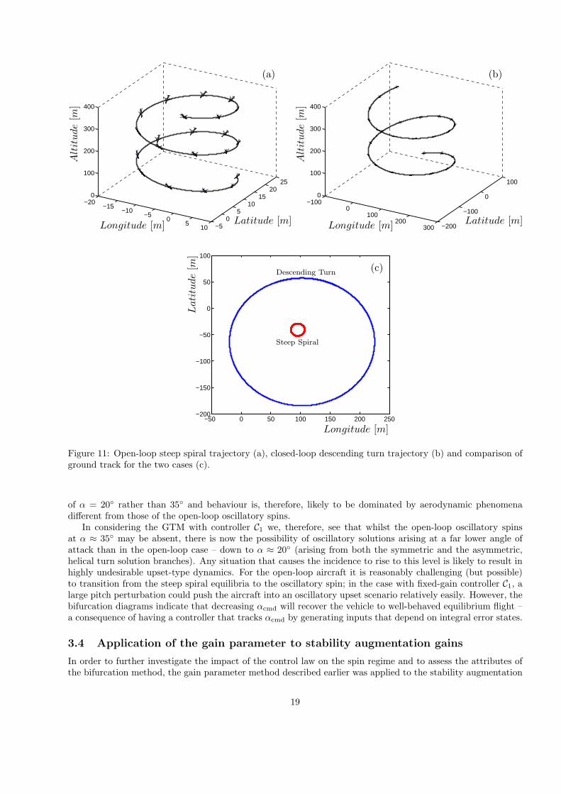
From Figs. 9 and 10 it is clear that, as soon as the controller is activated, the open-loop steep spiralsolution is ‘converted’ into the helical turn solution. In addition to all the commanded states switching to theircommand values, θ → 0 as p→ 0 due to the kinematic effect described above. This descending turn behaviouris acceptable and certainly preferable from a safety perspective to the dangerous open-loop steep spiral. Figure11 compares the open-loop spiral and the closed-loop descending turn solutions by depicting their trajectories.This confirms that, while the open-loop spiral is a rapid rotation with small radius, the closed-loop response isfar slower (a full turn takes approximately five times longer than in the spiral) and with a substantially largerradius.

Figure 5 revealed that the helical turn equilibria lose stability at α ≈ 21◦ − 22◦ for controller C1. The choiceof αcmd = 20◦ for generating the gain parameter bifurcation diagram of Fig. 9 means that the system steadystates are close to becoming unstable. Indeed, we observe that, if GP is increased just beyond a value of 1, theC1 (positive ϕ) turning solution in Fig. 9 loses stability at a Hopf bifurcation. This indicates that, at this point,controller C1 has limited stability margin. The branch C2 (negative ϕ) does not lose stability until GP ≥ 1.55,which shows that the descending turn with negative ϕ is a more robust solution than that for positive ϕ. Thisdifference is likely due to the asymmetry of the physical GTM aircraft mentioned in section 3.1 rather than thecontroller. The loss of stability of C1 so close to the nominal controller gains would not be expected – althoughit is clear that the controller C1 is operating far away from the design point of α = 4.28◦. This potential lackof robustness is not seen in the bifurcation diagrams for controller C2 in Fig. 10, which has a gain-schedulingdesign point at α = 22◦. The dependence of such features on parameter variations is clearly portrayed via thebifurcation diagrams and these suggest that the gain-scheduling of controller C2 is significantly more robustthan C1 at high angles of attack.

The structure of the control law (integral control over integral error states) is such that the steady statesolutions adopt the commanded values even for extremely small gain parameter. This is ‘just beyond’ open-loopand is due to the integral terms on the command path which will increase in magnitude until the commandvalues or the control surface limits are reached. Provided that there is sufficient control power, the integratorwill always reach the commanded values in the steady state. However, in practice the transient response wouldbe slow if the gains were small because the integrators would take considerable time to respond to the commands(even if the equilibrium was stable). In the example for C1 shown in Fig. 9 the helical turn equilibria are allunstable for GP ≤ 0.25. The periodic solutions which would arise from the Hopf bifurcations have not beenconsidered here, as the primary interest for the design of controller gains is the point where the controllers losestability rather than the behaviour past this point.

Figure 12 shows the responses in α for a number of time histories, each for controller C1, with differentvalues of GP corresponding to Fig. 9 – ranging from 0.01 to 1. In each case, the simulation starts with GP=0(open loop) and the GP value ramps up linearly to the new non-zero value over the time interval from 50 to51 seconds. The responses for GP=0.01 and GP=0.1 exhibit the expected unstable behaviour for controllerC1 at low gain parameter. At GP=0.1 the solution is periodic but for GP=0.01, the solution is more complex

17

0 0.5 1 1.5 215

16

17

18

19

20

21

0 0.5 1 1.5 2−60

−40

−20

0

20

40

60

0 0.5 1 1.5 2−60

−40

−20

0

20

40

60

0 0.5 1 1.5 2−2

−1.5

−1

−0.5

0

0.5

1

1.5

2

α[deg]

GP

A, C1, C2

p[deg/s]

GP

A, C1, C2

φ[deg]

GP

A

C1

C2

δ r[deg]

GP

A

C2

C1

(a) (b)

(c) (d)

Figure 10: Closed-loop bifurcation diagram, for controller C2: panels (a)-(d) show α, p, ϕ and δr projections,respectively. Continuation is with respect to the gain parameter, GP.

and the amplitude varies significantly. For values of GP higher than 0.25, we expect a stable response. This isevident for GP=0.3, 0.5 and 0.8 but when GP=1 a periodic orbit is induced. This is, at first glance, unexpectedas the equilibria are stable for GP=1, and it implies that controller C1 is particularly bad at dealing with thisupset condition. As noted, the bifurcation diagrams in Fig. 5 show that the αcmd = 20◦ solution is very near aHopf bifurcation, which explains why in the presence of a disturbance the response appears to be approachinga limit cycle rather than an equilibrium solution. This suggests that the Hopf bifurcation in the gain parameterprojection is subcritical. For the gain-scheduled controller C2, Fig. 8 indicates that there are no bifurcationsand indeed Fig. 10 shows that there are no instabilities present at GP=1.

In terms of flight upset, of greater concern is the impact of both the controllers on the oscillatory spinsolutions (regimes F and G in Fig. 5) that are present in the open-loop system. As described in [12], thesespins are very dangerous upset conditions with oscillations around an angle of attack of α ≈ 35◦. Here, theaerodynamics are very nonlinear and control effectiveness is reduced due to airflow separation. Interestingly, thebifurcation diagrams of the closed-loop system for both C1 and C2 imply that the GTM does possess sufficientcontrol authority to allow the command path to eliminate the oscillatory spins. Oscillatory solutions at high αdo exist for the fixed-gain controller C1, although the angles of attack in this ‘oscillatory turn’ are in the vicinity

18

−20−15

−10−5

05

10 −50

510

1520

25

0

100

200

300

400

−1000

100200

300 −200

−100

0

100

0

100

200

300

400

−50 0 50 100 150 200 250−200

−150

−100

−50

0

50

100

Altitude[m

]

Longitude [m] Latitude [m]

Altitude[m

]

Longitude [m] Latitude [m]

Latitude[m

]

Longitude [m]

Steep Spiral

Descending Turn

(a) (b)

(c)

Figure 11: Open-loop steep spiral trajectory (a), closed-loop descending turn trajectory (b) and comparison ofground track for the two cases (c).

of α = 20◦ rather than 35◦ and behaviour is, therefore, likely to be dominated by aerodynamic phenomenadifferent from those of the open-loop oscillatory spins.

In considering the GTM with controller C1 we, therefore, see that whilst the open-loop oscillatory spinsat α ≈ 35◦ may be absent, there is now the possibility of oscillatory solutions arising at a far lower angle ofattack than in the open-loop case – down to α ≈ 20◦ (arising from both the symmetric and the asymmetric,helical turn solution branches). Any situation that causes the incidence to rise to this level is likely to result inhighly undesirable upset-type dynamics. For the open-loop aircraft it is reasonably challenging (but possible)to transition from the steep spiral equilibria to the oscillatory spin; in the case with fixed-gain controller C1, alarge pitch perturbation could push the aircraft into an oscillatory upset scenario relatively easily. However, thebifurcation diagrams indicate that decreasing αcmd will recover the vehicle to well-behaved equilibrium flight –a consequence of having a controller that tracks αcmd by generating inputs that depend on integral error states.

3.4 Application of the gain parameter to stability augmentation gains

In order to further investigate the impact of the control law on the spin regime and to assess the attributes ofthe bifurcation method, the gain parameter method described earlier was applied to the stability augmentation

19

0 50 100 150 200 250 30018

20

22

0 50 100 150 200 250 30018

20

22

0 50 100 150 200 250 30018

20

22

0 50 100 150 200 250 30018

20

22

0 50 100 150 200 250 30018

20

22

0 50 100 150 200 250 30018

20

22

α[deg]

t [s]

α[deg]

t [s]

α[deg]

t [s]

α[deg]

t [s]

α[deg]

t [s]

α[deg]

t [s]

(a) (b)

(c) (d)

(e) (f)

Figure 12: Angle of attack time histories, controller C1, for GP ramped from zero to a value of 0.01, 0.1, 0.3,0.5, 0.8 and 1 in panels (a)-(f), respectively. In each run, GP is zero up to time=50s, then ramped linearly tothe indicated value over the interval of 50 to 51s, after which it is fixed.

path of the controller only. The command path integrator gains and the auto-throttle were disabled. Thestability augmentation path uses purely proportional gains and consists of a total of nine separate paths. Bothlongitudinal and lateral-directional stability augmentation gains were used. We refer to this combination ofgains as the ‘proportional gains’ and the gain parameter applied to them as GPSA.

Figure 13 shows the α, p, ϕ and δr projections of a bifurcation diagram for controller C1 in which GPSA,applied to all proportional gains, is varied from 0 up to 1 (recalling that GPSA=1 corresponds to the C1 designgain values). Where GPSA=0, the solution branches are equivalent to that of the open-loop system bifurcationdiagram, Fig. 4, at δe = −24◦. The value of δe = −24◦ was chosen because, at this elevator deflection, both theopen-loop steep spins, regimes F and G, are stable as are the steep spirals. The solution branch labels in Fig. 13correspond to those for the open-loop system described in table 2 due to the deactivation of the command path.The stable equilibrium branches at α ≈ 20◦ are the steep spiral solutions and the high α periodic orbits are theoscillatory spins. It is evident that closing the loop for a set of suitable controller gains (GPSA ≥ 0.35) doeseliminate the spin branches: they all undergo limit point bifurcations as GP is increased, ensuring that thereare no local solutions in their vicinity for greater gain parameter values. Further analysis, using each individualgain as the continuation parameter, has revealed that the dominant gain in the elimination of the oscillatoryspins is that of proportional yaw rate feedback to the rudder [35].

A similar study for the gain-scheduled controller C2 is shown in Fig. 14. It shows that C2 exhibits similarbehaviour to C1 with respect to reducing the proportional gains. The main difference between the two controllersis that for C2 the limit point bifurcations, which signify where the spin solutions cease to exist, occur at an evenlower gain parameter than for C1. Hence, for C2, spin solutions do not exist for a GPSA greater than 0.12. Forboth controllers the negative roll rate spiral equilibrium solution branch remains stable throughout, whilst thepositive roll rate equivalent includes an unstable region bounded by Hopf bifurcations. Although this region ofoscillatory instability is very small for controller C2, for C1 it was found to be much larger. For this fixed-gaincontroller, away from the Hopf bifurcation (at GPSA=0.4), the resulting periodic orbit grows in amplitude verysignificantly. It is unstable until a limit point bifurcation is reached at GPSA=0.68; the stable limit cycle thatarises at the fold then exhibits multiple period doubling bifurcations as GPSA decreases, indicating the presenceof complex dynamics. Time histories (not shown) confirm that as GPSA decreases, multi-frequency dynamicsexists [35]. From an upset perspective, this is clearly a potentially dangerous operating regime.

20

0 0.2 0.4 0.6 0.8 115

20

25

30

35

40

45

0 0.2 0.4 0.6 0.8 1−200

−150

−100

−50

0

50

100

150

200α[deg]

GPSA

C

E

E

F

G

p[deg/s]

GPSA

C

C

E

E

F

F

G

(a) (b)

Figure 13: Closed-loop bifurcation diagram, αcmd = −24◦, controller C1: panels (a)-(d) show α, p, ϕ and δrprojections respectively. Continuation is with respect to the gain parameter, GPSA, applied to all proportionalgains; integral gains are zero, auto-throttle off.

0 0.2 0.4 0.6 0.8 110

15

20

25

30

35

40

0 0.2 0.4 0.6 0.8 1−200

−150

−100

−50

0

50

100

150

200

α[deg]

GPSA

C

E

E

F

G

p[deg/s]

GPSA

C

C

E

E

F

F

G

(a) (b)

Figure 14: Closed-loop bifurcation diagram, αcmd = −24◦, controller C2: panels (a) and (b) show the α and pprojections respectively. Continuation is with respect to the gain parameter, GPSA, applied to all proportionalgains; integral gains are zero, auto-throttle off.

4 Concluding Remarks

The results shown here demonstrate that bifurcation analysis is an effective tool to evaluate how the flightcontrol system alters the steady-state dynamics of aircraft throughout the flight envelope. Moreover, it allowsone to determine the degree to which the behaviour improves (or degrades); and it provides an understanding ofthe dynamics that determine the responses observed in time history simulation. Since most controllers are notdesigned to cope with upsets, the reported analysis approach can be used to evaluate their effectiveness underoperating conditions encountered during off-nominal, strongly nonlinear flying conditions. This analysis could

21

potentially be used to determine certain situations when it is beneficial to turn the controller off to recover froman upset.

Fixed-gain and gain-scheduled versions of a LQR-PI controller, designed to improve the behaviour of theGeneric Transport Model, were studied. We focused on assessing the influence of the control laws not onlyfor conventional symmetric trimmed flight but on off-nominal conditions too. The objective was to gain abetter understanding of the susceptibility to upset for a closed-loop aircraft and to assess, where appropriate,recovery strategies. The approach taken in this paper is to exploit the nature of nonlinear dynamical systems– such as aircraft at high incidence – by employing bifurcation methods; in particular, we explored means ofadapting these techniques to uncover the transition of the system attractors as the control loop is closed. Inthe results presented here, for both the fixed-gain and gain-scheduled controllers, the steep spiral exhibitedby the open-loop GTM is transformed into a descending turn and the oscillatory spins are eliminated. Anoscillatory turn, however, is induced for the fixed-gain controller, C1, and exists in the form of an unacceptableoscillatory response when the loop is closed. This behaviour is not observed for the gain-scheduled controller,C2, demonstrating the value of a nonlinear gain-scheduled controller for extending the region of stable/safeoperation.

By conducting bifurcation analysis with respect to a homotopy parameter acting on one or more of the con-troller gains, we were able to gain insight into the effect of changes to the controller on the closed-loop dynamics.This provided a clear understanding of the influence of control law design on off-nominal conditions characterisedby other, undesirable, steady state solutions being potentially present within the operating parameter space.This was illustrated in terms of the proximity to the closed loop limit cycles above 21◦ angle of attack for thefixed gain controller, and the changes in co-existing steep spiral and oscillatory spin branches caused by tuningproportional gains. Our analysis also shed light on which of the controller gains is dominant in eliminating theoscillatory spin. When applied to the gain scheduled controller, the approach revealed the expected superiorityin stability relative to the fixed-gain controller, with the equilibria being bifurcation-free throughout the studiedrange – including near stall and above 21◦ angle of attack, so indicating greater robustness than the fixed gaincontroller.

Acknowledgements

The research of Stephen J. Gill is supported by a UK Engineering and Physical Sciences Research Council(EPSRC) studentship in collaboration with Airbus. We are grateful to colleagues in the NASA Langley FlightDynamics Branch and Dynamics Systems and Control Branch for provision of the GTM model and advice onits use.

References

References

[1] Chatrenet, D., “Air Transport Safety - Technology and Training,” ETP 2010 , 2010, URL:http://ec.europa.eu/invest-in-research/pdf/workshop/chatrenet%20 b3.pdf [cited 10 June 2014].

[2] Aviation Safety Boeing Commercial Airplanes, “Statistical Summary of Commercial Jet Airplane AccidentsWorldwide Operations 1959 - 2012,” Tech. rep., Boeing Commercial Airplanes, 2013.

[3] Balas, G. J., “Linear, Parameter-Varying Control and its Application to Aerospace Systems,” 23rd Congressof International Council of the Aeronautical Sciences, 2002, ICAS 2002-5.4.1.

[4] Khalil, H. K., Nonlinear Systems: Pearson New International Edition 3rd Edition, No. ISBN 978-1292039213, Pearson, Edinburgh Gate, Harlow, Essex, CM20 2JE, UK, 2002.

[5] Slotine, J.-J. E. and Li, W., Applied Nonlinear Control , No. ISBN 978-0130408907, Prentice Hall, Engle-wood Cliffs, New Jersey 07632, USA, 1990.

22

[6] Gregory, I. M., Cao, C., Xargay, E., Hovakimyan, N., and Zou, X., “L1 Adaptive Control Design for NASAAirSTAR Flight Test Vehicle,” AIAA Guidance, Navigation, and Control Conference, 2009, AIAA-2009-5738, DOI 10.2514/6.2009-5738.

[7] Crespo, L. G., Matsutani, M., and Annaswamy, A., “Design of an Adaptive Controller for a RemotelyOperated Air Vehicle,” AIAA Journal of Guidance, Control and Dynamics, Vol. 35, No. 2, 2012, pp. 406–422, DOI 10.2514/1.54779.

[8] Jordan, T. L., Foster, J. V., Bailey, R. M., and Belcastro, C. M., “AirSTAR: A UAV Platform for FlightDynamics and Control System Testing,” AIAA Aerodynamic Measurement Technology and Ground TestingConference, San Francisco, CA, June 2006, AIAA-2006-3307, DOI 10.2514/6.2006-3307.

[9] Foster, J., Cunningham, K., Fremaux, C., Shah, G., Stewart, E., Rivers, R., Wilborn, J., and Gato, W.,“Dynamics Modeling and Simulation of Large Transport Airplanes in Upset Conditions,” AIAA Con-ference on Guidance, Navigation, and Control , San Francisco, CA, August 2005, AIAA-2005-5933, DOI10.2514/6.2005-5933.

[10] Abramov, N., Goman, M., Khrabrov, A., Kolesnikov, E., Fucke, L., Soemarwoto, B., and Smaili, H., “Push-ing Ahead – SUPRA Airplane Model for Upset Recovery,” AIAA Modeling and Simulation TechnologiesConference, Minneapolis, MN, August 2012, AIAA-2012-4631, DOI 10.2514/6.2012-4631.

[11] Krauskopf, B., Osinga, H. M., and Galan-Vioque, J., Numerical Continuation Methods for DynamicalSystems: Path following and boundary value problems, No. ISBN 978-1-4020-6355-8 in UnderstandingComplex Systems Series, Springer-Verlag New York, Inc., 175 Fifth Avenue, New York, NY 10010, USA,2007.

[12] Gill, S. J., Lowenberg, M. H., Neild, S. A., Krauskopf, B., Puyou, G., and Coetzee, E., “Upset Dynamics ofan Airliner Model: A Nonlinear Bifurcation Analysis,” Journal of Aircraft , Vol. 50, No. 6, 2013, pp. 1832–1842, DOI 10.2514/1.C032221.

[13] Carroll, J. and Mehra, R., “Bifurcation Analysis of Nonlinear Aircraft Dynamics,” J. Guidance, Control,and Dynamics, Vol. 5, No. 5, 1982, pp. 529–536, DOI 10.2514/3.56198.

[14] Guicheteau, P., “Bifurcation Theory Applied to the Study of Control Losses on Combat Aircraft,” LaRecherche Aerospatiale, ONERA, Vol. 1982-2, 1982, pp. 1–14.

[15] Zagaynov, G. and Goman, M., “Bifurcation Analysis of Critical Aircraft Flight Regimes,” 14th Congress ofthe Int. Council of the Aeronautical Sciences (ICAS), Vol. 1, Toulouse, 1984, pp. 217–223, ICAS-84-4.2.1.

[16] Jahnke, C. and Culick, F., “Application of bifurcation theory to the high-angle-of-attack dynamics of theF-14,” J. Aircraft , Vol. 31, No. 1, Jan.-Feb. 1994, pp. 26–34, DOI 10.2514/3.46451.

[17] Avanzini, G. and de Matteis, G., “Bifurcation Analysis of a Highly Augmented Aircraft Model,” J. Guid-ance, Control, and Dynamics, Vol. 20, No. 4, July 1997, pp. 754–759, DOI 10.2514/2.4108.

[18] Goman, M., Zagainov, G., and Khramtsovsky, A., “Application of Bifurcation Methods to Nonlinear FlightDynamics Problems,” Prog. Aerospace Sci., Vol. 33, 1997, pp. 539–586, DOI 10.1016/S0376-0421(97)00001-8.

[19] Planeaux, J., Beck, J., and Baumann, D., “Bifurcation Analysis of a Model Fighter Aircraft with ControlAugmentation,” AIAA Atmospheric Flight Mechanics Conference, Portland, OR, August 1990, AIAA-90-2836, DOI 10.2514/6.1990-2836.

[20] Littleboy, D. and Smith, P., “Bifurcation Analysis of a high Incidence Aircraft with Nonlinear DynamicInversion Control,” AIAA Atmospheric Flight Mechanics Conference, New Orleans, LA, August 1997, pp.629–639, AIAA-97-3717-CP, DOI 10.2514/6.1997-3717.

[21] Jones, C., Lowenberg, M., and Richardson, T., “Tailored Dynamic Gain-Scheduled Control,” J. Guidance,Control, and Dynamics, Vol. 29, No. 6, Nov.-Dec. 2006, pp. 1271–1281, DOI 10.2514/1.17295.

23

[22] Kwatny, H., Dongmo, J.-E., Chang, B.-C., Bajpai, G., Yasar, M., and Belcastro, C., “Nonlinear Analysis ofAircraft Loss of Control,” J. Guidance, Control, and Dynamics, Vol. 36, No. 1, Jan.-Feb. 2013, pp. 149–162,DOI 10.2514/1.56948.

[23] Goman, M. and Khramtsovsky, A., “Application of Continuation and Bifurcation Methods to the De-sign of Control Systems,” Phil. Trans. R. Soc. Lond. A, Vol. 356, No. 1745, 1998, pp. 2277–2295, DOI10.1098/rsta.1998.0274.

[24] Richardson, T., Lowenberg, M., di Bernardo, M., and Charles, G., “Design of a Gain-Scheduled FlightControl System Using Bifurcation Analysis,” J. Guidance, Control, and Dynamics, Vol. 29, No. 2, Mar.-Apr. 2006, pp. 444–453, DOI 10.2514/1.13902.

[25] Crespo, L. G., Kenny, S. P., Cox, D. E., and Murri, D. G., “Analysis of Control Strategies for AircraftFlight Upset Recovery,” AIAA Guidance, Navigation, and Control Conference, 2012, AIAA-2012-5026,DOI 10.2514/6.2012-5026.

[26] Cunningham, K., Cox, D. E., Murri, D. G., and Riddick, S. E., “A Piloted Evaluation of Damage Ac-commodating Flight Control Using a Remotely Piloted Vehicle,” AIAA Guidance Navigation and ControlConference, Portland, OR, August 2011, AIAA-2011-6451, DOI 10.2514/6.2011-6451.

[27] Murch, A. M., “A Flight Control System Architecture for the NASA AirSTAR Flight Test Infrastructure,”AIAA Guidance Navigation and Control Conference, Honolulu, HI , August 2008, AIAA-2008-6990, DOI10.2514/6.2008-6990.

[28] Rugh, W. J. and Shamma, J. S., “Research on Gain Scheduling,” Automatica, Vol. 36, No. 10, 2000,pp. 1401–1425, DOI 10.1016/S0005-1098(00)00058-3.

[29] Carbaugh, D. and Rockliff, L., “The Airplane Upset Recovery Training Aid, Revision 2,” 2008, URL:http://flightsafety.org/archives-and-resources/airplane-upset-recovery-training-aid [cited 17 July 2014].

[30] Lambregts, A. A., Nesemeier, G., Wilborn, J. E., and Newman, R. L., “Airplane Upsets: Old Problem,New Issues,” AIAA Modeling and Simulation Technologies Conference and Exhibit , 2008, AIAA-2008-6867,DOI 10.2514/6.2008-6867.

[31] Doedel, E. J. and Oldeman Bart, E., “AUTO-07P: Continuation and Bifurcation Software for OrdinaryDifferential Equations,” Tech. rep., http://sourceforge.net/projects/auto-07p/files/auto07p/ [retrieved 29April 2013], Jan. 2012.

[32] Coetzee, E., Krauskopf, B., and Lowenberg, M., “The Dynamical Systems Toolbox: Integrating AUTOinto Matlab,” 16th US National Congress of Theoretical and Applied Mechanics, No. USNCTAM2010-827,USNCTAM, Pennsylvania State University, PA, June-July 2010.

[33] Cook, M. V., Flight Dynamics Principles, No. ISBN 0 340 63200 3, Arnold, 338 Euston Road, London,NW1 3BH, UK, 1997.

[34] Cooper, G. E. and Harper Jr., R. P., “The use of Pilot Ratings in the Evaluation of Aircraft HandlingQualities,” Technical Note TN D-5153, NASA, 1969.

[35] Gill, S. J., Investigation into upset and upset recovery using bifurcation analysis, PhD dissertation, BristolUniversity, Department of Aerospace Engineering, 2014, Submission under review.

24