i

A Non-Intrusive Bridge Weigh-in-Motion System for a Single Span Steel Girder Bridge

Using Only Strain Measurements

August 2009

Christopher J. Wall University of Connecticut

Richard E. Christenson

University of Connecticut

Anne-Marie H. McDonnell, P.E. Connecticut Department of Transportation

Alireza Jamalipour, P.E.

Connecticut Department of Transportation

Report No. CT-2251-3-09-5

Connecticut Department of Transportation Bureau of Engineering and Construction

Office of Research and Materials

James M. Sime, P.E. Manager of Research

Ravi V. Chandran, P.E.

Division Chief, Research and Materials

A Project in Cooperation with the U.S. Department of Transportation Federal Highway Administration

ii

1. Report No. 2. Government Accession No. 3. Recipient’s Catalog No.

CT-2251-3-09-5 4. Title and Subtitle 5. Report Date

August 2009

6. Performing Organization Code

A Non-Intrusive Bridge-Weigh-in-Motion System for a Single Span Steel Girder Bridge Using Only Strain Measurements SPR-2251

7. Author(s) 8. Performing Organization Report No.

Wall, Christenson, McDonnell, Jamalipour CT-2251-3-09-5 9. Performing Organization Name and Address 10. Work Unit No. (TRAIS)

N/A

11. Contract or Grant No.

University of Connecticut Connecticut Transportation Institute Storrs, CT 06269-5202

CT Study No. SPR-2251

12. Sponsoring Agency Name and Address 13. Type of Report and Period Covered

Research Report 2008-2009 14. Sponsoring Agency Code

Connecticut Department of Transportation 280 West Street Rocky Hill, CT 06067-0207

SPR-2251

15. Supplementary Notes Prepared in cooperation with the U.S. Department of Transportation, Federal Highway Administration.

16. Abstract This study proposes and demonstrates a non-intrusive Bridge Weigh-In-Motion (BWIM) methodology in a field study. This methodology is for a single span steel girder bridge that uses only strain measurements of the steel girders beneath the bridge deck to determine the weight and accompanying characteristics of trucks traveling over the bridge. A brief literature review of BWIM technology is presented, followed by a description of the proposed BWIM methodology. The proposed methodology determines gross vehicle weight, speed, axle spacing, and axle weight in an automated fashion using only strain measurements. A description is presented of the field study conducted to validate the proposed BWIM methodology. The field study used both a test truck and trucks from the traffic stream to calibrate and compare the accuracy of the proposed BWIM methodology with static measurements of weight and axle spacing collected at a weigh station located one-half mile past the bridge. The performance of the BWIM methodology is presented from a statistical perspective whereby the 95% confidence intervals are determined for the various errors in truck characteristic measurements. The field study was made possible through the collaborative efforts of the Connecticut Department of Transportation, the Connecticut State Police, and the Federal Highway Administration. 17. Key Words 18. Distribution Statement

Bridge Weigh-In-Motion, Nothing-on-the-Road, weigh-in-motion WIM, traffic data collection, speed monitoring, bridge monitoring, strain measurements, steel girder bridge.

No restrictions. This document is available to the public through the National Technical Information Service Springfield, Virginia 22161

19. Security Classif. (of this report) 20. Security Classif. (of this page) 21. No. of Pages 22. Price

Unclassified Unclassified 57 N/A

Technical Report Documentation Page

iii

DISCLAIMER

The contents of this report reflect the views of the authors who are responsible for the facts

and accuracy of the data presented herein. The contents do not necessarily reflect the official views or

policies of the Connecticut Department of Transportation or the United States Government. The report

does not constitute a standard, specification or regulation.

The U.S. Government and the Connecticut Department of Transportation do not endorse

products or manufacturers.

iv

ACKNOWLEDGEMENT

The University of Connecticut, the Connecticut Transportation Institute, and the

Connecticut Department of Transportation are acknowledged for their joint participation in

the ongoing bridge monitoring program funded by the Connecticut Department of

Transportation and the U. S. Federal Highway Administration.

The Connecticut Department of Public Safety is acknowledged for their outstanding

cooperation during the field work, in particular, DPS Lieutenant Peter Wack, Sergeant Frank

Sawicki, Sergeant Roger Beaupré, Joseph Zichichi, and Officer John Forgione.

The Connecticut Department of Transportation recognizes the efforts of James Sime,

Drew Coleman, James Moffett, and Jeffery Scully in ConnDOT Research, Ronald Kaufman

from Property and Facilities, Ronald Constant and Benjamin Zinkerman from ConnDOT

Radio Communications, Robert Zaffetti from Bridge Safety and Evaluation, Richard C.

VanAllen from Bridge Operations, and Barry Baston and George Crespo from ConnDOT

Maintenance, Meriden Garage.

v

vi

TABLE OF CONTENTS

Page

Title Page i

Technical Report Documentation Page ii

Disclaimer iii

Acknowledgement iv

Metric Conversion Factors v

Table of Contents vi

List of Figures vii

List of Tables viii

Introduction 1

Literature Review 4

Proposed BWIM Methodology 7

Field Study Validation of BWIM Methodology 18

Highway Bridge 19

Weigh Station 22

Bridge Monitoring System 25

Truck Traffic 26

Processing and Calibration 28

Accuracy of BWIM Field Study 33

Conclusion 40

References 42

Appendix – Experimental Data of Trucks from Traffic Stream 45

vii

LIST OF FIGURES

Page

Figure 1: Simply supported beam with point load representing a single

span bridge with axle loading. 7

Figure 2: Influence line for moment at the mid-span of a simple beam. 8

Figure 3: The strain and associated derivatives of a simply supported

Beam with a moving point load. 10

Figure 4: Theoretical response wave and associated derivatives as

functions of time. 12

Figure 5: Aerial view of bridge in relation to weigh station on I-91N. 20

Figure 6: View of the bridge’s road surface. 20

Figure 7: East elevation view of bridge over Baldwin Avenue. 20

Figure 8: View of the steel girders and underside of the bridge. 21

Figure 9: Cross-section view of the bridge and sensor layout (red dots). 23

Figure 10: Plan view of the highway bridge. 23

Figure 11: Elevation view of a typical steel girder. 23

Figure 12: Calibrating the scales at the static weight station. 24

Figure 13: View of the three platforms at the static weigh station. 24

Figure 14: Bridge monitoring system used during testing. 25

Figure 15: Plan view of the girder and sensor layout. 26

Figure 16: Five-Axle Test Truck 27

Figure 17: Histogram of truck weights from the traffic stream. 28

Figure 18: Typical time history plot of strain with truck GVW indicated. 29

Figure 19: Time history plot of the strain for three passes in Lane 1. 30

Figure 20: Time history plot for the second derivative of strain for the

three passes. 30

Figure 22: Plot of calculated speeds for the test truck (1-5 lane 1; 6-10 lane 2. 33

Figure 23: Plot of static measured GVW versus BWIM calculated GVW for

the 117 trucks from both lanes of the traffic stream. 38

viii

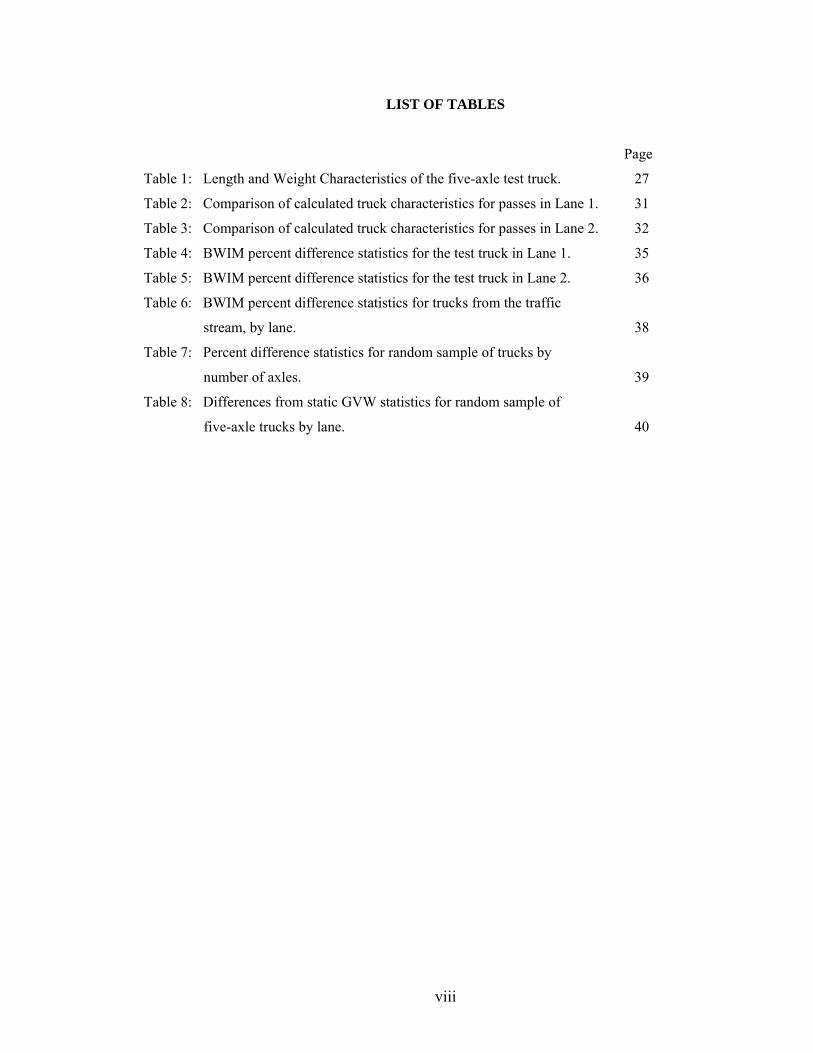
LIST OF TABLES

Page

Table 1: Length and Weight Characteristics of the five-axle test truck. 27

Table 2: Comparison of calculated truck characteristics for passes in Lane 1. 31

Table 3: Comparison of calculated truck characteristics for passes in Lane 2. 32

Table 4: BWIM percent difference statistics for the test truck in Lane 1. 35

Table 5: BWIM percent difference statistics for the test truck in Lane 2. 36

Table 6: BWIM percent difference statistics for trucks from the traffic

stream, by lane. 38

Table 7: Percent difference statistics for random sample of trucks by

number of axles. 39

Table 8: Differences from static GVW statistics for random sample of

five-axle trucks by lane. 40

1

INTRODUCTION Bridges are critical components to the transportation system. There are close to 600,000

highway bridges in the United States, with approximately 3,700 in Connecticut (ConnDOT,

2009). It is paramount that bridge structures are kept in functional condition. Failure of a

bridge can be a catastrophic event. The failure of a bridge can cause more than just structural

damage, including loss of life and public loss of confidence in the transportation

infrastructure. The Mianus River Bridge collapse in Greenwich, Connecticut in 1983 was

tragic. The Interstate-35W bridge failure in Minneapolis on August 1, 2007, is a recent

reminder of the importance of highway bridges in today’s society.

Understanding the dynamic loading on a bridge can help to correctly rate and maintain

bridges and the transportation infrastructure as a whole. Rating a bridge is the process of

calculating the maximum load a particular bridge can safely handle either on a daily basis or

for a one time loading. Live loads resulting from trucks have a more significant long-term

effect on the bridge safe life than a passenger car.

Information on truck weight data is important for many functions of maintaining the

infrastructure and transportation network. These functions include pavement design and

maintenance, enforcement, freight movement, traffic monitoring, air quality models,

determining remaining life of critical fatigue details, tracking weight limits on posted bridges,

and research.

Weigh-in-motion (WIM) is the process of estimating a moving vehicle's gross weight

and the portion of that weight that is carried by each wheel, axle or axle group or combination

thereof, by measurement and analysis of dynamic vehicle tire forces (ASTM International,

2

2009). WIM systems typically use sensors installed in the pavement to determine vehicle

characteristics, including gross weight, speed, axle weights, and axle spacing.

WIM systems utilize different sensor technologies, depending upon various factors

including application, environment, cost, and desired accuracy (Yannis and Antoniou, 2005).

The common WIM sensor technologies include piezoelectric systems, bending plates, and

load cells. Quartz-piezoelectric WIM systems are used for research and enforcement

applications in Connecticut (CASE, 2008). Polymeric piezoelectric sensor technologies are

used by ConnDOT for FHWA data collection and support of planning and engineering

applications (CASE, 2008).

There have been many initiatives that have contributed to the improvement of WIM

accuracy in recent years. In Europe, the Weigh-In-Motion of Axles and Vehicles for Europe

(WAVE) project was a significant advancement (WAVE, 2001). In addition, considerable

work conducted under the COST (European Cooperation in Science and Technology) project

323 resulted in numerous improvements, including guidelines for WIM referred to as COST

323 Specifications (COST 323, 2002). COST 323 includes a standardized method for

classifying the accuracy of a WIM system.

In the United States, there have been several initiatives that have resulted in the

improvement and focus on weigh-in-motion. ASTM standard specifications E-1318 (09)

“Standard Specification for Highway Weigh-In-Motion (WIM Systems with User

Requirements and Test Methods)” is the primary specification used for WIM systems in the

United States (ASTM International, 2009). AASHTO designated weigh-in-motion as a

concept of focus technology in 2004 (http://tig.transportation.org/?siteid=57&pageid=1003,

November 18, 2009). The work conducted under the FHWA-LTPP Long Term Pavement

3

Performance Program (LTPP) as lead to collection of research quality data through improved

practices including specific installation, calibration and data validation procedures.

The International Society for Weigh-In-Motion (ISWIM) is an international society

comprised of researchers, manufacturers and end users of WIM technology (ISWIM, 2007).

ISWIM was established to support multiple aspects of WIM, including advances in WIM

technologies, standardization of WIM technologies, a more widespread use of WIM, and the

applications of WIM data.

Despite these best efforts to improve the standard practices, there are challenges

associated with use of current WIM technologies. The common challenge for all of the types

of WIM sensors is their placement in the road surface. The majority of technologies require

sensors that are embedded in the pavement and require pavement cuts or some form of

excavation. Other systems that place or adhere sensors on the pavement present different

challenges. Both methods require working in the lanes of traffic. This makes the WIM

systems both dangerous and costly to install and maintain. Pavement smoothness is a critical

factor for in-pavement (and on-pavement) WIM systems to produce accurate results. This is

necessary to minimize the influence of vehicle dynamics. It is difficult to build and maintain

pavements that are sufficiently smooth throughout the WIM approach and installation.

Bridge weigh-in-motion (BWIM) is an alternative to traditional WIM. BWIM uses

the response of a bridge to determine WIM data. BWIM has potential to produce similar

results as traditional WIM, while overcoming the challenges associated with sensors in the

pavement. BWIM is potentially less sensitive to vehicle dynamics than traditional WIM.

BWIM was first proposed by Moses in the 1970’s (Goble, et al., 1976; and Moses, 1979).

4

Recent advances in sensor technology and data acquisition hardware and software capabilities

can allow for improvements in the accuracy and application of BWIM.

This study proposes an automated BWIM methodology made possible by use of state-

of-the-art bridge monitoring sensor and data acquisition technologies. A literature review of

existing BWIM technology was first conducted. The proposed methodology utilizes strain

sensors that are mounted underneath a single-span steel-girder bridge. A test vehicle was used

as the control for calibration. A field study was conducted to validate the BWIM methodology

recording bridge strain measurements of reference truck traffic traveling on an in-service

Connecticut Interstate. The trucks are then measured at a nearby weigh station. The strain data

is processed to determine the gross vehicle weight, axle spacing, axle weights, and speed of

individual trucks crossing the bridge. The accuracy of the proposed BWIM results is

evaluated.

LITERATURE REVIEW

The concept of bridge weigh-in-motion was proposed over 30 years ago (Goble, et al.,

1976; Moses, 1979). An initial BWIM system was developed in 1979 that required sensors

both on the pavement and beneath the bridge. The pavement sensors were used to determine

vehicle speed and axle spacing. Strain sensors located beneath the bridge were used to

compare strain time histories to calculated influence lines from a model of the bridge. A field

test of this system reported that the gross vehicle weight of the calibration truck from twelve

crossings generated an 11% error for a 95% confidence interval. It demonstrated that truck

weight predictions from strain measurements were feasible (Moses, 1979). Subsequent

BWIM methods continued to be based on influence lines. These methods require an inverse

matrix solution to produce individual axle weights (Snyder and Moses, 1985). This innovative

5

system was groundbreaking for bridge weigh-in-motion. The drawbacks included that

determining the influence lines for an in-service bridge can be challenging and requires an

accurate model of the bridge structure. Additionally, sensors located in the pavement can be a

safety issue for installation and maintenance. This system was not easily implemented.

In 1999, O’Brien (O’Brien, et al., 1999) made the transition from requiring an actual

influence line for each bridge to only needing a theoretical influence line for bridge WIM.

This simplified the testing process as the theoretical influence line is scaled up or down

depending upon the calibration truck results.

A more recent procedure to determine gross vehicle weight requires no estimation of

influence lines, but instead consists of integrating the strain response data, adjusting for speed,

and using a calibration factor identified from a test truck to determine gross vehicle weights

(Ojio and Yamada, 2002). In a 2006 field test, this method was employed to demonstrate

feasibility of BWIM on a multi-span steel girder bridge in Connecticut (Cardini and DeWolf,

2009). Cardini and DeWolf illustrated that BWIM can be achieved using an existing bridge

monitoring system.

BWIM methodologies have adopted a non-intrusive approach whereby no sensors are

placed in the pavement – Non-intrusive is also known as Nothing-On-the-Road (NOR) or

Free-of-Axle Detector (FAD). The non-intrusive method eliminates the use of pneumatic

tubes or tape switches in the travel lanes. Neural network-based methods are also employed to

remove the need for intrusive devices on the roadway. A comparison study between three

types of neural network systems used for classifying trucks passing over a bridge was

conducted by Flood (2000). The study demonstrated the viability of using neural networks

for truck classification using the Federal Highway Administration (FHWA) system. More

6

recent testing, conducted by Chatterjee, et al. (2006), uses a wavelet-based approach to

analyze the strain signals, which can also produce vehicle speed, axle spacing, axle weights,

and gross vehicle weights. Truck speeds for Cardini and DeWolf (2007) were manually

calculated in their non-intrusive application by examining the time delay between the peak

strain responses of multiple adjacent spans.

The SiWIM system is the result of research conducted in Slovenia on BWIM

(Žnidarič, et al., 2002). SiWIM is a commercially available BWIM system that has been

deployed extensively for short-term BWIM applications.

The most recent application of BWIM in the United States was in Alabama using a

commercially available SiWIM BWIM system. The application of the SiWIM system in

Alabama was the focus of a recent FHWA-funded research project between the Alabama

Department of Transportation and the University of Alabama – Birmingham (UTCA, 2007).

The results of this testing are not yet available in open literature.

The literature indicates many applications where the need to determine the weights of

moving vehicles from bridge weigh-in-motion is useful. Examples of these include

prescreening, bridge rating, and health monitoring. Notably, Nyman and Moses (1985)

applied BWIM data to structures to design a bridge prescreening tool. More recently, the

portable SiWIM system has been used in Slovenia and France as a prescreening tool for

temporary weight enforcement. Ghosn, et al. (1986) used BWIM to assist in bridge rating and

evaluation. Similarly, Swan and Fairfield (2008) implemented a BWIM system to monitor the

condition of the bridge involved in testing.

7

PROPOSED BWIM METHODOLOGY

The proposed methodology uses strain measurements on a slab-on-girder highway bridge to

determine gross vehicle weight, speed, axle spacing, and axle weights. This method does not

require development of a bridge model or influence line. The unique aspect of the proposed

BWIM method in this study is the non-intrusive calculation of truck characteristics for a

single span highway bridge using only strain measurements of the steel girders beneath the

bridge. The proposed method builds on the theory for determining gross-vehicle weight from

the work of Ojio and Yamada (2002) and the findings of Cardini and DeWolf (2002). The

strain sensors are located on the steel girders beneath the bridge and are non-intrusive (i.e. no

sensors in the pavement). The bridge used for testing has just one span and can be assumed to

behave as a simply supported beam. While this approach neglects the spatial behavior of the

multi-lane bridge, examining girders located directly under the lanes of travel allows for the

simply supported beam assumption. Vehicle loads are applied to the bridge by the truck axles

and can be modeled as a group of point loads moving across the simply supported beam at

fixed spacing and constant speed.

A schematic of the simply supported beam is shown in Figure (Fig.) 1.

Figure 1: Simply supported beam with point load representing a single span bridge with axle loading.

x P

L

A C

B · · ·

8

The largest internal moment for a point load moving over a simply supported beam

occurs at midspan, C. The influence line for the moment at the midspan shows the variation

of the moment due to the application of a unit load at various distances along the length of the

beam. The influence line for the moment at the middle of the span (mid-span) and the

corresponding equations are shown in Fig. 2 and Equation (Eq.) (1) (AISC, 2005).

Figure 2: Influence line for moment at the mid-span of a simple beam.

LxL

Lx

LxPL

Px

M c

<<

<<

⎪⎪⎩

⎪⎪⎨

⎧

⎟⎠⎞

⎜⎝⎛ −

=

2

20

12

2 (1)

where Mc is the internal moment at point C, P is the magnitude of the point load, x is the

distance from A to the location of the point load, and L is the total length of the beam.

The internal moment at a cross-section results in a stress distribution that can be

described by

IMc

=σ (2)

where σ is the stress, M is the internal moment, c is the distance from the sensor location to

the centroid of the cross-section, and I is the moment of inertia of the cross-section. While the

moment may not be available as a measurement, the strain at the midspan cross-section is an

x

Mc

9

available measurement in bridge monitoring. The strain in Eq. (2) can be written as a function

of the moment using Hooke’s Law ( εσ E= ) such that

EIMc

=ε (3)

where ε is the strain and E is the modulus of elasticity. Substituting Eq. (1) into Eq. (3) gives

LxL

Lx

Lx

EIPcL

EIPcx

xc

<<

<<

⎪⎪⎩

⎪⎪⎨

⎧

−=

2

20

)1(2

2)(ε (4)

Assuming the point load travels at a constant speed, v, over the bridge, distance can be

converted into time, t, as vtx = . The strain at midspan C from Eq. (4) can be rewritten as a

function of time as

vLt

vL

vLt

Lvt

EIPcL

EIPcvt

tc

<<

<<

⎪⎪⎩

⎪⎪⎨

⎧

−=

2

20

)1(2

2)(ε (5)

The first time derivative of the strain measurement is

vLt

vL

vLt

EIPcv

EIPcv

tdt

d c

<<

<<

⎪⎪⎩

⎪⎪⎨

⎧

−=

2

20

2

2)(ε

(6)

If discrete samples of the strain are measured, at time interval ∆t, the second time derivative

of the strain measurement can be written as

10

⎪⎪⎪

⎩

⎪⎪⎪

⎨

⎧

Δ−

Δ

=

0

2

)(2

2

tEIPcv

tEIPcv

tdt

d cε

elsewherev

Lt

vLandt

2

0

=

=

(7)

The strain and its associated time derivatives are illustrated in Fig. 3 as functions of time.

Figure 3: The strain and associated derivatives of a simply supported beam with a moving point load.

The strain at any location along the length of the beam will take the same form as in

Eq. (5), with reduced amplitude. As such, the subscript c denoting the strain at the mid-span

of the beam can be dropped. Furthermore, the strain due to any magnitude point load will take

the same form amplified by the relative magnitude of the point load. Superposition can be

used to account for more than one axle (point load) such that the strain and associated

derivatives can be written as:

t

ε

t

t d2ε dt2

dε dt

11

∑=

−=N

nnn tt

1)(εε (8)

∑=

−=N

nn

n ttdt

ddtd

1

)(εε (9)

∑=

−=N

nn

n ttdt

ddtd

12

2

2

2

)(εε (10)

where N is the number of axles (point loads), εn is the strain for an individual axle, and tn is

the time between when the first axle enters the bridge and the nth axle reaches the midspan of

the bridge. Fig. 4 depicts the effect of multiple point loads as it illustrates the theoretical

influence line and associated derivatives for a typical five-axle truck traveling over a 26.0 m

(85.3 ft) span at 25.0 m/s (55.9 mph). For the purpose of generating Fig. 4, the weights of

axles one through five are estimated for this example to 45.0 kN, 60.0 kN, 60.0 kN, 70.0 kN,

and 70.0 kN (10.12 kips, 13.49 kips, 13.49 kips, 15.74 kips, and 15.74 kips), respectively.

The corresponding distances between axles are 3.60 m, 1.35 m, 7.40 m, and 1.20 m. The

dashed peaks in the first plot represent the strain from each individual axle load. The varying

heights of these peaks are a result of the magnitude of the point loads. The summation of the

strain caused by all five axles produces the larger peak (solid line). The shape is unique to the

axle spacing and relative weights.

12

Figure 4: Theoretical response wave and associated derivatives as functions of time.

ε

t

dε dt t

d2ε dt2 t

t2

t3

t1

t4

t5

t0

total response

1st point load

5th point load 4th point load

3rd point load 2nd point load

13

The second (4B) and third (4C) plots in Fig. 4 represent the first and second

derivatives of the strain with respect to time. It should be noted that at other

measurement locations on the beam the general shape of the strain and derivatives of

strain only change in amplitude. The peak values in strain occur when the axle crosses the

midspan, regardless of the measurement location on the length of the beam.

Calculating the vehicle speed is the first and a vital step to calculating the gross

vehicle weight, axle spacing, and axle weights. This study uses only strain measurements

from sensors underneath the bridge to determine the vehicle speed. The second derivative

of the strain exhibits impulses when the axle loads enter the span, cross the middle of the

span, and exit the span. The first five positive peaks (Figure 4) correspond to the times

when the five axles enter the span. The five negative peaks correspond to the times t1

through t5 when each axle passes over the middle of the span. The final five positive

peaks and the final recorded time correspond to the times when each axle exits the span.

It should be noted that the negative peaks of the second derivative (Figure 4B)

correspond to the axles passing over the middle of the span are twice as large as the

positive peaks corresponding to the axles entering and leaving the bridge.

Truck speed is determined from the time it takes the first-axle to pass two fixed

points, specifically the initial point (start) on the bridge deck and mid-span of the bridge.

The strain gauge records the time the time it takes the first axle to reach the mid-span of

the bridge and the distance traveled in this time is known. As such, speed is determined

as half the span length, L/2, divided by time t1. The equation to calculate the truck’s

speed is

)(2 1tLv = (11)

14

where v is the speed of the truck (m/sec), L is the length (m) and t1 is the time it takes for

the first axle of the truck to travel from the start of the bridge to the mid-span.

The second derivative of the strain (Figure 4 B) provides the times when each of

the remaining axles pass over the mid-span of the bridge; t2, t3, t4 and t5. The product of

time difference between these times and the calculated speed provides the truck’s axle

spacing, dn. The equation for axle spacing is

)( 1 nnn ttvd −= + , n= 1,2,…,N-1 (12)

where dn is the distance between the n-1 and nth axles, and tn is the time it takes for the nth

axle to reach the mid-span of the bridge after the truck first enters the bridge, and N is the

total number of axles on the truck.

Gross vehicle weight is determined from the method of Ojio and Yamada (2002).

The response wave is the strain response of the bridge to a truck traveling over the

bridge. The response wave can be defined mathematically as the strain at a specific

location of the bridge due to multiple point loads traveling over the bridge. The response

wave is written as

( ) ∑=

−=N

nnn xxfPx

1)(ε (13)

where Pn is the weight, or magnitude, of the nth axle, assumed to be a point load P, xn is

the distance between axles, and )( nxxf − is the influence line of the simply supported

beam as defined as LxL

Lx

Lx

EIcLEIcx

xf<<

<<

⎪⎪⎩

⎪⎪⎨

⎧

⎟⎠⎞

⎜⎝⎛ −

=

2

20

12

2)( .

15

The influence area, A, of a single truck passing over the bridge is defined as

( ) ( )dxxxA ∫∞

∞−

= ε (14)

Substituting Eq. 13 into Eq. 14 and rearranging slightly gives

∑ ∫=

∞

∞−

−=N

nnn dxxxfPA

1

)( (15)

Recognizing that the Gross Vehicle Weight (GVW) can be written as

∑=

=N

nnPGVW

1 (16)

allows Eq. (15) to be simplified as

∑ ∫=

∞

∞−

−=N

nn dxxxfGVWA

1)( (17)

For trucks with the same axles configuration the term in the summation is a constant,

such that

∑ ∫=

∞

∞−

−=N

nn dxxxf

1)(α (18)

This constant α can be substituted into Eq. (17) and written as

α=GVW

A (19)

If the GVW of test truck is known, the GVW of any second truck can be determined

knowing that

u

u

k

k

GVWA

GVWA

= (20)

16

where Ak and GVWk are the calculated area and reference gross vehicle weight for a test

truck of known weight, and Au and GVWu are the calculated area and gross vehicle weight

for a truck with unknown weight.

Equation (20) can be arranged so that

kk

uu GVW

AA

GVW = (21)

The ratio of GVWk to Ak is defined as the calibration constant β where

k

k

AGVW

=β (22)

that the GVW of the unknown truck is then determined as

βuu AGVW = (23)

where A can be written in terms of ε(t), again where vtx = , and written in discrete form

such that

( ) ( )∑∫=

∞

∞−

ΔΔ

==N

i

tiN

tvdttvtA1

)( εε (24)

where Δt is the discrete sample time of the strain measurement, and N is the total number

of measurements needed for the truck to cross the bridge. It should be noted that the

method of Ojio and Yamada (2002) does not incorporate the dynamic effects of the

bridge response in the calculation of GVW.

As part of this study, the axle weights are then determined from the GVW and

strain measurements. For this methodology the point loads, Pn, are assumed to be

equivalent to the axle weights. Distributing the GVW into axle weights is done by

recognizing that the amplitude of 2

2

dtd ε is directly proportional to the axle load, Pn, where:

17

tEIcvP

tdtd n

n Δ−=)(2

2ε (25)

If the constant tEI

cvΔ

−=Γ is defined, then

Γ= nn Ptdtd )(2

2ε (26)

The sum of this quantity over all axles results in

∑∑==

Γ×=Γ=N

nn

N

nn GVWPt

dtd

112

2

)(ε (27)

Dividing Eq. (26) by Eq. (27) gives

GVWP

GVWP

tdtd

tdtd

nnN

nn

n

=Γ×

Γ=

∑=1

2

2

2

2

)(

)(

ε

ε

(28)

As such the nth axle weight, Pn, can be calculated as

GVWt

dtd

tdtd

PN

nn

n

n ×

⎥⎥⎥⎥

⎦

⎤

⎢⎢⎢⎢

⎣

⎡

=

∑=1

2

2

2

2

)(

)(

ε

ε

(29)

As such, the gross vehicle weight, speed, axle spacing, and axle weights are

determined in this section from the time history measurement of the strain using Eqs.

(21), (11), (12), and (29), respectively. In particular, the unique aspects of the

methodology proposed in this study are the calculation of speed and axle weight from the

second time derivative of the strain measurement.

18

The BWIM methodology produces calculated speed, GVW, axle spacing and axle

weight data. These BWIM results will be referred to as BWIM-speed, BWIM-GVW,

BWIM-axle spacing and BWIM-axle weight.

FIELD STUDY VALIDATION OF BWIM METHODOLOGY

Field testing to validate the proposed BWIM methodology took place on November 20,

2008. The field study was set up to collect bridge response data both for multiple passes

of a test truck of known-weight, speed and configuration, and bridge response data and

static weights and measurements for trucks from the traffic stream. The test truck results

were used to both calibrate and validate the BWIM system. The BWIM results for the

trucks from the traffic stream were then correlated to measured weights from the static

scale and axle spacing measured from still digital photos at a static weigh station. The

static weigh station is located a half mile north of the bridge and is operated by the

Connecticut State Police. Data sets of traffic stream data were collected according to a

coordinated effort with the State Police for intervals of when the weigh station was open.

In all, eight sets of truck data were collected for a total of 163 passes from the traffic

stream. A statistical analysis was conducted to quantify the performance of the BWIM

system and identify the 95% confidence intervals of the various measurements. The

change in temperature, as measured on the surface of the steel bridge girders, was less

than 8o F over the course of the testing. As such, the effect of temperature on the strain

measurements is neglected. This chapter describes the main components of the field

study, namely the highway bridge, static scale, bridge monitoring system, and the

characteristics of the truck traffic used for the field study.

19

Highway Bridge

The bridge used in this research is located on Interstate 91 (I-91) Northbound over

Baldwin Avenue in Meriden, Connecticut. The bridge, denoted Bridge Number 03051,

was built in 1964. The bridge was inspected on August 12, 2008, three months prior to

the field data and received a sufficiency rating of 96 out of 100. The sufficiency rating

indicates a bridge’s sufficiency to remain in service, where 100 is entirely sufficient. The

formula for the sufficiency rating (FHWA, 1995) is used to determine if a bridge is

eligible for Federal funding eligibility for maintenance, rehabilitation, or replacement

(e.g. a bridge with a sufficiency rating of 80 or less is eligible for Federal bridge

rehabilitation funding; and a sufficiency rating of 50 or less is eligible for Federal bridge

replacement funding). The Meriden Bridge is sufficient to remain in service and

furthermore meets desired conditions for the BWIM field study, including proximity to a

permanent weigh station, a smooth approach, access to install sensors, and little skew.

Truck flow during testing remained steady and averaged over 200 trucks each hour.

Figure 5 displays the location of the highway bridge relative to the weigh station, and

Fig. 6 shows the road surface of the bridge.

The bridge’s layout and geometry are of importance. Since it is the feasibility of

BWIM being assessed, it is important to select a structure with a simple layout and a

noncomplex geometry for initial testing. A flat, short, straight, and single span steel

girder bridge is ideal for BWIM testing. The selected highway bridge, illustrated in Fig.

7, closely matches these ideal characteristics while also being in close proximity to a

truck weight station.

20

Weigh Station

Bridge

Figure 5: Aerial view of bridge in relation to weigh station on I-91N.

Figure 6: View of the bridge’s road surface.

Figure 7: East elevation view of bridge over Baldwin Avenue.

21

The bridge is a 25.91 m (85 foot) single-span with multiple plates stringers

supported by bearings. The out-to-out width is 16.76 m (55 feet), which is designed for

three lanes of traffic 3.66 m (12 feet) each. In Connecticut trucks drive legally in two

right lanes of the three-lane roadway. When two trucks travel closely, either bumper-to-

bumper following in the same lane, or parallel in adjacent lanes post-processing

difficulties are encountered. During this test, two closely traveling trucks were found to

be uncommon, occurring less than 5% of the total passes.

Three important geometric aspects for BWIM are the slope of the roadway, the

curve of the roadway, and the skew of the bridge itself. There is a +2.56% longitudinal

slope on the bridge. The bridge is located on a straight portion of the highway, but the

roadway below forced the bridge to have an 11.5° skew. Previous research has shown

that a skew up to 26º has a minor impact on accuracy of BWIM (WAVE, 2001).

The bridge has appropriate access to the desired sensor locations on the steel

girders beneath the bridge shown in Fig. 8.

Figure 8: View of the steel girders and underside of the bridge.

22

Weigh Station

The State of Connecticut, Department of Public Safety operates a weigh station

located on Interstate-91 (I-91) Northbound in the town of Middletown, Connecticut. The

weigh station is located 0.8 km (0.5 miles) north of the bridge instrumented for the test,

as shown in Fig. 5. The trucks are required to report for static weight measurements when

the station "OPEN" sign is lighted. Data collection was coordinated between the bridge

and weigh station using synchronized video recordings that were manually reviewed to

match vehicle to vehicle results. Still photos of each truck at the weigh station were used

to measure the axle spacing. Calculated GVW from the BWIM system were compared

with static weights and axle spacing of the trucks recorded at the weigh station in

order to determine the level of accuracy of the system. The static scales at the weigh

station were calibrated by the manufacturer one week prior to testing, shown in Fig 12.

The static scale consists of three platforms, shown in Fig. 13. The first platform weighs

the first axle, the second platform the second axle and the third platform weighs the

remaining axles. With only three platforms, all trucks, no matter how many axles,

generate three load values. The axle weights are summed together to get the gross

vehicle weight.

23

23

Figure 9: Cross-section view of the bridge and sensor layout (red dots).

Figure 10: Plan view of the highway bridge.

Figure 11: Elevation view of a typical steel girder.

24

Figure 12: Calibrating the scales at the static weight station.

Figure 13: View of the three platforms at the static weigh station.

12

3

25

Bridge Monitoring System

The monitoring system used for this testing is the Bridge Diagnostics

Incorporated STS–WiFi System. The system shown in Fig. 14 consists of eight strain

sensors which can be temporarily installed onto the bridge.

Figure 14: Bridge monitoring system used during testing. The sensor and data acquisition system consists of eight strain sensors, two nodes,

and one base station. Strain transducers are permanently attached to wires ranging from

4.57 to 7.62 m (15 to 25 feet) in length. These wires plug into one of two nodes holding

up to four sensors. The two nodes then wirelessly transmit strain measurements to a

small base station nearby. The base station collects data from both nodes and broadcasts

all the data wirelessly to a laptop with the appropriate software.

Fig. 15 presents the eight strain sensor locations, as well as the locations of the

two nodes on the steel girders. The base station was located at ground level below the

bridge. There was also a data collecting station as part of the bridge monitoring system

on the side of the highway just north of the bridge which is where the laptop was located.

This configuration was devised as a result of trial and error to determine the optimum

26

range of the broadcast, as well as the ability to view traffic. The data acquisition system

was manually triggered at the data collecting station located by the bridge. Typical

testing intervals lasted five minutes with a frequency of 100 Hertz.

Base Station Laptop Figure 15: Plan view of the girder and sensor layout.

Truck Traffic

The truck traffic for this field study included a five-axle test truck in addition to

trucks from the traffic stream. Details of these trucks are presented in this section.

The fully loaded five-axle truck was used during testing as a test truck to calibrate

the BWIM system. The truck was loaded with a stable load. The test truck was statically

measured, as shown in Fig. 16, at the weigh station both before and after passes at the test

site. The test truck’s corresponding lengths and weights are presented in Table 1. The

27

test truck made a total of 10 passes over the bridge, five passes each in lane 1 and lane 2,

at various speeds ranging from 23.7 m/sec to 28.2 m/sec (55 to 65 mph). The test truck

passes are used for calibration.

Figure 16: Five-Axle Test Truck

Table 1: Length and Weight Characteristics of the five-axle test truck.

Gross Vehicle Weight 300.00 kN 67,420 lbs Wheelbase length

(first (1) to last (5) axle 13.58 m 44.57 feet

Length (bumper to bumper) 16.46 m 54 feet Number of Axles 5 5

Axle Spacing (1-2) 3.59 m 11.77 feet Axle Spacing (2-3) 1.34 m 4.40 feet Axle Spacing (3-4) 7.42 m 24.35 feet Axle Spacing (4-5) 1.23 m 4.05 feet

Axle Weight (1) 44.59 kN 10,020 lbs Axle Group Weight (2 & 3) 120.32 kN 27,040 lbs Axle Group Weight (4 & 5) 135.09 kN 30,360 lbs

The sample of 117 trucks from the traffic stream analyzed in this study consisted

of a variety of vehicles. Details on each vehicle are provided in the Appendix. Trucks

ranged from a two-axle 51.6 kN (11.6 kips) flatbed to a six-axle 445 kN (100 kips) truck

28

0

5

10

15

20

25

30

< 50 50-100 100-150 150-200 200-250 250-300 300-350 > 350

Weight Ranges (kN)

Num

ber o

f Tru

cks

transporting an excavator. Figure 17 shows the gross vehicle weight distribution of the

trucks from the traffic stream as determined from the weigh station static measurements.

Figure 17: Histogram of truck weights from the traffic stream.

PROCESSING AND CALIBRATION

A program was developed in MATLAB (ref) for the post-processing and calibration of

the field test data. In the MATLAB program the strain time histories are loaded, data

filtered, and truck crossing events identified automatically. Each truck event is processed

using the proposed BWIM methodology, as identified in the Proposed BWIM

Methodology section. The level of accuracy for the BWIM is quantified by comparing

the difference between the BWIM calculated and weigh station measured GVW, axle

spacing, and axle weights.

The fully automated program developed in MATLAB is used to determine the

speed, gross vehicle weight, axle spacing, and axle weight for trucks from the traffic

stream. The program obtains the raw strain data from each sensor. A typical five-

29

minute time history plot of strain at sensor 7 is shown in Fig. 18. An eight-pole low-pass

filter with a 15 Hertz cutoff frequency is used to reduce the effect of noise on the

derivatives of strain. Minimizing noise is especially important for calculating vehicle

speed. Speed is determined from the second derivative of strain versus time and results

are sensitive to high frequency components of the signal present from the measurement

noise.

Figure 18: Typical time history plot of strain with truck GVW indicated.

Time history plots of the strain and second time derivative of the strain are shown

in Figs. 19 and 20 for the three passes of the test truck traveling in Lane 1 at the same

speed.

30

Figure 19: Time history plot of the strain for three passes in Lane 1.

Figure 20: Time history plot for the second derivative of strain for the three passes.

The calibration constant, β, from Eqs. 22 and 23 is determined by trial and error

from the experimental results for the test truck to minimize mean difference between the

BWIM calculated GVW and the static scale measured GVW. Five passes of the test

31

truck, at various speeds, for each of the two lanes were used to establish the calibration

factor for each lane for trial and error. The calibration constants for this bridge using

strain sensor 7 for Lane 1 and strain sensor 2 for Lane 2 are: β1=0.6291m

kN⋅με

and

β2=0.6906m

kN⋅με

. Table 2 reports the measured values for all of the examined

characteristics of the test truck and compares them to the BWIM results for the five

passes in Lane 1. Table 3 provides the same comparison for the five passes in Lane 2.

The values of β calculated for the test truck are applied for BWIM for the trucks from the

traffic stream as reported in the following section of this report.

Table 2: Comparison of calculated truck characteristics for passes in Lane 1.

Pass Number Measured 1 2 3 4 5 GVW (kN) 300.00 300.64 293.10 305.25 292.13 308.91

Reported Speed (m/s) - 24.59 24.59 26.82 24.59 23.69

BWIM Speed (m/s) - 25.10 26.12 28.45 23.27 23.70

Wheelbase – sum of di (m) 13.58 14.81 15.15 13.09 13.97 14.70

Number of Axles 5 5 5 4 5 5 Axle Spacing –

d1 (m) 3.59 3.77 3.92 3.70 3.03 3.79

Axle Spacing – d2 (m) 1.34 1.76 1.83 1.42 2.09 1.66

Axle Spacing – d3 (m) 7.42 7.53 7.84 7.97 6.98 7.59

Axle Spacing – d4 (m) 1.23 1.76 1.57 - 1.86 1.66

Axle Weight – P1 (kN) 44.59 43.19 47.84 93.50 56.11 53.39

Axle Group Weight –

P2+P3 (kN) 120.32 140.56 149.38 138.67 103.18 149.41

Axle Group Weight –

P4+P5 (kN) 135.09 123.01 101.84 79.29 138.79 112.39

32

Table 3: Comparison of calculated truck characteristics for passes in Lane 2.

Pass Number Measured 1 2 3 4 5 GVW (kN) 300.00 299.21 316.14 273.09 315.94 295.71

Reported Speed (m/s) - 27.71 25.93 26.82 26.37 28.16

BWIM Speed (m/s) - 27.83 28.45 26.12 30.48 26.12

Wheelbase – sum of di (m) 13.58 16.42 15.08 15.68 14.02 15.68

Number of Axles 5 6 5 6 6 6 Axle Spacing –

d1 (m) 3.59 3.90 3.98 3.40 3.35 3.66

Axle Spacing – d2 (m) 1.34 1.67 1.71 1.83 2.44 1.83

Axle Spacing – d3 (m) 7.42 7.79 7.97 7.32 1.83 6.53

Axle Spacing – d4 (m) 1.23 1.11 1.42 1.05 2.44 1.57

Axle Weight – P1 (kN) 44.59 38.01 50.78 52.10 95.11 8.77

Axle Group Weight –

P2+P3 (kN) 120.32 27.69 189.47 31.32 150.96 138.26

Axle Group Weight –

P4+P5 (kN) 135.09 237.57 80.20 193.39 74.18 152.71

The test truck passes provided an opportunity to examine the accuracy of the

speed calculation. The BWIM calculated speed is compared to the speed identified by the

operator of the test truck reading of the speedometer when crossing the test site. For Lane

1, the speed calculation is between 0.01 m/sec and 1.63 m/sec magnitude difference from

the reported speed. For Lane 2, the speed calculation is between 0.12 m/sec and 4.11

m/sec magnitude difference from the reported speed. The calculated speeds are plotted in

Fig. 22 against the reported truck speeds identified by the operator of the test truck

reading of the speedometer when crossing the test site. The pass numbers are numbered

sequentially, so the first five passes are for Lane 1 and next five passes, reported 6-10, are

for Lane 2.

33

0

5

10

15

20

25

30

35

0 1 2 3 4 5 6 7 8 9 10

Pass Number

Velo

city

(m/s

)

Actual Velocity

BWIM Velocity

Figure 22: Plot of calculated speeds for the test truck (1-5 lane 1; 6-10 lane 2).

Noting that the influence area, Au, is directly proportional to the speed, and thus

the gross vehicle weight is directly proportional to the predicted speed, reveals the

importance of accurately predicting speed. Adjacent or leading/following vehicles,

including non-truck traffic, are observed to add error to the identification of the time

when the vehicle enters the bridge and/or the first axle crosses the mid-span of the bridge

span.

ACCURACY OF BWIM FIELD STUDY

The accuracy of the BWIM methodology proposed here is evaluated for the trucks from

the traffic stream. Accuracy for WIM systems is defined by the closeness or degree of

agreement of an estimated value to an accepted reference value, measured as the 95%

confidence intervals (95% compliance) of the difference in the estimated and reference

34

values as a percent of the reference value (ASTM, 2009). The BWIM accuracy is defined

as the difference in the BWIM measurement compared to the measurement taken at the

static scale as a percent of the static scale measurement and is calculated as

( )100×

−=

static

staticBWIMGVW

GVWGVWGVW

E (30)

where GVWBWIM is the gross vehicle weight as determined by the BWIM, GVWstatic is the

gross vehicle weight as determined by the static scale. Note that while EGVW is defined in

Eq. (30) for the GVW, it is similarly defined for the wheelbase, axle spacing, and axle

weights.

The sample mean, μ, of the value of interest is calculated as

∑=

=n

iiE

n 1

1μ (30)

where Ei is the ith vehicle characteristic difference as defined in Eq. (30), and n is the

number of samples. The sample variance, s2, is then calculated as

2

1

2 )()1(

1 ∑=

−−

=n

iiE

ns μ (31)

When n ≥ 20 the sample variance is a good estimator of the population variance.

The BWIM measurement should contain no bias and, therefore, a mean of the

difference that is close to zero. To ensure that the mean value of the difference is

sufficiently close to zero, the 95% confidence interval of the mean, with unknown

variance, is determined assuming the underlying population is Gaussian using the t-

distribution as

⎥⎦

⎤⎢⎣

⎡+−=⟩⟨ −−− n

stnst nn 1,2/1,2/1 ; ααα μμμ (32)

35

where tα/2,n-1 are p-percentile values of the t-distribution. For 95% confidence intervals,

α = 0.05, n = 117, and t0.025,117 = 1.98. The interval around the mean indicates an accurate

scale if the interval includes the value zero (Strathman, 1998).

The accuracy of the BWIM measurements can be defined by the 95% confidence

interval of the difference. The confidence interval indicates that 95 out of 100 of the

BWIM calculated truck characteristics will have a measurement difference within this

range (Ang and Tang, 1975). The 95% confidence interval of the BWIM characteristic is

⎥⎦

⎤⎢⎣

⎡+−=⟩⟨ −−− ststE nn 1,2/1,2/1 ; ααα μμ (33)

Applying this probabilistic analysis of the BWIM data, the data from the test truck

is first evaluated. The results from the 10 test truck runs, five passes in Lane 1 and five

passes in Lane 2, are presented in Tables 4 and 5, respectively. It should be noted that

when the number of samples is less than 10, as is the case here, the confidence intervals

obtained will be very approximate. However, the analysis for the test truck runs do

provide a basis for comparison of both lane accuracy and ultimately accuracy of the

method when applied to similar and varying truck configurations.

Table 4: BWIM percent difference statistics for the test truck in Lane 1.

Difference μ s <µ>0.95 <E>0.95 GVW [%] 0.00 2.45 [-3.05 3.05] [-6.31; 6.31]

Axle Weight (P1) [%] 31.88 44.91 [-23.89; 87.65] [-83.59; 147.36]Axle Group Weight (P2+ P3) [%] 13.23 15.90 [-6.51; 32.97] [-27.64; 54.11] Axle Group Weight (P4+ P5) [%] -17.79 16.58 [-38.38; 2.81] [-60.43; 24.85]

Wheelbase (sum of di) [m] 0.76 0.82 [-0.26; 1.79] [-1.35; 2.88] Axle Spacing (d1) [m] 0.05 0.35 [-0.38; 0.49] [-0.85; 0.95] Axle Spacing (d2) [m] 0.41 0.24 [0.11; 0.72] [-0.22; 1.04] Axle Spacing (d3) [m] 0.16 0.38 [-0.31; 0.64] [-0.82; 1.14] Axle Spacing (d4) [m] 0.14 0.77 [-0.82;1.10] [-1.85; 2.13]

36

Table 5: BWIM percent difference statistics for the test truck in Lane 2.

Percent Difference μ s <µ>0.95 <E>0.95 GVW [%] 0.01 5.91 [-7.33; 7.34] [-15.19; 15.20]

Axle Weight (P1) [%] 9.79 69.83 [-76.92; 96.49] [–169.75; 189.32] Axle Group Weight (P2+ P3) [%] -10.62 61.25 [-86.68; 65.43] [–168.11; 146.86] Axle Group Weight (P4+ P5) [%] 9.27 52.54 [-55.97; 74.51] [-125.81; 144.35]

Wheelbase (sum of di) [m] 1.80 0.89 [0.68; 2.91] [-0.50; 4.10] Axle Spacing (d1) [m] 0.07 0.28 [-0.29; 0.42] [-0.66; 0.80] Axle Spacing (d2) [m] 0.56 0.31 [0.17; 0.94] [-0.25; 1.36] Axle Spacing (d3) [m] -1.13 2.55 [-4.30; 2.04] [-7.70; 5.43] Axle Spacing (d4) [m] 0.29 0.56 [-0.41; 0.98] [-1.15; 1.72]

For Lane 1, the mean of the GVW difference is 0 (as calibrated) and the 95%

confidence interval of the mean includes the value zero. In fact, the 95% confidence

interval of the means for all of the truck characteristics calculated include the value zero,

except for the percent difference of the axle spacing between the second and third axle,

which is a relatively short distance of 1.34 m. The 95% confidence interval for the

percent difference of BWIM GVW is +-6.31%. This is to say that 95 times out of 100 the

reference (static measured) GVW will be within 6.31% of the GVW calculated from the

bridge. The wheelbase estimate for Lane 1 has a 95% confidence interval of [-1.35 m;

2.88 m], which is to say that 95 out of 100 times the reference wheelbase will not be less

than 1.35 m (4.43 ft) of the calculated value nor more than 2.88m (9.45 ft) larger than the

calculated value. The axle weight estimates for Lane 1 have much less accuracy, with

95% confidence intervals of the difference on the order of 25%-150%.

For Lane 2, the mean of the GVW difference is 0.01% and the 95% confidence

interval of the mean includes the value zero. For Lane 2 the 95% confidence interval of

the means for all of the truck characteristics calculated include the value zero, except for

the percent difference of the axle spacing between the second and third axle, as for Lane

37

1, and for the Wheelbase. The 95% confidence interval for the percent difference of the

BWIM GVW for Lane 2 is +-15.2%. This is to say that 95 times out of 100 the reference

(static measured) GVW will be within 15.2% of the GVW calculated from this truck

traveling over Lane 2 of the bridge. The 95% confidence interval for GVW in Lane 2 is

over two times larger than the GVW calculated for the test truck traveling over Lane 1.

The other confidence intervals for Lane 2 are similarly larger than for Lane 1. This

increase in the 95% confidence interval for the test truck passes is an indication that the

measurements obtained for trucks traveling over the bridge in Lane 2 may not be as

accurate as for the trucks traveling in Lane 1. Additionally, further analysis in this report

will focus on the accuracy of the GVW estimates of the proposed BWIM method.

For the trucks from the traffic stream, 137 random trucks were measured crossing

over the bridge and successfully matched with static measurements at the weigh station.

All of these vehicles were traveling in Lanes 1 and 2. Of the 137 trucks, 6 trucks (4.4%

of 137) were identified as changing lanes while crossing over the bridge. Additionally,

there were six occurrences where multiple trucks were on the bridge at the same time.

This resulted in 12 occurrences (8.8% of 137) where two trucks in adjacent lanes were on

the bridge at the same time. Multiple presences of automobiles with trucks are not

separated out, as this is a regular occurrence. Vehicles switching lanes on the bridge and

cases of multiple trucks on the bridge at the same time were not considered in

determining accuracy. Since the proposed BWIM method is not able to accommodate

lane changes and multiple vehicles without further modifications, these 18 identified

trucks are not considered. Two of the remaining trucks (1.7% of 119) were found to have

erroneous calculated speeds; that are speeds greater than 40.23 m/sec (90 mph). These

38

0

50

100

150

200

250

300

350

400

450

0 50 100 150 200 250 300 350 400 450

BWIM GVW (kN)

Stat

ic G

VW (k

N)

two trucks are also not considered in determining accuracy of the BWIM method. The

remaining 117 trucks are evaluated for accuracy.

A table of the BWIM calculated and static scale measured results for the 117

trucks from the traffic stream is located in the Appendix of this report. The truck speeds

are calculated to be traveling an average speed of 26.36 m/sec (59 mph). The accuracy

for trucks traveling over the bridge are summarized in Table 5 and shown in Figure 23.

Table 6: BWIM percent difference statistics for trucks from the traffic stream, by lane.

Lane # Trucks μ s <μ>0.95 <E>0.95 1 109 -1.94 12.78 [-4.37; 0.48] [-27.28; 23.39] 2 8 6.23 19.72 [-10.25; 22.72] [-39.23; 51.70]

Figure 23: Plot of static measured GVW versus BWIM calculated GVW for the 117 trucks from both lanes of the traffic stream.

The mean of the GVW difference is -1.09% and 6.23% for Lanes 1 and 2,

respectively. The 95% confidence interval of the two mean estimates both includes the

value zero. The 95% confidence interval for the BWIM difference of the GVW of the 109

trucks traveling over Lane 1 is [-27.28%; 23.39%]. The 95% confidence interval for the

39

BWIM difference of the GVW of the eight trucks traveling over Lane 2 is [-39.23%;

51.7%]. As observed previously the confidence interval for Lane 2 GVW measurement

difference is larger than for Lane 1. This is likely due to the location of the steel girders

instrumented below Lanes 1 and 2. This increased interval range may also be attributed to

the low number of trucks traveling (i.e. small sample size) over Lane 2.

The BWIM GVW estimate is based on the assumption that the vehicles traveling

over the bridge are five-axle trucks with similar axle spacing and weights as the test

truck. Table 7 examines the accuracy of the BWIM method as a function of the number

of truck axles (considering both Lane 1 and Lane 2 together). The six-axle and seven-axle

trucks, one of each, are not considered in this analysis. It is observed, as expected, that

the 69 five-axle trucks have the smallest 95% confidence interval of [-20.24%; 20.20%].

The five-axle truck sample was not further delineated by subsets of the 5-axle vehicle

type. In contrast, the 18 two-axle trucks have a confidence interval over twice as large, [-

48.52%; 43.81%]. To compensate for this increase in difference multiple test trucks can

be employed in future work to calibrate the GVW estimate based on vehicle type.

Table 7: Percent difference statistics for random sample of trucks by number of axles (does not include one six-axle and one seven-axle truck).

Axles # Trucks μ s <μ>0.95 <E>0.95 5 69 -0.02 10.14 [-2.46; 2.41] [-20.24; 20.20] 4 16 -5.84 14.99 [2.15 -37.63] [-37.63; 25.95] 3 12 -2.97 12.39 [-10.84; 4.91] [-29.97; 24.04] 2 18 -2.35 21.97 [-13.28; 8.58] [-48.52; 43.81]

The BWIM GVW estimate is now examined for only five-axle trucks considering

the lane traveled. Table 8 examines the accuracy of the BWIM method for five-axle

trucks as a function of the lane. It is observed that the 64 five-axle trucks in Lane 1 have

40

the smallest 95% confidence interval of [-17.52%; 15.26%]. The five five-axle trucks in

Lane 2 have a 95% confidence interval calculated to be [-38.03%; 66.39%]. The ASTM

Standard Specifications for Highway Weigh-In-Motion Systems (2009) requires the

tolerance for 95% conformance for the percent difference of gross vehicle weight to be

±15% for a Type II system. For Lane 1 limited to five-axle trucks, the proposed BWIM

system nearly meets this requirement with a 95% confidence interval of [-17.52%;

15.26%].

Table 8: Differences from static GVW statistics for random sample of five-axle trucks by lane.

Lane # Trucks μ s <μ>0.95 <E>0.95 1 64 -1.13 8.22 [-3.18; 0.92] [-17.52; 15.26] 2 5 14.18 20.31 [-11.04; 39.39] [-38.03; 66.39]

CONCLUSION

This study demonstrates that a non-intrusive bridge weigh-in-motion system using only

strain measurements applied to a single span steel girder bridge can be used to produce

WIM data including gross vehicle weights, axle spacing, axle weights, and speed. This

was achieved by development of a new bridge WIM methodology that applied existing

approaches together with a novel approach to calculate vehicle speed and axle

displacements and weights. The bridge WIM methodology was automated to identify

truck events and calculate estimates from the strain response.

A field test was conducted on an in-service highway bridge. The field test

included calibration of the system using a five-axle test truck and application of these

BWIM methodology and calibration results on a random sample of 117 trucks from the

41

traffic stream to calculate BWIM estimates and to verify the methodology in comparison

to static measurements obtained for the same vehicles.

For the test truck, the 95% confidence interval for GVW is +-6.31% for Lane 1

and +-15.20% for Lane 2. It is observed that the BWIM estimates are more precise for

Lane 1 than Lane 2. This is likely due to the configuration of the instrumented girders

beneath the lanes of travel, as well as the location of Lane 2 on the cross section of the

bridge, with adjacent lanes on both sides.

The accuracy of the BWIM system is also evaluated for 117 trucks from the

traffic stream. From the random truck traffic set, it was observed that for five-axle trucks

travelling in Lane 1, which compose 55% of the 117 trucks, the 95% confidence interval

for the GVW difference is [-17.52%; 15.26%]. The accuracy of the system may be

dependent on the vehicle type used to calibrate the system. Employing a calibration

methodology that accounts for the various vehicle types (multiple trucks with varying

number of axles and spacing, suspensions, etc.) for calibration might reduce this

difference. Collecting more data for both the test truck(s) and for trucks in Lane 2 may

help to provide more confidence in the parameter estimates and ultimately the resulting

confidence intervals. Furthermore, as the BWIM GVW estimate is directly dependent on

speed, there is a need in future studies to more closely examine and consider the accuracy

of the speed estimate.

The initial field results reported in this study indicate that a non-intrusive BWIM

methodology shows great promise to achieve the tolerance of 95% probability of

conformity for Type II ASTM Standard Specifications for Highway Weigh-In-Motion

Systems.

42

REFERENCES

American Institute of Steel Construction (AISC). “Manual of Steel Construction – Load

and Resistance Factor Design.” Third Edition, (2005).

American Society for Testing and Materials (ASTM). “Standard Specification for

Highway Weigh-in-Motion (WIM) Systems with User Requirements and Test

Method.” ASTM E 1318-94, (1994).

Ang, A. and W. Tang. “Probability Concepts in Engineering Planning and Design.”

Volume 1 – Basic Principles, Wiley, (1975).

ASTM International. “Standard Specification for Highway Weigh-In-Motion (WIM)

Systems with User Requirements and Test Methods.” Designation: E 1318-09,

West Conshohocken, PA, (2009): 1-16.

Connecticut Academy of Science and Engineering (CASE). “A Study of Weigh Station

Technologies and Practices.” Authors D. Pines and C. Fang, CT-2257-F-08-7,

(2008).

Cardini, A. J. and J. T. DeWolf. “Development of a Long-Term Bridge Weigh-In-Motion

System for a Steel Girder Bridge in the Interstate Highway System.” University

of Connecticut, (2007).

Chatterjee, P., E. O’Brien, Y. Li, and A. Gonzalez. “Wavelet Domain Analysis for

Identification of Vehicle Axles from Bridge Measurements.” Computers and

Structures, 84, (2006): 1792-1801.

ConnDOT. “The Connecticut Department of Transportation.” Website (2009):

<http://www.ct.gov/dot /site/default.asp>

43

COST 323. “Weigh-in-Motion of Road Vehicles.” European WIM Specification – Final

Report, Paris, (2002).

Federal Highway Administration (FHWA). “Recording and Coding Guide for the

Structure Inventory and Appraisal of the Nation’s Bridges.” Report No. FHWA-

PD-96-001 (1995): 98 pages.

Flood, I. “Developments in Weigh-in-Motion Using Neural Nets.” Computing in Civil

and Building Engineering, Vol. 2, (2000): 1133-1140.

Ghosn, M., F. Moses, and J. Gobieski. “Evaluation of Steel Bridges Using In-Service

Testing.” Transportation Research Record, 1072, (1986): 71-78.

Goble, G.C., Moses, F., Pavia, A. “Applications of a Bridge Measurement System.”

Transportation Research Record, n 579, (1976): p 36-47.

Hwang, E. and D. Bae. “Calculation of Truck Weights by Bridge Diagnostic System.”

Key Engineering Materials, Vol. 270, (2004): 1478-1483.

ISWIM. “International Society for Weigh-In-Motion.” LCPC, Website (2007):

<http://iswim.free.fr/>.

Moses, F. “Weigh-in-Motion System Using Instrumented Bridges.” Transportation

Engineering Journal of ASCE, 105 (TE3), (1979): 233-249.

Nyman, W. and F. Moses. “Calibration of Bridge Fatigue Design Model.” Journal of

Structural Engineering, Vol. 111, (1985): 1251-1266.

O’Brien, E., A. Znidaric, and A. Dempsey. “Comparison of Two Independently

Developed Bridge Weigh-in-Motion Systems.” International Journal of Vehicle

Design. Heavy Vehicle Systems, Vol. 6, (1999): 147-161.

44

Ojio, T. and K. Yamada. “Bridge Weigh-In-Motion Systems Using Stringers of Plate

Girder Bridges,” Pre-Proceedings of the Third International Conference on

Weigh-In-Motion, (2002): 209-218.

Snyder, R. and F. Moses. “Application of In-Motion Weighing Using Instrumented

Bridges.” Transportation Research Record, 1048, (1985): 83-88.

Strathman, J.G. “The Oregon DOT Slow-Speed Weigh-in-Motion (SWIM) Project” Final

Report for the Oregon Department of Transportation Research Unit, State

Research #512, (1998), 64 pages.

Swan, I. and C. Fairfield. “The Dynamic Response of the Berwick-Upon-Tweed Bypass

Bridge.” Insight – Non-Destructive Testing and Condition Monitoring, Vol. 50,

(2008): 35-41.

University Transportation Center for Alabama (UTCA). “Bridge Weigh-in-Motion

System Testing and Evaluation.” Transportation Research Board of the National

Academies, Website (2007): <http://rip.trb.org/browse/dproject.asp?n=13137>.

WAVE. “Weigh-in-motion of Axles and Vehicles for Europe.” General Report, LCPC,

(2001).

Yannis, G. and C. Antoniou. "Integration of Weigh-in-Motion Technologies in Road

Infrastructure Management." Institute of Transportation Engineers Journal,

75.1, (2005): 39-43.

Žnidarič A, Lavrič I, Kalin J. “The next generation of bridge weigh-in-motion systems.”

In: Jacob B, OBrien EJ (eds) Proceedings of the Third International Conference

on Weigh-in-Motion Systems (ICWIM3), Orlando, USA, May, 13–15 2002, pp

231–239.

45

APPENDIX – Experimental Data of Trucks from Traffic Stream (Note: italics and [.] indicate static measured or visually determined values)

Truck #

GVW (kN)

Speed (m/s)

Travel Lane

Number of Axles

Wheel-base (m)

Axle Spacing

(1-2) (m)

Axle Spacing

(2-3) (m)

Axle Spacing

(3-4) (m)

Axle Spacing

(4-5) (m)

Axle Weight Group

1 (kN)

Axle Weight Group

2 (kN)

Axle Weight Group

3 (kN)

1 92.11 28.78 1 - - - - - - - - - [99.11] [1] [3] 6.46 5.10 1.37 - - - - -

2 160.27 28.16 1 5 18.02 4.50 1.69 10.14 1.69 - - - [169.48] [1] [5] 16.02 4.98 1.36 8.48 1.19 44.66 46.26 78.56

3 265.69 30.84 2 5 16.96 2.47 2.78 2.78 8.95 63.39 93.95 108.36 [328.01] [2] [4] 7.46 4.79 1.35 1.33 - 62.10 88.34 177.57

4 88.65 26.43 1 3 6.08 4.23 1.85 - - - - - [86.12] [1] [2] 5.86 5.86 - - - 35.23 18.06 32.83

5 127.88 24.44 1 - - - - - - - - - [140.47] [1] [5] 16.74 4.77 1.34 9.42 1.20 45.28 54.54 40.66

6 174.79 25.91 2 - - - - - - - - - [185.76] [2] [5] 18.02 5.23 1.33 10.30 1.16 48.93 70.55 66.28

7 109.36 25.40 1 - - - - - - - - - [112.98] [1] [2] 6.60 6.60 - - - 41.28 71.71 -

8 164.23 27.56 2 4 6.06 0.55 1.66 3.86 - 65.39 69.08 29.76 [170.54] [2] [3] 7.79 6.40 1.39 - - 71.71 98.84 -

9 287.68 24.44 1 5 10.51 3.67 1.71 1.71 3.42 - - - [324.28] [1] [5] 12.87 5.11 1.37 5.20 1.19 48.66 152.48 123.13

10 321.87 23.13 1 - 13.19 1.85 1.39 1.62 1.85 48.04 60.58 213.25 [329.35] [1] [5] 12.09 5.16 1.37 4.36 1.21 44.39 140.56 144.39

11 281.83 24.59 1 - - - - - - - - - [246.97] [1] [5] 13.25 3.42 1.36 7.30 1.17 48.31 90.57 108.09

12 138.54 24.59 1 - - - - - - - - - [136.47] [1] [3] 7.30 5.97 1.33 - - 39.14 49.20 48.13

13 189.19 29.44 1 - - - - - - - - - [151.15] [1] [4] 14.95 3.98 9.81 1.16 - 42.61 42.88 65.66

14 174.87 24.44 1 3 5.62 3.91 1.71 - - - - - [188.16] [1] [5] 16.71 5.44 1.37 8.69 1.21 49.38 91.54 47.24

15 108.40 24.91 1 3 5.48 2.24 3.24 - - 35.10 53.42 19.88 [112.10] [1] [3] 7.48 6.13 1.35 - - 45.91 37.10 29.09

16 295.30 27.56 1 - - - - - - - - - [316.45] [1] [5] 18.56 5.89 1.36 10.16 1.15 54.09 120.28 142.08

17 335.47 26.99 1 - 18.35 4.86 1.62 2.16 2.97 59.29 134.43 141.76 [347.49] [1] [5] 17.87 5.17 1.40 10.09 1.22 51.69 146.61 149.19

18 268.95 23.13 1 - 14.34 2.78 1.39 1.62 5.32 - - - [299.90] [1] [5] 13.58 3.59 1.34 7.42 1.23 44.57 120.28 135.05

19 64.41 24.59 1 - - - - - - - - - [73.84] [1] [2] 6.44 6.44 - - - 29.89 43.95 -

20 193.34 24.59 1 5 - - - - - - - - [213.87] [1] [5] 17.99 5.62 1.38 9.78 1.21 51.24 82.03 80.60

21 222.21 24.59 1 4 - - - - - - - - [244.74] [1] [5] 18.01 5.35 1.39 10.04 1.22 50.35 88.43 105.96

22 332.29 23.55 1 - 17.19 4.24 1.65 1.65 8.48 42.93 112.36 177.04 [348.30] [1] [5] 16.17 4.30 1.38 9.26 1.23 56.76 148.04 143.50

46

23 265.79 28.16 1 5 16.90 5.35 1.69 1.97 7.89 - - - [293.58] [1] [5] 19.40 6.47 1.39 10.33 1.21 49.02 75.35 169.21

24 135.47 28.16 1 3 3.66 1.97 1.69 - - - - - [143.23] [1] [5] 16.62 3.68 1.38 10.35 1.22 41.10 52.76 49.38

25 178.01 27.56 1 - - - - - - - - - [193.14] [1] [5] 19.48 6.09 1.41 10.79 1.19 45.99 82.83 64.32

26 178.71 24.59 1 4 - - - - - - - - [198.84] [1] [5] 18.82 5.61 1.37 10.59 1.26 45.82 42.70 110.32

27 312.86 24.91 1 - 15.20 0.75 2.24 1.49 1.74 - - - [357.01] [1] [5] 16.68 4.43 1.41 9.64 1.21 52.49 151.51 153.02

28 71.37 28.16 1 - - - - - - - - - [73.84] [1] [2] 6.84 6.84 - - - 34.43 39.41 -

29 70.36 24.91 1 2 6.23 6.23 - - - 28.74 41.64 - [84.96] [1] [2] 7.76 7.76 - - - 38.52 46.44 -

30 124.45 25.91 1 3 5.18 2.85 2.33 - - - - - [138.61] [1] [4] 16.18 4.17 10.79 1.22 - 37.10 55.16 46.35

31 75.09 24.91 1 - - - - - - - - - [93.50] [1] [3] 6.94 5.54 1.39 - - 52.49 41.01 -

32 114.84 24.59 1 - - - - - - - - - [83.27] [1] [2] 6.57 6.57 - - - 34.43 48.84 -

33 134.67 24.59 1 - - - - - - - - - [150.35] [1] [4] 11.74 4.12 6.34 1.29 - 40.21 58.27 51.87

34 310.59 25.40 1 - 16.00 4.82 1.01 2.29 7.87 66.06 95.15 149.37 [328.28] [1] [5] 18.03 4.48 1.38 9.23 2.94 49.82 131.04 147.41

35 151.61 26.43 1 4 8.46 2.12 4.23 2.12 - 43.90 60.18 47.55 [144.75] [1] [5] 13.07 6.45 1.35 4.04 1.22 49.55 29.71 65.48

36 164.47 24.59 1 - - - - - - - - - [166.81] [1] [5] 14.66 3.84 1.32 8.28 1.22 40.21 69.75 56.85

37 336.28 25.91 1 - - - - - - - - - [353.99] [1] [5] 15.96 4.08 1.33 9.36 1.19 45.99 163.78 144.21

38 129.55 24.59 1 2 - - - - - - - - [127.31] [1] [3] 7.12 5.77 1.34 - - 50.00 77.31 -

39 139.30 24.91 1 5 16.44 1.74 3.49 1.74 9.47 38.21 53.29 47.82 [154.71] [1] [5] 18.59 4.97 1.37 9.29 2.97 49.64 60.41 44.66

40 96.36 24.59 1 - - - - - - - - - [90.57] [1] [2] 7.02 7.02 - - - 37.54 53.02 -

41 169.52 25.91 1 - 17.10 3.63 1.81 2.07 7.77 39.37 56.94 73.22 [168.85] [1] [5] 15.60 3.78 1.30 9.32 1.19 38.88 59.96 70.01

42 377.57 24.59 1 - - - - - - - - - [334.51] [1] [4] 6.93 4.22 1.39 1.33 - 86.74 96.08 151.68

43 219.30 24.59 1 - - - - - - - - - [235.22] [1] [5] 13.09 5.37 1.34 5.17 1.22 45.64 98.22 91.37

44 160.54 30.12 1 5 7.53 0.60 1.81 3.61 1.51 68.41 49.51 42.66 [166.27] [1] [5] 17.85 5.62 1.35 9.68 1.20 50.98 68.41 46.88

45 168.38 25.91 1 5 13.47 2.07 1.81 8.03 1.55 - - - [183.89] [1] [5] 14.85 3.58 1.34 8.73 1.20 41.19 83.89 58.81

46 104.41 30.12 1 2 6.63 6.63 - - - 37.05 67.35 - [89.68] [1] [2] 6.78 6.78 - - - 37.54 52.13 -

47 153.48 28.16 1 5 7.60 0.56 1.69 3.38 1.97 49.60 30.20 73.71 [163.69] [1] [4] 16.98 5.29 10.49 1.20 - 49.11 56.94 57.65

47

48 106.58 29.44 1 4 7.65 0.30 2.36 5.00 - 26.69 28.96 50.93 [97.77] [1] [2] 7.00 7.00 - - - 38.17 59.61 -

49 150.73 24.44 1 4 14.42 3.91 2.20 8.31 - 18.02 93.95 38.74 [166.19] [1] [5] 16.07 3.64 1.26 9.98 1.19 35.41 71.26 59.52

50 66.17 24.59 1 - - - - - - - - - [79.98] [1] [2] 7.03 7.03 - - - 35.41 44.57 -

51 91.37 25.40 1 - - - - - - - - - [83.63] [1] [2] 7.94 7.94 - - - 39.50 44.13 -

52 68.61 25.40 1 - - - - - - - - - [69.13] [1] [2] 6.47 6.47 - - - 29.80 39.32 -

53 106.97 32.38 1 3 5.50 1.94 3.56 - - 20.15 86.83 - [126.60] [1] [5] 15.37 3.82 1.33 8.99 1.23 42.35 50.44 33.81

54 311.18 24.91 1 - - - - - - - - - [352.39] [1] [5] 16.00 4.32 1.34 9.16 1.18 47.06 82.03 223.30

55 302.27 33.21 2 - 28.23 8.30 2.33 2.33 12.95 54.98 91.06 156.27 [208.98] [2] [5] 17.80 5.55 1.32 9.78 1.15 46.44 162.54 -

56 307.12 23.55 1 - 18.37 0.47 5.18 1.18 9.89 61.25 116.59 129.27 [342.51] [1] [5] 17.11 5.35 1.32 9.28 1.17 52.84 67.79 221.88

57 220.12 24.59 1 3 - - - - - - - - [195.10] [1] [4] 13.97 4.08 8.71 1.18 - 40.92 154.18 -

58 130.04 28.16 1 - - - - - - - - - [120.10] [1] [3] 7.08 5.74 1.35 - - 54.89 65.21 65.21

59 258.12 25.40 1 5 5.59 0.51 2.29 1.52 1.27 87.59 81.98 88.61 [267.78] [1] [4] 5.51 2.84 1.28 1.40 - 70.19 105.69 91.90

60 138.92 26.43 1 - 12.95 0.27 3.44 1.58 2.12 36.74 44.66 57.56 [137.27] [1] [5] 13.40 3.65 1.33 7.22 1.20 42.26 53.91 41.10

61 169.25 26.99 1 - - - - - - - - - [162.18] [1] [5] 14.48 3.76 1.32 8.23 1.16 41.81 120.37 -

62 306.48 24.59 1 - - - - - - - - - [312.71] [1] [5] 15.44 3.69 1.38 9.19 1.19 41.46 139.32 131.93

63 254.80 25.40 1 - 16.51 2.03 2.80 1.78 1.78 50.80 64.68 139.32 [261.73] [1] [5] 17.05 4.99 1.33 9.56 1.17 49.20 125.17 87.36

64 128.38 29.06 2 2 - - - - - - - - [119.57] [2] [3] 5.58 4.19 1.39 - - 56.58 32.03 30.96

65 287.87 25.91 1 - 18.14 0.26 2.07 3.37 1.04 61.74 60.45 165.65 [311.11] [1] [5] 17.15 5.37 1.34 9.29 1.16 57.65 64.59 188.87

66 229.04 30.12 2 - - - - - - - - - [225.26] [2] [3] 6.58 5.27 1.32 - - 59.61 165.65 -

67 118.45 24.59 1 - - - - - - - - - [128.82] [1] [4] 15.66 3.96 10.51 1.19 - 40.39 40.03 48.40

68 314.49 24.91 1 - 16.19 1.25 3.24 1.74 1.49 - - - [337.80] [1] [5] 17.47 4.82 1.32 10.18 1.15 53.38 145.72 138.70

69 272.39 24.91 1 4 4.98 1.25 1.74 1.99 - - - - [328.28] [1] [4] 7.35 4.72 1.32 1.32 - 64.77 87.63 175.88

70 295.10 28.78 1 - 19.57 0.29 1.44 1.73 2.01 59.25 39.90 195.94 [290.38] [1] [5] 15.65 3.64 1.34 9.49 1.17 44.75 94.57 151.06

71 328.41 24.44 1 - 18.82 1.71 2.69 1.47 1.71 52.67 69.66 206.09 [352.39] [1] [5] 15.70 3.99 1.32 9.21 1.17 49.38 155.24 147.77

72 307.82 24.91 1 - - - - - - - - - [325.43] [1] [4] 5.39 2.77 1.24 1.37 - 136.83 188.60 -

48

73 308.16 29.06 2 - - - - - - - - - [273.12] [2] [5] 15.80 3.61 1.33 9.72 1.15 43.95 102.31 126.86

74 212.77 25.40 1 5 17.02 4.57 1.78 2.03 8.63 - - - [205.69] [1] [5] 17.54 5.48 1.34 9.60 1.14 52.76 100.44 52.49

75 153.73 23.99 1 2 5.04 5.04 - - - 58.27 95.46 [163.87] [1] [5] 18.37 5.29 1.34 10.59 1.16 49.38 68.15 46.35

76 188.90 26.99 1 4 8.91 3.51 1.62 3.78 - 34.92 115.79 38.21 [183.98] [1] [5] 10.27 3.69 1.32 4.06 1.21 44.13 63.25 76.60

77 171.39 23.99 1 - - - - - - - - - [167.52] [1] [4] 16.08 4.00 10.90 1.18 - 40.39 53.91 73.22

78 86.14 24.59 1 - - - - - - - - - [85.58] [1] [2] 6.03 6.03 - - - 38.08 47.51 -

79 140.68 26.43 1 3 5.55 4.23 1.32 - - 41.99 62.99 35.72 [137.09] [1] [5] 16.43 3.98 1.35 9.94 1.16 40.57 50.80 45.73

80 147.83 29.06 2 3 - - - - - - - - [157.64] [2] [5] 16.10 3.71 1.33 9.90 1.17 42.26 67.97 47.42

81 88.97 26.99 1 - - - - - - - - - [84.78] [1] [2] 6.06 6.06 - - - 37.81 46.97 -

82 102.56 30.84 1 - - - - - - - - - [71.53] [1] [2] 6.67 6.67 - - - 33.54 37.99 -

83 196.44 30.12 2 - - - - - - - - - [177.48] [2] [5] 18.22 5.77 1.34 9.96 1.15 43.50 37.63 96.35

84 59.86 29.06 1 2 - - - - - - - - [53.38] [1] [2] 4.44 4.44 - - - 23.84 29.54 -

85 75.31 28.78 1 - - - - - - - - - [77.04] [1] [3] 6.19 4.78 1.41 - - 39.68 37.37 -

86 204.65 30.12 2 2 2.11 2.11 - - - 48.09 156.58 - [209.87] [2] [5] 15.12 3.68 1.35 8.90 1.19 45.55 98.13 66.19

87 168.73 26.43 1 5 10.31 2.12 4.76 1.32 2.12 44.75 61.83 62.14 [161.56] [1] [3] 7.67 6.32 1.35 - - 68.95 92.61 -

88 219.68 25.91 1 4 17.10 5.44 1.55 10.10 - 62.45 94.70 62.54 [211.74] [1] [5] 18.10 5.35 1.32 10.25 1.17 44.93 80.51 86.30

89 266.96 26.99 1 - 19.43 5.67 1.62 1.89 3.78 50.49 83.98 132.47 [278.81] [1] [5] 17.95 5.43 1.30 10.08 1.14 49.64 229.17 -

90 314.36 30.12 1 - 18.98 0.60 1.81 3.61 1.81 103.87 46.08 164.41 [279.17] [1] [5] 17.25 4.86 1.35 9.87 1.18 50.53 147.50 81.14

91 384.68 23.99 1 - 18.95 5.04 1.68 1.68 1.68 - - - [444.64] [1] [6] 20.04 5.38 1.33 10.81 1.26 48.04 183.71 212.89

92 230.03 27.56 1 - 16.81 3.58 1.66 1.93 6.06 40.97 72.82 116.23 [238.16] [1] [5] 13.95 3.71 1.35 7.68 1.22 46.17 112.45 79.53

93 230.63 23.55 1 - 19.08 4.95 1.65 2.12 8.95 41.87 72.51 116.28 [238.16] [1] [5] 16.89 4.84 1.30 9.57 1.18 49.20 86.83 102.13

94 216.46 25.40 1 - 16.00 1.27 3.30 1.52 1.78 - - - [236.73] [1] [5] 18.17 5.33 1.31 10.36 1.16 48.13 92.61 95.99

95 318.08 26.99 1 - 18.35 1.89 3.24 1.62 1.89 22.06 77.35 218.63 [335.66] [1] [5] 17.81 5.29 1.31 10.07 1.14 50.09 132.20 153.37

96 121.33 26.99 1 5 7.02 0.54 2.16 2.43 1.89 45.82 39.01 36.48 [106.94] [1] [3] 6.24 4.88 1.37 - - 49.55 57.38 -

97 119.05 24.44 1 3 5.13 3.18 1.96 - - 8.18 110.85 - [131.85] [1] [4] 15.05 3.96 9.89 1.20 - 29.80 51.87 50.18

49

98 310.73 24.91 1 - 13.20 0.25 4.48 1.74 1.99 68.41 99.95 142.39 [317.25] [1] [5] 12.79 5.01 1.36 5.22 1.20 48.75 133.80 134.69

99 148.35 24.59 1 3 - - - - - - - - [139.50] [1] [4] 16.07 4.22 10.63 1.22 - 40.03 40.83 58.63

100 293.61 25.40 1 4 5.59 3.05 1.52 1.01 - - - - [312.98] [1] [4] 6.63 3.87 1.33 1.42 - 69.39 55.60 187.98

101 55.29 24.59 1 - - - - - - - - - [51.60] [1] [2] 3.02 3.02 - - - 19.84 31.76 -

102 315.55 29.44 1 - - - - - - - - - [315.20] [1] [5] 18.16 5.09 1.34 10.59 1.14 50.98 131.13 133.09

103 127.57 29.44 1 - - - - - - - - - [115.48] [1] [3] 6.86 5.51 1.35 - - 40.92 74.55 -

104 339.10 25.40 1 - 17.78 1.78 3.30 2.03 1.78 47.55 67.48 224.10 [350.34] [1] [5] 17.36 5.48 1.40 9.31 1.18 46.08 169.21 135.05

105 219.55 24.59 1 - - - - - - - - - [193.85] [1] [5] 17.92 5.33 1.37 8.28 2.95 50.98 62.28 80.60

106 136.83 23.99 1 - - - - - - - - - [141.36] [1] [5] 18.01 4.80 1.26 10.80 1.16 47.60 26.24 67.52

107 297.71 26.99 1 - 18.90 2.16 2.97 2.16 1.89 46.84 63.61 187.23 [297.41] [1] [5] 18.13 5.34 1.34 10.28 1.17 43.59 145.46 108.36

108 240.78 30.84 2 - 11.72 4.01 1.23 2.16 4.32 67.92 99.06 73.80 [234.51] [2] [5] 15.25 3.86 1.35 8.84 1.19 42.79 103.02 88.70

109 162.53 29.06 2 2 - - - - - - - - [142.88] [2] [5] 17.61 5.41 1.35 9.61 1.24 46.26 96.62 -

110 379.04 30.84 1 - - - - - - - - - [305.59] [1] [4] 6.63 3.91 1.31 1.42 - 44.84 91.37 169.39

111 220.50 24.59 1 - - - - - - - - - [185.05] [1] [5] 16.89 5.14 1.33 9.24 1.19 44.48 80.51 60.05

112 238.97 26.99 1 - 18.89 1.62 3.51 1.62 2.16 - - - [245.45] [1] [5] 19.28 6.25 1.31 10.55 1.17 49.38 52.84 143.23

113 142.28 24.44 1 4 12.71 2.69 1.71 8.31 - - - - [136.29] [1] [5] 14.97 3.83 1.35 8.54 1.24 41.46 49.64 45.19

114 344.67 26.43 1 - - - - - - - - - [362.53] [1] [5] 16.06 4.00 1.31 9.56 1.19 47.86 156.40 158.27

115 273.12 24.59 1 - - - - - - - - - [282.28] [1] [5] 19.74 6.53 1.31 9.03 2.86 50.98 20.64 210.67

116 299.24 24.91 1 - 18.93 2.24 3.74 1.74 1.49 55.07 75.66 168.54 [333.62] [1] [5] 18.22 5.84 1.31 9.91 1.16 52.76 280.86 -

117 72.73 26.43 1 2 2.91 2.91 - - - - - - [74.82] [1] [2] 6.62 6.62 - - - 32.21 42.61 -

118 158.96 26.99 1 4 6.48 2.16 2.70 1.62 - 49.60 66.06 43.33 [155.24] [1] [5] 18.31 4.72 1.32 11.13 1.13 45.82 33.45 75.98

119 305.34 27.56 1 - - - - - - - - - [307.99] [1] [5] 17.84 4.73 1.35 10.58 1.19 51.15 106.85 149.99

120 242.43 24.59 1 - - - - - - - - - [224.99] [1] [7] 17.30 3.69 10.33 0.82 0.84 30.51 78.56 115.92

121 281.80 24.91 1 - 16.94 1.74 2.49 1.74 1.74 42.30 56.89 182.60 [264.94] [1] [5] 14.78 3.91 1.32 8.36 1.19 44.30 98.84 121.79

122 165.00 26.43 1 2 4.76 4.76 - - - - - - [156.67] [1] [5] 17.64 5.29 1.30 9.85 1.20 43.86 28.56 84.25