A ﬁnite analytic method for solving the 2-D...

Advances in Water Resources 28 (2005) 117–133

www.elsevier.com/locate/advwatres

A finite analytic method for solving the 2-D time-dependentadvection–diffusion equation with time-invariant coefficients q

Thomas Lowry a,*,1, Shu-Guang Li b

a Sandia National Laboratories, P.O. Box 5800, MS 0735, Albuquerque, NM 87185, USAb Department of Civil and Environmental Engineering, Michigan State University, A135 Engineering Research Complex, East Lansing, MI 48824, USA

Received 28 April 2004; received in revised form 28 September 2004; accepted 15 October 2004

Abstract

Difficulty in solving the transient advection–diffusion equation (ADE) stems from the relationship between the advection deriv-

atives and the time derivative. For a solution method to be viable, it must account for this relationship by being accurate in both

space and time. This research presents a unique method for solving the time-dependent ADE that does not discretize the derivative

terms but rather solves the equation analytically in the space–time domain. The method is computationally efficient and numerically

accurate and addresses the common limitations of numerical dispersion and spurious oscillations that can be prevalent in other solu-

tion methods. The method is based on the improved finite analytic (IFA) solution method [Lowry TS, Li S-G. A characteristic based

finite analytic method for solving the two-dimensional steady-state advection–diffusion equation. Water Resour Res 38 (7), 10.1029/

2001WR000518] in space coupled with a Laplace transformation in time. In this way, the method has no Courant condition and

maintains accuracy in space and time, performing well even at high Peclet numbers. The method is compared to a hybrid method

of characteristics, a random walk particle tracking method, and an Eulerian–Lagrangian Localized Adjoint Method using various

degrees of flow-field heterogeneity across multiple Peclet numbers. Results show the IFALT method to be computationally more

efficient while producing similar or better accuracy than the other methods.

� 2004 Published by Elsevier Ltd.

Keywords: Contaminant transport; Groundwater; Advection–diffusion; Laplace transform

1. Introduction

Numerical methods are categorized as one of three

general types, Eulerian, Lagrangian, and mixed Eule-rian–Lagrangian (E–L). Eulerian methods attempt to

solve the ADE directly on a fixed grid. Common exam-

0309-1708/$ - see front matter � 2004 Published by Elsevier Ltd.

doi:10.1016/j.advwatres.2004.10.005

q This research was jointly sponsored by the National Science

Foundation under grants BES–9811895 and EEC–0088137 and the

New Zealand Foundation for Research, Science, and Technology,

under contract #LVLX0006.* Corresponding author. Tel.: +1 505 284 9735; fax: +1 505 844

7354.

E-mail addresses: [email protected] (T. Lowry), lishug@egr.

msu.edu (S.-G. Li).1 Formerly with Lincoln Environmental, Lincoln, New Zealand.

ples of this type of method include finite-difference and

finite-element methods. However, Eulerian methods

are generally susceptible to numerical dispersion or spu-

rious oscillations, especially when advection dominates.Lagrangian methods track a contaminant plume

through a given velocity field using particles to represent

discrete packets of solute mass. Dispersion is modelled

by adding a random component to the particle trajec-

tory at each time step. Concentrations are recovered at

the end of the simulation by summing the mass in each

cell (the number of particles) and dividing by the cell

volume. Random walk models are representative of thisclass [2–4]. Lagrangian methods are useful for locating

the spatial extent of a contaminant plume or for deriving

concentration fields for plumes of small extent. However

mailto:[email protected]

mailto:lishug@egr.

118 T. Lowry, S.-G. Li / Advances in Water Resources 28 (2005) 117–133

for larger problems, the method requires large numbers

of particles and small time steps to avoid statistical fluc-

tuations and particle trajectory errors. This can make

Lagrangian methods computationally heavy to imple-

ment. In addition, Lagrangian methods tend to have dif-

ficulty representing complex boundary conditions and/or solute chemistry. E–L methods, sometimes called

operator-splitting methods, split the advection and diffu-

sion/reaction portions of the ADE, solving the advection

portion using Lagrangian methods and the balance of

the equation using Eulerian methods. By utilizing the

strengths of each solution type, E–L methods have a

good balance between computational efficiency and

numerical accuracy [5–8]. However, also due to the splitnature of the method, errors from both types of solution

methods can be present [9].

One solution method that maintains the differential

character of the ADE in its numerical representation is

the finite analytic (FA) method. The FA method is an

Eulerian method that does not rely on Taylor series

approximations of the derivatives and thus avoids the

truncation error, numerical dispersion, and spuriousoscillations that can result. What separates the FA

method from other numerical methods is the analytic

nature that naturally and systematically takes into ac-

count the character of the differential equation [10,11].

The algebraic representation of the governing equations

in the FA method exhibit a gradual and analytically

based upwind shift depending on the Peclet number

and the direction of flow. The FA method was firstdeveloped for heat transfer problems by Chen and Li

[12] and Chen et al. [13]. It was further refined by Chen

and Chen [10] and Chwang and Chen [14]. The FA

method has been applied to a variety of fluid flow prob-

lems, heat transfer problems, and environmental flow

and transport problems [15–18].

The FA method starts by breaking the modelling do-

main into a series of rectangular elements, with spa-tially varying parameters assumed constant within

each element. The governing equation is then solved

analytically within each element. The solutions for each

element are linked to the neighboring elements through

the element boundary conditions, forming a system of

algebraic equations. Each equation represents the nodal

concentration at the center of each element as a linear

combination of the surrounding nodal concentrations,each multiplied by an analytically based coefficient. In

previous versions of the FA method, these analytic

coefficients are extremely complicated and at their sim-

plest contain infinite series of exponentials. The compu-

tational cost of evaluating these coefficients has

hindered FA methods from becoming more widely

used.

Li and Wei [11] addressed this issue by producing analternative FA method that is simpler and more accu-

rate than previous versions. Lowry and Li [1] further ad-

vanced this technique by accounting for spatially

varying velocities within each cell. The combination of

these two efforts produced a new FA method, called

the IFA method (improved finite analytic method) that

produces excellent results to two-dimensional steady-

state problems across a wide range of Peclet numbersand flow conditions. The advantages of the IFA method

is its simplicity and the fact that it is not as reliant on the

numerical grid size as other methods [1] since it solves

the governing equation analytically within each cell.

The IFA method is proven to be an excellent solution

method in space [1], but is limited in scope because it

cannot be applied to transient problems due to the fact

that inclusion of the time derivative yields a solutionthat is excessively complex. Chen and Li [12] were able

to apply the FA method to solve the one-dimensional

time-dependent diffusion equation, but like the early

two-dimensional steady-state counterparts discussed

above, the analytical coefficients are complex and costly

to evaluate. Other attempts to apply the FA method to

temporal problems resulted in solution methods that

were accurate in space, but not in time. For example,Chen and Chen [19,10] and Hwang et al. [18] applied

the FA method over space, but used finite differences

over time. Similarly, Tsai and Chen [20] also handled

the time derivative with finite differences but used a time

and spatially varying weighting factor to increase the

temporal accuracy. More recently, Wang [21] developed

an analytic solution to the two-dimensional diffusion

equation for use in the FA method but states that �thecomplicated form of the spatial and temporal integra-

tion makes it difficult for application to practical prob-

lems�. This issue is further increased if one considers

the added complexity of the ADE over the straight dif-

fusion equation.

To overcome this limitation, Li et al. [22] used a La-

place transform (LT) method to analytically eliminate

the time derivative from the one-dimensional, time-dependent ADE, and then solved the resulting equation

using the FA method based on Chen and Chen [10]. This

resulted in a solution method that was accurate in both

space and time, but was admittedly limited because the

application to multi-dimensions requires assumptions

that detract from the practicality of the method [22].

Historically, LT methods have been used in numeri-

cal algorithms for solving time-dependent partial differ-ential equations involving flow, diffusion, and wave

equations [23–25]. More recently, LT methods have

been used successfully for groundwater flow problems

[26] and to solve solute transport problems [27–31].

However, the main drawback to all these applications

is they lack accurate solutions in both space and time.

For instance, the work by Sudicky [27–29] is based on a

finite element (FE) method in space and the LT methodin time, producing a method that is accurate in time,

but not in space, since FE methods are susceptible to

T. Lowry, S.-G. Li / Advances in Water Resources 28 (2005) 117–133 119

spurious oscillations at high Peclet numbers and can

only increase accuracy at considerable computational

cost.

Here, we extend the concept of Li et al. [22] to multi-

dimensions by combining an accurate time-solution

method in the form of the LT with an accurate spa-tial-solution method in the form of the IFA method of

Lowry and Li [1]. Called the IFALT method (improved

finite analytic Laplace transform method), it accurately

accounts for the relationship between the advection

derivatives and the time derivative while addressing

the complexities associated with traditional FA methods

when they are applied to transient problems. As will be

demonstrated below, the method has low numerical dis-persion, performs well for advective dominated trans-

port, requires no time stepping, and is computationally

efficient.

Due to the use of the LT to solve the time portion of

the ADE, the IFALT method is constrained to problems

involving time-invariant coefficients (i.e. steady-state

flow), and to conservative contaminants or those under-

going first-order decay. This omits certain importantclasses of problems (e.g. variable-density flow and trans-

port) but also encompasses many of the groundwater

transport problems being addressed today. This is

mainly due to limited data that describe continually

changing conditions, such as boundary conditions and/

or recharge rates. Typically these parameters are esti-

mated on annual or seasonal basis, for which the IFALT

method could be used through a series of stress periods.Many times these parameters take on effective values for

the length of the simulation, making those problems per-

fectly suited for the IFALT and other LT methods.

Fig. 1. Local finite analytic element showing �upstream� information

crossing the element boundary for a general flow direction from lower

left to upper right. As the flow direction changes, the positions of p 0

and p00, and the upstream source node (i � 2, j � 1) will change.

2. Numerical implementation

2.1. Governing equations

The problem considered here is unsteady transport in

a two-dimensional velocity field undergoing first-order

decay with internal sources and sinks. The governing

equation for this problem is

ðCÞt þr � ðuC �DrCÞ þ kC ¼ S ð1Þwhere (C)t is the concentration gradient with respect to

time, $ is the gradient operator assumed over two

dimensions, x and y, C = C(x, t) is the solute concentra-

tion; u = u(x) is the velocity vector, x is the position vec-

tor (0 6 x < 1); t is time; D = D(x) is a second rank

tensor of dispersion coefficients; k = k(x) is the first-or-

der decay constant; and S = S(x) is a source–sink term.All coefficients are assumed varying in space, but not in

time.

Boundary conditions for Eq. (1) can be given by the

general formula

a1C þ a2DrC ¼ f ðtÞ ð2Þwhere a1�2, and f(t) are coefficients or functions that are

dependent on the type of boundary condition beingmodelled.

2.2. Laplace transformation

The aim of the finite analytic method is to solve Eq.

(1) analytically within a series of uniform rectangular ele-

ments across the modelling domain. A sample element is

shown in Fig. 1. To produce an analytical solution that issimple enough to be computationally feasible, spatially

varying coefficients are assumed constant within each

element. However, the time derivative in Eq. (1) adds

considerable complexity to the analytical solution and

thus we use a LT to remove the time derivative, produc-

ing a ‘‘stead-state’’ solution in Laplace space.

The Laplace transform L of a function h(t) is defined

as [32]

L½hðtÞ� ¼ ~hðpÞ ¼Z

hðtÞe�pt dt ð3Þ

where ~h is the transform of h and p is the complex valued

LT parameter given as p = a + ib, where i ¼ffiffiffiffiffiffiffi�1

p.

Applying Eq. (3) to Eq. (1) returns

r � ðueC �DreCÞ þ ðkþ pÞeC ¼ S þ g ð4Þwhere the tilde (�) indicates the complex valued Laplace

transformed concentration and g is an additional

�source� term that is defined as the real valued initial con-

dition. The complex valued concentration eC in Eq. (4) is

a function of x, y, and p, and not of t. The form of Eq.(4) is the same as the steady-state ADE but with addi-

tional source (g) and ‘‘decay’’ terms (p).

Applying the Laplace transform to the boundary

condition function, we get

a1 eC þ a2DreC ¼ f ðpÞ ð5Þwhere all terms are explained above.


2.3. The improved finite analytic method

The spatial portion of the IFALT method is based

on the IFA method of Lowry and Li [1]. The advantage

of the IFA method over previous FA methods lies in its

accuracy and simplicity that stem from four mainpoints: First, the IFA method solves the analytically

difficult dispersion terms numerically before solving

the numerically difficult advection terms analytically.

In this way, the character of the derivatives are kept in-

tact and the solution remains relatively simple. Second

is velocity variations within each element are accounted

for by particle tracking between the element node and

the boundary. This allows for higher accuracy in deter-mining the plume trajectory as well as the local element

boundary condition. Thirdly, is the local element

boundary condition takes advantage of upstream infor-

mation, which reduces the interpolation length on the

boundary. Finally, the method uses a higher order

interpolation scheme to further increase the interpola-

tion accuracy.

The method begins by discretizing the modelling do-main (Fig. 1) and re-writing the dispersion terms using a

finite difference approximation. This approximation is

then substituted back into Eq. (4) and gives

ui;jr � eCi;j þ ðkþ pÞeCi;j ¼ Si;j þ gi;j þ F i;j ð6Þ

where i and j are the element column and row indices

and indicate the corresponding value within the ith

and jth element. Fi,j is given as

F i;j ¼ ðfxx þ fyy þ fxy þ fyxÞi;j ð7Þ

where fxx, fyy, fxy, fyx, are the finite difference approxi-

mations of the second-order dispersion terms evaluated

at node i, j.

Eq. (6) is a first-order hyperbolic partial differential

equation describing the complex valued concentration

within an element as a function of x, y, and p. Solving

(6) analytically and evaluating at the central node of

each element gives

eCi;j ¼ eCp0e�ðkþpÞDs þ

F i;j þ Si;j þ gi;jðkþ pÞ ð1� e�ðkþpÞDsÞ ð8Þ

where eCp0 is the concentration on the element boundarywhere the characteristic curve that passes through the

central nodal point of the element crosses the boundary

(Fig. 1), and Ds is the travel time for a particle on the

element boundary to reach the central nodal point.

To account for velocity fluctuations across the ele-

ment, a bi-linear particle tracking scheme is used to

track a particle backwards from the central nodal point

to the boundary. The tracking is also used to determineDs. Due to the steady-state velocity field, particle track-

ing is performed only once at the beginning of each

simulation.

The boundary concentration, eCp0 , is evaluated by

interpolating along the boundary segment where eCp0

lies. To do this, we first look in the upstream direction

to find the point p00 on the boundary segment where

the characteristic curve from an upstream nodal point

crosses the boundary (Fig. 1). The upstream nodal pointis selected based on the direction of flow, and the posi-

tion and tracking time to p00 are determined through

forward particle tracking from the upstream nodal point

to the boundary. The concentration at p00, eCp00 , is calcu-

lated using the solution to Eq. (6) evaluated at p00. This

gives

eCp00 ¼ eCm;ne�ðkþpÞDsm;n þ

F m;n þ Sm;n þ gm;nðkþ pÞ

� ð1� e�ðkþpÞDsm;nÞ ð9Þ

where m, n are the element indices of the upstream nodal

point (i � 2, j � 1 in Fig. 1). Finally, eCp0 is interpolated

between p00 and the opposite boundary nodal point

(i � 1, j) using Hermite interpolation [33]. It is worth

reiterating that the upstream nodal point, the opposite

boundary nodal point, and the relative positions of p 0

and p00 are all dependent on the direction of flow.

2.4. Final form

By nesting the above procedures, an algebraic equa-

tion is produced that is a description of the concentra-

tion in each element as a weighted average of the

concentrations and derivatives of the surrounding

nodes. For the case where u P 0, v P 0, and u P v (as

shown in Fig. 1), the concentration equation in each ele-ment becomes

eCi;j ¼ A1eCi�2;j�1 þ A2

eCi�3;j�1 þ A3eCi�1;j�1

þ A4ðeCi�2;j�2 þ eCi�2;jÞ þ A5eCi�1;j

þ A6ðeCi�3;j�2 � eCi�3;j � eCi�1;j�2Þ

þ A7eCY i�2;j�1 þ A8ðeCY i�3;j�1 þ eCY i�1;j�1Þ

þ A9ðeCY i�2;j�2 þ eCY i�2;jÞ þ A10eCY i�1;j

þ A11ðeCY i�3;j�2 � eCY i�1;j�2 � eCY i�3;jÞ

þ A12eCiþ1;j þ A13ðeCi;j�1 þ eCi;jþ1Þ

þ A14ðeCiþ1;jþ1 � eCi�1;jþ1 � eCiþ1;j�1Þ þ A15 ð10Þ

where A1–15 are given in Tables 1 and 4, and eCY is the

y-derivative of the concentration. Again, the reader is

reminded that this solution describes the complex valued

concentration in Laplace space.

The derivative terms result from the use of the Her-

mite interpolation and which one (x or y) appears inEq. (10) is a function of the direction of flow through

the element. For this example, the corresponding

y-derivative equation is

Table 1

Coefficients for use in Eq. (10)

A1 ¼ 1R0e�ðkþpÞbt ða2Rf þ a4RuyÞ

A2 ¼ 1R0e�ðkþpÞbt ða2Rxxf þ a4Ruyf Þ

A3 ¼ 1R0ðe�ðkþpÞbt ða2Rxxf � a4Ruyf Þ þ Rxyb Þ

A4 ¼ 1R0a2e�ðkþpÞbt Ryyf

A5 ¼ 1R0ðe�ðkþpÞbt ða1 þ a2Rxyf Þ þ Rxxb Þ

A6 ¼ 1R0a2e�ðkþpÞbt Rxyf

A7 ¼ 1R0a4e�ðkþpÞbt Rfy

A8 ¼ 1R0a4e�ðkþpÞbt Rxxfy

A9 ¼ 1R0a4e�ðkþpÞbt Ryyfy

A10 ¼ 1R0e�ðkþpÞbt ða3 þ a4Rxyfy Þ

A11 ¼ 1R0a4e�ðkþpÞbt Rxyfy

A12 ¼RxxbR0

A13 ¼RyybR0

A14 ¼RxybR0

A15 ¼1

R0ðe�kbt ða2Ref ðSi�2;j�1 þ gi�2;j�1Þ

þ a4Refy ðSY i�2;j�1 þ GY i�2;j�1ÞÞ þ Reb ðSi;j þ gi;jÞÞ

Table 2


B1 ¼ 1R0y

e�ðkþRvybþpÞbtb2Rf

B2 ¼ 1R0y

e�ðkþRvybþpÞbt ðb2Rxxf þ b4Ruyf ÞB3 ¼ 1

R0ye�ðkþRvybþpÞbt ðb2Rxxf � b4Ruyf Þ

B4 ¼ 1R0y

e�ðkþRvybþpÞbtb2Ryyf

B5 ¼ 1R0y

½e�ðkþRvybþpÞbt ðb1 þ b2Rxyf Þ þ Ruyb �B6 ¼ 1

R0ye�ðkþRvybÞbtb2Rxyf

B7 ¼ 1R0y

e�ðkþRvybÞbtb4Rfy

B8 ¼ 1R0y

e�ðkþRvybÞbtb4Rxxfa

B9 ¼ 1R0y

e�ðkþRvybþpÞbtb4Ryyfa

B10 ¼ 1R0y

½e�ðkþRvybþpÞbt ðb4Rxyfy þ b3Þ þ Rxxby �B11 ¼ 1

R0ye�ðkþRvybþpÞbtb4Rxyfa

B12 ¼Rxxby

R0y

B13 ¼Ryyby

R0y

B12 ¼Rxyby

R0y

B15 ¼1

R0y

fe�ðkþRvybþpÞbt ½b2Ref ðSi�2;j�1 þ gi�2;j�1Þ

þ b4Refy ðSY i�2;j�1 þ GY i�2;j�1Þ� þ Reby ðSY i;j þ GY i;jÞg

B16 ¼ 1R0y

ðe�ðkþRvybþpÞbtb4Rxxfa þ Rxyba Þ

B17 ¼�RuybR0y

Table 3


BH

1 ¼ 1R0x

e�ðkþRuxbþpÞbt ð1� rdÞRfx

BH

2 ¼ 1R0x

e�ðkþRuxbÞbt ð1� rdÞRxxfx

BH

3 ¼ 1R0x

½e�ðkþRuxbþpÞbt ð1� rdÞRxxfx þ Rxybx �BH

4 ¼ 1R0x

e�ðkþRuxbþpÞbt ð1� rdÞRyyfx

BH

5 ¼ 1R0x

½e�ðkþRuxbÞbt ðrd þ ð1� rdÞRxyfx Þ þ Rxxbx �BH

6 ¼ 1R0x

e�ðkþRuxbþpÞbt ð1� rdÞRxyfx

BH

7 ¼ 1R0x

e�ðkþRuxbÞbt ð1� rdÞRvxf

BH

8 ¼ RxxbxR0x

BH

9 ¼ RyybxR0x

BH

10 ¼RxybxR0x

BH

11 ¼�RvxbR0x

BH

12 ¼1

R0x

½Refxe�ðkþRuxbþpÞbt ð1� rdÞðSX i�2;j�1 þ GX i�2;j�1Þ

þ Rebx ðSX i;j þ GXi;jÞ�


eCY i;j ¼ B1eCi�2;j�1 þ B2

eCi�3;j�1 þ B3eCi�1;j�1

þ B4ðeCi�2;j�2 þ eCi�2;jÞ þ B5eCi�1;j

þ B6ðeCi�3;j�2 � eCi�3;j � eCi�1;j�2Þ

þ B7eCY i�2;j�1 þ B8

eCY i�3;j�1

þ B9ðeCY i�2;j�2 þ eCY i�2;jÞ þ B10eCY i�1;j

þ B11ðeCY i�3;j�2 � eCY i�1;j�2 � eCY i�3;jÞ

þ B12eCY iþ1;j þ B13ðeCY i;j�1 þ eCY i;jþ1Þ

þ B14ðeCY iþ1;jþ1 � eCY i�1;jþ1 � eCY iþ1;j�1Þ

þ B15 þ B16eCY i�1;j�1 þ B17

eCiþ1;j ð11Þ

where B1–17 are given in Tables 2 and 4. For the x-deriv-

ative we get

eCX i;j ¼ BH

1eCX i�2;j�1 þ BH

2eCX i�3;j�1 þ BH

3eCX i�1;j�1

þ BH

4 ðeCX i�2;j�2 þ eCX i�2;jÞ þ BH

5eCX i�1;j

þ BH

6 ðeCi�3;j�2 � eCX i�3;j � eCX i�1;j�2Þ

þ BH

7 ðeCi�2;j � eCi�2;j�2Þ þ BH

8eCX iþ1;j

þ BH

9 ðeCX i;jþ1 þ eCX i;j�1Þ

þ BH

10ðeCX iþ1;jþ1 � eCX iþ1;j�1 � eCX i�2;j�2Þ

þ BH

11ðeCi;jþ1 � eCi;j�1Þ þ BH

12 ð12Þ

where BH

1–17 are given in Tables 3 and 4. The terms eCXand eCY refer to the x and y derivatives of eC ,

respectively.

The resulting three equations form a set of linear

algebraic equations in Laplace p space that is solved

with a suitable iterative or matrix solution technique

over successive values of p. Discussion on the number

of p evaluations and spatial discretization are given

below. What results is a three-dimensional array of the

complex valued concentration, eCðNx;Ny ; 2N þ 1Þ,where Nx and Ny are the number of nodes in the x

and y directions and 2N + 1 is the number of p values

evaluated.

Table 4

Coefficients common to Eqs. (10)–(12)

R0 ¼ 1þ 2Rxxb þ 2Ryyb R0y ¼ 1þ 2Rxxby þ 2Ryyby R0x ¼ 1þ 2Rxxbx þ 2Ryybx

Rf ¼ e�ðkþpÞft � 2Rxxf � 2Ryyf Rfy ¼ e�ðkþRvyfþpÞft � 2Rxxfy � 2Ryyfy Rfx ¼ e�ðkþRuxfþpÞft � 2Rxxfx � 2Ryyfx

Reb ¼ð1�e�ðkþpÞbt Þ

ðkþpÞ Reby ¼ð1�e

�ðkþRvybþpÞbt ÞðkþRvybþpÞ Rebx ¼

ð1�e�ðkþRuxbþpÞbt ÞðkþRuxbþpÞ

Ref ¼ ð1�e�ðkþpÞft ÞðkþpÞ Refy ¼

ð1�e�ðkþRvyf þpÞft Þ

ðkþRvyf þpÞ Refy ¼ð1�e

�ðkþRuxf þpÞft ÞðkþRuxf þpÞ

Rxxb ¼Dxxi;j

Dx2 Reb Rxxby ¼Dxxi;j

Dx2 Reby Rxxbx ¼Dxxi;j

Dx2 Rebx

Ryyb ¼Dyyi;j

Dy2 Reb Ryyby ¼Dyyi;j

Dy2 Reby Ryybx ¼Dyyi;j

Dy2 Rebx

Rxyb ¼Dxyi;jþDyxi;j

4DxDy Reb Rxyby ¼Dxyi;jþDyxi;j

4DxDy Reby Rxybx ¼Dxyi;jþDyxi;j

4DxDy Rebx

Rxxf ¼ Dxxi�2;j�1

Dx2 Ref Rxxfy ¼Dxxi�2;j�1

Dx2 Refy Rxxfx ¼Dxxi�2;j�1

Dx2 Refx

Ryyf ¼ Dyyi�2;j�1

Dy2 Ref Ryyfy ¼Dyyi�2;j�1

Dy2 Refy Ryyfx ¼Dyyi�2;j�1

Dy2 Refx

Rxyf ¼ Dxyi�2;j�1þDyxi�2;j�1

4DxDy Ref Rxyfy ¼Dxyi�2;j�1þDyxi�2;j�1

4DxDy Refy Rxyfx ¼Dxyi�2;j�1þDyxi�2;j�1

4DxDy Refx

Ruyb ¼ui;jþ1�ui;j�1

4DxDy Ruxb ¼uiþ1;j�ui�1;j

2Dx

Rvyb ¼vi;jþ1�vi;j�1

2Dy Rvxb ¼viþ1;j�vi�1;j

4DxDy

Ruyf ¼ ui�2;j�ui�2;j�2

4DxDy Ruxf ¼ ui�1;j�1�ui�3;j�1

2Dx

Rvyf ¼ vi�2;j�vi�2;j�2

2Dy Rvxf ¼ vi�1;j�1�vi�3;j�1

4DxDy

The term ft is the forward particle travel time from the upstream source node (i � 2, j � 1 in this case) to the element boundary, and bt is the backward

particle travel time from node Pi,j to the element boundary.


2.5. Inversion of the laplace transformation

The IFALT method utilizes the Laplace inversion

algorithm developed by DeHoog et al. [34] due to its

performance in the area of discontinuities (sharp con-

centration fronts), and the fact that the inverse formany values of time can be obtained from one set of

Laplace parameter evaluations. The form of the De-

Hoog et al. algorithm used in this research was imple-

mented by Neville in 1989 and later modified by

McLaren in 1991 to allow inversion one nodal point

at a time. The FORTRAN code for the DeHoog algo-

rithm was obtained directly from Sudicky and McLaren

(in 1999) for this research with no significant changes tothe 1991 form.

The inverse Laplace transform, modified from the

general form to specify concentration, is given by [22]

Cðx; y; tÞ ¼ 1

2pi

Z aþi1

a�i1ept eCðx; y; pÞdp ð13Þ

By manipulating the real and imaginary parts of (13), an

alternative expression is formed:

Cðx; y; tÞ ¼ eat

p

Z 1

0

fRe½eCðx; y; pÞ� cosxt

� Im½eCðx; y; pÞ� sinxtgdx ð14Þ

where Re and Im denote the real and imaginary parts oftheir arguments and a and x are defined below.

If we discretize Eq. (14) using a trapezoidal rule with

a step size of p/T, we obtain the following approx-

imation:

Cðx; y; tÞ � eat

T

(1

2Re½eCðx; y; aÞ�þ

X2Nþ1

k¼0

Re½eCðx; y; pÞ� cosxt

�X2Nþ1

k¼0

Im½eCðx; y; pÞ� sinxt)

ð15Þ

where x = ip/T. Eq. (15) is the basis of the Fourier

inversion method first used by Dubner and Abate [35]

and later improved by others [36–39]. Here the complex

concentrations serve as the Fourier coefficients.

The infinite series in Eq. (15) have been truncated to

2N + 1 terms, which introduces truncation error into the

inversion process. An expression for the error term com-

pared to (2N + 1) ! 1 is given by Crump [37] fromwhich the parameter a can be evaluated. It is given as

a = l � ln(Er)/2T, where l is the order of C(x,y, t) such

that jC(x,y, t)j 6 Melt with M being constant. The term,

Er, is defined [37] as the relative error (Er = E/Melt) and

E is an error term that arises since the Fourier coeffi-

cients are not exact but are approximations usingeCðx; y; pÞ. Sudicky [27] suggests that l = 0, Er = 10�6,

and T = 0.8tmax are adequate for most transport prob-lems and recommends using a = �ln(E 0)/1.6tmax, where

E 0 is the maximum tolerable relative error and tmax is

the maximum time of the simulation.

The complete procedure involves calculatingeCðx; y; pkÞ, [k = 0 . . . 2N] for each value of pk and a sin-

gle value tmax. Once this array is evaluated, inversion at

any time 0.1tmax < t < tmax can then be performed. For

t < 0.1tmax, the absolute error term becomes unmanage-able due the averaging effect of Fourier series at discon-

tinuities (e.g. C(x,y, t) at t = 0) [37]. It is convenient to


save the complex concentration array and perform the

inversion as part of a post processing procedure.

2.6. Dimensional and p-space discretization

There are two types of errors associated with theinversion of the LT, approximation error and truncation

error. The first type of error is of a general nature with

respect to any LT solution method that utilizes a Fou-

rier approximation in the inversion routine, and is due

to the approximation of the Fourier series in Eq. (15).

As discussed above, it is controlled by the selection of

the a parameter. In reality, approximation error is minor

in comparison to other sources of error. However, withregards to truncation error there are specific issues asso-

ciated with the IFALT method that are not present in

other LT methods.

If we consider a single element in the IFALT domain

and re-write Eq. (8), assuming no reaction, dispersion,

or source terms we geteCi;j ¼ eCp0e�pDn=U ð16Þ

where Dn is the distance along the streamline from the

central nodal point to the element boundary and U is

the average velocity along the streamline over the dis-

tance Dn. Noting that p = a + ib and b = kx/i = kp/T,equation (16) can be re-written aseCi;j ¼ eCp0e

�aDn=U ðcosðkpDn=ðUT ÞÞ þ i sinðkpDn=ðUT ÞÞÞð17Þ

From Eq. (17) it can be seen that the value of the com-

plex valued concentration at the central nodal point is

periodic in both space and successive values of pk[k = 0 . . . 2N + 1]. The spatial period is proportional to

U and T, and inversely proportional to k. Over k, theperiod is proportional to U and T, and inversely propor-

tional to Dn. This information can be used to determine

appropriate spatial discretization as well as the number

of p values, or what we call p-space discretizations, to

solve for the concentration. Specifically, for the spatial

period, we get

UðDnÞ � 2TUk

ð18Þ

and over k the period is

UðkÞ � 2TUDn

ð19Þ

The periods are given as approximations since the coef-

ficient of the exponent in Eq. (16), eCp0 , is complex val-

ued and thus also periodic, which effectively reduces

the periodicity of eCi;j. With respect to the IFALT meth-od the value of Dn/U is usually small as compared to T,

meaning that consideration must be given to both the

p-space and spatial discretization. For sharp-edged

plumes in a smooth velocity field, good results are

generally obtained using values of T/(DsN) < 3, where

2N + 1 is the number of p evaluations and Ds = Dn/U.

For irregular plumes, the period is reduced by the peri-

odic coefficient so that values of T=ðDsNÞ < 5 are suffi-

cient and where Ds is the domain average of Ds. Forplumes undergoing dispersion, or for soft-edged plumes,these rules can be significantly relaxed. As an example,

for sharp-edged plumes undergoing pure advection, with

travel distances of 250 grid cells (T � 250Ds), values ofN from 25–80 will produce sufficient accuracy. In prac-

tice, we have found values of N from 10–30 to be ade-

quate for most transport problems.

3. Examples and comparisons

Three different hypothetical examples are simulated.

The first example simulates a step function input from

the left hand boundary of a rectangular modelling do-

main, as it moves left to right through a uniform velocity

field at three different Peclet numbers, 300, 120, and 20.

This 1-D example enables comparison to an analyticalsolution and tests the ability of the IFALT method to

model sharp concentration fronts undergoing various

levels of dispersion. Additional simulations with this

configuration are performed with varying p-space and

grid-space discretization to show the sensitivity of the

method to these two parameters. The second example

simulates transport of a Gaussian source plume through

a randomly generated heterogeneous flow field with twodegrees of heterogeneity; one with a log-conductivity

variance of 1.5 and the other at 0.5. Transport is simu-

lated at three different Peclet numbers, 300, 120, and 20.

The third example simulates a Gaussian source plume

through a deterministic sinusoidal velocity field, where

the velocity in the x-direction is given as a constant

and the velocity in the y-direction is given as a sine func-

tion dependent on the x-position in the domain. As theplume moves through the domain, it periodically

deforms and reforms, allowing for direct com-

parison to the initial condition at each sine-wave period.

This example assumes no dispersion or molecular

diffusion.

Comparisons are made to three other numerical

methods and either an analytical solution (Examples 1

and 3) or a high-resolution numerical solution (Example2). For the first example, the three additional numeri-

cal methods are: a finite difference Laplace transform

method (FDLT), a hybrid method of characteristics

(HMOC) [40,41], and an Eulerian–Lagrangian localized

adjoint method (ELLAM) [7,42–47]. For the second

example comparison is made to a random walk parti-

cle tracking method (RW) [4,48] instead of the FDLT

method. The third example compares only the ELLAMand the IFALT methods. Each method is briefly ex-

plained below.


The FDLT method uses an upwinding finite differ-

ence method in space, and the LT method in time. This

allows comparison of the IFALT method to a solution

method that is accurate in time but not in space.

The RWmethod is based on [4] and is the same as the

explanation in the introduction. The initial distributionof particles is random within each cell with the number

of particles determined by dividing the user given solute

mass in each cell by the particle mass. RW methods are

free from numerical dispersion so they provide an excel-

lent means to determine the shape and extent of a

plume.

The HMOC method is part of the original MT3D

transport model package [40] and uses the method ofcharacteristics (MOC) in areas of high concentration

gradients and the modified method of characteristics

(MMOC) in areas of low concentration gradients. In

this way, the HMOC method reduces the numerical dis-

persion common with the MMOC method by utilizing

the computationally heavy, yet much more accurate

MOC method only when needed. The HMOC method

is very accurate under most transport conditions. How-ever, even with the inclusion of the more computation-

ally easy MMOC method in the low gradient areas,

high computational costs are still an issue.

The ELLAM scheme used here is the finite-volume

implementation that is part of the MOC3D transport

package [45]. The ELLAM was first introduced in

1990 [7] and due to its sound conceptual basis, is has

undergone significant expansions and development sincethat time, with applications to many practical problems.

As the name implies, it is a �high-resolution� Eulerian–Lagrangian method that solves an integral form of the

ADE by tracking mass associated with fluid volumes

through time [49]. It then separately solves for disper-

sion on a fixed grid in space. Because of its theoretical

foundation, mass conservation is inherent in the EL-

LAM as well as its ability to handle complicated bound-ary functions. It also has the ability to handle large time

steps with Courant conditions �1, which makes it very

computationally efficient as compared to other time-

stepping methods. However, under certain circum-

stances, it can show non-physical oscillations [47].

Simulations were performed on a 2.56Ghz Pentium-4

computer with 1.0Gb of RAM. All codes were compiled

under Compaq Visual Fortran with the default maxi-mum optimizations. Where appropriate, absolute con-

vergence for each solution was set at 5e�5.

3.1. Example 1—square pulse source

The first example uses a heaviside boundary function

on the left hand side of a rectangular modelling domain.

The domain is 225m by 100m with 1m grid spacing inboth directions. The initial and boundary conditions

are given by

Cðx; y; 0Þ ¼ 0 x P 0

Cð0; y; tÞ ¼C0 0 6 t 6 s

0 t > s

�Cð1; y; 0Þ ¼ 0 t P 0

where �1 6 y 6 1, t is time, s is the length of thesource pulse, and C0 is the magnitude of the pulse con-

centration. For this example, s = 25 days and

C0 = 100mg/l. The rest of the boundaries are designated

as advective flux boundaries with inflow concentrations

of zero and outflow concentrations equal to the simu-

lated concentration at the boundary. The longitudinal

dispersivity is al = 0.003333, 0.008333, and 0.05m to

produce Peclet numbers (Pe) of 300, 120, and 20, respec-tively. The simulations are numbered example 1a

(Pe = 300), 1b (Pe = 120), and 1c (Pe = 20). The lateral

and transverse to longitudinal dispersivity ratio is set

to 0.1. The analytical solution used as comparison in

this example is given by [29]

Cðx; y; tÞ ¼ C0

2exp

�kxU

� �"erfc

x� Utð1þ HÞ2

ffiffiffiffiffiDt

p� �

� erfcx� Uðt � sÞð1þ HÞ

2ffiffiffiffiffiffiffiffiffiffiffiffiffiffiffiffiffiDðt � sÞ

p( )#ð20Þ

where U is the pore velocity, D is the dispersion coeffi-

cient, k is the first-order decay constant, and all other

terms are described above.

For the IFALT and FDLT methods, the p-space dis-cretization is N = 40 for 1a, N = 25 for 1b, and N = 15

for 1c. The HMOC method used a Courant condition

of one, a concentration weighting factor of one, and

the fourth-order Runga–Kutta particle tracking algo-

rithm. For the ELLAM method, the key parameters

are NSCEXP, NSREXP, NTEXP, and CELDIS, which

are the spatial discretization parameters that define the

character of the test-functions (among other things)and the time discretization parameters. NSCEXP and

NSREXP represent the exponent for calculating the

number of subcells in the column and row directions,

respectively. Here we use NSCEXP = 2 and ES-

REXP = 2. Likewise, NTEXP is the exponent for calcu-

lating the number of sub-timesteps and is set to a value

of 2 for this example. CELDIS is the Courant condition

which is the maximum fraction of a cell dimension that aparticle can move in one time step. For this example,

CELDIS = 100. For all the solution methods, parame-

ters were adjusted over many simulations to produce a

good balance of computational efficiency and accuracy,

with the cutoff being that further increases in computa-

tional speed would quickly decrease accuracy. The glo-

bal parameters defining this example are given in

Table 5.

Table 5

Parameter values for Example 1

Grid size (m) 225 · 100

Grid spacing (m) Dx = 1.0, Dy = 1.0

Velocity field (m/day) u = 1.0, v = 0.0

Step Source x = 0, 25 days

Longitudinal dispersivity; (m) 0.003333, 0.008333, and 0.05 (al)Ratio of al to trans. disp. (at) 0.1

Laplace p-space discretization 40 (1a), 25 (1b), 10 (1c)

Simulation time (days) 200

0.0

0.1

0.2

0.3

0.4

0.5

0.6

0.7

0.8

0.9

1.0

1.1

1.2

160 170 180 190 200 210 220

Distance (m)

C/C

0

IFALT

HMOC

ELLAM

FDLT

Analytical

Fig. 2. Step function profile for Example 1a (Pe = 300).

0.0

0.1

0.2

0.3

0.4

0.5

0.6

0.7

0.8

0.9

1.0

1.1

1.2

160 170 180 190 200 210 220

Distance (m)

C/C

0

IFALT

HMOC

ELLAM

FDLT

Analytical

Fig. 3. Step function profile for Example 1b (Pe = 120).

0.0

0.1

0.2

0.3

0.4

0.5

0.6

0.7

0.8

0.9

1.0

1.1

1.2

160 170 180 190 200 210 220

Distance (m)

C/C

0

IFALT

HMOC

ELLAM

FDLT

Analytical

Fig. 4. Step function profile for Example 1c (Pe = 20).


Figs. 2–4 show plots of the concentration profile in

the longitudinal direction for each solution method at

each Peclet number.

3.2. Example 2—heterogeneous flow

Example 2 predicts transport in a heterogeneous flow

field to test the ability of the IFALT method to handle

complicated flow fields efficiently, robustly, and accu-

rately. The difficulty in modelling transport through het-

erogeneous media lies in the variability of the velocity

across the domain. Relatively small zones within the do-

main will consist of very high velocities, which for time-

stepping solution methods means time steps must bekept small to capture that detail. Where time-stepping

is not an issue, the inability to handle the large value

of the advection terms through those zones can lead to

artificial oscillations.

For the model set-up, the hydraulic conductivity is

represented as a spatially-correlated random field (Fig.

5) characterized by the mean (mean LnK), variance

(r2LnK), and correlation scales (kx and ky) of the log con-

ductivity. Two different values of r2LnK are used, 0.5 and

1.5, which are fairly typical values for many types of sed-

imentary aquifers [50,51]. Boundary conditions for the

flow model are set as constant head boundaries to pro-

vide a mean x-velocity of 0.8m/day and a mean y-veloc-

ity of 0.0m/day. The grid layout consists of a 500 · 100

node grid with 1m grid spacings. The initial concentra-

tion consists of a Gaussian plume located at x = (50,50)with a variance in both the x and y directions of 135m2.

Simulations are performed with Pe = 300, 120, and 20

(based on the mean x-velocity). The simulations are la-

belled as 2a (Pe = 300, r2LnK ¼ 0:5), 2b (Pe = 120,

r2LnK ¼ 0:5), 2c (Pe = 20, r2

LnK ¼ 0:5), 2d (Pe = 300,

r2LnK ¼ 1:5), 2e (Pe = 120, r2

LnK ¼ 1:5), and 2f (Pe = 20,

r2LnK ¼ 1:5). The parameters defining this example are

given in Table 6.Unlike the first example, no analytical solution is

available for this example and thus a high-resolution

model with four times the resolution of the example

set is created and solved for using the HMOC method.

The results from this case provides the baseline for com-

paring the different methods.

50 100 150 200 250 300 350 400 450 500

X-Coordinate (m)

50

100

Y-C

oord

inat

e (m

)

-1.5 -0.5 0.5 1.5 2.5 3.5 4.5 5.5 6.5 7.5 8.5LnK (m/day)

Fig. 5. Log conductivity distribution for heterogeneous test runs

shown in (Figs. 6–11).

Fig. 6. Concentration contours for Example 2a. The number in the

lower left hand corner is the simulation runtime in h:m:s format.

Table 6


Grid size (m) 500 · 100


Mean velocity field (m/day) u = 0.8, v = 0.0


Gaussian source (x,y), var (m2) (50,50), 135

Mean log conductivity (m/day) 3.219

Variance LnK 0.5 and 1.5 (r2LnK )Correlation length scales (m) 10, 5 (kx, ky)Longitudinal dispersivity (m) 0.003333, 0.008333, and

0.05 (al)Ratio of al to trans. disp. (at) 0.1

Molecular diff. coef. (cm2/day) 0.0 (D*)

Laplace p-space discretization N = 10 (N = 15, Example 2a)

Number of particles for RW method 795,849


Model parameters and convergence criteria were kept

the same as above, with the exception of N = 10 for the

IFALT method (except for 2a where N = 15), and

NSC = 2, NSR = 1, NT = 1, and CELDIS = 200 for

the ELLAM method.

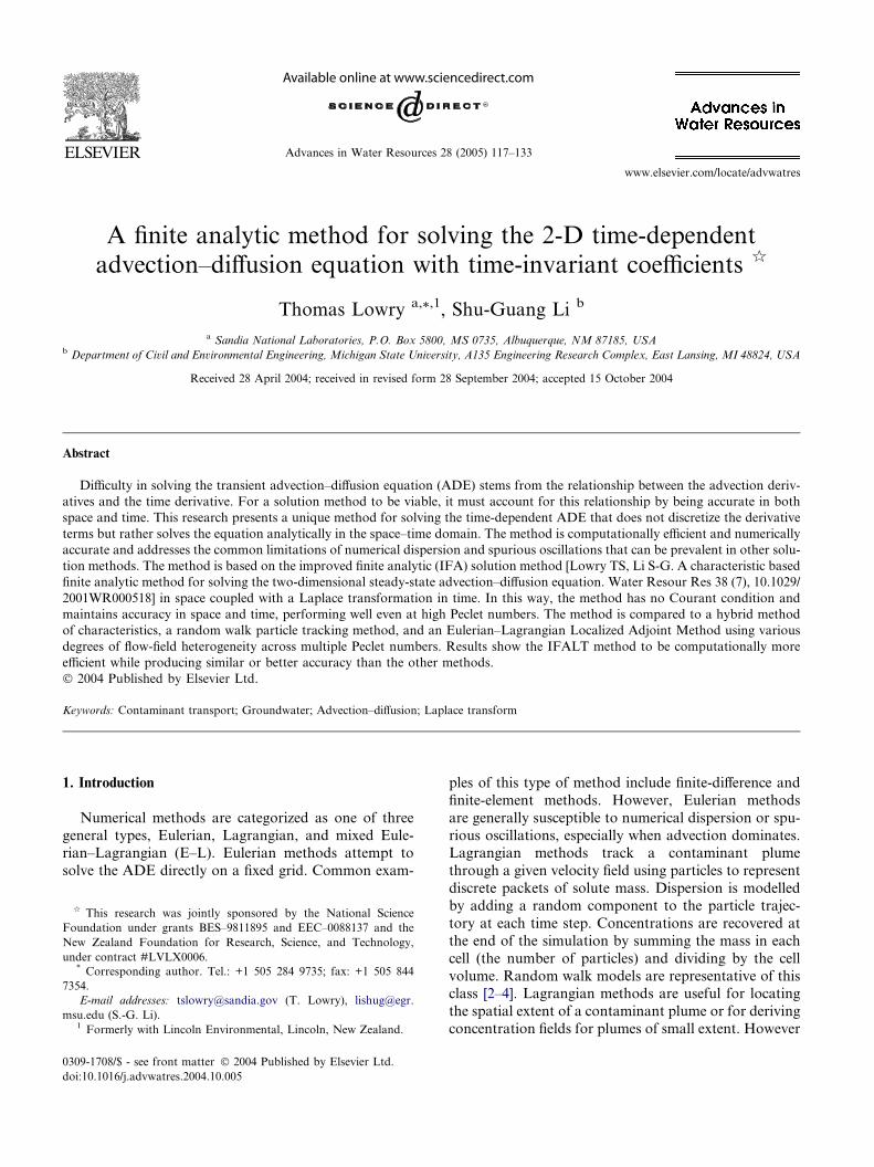
Figs. 6–11 show the two-dimensional plumes for 2a

to 2f, respectively.

3.3. Example 3—deterministic flow field

Example 3 simulates advective transport of a Gaus-

sian plume through a deterministic, sinusoidal velocity

field. The equations describing the velocities in the x

and y directions are

V x ¼ U const ð21Þ

and

V y ¼ V mag sinpxP

� �þ V const ð22Þ

where Vx is the velocity in the x-direction which is equal

to a constant velocity Uconst, Vy is the velocity in the

y-direction, Vmag is the velocity amplitude, x is the x-

position in the domain, P is the half period of the sinefunction, and Vconst is a constant.

This example simulates two mean directions of flow,

one at 22.5� above horizontal and the other at 45.0�.These examples are labelled as 3a (22.5�) and 3b

(45.0�). By adding the sine function to the constant

y-velocity, the plume deforms and then reforms every

P units in the x-direction (Fig. 12). By not simulating

dispersion and molecular diffusion, we can comparethe plume every nP units in the x-direction from the

starting point directly to the initial condition to assess

each methods ability to handle complicated flow regimes

that are not oriented with the grid. The significance of

Example 3a is that the 22.5� angle represents the worst

case scenario for the IFALT method since that is the an-

gle where the interpolation distance along each cell

boundary is the highest.

Both 3a and 3b use a uniform domain that is 275

cells in the x-direction and 275 cells in the y-directionwith each cell measuring 1m by 1m. For Example

3a, the flow field is described by setting

Uconst = 1.0m/d, Vmag = 2.0m/d, P = 15m, and

Vconst = 0.4142m/d. Example 3b changes Vconst to

1m/d. The simulation time for both Examples is 180

days, which means the plume deforms and reforms

15 times during its migration (Fig. 12). Run-time

parameters for this example are shown in Table 8. Re-sults are presented by transecting the plume parallel to

the y-axis through its center, and plotting the dimen-

sionless concentration along that line. These plots are

shown in Figs. 13 and 14. Additionally, run-times

and mass-balance for both methods are compared

and shown in Table 9.

Fig. 7. Concentration contours for Example 2b. The number in the

lower left hand corner is the simulation runtime in h:m:s format.Fig. 8. Concentration contours for Example 2c. The number in the



4. Discussion

For Example 1a, the IFALT and HMOC methods

were able to match the analytical solution almost ex-

actly. The ELLAM method suffered from non-physical

oscillations at the solute interface and the FDLT suf-

fered from severe numerical dispersion. With the added

dispersion (1b and 1c), the IFALT and ELLAM meth-

ods matched the analytical solution while the HMOCmethod showed spikes in the break through curve due

to the particle nature of the solution. The oscillations

present in the ELLAM simulation were not present for

the cases with dispersion. The IFALT method was able

to closely match the analytical solution in all cases.

For the simulations in Example 2, all methods

matched the overall shape and character of each plume

(Figs. 6–11). Generally, as the degree of heterogeneity

increased, and the level of dispersion decreased, the

matches deteriorated, mainly due to numerical disper-

sion and/or spurious oscillations. This is evident by

examining the maximum and minimum dimensionless

concentrations (C/C0) for each simulation (Table 7).

The best matches occurred for simulation 2c, wherethe IFALT method showed a maximum dimensionless

concentration (MDC) of 0.62, as compared to 0.64 for

the HMOC method, 0.69 for the ELLAM method,

and 1.19 for the RW method. The high-resolution ‘‘ex-

act’’ solution returned a MDC of 0.61. Negative concen-

trations were predicted by both the IFALT and

ELLAM methods across all simulations due to oscilla-

tions from the Laplace inverse routine and from spuri-ous oscillations, respectively. The ELLAM method

also showed MDC�s much higher than the ‘‘exact’’ solu-

tion for simulations 2a–c.

Fig. 9. Concentration contours for Example 2d. The number in the


Fig. 10. Concentration contours for Example 2e. The number in the



The HMOC and RW methods were the most com-

putationally costly while the IFALT method was the

least costly. Not including the high-resolution HMOC

simulation (which had run times on the order of five

days), run times across all of Example 2 ranged from

just over 4h for the RW simulation in 2f to 1.2m for

the IFALT method in 2a. The IFALT method provided

the best balance of accuracy and efficiency, offering anapproximate order of magnitude decrease in simulation

time over the ELLAM method, and approximately two-

orders magnitude over the HMOC and RW methods.

Across all runs of Example 2, the IFALT method was

3.23 (2f) to 6.00 (2a) times faster then the ELLAM

method, 6.61 (2c) to 39.42 (2d) times faster than the

HMOC method, and 26.81 (2c) to 111.79 (2d) times fas-

ter then the RW method.

The third example compares only the ELLAM and

IFALT methods and shows the IFALT method provid-

ing virtually identical results to the ELLAM method.

For Example 3a, the cross-section plots overlay the ana-

lytical solution almost exactly, with the mass balance

providing 99.99% and 99.989% for the ELLAM and

IFALT methods, respectively. For Example 3b, themass balance is 99.99% and 99.989% (ELLAM and

IFALT). Computationally the IFALT method was fas-

ter, with a simulation time of 1min 36.54s for Example

3a as compared to 2min, 44.53s for the ELLAM meth-

od. For Example 3b the times were 1min, 34.14s and

3min, 1.72s for the IFALT and ELLAM methods,

respectively.

The efficiency of the IFALT method over the time-stepping methods will increase as the simulated time in-

creases since the computational run time for the IFALT

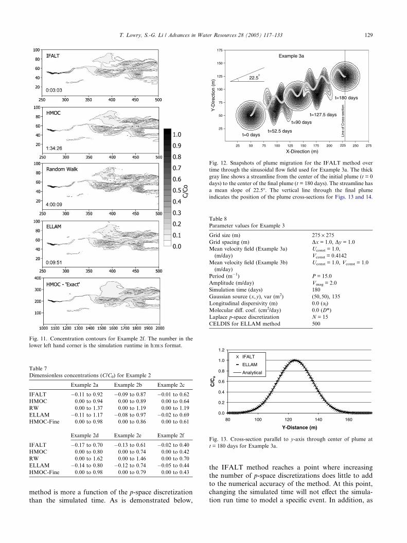
Fig. 11. Concentration contours for Example 2f. The number in the


25 50 75 100 125 150 175 200 250 275

25

50

75

100

125

150

175

X-Direction (m)

Y-D

irect

ion

(m)

t=0 dayst=52.5 days

t=90 days

t=127.5 days

Example 3a

22.5

Line

of C

ross

-sec

tion

t=180 days

225

Fig. 12. Snapshots of plume migration for the IFALT method over

time through the sinusoidal flow field used for Example 3a. The thick

gray line shows a streamline from the center of the initial plume (t = 0

days) to the center of the final plume (t = 180 days). The streamline has

a mean slope of 22.5�. The vertical line through the final plume

indicates the position of the plume cross-sections for Figs. 13 and 14.

Table 7

Dimensionless concentrations (C/C0) for Example 2

Example 2a Example 2b Example 2c

IFALT �0.11 to 0.92 �0.09 to 0.87 �0.01 to 0.62

HMOC 0.00 to 0.94 0.00 to 0.89 0.00 to 0.64

RW 0.00 to 1.37 0.00 to 1.19 0.00 to 1.19

ELLAM �0.11 to 1.17 �0.08 to 0.97 �0.02 to 0.69

HMOC-Fine 0.00 to 0.98 0.00 to 0.86 0.00 to 0.61

Example 2d Example 2e Example 2f

IFALT �0.17 to 0.70 �0.13 to 0.61 �0.02 to 0.40

HMOC 0.00 to 0.80 0.00 to 0.74 0.00 to 0.42

RW 0.00 to 1.62 0.00 to 1.46 0.00 to 0.70

ELLAM �0.14 to 0.80 �0.12 to 0.74 �0.05 to 0.44

HMOC-Fine 0.00 to 0.98 0.00 to 0.79 0.00 to 0.43

Table 8


Grid size (m) 275 · 275


Mean velocity field (Example 3a)

(m/day)

Uconst = 1.0,

Vconst = 0.4142

Mean velocity field (Example 3b)

(m/day)

Uconst = 1.0, Vconst = 1.0

Period (m�1) P = 15.0

Amplitude (m/day) Vmag = 2.0


Gaussian source (x,y), var (m2) (50,50), 135

Longitudinal dispersivity (m) 0.0 (al)Molecular diff. coef. (cm2/day) 0.0 (D*)

Laplace p-space discretization N = 15

CELDIS for ELLAM method 500

0.0

0.2

0.4

0.6

0.8

1.0

1.2

80 100 120 140 160

Y-Distance (m)

C/C

o

IFALT

ELLAM

Analytical

Fig. 13. Cross-section parallel to y-axis through center of plume at

t = 180 days for Example 3a.


method is more a function of the p-space discretization

than the simulated time. As is demonstrated below,

the IFALT method reaches a point where increasing

the number of p-space discretizations does little to add

to the numerical accuracy of the method. At this point,

changing the simulated time will not effect the simula-

tion run time to model a specific event. In addition, as

Table 9

Run times and mass balance for Example 3

Solution

method

3a Run

time (s)

3a Mass

balance

3b Run

time (s)

3b Mass

balance

IFALT 96.5 99.894% 94.1 99.800%

ELLAM 164.5 99.996% 181.7 99.992%

0.0

0.2

0.4

0.6

0.8

1.0

1.2

180 200 220 240 260

Y-Distance (m)

C/C

o

IFALT

ELLAM

Analytical

Fig. 14. Cross-section parallel to y-axis through center of plume at

t = 180 days for Example 3b.

0.80

0.85

0.90

0.95

1.00

1.05

1.10

1.15

1.20

173 174 175 176 177 178 179 180 181 182Distance (m)

C/C

o

130

75

50

30

5

Analytical

# of Laplace p Evaluations

Fig. 15. Each line shows the IFALT solution as obtained using the

indicated number of Laplace p evaluations. Generally as the number of

evaluations goes up, oscillations diminish and accuracy increases.

0.80

0.85

0.90

0.95

1.00

1.05

1.10

1.15

1.20

173 174 175 176 177 178 179 180 181 182

Distance (m)

C/C

0

dx = dy = 0.5 m

dx = dy = 2.5 m

dx = dy = 5.0 m

Analytical

dx = dy = 1.0 m

Fig. 16. As the grid size increases, oscillations associated with the

Laplace transform inverse routine are reduced.


the degree of heterogeneity increases, the time-stepping

methods are forced towards smaller time steps and

longer computational run times, which again increases

the relative efficiency of the IFALT method over the

other methods. The implications of this speed improve-

ment are significant, especially if one considers the

improved ability to perform sensitivity or Monte Carlo

analysis or model set-up and calibration.Outside the increase in simulation efficiency, the

IFALT method has the added benefit of performing

the inversion at any time less then the maximum simula-

tion time. If at a later time, the need arises to examine

results that are different from your initial output, you

simply run the inversion program at the new time with-

out having to re-run the entire model.

4.1. Sensitivity to temporal and spatial discretization

To test the IFALT method�s robustness and accuracy

over different grid sizes and p-space discretizations, we

use the same spatial extent and source configuration as

Example 1a, but use grid spacings of 0.5m, 1.0m,

2.5m, and 5m coupled with p-space discretizations of

N = 5, 30, 50, 75, and 130.Fig. 15 shows a close-up of the upper trailing edge of

the solute step-function, using the base-case grid size of

1m square, and varying the number of p-space discreti-

zations. For N = 5, the solution is highly oscillatory and

quite unsatisfactory. However as N increases, the oscil-

lations diminish. At N = 50, there is a slight rounding

of the sharp edge and for NP 75, the solution matches

the analytical solution almost exactly.

The same trend can be seen if the p-space discretiza-

tions are held constant and the grid spacing is varied.

Fig. 16 again shows a close up of the trailing edge of

the step-function, but with a fixed value of N = 30 and

the grid spacing varying as described above. Generally,as the grid space is increased, the oscillations diminish.

This is what is predicted by Eq. (19). However, as with

any solution method, if the spacing becomes too large

(e.g. when Dx = Dy = 5.0m) the quality of the solution

diminishes due to a loss of resolution.

As another example, Fig. 17 shows the natural log of

the root mean square error (RMSE) and the simulation

run time as compared to the number of p-space discret-izations for simulations based on Example 3a. The

RMSE is calculated by the following equation:

RMSE ¼

ffiffiffiffiffiffiffiffiffiffiffiffiffiffiffiffiffiffiffiffiffiffiffiffiffiffiffiffiffiffiffiffiffiffiffiffiffiffiffiffiffiffiffiffiffiPNxi¼1

PNy

j¼1ðCi;j � Cai;jÞ

2

Nx � Ny

sð23Þ

where Ci,j is the concentration as predicted by the model

in cell i, j, Cai;j is the analytical solution in cell i, j, Nx is

the number of cells in the x-direction, and Ny is the

number of cells in the y-direction. As can be seen in

0

20

40

60

80

100

120

140

160

0 5 10 15 20 25

P-Space Iterations (N)

Ru

n T

ime

(sec

)

-7.0

-6.0

-5.0

-4.0

-3.0

-2.0

-1.0

0.0

Ln

(RM

SE

)

Run Time

Ln(RMSE)

Fig. 17. Run time and natural log of RMSE versus the number of p-

space iterations.

0

20

40

60

80

100

120

0 20 40 60 80 100 120 140 160 180 200

Simulated Time (days)

Run

Tim

e (s

ecs)

-6.55

-6.50

-6.45

-6.40

-6.35

-6.30

-6.25

-6.20

-6.15

Ln(R

MS

E)

Run Time

Ln(RMSE)

Fig. 18. Run time and natural log of RMSE versus simulated time.


Fig. 17, the simulation run time is a linear function ofthe p-space discretization. This is evident when one

examines Eqs. (8) and (15), which shows both the solu-

tion and the Laplace inversion as linear combinations of

p. It is also evident that increasing the p-space discretiza-

tion beyond a certain point quickly reaches a point of

diminishing returns, and illustrates why a value of

N = 15 was used for Example 3a.

Similarly, Fig. 18 shows the natural log of the RMSEand the simulation run time as compared to the simu-

lated time for simulations based on Example 3a. As

the simulated time increases, the solution accuracy gen-

erally decreases, although looking at the range of

RMSE, the differences are minimal. Likewise, the simu-

lation run time also increases with the simulated time.

This is because the code only calculates concentration

in a cell if the upwind cells reach a user-defined concen-tration threshold. As the plume trajectory fills a higher

percentage of the grid, more cells are involved in the cal-

culation, which increases the computational effort. For

simulations where no cells are left uncalculated, increas-

ing the simulated time does not increase the simulation

run time.

5. Summary and conclusions

In this paper, we have developed an improved finite

analytic Laplace transform method (IFALT) for solving

the transient advection–dispersion equation in advection

dominated, time-invariant, heterogeneous flow fields.

The method starts by applying a Laplace transform to

the transient advection diffusion equation, which pro-

duces a ‘‘steady-state’’ (in form) equation that describes

the spatial variation of the concentration in complex La-

place space. The steady-state transformed equation is

solved using an improved finite analytic (IFA) method[1,11,52] and then transformed back to the real space–

time domain using an efficient Laplace inverse routine

[34]. The uniqueness of this work lies in the fact that it

produces a time continuous solution method that is

accurate in both space and time.

The solution is evaluated once for each Laplace p va-

lue (usually on the order of 10–50 times) and then in-

verted back to the real space–time domain at somefuture time. This means the IFALT method is much

more efficient than time-stepping methods in that there

are no Courant conditions. Comparisons to a random

walk particle tracking method, an Eulerian–Lagrangian

localized adjoint method, and a hybrid method of char-

acteristics show the IFALT method provides similar or

better accuracy for the same problem but with computa-

tional run times on the order of 3–100 times less. Thisincrease in efficiency has large implications with regards

to sensitivity and/or Monte Carlo analysis or anytime

statistical evaluation is necessary.

Improvements of the efficiency of the IFALT method

are still possible by replacing the inefficient SOR itera-

tive solver used here, with a faster more efficient sparse

matrix solver. Indications are this type of change may

result in an additional speed increase of 2–5 times overthe SOR solver, especially in cases of modelled disper-

sion. Another attractive feature of the Laplace trans-

form technique is that each Laplace p space solution is

independent, making the IFALT method well suited

for parallel processing. Lastly the method outlined in

this work lends itself to three-dimensional and dual

porosity transport as well. While the application to

three-dimensions is similar to the two-dimensional caseand relatively straight forward, the logic in the program-

ming and implementation is difficult. Work on this

problem is underway with significant progress to date.

References

[1] Lowry TS, Li S-G. A characteristic based finite analytic method for

solving the two-dimensional steady-state advection–diffusion equa-

tion. Water Resour Res 2001; 38 (7) [10.1029/2001WR000518].

[2] Uffink G. A random walk model for the simulation of macrodis-

persion in a stratified aquifer. IAHS Publ 1985;146:103–14.

[3] Kinzelbach W. The random walk method in pollutant transport

simulation. Groundwater Flow Quality Modell 1988:227–46.

[4] Tompson AF, Gelhar LW. Numerical simulation of solute

transport in three-dimensional randomly heterogeneous porus

media. Water Resour Res 1990;26(10):2541–62.

[5] Al-Lawatia M, Sharpley RC, Wang H. Second-order character-

istic methods; for advection diffusion equations and comparison

to other scehmes. Adv Water Res 1999;22(7):741–68.


[6] Russell T. Eulerian–Lagrangian localized adjoint methods for

advection-dominated problems, Numerical Analysis 1989. Pitman

Res Notes Math Ser 1989;228:206–28.

[7] Celia M, Russell T, Herrera I, Ewing R. An Eulerian–Lagrangian

localized adjoint method for the advection diffusion equation.

Adv Water Res 1990;13(4):187–206.

[8] Healy R, Russell T. A finite-volume Eulerian–Lagrangian local-

ized adjoint method for solution of the advection–dispersion

equation. Water Resour Res 1993;29(7):2399–413.

[9] Ruan F, Dennis M. An investigation of Eulerian–Lagrangian

methods for solving heterogeneous advection-dominated trans-

port problems. Water Resour Res 1999;35(8):2359–73.

[10] Chen C, Chen H. Finite-analytic numerical method for unsteady

two-dimensional Navier–Stokes equations. J Comput Phys

1984;52:209–26.

[11] Li S-G, Wei SC. Improved finite-analytic methods for steady-state

heterogeneous transport in multi-dimensions. J Hydraul Eng

1998;124(4):358.

[12] C. Chen, P. Li, Finite differential method in heat conduction–

application of analytic solution technique. ASME Paper 79-WA/

HT-50, 1979, p. 250, 2–7 December, ASME Winter Annual

Meeting, New York, NY, 1979.

[13] Chen C, Naseri-Neshat H, Ho K. Finite-analytic numerical

solution of heat transfer in two-dimensional cavity flow. J Numer

Heat Transfer 1981;4:179–97.

[14] Chwang A, Chen H. Optimal finite difference method for potential

flows. J Eng Mech 1987;113(11):1759–73.

[15] Chen C, Yoon Y. Finite-analytic numerical solution of axisym-

metric Navier–Stokes and energy equations. J Heat Transfer

1983;105:639–45.

[16] Choi S, Chen C. Finite analytic numerical solution of turbulent

flow past axisymmetric bodies by zone modeling approach.

ASME, Fluids Eng Div FED 1985;66:23–32.

[17] Elnawawy O, Valocchi A, Ougouag A. The cell analytical-

numerical method for solution of advection–dispersion equation:

two-dimensional problems. Water Resour Res 1990;6(11):

2705–16.

[18] Hwang JC, Chen C-J, Sheikoslami M, Panigrahi BK. Finite-

analytic numerical solutions for two dimensional groundwater

solute transport. Water Resour Res 1985;21(9):1354–60.

[19] Chen C, Chen H, Finite analytic numerical method for unsteady

two-dimensional Navier–Stokes equations. Tech rep, Energy

Division and Iowa Institute of Hydraulic Research, University

of Iowa, Iowa City, IA, December 1982.

[20] Tsai W-F, Tien H-C, Chen C-J. Finite analytic numerical

solutions for unsaturated flow with irregular boundaries. J

Hydraul Eng 1993;119(11):1274–97.

[21] Wang C. Characteristic finite analytic method (CFAM) for

incompressible Navier–Stokes equations. Acta Mech

2000;143:57–66.

[22] Li S-G, Ruan F, McLaughlin D. A space–time accurate method

for solving solute transport problems. Water Resour Res

1992;28(9):2297–306.

[23] Gurtin M. Variational principles for linear initial value problems.

Q Appl Math 1965;22:252–6.

[24] Javandel I, Witherspoon P. Application of the finite element

method to transient flow in porous media. Soc Pet Eng J

1968;8:241–52.

[25] Liggett J, Liu P-F. The boundary integral equation method for

porous media flow, Winchester, Mass, 1983.

[26] Moridis G, Reddell R. The Laplace transform finite difference

method for simulation of flow through porous media. Water

Resour Res 1991;27(8):1873–84.

[27] Sudicky E. The Laplace transform Galerkin technique: a

time-continuous finite element theory and application to

mass transport in groundwater. Water Resour Res 1989;25(8):

1833–46.

[28] Sudicky E. The Laplace transform Galerkin technique for efficient

time-continuous solution of solute transport in double-porosity

media. Geoderma 1990;46:209–32.

[29] Sudicky E, McLaren R. The Laplace transform Galerkin

technique for large-scale simulation of mass transport in discretely

fractured porous formations. Water Resour Res 1992;28(2):

499–514.

[30] Ren L. A hybrid Laplace transform finite element method for

solute radial dispersion problem in subsurface flow. J Hydrody-

nam 1994;9:37–43.

[31] Ren L, Zhang R. Hybrid Laplace transform finite element method

for solving the convection–dispersion problem. Adv Water Res

1999;23:229–37.

[32] Carrier G. Partial differential equations. San Diego, CA: Aca-

demic Press, Inc; 1976.

[33] Holly F, Preissmann A. Accurate calculation of transport in two

dimensions. J Hydraul Div Am Soc Civ Eng 1977;103(HY11):

1259–77.

[34] DeHoog F, Knight J, Stokes A. An improved method for

numerical inversion of Laplace transforms. SIAM J Sci Stat

Comput 1982;3(3):357–66.

[35] Dubner H, Abate J. Numerical inversion of Laplace transforms

by relating them to the finite Fourier cosine transform. J Assoc

Comput Mach 1968;15(1):115–23.

[36] Cooley J, Lewis P, Welch P. The fast Fourier transform

algorithm: Programming considerations in the calculation of

sine, cosine, and Laplace transforms. J Sound Vib 1970;12:

315–37.

[37] Crump KS. Numerical inversion of Laplace transforms using a

Fourier series approximation. J Assoc Comput Mach 1976;23(1):

89–96.

[38] Durbin F. Numerical inversion of Laplace transforms: an efficient

improvement to Dubner and Abate�s method. Comput J

1974;17:371–6.

[39] Silverberg M. Improving the efficiency of Laplace-transform

inversion for network analysis. Electron Lett 1970;6:105–6.

[40] Zheng C. MT3D A modular three-dimensional transport

model for simulation of advection, dispersion, and chemical

reactions of contaminants in groundwater systems. In: Docu-

mentation and users guide. S.S. Papadopulos & Associates;

1991–92.

[41] Zheng C, Wang P. Mt3dms: a modular three-dimensional

multispecies model for simulation of advection, dispersion, and

chemical reactions of contaminants in groundwater systems.

Documentation and users guide. Tech rep, US Army Engineer

Research and Development Center, Vicksburg, MS, 1999.

[42] Wang H, Russell TF, Ewing RE. Eulerian–Lagrangian localized

adjoint methods for variable-coefficient convection–diffusion

problems arising in groundwater applications. Numer Methods

Water Resour 1992:25–31.

[43] Celia M. Eulerian–Lagrangian localized adjoint methods for

contaminant transport simulations. In: Peters A, editor. Proceed-

ings of the 10th International Conference on Computation

Methods in Water Resources. Dordrecht: Kluwer; 1994.

[44] Konikow L, Goode D. Hornberger G. A three-dimensional

method of characteristics solute transport model (MOC3D). Tech

Rep 96–4267, US Geological Survey, Reston, VA.

[45] Heberton C, Russell T, Konikow L, Hornberger G. A three

dimensional finite volume Eulerian–Lagrangian localized adjoint

method (ELLAM) for solute-transport modeling, Tech Rep 00-

4087, US Geological Survey, Reston, VA.

[46] M. Al-Lawatia, H. Wang, A preliminary investigation on an

ELLAM scheme for linear transport equations. Numer. Methods

Partial Differ Equat 2002;19 (1), doi:10.1002/num.10042.

[47] Russell TF, Celia MA. An overview of research on Eulerian–

Lagrangian localized adjoint methods (ELLAM). Adv Water Res

2002;25:1215–31.

http://dx.doi.org/10.1002/num.10042


[48] T. Prickett, T. Naymik, C. Lonnquist, A �random walk� solutetransportmodel for selected groundwater quality evaluations. Tech

Rep Bull 65, Illinois State Water Survey, Champaign, IL, 1981.

[49] Runkel RL. Solution to the advection–dispersion equation:

Continuous load of finite duration. USGS Otis Documentation

Web Publication, 1996. Available from: <http://webserver.cr.

usgs.gov/otis/documentation/r96/r96.html>.

[50] Burr D, Sudicky E, Naff R. Nonreactive and reactive solute

transport in three-dimensional heterogeneous porous media:

Mean displacement, plume spreading, and uncertainty. Water

Resour Res 1994;30(3):791–815.

[51] Sudicky E. A natural gradient experiment on solute transport in a

sand aquifer: spatial variability of hydraulic conductivity and its

role in the dispersion process. Water Resour Res 1986;22(15):

2069–82.

[52] Lowry TS. An improved finite analytic method for unsteady

transport in heterogeneous porous media. PhD thesis, Portland

State University, 2000.

http://webserver.cr.usgs.gov/otis/documentation/r96/r96.html

http://webserver.cr.usgs.gov/otis/documentation/r96/r96.html

A ﬁnite analytic method for solving the 2-D...

Documents

Transcript of A ﬁnite analytic method for solving the 2-D...