A NEWTON-PICARD APPROACH FOREFFICIENT NUMERICAL SOLUTION OF TIME-PERIODIC

PARABOLIC PDE CONSTRAINED OPTIMIZATION PROBLEMS

A. POTSCHKA∗† , M.S. MOMMER† , J.P. SCHLODER† , AND H.G. BOCK∗†

Abstract. We investigate an iterative method for the solution of time-periodic parabolic PDEconstrained optimization problems. It is an inexact Sequential Quadratic Programming (iSQP)method based on the Newton-Picard approach. We present and analyze a linear quadratic modelproblem and prove optimal mesh-independent convergence rates. Additionally, we propose a two-gridvariant of the Newton-Picard method. Numerical results for the classical and the two-grid variantsof the Newton-Picard iSQP method as a solver and as a preconditioner for GMRES are presented.

Key words. optimal control, periodic boundary condition, parabolic PDE, Newton-Picard,simultaneous optimization, inexact SQP, Krylov method preconditioner

AMS subject classifications. 35K20, 65F08, 65F10, 65K05, 65N55

1. Introduction. Let Ω ⊂ Rd be a bounded open domain with Lipschitz bound-ary ∂Ω and let Σ := (0, 1) × ∂Ω. We look for controls u ∈ L2(Σ) and correspondingstates y ∈ W (0, 1) = y ∈ L2(0, 1;H1(Ω)) : yt ∈ L2(0, 1;H1(Ω)∗) which solve thetime-periodic PDE constrained optimization problem

minimizeu∈L2(Σ),y∈W (0,1)

J(y(1; .), u) :=12

∫Ω

(y(1; .)− y)2 +γ

2

∫∫Σ

u2 (1.1a)

subject to yt = D∆y, in (0, 1)× Ω, (1.1b)yν + βy = αu, in (0, 1)× ∂Ω, (1.1c)y(0; .) = y(1; .), in Ω, (1.1d)

with α, β ∈ L∞(∂Ω) non-zero and positive a.e., and D, γ > 0.The work of Barbu [2] considers a similar problem with a more general formula-

tion of the underlying linear parabolic PDE in a Hilbert-space valued ODE setting.However, existence and uniqueness results do not carry over to problem (1.1) becauseof the different choice of objective function which excludes the case of point evalu-ations of the state y at time t = 1. An analysis for periodic optimal control of theBoussinesq equation can be found in Trenchea [15].

Besides analytical results, we are interested in efficient numerical methods forproblem (1.1) and their analysis. Most of the work on numerical methods for theseproblems can be found in the more application oriented literature which we shalldescribe in the following. For instance, many processes in chemical engineering areoperated in a periodic manner, e.g., separation processes like Simulated Moving Bed(SMB) or Pressure Swing Adsorption (PSA), or reaction processes like the ReverseFlow Reactor. The models consist of partial differential equations of parabolic type.

For the efficient simulation of periodic steady states it is important to exploitthe inherent dynamics of dissipative processes, which are characterized by relativelylow-dimensional dynamics even for problems with a high number of variables after

∗This work was supported by the German Research Foundation (DFG) within the priority pro-gram SPP1253 under grant BO864/12-1 and by the German Federal Ministry of Education andResearch (BMBF) under grant 03BONCHD.†Interdisciplinary Center for Scientific Computing, Im Neuenheimer Feld 368, 69123 Heidelberg,

GERMANY. Corresponding authors: (potschka|mario.mommer)@iwr.uni-heidelberg.de

1

discretization. One typical example is the Newton-Picard method proposed by Lustet al. [9].

Numerical optimization of periodic processes is currently an active field of re-search. General purpose structure-exploiting direct optimal control techniques havebeen employed to optimize the SMB process [8, 14] and the PSA process [10]. In allthese works, however, the inherent system dynamics were not exploited in the numer-ical computations. In van Noorden et al. [17], the Newton-Picard method is used tooptimize periodic processes exploiting the inherent dynamics, however, the employedprojected gradient descent method is used in a sequential mode, i.e., after each updateof the control and design parameters the periodic steady state must be calculated tohigh accuracy, which makes the overall algorithm computationally expensive. It wasshown by Bock et al. [3], Hazra et al. [6] that for similar problems in shape optimiza-tion for fluid dynamics a simultaneous method can save up to 70 percent of CPU time.The similarity between the problems is that an efficient iterative method (a solver)is available for the constraint of the optimization problem given control and designparameters. The savings can be gained from performing only one (or few) steps ofthe solver for each step of the optimization algorithm.

One purpose of this article is to investigate a simultaneous optimization algorithmon problem (1.1). The model problem is an extension of the parabolic optimal controlproblem presented, e.g., in the textbook of Troltzsch [16]. The algorithm is basedon the Newton-Picard method and thus exploits the inherent system dynamics. Theresulting method belongs to the class of inexact Sequential Quadratic Programming(iSQP) methods (see, e.g., Griewank and Walther [5]). Preliminary numerical resultsof the Newton-Picard iSQP method for the non-linear SMB process are availablein Potschka et al. [11]. We also present a variant of the Newton-Picard method, whichrelies on a two-grid approach. Multigrid approaches for parabolic optimal controlproblems have been studied by, e.g., Borzı [4]. Recently, Agarwal et al. [1] presenteda reduced order model approach for the optimization of PSA, where a surrogate modelbased on Proper Orthogonal Decomposition (POD) is used in the optimization. Wepersue a different approach, where the reduced order model (generated by the Newton-Picard method) is only used for the generation of derivatives while still using theresiduals of the full model.

The article is organized as follows: In Section 2.1 we establish the existence anduniqueness of the optimal solution of the model problem (1.1). We discuss the opti-mality conditions for the model problem in a Hilbert space setting in Section 2.2 andinvestigate the regularity of the Lagrange multipliers in Section 2.3. In Section 3 wereview the Newton-Picard method in a general setting of Newton-type methods inBanach space. We continue with a presentation of the Newton-Picard iSQP methodfor the model problem in Section 4. In Section 5 we discuss the discretization of theoptimal control problem. In Section 6 we present the Newton-Picard iSQP method forthe discretized problem in the case of a classical Newton-Picard projective approxi-mation and of a coarse-grid approach for the constraint Jacobians. The importance ofthe choice of the scalar product for the projection is highlighted, a question that hasso far not been addressed. We establish an optimal, mesh-independent convergenceresult for the Newton-Picard iSQP method with classical projective approximationand discuss its property of bounded retardation. We also outline the fast solution ofthe subproblems in this section. In Section 7 we present numerical results for differentsets of problem parameters for the Newton-Picard iSQP method as such and as a pre-conditioner for GMRES. In Section 8 we give an outlook on how the Newton-Picard

2

iSQP method can be employed for non-linear optimization problems.

2. On solutions of the model problem.

2.1. Existence and uniqueness of the optimal solution. To show existenceand uniqueness of the solution of problem (1.1), we use the approach persued inTroltzsch [16]: We first prove existence of a linear, continuous “solution operator” Sthat maps a given control u to a solution y of the constraint system (1.1b)–(1.1d).Then we invoke the following theorem that can be found in Troltzsch [16], Satz 2.14–2.17.

Theorem 2.1 (Existence and uniqueness). Let real Hilbert spaces U, ‖.‖U andH, ‖.‖H, y ∈ H, and γ > 0 be given. Suppose further that S : U → H is a linear,continuous operator. Then, the Hilbert space optimization problem

minimizeu∈U

12‖Su− y‖2H +

γ

2‖u‖2U

has a unique solution.We shall now construct the solution operator S : L2(Σ)→ H1(Ω) in three steps.Lemma 2.2. Let a pair of initial state and control (y(0; .), u) ∈ L2(Ω)×L2(Σ) be

given. Then, there exists a unique solution y ∈W (0, 1) to equations (1.1b)–(1.1c) andthere exists a linear, continuous operator S : L2(Ω) × L2(Σ) → H1(Ω) which maps(y(0; .), u) to the final state y(1; .).

Proof. According to, e.g., Wloka [18], equations (1.1b)–(1.1c) have a uniquesolution y ∈W (0, 1) for given y(0; .) ∈ L2(Ω) and u ∈ L2(Σ) and the solution operatorSW : (y(0; .), u) 7→ y is a linear and continuous operator. Furthermore, y can bemodified on a set of measure zero such that y ∈ C(0, 1;H1(Ω)). Thus, the traceoperator T : y 7→ y(1; .) exists and is linear and continuous. Therefore, also theoperator S := TSW is linear and continuous.

In the second step we show contractivity of S(., 0) in H1(Ω). For ease of presen-tation, define the linear, continuous operators G1 : L2(Ω)→ L2(Ω) and G2 : L2(Σ)→L2(Ω) via

G1 := S(., 0) and G2 := S(0, .). (2.1)

Lemma 2.3 (Contractivity). There exists κ < 1 such that for all v ∈ H1(Ω)

‖G1v‖H1(Ω) ≤ κ‖v‖H1(Ω).

Proof. We start by investigating the spatial derivative terms of (1.1b)–(1.1c)with homogeneous Robin boundary condition (i.e., u = 0). They can be expressed invariational form as a symmetric bilinear form a : H1(Ω)×H1(Ω)→ R

a(ϕ, v) := −D∫

Ω

ϕ∆v

= D

∫Ω

∇ϕ · ∇v −D∫∂Ω

ϕ(ν · ∇v) = D

∫Ω

∇ϕ · ∇v +D

∫∂Ω

βϕv.

We define the operator A : H1(Ω)→ H1(Ω) via

〈ϕ,Av〉H1(Ω) := a(ϕ, v) = D

∫Ω

∇ϕ · ∇v +D

∫∂Ω

βϕv. (2.2)

3

The operator A is self-adjoint, its spectrum is real, and A has a set of orthogonaleigenvectors ϕi which form a basis of H1(Ω) (see, e.g., Renardy and Rogers [12]).Furthermore, A is coercive (see Troltzsch [16], equation 2.17), i.e., there exists aconstant ω > 0 such that for all v ∈ H1(Ω)

〈v,Av〉H1(Ω) ≥ ω‖v‖2H1(Ω).

For v = ϕi we obtain the lower bound λi ≥ ω > 0 for the eigenvalue λi. Thus, theLumer-Phillips theorem (cf. Renardy and Rogers [12], Theorem 11.22) yields that theoperator A generates a strongly continuous semigroup exp(−tA) which satisfies theinequality

‖exp(−tA)‖H1(Ω) ≤ exp(−ωt).

Because y(t; .) = exp(−tA)y(0; .) is another representation of the unique solution ofequations (1.1b)–(1.1c) with u = 0, we finally obtain

‖G1v‖H1(Ω) = ‖S(v, 0)‖H1(Ω) = ‖exp(−A)v‖H1(Ω) ≤ exp(−ω)‖v‖H1(Ω) = κ‖v‖H1(Ω),

with κ := exp(−ω) < 1.Remark 2.4. G1 = exp(−A) = exp(−A∗) = exp(−A)∗ = G∗1 is self-adjoint.To finish the proof of existence and uniqueness of the optimal solution, we use a

fixed point argument to show existence and continuity of the solution operator S.Lemma 2.5. Let u ∈ L2(Σ). Then, there exists a unique y0 ∈ H1(Ω) such that

y = S(y0, u) solves the system of constraints (1.1b)–(1.1d). Furthermore, the operatorS : L2(Σ)→ L2(Ω) defined by S(u) := y0 is linear and continuous.

Proof. We seek for a solution y0 of one of the three equivalent equations

G1y0 +G2u− y0 = 0 ⇔ y0 = G1y0 +G2u ⇔ y0 = (I−G1)−1G2u. (2.3)

The middle equation, Lemma 2.3, and the Banach Fixed Point Theorem yield theexistence and uniqueness of y0 ∈ H1(Ω). The eigenvectors ϕi of A defined in equa-tion (2.2) are also eigenvectors of I − G1. Thus, the eigenvalues of I − G1 can bebounded away from zero by 1− κ in modulus. This yields

‖Su‖L2(Ω) ≤ ‖Su‖H1(Ω) = ‖(I−G1)−1G2u‖H1(Ω) ≤‖G2‖H1(Ω)

1− κ‖u‖L2(Σ). (2.4)

Hence, S : L2(Σ)→ L2(Ω) is a linear and continuous operator (even into H1(Ω)).Corollary 2.6. The optimization problem (1.1) has a unique optimal solution.Proof. Lemma 2.5 and Theorem 2.1.

2.2. Optimality conditions. We eliminate constraints (1.1b) and (1.1c) fromproblem (1.1) via S from Lemma 2.2 and use the Lagrange-formalism to derive nec-essary optimality conditions. By convexity they are also sufficient. For notationalconvenience we shall from now on write y instead of y(0; .). Define the LagrangianL : L2(Ω)× L2(Σ)× L2(Ω)→ R via

L(y, u, λ) = J(y, u) + 〈λ, (G1 − I) y +G2u〉L2(Ω). (2.5)

Regarding the chosen spaces for the Lagrangian, we are now looking for states in thelarger space L2(Ω) instead of H1(Ω). This does not introduce additional solutions to

4

the original problem because y ∈ H1(Ω) is ensured via the periodicity constraint (2.1).The optimality condition is then

L′(y, u, λ)(δy, δu, δλ) = 0, ∀δy ∈ L2(Ω), δu ∈ L2(Σ), δλ ∈ L2(Ω).

A simple calculation yields

L′(y, u, λ)(δy, δu, δλ) = 〈y − y, δy〉+ γ〈u, δu〉+ 〈λ, (G1 − I) δy +G2δu〉+ 〈δλ, (G1 − I) y +G2u〉.

Written in block-operator form, we obtain the Karush-Kuhn-Tucker system I 0 G∗1 − I0 γI G∗2

G1 − I G2 0

yuλ

=

y00

. (2.6)

The block-operator on the left-hand side of equation (2.6) shall be denoted by K :L2(Ω)× L2(Σ)× L2(Ω)→ L2(Ω)× L2(Σ)× L2(Ω).

2.3. Regularity of the Lagrange multiplier. We are going to show that theLagrange multiplier of the periodicity constraint inherits higher regularity from thetarget y.

Theorem 2.7. Let the subset E ⊂ Ω be open and λ ∈ L2(Ω) be the optimalLagrange multiplier of problem (1.1). If y

∣∣E∈ H1(E), then λ

∣∣E∈ H1(E).

Proof. Let the optimal state be denoted by y ∈ H1(Ω). From the first line ofKKT system (2.6), we obtain for λ the fixed point equation

λ = G∗1λ− (y − y).

We construct a sequence

λk+1 = G∗1λk − (y − y),

which converges in L2(Ω) due to Remark 2.4 and Lemma 2.3. Let now E ⊂ Ω beopen and such that y

∣∣E∈ H1(Ω). Then, the sequence (λk

∣∣E

) converges in H1(E).Thus, λ

∣∣E∈ H1(E).

3. The Newton-Picard method for general fixed point problems. LetV be a Banach space and Φ : V → V be a possibly non-linear continuously Frechetdifferentiable mapping with derivative Φ′ ∈ L(V, V ). We are interested in finding asolution v ∈ V of the fixed point equation

v = Φ(v). (3.1)

If v ∈ V is a solution of equation (3.1), and if furthermore Φ′(v) has a spectral radiusof κ < 1, then there exists a neighborhood U of v such that for each v0 ∈ U thesequence (vk) defined by

vk+1 := Φ(vk) (3.2)

converges to v with an asymptotic linear convergence rate of κ.A different way of solving equation (3.1) is to use Newton’s method for finding a

root of the problem

Φ(v)− v = 0. (3.3)5

This leads to the iteration

vk+1 = vk − (Φ′(vk)− I)−1 (Φ(vk)− vk) , (3.4)

which is also known to converge to v in a neighborhood U of v but with quadraticconvergence rate and without the need for contractive Φ′(v). From a computationalpoint of view, the evaluation of the derivative Φ′(vk) and the inversion of Φ′(vk) − Imay be prohibitively expensive. The cost for evaluation and inversion can be reducedby approximating (Φ′(vk)− I)−1 ≈ Jk suitably, resulting in the iteration

vk+1 = vk − Jk (Φ(vk)− vk) . (3.5)

This leads to the class of so-called Newton-type methods, which do not exhibitquadratic local convergence any more. By approximating Φ′(vk) with zero, we seethat the fixed point recurrence (3.2) can also be interpreted as a Newton-type methodwith Jk = −I.

For fixed u, the periodicity equation (2.3) is of the described form with Φ′(vk) =G1. The operator G1 maps the initial state values to the end values of the solution ofthe dynamic system. Thus, the iterate vk of the fixed point iteration (3.2) correspondsto a continuous integration of the system dynamics over k periods. This iteration iscalled Picard method.

It was proposed by Lust et al. [9] to use a low-rank projective approximation ofΦ′(vk). It can be shown that this is equivalent with using Newton’s method on a(hopefully small) subspace of “slow” modes (in the sense of contraction of the fixedpoint iteration (3.2)) and performing pure Picard iteration on the anyway “fast”remaining modes, leading to an overall fast linear convergence with cheap evaluationof Jk.

4. Newton-Picard for optimal control problems: The Newton-Picardinexact Sequential Quadratic Programming method. In this section we in-vestigate how the Newton-Picard method for the forward problem (i.e., solving for aperiodic state for given controls) can be exploited in a so-called “simultaneous opti-mization” approach as opposed to a “sequential optimization” approach.

In the sequential approach, one completely eliminates the states from the op-timization problem, because for each control u the Newton-Picard method yields acorresponding state y(u) which satisfies the periodicity constraint (1.1d). The re-sulting unconstrained problem is solved by standard descent methods, e.g., gradientmethods or variants of Newton’s method, yielding only feasible iterates. The maindrawback of this approach is that a lot of effort (i.e., Newton-Picard iterations) isspent for resolving the system dynamics far away from the solution. The sequentialapproach does not have the property of bounded retardation, i.e., the numerical effortfor solving the constrained optimization problem is not bounded by a small constanttimes the effort spent on solving one forward problem.

The simultaneous approach tries to overcome this disadvantage by performingonly a small number of steps (ideally only one) of the solver for the forward problemper optimization step. The intermediate iterates are not feasible with respect toperiodicity any more, but each iterate is less expensive than in the sequential approach.The simultaneous approach has been used successfully in, e.g., one-shot methods forshape optimization in fluid dynamics [3, 6].

The simultaneous Newton-Picard optimization approach can be written as aninexact Sequential Quadratic Programming (iSQP) method with approximated con-

6

straint derivatives. Let G1 denote the approximation of G1 and regard the approxi-mated KKT system

K :=

I 0 G∗1 − I0 γI G∗2

G1 − I G2 0

.

In the case of pure Picard, G1 = 0 is used. The inexact SQP method generatesiterates via yk+1

uk+1

λk+1

=

ykukλk

− K−1

Kykukλk

−y0

0

. (4.1)

Let ∆K = K −K. The contraction rate is determined by the spectral radius of

K−1∆K =

I 0 G∗1 − I0 γI G∗2

G1 − I G2 0

−1 0 0 ∆G∗10 0 0

∆G1 0 0

,

where ∆G1 = G1 −G1.

5. Discretization of the optimal control problem. First, we discretize thecontrols in space with nu form functions ql whose amplitude can be controlled in time,i.e.,

u(t, x) =nu∑l=1

ul(t)ql(x), ul ∈ L2(0, 1), ql ∈ L2(∂Ω).

We continue with discretizing the initial state y using Finite Elements. Let ϕi denotethe i-th Finite Element basis function and define the following Finite Element matricesand vectors:

Sij = D

∫Ω

∇ϕi · ∇ϕj , Qij = D

∫∂Ω

βϕiϕj , Bil = D

∫∂Ω

αϕiql,

Mij =∫

Ω

ϕiϕj , yi =∫

Ω

yϕi.

We can now discretize the PDE with the Method Of Lines: The matrix of the dis-cretized spatial differential operator of equation (2.2) is

L = S +Q,

which leads to the ODE

M y(t) = Ly(t) +Bu(t), (5.1)

where y(t) =∑ny

i=1 yi(t)ϕi. Then, we discretize ul(t) using piecewise constant func-tions on the equidistant grid with grid size τ = 1/m, which leads to a full discretizationof the operators G1 and G2 defined in equation (2.1). Let ψi, i = 1, . . . , num, denotea basis of the discrete control space and define the control mass matrix

Nij =∫∫

Σ

ψiψj .

7

We arrive at the following finite dimensional linear-quadratic optimization problem:

minimizey∈Rny ,u∈Rnum

12yTMy − yTy + γuTNu (5.2a)

subject to (G1 − I)y +G2u = 0. (5.2b)

Lemma 5.1. Problem (5.2) has a unique solution.Proof. The optimality conditions of (5.2) are M 0 GT

1 − I0 γN GT

2

G1 − I G2 0

yuz

=

y00

. (5.3)

The constraint Jacobians have full rank due to G1 − I being invertible. The Hes-sian blocks M and γN are positive definite. Thus, the symmetric indefinite linearsystem (5.3) is non-singular and, thus, has a unique solution.

Lemma 5.2. The Finite Element approximation of the Lagrange multiplier λ isgiven by λ = M−1z.

Proof. The finite dimensional Lagrange multiplier z is a Riesz representation ofan element from the dual space of Rny with respect to the Euclidian scalar product.To recover a Riesz representation of the Lagrange multiplier in an L2 sense from z,one has to find λ such that

〈λ,ny∑i=1

viϕi〉L2(Ω) = zTv, for all v ∈ Rny .

Thus, one can recover a Finite Element approximation λ of the Lagrange multiplierλ via λ = M−1z.

Remark 5.3. Fast convergence of the Finite Element approximation can only beexpected for λ ∈ H1(Ω).

6. The Newton-Picard iSQP algorithm.

6.1. General considerations. Solving equation (5.3) by a direct method isprohibitively expensive for large values of ny because the matrix G1 is a large, denseny-by-ny matrix. Clearly, iterative methods have to be employed. We observe thatmatrix-vector products are relatively economical to evaluate: The cost of an evaluationof G1v is the cost of a numerical integration of the ODE (5.1) with initial value v andzero controls. The evaluation of GT

1 v can be computed from the solution ζ(0) of theadjoint end value problem

ζ = −LM−1ζ, ζ(1) = v,

which can be transformed into the original ODE (5.1) due to the symmetry of M andL with the transformation ζ = M−1ζ. This yields GT

1 v = M ζ(1) where ζ solves theinitial value problem

M˙ζ = Lζ, ζ(0) = M−1v.

Define the inner product 〈v1,v2〉M := vT1 Mv2, which is a discrete version of the L2

inner product. We observe:8

Lemma 6.1. The matrix G1 is symmetric with respect to 〈., .〉M and there existsan M -orthonormal matrix Z ∈ Rny×ny consisting of eigenvectors of G1 with realeigenvalues µi, i = 1, . . . , ny, i.e.,

G1Z = Z diag(µi), ZTMZ = I.

Proof. The M -symmetry of G1 follows from

GT1 v = Mζ(1) = MG1M

−1v ⇔ GT1 M v = MG1v,

and the Spectral Theorem completes the proof.

6.2. Discretized version of the Newton-Picard method for the modelproblem. TheG1 blocks of system (5.3) are substituted by approximations G1, whichhave the property that products with G1 − I and its inverse are cheap to compute.The iteration is then M 0 GT

1 − I0 γN GT

2

G1 − I G2 0

∆yk

∆uk

∆zk

=

M 0 GT1 − I

0 γN GT2

G1 − I G2 0

ykukzk

−y0

0

,

(6.1a)yk+1

uk+1

zk+1

=

ykukzk

−∆yk

∆uk

∆zk

. (6.1b)

We shall investigate two choices for G1: The first is based on the classical Newton-Picard projective approximation for the forward problem, the second is based on atwo-grid idea.

6.2.1. Classical Newton-Picard projective approximation. The principleof the Newton-Picard approximation is based on observations about the spectrum ofthe monodromy matrix G1 (see Figure 7.1). The eigenvalues µi cluster around zeroand there are only few eigenvalues that are close to the unit circle. The cluster is adirect consequence of the compactness of the infinite dimensional operator G1. Letthe range of the orthonormal matrix V ∈ Rny×p be spanned by the p eigenvectors ofG1 with largest eigenvalues µi such that

G1V = V E, E ∈ Rp×p.

Now, the monodromy matrix is approximated with

G1 = G1Π,

where Π is a projector onto the dominant subspace of G1. Lust et al. [9] proposed touse

Π = V V T,

which is an orthogonal projector in the Euclidean sense. This works well for thesolution of the pure forward problem but inside the iSQP framework, this choice maylead to undesirable loss of contraction. We propose to use a projector that insteadtakes the scalar product of the infinite dimensional space into account. The projector

9

maps a vector w to the closest point V v of the dominant subspace in an L2 sense, bysolving the minimization problem

minimizev

12‖w − v‖2L2(Ω) =

12vTV TMV v − vTV TMw +

12wTw,

where w =∑wiϕi and v =

∑(V v)i ϕi. The projector is therefore given by

Π = V(V TMV

)−1V TM. (6.2)

Thus, we approximate G1 in equation (6.1a) with

G1 = V E(V TMV

)−1V TM.

The inverse of G1 − I is then given by

(G1 − I)−1 = V[(E − I)−1 + I

] (V TMV

)−1V TM − I,

which only needs the inversion of a small p-by-p system and of the projected massmatrix. In contrast to the first choice, this formulation also allows for the use ofnon-orthonormal but full-rank V .

The dominant subspace basis V can be determined by computing the p-dimensionaldominant eigenspace of M−1L by solving the (generalized) eigenvalue problem

M−1LV − V E = 0 ⇔ LV −MV E = 0.

The matrix exponential for calculating the fundamental system of ODE (5.1) yields

G1V = exp(M−1L)V = exp(V E) = V exp(E) =: V E.

Thus, V = V and the dominant eigenvalues are simply

µi = exp(µi),

where µi are the eigenvalues of E.

6.2.2. Two-grid Newton-Picard. This variant is based on the observationthat for parabolic problems the slow-decaying modes are the low-frequency modes andthe fast-decaying modes are the high-frequency modes. Low-frequency modes can beapproximated well on coarse grids. Thus, we propose a method with two grids: G1

is calculated only on a coarse grid. The remaining calculations are performed on thefine grid. Let P and R denote the prolongation and restriction matrices between thetwo grids and let superscripts c and f denote coarse and fine grid, respectively. Then,Gf

1 is approximated by

Gf1 = PGc

1R,

i.e., we first project from the fine grid to the coarse grid, evaluate the exact Gc1 on

the coarse grid, and prolongate the result back to the fine grid.We use nested grids, i.e., the Finite Element basis on the coarse grid can be

represented exactly in the FE basis on the fine grid. Thus, the prolongation P isobtained by interpolation. We define the restriction R in an L2 sense, such that given

10

uf =∑nf

y

i=1 ufiϕ

fi on the fine grid we look for the projector R : uf 7→ uc such that with

uc =∑nc

y

i=1 uciϕ

ci it holds that

〈ϕci , u

c〉L2(Ω) = 〈ϕci , u

f〉L2(Ω) for all i = 1, . . . , ncy,

or, equivalently,

M cuc = PTM fuf.

It follows that

R = (M c)−1PTM f.

Due to P being an exact injection, it follows that PTM fP = M c and thus

RP = I.

The inverse of Gf1 − I is given by(

Gf1 − I

)−1

= P[(Gc

1 − I)−1 + I]R− I,

which can be computed by only an inversion of a ncy-by-nc

y matrix from the coarsegrid.

6.3. Convergence of the classical Newton-Picard iSQP method. In thissection we show that the Newton-Picard iSQP method for the model problem con-verges at least as fast as the classical Newton-Picard method for the pure forwardproblem and that the convergence rate is grid independent in the sense of the follow-ing definitions.

Let X be a Banach space. A family of finite dimensional problems (Ph, wh)h∈R+

with unique solutions wh ⊂ X is said to be a consistent discretization of an infinitedimensional problem (P0, w0) with unique solution w0 ∈ X if and only if

limh→0‖wh − w0‖X = 0.

Let an iterative method for a consistent discretization (Ph, wh) of (P0, w0) begiven. Denote its iterates by (wkh)k∈N. The iterative method is said to have a meshindependent linear convergence rate if there exists a constant κ < 1 independent of h,h > 0, and k ∈ N such that for all h < h and all k ≥ k

‖whk − wh‖X ≤ κ‖whk−1 − wh‖X .

We state the central theorem of this section and defer the proof for later.Theorem 6.2. Let µi, i = 1, . . . , ny, denote the eigenvalues of G1 ordered in

descending modulus, let p ≤ ny, and let µp > µp+1. Then, the Newton-Picard inexactSQP method for the model problem converges with a contraction rate of at most µp+1.The main result of this section is now at hand:

Corollary 6.3. The contraction rate of the Newton-Picard iSQP method ismesh independent.

Proof. For finer discretizations the eigenvalue µp+1 converges towards an eigen-value µp+1 of the infinite dimensional operator G1. Theorem 6.2 then yields that forevery ε > 0 the assumption of Definition 6.3 is satisfied with κ = µp+1 + ε.

11

In the remainder, let ∆K = K −K denote the difference between the approxi-mated and the exact KKT matrix. For the proof of Theorem 6.2 we need the followinglemma whose technical proof we defer until the end of this section. The lemma as-serts the existence of a variable transformation which transforms the Hessian blocksto identity, and furthermore reveals the structure of the matrices on the subspaces offast and slow modes.

Lemma 6.4. Let p ≤ ny, and let EV = diag(µi, i = 1, . . . , p) and EW =diag(µi, i = p+1, . . . , ny). Then, there exist matrices V ∈ Rny×p and W ∈ Rny×(ny−p)

such that with Z =(V W

)the following conditions hold:

(i) Z is a basis of eigenvectors of G1, i.e., G1Z =(V EV WEW

).

(ii) Z is M -orthonormal, i.e., ZTMZ = I.(iii) There exists a non-singular matrix T such that

T−1K−1∆KT = T−1K−1T−TTT∆KT =(TTKT

)−1 (TT∆KT

)=

I 0 0 0 −I0 I 0 EV − I 00 0 γN GT

2 MV GT2 MW

0 EV − I V TMG2 0 0−I 0 WTMG2 0 0

−1

0 0 0 0 −EW0 0 0 0 00 0 0 0 00 0 0 0 0−EW 0 0 0 0

.

Proof of Theorem 6.2. The contraction rate is given by the spectral radiusσr(K−1∆K). We can use the similarity transformation with T given by Lemma 6.4to obtain the eigenvalue problem(

TTKT)−1

TT∆KTv − σv = 0,

which is equivalent to solving the generalized eigenvalue problem

−TT∆KTv + σTTKTv = 0.

We assume that there is an eigenpair (v, σ) such that |σ| > µp+1. Division by σ yieldsthe system

(1/σ)EWv5 + v1 − v5 = 0, (6.3a)v2 + (EV − I)v4 = 0, (6.3b)

γNv3 +GT2 M (V v4 +Wv5) = 0, (6.3c)

(EV − I)v2 + V TMG2v3 = 0, (6.3d)

(1/σ)EWv1 − v1 +WTMG2v3 = 0, (6.3e)

where v was divided into five parts v1, . . . ,v5 corresponding to the blocks of thesystem. With the assumption on |σ| we obtain invertibility of I− (1/σ)EW and thuswe can eliminate

v5 = (I− (1/σ)EW )−1v1, (6.4a)

v4 = (I− EV )−1v2, (6.4b)

v2 = (I− EV )−1V TMG2v3, (6.4c)

v1 = (I− (1/σ)EW )−1V TMG2v3. (6.4d)

12

Resubstituting these in equation (6.3c) yields(γN +GT

2 MV (I− EV )−2V TMG2 +GT

2 MW (I− (1/σ)EW )−2WTMG2

)v3 = 0.

The matrix on the left hand side is symmetric positive definite and thus it follows thatv3 = 0, which implies v = 0 via equations (6.4). Thus, (v, σ) cannot be an eigenpair.

The only thing that remains to be proven is Lemma 6.4.Proof of Lemma 6.4. The existence of the matrices V and W , as well as conditions

(i) and (ii) follow from Lemma 6.1. To show (iii), we choose

T =

W V 0 0 00 0 I 0 00 0 0 MV MW

.

Due to M -orthonormality (ii) of V , the Newton-Picard projector from equation (6.2)simplifies to Π = V V TM . Using V TMW = 0, V TMV = I, and GT

1 MV = MG1V =MVEV we obtain

TT∆KT = TT

0 0(ΠT − I

)GT

1

0 0 0G1 (Π− I) 0 0

W V 0 0 00 0 I 0 00 0 0 MV MW

=

WT 0 0V T 0 00 I 00 0 V TM0 0 WTM

0 0 0 0 −MG1W

0 0 0 0 0−G1W 0 0 0 0

=

0 0 0 0 −EW0 0 0 0 00 0 0 0 00 0 0 0 0−EW 0 0 0 0

.

Similarly, we obtain for K the form

TTKT = TT

M 0 MV V TGT1 − I

0 γN GT2

G1V VTM − I G2 0

W V 0 0 00 0 I 0 00 0 0 MV MW

=

WT 0 0V T 0 00 I 00 0 V TM0 0 WTM

MW MV 0 MV (EV − I) −MW

0 0 γN GT2 MV GT

2 MW−W V (EV − I) G2 0 0

=

I 0 0 0 −I0 I 0 EV − I 00 0 γN GT

2 MV GT2 MW

0 EV − I V TMG2 0 0−I 0 WTMG2 0 0

.

13

6.4. Numerical solution of the approximated KKT system. The solutionof the step equation (6.1a) can be carried out by block elimination. To simplifynotation we denote the residuals by ri. We want to solve M 0 GT

1 − I0 γN GT

2

G1 − I G2 0

yuz

=

r1

r2

r3

.

Compute the num-by-num symmetric positive-definite matrix

B = γN +GT2

(GT

1 − I)−1

M(G1 − I

)−1

G2.

Then,

Bu = r2 −GT2

(GT

1 − I)−1

(r1 −M

(G1 − I

)−1

r3

), (6.5)

which can be solved for u via Cholesky decomposition of B if num is small. Analternative is a suitably preconditioned Conjugate Gradient method, which is notinvestigated further in this article. Solving for y and z is then simple:

y =(G1 − I

)−1

(r3 −G2u) , (6.6)

z =(GT

1 − I)−1

(r1 −My) . (6.7)

Note, that once G2 and G1 (in a suitable representation) are calculated, the stepequation (6.1a) can be solved without further numerical integration of the systemdynamics.

6.5. Bounded retardation. Theorem 6.2 states that the Newton-Picard inex-act SQP method has a contraction rate of at least as fast as the classical Newton-Picard method for the pure forward problem. For the optimization problem, oneneeds the evaluation of one adjoint per iteration. Thus, the Newton-Picard inexactSQP method has a retardation factor of 2 for the model problem if the numericaleffort for the computation of matrix G2 and for the solution of the necessary eigen-value problems is not taken into account. In the general context, this is of coursean unreasonable assumption. One has to add the effort for a solve of equation (6.5)and two additional evaluations of GT

2 and G2 for the residual of equation (6.5) and inequation (6.6).

7. Numerical results.

7.1. General parameters and methods. The calculations were performed onΩ = [−1, 1]2. We varied the diffusion coefficient in D ∈ 0.1, 0.01, 0.001 which resultsin problems with almost only fast modes for D = 0.1 and problems with more slowmodes in the case of D = 0.001. The functions α and β were chosen identically to bea multiple of the characteristic function of the subset

Γ = Γ1 ∪ Γ2 := 1 × [−1, 1] ∪ [−1, 1]× 1 ⊂ ∂Ω,

with α = β = 100χΓ. Throughout, we used the two boundary control functions

q1(x) = χΓ1(x), q2(x) = χΓ2(x).14

0 50 100 150 2000

0.2

0.4

0.6

0.8

1

i

µ i

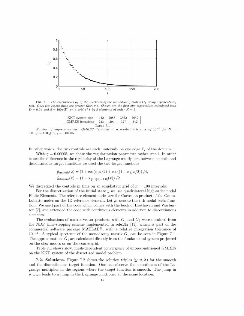
Fig. 7.1. The eigenvalues µi of the spectrum of the monodromy matrix G1 decay exponentiallyfast. Only few eigenvalues are greater than 0.5. Shown are the first 200 eigenvalues calculated withD = 0.01 and β = 100χ(Γ) on a grid of 8-by-8 elements of order K = 5.

KKT system size 442 2083 3562 7642GMRES iterations 223 294 327 342

Table 7.1Number of unpreconditioned GMRES iterations to a residual tolerance of 10−6 for D =

0.01, β = 100χ(Γ), γ = 0.00005.

In other words, the two controls act each uniformly on one edge Γi of the domain.With γ = 0.00005, we chose the regularization parameter rather small. In order

to see the difference in the regularity of the Lagrange multipliers between smooth anddiscontinuous target functions we used the two target functions

ysmooth(x) = (2 + cos(x1π/2) + cos((1− x2)π/2)) /4,

ydiscont(x) =(1 + χ[0,1]×[−1,0](x)

)/2.

We discretized the controls in time on an equidistant grid of m = 100 intervals.For the discretization of the initial state y we use quadrilateral high-order nodal

Finite Elements. The reference element nodes are the Cartesian product of the Gauss-Lobatto nodes on the 1D reference element. Let ϕi denote the i-th nodal basis func-tion. We used part of the code which comes with the book of Hesthaven and Warbur-ton [7], and extended the code with continuous elements in addition to discontinuouselements.

The evaluations of matrix-vector products with G1 and G2 were obtained fromthe NDF time-stepping scheme implemented in ode15s [13], which is part of thecommercial software package MATLABr, with a relative integration tolerance of10−11. A typical spectrum of the monodromy matrix G1 can be seen in Figure 7.1.The approximations G1 are calculated directly from the fundamental system projectedon the slow modes or on the coarse grid.

Table 7.1 shows slow, mesh-dependent convergence of unpreconditioned GMRESon the KKT system of the discretized model problem.

7.2. Solutions. Figure 7.2 shows the solution triples (y,u,λ) for the smoothand the discontinuous target function. One can observe the smoothness of the La-grange multiplier in the regions where the target function is smooth. The jump inydiscont leads to a jump in the Lagrange multiplier at the same location.

15

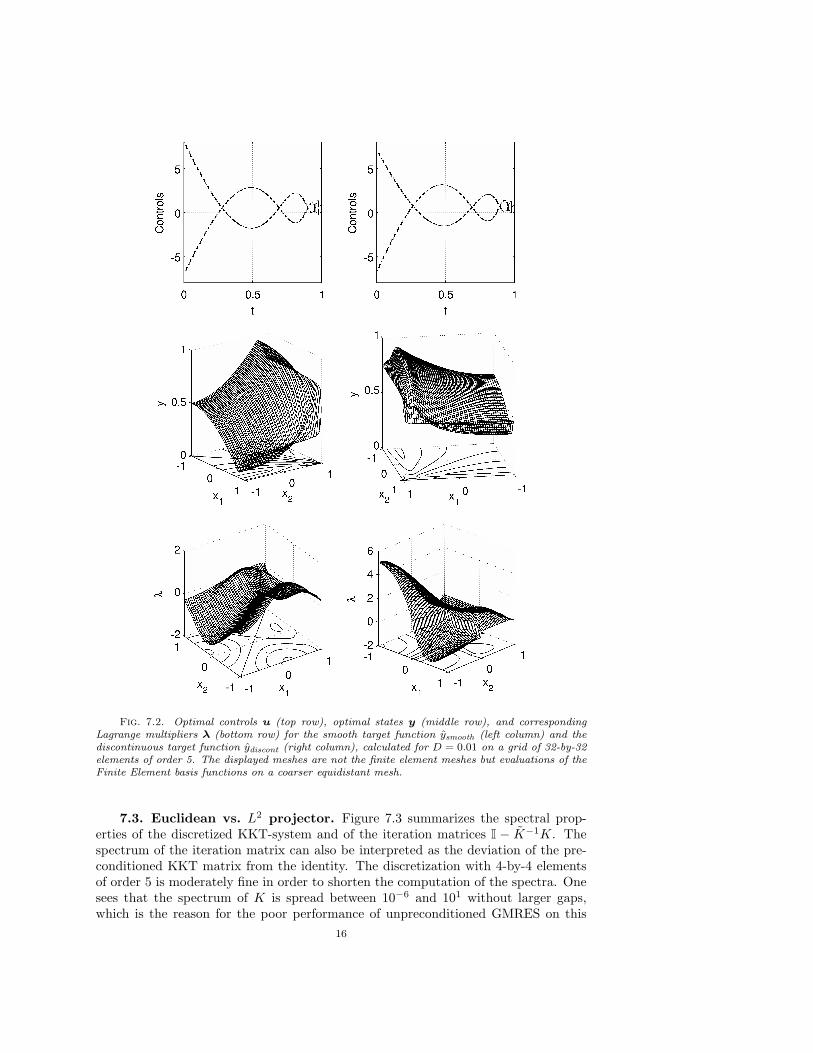
Fig. 7.2. Optimal controls u (top row), optimal states y (middle row), and correspondingLagrange multipliers λ (bottom row) for the smooth target function ysmooth (left column) and thediscontinuous target function ydiscont (right column), calculated for D = 0.01 on a grid of 32-by-32elements of order 5. The displayed meshes are not the finite element meshes but evaluations of theFinite Element basis functions on a coarser equidistant mesh.

7.3. Euclidean vs. L2 projector. Figure 7.3 summarizes the spectral prop-erties of the discretized KKT-system and of the iteration matrices I − K−1K. Thespectrum of the iteration matrix can also be interpreted as the deviation of the pre-conditioned KKT matrix from the identity. The discretization with 4-by-4 elementsof order 5 is moderately fine in order to shorten the computation of the spectra. Onesees that the spectrum of K is spread between 10−6 and 101 without larger gaps,which is the reason for the poor performance of unpreconditioned GMRES on this

16

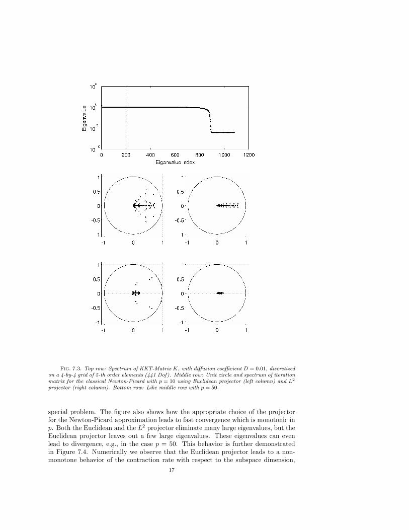
Fig. 7.3. Top row: Spectrum of KKT-Matrix K, with diffusion coefficient D = 0.01, discretizedon a 4-by-4 grid of 5-th order elements (441 Dof). Middle row: Unit circle and spectrum of iterationmatrix for the classical Newton-Picard with p = 10 using Euclidean projector (left column) and L2

projector (right column). Bottom row: Like middle row with p = 50.

special problem. The figure also shows how the appropriate choice of the projectorfor the Newton-Picard approximation leads to fast convergence which is monotonic inp. Both the Euclidean and the L2 projector eliminate many large eigenvalues, but theEuclidean projector leaves out a few large eigenvalues. These eigenvalues can evenlead to divergence, e.g., in the case p = 50. This behavior is further demonstratedin Figure 7.4. Numerically we observe that the Euclidean projector leads to a non-monotone behavior of the contraction rate with respect to the subspace dimension,

17

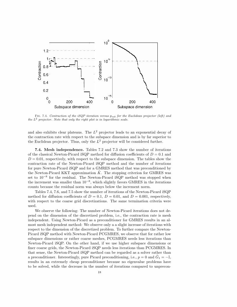
Fig. 7.4. Contraction of the iSQP iteration versus psub for the Euclidean projector (left) andthe L2 projector. Note that only the right plot is in logarithmic scale.

and also exhibits clear plateaus. The L2 projector leads to an exponential decay ofthe contraction rate with respect to the subspace dimension and is by far superior tothe Euclidean projector. Thus, only the L2 projector will be considered further.

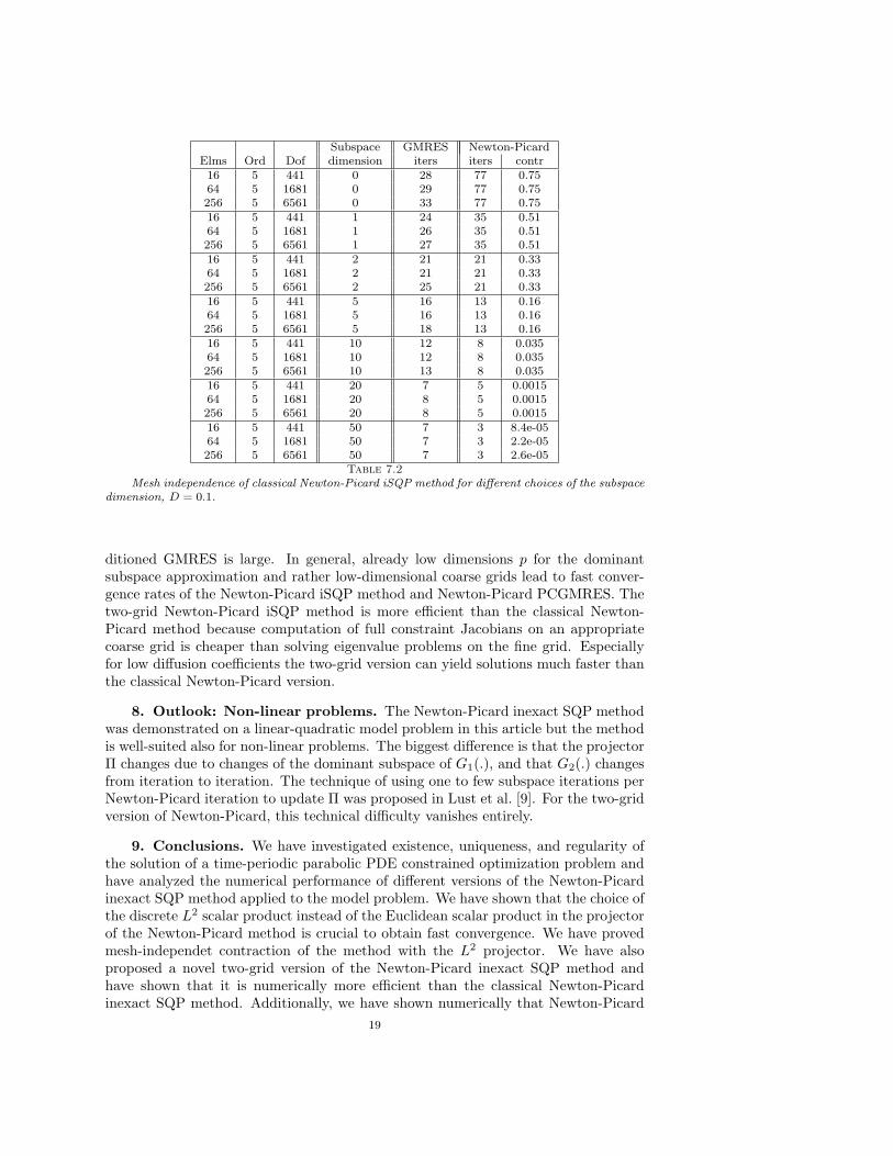
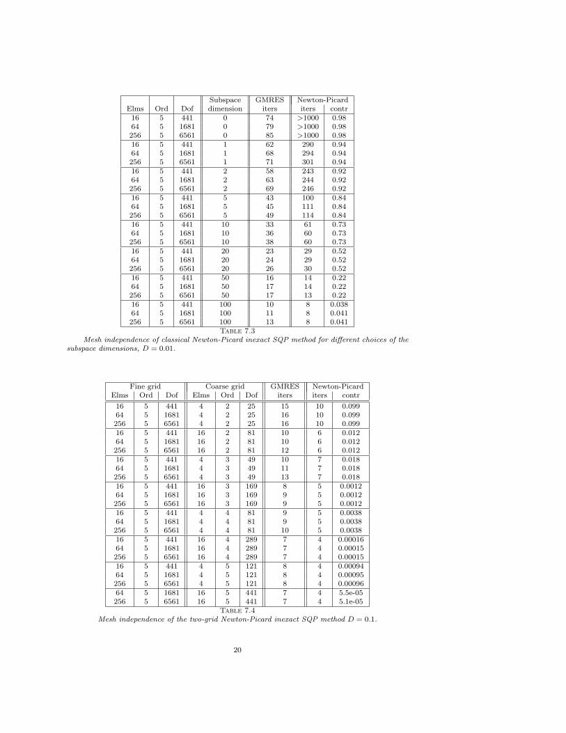
7.4. Mesh independence. Tables 7.2 and 7.3 show the number of iterationsof the classical Newton-Picard iSQP method for diffusion coefficients of D = 0.1 andD = 0.01, respectively, with respect to the subspace dimension. The tables show thecontraction rate of the Newton-Picard iSQP method and the number of iterationsfor pure Newton-Picard iSQP and for a GMRES method that was preconditioned bythe Newton-Picard KKT approximation K. The stopping criterion for GMRES wasset to 10−8 for the residual. The Newton-Picard iSQP method was stopped whenthe increment was smaller than 10−8, which slightly favors GMRES in the iterationscounts because the residual norm was always below the increment norm.

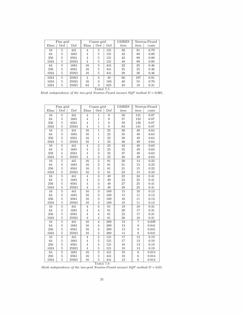
Tables 7.4, 7.6, and 7.5 show the number of iterations of the Newton-Picard iSQPmethod for diffusion coefficients of D = 0.1, D = 0.01, and D = 0.001, respectively,with respect to the coarse grid discretizations. The same termination criteria wereused.

We observe the following: The number of Newton-Picard iterations does not de-pend on the dimension of the discretized problem, i.e., the contraction rate is meshindependent. Using Newton-Picard as a preconditioner for GMRES results in an al-most mesh independent method: We observe only a a slight increase of iterations withrespect to the dimension of the discretized problem. To further compare the Newton-Picard iSQP method with Newton-Picard PCGMRES, we observe that for rather lowsubspace dimensions or rather coarse meshes, PCGMRES needs less iterations thanNewton-Picard iSQP. On the other hand, if we use higher subspace dimensions orfiner coarse grids, the Newton-Picard iSQP needs less iterations than PCGMRES. Inthat sense, the Newton-Picard iSQP method can be regarded as a solver rather thana preconditioner. Interestingly, pure Picard preconditioning, i.e., p = 0 and G1 = −I,results in an extremely cheap preconditioner because no eigenvalue problems haveto be solved, while the decrease in the number of iterations compared to unprecon-

18

Subspace GMRES Newton-PicardElms Ord Dof dimension iters iters contr

16 5 441 0 28 77 0.7564 5 1681 0 29 77 0.75256 5 6561 0 33 77 0.7516 5 441 1 24 35 0.5164 5 1681 1 26 35 0.51256 5 6561 1 27 35 0.5116 5 441 2 21 21 0.3364 5 1681 2 21 21 0.33256 5 6561 2 25 21 0.3316 5 441 5 16 13 0.1664 5 1681 5 16 13 0.16256 5 6561 5 18 13 0.1616 5 441 10 12 8 0.03564 5 1681 10 12 8 0.035256 5 6561 10 13 8 0.03516 5 441 20 7 5 0.001564 5 1681 20 8 5 0.0015256 5 6561 20 8 5 0.001516 5 441 50 7 3 8.4e-0564 5 1681 50 7 3 2.2e-05256 5 6561 50 7 3 2.6e-05

Table 7.2Mesh independence of classical Newton-Picard iSQP method for different choices of the subspace

dimension, D = 0.1.

ditioned GMRES is large. In general, already low dimensions p for the dominantsubspace approximation and rather low-dimensional coarse grids lead to fast conver-gence rates of the Newton-Picard iSQP method and Newton-Picard PCGMRES. Thetwo-grid Newton-Picard iSQP method is more efficient than the classical Newton-Picard method because computation of full constraint Jacobians on an appropriatecoarse grid is cheaper than solving eigenvalue problems on the fine grid. Especiallyfor low diffusion coefficients the two-grid version can yield solutions much faster thanthe classical Newton-Picard version.

8. Outlook: Non-linear problems. The Newton-Picard inexact SQP methodwas demonstrated on a linear-quadratic model problem in this article but the methodis well-suited also for non-linear problems. The biggest difference is that the projectorΠ changes due to changes of the dominant subspace of G1(.), and that G2(.) changesfrom iteration to iteration. The technique of using one to few subspace iterations perNewton-Picard iteration to update Π was proposed in Lust et al. [9]. For the two-gridversion of Newton-Picard, this technical difficulty vanishes entirely.

9. Conclusions. We have investigated existence, uniqueness, and regularity ofthe solution of a time-periodic parabolic PDE constrained optimization problem andhave analyzed the numerical performance of different versions of the Newton-Picardinexact SQP method applied to the model problem. We have shown that the choice ofthe discrete L2 scalar product instead of the Euclidean scalar product in the projectorof the Newton-Picard method is crucial to obtain fast convergence. We have provedmesh-independet contraction of the method with the L2 projector. We have alsoproposed a novel two-grid version of the Newton-Picard inexact SQP method andhave shown that it is numerically more efficient than the classical Newton-Picardinexact SQP method. Additionally, we have shown numerically that Newton-Picard

19

Subspace GMRES Newton-PicardElms Ord Dof dimension iters iters contr

16 5 441 0 74 >1000 0.9864 5 1681 0 79 >1000 0.98256 5 6561 0 85 >1000 0.9816 5 441 1 62 290 0.9464 5 1681 1 68 294 0.94256 5 6561 1 71 301 0.9416 5 441 2 58 243 0.9264 5 1681 2 63 244 0.92256 5 6561 2 69 246 0.9216 5 441 5 43 100 0.8464 5 1681 5 45 111 0.84256 5 6561 5 49 114 0.8416 5 441 10 33 61 0.7364 5 1681 10 36 60 0.73256 5 6561 10 38 60 0.7316 5 441 20 23 29 0.5264 5 1681 20 24 29 0.52256 5 6561 20 26 30 0.5216 5 441 50 16 14 0.2264 5 1681 50 17 14 0.22256 5 6561 50 17 13 0.2216 5 441 100 10 8 0.03864 5 1681 100 11 8 0.041256 5 6561 100 13 8 0.041

Table 7.3Mesh independence of classical Newton-Picard inexact SQP method for different choices of the

subspace dimensions, D = 0.01.

Fine grid Coarse grid GMRES Newton-PicardElms Ord Dof Elms Ord Dof iters iters contr

16 5 441 4 2 25 15 10 0.09964 5 1681 4 2 25 16 10 0.099256 5 6561 4 2 25 16 10 0.09916 5 441 16 2 81 10 6 0.01264 5 1681 16 2 81 10 6 0.012256 5 6561 16 2 81 12 6 0.01216 5 441 4 3 49 10 7 0.01864 5 1681 4 3 49 11 7 0.018256 5 6561 4 3 49 13 7 0.01816 5 441 16 3 169 8 5 0.001264 5 1681 16 3 169 9 5 0.0012256 5 6561 16 3 169 9 5 0.001216 5 441 4 4 81 9 5 0.003864 5 1681 4 4 81 9 5 0.0038256 5 6561 4 4 81 10 5 0.003816 5 441 16 4 289 7 4 0.0001664 5 1681 16 4 289 7 4 0.00015256 5 6561 16 4 289 7 4 0.0001516 5 441 4 5 121 8 4 0.0009464 5 1681 4 5 121 8 4 0.00095256 5 6561 4 5 121 8 4 0.0009664 5 1681 16 5 441 7 4 5.5e-05256 5 6561 16 5 441 7 4 5.1e-05

Table 7.4Mesh independence of the two-grid Newton-Picard inexact SQP method D = 0.1.

20

Fine grid Coarse grid GMRES Newton-PicardElms Ord Dof Elms Ord Dof iters iters contr

16 5 441 4 5 121 38 81 0.7964 5 1681 4 5 121 42 89 0.80256 5 6561 4 5 121 42 89 0.801024 5 25921 4 5 121 48 89 0.8064 5 1681 16 5 441 22 25 0.46256 5 6561 16 5 441 25 25 0.461024 5 25921 16 5 441 29 26 0.46

1024 5 25921 4 3 49 66 197 0.911024 5 25921 16 3 169 40 55 0.701024 5 25921 64 3 625 23 18 0.31

Table 7.5Mesh independence of the two-grid Newton-Picard inexact SQP method D = 0.001.

Fine grid Coarse grid GMRES Newton-PicardElms Ord Dof Elms Ord Dof iters iters contr

16 5 441 4 1 9 50 131 0.8764 5 1681 4 1 9 57 132 0.87256 5 6561 4 1 9 59 136 0.871024 5 25921 4 1 9 63 141 0.8716 5 441 16 1 25 30 49 0.6464 5 1681 16 1 25 35 49 0.64256 5 6561 16 1 25 38 49 0.641024 5 25921 16 1 25 40 49 0.6416 5 441 4 2 25 32 49 0.6364 5 1681 4 2 25 35 49 0.63256 5 6561 4 2 25 37 49 0.631024 5 25921 4 2 25 40 49 0.6316 5 441 16 2 81 20 14 0.2364 5 1681 16 2 81 21 15 0.23256 5 6561 16 2 81 21 15 0.231024 5 25921 16 2 81 23 15 0.2316 5 441 4 3 49 22 24 0.4164 5 1681 4 3 49 24 25 0.41256 5 6561 4 3 49 27 25 0.411024 5 25921 4 3 49 29 25 0.4116 5 441 16 3 169 15 10 0.1364 5 1681 16 3 169 15 11 0.13256 5 6561 16 3 169 16 11 0.131024 5 25921 16 3 169 18 11 0.1316 5 441 4 4 81 19 18 0.3164 5 1681 4 4 81 20 17 0.31256 5 6561 4 4 81 22 17 0.311024 5 25921 4 4 81 26 18 0.3116 5 441 16 4 289 12 7 0.03964 5 1681 16 4 289 13 8 0.041256 5 6561 16 4 289 13 8 0.0411024 5 25921 16 4 289 14 8 0.04116 5 441 4 5 121 17 13 0.1964 5 1681 4 5 121 17 13 0.19256 5 6561 4 5 121 18 13 0.191024 5 25921 4 5 121 19 13 0.1964 5 1681 16 5 441 10 6 0.014256 5 6561 16 5 441 10 6 0.0141024 5 25921 16 5 441 12 6 0.014

Table 7.6Mesh independence of the two-grid Newton-Picard inexact SQP method D = 0.01.

21

inexact SQP can serve an efficient preconditioner for the solution of the KKT systemwith GMRES.

References.[1] A. Agarwal, L.T. Biegler, and S.E. Zitney. Simulation and optimization of pres-

sure swing adsorption systems using reduced-order modeling. Ind. Eng. Chem.Res., 48(5):2327–2343, 2009.

[2] V. Barbu. Optimal control of linear periodic resonant systems in Hilbert spaces.SIAM J. Control Optim., 35(6):2137–2156, 1997.

[3] H.G. Bock, W. Egartner, W. Kappis, and V. Schulz. Practical shape optimizationfor turbine and compressor blades by the use of PRSQP methods. Optim. Eng.,3(4):395–414, 2002.

[4] A. Borzı. Multigrid methods for parabolic distributed optimal control problems.J. Comput. Appl. Math., 157(2):365 – 382, 2003.

[5] A. Griewank and A. Walther. On constrained optimization by adjoint basedQuasi-Newton methods. Optim. Method. Softw., 17:869–889, 2002.

[6] S.B. Hazra, V. Schulz, J. Brezillon, and N.R. Gauger. Aerodynamic shape opti-mization using simultaneous pseudo-timestepping. J. Comput. Phys., 204(1):46– 64, 2005.

[7] Jan S. Hesthaven and Tim Warburton. Nodal Discontinuous Galerkin Methods,volume 54 of Texts in Applied Mathematics. Springer New York, 2008.

[8] Y. Kawajiri and L.T. Biegler. Optimization strategies for Simulated Moving Bedand PowerFeed processes. AIChE J., 52(4):1343–1350, 2006.

[9] K. Lust, D. Roose, A. Spence, and A. R. Champneys. An adaptive Newton-Picardalgorithm with subspace iteration for computing periodic solutions. SIAM J. Sci.Comput., 19(4):1188–1209, July 1998.

[10] S. Nilchan and C. Pantelides. On the optimisation of periodic adsorption pro-cesses. Adsorption, 4:113–147, 1998.

[11] A. Potschka, Hans Georg Bock, S. Engell, A. Kupper, and Johannes P.Schloder. A Newton-Picard inexact SQP method for optimization of SMBprocesses. Preprint SPP1253-01-01, University of Heidelberg, 2008. URLhttp://www.am.uni-erlangen.de/home/spp1253.

[12] M. Renardy and R.C. Rogers. An Introduction to partial Differential Equations,volume 13 of Texts in Applied Mathematics. Springer-Verlag, New York, Berlin,Heidelberg, 1992.

[13] L.F. Shampine and M.W. Reichelt. The MATLAB ODE suite. SIAM J. Sci.Comput., 18(1):1–22, 1997.

[14] A. Toumi, S. Engell, M. Diehl, H.G. Bock, and J.P. Schloder. Efficient opti-mization of Simulated Moving Bed Processes. Chem. Eng. Process., 46 (11):1067–1084, 2007. (invited article).

[15] C. Trenchea. Periodic optimal control of the Boussinesq equation. NonlinearAnal., 53:81–96, 2003.

[16] F. Troltzsch. Optimale Steuerung partieller Differentialgleichungen: Theorie,Verfahren und Anwendungen. Vieweg+Teubner Verlag, Wiesbaden, 1st edition,2005.

[17] T.L. van Noorden, S.M. Verduyn Lunel, and A. Bliek. Optimization of cyclicallyoperated reactors and separators. Chem. Eng. Sci., 58:4114–4127, 2003.

[18] J. Wloka. Partielle Differentialgleichungen: Sobolevraume u. Randwertaufgaben.B.G. Teubner, Stuttgart, 1982.

22