NASA/CR- 1998-208436

ICASE Report No. 98-25

A New Time-space Accurate Scheme for Hyperbolic

Problems h Quasi-explicit Case

David Sidilkover

ICASE, Hampton, Virginia

Institute for Computer Applications in Science and Engineering

NASA Langley Research Center

Hampton, VA

Operated by Universities Space Research Association

National Aeronautics and

Space Administration

Langley Research Center

Hampton, Virginia 23681-2199

Prepared for Langley Research Center underContracts NAS 1-19480 and NAS 1-97046

October 1998

https://ntrs.nasa.gov/search.jsp?R=19990008127 2018-05-30T18:31:02+00:00Z

Available from the following:

NASA Center for AeroSpace Information (CASI)

7121 Standard Drive

Hanover, MD 21076-1320

(301) 621-0390

National Technical Information Service (NTIS)

5285 Port Royal Road

Springfield, VA 22161-2171

(703) 487-4650

11 Ii

A NEW TIME-SPACE ACCURATE SCHEME FOR HYPERBOLIC PROBLEMS I"

QUASI-EXPLICIT CASE*

DAVID SIDILKOVERt

Abstract. This paper presents a new discretization scheme for hyperbolic systems of conservation

laws. It satisfies the TVD property and relies on the new high-resolution mechanism which is compatible

with the genuinely multidimensional approach proposed recently. This work can be regarded as a first step

towards extending the genuinely multidimensional approach to unsteady problems. Discontinuity capturing

capabilities and accuracy of the scheme are verified by a set of numerical tests.

Key words, unsteady problems, high-resolution schemes, TVD property.

Subject classification. Applied and Numerical Mathematics.

1. Introduction. A general approach towards the construction of genuinely multidimensional high-

resolution schemes for hyperbolic systems was proposed recently ([16],[15],[17]). The main advantage of this

approach is that it results in the discrete schemes that have some desirable properties which allow to design

very efficient steady solvers (see [13] for a summary). However, these discretizations are suitable exclusively

for steady problems since they are second order accurate at the steady-state only.

Extending of the genuinely multidimensional approach to the transient problems may seem at the first

sight straightforward. Noting that the unsteady advection problem in one dimensions is very similar to the

steady advection problem in two dimensions, one can apply, say, the "fluctuation-splitting" (or "residual

distribution") steady 2D advection scheme for triangular meshes (proposed in [3] and given an algebraic

formulation using limiters in [19]) to a one dimensional unsteady problem as well. However, a closer look

reveals that the result of such a straightforward application may be that the "present" depends on the

"future". One could leave the causality concerns to the philosophers and try to iterate back and forth in

space-time. However, the memory requirements of this approach will become absurdly demanding in more

than one spatial dimension, since all the time instances need to bc stored.

This paper presents a new discrete scheme for the hyperbolic conservation laws and systems of conser-

vation laws. It is one-step one-stage and satisfies the TVD property. The key feature of the new scheme is

that it relies on the non-standard high-resolution mechanism which is compatible with the genuinely mul-

tidimensional approach proposed recently and will allow to extend it to unsteady problems. The scheme is

formulated using the framework introduced by Sweby [21], which makes it plain what are the differences

and similarities between the proposed and the existing discretizations. The new scheme has links to the 2D

steady advection control volume scheme constructed in [14],[18]. As the first stage we address only the case

of Courant number less than one. The constructed scheme is not explicit even in this case. However, the

treatment of the discrete equations can be made sufficiently similar to explicit (see §3). That is why we call

the approach "quasi-explicit". We verify the accuracy and the discontinuity capturing properties of the new

scheme and demonstrate that the quality of the solutions obtained using it is at least as good as when using

the standard schemes.

*This work was supported by the National Aeronautics and Space Administration under NASA Contract Nos. NASl-19480

and NAS1-97046 while the author was in residence at the Institute for Computer Applications in Science and Engineering

(ICASE), NASA Langley Research Center, Hampton, VA 23681-2199.

tICASE, Mail Stop 403, NASA Langley Research Center, Hampton, VA 23681

The goal of this research direction is to construct vcry efficient implicit solvcrs for thc unsteady com-

pressible flow equations. The unsteady genuinely-multidimensional schemes are expected to allow this since

they should maintain some fundamental properties of their steady ancestors: a good measure h-ellipticity of

the implicit discretizations and the possibility to distinguish between different co-factors of the systems of

equations. Therefore, the next step will be to consider the implicit case (Courant number larger than one)

and to design an efficient implicit solver. This study will be reported elsewhere.

The paper is organized as follows: §2 contains the description of the scheme (in control volume formu-

lation) and the discussion concerning some basic properties. A possible solution procedure for the discrete

equations is presented in §3. Generalization of the scheme to the Euler system is given in §4. §5 reports

the numerical tests conducted with the constructed scheme. Some conclusions and discussion regarding the

future research directions are presented in §6. The residual-distribution (fluctuation-splitting) formulation

of the scheme is given in Appendix A. Also a brief discussion on more general conditions for a scheme to be

TVD is given in Appendix B.

2. The new scheme and its basic properties. Consider first an initial value problem for a scalar

conservation law

(2.1) ut + f(u)_ = 0, t _> 0, z E ]I{,u(z, 0) = u0(x).

Following Sweby [21] we shall use the following simplified notation (unless specified othcrwisc) for the data

on the new and old time levels respectively

Un+l(2.2) uk=-- k , Uk-- U'_.

A gencral conservative discretization of (2.1) can be given as follows

(2.3) u k ----uk - )_(hk+ ½ -- hk_½ )

wherc hk+ ½ is the consistent numerical flux

hk+½= uk+m.1, uk-m, ... ,uh(u,.-.,

(2.4)

and )_ is the mesh ratio

At

(2.5) _ = _.

A crucial property needed for convergence proof of the difference scheme (2.3) is the so-called Total Variation

Diminishing (TVD) property [4]

(2.6) TV(u "+1) < TV(un),

where, abolishing temporarily the notation (2.2), we define the Total Variation an time level n as

(2.7) TV(un) = E lu'k+ 1 - u'_lTt

If the scheme (2.3) can be written in the form

(2.8) u k = Uk -- Ck_½ AUk_ ½ -t- Dk+½ AUk+ ½,

!l | i

thenasufficientconditionfortheschemeto beTVD (Harten'sLemma,see[4])is thatthc (data-dependent)coefficientssatisfytheinequalities

(2.9)

and

(2.10)

0< Ck+½, 0 < Dk+½,

O < Ck+ ½ + Dk+ ½ <_1.

2.1. First order upwind scheme. Consider first for the purpose of illustration the first order upwind

scheme.

Define the local propagation speed

(2.11)

where

(2.12) Ark+½ = f(Uk+l) -- f(uk), Auk+_ = Uk+l -- Uk.

A numerical flux defining a first order upwind scheme can be written as follows

1h_+½ = -_[(Y(uk) + f(uk+l)) - lak+½IAuk+_].(2.13)

Denote

(2.14)

and

= _(ak+½ + lak+_l)a k++ ½ 1

= l(ak, ½ak+½ - lak+½ I)

(2.15) Vk+ ½ = )_aL ½

"k-+i = _%-+½'

The local OFL number then can be written as follows

(2.16) _k+½ = Aak+½ = v++½ + _k+½"

It is easy to see that using (2.14),(2.15) the scheme defined by (2.13) will read as

(2.17) u k = Uk -- vk+ ½Au k_ ½ -- "k-+ ½AUk+ ½

Denoting

(2.18) Ck+ ½ = _,++½, Ok+ ½ = -5-+3

makes it obvious that inequality (2.9) is satisfied, and that

(2.19) Ck+ ½ + Dk+ ½ + -= "k+i - %+½ = l_k+il -<1

is a CFL condition. Therefore, the first order upwind scheme is TVD.

tk-1

k0- n+l

f_.-1/2 ft+t/2

@ @ nk k+l

FIG. 1. Stencil of the Lax- Wendroff scheme.

2.2. The high-resolution scheme: constant coefficient equation. In order to illustrate the con-

struction of a high-resolution scheme we shall consider first a linear constant coefficient equation

(2.20) ut + au_ = O, a > O.

The first order upwind scheme approximating (2.20) can bc written as follows

u k =uk--t/Au k _(2.21)

where

(2.22)aAt

Ax

is the CFL number. The second order Lax-Wendroff [6] scheme can be given as follows (the corresponding

stencil is depicted on Fig.l)

(2.23) uk = uk - vAuk_½ - A_[_(1 - v)_Auk÷_]

or as a first order upwind scheme (2.21) whose flux (2.13) is augmented by the following anti-diffusive flux

1(2.24) 2)_ (1 - v)VAUk+ ½

2.2.1. Some existing schemes. The Lax-Wendroff (as well as any second order linear scheme) is

known not to satisfy the TVD property. A high-resolution scheme can be defined by adding a "limited"

anti-diffusive flux to the first order upwind one. The resulting scheme reads as follows

(2.25) u k = uk -- VAUk_½ -- A-[¢(qk)_(1 -- v)uAuk+_],

where qk is standardly defined as a ratio of two subsequent finite differences of the numericM solution on the

time-level n

(2.26)

Noting that the following identity holds

Au k_ ½

qk = AUk+ _ •

¢ (qk) Au k- ½'(2.27) ¢(qk)Auk+½ --= qk

it can be concluded (see [21]) that high-resolution scheme (2.25) can be viewed as a nonlincar hybrid of Lax-

Wendroff and the Warming-Beam [22] schemes. The latter is given by the following (the stencil is depicted

!i _

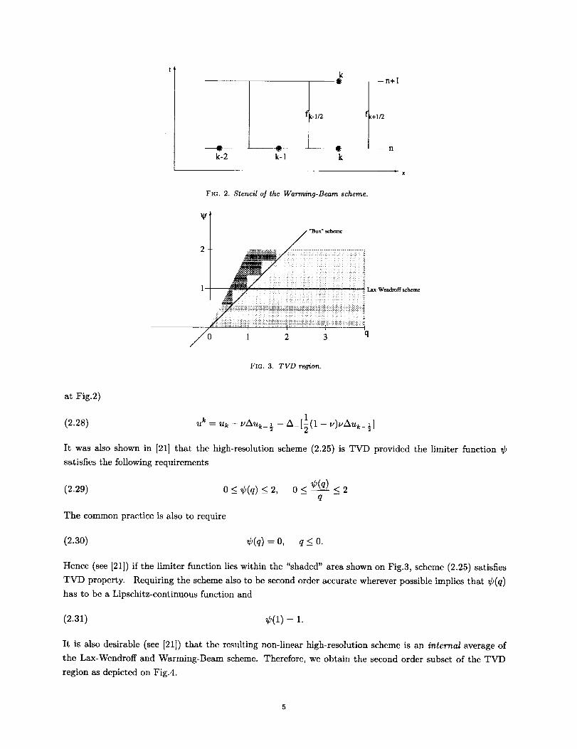
k-2 k-1

k

t,2ik

FIG. 2. Stencil of the Warming-Beam scheme.

¥

-n+l

rl

Lax-Wendmff scheme

1 2 3

FIG. 3. TVD region.

at Fig.2)

|(2.28) _t k

= uk - VAUk_ ½ -- A-[2(1 -- v)vAuk_½]

It was also shown in [21] that the high-resolution scheme (2.25) is TVD provided the limiter function ¢

satisfies the following requirements

(2.29) 0 < ¢(q) _< 2,

The common practice is also to require

(2.30) ¢(q) = 0, q _< 0.

Hence (see [21]) if the limiter function lies within the "shaded" area shown on Fig.3, scheme (2.25) satisfies

TVD property. Requiring the scheme also to be second order accurate wherever possible implies that ¢(q)

has to be a Lipschitz-continuous function and

(2.31) ¢(1) = 1.

It is also desirable (see [21]) that the resulting non-linear high-resolution scheme is an internal average of

the Lax-Wendroff and Warming-Beam schemc. Therefore, we obtain the second order subsct of the TVD

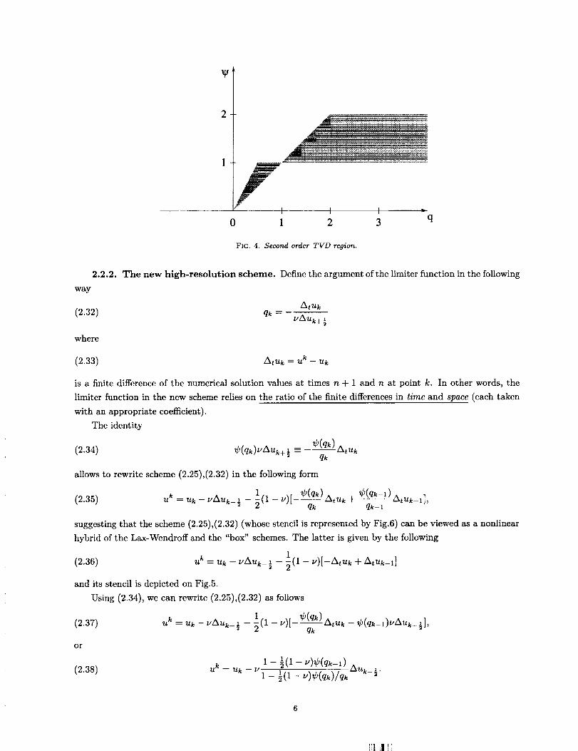
region as depicted on Fig.4.

2

fI I I _"

0 1 2 3 q

FIG. 4, Second order TVD region.

2.2.2.

way

Atuk

(2.32) qk = VAUk+½

where

(2.33) Atuk = u k -- Uk

The new hlgh-resolution scheme. Define the argument of the limiter function in the following

is a finite difference of the numerical solution values at times n + 1 and n at point k. In other words, the

limitcr function in the new scheme relies on the ratio of the finite differences in time and space (each taken

with an appropriate coefficient).

The identity

(2.34) ¢(qk)VAUk+ ½ :_- ¢(qk) Atukqk

allows to rewrite scheme (2.25),(2.32) in the following form

(2.35) u k = Uk -- VAUk_ ½ -- 1(1 -- v)[--¢(qk) Atuk + ¢(qk-1--------_)Atuk-l],qk qk- 1

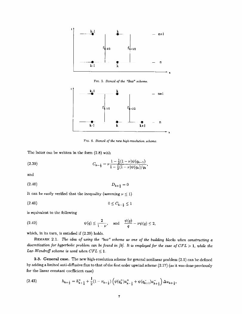
suggesting that the scheme (2.25),(2.32) (whose stencil is represented by Fig.6) can be viewed as a nonlinear

hybrid of the Lax-Wendroff and the "box" schemes. The latter is given by the following

(2.36) u k = uk -- _'Auk_½ -- 1(1 - v)[--AtUk + AtILk-1]

and its stencil is depicted on Fig.5.

Using (2.34), we can rewrite (2.25),(2.32) as follows

= u_ - .A_k_½ - ½(1- _,)[_¢(qk) A_k -- ¢(qk__)_A_k_½1,U k

qk(2.37)

or

(2.38) - ½(1- u)¢(qk-1) AUk_].uk ---uk -- v__ ½(1-- v)¢(qk)/qk

i! ! !

k-1

k

f -1/2 1/2

k

Fxc. 5. Stencil of the "Box" scheme,

k-1 k--@ •

k-1 k k+l

FIG. 6. Stencil of the new high-resolution scheme.

n+l

n+l

The latter can be written in the form (2.8) with

(2.39)

and

(2.40) Dk+ ½ = 0

It can be easily verified that the inequality (assuming v < 1)

o < ck_½ < 1(2.41)

is equivalent to the following

1 -- 1(1 -- U)¢(qk_l)

Ck_ ½ ----V 1 __ 1(1 - v)¢(qk)/q k '

(2.42) _b(q) < 2 and ¢(q---_)- re(q) < 2,- 1-v' q -

which, in its turn, is satisfied if (2.29) holds.

REMARK 2.1. The idea of using the "box" scheme as one of the building blocks when constructing a

discretization for hyperbolic problem can be found in [9]. It is employed for the case of CFL > 1, while the

Lax-Wendroff scheme is used when CFL < 1.

2.3. General case. The new high-resolution scheme for general nonlinear problem (2.1) can be defined

by adding a limited anti-diffusive flux to that of the first order upwind scheme (2.17) (as it was done previously

for the linear constant coefficient case)

1 + + _3(qk+l)a--½_k+)(2.43) hk+ ] = hk+ ½+ _(1 - Vk+½) (¢(qk)ak+½ + Auk+½,

where

(2.44) q+k --_

and

(2.45) qk+l =

/akt U k

Aa++½Auk+½

ht_k+l

_%+ ½Auk+½

Using the identities

(2.46) + + Auk+ L --¢(qk )ak+]

and

(2.47) ¢(q-_+l)a;+½ AUk+½ --

the alternative form of the numerical flux (2.43) can be obtained

(2.4s)

Define

(2.49)

and

(2.50)

Denoting

(2.51)

¢(q+) Atuk

q+ )_

¢(qk+l) AtUk+l

qk-+l A '

(¢(q+)Atuk ¢(qk-+l) At )hk+½=h_+]- (1-vk+½) _, q+ _ + qk--+l _k+l .

+ 1 + +#k+½ = _¢(qk)v/_+½ (1 -- uk+½) ,

_+ 1¢(qk)(1 += - _k+½)#k+ ½ 2 qk

1 _ __ 1 ¢(qk+l)(1 -- uk-+½).#_-+½ = _¢(qk+l)u_-+½(1 --Yk+½), #k+] -- 2 qk+l

u+ ½(1 - pk+ ½)

G-½ = l_p+ , __k-_ - #k+½

and

(2.52) Dk+½ = 1 -+ -- '- gk- ½ - Pk+ ½

the scheme (2.3) with numerical fluxes defined by (2.43) (or (2.48)) can be put into form (2.8).

Finally, we can state the following result

THEOREM 2.2. Scheme (2.3) with high resolution flux (2.43) that incorporates a limiter function satis-

fying (2.29) is TVD.+ -+ -+

Proof. Note that if uk_ ½ > 0, then #k-½ = 0. Also, if vk++½ > 0, then Pk+½ = 0. It follows from herethat

(2.53) Ca_ ½ > O, Dk+ ½ > O,

provided the limiter function ¢ satisfies inequality (2.29).

13 !1

Inequality(2.29)givesthefollowing

(2.54) Ok+ ½ < 1, Dk+ ½ < 1,

However, since either +t_k+ ] or r'k+ ½ vanishes, either Ck+ ½ or Dk+ ½ will vanish as well. Therefore,

(2.55) Ck+ ½ + Dk+ ] < 1,

which together with (2.53) completes the proof. [:]

REMARK 2.3. Notice that a purely upwind decomposition (2._)-(2._5) is necessary here for the con-

struction, as the ratio between the numerator and denominator must be close to 1 in smooth monotone regions

in order to keep accuracy. In particular, a Lax-Friedrichs type splitting cannot be used here.

3. Solution procedure. Consider for simplicity scheme (2.25) with (2.32), devised for linear problem

(2.20). This scheme is not explicit the stencil involves more than one point on the new time level n + 1

(Fig.6). However, there is no need for a global solver in this case. One can use some simple local procedures

for solving procedures for solving the resulting discrete equations.

Space marching.

An obvious possibility is a space marching, i.e. solve the discrete equation at point k after it has been

solved at point k - 1. However, considering solving the nonlinear systems of equations and/or extensions to

multi-dimensions, it appears that the latter method may be not always feasible/desirable.

Predictor- Corrector.

Consider an initial-boundary value problem for (2.20) discretized on a grid k = 0, ...K. Assume, that

uk, the solution on the time level n, is a monotonic function.

Considcr an arbitrary discrete function u kt as an initial guess for a solution at the time lcvcl n + 1.

Performing one sweep of Jacobi relaxation using scheme (2.25) with (2.32) will result in u k*, i = 0, ..., K.

We can state the following

LEMMA 3.1. If the discrete function uk, k = O,...,K is monotonic, then the discrete function uk* is

monotonic as well.

Proof. Putting scheme (2.25),(2.32) into form (2.8) with Ck_], Ok+ ] defined by (2.39),(2.41) and (2.39)respectively, we can conclude that

(3.1) min(uk_l, Uk) < u k* < max(uk-1, Uk),

which concludes the proof. D

This suggests that the following predictor-corrector procedure can be used for solving the discrete equa-

tions resulting from the limited scheme:

Predictor. Lax-Wendroff scheme to produce a grid-function ukt, k = 0, ..., K, which is a second order

accurate solution to (2.1), but may exhibit an oscillatory behavior near discontinuities;

Corrector. Perform a Jacobi relaxation to update values u kt to obtain a new grid-function u k, k = O, ..., K

that is non-oscillatory (due to Lemma 3.1) and second order accurate solution to (2.1).

Such a solution procedure is essentially a point-implicit solver. Note that the resulting discrete function may

not in general satisfy the discrete equations corresponding either to the limited scheme or to thc Lax-Wendroff

scheme.

This should not cause any problems in the smooth regions since the discrepancy between the solutions

to two different second order schemes is expected to second order small.

Thedifficultythoughmayarisein thevicinityofdiscontinuities.Differentschemesmayresultindifferentdiscontinuityprofiles.Therefore,if theresidualsofoneschemearemeasuredonthesolutioncorrespondingto anotherscheme,theymaybe large.If nospecialcareis taken,thismayhavea cumulativeeffectoverseveraltime-stepsandleadto wrongshockspeeds.

Ourexperiencethoughdemonstrates,that it is sufficientto performafew(insteadof one)updatesofthesolutionin thevicinityof adiscontinuityusingthe "limited"schemeto makesurethat theresidualsofthisschemeareverysmall.Weshallelaborateonthisissuein thefuturepublicationwhichwill addressalsotheimplicitcase.

4. Hyperbolic systems.Weshallbrieflysketchoutanextensionofthenewschemetothehyperbolicsystemsofconservationlaws,in particular,to theEulerequationsofgasdynamics

(4.1) ut + f(u)_ :- 0

Again, as in the scalar case, the discretization can be put into the following general form

(4.2) u k = uk - A(hk+ ½ - hk_½)

. n+l(4.3) u k_u k , Uk--U_

For the case of the Euler equations we can take the Roe-averaged Jacobian matrix of f (see [11])

(4.4) Ak+½ (Uk+l -- Uk) = f(Uk+l) -- f(uk)

and define the first order upwind flux as follows

(4.5) h_+½ = [(f(uk) + f(uk+l)) - IAk+½I(uk+l - Uk)]

Here

(4.6)

T is the matrix of right eigenvectors of A, and

(4.7)

is a diagonal matrix

(4.8)

and its absolute value is defined as

(4.9)

IAk+½1= T[A[T -1,

A = T-1Ak+½T,

A : diag{al, ..., an}

IA[= diag{lall, ..., Ianl}.

We define the flux corresponding to the new high-resolution scheme as

u 1,w-li,.AD

hk+ ½ =hk+ ½+-_ ,1k_12 -r]

h AD -- (hi, ..., h,_) T

(4.10)

where the anti-diffusive flux is given by

(4.11)

10

and

(4.12)

with

(4.13)

= (1 +

a_At= /xz'

(4.14) q_ + At(wi)k=

(4.15) (qi)k-+ 1 = At (wi)k+l

)_(ai)k+½ A(wi)k+- _

and +(v_)k+½ and (vi)_+½ are the "positive" and "negative" parts of (_i)k+] respectively.

REMARK 4.1. Note that the formulated scheme (as well as any other scheme based on the pure upwind

decomposition) may produce non-physical solutions violating the entropy condition. Some ways to fix this

problem have been described in the literature (see, for instance, [5]). Therefore, we do not include a discussion

on this matter here.

5. Numerical results. In this section we present some numerical tests of the new scheme using a few

standard test problems.

5.1. Scalar case.

5.1.1. Linear advectlon equation. The purpose of this test is to verify the second order accuracy of

the method. Therefore, we use here a simple problem with the known exact solution.

Consider the initial-boundary value problem for the following equation

(5.1) ut + .5u_ = O.

on the domain [-1, 1] with the initial condition given by

(5.2) u(x, O) = -.5 sin 7rx + .5

and the boundary condition (at point x = -1)

(5.3) u(-1, t) ----.5 sin(1 + .5t) + .5.

It is obvious that the exact solution to this problem is given by

(5.4) u = -.5 sinrr(x - .5t) + .5.

The L1 error norm of the solution error at time t = 1.0 for different levels of resolution is presented in Table

5.1. The Courant number in all the tests is .5. The error reduction due to the doubling of the number of

the grid-points is roughly by factor 4, which verifies that the scheme is second order accurate for smooth

solutions.

11

TABLE 5.1

Linear advection equation: solution error LI norm behavior with the mesh refinement.

Number of grid-points

25

5O

100

2OO

Solution error (L1 norm)

0.0075311723

0.0018290140

0.0004250877

0.0000971690

Numerical order of accuracy

2.042

2.106

2.129

TABLE 5.2

Buyers equation: solution error L1 norm behamorwith the mesh refinement.

Number of grid-points Solution error (L1 norm) Numerical order of accuracy

50 0.0020134142

100 0.0005068036 1.990

0.0001261164200 2.007

5.1.2. Burgers equation. Our next purposc is to examine the accuracy of the new scheme as well as

its capability to resolve shocks, representing them by a sharp oscillation-free profile. The problem considered

here is the following nonlinear conservation law

(5.5) u, + .5(u_)_ = 0.

The following expression (raised sine) serves as the initial condition

(5.6) u(x, 0) = - sin(Trx) + 0.5

First we demonstrate the accuracy of the scheme for time t = .25 by comparing the solution error norm for

different levels of resolution (see Table5.2). In this case the solution is still smooth, since the shock did not

start to develop yet. The ability of the scheme to resolve shocks is demonstrated on the same test problem.

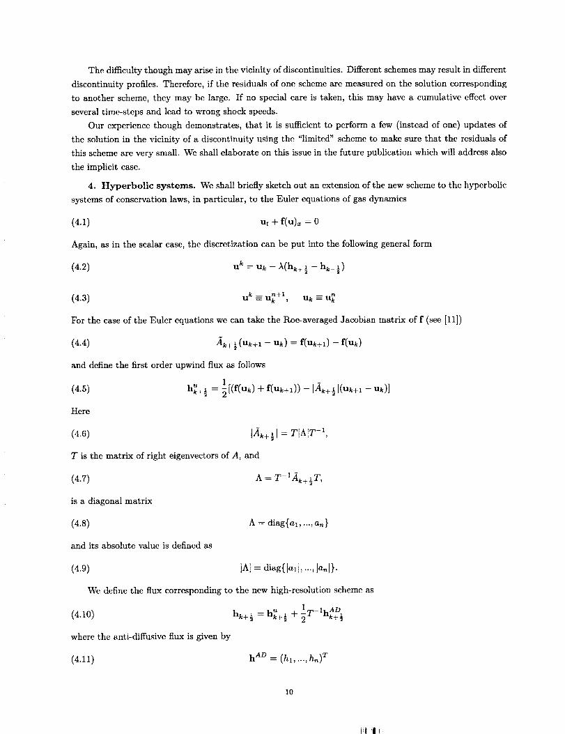
The numerical solution to this problem corresponding to time t = 2 is presented on Fig.7. Wc can see that

the shock is reprcscnted by a sharp layer and that there are no over- and undershoots on its sides.

5.2. Euler equations. In this section we present some numerical tests of the new scheme using a few

standard test problems concerning the Euler equations of gas dynamics. The scheme used is as described in

§4 with the Van Albada limiter. Note, that the Van Albada limitcr does not satisfy the inequalities (2.29)

(see Fig.12), which are a sufficient condition for a (scalar) scheme to be TVD. A more general sufficient

condition, that is satisfied by the Van Albada limiter, is presented in Appendix B. The reasons for using the

Van Albada limiter is discussed in Appendix B as well.

An the test-cases considered here use the domain 7P = {x : x E [-1, 1]}.

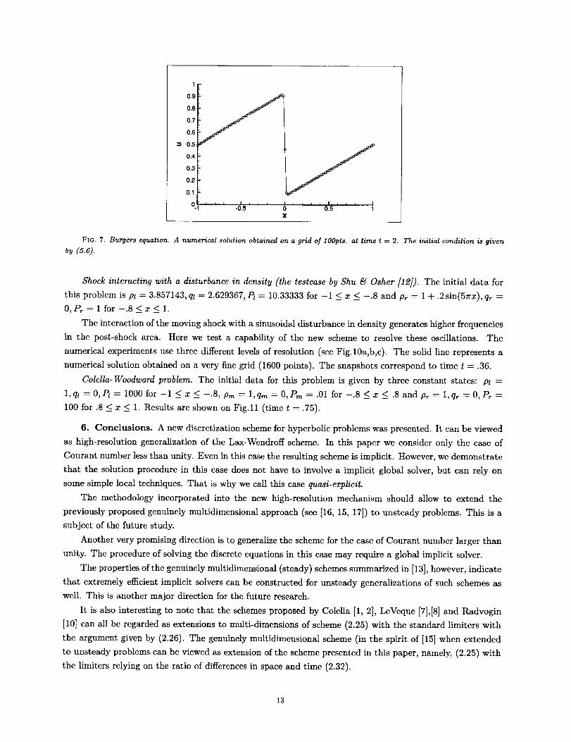
Lax's problem. The initial data for this problem are two constant states, one to the left of the origin

(-1 < x < 0): pt -- .445, qz = .698, Pt = 3.528, another to the right of the origin (0 < x < 1): p_ = .5, qr =

0, P_ = .571. Here p stands for density, q for velocity and P for pressure.

The numerical results for this case are presented on Fig.8. The computational grid is 200 points. Solid

lines represent the exact solution to the problem.

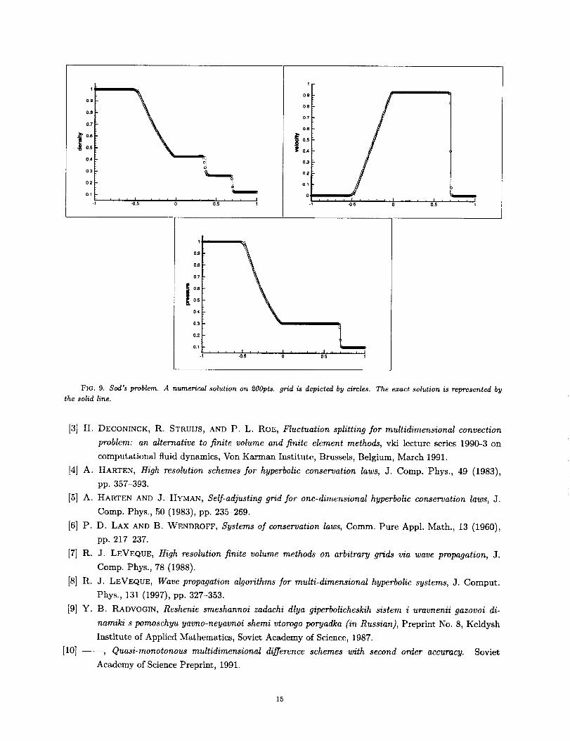
Sod's problem. Similarly to the previous problem, the initial data are given for the two constant states:

p_ = l,qt = 0,/_ = 1 and pr = .125, qr = 0, Pr = .1.

The grid consists of 200 points and the solid line represents the exact solution.

12

1

0.9

0.8

0.7

0.6

0.5

0.4

0.3

0.2

0.1

0 =llJl-0.5

Ji i I i I = i i = I

0 0.5 IX

FIG. 7. Burgers equation. A numerical solution obtained on a grid of lOOpts, at time t = 2. The initial condition is given

bu (5.6).

Shock interacting with a disturbance in density (the testcase by Shu _ Osher [12]). The initial data for

this problem is Pt = 3.857143, qt = 2.629367, Pl = 10.33333 for -1 < x < -.8 and Pr = 1 + .2 sin(57rx), qr =

0, Pr=l for -.8<x<l.

The interaction of the moving shock with a sinusoidal disturbance in density generates higher frequencies

in the post-shock area. Here we test a capability of the new scheme to resolve these oscillations. The

numerical experiments use three different levels of resolution (see Fig.10a,b,c). The solid line represents a

numerical solution obtained on a very fine grid (1600 points). The snapshots correspond to time t -- .36.

ColeUa-Woodward problem. The initial data for this problem is given by three constant states: Pt =

1, ql = 0, Pt = 1000 for -1 < x < -.8, Pm = 1,qm = 0, Pro = .01 for -.8 < x < .8 and p_ = 1,q_ = 0, P. =

100 for .8 < x < 1. Results are shown on Fig.ll (time t = .75).

6. Conclusions. A new discretization scheme for hyperbolic problems was presented. It can be viewed

as high-resolution generalization of the Lax-Wendroff scheme. In this paper we consider only thc case of

Courant number less than unity. Even in this case the resulting scheme is implicit. However, we demonstrate

that the solution procedure in this case does not havc to involve a implicit global solver, but can rely on

some simple local techniques. That is why we call this casc quasi-explicit.

The methodology incorporated into the new high-resolution mechanism should allow to extend thc

previously proposed genuinely multidimensional approach (see [16, 15, 17]) to unsteady problems. This is a

subject of the future study.

Another very promising direction is to generalize the scheme for the case of Courant number larger than

unity. The procedure of solving the discrete equations in this case may require a global implicit solver.

The properties of the genuinely multidimensional (steady) schemes summarized in [13], however, indicate

that extremely efficient implicit solvers can be constructed for unsteady generalizations of such schemes as

well. This is another major direction for the future research.

It is also interesting to note that the schemes proposed by Colella [1, 2], LeVeque [7],[8] and Radvogin

[10] can all be regarded as extensions to multi-dimensions of scheme (2.25) with the standard limiters with

the argument given by (2.26). The genuinely multidimensional scheme (in the spirit of [15] when extended

to unsteady problems can be viewed as extension of the scheme presented in this paper, namely, (2.25) with

the limiters relying on the ratio of differences in space and time (2.32).

13

1.3

1.2

1.1

t

0.911.8

0.7

11.6

11.5

0.4

11,3 i [ I v I i-0.5

h i t 10

, i I IllllllO.S 1

1.5

1.25

1

0,75

0.5

025

O:

__/, , p i I r

-O.Si i i 1 i

oi ,

05 1

35

3

2.5

i 2

1.5

I

0.5

-1i i i i I h i i k I .... I ,

-O.S 0 0.5

FIG. 8. Lax's problem. A numerical solution obtained on a grid of 20Opts. is represented by circles. The solid linecorresponds to the exact solution.

Consider a transient problem that converges to a steady-state. It is interesting to note that if the Lax-

Wendroff scheme (or one of its standard generalizations) is applied to solvc such a problem, the computed

steady-state solution will depend on the timc-stcp (since the artificial dissipation of such schemes scales with

the time-step). The scheme proposed in this paper, however (even though it is an extension of the Lax-

Wendroff scheme), will produce a steady-state solution that is independent of the time-step. This is due to

the fact that if the temporal changes of the solution become very small and eventually vanish, the limiter will

cut off all the spatial terms in the discretization that scale with the time-step. Thus, the scheme essentially

reduces to the first order upwind. The generalization of the scheme presented here to multi-dimensions is

expected to maintain this property to a certain extent as well.

Acknowledgments. The author would like to thank Chi-Wang Shu and Randall LcVeque for reading

the manuscript and making numerous very helpful comments.

REFERENCES

[1] P. COLELLA, Multidimensional upwind methods for hyperbolic conservation laws, Tech. Rep. LBL-17023,

Lawrence Berkeley Report, 1984.

[2] --, Multidimensional upwind methods for hyperbolic conservation laws, J. Comp. Phys., 87 (1990),

p. 171.

14

!_!I i

1

0.9

0.8

0.7

0.60.5

0.4

03

0.2

0.1

-1Illllill _,,lll_,l

_,5 0 0.5 1

0.01

o.e I

0.7 I

o.6 I

o_slo.4 I

0.3 I

o.2 I

o.1 I

e"

-IlllITll|

_.5 0J I r I i

O.E; 1

I

0.9

o.6

0.7

i 0.60.5

0,4

0.3

O2

0.1

-1I i I i I i I I l i i , | i , i I ]

-0.5 0 0.5 1

FIC. 9. Sod's problem. A numerical solution on $OOpts. grid is depicted by circles. The exact solution is represented by

the solid line.

[3]n.

[4] A.

A.

[6] P.

[7] R.

[S] R.

[9] Y.

[10]--

DECONINCK, R. STRUIJS, AND P. L. ROE, Fluctuation splitting for multidimensional convection

problem: an alternative to finite volume and finite element methods, vki lecture series 1990-3 on

computational fluid dynamics, Von Karman Institute, Brussels, Belgium, March 1991.

HARTEN, High resolution schemes for hyperbolic conservation laws, J. Comp. Phys., 49 (1983),

pp. 357 393.

HAFLTEN AND J. HYMAN, Self-adjusting grid for one-dimensional hyperbolic conservation laws, J.

Comp. Phys., 50 (1983), pp. 235 269.

D. LAX AND B. WENDROFF, Systems of conservation laws, Comm. Pure Appl. Math., 13 (1960),

pp. 217-- 237.

J. LEVEQUE, High resolution finite volume methods on arbitrary grids via wave propagation, J.

Comp. Phys., 78 (1988).

J. LEVEQUE, Wave propagation algorithms for multi-dimensional hyperbolic systems, J. Comput.

Phys., 131 (1997), pp. 327-353.

B. RADVOGIN, Reshenie smeshannoi zadachi dlya giperbolicheskih sistem i uravnenii gazovoi di-

namiki s pomosehyu yavno-neyavnoi shemi vtorogo poryadka (in Russian), Preprint No. 8, Keldysh

Institute of Applied Mathematics, Soviet Academy of Science, 1987.

, Quasi-monotonous multidimensional difference schemes with second order accuracy. Soviet

Academy of Science Preprint, 1991.

15

a)5_"

4.5 l-

4t-

3,5 I-

ir t -1_ 2.5I--

11-

0.5._. ! .... i .... ! .... i

-O.5 0 0.5

b)

3,5

2

1.5

1

0,5.... i .... ! .... I .... I

-O.S 0 05. 1

c)

3.5

2.5

2

1,5

1

0,5 iiii]11il I .... lilll |-0.5 0 0,5 1

FIc. 10. Moving shock interacting with a sinusoidal disturbance in density: numerical 8olutions using grids of a) _OOpts.;

b) _OOpt_.; c) 800p_s. Solid line on all the plots represents the numerical solution obtained 160Opts. grid.

[11] P. L. ROE, Approximate riemann solvers, parameter vectors, and difference schemes, J. Comp. Phys.,

43(1981),pp. 357 372.[12] C.-W. SHU AND S. OSHER, Efficient implementation of essentially non-oscillatory shock-capturing

schemes, J. Comp. Phys., 77 (1988), pp. 439 471.

[13] D. SIDILKOVER, Some approaches towards constructing optimally efficient multigrid solvers for the

inviscid flow equations. ICASE Report 97-39, Also to appear in Computers g_4Fluids.

[14] --., Numerical solution to steady-state problems with discontinuities, PhD thesis, The Weizmann

Institute of Science, Rehovot, Israel, 1989.

[15] --, A genuinely multidimensional upwind scheme and efficient muItigrid solver for the compressible

euler equations, Report No. 94-84, ICASE, 1994.

[16] --., A genuinely multidimensional upwind scheme for the compressible euler equations, in Proceedings

of the Fifth International Conference on Hyperbolic Problems: Theory, Numerics, Applications,

J. Glimm, M. J. Graham, J. W. Grove, and B. J. Plohr, eds., World Scientific, June 1994.

[17] --, Multidimensional upwinding and multigrid. AIAA 95-1759, June 19-22, 1995. 12th AIAA CFD

meeting, San Diego.

[18] D. SIDILKOVER AND A. BRANDT, Multigrid solution to steady-state 2d conservation laws, SIAM J.

Numer. Anal., 30 (1993), pp. 249 274.

[19] D. SIDILKOVER AND P. L. HOE, Unification of some advection schemes in two dimensions, Report No.

16

1i :ii ¸

-0.5 0 0.5 1

15

14

13

12i11

lO

9

8

7

8

5

4

3

2

1

o

-1.... ! .... |111[11

_.5 0 0.5 1

350

30O

250

100

50

0-1 -0,5 0 o.S 1

FIG. 11. ColeUa-Woodward problem. Numerical solution obtained on a 9_id of 50Opts. is depicted by circles. The solid

line corresponds to the numerical solution obtained on lO00pts, grid.

95-10, ICASE, 1995.

[20] S. SPEKREIJSE, Multigrid solution of monotone second-order discretization of hyperbolic conservation

laws, Math. Comp., 49 (1987), pp. 135 155.

[21] P. SWEBY, High resolution schemes using flux limiters for hyperbolic conseravtion laws, SIAM J. Numer.

Anal., 21 (1984), pp. 995 1011.

[22] R. F. WARMING AND R. M. BEAM, Upwind second order difference schemes and applictaions in

aerodynamics, AIAA Journal, 14 (1976), pp. 1241 1249.

17

Appendix A. Residual-distribution (fluctuatlon-splitting) formulation.

The approach for constructing genuinely multidimensional upwind schemes for the Euler equations was

formulated in [16],[15] in the residual-distribution context. Hcrc we shall reformulate the scheme constructed

in §2.3 in the same context as wcll.

The philosophy of this approach, proposed in [3] for scalar advection is that the discrete equation to

be solved at each grid point is constructed from portions of the residuals (fluctuations) of the equation(s)

evaluated on the grid elements (segments in one-dimensional case) adjacent to this grid point. The question

of constructing a discrete scheme reduces to the question of defining a rule of distributing residuals to the

nodes from a grid element.

A.1. Scalar case. Consider a scalar conservation law (2.1). Its residual on the segment [k, k + 1]

(multiplied by the mesh-size) is given by

(A.1) r = Afk+] = ak+½AUk+ ½

The first order upwind scheme at the points k and k + 1 can given by the following residual distribution

formulas

(A.2) AtUk+l = ½A(r + f) + C.O.L.Atuk = ½A(r - _) + C.O.L.

where C.O.L. stands for Contributions from Other Elements and the term _ stands in this case for the

artificial dissipation and is defined as follows

(A.3) _ = sign(ak+ ½)r = lak+½IAuk+ ½

The higher-resolution scheme identical to that presented in §2.3 can be obtained by defining

(A.4) f=sign(ak+_)[r+(1--uk+½)(¢(q+)%L½ +¢(qk+l)ak+½)AUk+_]

=k :kwhere the quantities qk, qk+l, I/h+½ are as defined in §2.3.

A.2. Euler system. The residual of the Euler system on the segment [k, k + 1] can be computed

according to the following

(A.5) r = Afk+ ½ = Ak+½Auk+½

By analogy to the scalar case, the first order upwind scheme is defined by the residual distribution formulas

Auk+l = ½A(r + _) + C.O.L.

Auk = ½A(r - _) + C.O.L.(A.6)

with

(A.7) : sign(Ak+ ½)r : ['4k+ ½IAuk+ ½-

The high-resolution scheme identical to one constructed in §4 can be obtained by the following definition

[r - T-lh AD ](A.8) r = sign('4k+½) [ _- k+]] "

Again, the notation used in (A.7) and (A.8) was established in §4.

18

!:1 I I

1.5 ...... ,..... _ ..... ,..... _ ..... ,

i I I

i I I

1 ......... T .... I..... I ......

I I i I

0.5 ' , ..... T .... J..... 7 ..... 1

f _ l I I

I I _ I I

0 .................... !

I

, , i .... ! .... ! .... J .... i

• 0,5. ' ' -2 0 2 4

q

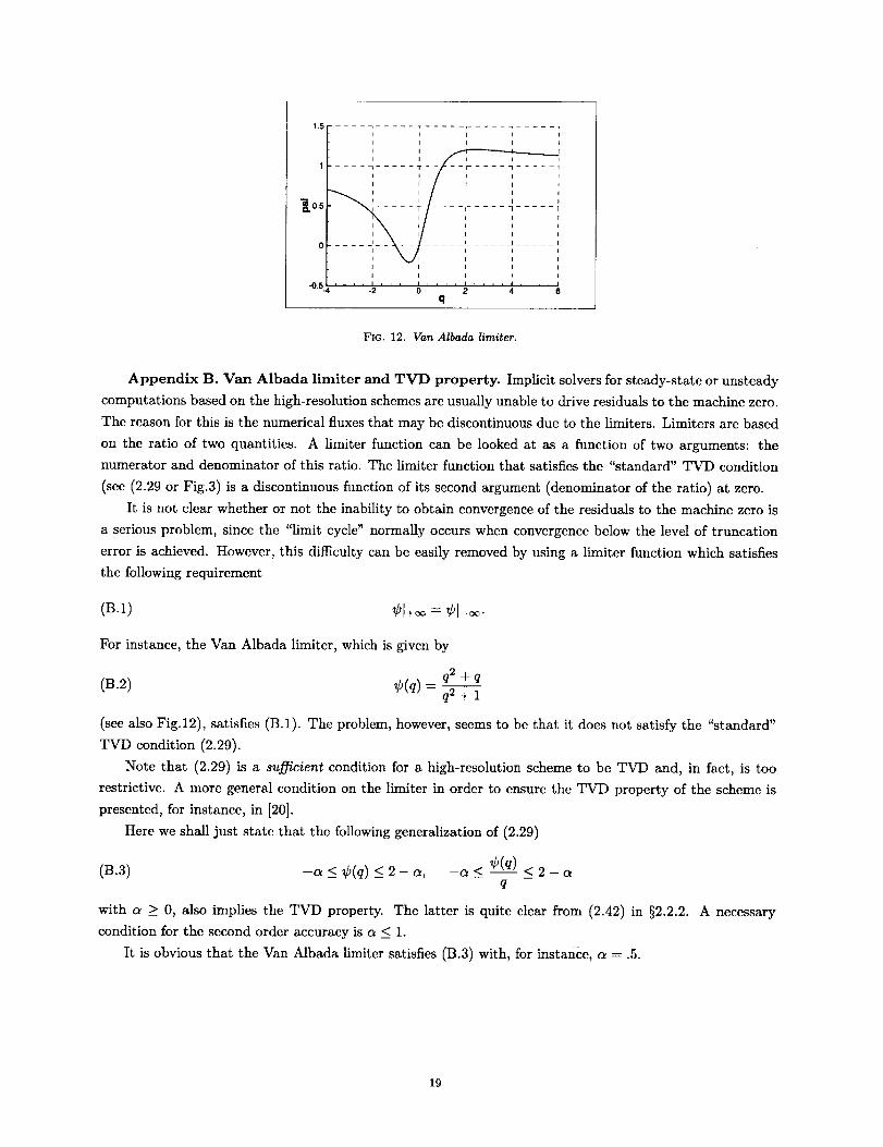
FIG. 12. Van Albada limiter.

Appendix B. Van Albada limiter and TVD property. Implicit solvers for steady-state or unsteady

computations based on the high-resolution schemes are usually unable to drive residuals to the machine zero.

The reason for this is the numerical fluxes that may be discontinuous due to the limiters. Limiters are based

on the ratio of two quantities. A limiter function can be looked at as a function of two arguments: the

numerator and denominator of this ratio. The limiter function that satisfies the "standard" TVD condition

(see (2.29 or Fig.3) is a discontinuous function of its second argument (denominator of the ratio) at zero.

It is not clear whether or not the inability to obtain convergence of the residuals to the machine zero is

a serious problem, since the "limit cycle" normally occurs when convergence below the level of truncation

error is achieved. However, this difficulty can bc easily removed by using a limiter function which satisfies

the following requirement

(B.1) ¢{+_ = ¢1_:¢.

For instance, the Van Albada limiter, which is given by

q2 +q(B.2) ¢(q) -- q2 + 1

(see also Fig.12), satisfies (B.1). The problem, however, seems to be that it does not satisfy the "standard"

TVD condition (2.29).

Note that (2.29) is a sufficient condition for a high-resolution scheme to be TVD and, in fact, is too

restrictive. A more general condition on the limiter in order to ensure the TVD property of the scheme is

presented, for instance, in [20].

Here we shall just state that the following generalization of (2.29)

(B.3) -a < ¢(q) < 2 - or, -a < ¢(q---_)< 2 - c_q

with a > 0, also implies the TVD property. The latter is quite clear from (2.42) in §2.2.2. A necessary

condition for the second order accuracy is cr < 1.

It is obvious that the Van Albada limiter satisfies (]3.3) with, for instance, a = .5.

19

Form ApprovedREPORT DOCUMENTATION PAGE OMBNo.0704-0188

Public repor6ng burden for this collection of information is estimated to average 1 hour per response, including the time for reviewing instructions, searching existing data sources,

gathering and maintaining the data needed, and completing and reviewing the collection of information Send comments regarding this burden est mate or any other aspect of this

collection of information, including suggestions for reducing this burden, to Washington Headquarters Serwces, Dfrectorate for Information Operat=ons and Reports, 1215 Jefferson

I Davis Highway, Suite 1204, Ariington, VA 22202-4302, and to the Office of Management and Budget, Paperwork Reducbon Project (0704-0188), Wash=ngton, DC 20503

1. AGENCY USE ONLY(Leave blank) 2. REPORT DATE 3. REPORT TYPE AND DATES COVERED

October 1998 Contractor Report

4. TITLE AND SUBTITLE 5. FUNDING NUMBERS

A New Time-space Accurate Scheme for Hyperbolic Problems I:Quasi-explicit Case

6. AUTHOR(S)

David Sidilkover

7. PERFORMINGORGANIZATIONNAME(S) AND ADDRESS(ES)Institute for Computer Applications in Science and EngineeringMail Stop 403, NASA Langley Research CenterHampton, VA 23681-2199

9. SPONSORING/MONITORINGAGENCYNAME(S) AND ADDRESS(ES)National Aeronautics and Space AdministrationLangley Research CenterHampton, VA 23681-2199

C NAS1-19480C NAS1-97046WU 505-90-52-01

8. PERFORMING ORGANIZATION

REPORT NUMBER

ICASE Report_NNo. 98-25

10. SPONSORING/MONITORINGAGENCY REPORT NUMBER

NASA/CR-1998-208436ICASE Report No. 98-25

11. SUPPLEMENTARY NOTES

Langley Technical Monitor: Dennis M. BushnellFinal ReportSubmitted to Communications in Applied Analysis

12a. DISTRIBUTION/AVAILABILITY STATEMENT

Unclassified- Unlimited

Subject Category 64Distribution: Nonstandard

Availability: NASA-CASI (301)621-0390

12b. DISTRIBUTION CODE

13. ABSTRACT (Maximum 200 words)

This paper presents a new discretization scheme for hyperbolic systems of conservations laws. It satisfiesthe TVD property and relies on the new high-resolution mechanism which is compatible with the genuinelymultidimensional approach proposed recently. This work can be regarded as a first step towards extending thegenuinely multidimensional approach to unsteady problems. Discontinuity capturing capabilities and accuracy ofthe scheme are verified by a set of numerical tests.

14. SUBJECTTERMSunsteady problems; high-resolution schemes; TVD property

17. SECURITY CLASSIFICATION

OF REPORT

Unclassified

_SN 7540-01-280-5500

18. SECURITY CLASSIFICATIOI_

OF THIS PAGE

Unclassified

19. SECURITY CLASSIFICATION

OF ABSTRACT

1S. NUMBER OF PAGES

24

16. PRICE CODE

A0320. LIMITATION

OF ABSTRACT

Standard Form 298(Rev, 2-89)Prescribed by ANSI Std Z39-18

298-102

_7 I i: