A new submodelling technique for multi-scale finite element
9
Journal of Physics: Conference Series OPEN ACCESS A new submodelling technique for multi-scale finite element computation of electromagnetic fields: Application in bioelectromagnetism To cite this article: K Y Aristovich and S H Khan 2010 J. Phys.: Conf. Ser. 238 012050 View the article online for updates and enhancements. You may also like Hexahedral connection element based on hybrid-stress theory for solid structures D Wu, K Y Sze and S H Lo - Advanced Topics in Computational Partial Differential Equations: Numerical Methods and Diffpack Programming T D Katsaounis - Influence of meshing on thermal effect simulation of laser irradiation Qiudong Qian, Qingtao Wang and Chongxu Wang - Recent citations Application of the finite element submodeling technique in a single point contact and wear problem Cristina Curreli et al - Investigation of optimal parameters for finite element solution of the forward problem in magnetic field tomography based on magnetoencephalography K Y Aristovich et al - This content was downloaded from IP address 191.53.198.139 on 20/01/2022 at 03:30
Transcript of A new submodelling technique for multi-scale finite element

Journal of Physics Conference Series
OPEN ACCESS
A new submodelling technique for multi-scale finiteelement computation of electromagnetic fieldsApplication in bioelectromagnetismTo cite this article K Y Aristovich and S H Khan 2010 J Phys Conf Ser 238 012050
View the article online for updates and enhancements
You may also likeHexahedral connection element based onhybrid-stress theory for solid structuresD Wu K Y Sze and S H Lo
-
Advanced Topics in Computational PartialDifferential Equations Numerical Methodsand Diffpack ProgrammingT D Katsaounis
-
Influence of meshing on thermal effectsimulation of laser irradiationQiudong Qian Qingtao Wang andChongxu Wang
-
Recent citationsApplication of the finite elementsubmodeling technique in a single pointcontact and wear problemCristina Curreli et al
-
Investigation of optimal parameters forfinite element solution of the forwardproblem in magnetic field tomographybased on magnetoencephalographyK Y Aristovich et al
-
This content was downloaded from IP address 19153198139 on 20012022 at 0330
AA new submodelling technique for multi-scale finite element computation of electromagnetic fields application in bioelectromagnetism
K Y Ar istovich and S H KhanSchool of Engineering and Mathematical Sciences City University London Northampton Square London EC1V 0HB UK
E-mail kirillaristovich1cityacuk
Abstract Complex multi-scale Finite Element (FE) analyses always involve high number of elements and therefore require very long time of computations This is caused by the fact that considered effects on smaller scales have greater influences on the whole model and larger scales Thus mesh density should be as high as required by the smallest scale factor New submodelling routine has been developed to sufficiently decrease the time of computationwithout loss of accuracy for the whole solution The presented approach allows manipulation of different mesh sizes on different scales and therefore total optimization of mesh density on each scale and transfer results automatically between the meshes corresponding to respective scales of the whole model Unlike classical submodelling routine the new technique operates with not only transfer of boundary conditions but also with volume results and transfer of forces (current density load in case of electromagnetism) which allows the solution of full Maxwellrsquos equations in FE space The approach was successfully implemented for electromagnetic solution in the forward problem of Magnetic Field Tomography (MFT) based on Magnetoencephalography (MEG) where the scale of one neuron was considered as the smallest and the scale of whole-brain model as the largest The time of computation was reduced about 100 times with the initial requirements of direct computations without submodelling routine of 10 million elements
1 IntroductionDuring the last decade considerable interests in large-scale multiphysics analyses were shown in different areas of research [1-4] Due to increased computational power real-time calculations became possible At the same time a large number of variuous true-scale analyses appeared to be performed Nanotechnology and composite material science were the first fields where complex multi-scale FE simulations were used Then electronics involved such analysis in research and development of various devices Nowadays almost any RampD process requires these analyses to be performed However true-scale simulations still require a lot of computational resources sometimes this becomes critical to the question of actual possibility for these analyses to run at all
The term multi-scale refers to problems where dimensions of different features needed to be considered during simulation of objects are significantly different
Bioelectromagnetism [5] together with some areas of microelectronics is a very scale-sensitive field of research in computational electromagnetics The size of one current source can be significant for a given solution however this size could be on a nanometre scale (eg one neuron one conductive
13th IMEKO TC1-TC7 Joint Symposium IOP PublishingJournal of Physics Conference Series 238 (2010) 012050 doi1010881742-65962381012050
ccopy 2010 Published under licence by IOP Publishing Ltd 1
route or one transistor) with the size of the whole structure being modelled is in centimetres or more (human head PCB)
Submodelling is the common approach which is successfully used in computational mechanics [6]in order to reduce the time of computation with almost no loss of accuracy of the solution Currentlyexisting technique involves the improvement of the solution for example stress concentration valuesat the points of interest and works only in one direction from the large scale (coarse model) to the lowest scale (stress concentrator) Our new approach is designed in order to be implemented in electromagnetic problems where the solution must be improved not only at the points of interest but also in full computational domain
22 Descr iption of Direct Submodelling Routine
Figure 1 Direct Submodelling Routine (SR)
Well-known existing submodelling routines [6] consist of two major steps which can be seen inFigure 1 and it can be described as follows
21 Solution of the coarse problem First the coarse model is analyzed with appropriate boundary conditions During the solution normal mesh convergence analysis must be performed and minimal FE mesh density must be chosen in order to satisfy the required accuracy for the coarse solution The results must be checked in the area outside the external boundaries of the submodel
After the solution is performed all degrees of freedom (DOF) are interpolated on the boundaries of the submodel using element shape functions and then saved
22 Solution of the submodelThe second step is to perform the submodel analysis This analysis is totally independent of the mesh for the coarse model therefore the mesh density of the submodel must be chosen according to new accuracy requirements for this particular region Refined FE mesh could be as dense as it is needed for this solution The boundary conditions are set up as extrapolated solution values obtained from thecoarse model If the main boundary conditions are applicable to the submodel region they should be transferred to the submodel as well
In electromagnetic computations this procedure could be used for static problems with external boundary conditions in order to improve the quantities for the required regions of interest for example for the static volume conduction problems with relatively small inclusions inside the main isotropic domain However this approach does not allow operation with problems where the point of interest is
13th IMEKO TC1-TC7 Joint Symposium IOP PublishingJournal of Physics Conference Series 238 (2010) 012050 doi1010881742-65962381012050
2
outside the object of the lowest scale and this object is significant for the solution eg the current or magnetic field source
33 New Combined Submodelling Routine (CSR)This submodelling routine was developed in order to perform electromagnetic analyses for multi-
scale problems with the electrical or magnetic sources in the smallest scales These problems include quasistatic coupled electromagnetic problem formulations with relatively small size of a magnetic dipole electrical voltage source or electrical current source considered within the computational domain The schematic diagram of the CSR could be seen in Figure 2 The full process could be considered as a combination of the forward and backward submodelling procedures and can be described using the following steps
Figure 22 Combined Submodelling Routine (CSR) applicable to electrical source problems
31 Solution of the course modelThis step is similar to the first step of normal SR with the addition that the submodelling region should be taken around electrical or magnetic sources The interpolation boundaries should be
13th IMEKO TC1-TC7 Joint Symposium IOP PublishingJournal of Physics Conference Series 238 (2010) 012050 doi1010881742-65962381012050
3
relatively far from the source in order to achieve good approximation for the following submodelling solutions The interpolation boundary conditions should also include all degrees of freedom of the solution (magnetic and electric)
32 Solution of the submodelThe submodel solution is performed and the distribution of electric and magnetic fields is obtained in the entire domain The next step depends on the sort of source being considered
33 The coarse model volume interpolationThe entire volume solution of the submodel is then interpolated and transferred as a primary source for the coarse model Only those (electrical or magnetic) degrees of freedom should be transferred into the coarse model of which refer to the primary source In Figure 2 the electrical source is primary so only the electrical DOFs are transferred into the coarse model Note that if all DOFs are interpolated back to the coarse model the solution will not change
34 The coarse model solution with improved sourceAfter the interpolation and transferring is performed the coarse model should be solved with the electric or magnetic field distribution as a primary source instead of the initial source
The approach presented here could be used for multi-source problems such as bioelectromagneticEEG MEG or ECG forward analysis In this case the problem could contain several submodel regions There are also no restrictions on combination of magnetic and electrical sources in one model
The CSR allows to analyze multiple scale problems throughout the application to submodel (for example in case the source is a mixture of a sub-sources) In this case submodelling sub-domain could be also analyzed using CSR
44 Iterative Submodelling Approach (ICSR)
Figure 3 Schematic of the Iterative Combined Submodelling Routine (ICSR)
Iterative Combined Submodelling Routine (ICSR) is developed in order to solve full nonlinear or transient coupled electromagnetic problems with the multi-scale effects As the solution process in case of transient analysis could be nonlinear andor iterative the ICSR operates iteratively in each computational step in time domain The schematic of the ISCR could be seen in Figure 3 The initial step is the same as CSR and then the solution is improved in each iteration until it converges
13th IMEKO TC1-TC7 Joint Symposium IOP PublishingJournal of Physics Conference Series 238 (2010) 012050 doi1010881742-65962381012050
4
This procedure could be also used in a static analysis with mesh convergence criteria to be run inthe second step (second box in Figure 3) In this work the performance of ICSR was not tested due to specific areas of application Transient multi-scale analysis is a relatively new field of research and further investigation is required in order to obtain ICSR parameters and optimize its performance for individual cases It is believed that for a given particular problem new optimization analyses routine needs to be performed
Most bioelectric problems are considered quasistatic with a good level of approximation The frequencies of the signal in biological structures are not higher than 1MHz So transient effects have no influence on the total solution [5]
55 Results of Simulation and Performance AnalysisIn this work the CSR was implemented and tested for solving one of the most complex biomagnetic forward problems The solution of the forward problem in magnetic field tomography (MFT) based on magnetoencephalography (MEG) constitutes the prime topic of research conducted by the authors
51 Solution of the forward problem in MFT based on MEGThe formulation of the problem can be found in a wide range of literature [7-9] In short the forwardproblem comprises the computation of magnetic field distribution around the human head from known currents in the brain caused by cognitive activity More precisely this electrical activity is caused by an action potential distribution along the neuronal axon This effect could be modelled as a voltage difference applied to a small segment of an axon at each time frame [10] Since action potential propagates with relatively small velocity of 10 ms the problem could be considered as quasistatic Calculations at a given iterative time step can be considered independent of successive time steps andtherefore CSR could be applied in order to significantly reduce computational time
Here we consider a full realistic 3D finite element model of the human brain described earlier in paper [11] The parameters of such a model are given in Table 1
The geometric and physical parameters of the model were obtained from MRI slices resulting from a whole-brain scan In terms of finite elements the model considered a complex anisotropic conductor with realistic tissue properties obtained from DTMRI scan of the same subject A model with fine mesh was considered first in order to validate results of CSR Around 10m FE elements were chosen for the fine model in order to satisfy the mesh convergence criteria of 1
For the coarse model a relatively low mesh density with around 800k FE elements was used This satisfies the mesh convergence criteria for the brain model without any neuronal source inside For the submodel 300k elements were found to be adequate to satisfy the accuracy requirements
In Figure 4 and Figure 5 the outline of the brain is shown together with the boundaries of the submodelling region and neuronal source The neuronal source is considered as an action potential with voltage difference of 50mV The thickness of the neuronal path is 05mm which is not realistic in order to test the effect of CSR on the solution It is obvious that the efficiency of the use of CSR is increased with the increase in the difference in scale so for realistic micron-thickness of neuronal axons the estimated computation time will decrease even further
52 Simulation results and comparisonThe computational set-up was made and then the quasistatic Maxwellrsquos equations were solved in the FE domain The results were obtained for both the fine mesh and the CSR model and then compared
Figure 6 shows the distribution of magnetic flux density on the detector surface around the head (points of interest for the solution) It can be seen that the coarse model on its own gives less accurateresults However the application of CSR vastly improves the accuracy and the results are almost the same (maximum error of 5) as for the fine model
13th IMEKO TC1-TC7 Joint Symposium IOP PublishingJournal of Physics Conference Series 238 (2010) 012050 doi1010881742-65962381012050
5
TTable 11 Parameters of FE models and solution
PParameter VValuedescr iptionGeometry of the model
Realistic geometry ob-tained from MRI scan
Material Properties
Realistic anisotropic tensor conductivity distribution obtained from DTMRI scanpermeability of the air
Solution Quasistatic single stepcoupled electromagnetic problem (magnetic vector potential AA and electric potential V)
Neuronal source
Part of neuronal axon with voltage difference of 50 mV applied to ends of a segmentthickness of the axon is 05 mm
Number of elements
Fine model ndash 10mCoarse model ndash 800kSubmodel ndash 300k
Figure 4 Outline of the brain model showingpositions of the submodelling region and the neuronal source
Figure 5 Comparison of meshes for submodelling region and the neuronal source coarse model (left) and submodel (right)
Figure 7 shows and improvement of current density distribution in the solution with the application of CSR This distribution has been found to be the main reason for adequate magnetic field computation and it has been computed more accurately using the submodelling technique which results in the improvement on the solution obtained by the coarse model
The magnetic flux density isosurfaces (Figure 8) also show less accurate spatial magnetic field distribution in the coarse model which has been improved in the CSR model (note the difference in the top configuration of the isosurface)
Average resulting CSR error for this case was calculated using the equation
(1)
where and are the values of magnetic field flux density at the nodes on the detector surface N is the total number of nodes on this surface Overall comparison results are summarized in
Table 2 where solution times of for both the fine and CSR models are presented
6 ConclusionsThe Combined Submodelling Routine (CSR) and Iterative Combined Submodelling Routine (ICSR) were developed for multi-scale problems in order to reduce the computational time with minimum losssolution accuracy
13th IMEKO TC1-TC7 Joint Symposium IOP PublishingJournal of Physics Conference Series 238 (2010) 012050 doi1010881742-65962381012050
6
These routines can have a wide range of application especially in bioelectromagnetic problems where in many cases it is important to consider multiple scales The CSR was tested for the solution of the forward problem in MFT based on MEG Comparison of results between the solutions from initial fine FE model with appropriate mesh density required for direct analysis and CSR applied to the same
Figure 6 Results of simulation comparison among results from initial coarse model (left) fine model (middle) and CSR solution (right) Rows represent top and side views respectively
Figure 7 Current density distribution inside the submodelling region of the coarse model Direct coarse model solution (left) and solution after application of CSR (right)
Figure 8 Magnetic flux density isosurface plots for coarse model (left) and with submodelling approach (right)
13th IMEKO TC1-TC7 Joint Symposium IOP PublishingJournal of Physics Conference Series 238 (2010) 012050 doi1010881742-65962381012050
7
problem highlighted the ability of CSR to significantly reduce computational time (approximately 100 times) with almost no loss of solution accuracy Average error of the CSR solution has been found to be 03 for the chosen size of submodelling region
Further analyses carried out show that CSR can decrease computational time even more for thosecases where the difference between geometric dimensions is higher
Future investigation is planned in order to evaluate errors and optimal parameters for ICSR which is also applicable to transient and nonlinear electromagnetic multi-scale problems for example in microelectronics
Table 2 Comparison between fine model and CSR solutionsPParameter FFine model CCSR model
Number of elements 10m 08m (coarse) + 03m (submodel)
Maximum magnetic flux density 339 10-11 T 319 10-11 T
Maximum error of the CSR solution 5
Average error of the CSR solution computed by equation (1) e
003
Solution time 168 hours 15 hours
77 References[1] Garcia A and Durand C 2009 Bioengineering Principles methodologies and applications
(Hauppauge NY Nova Science Publishers)[2] Pozrikidis C 2010 Computational hydrodynamics of capsules and biological cells (Boca Raton
Chapman amp HallCRC)[3] Fishwick P A 2007 Handbook of dynamic system modeling (Boca Raton Chapman amp
HallCRC)[4] Leondes C T 1999 Structural dynamic systems computational techniques and optimization
Nonlinear techniques (Amsterdam Gordon and Breach Science Publishers)[5] He B 2004 Modeling and imaging of bioelectrical activity Principles and applications (New
York Kluwer AcademicPlenum Publishers)[6] ANSYS I 2010 Submodelling In Release 110 Documentation for Ansys[7] Ellenrieder N V Muravchik C H and Nehorai A 2005 MEG forward problem formulation using
equivalent surface current densities IEEE transactions on biomedical engineering 52 8[8] Gencer N G and Tanzer I O 1999 Forward problem solution of electromagnetic source imaging
using a new bem formulation with high-order elements Phys Med Biol 44 2275-87[9] Hamalainen M Hari R Ilmoniemi R J Knuutila J and Lounasmaa O V 1993
Magnetoencephalography-theory instrumentation and applications to noninvasive studies of the working human brain Rev Modern Phys 65 84
[10] Bear M F Connors B W and Paradiso M A 2007 Neuroscience Exploring the brain(Baltimore Md Lippincott Williams amp Wilkins)
[11] Khan S H Aristovich K Y and Borovkov A I 2009 Solution of the forward problem in magnetic-field tomography (MFT) based on magnetoencephalography (MEG) IEEE transactions on magnetics 45 4
13th IMEKO TC1-TC7 Joint Symposium IOP PublishingJournal of Physics Conference Series 238 (2010) 012050 doi1010881742-65962381012050
8
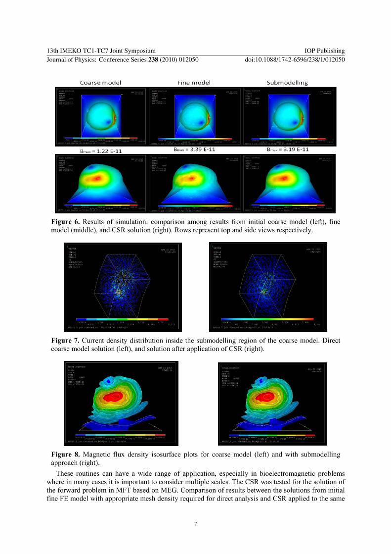