A NEW STICKY PARTICLE METHOD FOR PRESSURELESS GAS DYNAMICS et al... · Vol. 45, No. 6, pp. 2408 ......
34
Copyright © by SIAM. Unauthorized reproduction of this article is prohibited. SIAM J. NUMER. ANAL. c 2007 Society for Industrial and Applied Mathematics Vol. 45, No. 6, pp. 2408–2441 A NEW STICKY PARTICLE METHOD FOR PRESSURELESS GAS DYNAMICS ∗ ALINA CHERTOCK † , ALEXANDER KURGANOV ‡ , AND YURII RYKOV § Abstract. We first present a new sticky particle method for the system of pressureless gas dynamics. The method is based on the idea of sticky particles, which seems to work perfectly well for the models with point mass concentrations and strong singularity formations. In this method, the solution is sought in the form of a linear combination of δ-functions, whose positions and coefficients represent locations, masses, and momenta of the particles, respectively. The locations of the particles are then evolved in time according to a system of ODEs, obtained from a weak formulation of the system of PDEs. The particle velocities are approximated in a special way using global conservative piecewise polynomial reconstruction technique over an auxiliary Cartesian mesh. This velocities correction procedure leads to a desired interaction between the particles and hence to clustering of particles at the singularities followed by the merger of the clustered particles into a new particle located at their center of mass. The proposed sticky particle method is then analytically studied. We show that our particle approximation satisfies the original system of pressureless gas dynamics in a weak sense, but only within a certain residual, which is rigorously estimated. We also explain why the relevant errors should diminish as the total number of particles increases. Finally, we numerically test our new sticky particle method on a variety of one- and two-dimensional problems as well as compare the obtained results with those computed by a high-resolution finite-volume scheme. Our simulations demonstrate the superiority of the results obtained by the sticky particle method that accurately tracks the evolution of developing discontinuities and does not smear the developing δ-shocks. Key words. nonstrictly hyperbolic systems of conservation laws, pressureless gas dynamics, mass concentration, strong singularities, δ-shock, sticky particle method AMS subject classifications. 65M25, 65M12, 35L65, 35L67 DOI. 10.1137/050644124 1. Introduction. We consider the Euler equations of pressureless gas dynamics: (1.1) w t + ∇ x · (u ⊗ w)= 0. Here, x := (x,y,...) is an n-dimensional vector of spatial variables, u := (u,v,...) is the corresponding velocity vector, and w ≡ (w 1 ,w 2 ,w 3 ,...) T := (ρ, ρu, ρv, . . .) T is the (n + 1)-dimensional vector of unknown function, where ρ is the density. This system arises in the modeling of the formation of large-scale structures in the universe [24]. It can be formally obtained as the limit of the isotropic Euler equations of gas dynamics as pressure tends to zero or as the macroscopic limit of a Boltzmann equation when the Maxwellian has zero temperature. ∗ Received by the editors November 2, 2005; accepted for publication (in revised form) April 6, 2007; published electronically November 21, 2007. http://www.siam.org/journals/sinum/45-6/64412.html † Department of Mathematics, North Carolina State University, Raleigh, NC 27695 (chertock@ math.ncsu.edu). This author’s work was supported in part by NSF grant DMS-0410023. ‡ Mathematics Department, Tulane University, New Orleans, LA 70118, and Department of Math- ematics, University of Michigan, Ann Arbor, MI 48109 ([email protected]). This author’s work was supported in part by NSF grants DMS-0310585 and DMS-0610430. § Keldysh Institute of Applied Mathematics, Russian Academy of Sciences, 125047 Moscow, Russia ([email protected]). This author’s work was supported in part by Russian Foundation for Basic Research grant 030100189 and by Program 01 of the Division of Mathematical Sciences of the Russian Academy of Sciences. 2408
Transcript of A NEW STICKY PARTICLE METHOD FOR PRESSURELESS GAS DYNAMICS et al... · Vol. 45, No. 6, pp. 2408 ......

Copyright © by SIAM. Unauthorized reproduction of this article is prohibited.
SIAM J. NUMER. ANAL. c© 2007 Society for Industrial and Applied MathematicsVol. 45, No. 6, pp. 2408–2441
A NEW STICKY PARTICLE METHOD FOR PRESSURELESS GASDYNAMICS∗
ALINA CHERTOCK† , ALEXANDER KURGANOV‡ , AND YURII RYKOV§
Abstract. We first present a new sticky particle method for the system of pressureless gasdynamics. The method is based on the idea of sticky particles, which seems to work perfectly wellfor the models with point mass concentrations and strong singularity formations. In this method, thesolution is sought in the form of a linear combination of δ-functions, whose positions and coefficientsrepresent locations, masses, and momenta of the particles, respectively. The locations of the particlesare then evolved in time according to a system of ODEs, obtained from a weak formulation of thesystem of PDEs. The particle velocities are approximated in a special way using global conservativepiecewise polynomial reconstruction technique over an auxiliary Cartesian mesh. This velocitiescorrection procedure leads to a desired interaction between the particles and hence to clusteringof particles at the singularities followed by the merger of the clustered particles into a new particlelocated at their center of mass. The proposed sticky particle method is then analytically studied. Weshow that our particle approximation satisfies the original system of pressureless gas dynamics in aweak sense, but only within a certain residual, which is rigorously estimated. We also explain why therelevant errors should diminish as the total number of particles increases. Finally, we numerically testour new sticky particle method on a variety of one- and two-dimensional problems as well as comparethe obtained results with those computed by a high-resolution finite-volume scheme. Our simulationsdemonstrate the superiority of the results obtained by the sticky particle method that accuratelytracks the evolution of developing discontinuities and does not smear the developing δ-shocks.
Key words. nonstrictly hyperbolic systems of conservation laws, pressureless gas dynamics,mass concentration, strong singularities, δ-shock, sticky particle method
AMS subject classifications. 65M25, 65M12, 35L65, 35L67
DOI. 10.1137/050644124
1. Introduction. We consider the Euler equations of pressureless gas dynamics:
(1.1) wt + ∇x · (u ⊗ w) = 0.
Here, x := (x, y, . . .) is an n-dimensional vector of spatial variables, u := (u, v, . . .)is the corresponding velocity vector, and w ≡ (w1, w2, w3, . . .)T := (ρ, ρu, ρv, . . .)T isthe (n + 1)-dimensional vector of unknown function, where ρ is the density.
This system arises in the modeling of the formation of large-scale structures in theuniverse [24]. It can be formally obtained as the limit of the isotropic Euler equationsof gas dynamics as pressure tends to zero or as the macroscopic limit of a Boltzmannequation when the Maxwellian has zero temperature.
∗Received by the editors November 2, 2005; accepted for publication (in revised form) April 6,2007; published electronically November 21, 2007.
http://www.siam.org/journals/sinum/45-6/64412.html†Department of Mathematics, North Carolina State University, Raleigh, NC 27695 (chertock@
math.ncsu.edu). This author’s work was supported in part by NSF grant DMS-0410023.‡Mathematics Department, Tulane University, New Orleans, LA 70118, and Department of Math-
ematics, University of Michigan, Ann Arbor, MI 48109 ([email protected]). This author’swork was supported in part by NSF grants DMS-0310585 and DMS-0610430.
§Keldysh Institute of Applied Mathematics, Russian Academy of Sciences, 125047 Moscow, Russia([email protected]). This author’s work was supported in part by Russian Foundation for BasicResearch grant 030100189 and by Program 01 of the Division of Mathematical Sciences of the RussianAcademy of Sciences.
2408

Copyright © by SIAM. Unauthorized reproduction of this article is prohibited.
PARTICLE METHOD FOR PRESSURELESS GAS DYNAMICS 2409
Even in the simplest one-dimensional (1-D) case, the system (1.1), which can berewritten as
(1.2)
{ρt + (ρu)x = 0,(ρu)t + (ρu2)x = 0,
is mathematically challenging since it is nonstrictly hyperbolic and its Jacobian is notdiagonalizable. For smooth solutions, the system (1.2) is equivalent to
ρt + (ρu)x = 0,(1.3)
ut + uux = 0.(1.4)
Notice that (1.4) is the inviscid Burgers equation, which is, in fact, decoupled from(1.3). It is well known that the solution of the initial-value problem associated with(1.4), as long as it stays smooth, can be easily obtained by the method of charac-teristics. The density ρ can then be determined from (1.3), which becomes a lineartransport equation. However, if the initial velocity u(x, 0) is not monotone increas-ing, the characteristics will intersect within a finite time, and the solution will loseits initial smoothness, and thus it must be understood in a weak sense. As in thegeneral theory of weak solutions of hyperbolic systems of conservation laws, one hasto introduce discontinuity lines. Let x = ξ(t) be such a line and assume that thesolution accepts finite values u± := u(ξ(t) ± 0, t) and ρ± := ρ(ξ(t) ± 0, t) from bothsides of discontinuity. The jumps then must satisfy the Rankine–Hugoniot conditions,namely, {
ξ′(t) (ρ+ − ρ−) = ρ+u+ − ρ−u−,
ξ′(t) (ρ+u+ − ρ−u−) = ρ+ (u+)2 − ρ− (u−)
2.
After eliminating ξ′ from this system, one obtains ρ+ρ− (u+ − u−)2
= 0, which impliesu+ = u−. Therefore, in order to support the shock discontinuity in the velocity field,the density must have a stronger (than a shock) singularity at x = ξ′(t). Since in theBurgers equation, the characteristic lines impinge each other and thus, as part of thesystem (1.2), cause a mass concentration at the velocity discontinuity line, resultingin the formation of a δ-type singularity in the density field there.
The two-dimensional (2-D) version of (1.1) reads as
(1.5)
⎧⎨⎩ρt + (ρu)x + (ρv)y = 0,(ρu)t + (ρu2)x + (ρuv)y = 0,(ρv)t + (ρuv)x + (ρv2)y = 0.
Compared to the 1-D case, solutions of the 2-D system have a similar but essentiallymore sophisticated mechanism of singularities formation due to the dimensionalityfactor: strong singularities may now be formed either along surfaces or at separatepoints (we expect that in the three space dimensions the situation is even more com-plex). The system (1.5) has been intensively studied at the theoretical level (see, e.g.,[2, 4, 6, 7, 8, 20, 21]). However, no more or less complete analytical results concerningthe existence and uniqueness of solutions in the 2-D case are available. This is pri-marily related to the difficulties in the theoretical description of the collision of 2-Dshocks. (See section 3.2 for an extensive numerical study of this phenomenon.)
Formation and further evolution of singular shocks, their interactions as well asthe emergence of vacuum states, make development of numerical methods for the

Copyright © by SIAM. Unauthorized reproduction of this article is prohibited.
2410 A. CHERTOCK, A. KURGANOV, AND YU. RYKOV
system (1.1) a challenging problem. A numerical method based on the movement of asystem of particles was introduced in [19]. Several finite-volume [17], kinetic [2, 3, 5],and relaxation [1] methods have been recently proposed. These methods are able toreasonably accurately capture δ-shocks, but their applicability is rather limited; forexample, most of these methods do not work well for problems where the velocitieschange sign in regions where the density varies smoothly [17].
We develop a simple, efficient, and low-dissipative sticky particle method for pres-sureless gas dynamics. The derivation of our method is based on a weak formulation ofthe system (1.5) and can be viewed as a practical implementation of the sticky particlemethod from [4]. We first approximate w by a collection of N particles, located at(xN
i (t), yNi (t)), i = 1, . . . , N , at time t, and carrying fixed masses and momenta. Theparticle locations are then evolved according to the corresponding system of ODEs,derived by plugging the particle approximation into a weak form of (1.1). In order toprevent the situation, in which approaching particles simply pass by each other with-out any interaction (such an undesirable situation is obviously impossible in the 1-Dcase, but is almost unavoidable in the 2-D case), we divide the computational domaininto a set of auxiliary cells and compute the total mass and momenta in each cell.The particle velocities are then approximated using the global conservative piecewisepolynomial interpolants of ρ, ρu, and ρv, constructed over an auxiliary Cartesianmesh. This way an interaction of all particles located in the same cell is guaranteed.When the particles get even closer to each other, we unite them into a new particle,located at the center of mass of the original clustered particles. The mass (momen-tum) of the new particle is simply the sum of the masses (corresponding momenta) ofthe replaced particles, and the velocities of the new particle are uniquely determinedfrom the conservation requirements. This particle merger procedure results in massconcentration, which is an essential property of pressureless gases.
We would like to note that our 2-D sticky particle method can be extended toany number of space dimensions in a rather straightforward manner. In this paper,we restrict our consideration to the 1-D and 2-D cases only, since, to the best of ourknowledge, no analytical results on three-dimensional (3-D) pressureless gas dynamicssystem are available, and it is therefore hard to set up convincing 3-D numericalexperiments.
We test our method on a number of 1-D and 2-D numerical examples, in which wecompare the results obtained by the new (nondissipative) sticky particle method andby the (dissipative) second-order central-upwind scheme from [11]. The latter schemeis a high-resolution Godunov-type finite-volume method that belongs to a family ofcentral schemes, which may serve as “black-box” solvers for multidimensional hy-perbolic systems of conservation laws. The prototype of modern central schemes isthe first-order Lax–Friedrichs scheme [9, 16], which is the most universal method forsolving (multidimensional systems of) time-dependent PDEs. However, its excessivenumerical dissipation prevents sharp resolution and therefore in practice one has touse higher-order schemes. The first high-resolution nonoscillatory central scheme—thesecond-order Nessyahu–Tadmor scheme—was proposed in [18]. The amount of numer-ical dissipation present in projection-evolution central schemes was further reducedby incorporating some more upwinding information on local speeds of propagationinto the evolution step [12, 14] (the resulting schemes thus have been referred to ascentral-upwind schemes) and, more recently, by enhancing the accuracy of the pro-jection step [11, 13]. We note that the only upwinding information required by thecentral-upwind schemes is the eigenvalues of the Jacobians, and therefore applicationof these schemes to nonstrictly hyperbolic systems like (1.5) is straightforward.

Copyright © by SIAM. Unauthorized reproduction of this article is prohibited.
PARTICLE METHOD FOR PRESSURELESS GAS DYNAMICS 2411
The paper is organized as follows. We start in section 2 by introducing the newsticky particle method for the system (1.5). We then describe, in section 2.1, thevelocity correction procedure and, in section 2.2, an algorithm of the unification ofclustering particles. The main analytical result in section 2.3 is Theorem 2.1, wherewe show that even though our particle solution fails to satisfy (1.1) in a weak sensedefined in [21], the relevant errors can be rigorously estimated. We then provide aheuristic justification why these errors tend to zero as N → ∞. We conclude insection 3 with several 1-D and 2-D numerical examples and demonstrate that the newmethod accurately tracks the evolution of developing discontinuities. We also comparesolutions computed by the sticky particle method with the corresponding solutionscomputed using the second-order semidiscrete central-upwind scheme, developed in[11, 12, 14]. A brief description of the central-upwind scheme for the pressureless gasdynamics system (1.5) is provided in Appendix A.
2. Derivation of the sticky particle method. We consider the system (1.1)subject to the compactly supported (or periodic) initial data,
(2.1) w(x, 0) ≡ (ρ(x, 0), ρu(x, 0), ρv(x, 0))T , x := (x, y)T ,
and look for the solution of the initial-value problem (1.1), (2.1) in the particle form,
(2.2) wN(x, t) =
N∑i=1
αi(t)δ(x − xNi (t)), xN
i := (xNi , yNi )T, αi = (mi,miui,mivi)
T .
Here, N is a total number of particles, xNi (t) is the location of the ith particle at time
t, and mi,miui, and mivi are its mass, the x-, and the y-momenta, respectively.In order to study the particle time evolution, we plug (2.2) into the weak formu-
lation of the system (1.1),
(2.3)
∫ ∞
0
∫∫R2
{wN · [ϕt + uϕx + vϕy]
}dxdt−
∫∫R2
wN (x, 0) ·ϕ(x, 0) dx = 0,
where ϕ is an arbitrary C10 test function. As a result, (2.3) reduces to
(2.4)N∑i=1
∫ ∞
0
αi(t) ·{ϕt + uϕx + vϕy
} ∣∣∣∣∣(x,t)=(xN
i (t),t)
dt−N∑i=1
αi(0) ·ϕ(xNi (0), 0) = 0,
which should be satisfied for any ϕ. Evolving particle locations according to thefollowing system of ODEs:
(2.5)dxN
i (t)
dt= u(xN
i (t), t),dyNi (t)
dt= v(xN
i (t), t), i = 1, . . . , N,
and integrating by parts, we rewrite (2.4) as
N∑i=1
∫ ∞
0
dαi(t)
dt·ϕ(xN
i (t), t) dt = 0.
The last equation implies
(2.6)dαi(t)
dt= 0, i = 1, . . . , N,

Copyright © by SIAM. Unauthorized reproduction of this article is prohibited.
2412 A. CHERTOCK, A. KURGANOV, AND YU. RYKOV
that is, the particle weights remain constant in time. Thus, the weights can bedetermined from the initial conditions, for instance, in the following manner. Wedivide the computational domain Ω into N subdomains Ωi, i = 1, . . . , N , and placean ith particle with
αi :=
∫∫Ωi
w(x, 0) dx
into the center of Ωi, denoted by xNi (0) ≡ (xN
i (0), yNi (0)), which will serve as initialdata for the ODE system (2.5).
2.1. Particle velocities. In order to be able to solve the system of ODEs (2.5),one would need to recover the particle velocities at any given time moment. Thesimplest (and the least dissipative) way to compute the velocities is to divide thecorresponding particle momenta by its mass, that is, by taking
(2.7) ui ≡ u(xNi (t), t) :=
miui
mi, vi ≡ v(xN
i (t), t) :=mivimi
.
In fact, this means that every particle travels with constant velocity until it collideswith another particle (see section 2.2). This approach can be rigorously justifiedthrough the weak formulation (2.3) and it seems to work perfectly in the 1-D case,in which collision of approaching particles is unavoidable. However, in the 2-D case,the probability of collision of two particles approaching the same singularity curveis zero unless a special symmetry in initial particle locations has been imposed (seeExample 5 in section 3.2).
We propose an alternative way of particle velocities reconstruction, which is in-dependent of an initial placement of particles. Our approach is based on a globalpiecewise polynomial reconstruction technique, which is widely used in finite-volumeframework (see Appendix A and the references therein). To adopt this technique to amesh-free particle method we introduce an auxiliary Cartesian grid (which may varyin time). The grid should be adapted to the particle distribution so that the numberof particles in every cell is about the same. In our numerical experiments, we haveused the simplest strategy: we have adapted the auxiliary grid to the initial (uniform)particle distribution only by taking the size of the cells to be twice larger than thedistance between the particles. A more sophisticated adaptation strategy may lead tomore accurate results, but its optimization may substantially increase the complexityof the proposed sticky particle method.
Taking a simple uniform auxiliary grid, xj ≡ jΔx, yk ≡ kΔy, we first computethe cell averages of the conserved quantities at time t,
(2.8) wj,k(t) =1
ΔxΔy
∑i:xN
i (t)∈Ij,k
αi, Ij,k = [xj− 12, xj+ 1
2] × [yk− 1
2, yk+ 1
2].
Using these cell averages, we then reconstruct a nonoscillatory piecewise polynomialinterpolant of an appropriate order of accuracy, denoted by
w(x, t) := (w1(x, t), w2(x, t), w3(x, t))T ,
which is used to compute the particle velocities,
(2.9) ui :=w2(xN
i (t), t)
w1(xNi (t), t)
, vi :=w3(xN
i (t), t)
w1(xNi (t), t)
.

Copyright © by SIAM. Unauthorized reproduction of this article is prohibited.
PARTICLE METHOD FOR PRESSURELESS GAS DYNAMICS 2413
Notice that in order to ensure that no mass (momentum) is artificially lost (created)at this step, the reconstruction must be performed in a conservative manner, namely,one should guarantee that ∑
i:xNi (t)∈Ij,k
w(xNi (t), t) = wj,k(t).
We achieve the conservation (in fact, while the mass is conserved exactly, only ap-proximate momentum conservation is guaranteed; see the computation in section 2.3)by taking w to be a second-order accurate piecewise linear reconstruction centered atthe center of mass of the particles located in the Ij,k cell,
w(x, y, t) = wj,k + (sx)j,k(x− xCMj,k (t))
+ (sy)j,k(y − yCMj,k (t)) for (x, y) ∈ Ij,k,(2.10)
where the coordinates of the center of mass are
(2.11) xCMj,k (t) :=
∑i:xN
i (t)∈Ij,k
mixNi (t)
∑i:xN
i (t)∈Ij,k
mi
, yCMj,k (t) :=
∑i:xN
i (t)∈Ij,k
miyNi (t)
∑i:xN
i (t)∈Ij,k
mi
,
and the slopes (sx)j,k and (sy)j,k are (at least) first-order approximations of the
derivatives wx(xCMj,k (t), yCM
j,k (t)) and wy(xCMj,k (t), yCM
j,k (t)), respectively.
Finally, in order to ensure a nonoscillatory nature of the reconstruction (2.10),the slopes (sx)j,k and (sy)j,k should be computed using a nonlinear limiter. In ournumerical experiments, we have used the minmod limiter applied in the following way.
Let us take, for example, the first component of w (density) and consider the fourplanes, denoted by πNE
j,k , πNWj,k , πSE
j,k, πSWj,k , that pass through the following four triplets
of points:
(2.12)
πNEj,k :
{(xCM
j,k , yCMj,k , w1
j,k), (xCMj,k+1, y
CMj,k+1, w
1j,k+1), (xCM
j+1,k, yCMj+1,k, w
1j+1,k)
},
πNWj,k :
{(xCM
j,k , yCMj,k , w1
j,k), (xCMj,k+1, y
CMj,k+1, w
1j,k+1), (xCM
j−1,k, yCMj−1,k, w
1j−1,k)
},
πSEj,k :
{(xCM
j,k , yCMj,k , w1
j,k), (xCMj,k−1, y
CMj,k−1, w
1j,k−1), (xCM
j+1,k, yCMj+1,k, w
1j+1,k)
},
πSWj,k :
{(xCM
j,k , yCMj,k , w1
j,k), (xCMj,k−1, y
CMj,k−1, w
1j,k−1), (xCM
j−1,k, yCMj−1,k, w
1j−1,k)
}(the dependence of {xCM
j,k } and {yCMj,k } on t has been omitted here for briefness). We
then denote the gradients of these planes by ((πx)NEj,k , (πy)
NEj,k )T , ((πx)NW
j,k , (πy)NWj,k )T ,
etc., and take the first component of the slopes in (2.10) to be
(2.13)
(s1x)j,k = minmod
((πx)NE
j,k , (πx)NWj,k , (πx)SE
j,k, (πx)SWj,k
),
(s1y)j,k = minmod
((πy)
NEj,k , (πy)
NWj,k , (πy)
SEj,k, (πy)
SWj,k
),

Copyright © by SIAM. Unauthorized reproduction of this article is prohibited.
2414 A. CHERTOCK, A. KURGANOV, AND YU. RYKOV
where the minmod function is defined by
(2.14) minmod(c1, c2, . . .) :=
⎧⎨⎩min(c1, c2, . . .) if ci > 0 ∀i,max(c1, c2, . . .) if ci < 0 ∀i,0 otherwise.
The reconstructions for the other two fields of w (momenta) are obtained in a similarway.
Remarks.1. It may happen that one of the planes in (2.12) is perpendicular to the (x, y)-
plane or is not uniquely determined. Then this plane is not taken into account,and its gradient is excluded from the formulae for the slopes in (2.13).
2. As was mentioned in section 1, our velocity recovery procedure ensures thatthere is an interaction between the particles, located inside the same auxiliarygrid cell. As is illustrated in our numerical experiments (see section 3.2), thisleads to the desired clustering of particles at the singularities.
2.2. Unification of clustering particles. A major drawback of particle meth-ods is that, in general, their resolution and efficiency significantly deteriorate whentoo many particles cluster near the same point at the singularity. To prevent such anundesired situation, we unite clustering particles according to the following algorithm.We choose a certain critical distance dcr and as soon as the distance between any twoparticles gets smaller than the critical distance, we unite them into a new “heavier”particle.
Let us assume that at some time t, the distance between the ith and the jthparticles, |xi(t)−xj(t)|, is smaller than dcr. We then replace these two particles witha new one of the following total mass and momenta:
(2.15) αnew = αi + αj ,
located at the center of mass of the replaced particles, namely,
(2.16) xNnew =
mixNi + mjx
Nj
mi + mj.
The velocities of the new particle are determined according to the procedure in sec-tion 2.1. After completing the replacement process (2.15)–(2.16), we check whetherany other two particles are to be united, and if not, the remaining set of particles isfurther evolved in time according to (2.2), (2.5), (2.9) until another particle clusteringoccurs. Then, the unification procedure is repeated, and so forth.
Remark. The critical distance dcr should be chosen experimentally. In all ournumerical examples, except for Example 4, this distance was taken a quarter of aminimal initial distance between the particles (note that the initial distribution ofparticles is rather uniform in every numerical example below). In Example 4, dcr wasmade proportional to the size of the shrinking support of the solution.
We would also like to stress that our numerical experiments clearly indicate thatthe presented sticky particle method does not seem to be sensitive to the choice of dcr.
2.3. On convergence of the sticky particle method. In previous sections,a sequence of approximate solutions {wN}∞N=1 of the system (1.1) for a fixed timeinterval [0, T ] has been constructed based on the dynamics of moving particles. Inthis section, we show that the measures wN do not satisfy (1.1) in a weak sense.

Copyright © by SIAM. Unauthorized reproduction of this article is prohibited.
PARTICLE METHOD FOR PRESSURELESS GAS DYNAMICS 2415
Nevertheless, in Theorem 2.1, we obtain rigorous estimates for relevant errors andfurther discuss the heuristic justification why these errors tend to zero as N → ∞.
In order to exactly formulate the theorem, let us first describe the interactions ofmoving particles in detail. Consider a time interval [t1, t2] ⊂ [0, T ], some number pof moving particles, and a time moment t0 such that the particles evolve accordingto the ODE system (2.5)–(2.6) for t ∈ [t1, t0) and t ∈ (t0, t2], while at time t0 theparticles either coalesce (Case I) or change the velocities according to (2.9) (Case II).
For the considered group of p particles, P, with the total mass
M :=∑i∈P
mi,
we introduce the following notation.• Prior to t = t0 we denote byαi = (mi,miui,mivi)
T: weights of the particles,
(xi(t), yi(t)): their locations at time t < t0,(x0
i , y0i ) = (xi(t0), yi(t0)): final locations of the particles at time t = t0.
• At t = t0 the considered p particles either− coalesce (Case I) and then we denote byα = (M,MU,MV ): weights of the newly formed particle of mass M ,
U =
∑i∈P miui∑i∈P mi
and V =
∑i∈P mivi∑i∈P mi
: its x- and y-velocities,
(X0, Y0) = (X(t0), Y (t0)): its initial position at time t = t0,(X(t), Y (t)): its location at time t > t0;or− undergo the velocities correction (Case II) and then we denote by
αi = (mi,miui,mivi)T: new weights of the original p particles,
(xi(t), yi(t)): their locations, which are not instantaneously affected by thevelocities correction procedure and thus change continuously.
We also denote by(xCM(t), yCM(t)
)the location of the center of mass of the
considered group of p particles,
(2.17) xCM(t) =
∑i∈P
mixi(t)∑i∈P
mi, yCM(t) =
∑i∈P
miyi(t)∑i∈P
mi.
Let us call by the event with respect to Case I the situation when some numberof particles coalesce at some time moment and at some location. Suppose EC1 is theset of such events, and denote by NC1 the number of such events that take place inthe computational domain within the specified time interval. It is obvious that, ingeneral, NC1 is less than the initial number of particles N since each possible mergingreduces the number of particles by at least one.
Let us call by the event with respect to Case II the situation when the velocitiesof a particle change according to (2.9) at some time moment. Suppose EC2 is theset of such events, and denote by NC2 the number of such events that take place inthe computational domain within the specified time interval. Notice that all existingparticles, whose total number is always less than or equal to N , can undergo thevelocity correction procedure at every time step. The minimal distance between theparticles is controlled by the particle unification procedure and is thus proportionalto 1/
√N . Due to the CFL condition, the size of each time step is proportional to the

Copyright © by SIAM. Unauthorized reproduction of this article is prohibited.
2416 A. CHERTOCK, A. KURGANOV, AND YU. RYKOV
minimal distance between the particles. Therefore, the total number of time steps inour 2-D sticky particle method is proportional to
√N , and hence NC2 � N3/2.
We are now ready to formulate the following theorem.Theorem 2.1. Let R be the residual of the particle solution wN , that is, let wN
satisfy the equation
wt + (uw)x + (vw)y = R(x, y, z)
in the weak sense defined in [21, Definition 1] for any time interval [t1, t2] ⊂ [0, T ].If the slopes (sx)j,k and (sy)j,k in the piecewise linear reconstruction (2.9) are set
to be 0 in all cells Ij,k, then the size of the residual can be estimated by
(2.18) |R| ≤ Cε∑
EC1∪EC2
⎛⎝∑i<l
miml (|ui − ul| + |vi − vl|)∑l
ml+ ε
∑i
mi (1 + |ui| + |vi|)
⎞⎠ ,
where the summation is taken over the particles that participate in the specific eventfrom EC1 or EC2, and ε :=
√(Δx)2 + (Δy)2 is the diameter of the auxiliary grid cell,
which is assumed to tend to 0 as N → ∞.In the case where the slopes (sx)j,k and (sy)j,k in (2.9) are defined according to
formulae (2.10)–(2.12), the estimate (2.18) is also true, provided the following bound
(2.19)∣∣(srx)j,k
(xi − xCM
j,k
)+ (sry)j,k
(yi − yCM
j,k
)∣∣ ≤ Cεwrj,k, r = 1, 2, 3,
is true at each auxiliary Ij,k cell and for each particle such that (xi, yi) ∈ Ij,k. Here,xCMj,k and yCM
j,k , given by (2.11), are the coordinates of the center of mass of the par-ticles, located in Ij,k at the time moment when the velocity correction procedure isperformed.
Remark. The conditions (2.19) are rather technical. It is clear that for thereconstruction (2.10)–(2.14) they hold in smooth parts of the solution (away fromvacuum), where all the slopes are bounded. In the nonsmooth parts of the solutionand near vacuum, the conditions (2.19) represent a certain nonoscillatory requirement,which may or may not be satisfied by the reconstruction (2.10)–(2.14).
Proof. We start by observing that there is a finite number (which may be propor-tional to N) of time moments in the interval [0, T ] at which some particle velocitieschange according to either Case I or Case II. Therefore, it is enough to consider suchtime intervals [t1, t2] that contain only a single moment t = t0 of the velocities change.
Let us next fix a test function, ψ ≡ (ψ1, ψ2, ψ3)T ∈ C10 (R2) and consider the
following two sets of time moments:
T1 := {t1i ∈ [t1, t0], i = 1, . . . , q1} and T2 := {t2i∈ [t0, t2], i = 1, . . . , q2} ,
such that some particle either enters or leaves the domain
(2.20) Φ := suppψ1 ∪ suppψ2 ∪ suppψ3
at these times.Notice that it suffices to consider the sets T1 and T2 to be finite. If not, then
the supports of functions ψi, i = 1, 2, 3, can be placed into larger convex sets Λi andthe functions ψi can be extended to Λi by zero. As has been mentioned above, thereis only a finite number of time moments in the interval [0, T ] at which some particlevelocities change according to either Case I or Case II. Between these time moments

Copyright © by SIAM. Unauthorized reproduction of this article is prohibited.
PARTICLE METHOD FOR PRESSURELESS GAS DYNAMICS 2417
all the particles freely move along straight lines and, due to the convexity of Λi, theycan intersect the boundaries of Λi at most twice. Therefore, replacing suppψi withΛi in (2.20) will make T1 and T2 finite.
The conservation laws are thus satisfied in any time interval [t1i , t1i+1 ] or [t2k, t2k+1
]since no velocities correction procedures are performed and since the test function ψvanishes at the points where particles enter or leave the domain Φ. Hence, it is enoughto consider only the particles dynamics in the time interval [maxi t1i
,mink t2k], such
that at time t = maxi t1ithere are p particles (from P) inside the domain Φ and no
particles enter or leave Φ until t = mink t2k. In order to simplify the notation, we
again denote such interval by [t1, t2].Case I. First, we suppose that the particle formed at the time moment t = t0
stays inside the domain Φ. We then plug the particle solution (2.2) into the weakformulation (in the sense of [21, Definition 1]) of (1.1) over the time interval [t1, t2] tocompute the residuals for the equations of mass and momenta conservation.
• From the mass conservation equation we obtain∫ t0
t1
{∑i∈P
[ψ1x(xi(τ), yi(τ))miui + ψ1
y(xi(τ), yi(τ))mivi]}
dτ
+
∫ t2
t0
{ψ1x(X(τ), Y (τ))MU + ψ1
y(X(τ), Y (τ))MV}dτ
=
∫ t0
t1
d
dτ
∑i∈P
miψ1(xi(τ), yi(τ)) dτ +
∫ t2
t0
d
dτMψ1(X(τ), Y (τ)) dτ
= Mψ1(X(t2), Y (t2)) −∑i∈P
miψ1(xi(t1), yi(t1)) + R1,
where
(2.21) R1 =∑i∈P
miψ1(x0
i , y0i ) −Mψ1(X0, Y0).
Rewriting (2.21), using the Taylor expansion about (X0, Y0) and taking into account(2.17) for t = t0, we arrive at
R1 =∑i∈P
mi
[ψ1(x0
i , y0i ) − ψ1(X0, Y0)
]=∑i∈P
mi
[ψ1x(X0, Y0)
(x0i −X0
)+ ψ1
y(X0, Y0)(y0i − Y0
)+ O(ε2)
]= ψ1
x(X0, Y0)
[∑i∈P
mix0i −MX0
]+ ψ1
y(X0, Y0)
[∑i∈P
miy0i −MY0
]+ M · O(ε2)
= M · O(ε2).(2.22)
• From the x-momentum conservation equation we obtain∫ t0
t1
{∑i∈P
[ψ2x(xi(τ), yi(τ))ui ·miui + ψ2
y(xi(τ), yi(τ))vi ·miui
]}dτ
+
∫ t2
t0
{ψ2x(X(τ), Y (τ))U ·MU + ψ2
y(X(τ), Y (τ))V ·MU}dτ
Copyright © by SIAM. Unauthorized reproduction of this article is prohibited.
2418 A. CHERTOCK, A. KURGANOV, AND YU. RYKOV
=
∫ t0
t1
d
dτ
∑i∈P
miuiψ2(xi(τ), yi(τ)) dτ +
∫ t2
t0
d
dτMUψ2(X(τ), Y (τ)) dτ
= MUψ2(X(t2), Y (t2)) −∑i∈P
miuiψ2(xi(t1), yi(t1)) + R2,
where
(2.23) R2 =∑i∈P
miuiψ2(x0
i , y0i ) −MUψ2(X0, Y0).
We now rewrite (2.23) and use the Taylor expansion about (X0, Y0) and (2.17) toobtain
R2 =∑i∈P
miui
[ψ2(x0
i , y0i ) − ψ2(X0, Y0)
]=∑i∈P
miui
[ψ2x(X0, Y0)
(x0i −X0
)+ ψ2
y(X0, Y0)(y0i − Y0
)+ O(ε2)
]= ψ2
x(X0, Y0)
[∑i∈P
miuix0i −MUX0
]+ ψ2
y(X0, Y0)
[∑i∈P
miuiy0i −MUY0
]+ MU · O(ε2)
= ψ2x(X0, Y0)
⎡⎢⎣∑i∈P
miuix0i −
∑i∈P
miui ·∑l∈P
mlx0l∑
l∈Pml
⎤⎥⎦+ ψ2
y(X0, Y0)
⎡⎢⎣∑i∈P
miuiy0i −
∑i∈P
miui ·∑l∈P
mly0l∑
l∈Pml
⎤⎥⎦+ MU · O(ε2).
Then, taking into account that
∑i∈P
miuix0i −
∑i∈P
miui ·∑l∈P
mlx0l∑
l∈Pml
=
∑i,l∈P
(mlmiuix
0i −mimluix
0l
)∑l∈P
ml
=
∑i,l∈P
mimlui
(x0i − x0
l
)∑l∈P
ml=
∑i,l∈P:i<l
[mimlui
(x0i − x0
l
)+ mlmiul
(x0l − x0
i
)]∑l∈P
ml
=
∑i,l∈P:i<l
miml
(x0i − x0
l
)(ui − ul)∑
l∈Pml
,
we end up with
R2 = ψ2x(X0, Y0)
∑i,l∈P:i<l
miml(x0i − x0
l )(ui − ul)∑l∈P
ml
+ ψ2y(X0, Y0)
∑i,l∈P:i<l
miml(y0i − y0
l )(ui − ul)∑l∈P
ml+ MU · O(ε2).(2.24)

Copyright © by SIAM. Unauthorized reproduction of this article is prohibited.
PARTICLE METHOD FOR PRESSURELESS GAS DYNAMICS 2419
• In a similar manner, we consider the third component of the residual,
(2.25) R3 =∑i∈P
miviψ3(x0
i , y0i ) −MV ψ3(X0, Y0),
and then from the y-momentum conservation equation derive
R3 = ψ3x(X0, Y0)
∑i,l∈P:i<l
miml(x0i − x0
l )(vi − vl)∑l∈P
ml
+ ψ3y(X0, Y0)
∑i,l∈P:i<l
miml(y0i − y0
l )(vi − vl)∑l∈P
ml+ MV · O(ε2).(2.26)
Finally, combining formulae (2.22), (2.24), and (2.26) and using the fact that thedistance between (x0
i , y0i ) and (x0
l , y0l ) is less than dcr < ε, we immediately conclude
with the desired estimate (2.18).Remark. Recall that formulae (2.22), (2.24), and (2.26) were derived under the
assumption that the particle formed at t = t0 stays inside the domain Φ. If not, thenψ(X0, Y0) = 0 and all the particles from P lie within the distance dcr < ε from theboundary of ψ. Thus the estimate (2.18) follows (as can be seen from formulae (2.21),(2.23), and (2.25)) since ψ ∈ C1
0 (R2) and |ψ(x0i , y
0i )| < Cε2 for all (x0
i , y0i ) ∈ P.
Case II. As in Case I, we plug the particle solution (2.2) into the weak formulation(in the sense of [21, Definition 1]) of (1.1) over the time interval [t1, t2] to computethe corresponding residuals. However, since the set of particles participating in thevelocities correction procedure at time t = t0, described in section 2.1, coincides (ingeneral) with the set of all existing particles (including the ones lying outside thedomain Φ), the residuals computation is carried out as follows.
• From the mass conservation equation we obtain∫ t0
t1
{∑i∈P
[ψ1x(xi(τ), yi(τ))miui + ψ1
y(xi(τ), yi(τ))mivi]}
dτ
+
∫ t2
t0
{∑i∈P
[ψ1x(xi(τ), yi(τ))miui + ψ1
y(xi(τ), yi(τ))mivi]}
dτ
=
∫ t0
t1
d
dτ
∑i∈P
miψ1(xi(τ), yi(τ)) dτ +
∫ t2
t0
d
dτ
∑i∈P
miψ1(xi(τ), yi(τ)) dτ
=∑i∈P
miψ1(xi(t2), yi(t2)) −
∑i∈P
miψ1(xi(t1), yi(t1)).
Unlike Case I, the particle trajectories are now continuous within the time interval[t1, t2] because only particle velocities may change at t = t0. Therefore, the firstcomponent of the residual is
(2.27) R1 =∑i∈P
miψ1(x0
i , y0i ) −
∑i∈P
miψ1(x0
i , y0i ) = 0.
• From the x-momentum conservation equation we obtain∫ t0
t1
{∑i∈P
[ψ2x(xi(τ), yi(τ))ui ·miui + ψ2
y(xi(τ), yi(τ))vi ·miui
]}dτ
Copyright © by SIAM. Unauthorized reproduction of this article is prohibited.
2420 A. CHERTOCK, A. KURGANOV, AND YU. RYKOV
+
∫ t2
t0
{∑i∈P
[ψ2x(xi(τ), yi(τ))ui ·miui + ψ2
y(xi(τ), yi(τ))vi ·miui
]}dτ
=
∫ t0
t1
d
dτ
∑i∈P
miuiψ2(xi(τ), yi(τ)) dτ +
∫ t2
t0
d
dτ
∑i∈P
miuiψ2(xi(τ), yi(τ)) dτ
=∑i∈P
miuiψ2(xi(t2), yi(t2)) −
∑i∈P
miuiψ2(xi(t1), yi(t1)) + R2,
where
(2.28) R2 =∑i∈P
ψ2(x0i , y
0i )(miui −miui).
Note that the summation in (2.28) is taken over the particles located in the domainΦ, which consists of a certain number of auxiliary cells (or their parts) Ij,k. Thus,the residual R2 can be written as the sum of residuals in each cell Ij,k that contains(at least) one particle and has a nonempty intersection with Φ. Let us now considersuch a cell, denote the set of particles, located in it at time moment t = t0, by Pj,k,and the residual in this cell by R2
j,k.
Applying the Taylor expansion about the center of mass (xCMj,k , yCM
j,k ) given by(2.11) yields
R2j,k =
∑i∈Pj,k
[ψ2(xCMj,k , yCM
j,k
)+ ψ2
x
(xCMj,k , yCM
j,k
) (x0i − xCM
j,k
)+ψ2
y
(xCMj,k , yCM
j,k
) (y0i − yCM
j,k
)+ O(ε2)
]mi(ui − ui)
=[ψ2(xCMj,k , yCM
j,k
)+ O(ε2)
] ∑i∈Pj,k
mi(ui − ui)
+ψ2x
(xCMj,k , yCM
j,k
) ∑i∈Pj,k
mi(ui − ui)(x0i − xCM
j,k
)+ψ2
y
(xCMj,k , yCM
j,k
) ∑i∈Pj,k
mi(ui − ui)(y0i − yCM
j,k
).(2.29)
Next, we consider each sum on the right-hand side (RHS) of (2.29) separately. Forthe first sum, use formulae (2.8)–(2.10) to rewrite
∑i∈Pj,k
mi(ui − ui) =∑
i∈Pj,k
mi
⎡⎣ui −w2
j,k + (s2x)j,k
(x0i − xCM
j,k
)+ (s2
y)j,k
(y0i − yCM
j,k
)w1
j,k + (s1x)j,k
(x0i − xCM
j,k
)+ (s1
y)j,k
(y0i − yCM
j,k
)⎤⎦
=∑
i∈Pj,k
mi
{ui −
1
w1j,k
[w2
j,k + (s2x)j,k
(x0i − xCM
j,k
)+ (s2
y)j,k(y0i − yCM
j,k
)]
×
⎡⎣1 +(s1
x)j,k
(x0i − xCM
j,k
)+ (s1
y)j,k
(y0i − yCM
j,k
)w1
j,k
⎤⎦−1⎫⎪⎬⎪⎭ .(2.30)
Taking into account (2.19), the last term in (2.30) is equal to
1 −(s1
x)j,k
(x0i − xCM
j,k
)+ (s1
y)j,k
(y0i − yCM
j,k
)w1
j,k
+ O(ε2),

Copyright © by SIAM. Unauthorized reproduction of this article is prohibited.
PARTICLE METHOD FOR PRESSURELESS GAS DYNAMICS 2421
and thus ∑i∈Pj,k
mi(ui − ui) =1
w1j,k
{w1
j,k
∑i∈Pj,k
miui
−∑
i∈Pj,k
mi
[w2
j,k −w2
j,k
w1j,k
((s1
x)j,k(x0i − xCM
j,k
)+ (s1
y)j,k(y0i − yCM
j,k
))
+ (s2x)j,k
(x0i − xCM
j,k
)+ (s2
y)j,k(y0i − yCM
j,k
)+ w2
j,kO(ε2)
]}.
Finally, using the definition of cell averages (2.8) and the fact that the center of mass(xCM
j,k , yCMj,k ) satisfies (2.11), we obtain
∑i∈Pj,k
mi(ui − ui) =1
w1j,k
{ ∑i∈Pj,k
mi
(x0i − xCM
j,k
) [ w2j,k
w1j,k
(s1x)j,k − (s2
x)j,k
]
+∑
i∈Pj,k
mi
(y0i − yCM
j,k
) [ w2j,k
w1j,k
(s1y)j,k − (s2
y)j,k
]+ w2
j,kO(ε2)∑
i∈Pj,k
mi
}
= ΔxΔyw2j,kO(ε2) =
∑i∈Pj,k
miui · O(ε2).(2.31)
Remark. Note that if (sx)j,k = (sy)j,k = 0, then the RHS of (2.31) vanishes
and∑
i∈Pj,kmi(ui − ui) = 0. Otherwise, one has an approximate x-momentum
conservation only.We next consider the second sum on the RHS of (2.29) and in a similar manner
obtain ∑i∈Pj,k
mi(ui − ui)(x0i − xCM
j,k
)=
1
w1j,k
{w1
j,k
∑i∈Pj,k
miui
(x0i − xCM
j,k
)−
∑i∈Pj,k
mi
(x0i − xCM
j,k
)(w2
j,k +
[(s2
x)j,k −w2
j,k
w1j,k
(s1x)j,k
] (x0i − xCM
j,k
)+
[(s2
y)j,k −w2
j,k
w1j,k
(s1y)j,k
] (y0i − yCM
j,k
)+ w2
j,kO(ε2)
)}=
∑i∈Pj,k
miui
(x0i − xCM
j,k
)+
∑i∈Pj,k
miui · O(ε2).(2.32)
Then, using the definition of the center of mass (2.11) we rewrite the first term onthe RHS of (2.32) as
∑i∈Pj,k
miui
(x0i − xCM
j,k
)=
∑i∈Pj,k
miuix0i −
∑i∈Pj,k
miui
∑l∈Pj,k
mlx0l∑
l∈Pj,k
ml
=
∑i,l∈Pj,k
(mlmiuix
0i −mimluix
0l
)∑
l∈Pj,k
ml=
∑i,l∈Pj,k:i<l
miml
(x0i − x0
l
)(ui − ul)∑
l∈Pj,k
ml,

Copyright © by SIAM. Unauthorized reproduction of this article is prohibited.
2422 A. CHERTOCK, A. KURGANOV, AND YU. RYKOV
and conclude with(2.33)
∑i∈Pj,k
mi(ui−ui)(x0i − xCM
j,k
)=
∑i,l∈Pj,k:i<l
miml
(x0i − x0
l
)(ui − ul)∑
l∈Pj,k
ml+∑
i∈Pj,k
miui·O(ε2).
The estimate on the third sum on the RHS of (2.29) is completely analogous:(2.34)
∑i∈Pj,k
mi(ui−ui)(y0i − yCM
j,k
)=
∑i,l∈Pj,k:i<l
miml
(y0i − y0
l
)(ui − ul)∑
l∈Pj,k
ml+∑
i∈Pj,k
miui·O(ε2).
We now substitute (2.31), (2.33), and (2.34) into (2.29) and sum up all R2j,k to end
up with the following estimate:
(2.35) |R2| ≤ Cε∑j,k
⎛⎜⎝∑
i,l∈Pj,k:i<l
miml|ui − ul|∑l∈Pj,k
ml+ ε
∑i∈Pj,k
mi|ui|
⎞⎟⎠ .
• A similar estimate on R3 is obtained from the y-momentum conservation equa-tion,
(2.36) |R3| ≤ Cε∑j,k
⎛⎜⎝∑
i,l∈Pj,k:i<l
miml|vi − vl|∑l∈Pj,k
ml+ ε
∑i∈Pj,k
mi|vi|
⎞⎟⎠ .
Finally, adding up (2.27), (2.35), and (2.36), and considering velocity correctionsoccurring in different auxiliary cells to be different events from the set EC2, we obtainthe estimate (2.18) in Case II.
This completes the proof of the theorem since in our 2-D sticky particle methodthe only contributions to the residual R come from the particle interactions enforcedby the merger (Case I) and velocity correction (Case II) procedures.
Remark. Note that as has been shown in the proof (see the estimate (2.31) and theremark after it), the use of the second-order reconstruction (2.10) results in additionalerrors in momenta conservation equations compared with the first-order ((sx)j,k =(sy)j,k = 0 for all j, k) approach. However, a more accurate velocity reconstructiontypically leads to a more accurate particle dynamics, while the momenta conservationerrors and their contributions to the corresponding residuals (the second terms on theRHS of (2.35) and (2.36)) are relatively small.
We conclude this section with a brief discussion of the result established in The-orem 2.1, which provides us with an estimate on the size of the residual. We viewthis result as a step toward the convergence proof of the proposed 2-D sticky particlemethod. Completing the proof would require obtaining more precise estimates on theresidual, which, in general, may be rather difficult. However, according to the conjec-ture in [21], the following scenario of mass concentration occurs. Let us first mentionthat the system (1.5) has straight bicharacteristic lines, which usually intersect atsome time moment (analogously to the 1-D case) and form curves in the (x, y)-plane(their representation in the (t, x, y)-space is not a characteristic surface, but a surfacedefined by a generalization of the Hugoniot relations) with a finite mass distributed

Copyright © by SIAM. Unauthorized reproduction of this article is prohibited.
PARTICLE METHOD FOR PRESSURELESS GAS DYNAMICS 2423
along the curves as a δ-function. These curves then start to impinge each other andform the singularities with finite masses at separate points. The collisions of thecurves take place, in general, transversally, but no rigorous theoretical description ofsuch a solution behavior is available. Assuming now that solutions of (1.5) have sucha structure (this assumption has also been supported by the numerical experimentsreported in section 3.2, Examples 7, 8a, and 8b), it is possible to show that |R| → 0as N → ∞.
Indeed, following the above scenario when particles coalesce (Case I) they formcurves with finite masses. In this case, the differences |ui − ul| and |vi − vl| are finite,the considered cluster of particles P merges into a particle with mass ∼ ε, whileother, nonclustered, particles have masses ∼ ε2. Also, ml ∼ ε2 and |P| ∼ 1/ε. Thus,∑
l∈P ml ∼ ε,∑
i,l∈P:i<l miml ∼ ε3, and hence one gets |R| ∼ ε3 · NC1. Finally,
NC1 < C/ε2 since it is bounded by the total number of particles N , and thus weobtain that |R| ∼ ε, which tends to zero as N tends to infinity.
We now consider the situation of “pure” Case 2, when only the velocities cor-rection procedure is performed and no particles coalesce. In this case, taking intoaccount that the corrected velocities are also close and masses of particles are of orderε2, one has |R| ∼ ε4 ·NC2. But, as has been mentioned before, NC2 ∼ N3/2 ∼ 1/ε3,and thus we obtain that |R| ∼ ε in Case II as well.
We hope that the presented heuristic convergence arguments can be “upgraded”to a rigorous convergence proof and we plan to do so in forthcoming papers.
3. Numerical examples. In this section, we test the new sticky particle (SP)method presented in section 2 on a number of 1-D and 2-D numerical examples.We also compare solutions computed by the particle method with the correspondingsolutions computed using the second-order semidiscrete central-upwind (CU) scheme,developed in [11, 12, 14]. A brief description of the CU scheme for the pressurelessgas dynamics system (1.5) is provided in Appendix A. Numerical time integrationhas been performed using the strong stability preserving Runge–Kutta method [10].
Note that in all the examples below, we do not reconstruct point values of thecomputed density from its particle distribution at the final time but rather plot thetotal mass m of each particle. For the purpose of fair comparison, the solutionscomputed by the finite-volume CU scheme are always presented in a similar way, thatis, we plot the total mass in each cell rather than the corresponding cell averages.
3.1. One-dimensional examples. The following four examples are devoted tothe 1-D system (1.2). A 1-D version of our SP method can be easily deduced from its2-D formulation in section 2.
Example 1. In the first numerical test, taken from [5], we solve the system (1.2)subject to the following Riemann initial data:
(3.1) (ρ(x, 0), u(x, 0)) =
{(1.00, 0.5) if x < 0,(0.25,−0.4) if x > 0.
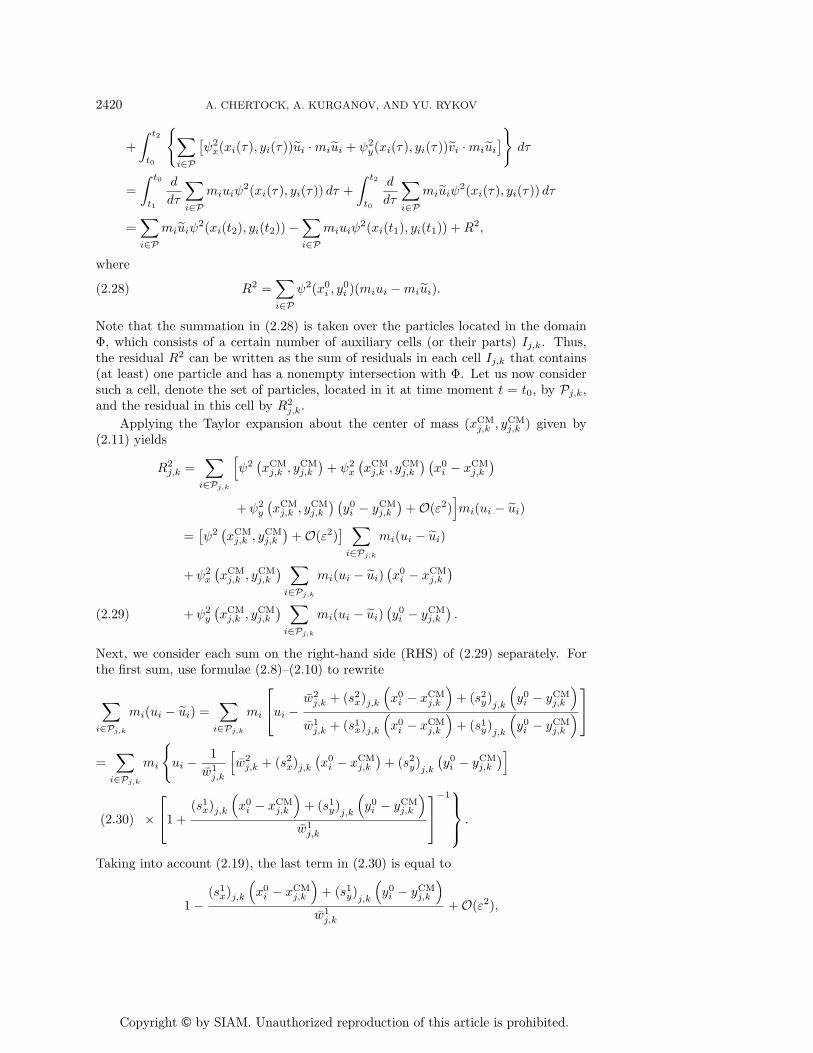
In this example, a δ-shock develops immediately and propagates with speed 0.2.We take Δx = 0.005 for the CU scheme and the initial uniform distribution
of particles, placed Δx away from each other, for the SP method. In Figure 1,the particle/cell masses and the corresponding velocities, computed by both the SPmethod and the CU scheme, are plotted at time t = 0.5. Note that because of thepoint mass concentration occurring at the δ-shock, the masses are presented in thelogarithmic scale so that a more detailed structure of the solution can be seen.
Copyright © by SIAM. Unauthorized reproduction of this article is prohibited.
2424 A. CHERTOCK, A. KURGANOV, AND YU. RYKOV
−0.5 0 0.5−7
−6
−5
−4
−3
−2
−1
ln(m
)
massSPCU
−0.5 0 0.5
−0.4
−0.2
0
0.2
0.4
0.6
u
velocitySPCU
Fig. 1. Solution of (1.2), (3.1) computed by the SP method and the CU scheme.
Figure 1 demonstrates that both schemes are able to capture the δ-shock withthe correct propagation speed, but one can clearly see the superiority of the resultsobtained by the SP method, which does not smear the δ-shock.
Example 2. We consider a test problem of the collision of two compactly sup-ported clouds. The initial data, prescribed at t = −1, are taken from [17],
(3.2) (ρ(x,−1), u(x,−1)) =
⎧⎨⎩(2, 1) if −2 < x < −1,(1,−1) if 1 < x < 5,(0, 0) otherwise.
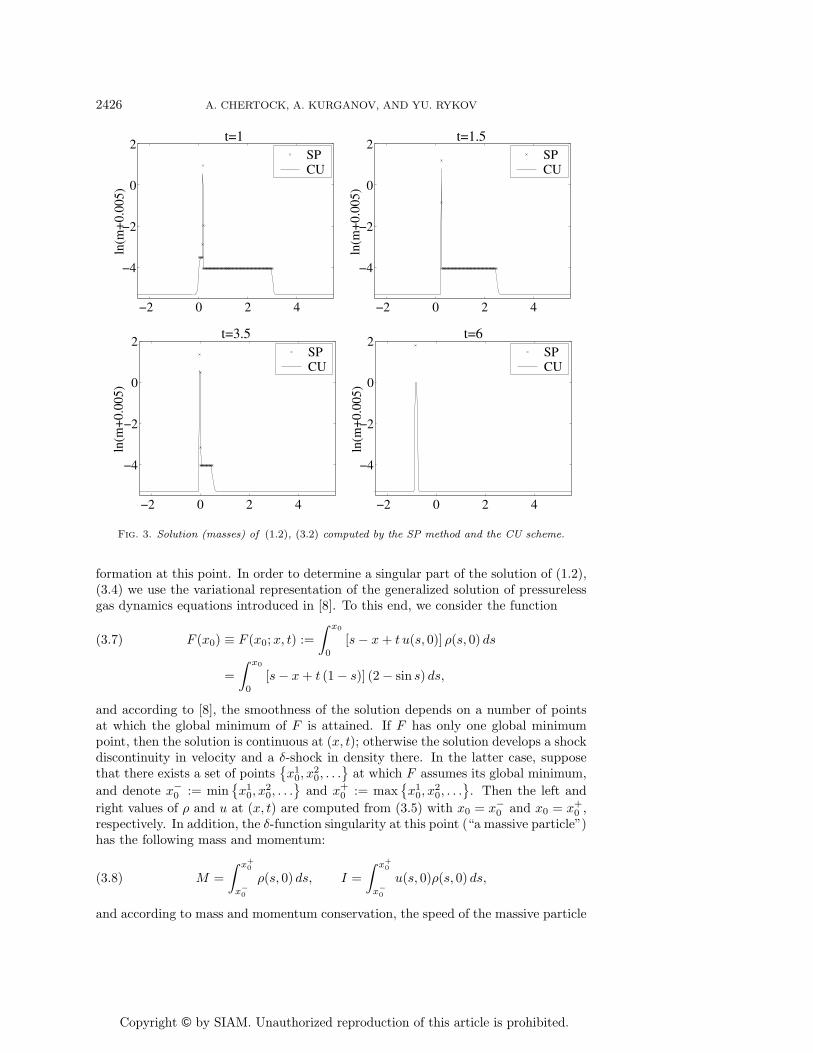
The two clouds collide at time t = 0. The left cloud is fully accelerated into the δ-waveat about t ≈ 1.21 and the right cloud is fully accelerated at about t ≈ 4.25. We use auniform spatial grid with Δx = 0.0125 for the CU scheme. The SP method is startedwith 400 particles, placed only in the intervals [−2,−1] and [1, 5], where the dust isinitially present. Figures 2 and 3 show the particle/cell masses (in the logarithmicscale) at times t = −1, −0.5, 0, 0.5, 1, 1.5, 3.5, and 6. As one can observe, bothmethods give the same correct location of the δ-wave. However, both the δ-wave andthe contact discontinuities computed by the CU scheme are smeared over a numberof cells, while the resolution achieved by the SP method is almost perfect. We notethat the mass computed by the SP method is concentrated in a single point by timet = 6.
Example 3. In this example, we demonstrate an interaction of two singularshocks by numerically solving the system (1.2) subject to the following initial data:
(3.3) (ρ(x, 0), u(x, 0)) =
⎧⎪⎪⎨⎪⎪⎩(0.25, 1.00) if −2.75 < x < −0.75,(0.25, 0.50) if −0.75 < x < 0.5,
(1.00,−1.00) if 0.5 < x < 1.5,(0.00, 0.00) otherwise.
In Figure 4, we plot the particle/cell masses (in the logarithmic scale) computed byboth the SP method and the CU scheme at times t = 0, 0.5, 1, 1.5, 2, and 2.5. We startthe SP method with N = 425 particles, which are uniformly distributed in the interval[−2.75, 1.5]. For the CU scheme, we use a uniform spatial grid with Δx = 0.01. Again,one can clearly see that the SP method outperforms the finite-volume CU scheme byfar.

Copyright © by SIAM. Unauthorized reproduction of this article is prohibited.
PARTICLE METHOD FOR PRESSURELESS GAS DYNAMICS 2425
−2 0 2 4
−4
−2
0
2
ln(m
+0.
005)
t=−1
−2 0 2 4
−4
−2
0
2
ln(m
+0.
005)
t=−0.5SPCU
−2 0 2 4
−4
−2
0
2
ln(m
+0.
005)
t=0SPCU
−2 0 2 4
−4
−2
0
2ln
(m+
0.00
5)
t=0.5SPCU
Fig. 2. Solution (masses) of (1.2), (3.2) computed by the SP method and the CU scheme.
Example 4. The last 1-D example is devoted to a problem where the velocityu changes its sign in the region with varying density. This significantly increasesthe level of complexity of the problem due to a special way the singularity forms, asdemonstrated below.
We consider the system (1.2) subject to the smooth initial data:(3.4)
ρ(x, 0) =
{2 − sinx if −π ≤ x ≤ π,
0 otherwise,u(x, 0) =
{1 − x if −π ≤ x ≤ π,
0 otherwise,
for which the exact solution can be found analytically as follows. A continuous partof the solution is obtained by the method of characteristics:
(3.5) u(X(t), t) = 1 − x0, ρ(X(t), t) =2 − sinx0
1 − t,
where
(3.6) X(t) = x0 + t(1 − x0)
is the characteristic line starting at x = x0. Obviously, the solution (3.5)–(3.6) isvalid in the domain bounded by the characteristics X−(t) = −π + t(1 + π) andX+(t) = π + t(1 − π) and thus exists until t = 1 only; see Figure 5.
As t approaches 1, the density tends to infinity, more and more mass is con-centrated near the point x = 1, and therefore one can anticipate a massive particle
Copyright © by SIAM. Unauthorized reproduction of this article is prohibited.
2426 A. CHERTOCK, A. KURGANOV, AND YU. RYKOV
−2 0 2 4
−4
−2
0
2
ln(m
+0.
005)
t=1SPCU
−2 0 2 4
−4
−2
0
2
ln(m
+0.
005)
t=1.5SPCU
−2 0 2 4
−4
−2
0
2
ln(m
+0.
005)
t=3.5SPCU
−2 0 2 4
−4
−2
0
2ln
(m+
0.00
5)
t=6SPCU
Fig. 3. Solution (masses) of (1.2), (3.2) computed by the SP method and the CU scheme.
formation at this point. In order to determine a singular part of the solution of (1.2),(3.4) we use the variational representation of the generalized solution of pressurelessgas dynamics equations introduced in [8]. To this end, we consider the function
F (x0) ≡ F (x0;x, t) :=
∫ x0
0
[s− x + t u(s, 0)] ρ(s, 0) ds(3.7)
=
∫ x0
0
[s− x + t (1 − s)] (2 − sin s) ds,
and according to [8], the smoothness of the solution depends on a number of pointsat which the global minimum of F is attained. If F has only one global minimumpoint, then the solution is continuous at (x, t); otherwise the solution develops a shockdiscontinuity in velocity and a δ-shock in density there. In the latter case, supposethat there exists a set of points
{x1
0, x20, . . .
}at which F assumes its global minimum,
and denote x−0 := min
{x1
0, x20, . . .
}and x+
0 := max{x1
0, x20, . . .
}. Then the left and
right values of ρ and u at (x, t) are computed from (3.5) with x0 = x−0 and x0 = x+
0 ,respectively. In addition, the δ-function singularity at this point (“a massive particle”)has the following mass and momentum:
(3.8) M =
∫ x+0
x−0
ρ(s, 0) ds, I =
∫ x+0
x−0
u(s, 0)ρ(s, 0) ds,
and according to mass and momentum conservation, the speed of the massive particle

Copyright © by SIAM. Unauthorized reproduction of this article is prohibited.
PARTICLE METHOD FOR PRESSURELESS GAS DYNAMICS 2427
−3 −2 −1 0 1
−5
−4
−3
−2
−1
0
1 t=0
ln(m
+0.
005)
−3 −2 −1 0 1
−5
−4
−3
−2
−1
0
1
ln(m
+0.
005)
t=0.5SPCU
−3 −2 −1 0 1
−5
−4
−3
−2
−1
0
1
ln(m
+0.
005)
t=1SPCU
−3 −2 −1 0 1
−5
−4
−3
−2
−1
0
1ln
(m+
0.00
5)
t=1.5SPCU
−3 −2 −1 0 1
−5
−4
−3
−2
−1
0
1
ln(m
+0.
005)
t=2SPCU
−3 −2 −1 0 1
−5
−4
−3
−2
−1
0
1
ln(m
+0.
005)
t=2.5SPCU
Fig. 4. Solution (masses) of (1.2), (3.3) computed by the SP method and the CU scheme.
is
(3.9)dX
dt=
I
M.
For the problem under consideration, the singularity is first formed at the point(x, t) = (1, 1), and for t ≥ 1, the global minimum of F is attained at two pointsonly: x−
0 = −π and x+0 = π. Therefore, by t = 1 all the mass is concentrated in
one massive particle with the mass M = 4π and the momentum I = 6π (accordingto (3.8)), and the movement of this particle is described, according to (3.9), by theformula X(t) = (3t− 1)/2, t ≥ 1; see Figure 5.

Copyright © by SIAM. Unauthorized reproduction of this article is prohibited.
2428 A. CHERTOCK, A. KURGANOV, AND YU. RYKOV
1
1
x=X- (t) x=X+ (t)
x=X(t)
x
t
−π π
Fig. 5. Characteristics diagram for the initial-value problem (1.2), (3.4).
−2 0 2
0.02
0.03
0.04
0.05mass
t=0t=0.5t=0.97
1 1.5 2 2.50
2
4
6
8
10
12
14mass
t=1t=1.02t=1.03t=1.5t=2
Fig. 6. Solution (masses) of (1.2), (3.4) computed by the SP method for t < 1 (left), when thesolution is smooth inside its shrinking support, and for t ≥ 1 (right), when the total mass M = 4πis concentrated in one particle, propagating with the constant speed I/M = 3/2. Note that due toa certain arbitrariness in the selection of the unification parameter dcr, the final collapse of thenumerical solution occurs at a slightly later time t ≈ 1.03.
We now turn to the presentation of our numerical results. We start the SPsimulations with 400 particles uniformly distributed over the interval [−π, π]. InFigure 6, we plot the particle masses computed by the SP method only, since the CUscheme could not be applied to this problem at large times (t ∼ 1 and larger). Wenote that, as indicated in [17], other finite-volume methods are likely to fail to capturethe solution of the initial-value problem (1.2), (3.4) as well.
3.2. Two-dimensional examples.
Example 5. We start by numerically solving the 2-D analogue of the 1-D problemconsidered in Example 1, namely, we solve the system (1.5) in the square domain[−1, 1] × [−1, 1] subject to the 1-D Riemann initial data, artificially extended to twospace dimensions:
(3.10) (ρ(x, y, 0), u(x, y, 0), v(x, y, 0)) =
{(1.00, 0.5, 0) if x < 0,(0.25,−0.4, 0) if x > 0.
The purpose of this simple example is to demonstrate the failure of the “standard”velocity recovery procedure (2.7) and the ability of the alternative procedure (2.9),developed in section 2.1, to force the desired interaction of nearby particles.

Copyright © by SIAM. Unauthorized reproduction of this article is prohibited.
PARTICLE METHOD FOR PRESSURELESS GAS DYNAMICS 2429
Recall that in this example a δ-shock develops immediately at the line x = 0and then propagates to the right with speed 0.2. As has been already mentioned,the probability of collision of two particles approaching the same singularity curve intwo dimensions is, in general, zero, and therefore using formula (2.7) for computingvelocities requires a special symmetric setting of the initial locations of particles; seeFigure 7 (left). Obviously, if at time t = 0 the particles are placed as shown in Figure 7(right) and if the unification parameter is reasonably small (dcr < Δy/2), the particlesmoving from the left and from the right will never interact and the δ-shock will notbe captured numerically. We note that for a more complicated, truly 2-D initial datait may be impossible to impose any kind of symmetry, so the situation with the dataas in Figure 7 (right) is generic.
Fig. 7. Initial locations of particles in Example 5: symmetric (left) and asymmetric (right) cases.
On the other hand, the velocity recovery procedure (2.9) ensures an interactionbetween particles independently of their initial placement. In Figures 8 and 9, weshow the masses and x-velocities of the particles at time t = 0.5. They are computedby the SP method with the initial locations of particles as in Figure 7 (left) and Figure7 (right), respectively. As one can see, in both cases the SP method combined withthe velocity recovery procedure (2.9) leads to the desired clustering of particles atthe singularity. Moreover, the resolution achieved in the case of asymmetric initialparticle distribution is almost as good as in the symmetric case.
Example 6. Next, we turn to genuinely 2-D problems. First, consider the system(1.5) subject to the following initial data:
(3.11) (ρ(x, y, 0), u(x, y, 0), v(x, y, 0)) =
⎧⎨⎩(2, 2, 1) if (x, y) ∈ Ω,(0, 0, 0) if (x, y) ∈ ∂Ω,(1, 0, 0) otherwise,
where Ω = {x < 0, y < 1} ∪{x > 0, y > 0, x2 + y2 < 1
}∪ {y < 0, 0 < x < 1}. The
initial location of the discontinuity ∂Ω is shown in Figure 10. According to [21], theexact solution of the initial-value problem (1.5), (3.11) develops a δ-shock in density,

Copyright © by SIAM. Unauthorized reproduction of this article is prohibited.
2430 A. CHERTOCK, A. KURGANOV, AND YU. RYKOV
−0.5 0 0.5−7
−6
−5
−4
−3
−2
−1mass
ln(m
)
−0.5 0 0.5
−0.4
−0.2
0
0.2
0.4
0.6 x−velocity
u
Fig. 8. Side view on the solution of (1.5), (3.10) computed by the SP method. The initiallocation of particles is shown in Figure 7 (left).
−0.5 0 0.5−7
−6
−5
−4
−3
−2
−1mass
ln(m
)
−0.5 0 0.5
−0.4
−0.2
0
0.2
0.4
0.6 x−velocity
u
Fig. 9. Side view on the solution of (1.5), (3.10) computed by the SP method. The initiallocation of particles is shown in Figure 7 (right).
and the evolution of the shock curve is described by the following system of ODEs:
(3.12)
⎧⎪⎪⎪⎪⎨⎪⎪⎪⎪⎩dX
dt= u−
√ρ−√
ρ− +√ρ+
=2√
2√2 + 1
,
dY
dt= v−
√ρ−√
ρ− +√ρ+
=
√2√
2 + 1,
where (ρ−, u−, v−) := (2, 2, 1) are the initial values inside the domain Ω and ρ+ := 1is the initial value of the density on the other side of the initial shock curve.
Numerically, we restrict the initial data (3.11) to the finite domain [−4, 4]×[−4, 4]and consider the following initial-boundary value problem: (1.5), (3.11) together withthe solid wall boundary conditions. The numerical solutions, computed by the SPmethod at time t = 2 with 50 × 50 and 100 × 100 initially uniformly distributedparticles, are plotted in Figure 10. The size of each point in the figure is proportionalto the mass accumulated in the particle located there. The exact solution of theinitial-boundary value problem is not known, but in the domain [0, 4] × [−2, 4] itcoincides with the solution of the original initial-value problem (1.5), (3.11), and ascan be clearly seen in Figure 10, the SP method accurately tracks the evolution of

Copyright © by SIAM. Unauthorized reproduction of this article is prohibited.
PARTICLE METHOD FOR PRESSURELESS GAS DYNAMICS 2431
−4 −2 0 2 4−4
−2
0
2
4
initial shock location
−4 −2 0 2 4−4
−2
0
2
4
initial shock location
Fig. 10. Top view on the solution (masses) of (1.5), (3.11) computed by the SP method with50× 50 (left) and 100× 100 (right) particles. The solid line is obtained from the initial shock curve(the dashed line) by the evolution according to (3.12).
the corresponding part of the shock curve described by (3.12). Outside the domain[0, 4] × [−2, 4], the solution is obviously affected by the boundedness of the cloud,but the obtained numerical solution looks reasonable, as supported by the performedmesh refinement study.
Example 7. Next, we consider an example with nonzero mass and momenta atthe initial shock curve. We numerically solve the system (1.5) subject to the followinginitial data:
(3.13) (ρ(x, 0), u(x, 0), v(x, 0)) =
⎧⎨⎩(2, 2, 2) if x ∈ Ω,
(10 δ(dist(x, ∂Ω)), 2, 1) if x ∈ ∂Ω,(2, 0, 0) otherwise,
where x ≡ (x, y) and the domain Ω is the same as in Example 6: Ω = {x < 0, y < 1}∪{x > 0, y > 0, x2 +y2 < 1
}∪{y < 0, 0 < x < 1}. In the practical implementation, we
replace the δ-function along the curve ∂Ω with its approximation by a step function;namely, we take
ρ(x, 0) =
⎧⎪⎪⎨⎪⎪⎩10√
2√(Δx)
2+ (Δy)
2if dist(x, ∂Ω) ≤
√(Δx)
2+ (Δy)
2
2√
2,
2 otherwise.
The numerical solutions at time t = 1.5 obtained using the SP method with101 × 101 particles (initially uniformly distributed) and the CU scheme with Δx =Δy = 0.08 are plotted in Figures 11 and 12. Note that the maximal mass value of thesolution obtained by the CU scheme is 0.6299 while the maximal mass obtained by theSP method is 2.7009. As before, the size of each point in the figures is proportionalto the mass accumulated in the particle located there.
Even though a complete structure of the exact solution of the initial-value problem(1.5), (3.13) is not available, the obtained solution behavior has been expected (seethe discussion at the end of section 2). It is instructive to compare the computednumerical solution with theoretical results presented in [21]. According to [21], if

Copyright © by SIAM. Unauthorized reproduction of this article is prohibited.
2432 A. CHERTOCK, A. KURGANOV, AND YU. RYKOV
−4−2
02
4 −4−2
02
4
0.5
1
1.5
2
2.5
−4−2
02
4 −4−2
02
4
0.2
0.4
0.6
Fig. 11. Solution (masses) of (1.5), (3.13) computed by the SP method (left) and the CUscheme (right).
−4 −2 0 2 4−4
−2
0
2
4
initial shock location
−4 −2 0 2 4−4
−2
0
2
4
initial shock location
Fig. 12. Top view on the solution (masses) of (1.5), (3.13) computed by the SP method (left)and the CU scheme (right). The solid lines are obtained from the initial shock curve (the dashedline) by the evolution according to (3.14).
initially a shock curve with mass distribution P0 and velocities (U0, V0) is locatedalong the line x0(l) = C ≡ const, y0(l) = l, then its location at a later time is givenby
(3.14)
⎧⎪⎪⎪⎪⎪⎨⎪⎪⎪⎪⎪⎩x = C +
[u
2−(
12u− U0
)P0
ρut + P0
]t,
uy − vx =(uV0 − vU0)P0
ρuln
(1 +
ρut
P0
)+ ul − vC,
where ρ, u, and v are the density and the corresponding velocities inside the domain.If we now consider a part of the initial shock curve ∂Ω, namely, x0 = 1, y0 = l,0 ≤ l ≤ 1, and substitute the corresponding values of P0 = 10, U0 = 2, V0 = 1, andρ = u = v = 2 into the first formula in (3.14), we obtain that at time t = 1.5 the shockline should be located at x = 3.4375. Similarly, it can be shown that the initial shockline x0 = l, y0 = 1, 0 ≤ l ≤ 1 should move to y = 2.5 by the time t = 1.5. As one cansee from Figure 12, both methods accurately track the evolution of the corresponding
Copyright © by SIAM. Unauthorized reproduction of this article is prohibited.
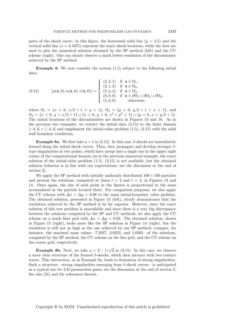
PARTICLE METHOD FOR PRESSURELESS GAS DYNAMICS 2433
parts of the shock curve: in this figure, the horizontal solid line (y = 2.5) and thevertical solid line (x = 3.4375) represent the exact shock locations, while the dots areused to plot the numerical solution obtained by the SP method (left) and the CUscheme (right). One can clearly observe a much better resolution of the discontinuityachieved by the SP method.
Example 8. We now consider the system (1.5) subject to the following initialdata:
(3.15) (ρ(x, 0), u(x, 0), v(x, 0)) =
⎧⎪⎪⎪⎪⎨⎪⎪⎪⎪⎩(2, 2, 1) if x ∈ Ω1,(2, 1, 2) if x ∈ Ω2,(2, η, η) if x ∈ Ω3,(0, 0, 0) if x ∈ ∂Ω1 ∪ ∂Ω2 ∪ ∂Ω3,(1, 0, 0) otherwise,
where Ω1 = {x < 0, x/2 + 1 < y < 1}, Ω2 = {y < 0, y/2 + 1 < x < 1}, andΩ3 = {x < 0, y < x/2 + 1} ∪ {x > 0, y > 0, x2 + y2 < 1} ∪ {y < 0, x < y/2 + 1}.The initial locations of the discontinuities are shown in Figures 13 and 16. As inthe previous two examples, we restrict the initial data (3.15) to the finite domain[−4, 4] × [−4, 4] and supplement the initial-value problem (1.5), (3.15) with the solidwall boundary conditions.
Example 8a. We first take η = 1 in (3.15). In this case, δ-shocks are immediatelyformed along the initial shock curves. Then, they propagate and develop stronger δ-type singularities at two points, which later merge into a single one in the upper rightcorner of the computational domain (as in the previous numerical example, the exactsolution of the initial-value problem (1.5), (3.15) is not available, but the obtainedsolution behavior is in line with our expectations; see the discussion at the end ofsection 2).
We apply the SP method with initially uniformly distributed 100× 100 particlesand present the solutions, computed at times t = 2 and t = 4, in Figures 13 and14. Once again, the size of each point in the figures is proportional to the massaccumulated in the particle located there. For comparison purposes, we also applythe CU scheme with Δx = Δy = 0.08 to the same initial-boundary value problem.The obtained solution, presented in Figure 15 (left), clearly demonstrates that theresolution achieved by the SP method is by far superior. However, since the exactsolution of this test problem is unavailable and since there is a very big discrepancybetween the solutions computed by the SP and CU methods, we also apply the CUscheme on a much finer grid with Δx = Δy = 0.02. The obtained solution, shownin Figure 15 (right), looks more like the SP solution in Figure 14 (right), but theresolution is still not as high as the one achieved by our SP method; compare, forinstance, the maximal mass values—7.2927, 3.9223, and 1.0205—of the solutions,computed by the SP method, the CU scheme on the fine grid, and the CU scheme onthe coarse grid, respectively.
Example 8b. Next, we take η = 2 − 1/√
2 in (3.15). In this case, we observea more clear structure of the formed δ-shocks, which then interact with two contactwaves. This interaction, as in Example 8a, leads to formation of strong singularities.Such a structure—strong singularities emerging from δ-shock curves—is anticipatedas a typical one for 2-D pressureless gases; see the discussion at the end of section 2.See also [21] and the references therein.

Copyright © by SIAM. Unauthorized reproduction of this article is prohibited.
2434 A. CHERTOCK, A. KURGANOV, AND YU. RYKOV
−4 −2 0 2 4−4
−2
0
2
4t=2
Ω1
Ω3 Ω
2
−4 −2 0 2 4−4
−2
0
2
4t=4
Ω3
Ω2
Ω1
Fig. 13. Top view on the solution (masses) of (1.5), (3.15) with η = 1 at t = 2 (left) and t = 4(right) computed by the SP method. The dashed lines represent the initial location of discontinuities.
−4−2
02
4 −4−2
02
4
0.2
0.4
0.6
0.8
t=2
−4−2
02
4 −4−2
02
4
2
4
6
t=4
Fig. 14. Solution (masses) of (1.5), (3.15) with η = 1 at t = 2 (left) and t = 4 (right) computedby the SP method.
−4−2
02
4 −4−2
02
4
0.2
0.4
0.6
0.8
1
t=4
−4−2
02
4 −4−2
02
4
1
2
3
t=4
Fig. 15. Solution (masses) of (1.5), (3.15) with η = 1 at t = 4 computed by the CU schemewith Δx = Δy = 0.08 (left) and Δx = Δy = 0.02 (right).
Copyright © by SIAM. Unauthorized reproduction of this article is prohibited.
PARTICLE METHOD FOR PRESSURELESS GAS DYNAMICS 2435
−4 −2 0 2 4−4
−2
0
2
4t=1.7
Ω1
Ω3
Ω2
−4 −2 0 2 4−4
−2
0
2
4t=3
Ω1
Ω3
Ω2
Fig. 16. Top view on the solution (masses) of (1.5), (3.15) with η = 2− 1/√
2 at t = 1.7 (left)and t = 3 (right) computed by the SP method. The dashed lines represent the initial shock location.
−4−2
02
4 −4−2
02
4
0.2
0.4
0.6
0.8
t=1.7
−4−2
02
4 −4−2
02
4
0.51
1.52
2.5
t=3
Fig. 17. Solution (masses) of (1.5), (3.15) with η = 2−1/√
2 at t = 1.7 (left) and t = 3 (right)computed by the SP method.
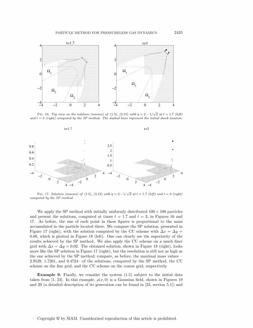
We apply the SP method with initially uniformly distributed 100× 100 particlesand present the solutions, computed at times t = 1.7 and t = 3, in Figures 16 and17. As before, the size of each point in these figures is proportional to the massaccumulated in the particle located there. We compare the SP solution, presented inFigure 17 (right), with the solution computed by the CU scheme with Δx = Δy =0.08, which is plotted in Figure 18 (left). One can clearly see the superiority of theresults achieved by the SP method. We also apply the CU scheme on a much finergrid with Δx = Δy = 0.02. The obtained solution, shown in Figure 18 (right), looksmore like the SP solution in Figure 17 (right), but the resolution is still not as high asthe one achieved by the SP method; compare, as before, the maximal mass values—2.9529, 1.7261, and 0.4724—of the solutions, computed by the SP method, the CUscheme on the fine grid, and the CU scheme on the coarse grid, respectively.
Example 9. Finally, we consider the system (1.5) subject to the initial datataken from [1, 23]. In this example, ρ(x, 0) is a Gaussian field, shown in Figures 19and 20 (a detailed description of its generation can be found in [23, section 5.1]) and

Copyright © by SIAM. Unauthorized reproduction of this article is prohibited.
2436 A. CHERTOCK, A. KURGANOV, AND YU. RYKOV
−4−2
02
4 −4−2
02
4
0.1
0.2
0.3
0.4
t=3
−4−2
02
4 −4−2
02
4
0.5
1
1.5
t=3
Fig. 18. Solution (masses) of (1.5), (3.15) with η = 2 − 1/√
2 at t = 3 computed by the CUscheme with Δx = Δy = 0.08 (left) and Δx = Δy = 0.02 (right).
the initial velocity vector is the solution of the following elliptic problem:
(3.16)
⎧⎨⎩u = −φx,v = −φy,Δφ = 4πG(ρ− ρ) in Ω = [0, 251] × [0, 251],
where G is the gravitational constant and ρ = 1|Ω|
∫Ωρ dx dy. All the boundary condi-
tions are assumed to be periodic. These 2-D physical data are derived from large-scalestructure simulations related to the cosmological model of Zeldovich [24]. In Figures19 and 20, we observe the formation of the large-scale structures computed by theSP method and the CU scheme, respectively. We use a uniform spatial grid withΔx = Δy = 1 for the CU scheme and the uniform initial distribution of 251 × 251particles. In order to compare the results, the total mass of each cell computed by theCU scheme has been recalculated at the location of particles. Again, the size of eachpoint in Figures 19 and 20 is proportional to the total mass at this point, that is, big-ger points correspond to larger masses. As one can see, for small times both schemesproduce very similar results, while for larger times a numerical diffusion present inthe CU scheme “takes over” (compare the corresponding results at times t = 4000and t = 15000 in Figures 19 and 20). In fact, the maximum mass accumulated at onepoint by the SP method is about 15 times larger than the one accumulated by the CUscheme. We also would like to point out that, as a result of unification of clusteringparticles, the number of particles is decreasing in time and therefore the efficiency ofthe SP method is increasing. For instance, the number of particles at times t = 1000,4000, and 15000 is 2767, 1068, and 454, respectively, while computations using theCU scheme are being performed on a 251× 251 grid for all times. This also results inmuch smaller runtime for the SP method compared to the CU scheme.
4. Concluding remarks. We have presented a new sticky particle (SP) methodfor the system of Euler equations of pressureless gas dynamics that arises in the mod-eling of the formation of large-scale structures in the universe. The main feature ofinterest in this problem is the formation of strong singularities (δ-functions along thesurfaces as well as at separate points) and the emergence of vacuum states, and there-fore particle methods seem to be a natural choice for numerical simulations of suchmodels. The proposed SP method has been studied both analytically and numerically.

Copyright © by SIAM. Unauthorized reproduction of this article is prohibited.
PARTICLE METHOD FOR PRESSURELESS GAS DYNAMICS 2437
Fig. 19. Top view on the solution (masses) of (1.5), (3.16) computed by the SP method atdifferent times.
It has been shown that the particle approximation satisfies the original system of pres-sureless gas dynamics in a weak sense, but only within a certain residual, which hasbeen rigorously estimated. It has also been explained why the relevant errors shoulddiminish as the total number of particles increases. Numerical experiments in oneand two space dimensions have been performed (3-D extension of the SP method isout of scope of this paper, but it can be carried out rather straightforwardly). TheSP method has been compared to the second-order CU scheme. Our numerical ex-periments clearly demonstrate the superiority of results obtained by the SP method,which seems to be a robust, accurate, and efficient alternative to existing numericalmethods for pressureless gas dynamics.
Appendix A. Semidiscrete central-upwind schemes for pressureless gasdynamics. Here, we briefly describe semidiscrete CU schemes for the 2-D systemof pressureless gas dynamics (1.5), which can be written in the following flux-vectorform:
wt + f(w)x + g(w)y = 0,

Copyright © by SIAM. Unauthorized reproduction of this article is prohibited.
2438 A. CHERTOCK, A. KURGANOV, AND YU. RYKOV
Fig. 20. Top view on the solution (masses) of (1.5), (3.16) computed by the CU scheme atdifferent times.
where
w :=
⎛⎝ ρρuρv
⎞⎠ , f(w) :=
⎛⎝ ρuρu2
ρuv
⎞⎠ , g(w) :=
⎛⎝ ρvρuvρv2
⎞⎠ .
We consider a uniform spatial grid xμ := μΔx, yν := νΔy, and denote thecomputed quantities, the cell averages, by
wj,k(t) :=1
ΔxΔy
∫∫Ij,k
w(ξ, η, t) dη dξ, Ij,k := [xj− 12, xj+ 1
2] × [yk− 1
2, yk+ 1
2].
The cell averages are evolved in time according to the semidiscrete CU scheme
d
dtwj,k(t) = −
Hxj+ 1
2 ,k(t) −Hx
j− 12 ,k
(t)
Δx−
Hy
j,k+ 12
(t) −Hy
j,k− 12
(t)
Δy,

Copyright © by SIAM. Unauthorized reproduction of this article is prohibited.
PARTICLE METHOD FOR PRESSURELESS GAS DYNAMICS 2439
where the numerical fluxes Hxj+ 1
2 ,kand Hy
j,k+ 12
are given by (see [11] for the derivation)
(A.1)
Hxj+ 1
2 ,k=
a+j+ 1
2 ,kf(wE
j,k) − a−j+ 1
2 ,kf(wW
j+1,k)
a+j+ 1
2 ,k− a−
j+ 12 ,k
+a+j+ 1
2 ,ka−j+ 1
2 ,k
[wW
j+1,k − wEj,k
a+j+ 1
2 ,k− a−
j+ 12 ,k
− qxj+ 1
2 ,k
]
and(A.2)
Hy
j,k+ 12
=b+j,k+ 1
2
g(wNj,k) − b−
j,k+ 12
g(wSj,k+1)
b+j,k+ 1
2
− b−j,k+ 1
2
+b+j,k+ 1
2
b−j,k+ 1
2
[wS
j,k+1 − wNj,k
b+j,k+ 1
2
− b−j,k+ 1
2
− qy
j,k+ 12
].
Note that all the quantities in (A.1) and (A.2) depend on t, but we will omit thisdependence in order to simplify the notation.
In (A.1)–(A.2), the point values wE(W,S,N) are to be computed from a conserva-tive, nonoscillatory piecewise polynomial reconstruction of an appropriate order. Forexample, the second-order CU scheme would employ a piecewise linear reconstruction
(A.3) w(x, y, t) = wj,k(t) + (wx)j,k(x− xj) + (wy)j,k(y − yk) for (x, y) ∈ Ij,k,
and the corresponding point values will be
wE(W)j,k := wj,k(t) ±
Δx
2(wx)j,k, w
N(S)j,k := wj,k(t) ±
Δy
2(wy)j,k.
To ensure a nonoscillatory property of this reconstruction and thus of the second-order CU scheme, the slopes in (A.3) should be computed with the help of a nonlinearlimiter. In our numerical experiments, we have used a one-parameter family of theminmod limiters [15, 18, 22]:
(wx)j,k = minmod
(θwj+1,k − wj,k
Δx,wj+1,k − wj−1,k
2Δx, θ
wj,k − wj−1,k
Δx
),
(wy)j,k = minmod
(θwj,k+1 − wj,k
Δy,wj,k+1 − wj,k−1
2Δy, θ
wj,k − wj,k−1
Δy
),
where θ ∈ [1, 2], and the multivariate minmod function is defined by (2.14). Noticethat larger θ’s correspond to less dissipative but, in general, more oscillatory limiters(we have used θ = 1.5 in all the reported numerical experiments).
Since all the eigenvalues of the Jacobians ∂f∂w and ∂g
∂w are of multiplicity 3 andare equal to u and v, respectively, the one-sided local speeds in (A.1)–(A.2) are easyto estimate:
a+j+ 1
2 ,k:= max
{uWj+1,k, u
Ej,k, 0
}, a−
j+ 12 ,k
:= min{uWj+1,k, u
Ej,k, 0
},
b+j,k+ 1
2
:= max{vSj,k+1, v
Nj,k, 0
}, b−
j,k+ 12
:= min{vSj,k+1, v
Nj,k, 0
}.
Finally, qxj+ 1
2 ,kand qy
j,k+ 12
are the “antidiffusion” terms that help to reduce numerical
dissipation present at nonoscillatory central schemes [11]:
qxj+ 1
2 ,k= minmod
(wNW
j+1,k − wintj+ 1
2 ,k
a+j+ 1
2 ,k− a−
j+ 12 ,k
,wint
j+ 12 ,k
− wNEj,k
a+j+ 1
2 ,k− a−
j+ 12 ,k
,
wSWj+1,k − wint
j+ 12 ,k
a+j+ 1
2 ,k− a−
j+ 12 ,k
,wint
j+ 12 ,k
− wSEj,k
a+j+ 1
2 ,k− a−
j+ 12 ,k
),

Copyright © by SIAM. Unauthorized reproduction of this article is prohibited.
2440 A. CHERTOCK, A. KURGANOV, AND YU. RYKOV
qy
j,k+ 12
= minmod
(wSW
j,k+1 − wintj,k+ 1
2
b+j,k+ 1
2
− b−j,k+ 1
2
,wint
j,k+ 12
− wNWj,k
b+j,k+ 1
2
− b−j,k+ 1
2
,
wSEj,k+1 − wint
j,k+ 12
b+j,k+ 1
2
− b−j,k+ 1
2
,wint
j,k+ 12
− wNEj,k
b+j,k+ 1
2
− b−j,k+ 1
2
),
where
wintj+ 1
2 ,k=
a+j+ 1
2 ,kwW
j+1,k − a−j+ 1
2 ,kwE
j,k −{f(wW
j+1,k) − f(wEj,k)
}a+j+ 1
2 ,k− a−
j+ 12 ,k
,
wintj,k+ 1
2=
b+j,k+ 1
2
wSj,k+1 − b−
j,k+ 12
wNj,k −
{g(wS
j,k+1) − g(wNj,k)
}b+j,k+ 1
2
− b−j,k+ 1
2
,
and the point values at the cell corners are
wNE(NW)j,k := wj,k(t) ±
Δx
2(wx)j,k +
Δy
2(wy)j,k,
wSE(SW)j,k := wj,k(t) ±
Δx
2(wx)j,k − Δy
2(wy)j,k.
REFERENCES
[1] C. Berthon, M. Breuss, and M.-O. Titeux, A relaxation scheme for the approximation of thepressureless Euler equations, Numer. Methods Partial Differential Equations, 22 (2006),pp. 484–505.
[2] F. Bouchut, On zero pressure gas dynamics, in Advances in Kinetic Theory and Computing,World Scientific, River Edge, NJ, 1994, pp. 171–190.
[3] F. Bouchut and G. Bonnaud, Numerical simulation of relativistic plasmas in hydrodynamicregime, Z. Angew. Math. Mech., 76 (1996), pp. 287–290.
[4] F. Bouchut and F. James, Duality solutions for pressureless gases, monotone scalar conserva-tion laws, and uniqueness, Comm. Partial Differential Equations, 24 (1999), pp. 2173–2189.
[5] F. Bouchut, S. Jin, and X. Li, Numerical approximations of pressureless and isothermal gasdynamics, SIAM J. Numer. Anal., 41 (2003), pp. 135–158.
[6] Y. Brenier and E. Grenier, Sticky particles and scalar conservation laws, SIAM J. Numer.Anal., 35 (1998), pp. 2317–2328.
[7] G.-Q. Chen and H. Liu, Formation of δ-shocks and vacuum states in the vanishing pressurelimit of solutions to the Euler equations for isentropic fluids, SIAM J. Math. Anal., 34(2003), pp. 925–938.
[8] W. E, Yu. G. Rykov, and Ya. G. Sinai, Generalized variational principles, global weak so-lutions and behavior with random initial data for systems of conservation laws arising inadhesion particle dynamics, Comm. Math. Phys., 177 (1996), pp. 349–380.
[9] K. O. Friedrichs, Symmetric hyperbolic linear differential equations, Comm. Pure Appl.Math., 7 (1954), pp. 345–392.
[10] S. Gottlieb, C.-W. Shu, and E. Tadmor, High order time discretization methods with thestrong stability property, SIAM Rev., 43 (2001), pp. 89–112.
[11] A. Kurganov and C.-T. Lin, On the reduction of numerical dissipation in central-upwindschemes, Commun. Comput. Phys., 2 (2007), pp. 141–163.
[12] A. Kurganov, S. Noelle, and G. Petrova, Semidiscrete central-upwind schemes for hyper-bolic conservation laws and Hamilton–Jacobi equations, SIAM J. Sci. Comput., 21 (2001),pp. 707–740.
[13] A. Kurganov and G. Petrova, Central schemes and contact discontinuities, M2AN Math.Model. Numer. Anal., 34 (2000), pp. 1259–1275.
[14] A. Kurganov and E. Tadmor, New high-resolution central schemes for nonlinear conservationlaws and convection-diffusion equations, J. Comput. Phys., 160 (2000), pp. 241–282.
[15] B. van Leer, Towards the ultimate conservative difference scheme, V. A second order sequelto Godunov’s method, J. Comput. Phys., 32 (1979), pp. 101–136.

Copyright © by SIAM. Unauthorized reproduction of this article is prohibited.
PARTICLE METHOD FOR PRESSURELESS GAS DYNAMICS 2441
[16] P. D. Lax, Weak solutions of nonlinear hyperbolic equations and their numerical computation,Comm. Pure Appl. Math., 7 (1954), pp. 159–193.
[17] R. J. LeVeque, The dynamics of pressureless dust clouds and delta waves, J. Hyperbolic Differ.Equ., 1 (2004), pp. 315–327.
[18] H. Nessyahu and E. Tadmor, Non-oscillatory central differencing for hyperbolic conservationlaws, J. Comput. Phys., 87 (1990), pp. 408–463.
[19] Yu. G. Rykov, The Numerical Method for Solving the 2-D System of Gas Dynamics withoutPressure, KIAM Preprint 76, Moscow, 1996.
[20] Yu. G. Rykov, Propagation of singularities of shock wave type in a system of equations of two-dimensional pressureless gas dynamics, Mat. Zametki, 66 (1999), pp. 760–769 (in Russian);translation in Math. Notes, 66 (1999), pp. 628–635 (2000).
[21] Yu. G. Rykov, On the nonhamiltonian character of shocks in 2-D pressureless gas, Boll.Unione Mat. Ital. Sez. B Artic. Ric. Mat. (8), 5 (2002), pp. 55–78.
[22] P. K. Sweby, High resolution schemes using flux limiters for hyperbolic conservation laws,SIAM J. Numer. Anal., 21 (1984), pp. 995–1011.
[23] M. Vergassola, B. Dubrulle, U. Frish, and A. Noullez, Burgers equations, Dervil’s stair-cases and the mass distribution for large scale structures, Astron. Astophys., 289 (1994),pp. 325–356.
[24] Ya. B. Zeldovich, Gravitational instability: An approximate theory for large density pertur-bations, Astron. Astrophys., 5 (1970), pp. 84–89.