A New Response Model for Multiple-Choice Items Randall D ...

The Distractor Model 1

A New Response Model for Multiple-Choice Items

Randall D. Penfield

University of Miami

&

Jimmy de la Torre

Rutgers, The State University of New Jersey

Paper presented at the 2008 annual meeting of the National Council on Measurement in

Education, New York.

Address for correspondence:

Randall Penfield University of Miami P.O. Box 248065 Coral Gables, FL 33124-2040 Tel: 305-284-8340 Fax: 305-284-3003 e-mail: [email protected]


Abstract

Approaches for modeling responses to multiple-choice items fall into two broad

categories: (a) those that group all distractor options into a single incorrect response

category and model the probability of correct response using a dichotomous response

model, and (b) those that retain the distinction between all response options and model

the probability of each response option using a polytomous response model. A recently

developed polytomous model for multiple-choice items is Revuelta’s (2005) generalized

distractor rejection model (DLT). A drawback of the DLT is that it is parameterized using

a form that is inconsistent with many widely used response models in educational

measurement. In this paper we propose an adaptation of the DLT called the distractor

model (DM). The DM uses a parameterization that is consistent with that of other widely

used response models in educational measurement, and thus may be more accessible and

intuitive for applied test developers than the original form of the DLT. We present the

derivation of the DM, its relationship to the parameterization of the DLT, and describe

the relationship of the DM to other polytomous response models for multiple-choice

items. In addition, we illustrate the use of the DM by applying it to responses to an

algebra test composed of multiple-choice items.

Index terms: item response theory, polytomous models, multiple-choice items


A New Response Model for Multiple-Choice Items

Multiple-choice items are a widely used item format in tests of achievement,

knowledge, and ability (Osterlind, 1998). The multiple-choice item format has the

defining property of having one option (i.e., the key) designated as the correct response,

and all other options designated as distractors or incorrect responses. Numerous response

models for multiple-choice item formats have been proposed, and these models can be

grouped into two broad categories: dichotomous and polytomous. Dichotomous models

treat the item response as a binary variable by collapsing all distractors into a single

category of incorrect response, and specifying the probability of correct response as a

function of the latent trait. Dichotomous response models include, but are not limited to,

the Rasch model (Rasch, 1960) and the one-, two-, and three-parameter logistic models

(Birnbaum, 1968; Lord, 1980). In contrast to dichotomous models, polytomous response

models retain the distinction between all response options, and specify the probability of

each possible response option as a function of the latent trait.

The advantage of using a polytomous model for multiple-choice items stems from

the potential of extracting information from the distractors as well as the correct response.

The incorporation of information pertaining to each of the distractors maximizes the

information concerning the latent trait, and thus has the potential to lead to more precise

estimation of the latent trait than the dichotomous response models, particularly at the

lower end of the latent trait continuum (Bock, 1972; De Ayala, 1989, 1992; Thissen,

1976). Polytomous models, however, contain a higher number of parameters than their

dichotomous counterparts, and thus require greater sample sizes to be effectively

implemented (De Ayala & Sava-Bolesta, 1999; DeMars, 2003).


Several polytomous response models for multiple-choice items have been

proposed. The most widely used of these models is the nominal response model (NRM;

Bock, 1972). To describe the NRM, let us consider a multiple-choice item with m

outcomes, of which m – 1 are distractor options. Let the response options be denoted by

k, where k = 1, …, m. Let us denote the response variable for the jth item by Yj, such that

a response equal to the kth option is denoted by the outcome Yj = k. Based on this

formulization, the NRM specifies the probability of observing response option k of the jth

item conditional on target trait, θ, by

�=′

′′ +

+==

m

kkjkj

jkjkj

�ab

�ab�kYP

1

)exp(

)exp()|( . (1)

In Equation 1, bjk is a location parameter associated with the kth response option and ajk is

the slope parameter associated with the kth response option. In applying the NRM to

multiple-choice items, the option with the largest positive value of ajk will be

monotonically increasing, and thus this option corresponds to the correct option. In order

for the model to be identifiable, the following constraints are imposed: �bjk = 0 and �ajk

= 0. As a result, the NRM has 2(m-1) free parameters.

To aid in the description of the model, let us assume that option k m= is reserved

for the correct option, and 1,2, , 1k m= −� corresponds to the remaining options (i.e., the

distractors). Thus, jY m= corresponds to a correct response. It is relevant to note that the

NRM form presented in Equation 1 is based on the assumption that an individual

presented with the choice between the correct option and the kth distractor will select the

kth distractor with probability


)exp(1

)exp() ,,|( **

**

�ab

�abmkYkYP

jkjk

jkjkjj ++

+=== θ (2)

for k ≠ m, and mkjk aaa −=* and mkjk bbb −=* . A proof of the form shown in Equation 2

is provided in the Appendix. The form shown in Equation 2 will be referred to here as the

kth contrast function, and is equivalent to the two-parameter logistic function commonly

employed for dichotomously scored items (Lord, 1980). That is, the probability of

selecting the kth distractor given the choice between the correct option and the kth

distractor is assumed to follow the two-parameter logistic model shown in Equation 2.

This model has lower and upper asymptotes of 0 and 1, which has important implications

for the fit of the NRM to real multiple-choice response data (discussed below) and for the

development of the DM as an alternative to the NRM for modeling multiple-choice item

responses.

While the NRM provides a flexible mechanism for modeling response data, it has

a theoretical limitation in its application to multiple-response items. Under the NRM, the

option having the most negative ajk is modeled with a trace line that is monotonically

decreasing, having lower and upper asymptotes of 0 and 1. This poses a problem because

it assumes that a respondent with an arbitrarily low level of θ will have a near zero

probability of selecting any option other than the option with the most negative aij. This

contradicts our intuitive notion of guessing, whereby an individual with an arbitrarily low

level of θ would guess at the correct response, and thus could have a meaningfully non-

zero probability of selecting any of the response options. As a result, the NRM may

experience poor fit to the responses of some items, particularly at the lower end of the θ

continuum. We acknowledge that while it is possible for the NRM to fit actual multiple-


choice response data well within a specific range of θ (depending on the specific

parameter values of the NRM), the NRM itself provides no inherent mechanism to model

guessing at the lower range of θ.

To address the limitations of the NRM to model guessing in the multiple-choice

item responses, a multiple-choice model (MCM) was proposed by Thissen and Steinberg

(1984). The MCM is an extension of the NRM in which a latent “don’t know” category is

included in the model. As such, the MCM contains m + 1 response categories, denoted by

k = 0, 1, …, m, whereby category k = 0 corresponds to the “don’t know” category. The

probability belonging to the “don’t know” category given a selection of the kth observed

score category is captured by a separate parameter, djk. The conditional probability of

selecting the kth response option is given by

�=′

′′ +

+++==

m

kkjkj

jjjkjkjkj

�ab

�abd�ab�kYP

0

00

)exp(

)exp()exp()|( . (3)

Because the djk parameters represent a set of proportions, they have the constraint �djk =

1. Unlike the NRM model, which contains 2(m – 1) free parameters, this version of the

MCM has 3m – 1 free parameters. A restricted version of the MCM was proposed by

Samejima (1979) in which djk was set equal to the constant value of 1/m, representing the

situation of equal guessing across the observed response options. Samejima’s restricted

version of the MCM contains 2m free parameters.

Recently, Revuleta (2005) proposed an alternative polytomous response model for

multiple-choice items called the generalized distractor rejection model (DLT). The DLT

is based on a contrast function that differs from that of the NRM (see Equation 2). Rather

than defining the contrast function using P(Yj = k|Yj = k, m) = P(Yj = k)/[ P(Yj = k)+ P(Yj =


m)], the DLT is predicated on a contrast function of P(Yj = m)/P(Yj = k), which

corresponds to the odds of selecting the correct option given the choice between the

correct option and the kth distractor. In the description of the DLT, this contrast function

is referred to as the distractor selection ratio. Note that the kth contrast function of the

NRM describes the probability of selecting the kth distractor given the option between

the kth distractor and the correct response, and the kth distractor selection ratio describes

the odds of selecting the correct response given the option between the kth distractor and

the correct response. The kth distractor selection ratio is modeled using

[ ])exp(1)|(

)|()( �

�kYP

�mYPjkjk

jk

jm

j

jjk αβ

ππ

θψ ++===

= , (4)

where bjk corresponds to the location of the jth distractor, ajk corresponds to the

discrimination of the kth distractor, and �jk corresponds to the probability of selecting the

kth response option as � � -� (i.e., the parameter �jk reflects the probability of selecting

the kth response option for an individual with an arbitrarily low level of θ). Using this

parameterization for the kth distractor selection ratio, the DLT posits the probability of

selecting the kth response option using

�−

=′′

==1

1

)|(m

kk

kj �kYP

ω

ω, (5)

where

��

≠=

=mk

mk

kk if ),(/1

if ,1θψ

ω

The details of the derivation of the DLT can be found in Revuelta (2005).


Two noteworthy properties of the DLT are: (a) the number of free parameters to

be estimated for each item is equal to 3(m – 1), which is fewer than that of Thissen and

Steinberg’s (1984) MCM; and (b) the value of �jk can be interpreted directly with respect

to the guessing attractiveness of each response option (i.e., �jk equals the probability of

the kth response option being selected by an individual with an arbitrarily low level of θ).

It is relevant to note, however, that the parameterizations of the DLT and NRM

are based on different models. The parameterization of the NRM is founded on modeling

the probability of selecting the kth distractor given the choice between the kth distractor

and the correct response using the contrast function described in Equation 2. In contrast,

the parameterization of the DLT is founded on modeling the odds of selecting the correct

response versus the kth distractor using the distractor selection ratio described in

Equation 4. As a result, the NRM and DLTM hold different interpretations of the location

(bjk and βjk) and discrimination (ajk and �jk) parameters. Given the widespread use of the

NRM, the inconsistency of the DLT’s parameterization with that of the NRM poses a

potential obstacle to the interpretation and utilization of the DLT. In addition, the DLT

defines �jk, βjk, and πjk according to different functions; �jk and βjk are defined according

to the distractor selection ratio model while πjk is defined according to the option

response functions of the DLT. That is, �jk and βjk are interpreted with respect to the odds

of selecting the correct response given the choice between the correct response and the

distractor in question, while πjk is interpreted with respect to the probability of selecting

the particular response options for an individual with an arbitrarily low value of θ. As a

result of these drawbacks, interpretation of the DLT parameters is hampered, particularly


with respect to understanding the relationship between the parameters of the DLT and

those of the NRM.

In this paper we propose an alternative parameterization of the DLT that is

consistent with widely used item response models. The alternative parameterization will

be referred to as the distractor model (DM), in an effort to distinguish it from the

parameterization used in the DLT. Because the parameterization of the DM is consistent

with widely used response models, it may facilitate the use and understanding of the

model relative to the parameterization of the DLT proposed by Revuelta (2005). In this

paper we present the parameterization of the DM and an application of the DM to a real

data set and provide concluding remarks.

The Distractor Model

The development of the DM begins by establishing an explicit model for P(Yj =

k|θ, Yj = k, m), similar to the development of the NRM (see Equation 2). Note that this

contrasts the development of the DLT, which is based on parameterizing the odds of Yj =

k given the choice between options k and m (see Equation 4). The DM is based on the

assumption that the probability of selecting the kth distractor, given that the response is

either the kth distractor (Yj = k, k m≠ ) or the correct option (Yj = m), can be modeled

using the parametric form

[ ][ ])(exp1

)(exp)1(),,|(

**

**

jkjk

jkjkjkjj

bDa

bDacmkY�kYP

−+

−−===

θ

θ, (6)

where D is a constant equaling 1.7, *jk jk jma a a= − , *

jk jk jmb b b= − , and *jk jk jmc c c= − .

Equation 4 specifies the kth contrast function of the DM. There will be m – 1 contrast

functions, one for each of the m -1 distractors. The constant D is included so that the


contrast functions underlying the DM are similar in form to the three-parameter logistic

model, thus allowing the parameters of the DM contrast functions to be interpreted in a

similar fashion as those of widely used dichotomous response models. The nature of the

contrast function in Equation 6 is similar to the NRM, with the addition of the (1 – cjk)

term. As a result, the DM is founded on a theory and parameterization that is consistent

with the NRM as opposed to the DLT, which is founded on the distractor selection ratio

of Equation 4.

The constraints placed on the parameters of the DM are as follows: ajm = bjm = cjm

= 0. Hence, Equation 6 can be written as

[ ][ ])(exp1

)(exp)1(),,|(

jkjk

jkjkjkjj

bDa

bDacmkY�kYP

−+

−−===

θ

θ . (7)

The discrimination of option k , jka , is assumed to be negative in value causing the kth

contrast function to be monotonically decreasing, thus indicating that the probability of

selecting the kth distractor (given the selection of either the correct response of the kth

distractor) decreases with θ. The steepness of this decrease is determined by the ajk

parameter, the location of the function is determined by the bjk parameter, and the upper

asymptote of this function is equal to 1-cjk. The kth contrast function described in

Equation 7 has a resemblance to the three-parameter logistic IRT model (Lord, 1980)

commonly employed for dichotomously scored items. The distinction between Equation

7 and the three-parameter logistic model resides in the use of the c-parameter; in

Equation 7, 1-cjk corresponds to the upper asymptote of the kth contrast function, whereas

the c-parameter of the three-parameter logistic model corresponds to the lower asymptote

of correct response.


The unique property of the DM resides in how we conceptualize the contrast

function for an individual with an arbitrarily low value of ability. If we can assume that

the response of this individual (with an arbitrarily low value of θ) was the result of some

level of guessing, then the probability of selecting the kth distractor given the selection of

either the correct option or the kth distractor is expected to be less than unity. That is, an

individual with a very low level of θ will not have a zero probability of selecting the

correct response – the correct response can be attained through chance (i.e. guessing). In

the case of complete random guessing, the probability of selecting the correct option

given the choice between the correct option and the kth distractor would be on the order

of .5 (a probability of .5 of selecting the correct option and a probability of .5 of selecting

the kth distractor). A distractor that had particularly attractive features for individuals

with low levels of θ (in relation to the correct option), or that was particularly misleading,

could have a contrast function with cjk < .5. This is where the DM differs from the NRM

– the NRM assumes that P(Yj = m|θ, Yj = k, m) approaches zero as θ becomes arbitrarily

low, while the DM assumes that P(Yj = m|θ, Yj = k, m) approaches cjk as θ becomes

arbitrarily low. Indeed, the NRM is equal to the DM for which cjk = 0 for all k, a

relationship that is described in greater detail below.

Figure 1 illustrates the contrast functions of the DM associated with a

hypothetical four-option multiple-choice item. Because there are four options, there are

three contrast functions, labeled CF-1, CF-2, and CF-3. This item has parameters a1 = -

1.5, a2 = -1, a3 = -1, b1 = -1, b2 = 0, b3 = 1, c1 = 0.2, c2 = 0.5, and c3 = 0.3. Based on these

parameters, we see that CF-1 has the largest a-parameter, indicating that the distinction

between the correct option and distractor 1 holds the greatest discriminating power


between low and high levels of θ. The b-parameter corresponds to the horizontal location

of the contrast function; CF-3 has the largest value of the b-parameter and thus lies

furthest to the right. CF-2 has the largest c-parameter (c2 = 0.5), and thus the lowest upper

asymptote. As a result, when faced with a decision between the correct option and

distractor 2, respondents with very low levels of θ are responding at random. In contrast,

CF-1 has a c-parameter value of 0.2, suggesting that distractor 2 is particularly attractive

(or deceiving) for respondents with very low levels of θ.

Based on the contrast function defined in Equation 7, the DM defines the

conditional probability of selecting the kth response option using

�=

==m

kjk

jkj

w

w�kYP

1

)|( (8)

where

[ ][ ])(exp1

)(exp)1(

jkjkjk

jkjkjkjk

bDac

bDacw

−+

−−=

θ

θ. (9)

The constraints placed on the parameters of the DM are as follows: ajm = bjm = cjm = 0.

The DM has 3(m – 1) free parameters, which is more than that of the NRM, equal to that

of the DLT, and fewer than that of the Thissen and Steinberg’s (1984) MCM. It is also

relevant to note that when cjk = 0 for k = 1, 2, …, m - 1, wjk reduces to

[ ])(exp jkjkjk bDaw −= θ , (10)

which leads the DM to be equivalent to a rescaled version of the NRM in which the *jkb

parameter of the NRM is equivalent to Dajkbjk in Equation 10 and the *jka parameter of


the NRM is equivalent to Dajk in Equation 10. That is, under the condition of cjk = 0 for

all distractors the DM holds a form that is algebraically equivalent to the NRM.

A pivotal property of the DM is its relationship to the NRM. Examining the

contrast functions of the DM (Equation 7) and the NRM (Equation 2) we see that that

they differ by the factor 1 – cjk. This is analogous to the distinction between the two- and

three-parameter logistic dichotomous response models. As such, the DM can be

conceptualized as the three-parameter logistic analog of the NRM. That is, the distinction

between the DM and the NRM is analogous to the distinction between the three-

parameter and two-parameter logistic dichotomous response models.

The derivation of the DM is founded on the formulation of the contrast function

defined in Equation 7. Because the kth contrast function represents P(Yj = k|Yj = k, m),

which is equal to P(Yj = k|θ)/[P(Yj = k|θ) + P(Yj = m|θ)], it follows that

[ ][ ])(exp1

)(exp)1(

)|()|(

)|(

jkjk

jkjkjk

jj

j

bDa

bDac

�mYP�kYP

�kYP

−+

−−=

=+==

θ

θ. (11)

Isolating P(Yj = k|θ) on the left side of the equation yields the following form for

( | )jP Y k θ=

)()( mYPwkYP jjkj === , (12)

where

[ ][ ])(exp1

)(exp)1(

jkjkjk

jkjkjkjk

bDac

bDacw

−+

−−=

θ

θ. (13)

It must be the case that, conditional on θ, the sum of the probability of the correct

response and each of the m – 1 distractors is equal to unity. As a result, the probability of

correct response can be expressed as


�−

=

=−==1

1

)(1)|(m

kjj kYP�mYP

�−

=

=−=1

1

)|(1m

kjkj w�mYP . (14)

Isolating the term for P(Yj = m|θ) on the left side yields the following

1

1

1( | )

1j m

jkk

P Y m

w

θ −

=

= =+�

. (15)

Substituting the result of Equation 15 into Equation 12 yields the form for P(Yj = k|θ),

given by

�−

=′′+

== 1

1

1)�|(

m

kkj

jkj

w

wkYP . (16)

Assuming that the constraint of ajm = bjm = cjm = 0 has been imposed, the form of the DM

shown in Equation 8 can be used to specify the conditional probability of the kth response

option, for k = 1, 2, …, m.

Although not immediately apparent from Equation 16 and the previous equations

presenting the derivation of the DM, the DM can be shown to be a reparameterization of

the DLT. In particular, the Revuelta’s (2005) presentation of the DLT asserts that (see

Equation 4)

[ ])exp(1)|(

)|()( �ab

�kYP

�mYPjkjk

jk

jm

j

jk ++=

==

=ππ

θψ .

Under the DM, �k(�) can be expressed by

[ ][ ])(exp)1(

)(exp1)( 1

jkjkjk

jkjkjkkk

bDac

bDacw

−−

−+== −

θ

θθψ


[ ]

jk

jkjkjk

c

bDac

−−−+

=1

)(exp θ

[ ]( ))(exp11

1jkjkjk

jk

jk bDacc

c−−+

−= − θ . (17)

Letting vjk = bjk + log(cjk)(Daj)-1, �k under the DM can be expressed as

( )[ ]( )jkjkjkjk

jkk vDac

c

c−−+

−= − θθψ exp1

1)( 1

( )[ ] [ ]( )11 ))(log(expexp11

−− −−+−

= jjkjkjkjkjkjk

jk DacDabDacc

cθ

( )[ ]( )jkjkjkjkjk

jk cbDacc

c−−+

−= − θexp1

11

[ ]( )jkjkjkjk

jk bDaDac

c+−+

−= θexp1

1, (18)

which is equivalent in form to �k(�) under the DLT (see Equation 4). As a result, the DM

can be expressed as the DLT when the following transformations are imposed on the DM

parameterization

jk

jk

jk

jm

c

c

−=

1ππ

jkjk Da−=α

)log( jkjkjkjk cbDa −=β . (19)

An appealing property of the DM is the interpretability of the guessing parameters

(cjk) with respect to the contrast functions. A value cjk = 0.5 for all k corresponds to the

situation of item responses being determined purely by random guessing for individuals

with very low levels of θ. In this situation P(Yj = k|θ) � P(Yj = m|θ) for all k, regardless of


θ. A value of cjk < 0.5 for the kth distractor provides evidence that the distractor is an

attractive option relative to the correct response for individuals with arbitrarily low levels

of θ. Similarly, a value of cjk > 0.5 for the kth distractor provides evidence that the

distractor is not an attractive option relative to the correct response for individuals with

arbitrarily low levels of θ, in which case the correct option may contain information or

properties that is making it an appealing choice for individuals with very low levels of θ.

An additional appealing property of the DM corresponds to the form of the

probability of selecting the correct response, given the choice between the correct

response and the kth distractor. This form is given by

),,|(1),,|( mkY�kYPmkY�mYP jjjj ==−===

[ ][ ])(exp1

)(exp)1(1

jkjk

jkjkjk

bDa

bDac

−+

−−−=

θ

θ

[ ][ ])(exp1

)(exp1

jkjk

jkjkjk

bDa

bDac

−+

−+=

θ

θ

[ ][ ][ ])(exp1

)(exp

)(exp1

1

jkjk

jkjkjk

jkjk

jkjk

bDa

bDac

bDa

cc

−+

−+

−+

+−=

θ

θ

θ

[ ][ ][ ])(exp1

)(exp1

)(exp1

1

jkjk

jkjkjk

jkjk

jk

bDa

bDac

bDa

c

−+

−++

−+

−=

θ

θ

θ

[ ])(exp1

1

jkjk

jkjk

bDa

cc

−+

−+=

θ

[ ][ ])(exp1

)(exp)1(

jkjk

jkjkjkjk

baD

baDcc

−′+

−′−+=

θ

θ, (20)


where jkjk aa −=′ . The form shown in Equation 20 is the familiar three-parameter logistic

model commonly employed for dichotomously scored items. As a result, under the DM

the probability of correct response given the choice between the correct option or the kth

distractor follows the three-parameter logistic model commonly employed for

dichotomously scored items.

Figure 2 presents the option characteristic curves (OCCs) of the DM associated

with a hypothetical four-option multiple-choice item for which the first three options

correspond to distractors and the fourth option is the correct option. The DM parameters

for this item are a1 = -1.5, a2 = -1, a3 = -1, b1 = -1, b2 = 0, b3 = 1, c1 = 0.2, c2 = 0.5, and c3

= 0.3. Note that this is the same hypothetical item for which the contrast functions are

displayed in Figure 1. The shape of the OCCs indicates that distractor 3 is particularly

attractive for respondents having moderate levels of θ and distractor 1 is particularly

attractive for respondents having low levels of θ. The ordering of these two distractors

(i.e., distractor 3 is attractive for respondents at higher levels of θ than is distractor 1) is

attributable to the larger value of the b-parameter for distractor 3 (b3 = 1) than for

distractor 1 (b1 = -1). Distractor 2 is relatively unattractive for respondents of all levels of

θ, which is attributable to its relatively low value of the a-parameter (a2 = -1) and the

high-value of the c-parameter (c2 = 0.5). For very low values of θ distractor 1 is a highly

attractive option, which is attributable to its relatively low value of c (c1 = 0.2). In

contrast, distractor 2 has a low probability of being selected by individuals with a very

low value of θ, due to its high value of c (c2 = 0.5).


Parameter Estimation for the Distractor Model

As in most IRT models, estimates of the DM parameters can be obtained using

marginalized maximum likelihood estimation (MMLE; Bock & Aitkin, 1981).

Alternatively, as Patz and Junker (1999a, 1999b) have shown, IRT model parameters can

also be estimated using Markov chain Monte Carlo (MCMC) methods. Although

computationally more intensive, the latter approach is easier to implement primarily

because it does not require the first and second order derivatives to arrive at the solution.

For estimation purposes, the model is parameterized as follows:

~ (0,1)i Nθ ,

~ (0.5,2.0)Ujka ,

~ ( 3.0,3.0)Ujkb − ,

~ (0.0,0.5)Ujkc ,

| , , , ~ ( | )jk i jk jk jk j iY a b c P Y kθ θ= ,

where the subscript i refers to the ith respondent. The joint posterior distribution of the

parameters is

( , , , | ) ( , , , ) ( ) ( ) ( ) ( )P L P P P P∝θ θ θθ θ θθ θ θθ θ θa b c Y Y | a b c a b c ,

where , ,

( , , , ) ( | ) ijkYj ji j k

L P Y k θ= =∏θθθθY | a b c , ( ) ( )iiP P θ= ∏θθθθ ,

,( ) ( )jkj k

P P a= ∏a ,

,( ) ( )jkj k

P P b= ∏b , ,

( ) ( )jkj kP P c= ∏c , and 1ijkY = if and only if ijY k= . The full

conditional distributions of θθθθ , a , b and c are not known distributions so sampling from

these distributions requires the use of the Metropolis-Hastings within Gibbs algorithm

(Casella & George, 1995; Chib & Greenberg, 1995; Gamerman, 1997; Gelman, Carlin,

Stern, & Rubin, 2003; Gilks, Richardson, & Spiegelhalter, 1996; Tierney, 1994). The


means and standard deviations of the draws, averaged across the chains, serve as the

estimated parameters and standard errors, respectively.

Model Fit

The assessment of model fit for polytomous models is a difficult endeavor in

general (Drasgow, Levine, Tsien, Williams, & Mead, 1995; Roberts, Donoghue, &

Laughlin, 2000; Thissen & Steinberg, 1997), and this difficulty applies equally to the

DM. Chi-square tests of fit become impractical with more than just a few items due to the

large number of possible response patterns (Bock, 1997; Thissen & Steinberg, 1997).

Chi-square tests have also been proposed based on creating dyads or triads of items

(Drasgow et al., 1995), but even these approaches are difficult to implement without large

sample sizes. In addition, conventional measures of fit based on the mean squared error

between the observed and expected response are not applicable due to the nominal nature

of the response variable.

One approach for examining fit of polytomous models applied to multiple-choice

items is to consider diagnostic plots that compare the observed and expected proportion

selecting each response option within a finite number of points along the latent trait

continuum (Drasgow et al., 1995). For example, one could segment the latent continuum

into 12 strata (e.g., -3.00 to -2.50, -2.49 to -2.00, …, 2.50 to 3.00) and within each

stratum compare the observed proportion selecting each response option to the

proportions expected under the DM evaluated at the midpoint of the stratum. The

observed and expected proportion plots can be examined visually to identify particularly

misfitting items. In addition, the root mean squared error (RMSE) can be computed for

each option by considering the difference between the observed and expected proportions


within each stratum (i.e., computing the mean of the squared differences across the strata,

and then taking the square root of the obtained mean). The value of the RMSE for each

option can be used to identify options that are experiencing substantial lack of fit. The

RMSE also can be computed across all options to yield an item-level index of fit. We

stress, however, that the resulting RMSE values are not to be confused with a hypothesis

test of fit, and should be used only as a guide in the examination of fit.

An Illustrative Example

We illustrate the application of the DM using the responses of a random sample of

2500 students to 20 multiple-choice items of the algebra scale of a mathematics

placement test of a large Midwestern university (UWCTP, 2006). The entire test

contained 85 items covering mathematics basics, algebra, and trigonometry. This

illustration is based on only the first 20 items of the algebra scale. Each item in this

illustration contained five response options (correct option and four distractors). We used

only the first 20 items for illustrative purposes.

The estimates of the DM parameters, including the ability estimates, were

obtained using the MCMC algorithm described previously. Four independent chains were

started at random, and each chain was run for a total of 50000 iterations. A burn-in of

10000 iterations was used, and only every tenth draw was saved. Using the multivariate

potential scale reduction factor (Brooks & Gelman, 1998), the convergence statistic was

computed to be 1.15, indicating that the chains had converged. The means and standard

deviations of the draws, averaged across the chains, were used as the estimates of the

parameters and the standard errors, respectively. The code for this algorithm was written

in Ox (Doornik, 2003), and can be made available by contacting the authors.


The estimated item parameters, and their associated standard error estimates, are

presented in Table 1. Options 1 to 4 correspond to distractors and option 5 corresponds to

the correct response. Of particular interest are the values of the c-parameter estimates.

Across all 20 items, the c-parameter estimates ranged between 0.13 (c4 of Item 14) and

0.49 (c4 of Item 17). Typically, the c-parameter estimates ranged between 0.20 and 0.45,

with the mean and standard deviation across all 20 items of 0.32 and 0.08, respectively.

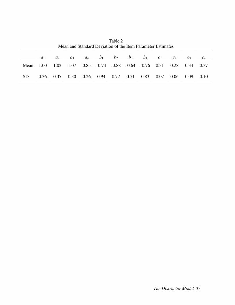
The mean and standard deviation of each of the a-, b-, and c-parameters taken across all

20 items are displayed in Table 2.

To gain a better understanding of the relationship between the estimated item

parameters and the form of the DM, the OCCs were plotted for several of the test items.

Figure 3 displays the OCCs for Item 6. Of particular interest for Item 6 is distractor 3,

which displayed a relatively high probability of selection for the θ range of -1 to -3. The

relatively high probability associated with distractor 3 in the θ range of -1 to -3 is

attributable to the relatively high discrimination of the third contrast function (a3 = -1.18)

coupled with the location of the third contrast function (b3 = -0.79) that sits far to the

right of the other contrast functions. In addition, the relatively low value of the c-

parameter for the third contrast function (c3 = 0.22) leads the probability of selecting the

third distractor to be above that of the other options at the lower levels of θ.

Figure 4 displays the OCCs for Item 11. For this item, distractor 1 had a relatively

high probability of selection in the θ range of -2 to -1, which is attributable to the

relatively high a- and b-parameters of the first contrast function (a1 = -1.12 and b1 = -

0.33). Also of interest is that distractor 3 reached a relatively high probability of selection


at the very low levels of θ, which is attributable to the relatively low value of the c-

parameter (c3 = 0.20).

Figure 5 displays the OCCs for Item 19, a relatively difficult item for which the

OCCs of the four distractors were determined largely by the c-parameters of their

respective contrast functions. In particular, for θ < 0, the ordering of the probability of

selection for the four distractors is inversely related to the c-parameter of the associated

contrast function: distractor 2 has the highest probability of selection and c2 = 0.19,

distractor 3 has the second highest probability of selection and c3 = 0.22, distractor 1 has

the third highest probability of selection and c1 = 0.27, and distractor 4 has the lowest

probability of selection (of the distractors) and c4 = 0.41. This item clearly illustrates the

utility of the c-parameter in the DM, and how the c-parameter is inversely related to the

probability of selection as θ becomes arbitrarily low.

Fit was examined by comparing the observed and expected proportion selecting

each response option within ten intervals along the latent continuum. The latent

continuum was placed on a standard metric (one logit equaled one unit on the latent

metric), and the ten intervals were 0.5 logits in length beginning at -2.5 and extending to

2.5 (i.e., -2.50 to -2.01, -2.00 to -1.51, …., 2.00 to 2.50). At the midpoint of each of the

ten intervals the expected proportion selecting each response option for the item in

question was computed, and compared to the observed proportions for the respondents in

the respective interval. The mean squared error for each response option was computed

by summing the squared differences between the expected and observed proportions, and

the RMSE for each response option was obtained by taking the square root of the mean

squared error. To obtain an index of fit across all response options, an aggregated RMSE


value was computed by considering the summated squared differences across all five

response options.

Upon examination of the data, only six observations were located in the lowest

interval (-2.5 to -2.01), and thus this interval was excluded from the computation of the

RMSE values. Table 2 displays the resulting values of RMSE for each response option,

and aggregated across all response options. The RMSE values were typically less than

0.05 for each distractor, providing evidence of relatively good fit. The values of RMSE

for the correct option tended to be slightly larger than those of the distractors, which is

likely attributable to the larger scale of the correct response; the correct response spans

probabilities from near zero to near unity, while the distractors typically span

probabilities from near zero to less than .5. The values of the aggregated RMSE taken

across all response options ranged between 0.018 and 0.043, which provides further

evidence of relatively good fit of the model to the data.

In addition to the RMSE values shown in Table 2, fit plots (plots of the expected

and observed proportion selecting each response option within each stratum) were

constructed for each item. The fit plots were visually inspected to identify items

displaying substantial lack of fit. Upon visual inspection of the fit plots, no items were

flagged as having substantial lack of fit.

Discussion

In this paper we proposed the distractor model (DM), an adaptation of Revuelta’s

(2005) DLT response model for multiple-choice items. The advantageous features of the

DM include: (a) the DM uses a parameterization that is consistent with that of the NRM;

(b) the DM uses fewer parameters than Thissen and Steinberg’s (1984) multiple-choice


response model; (c) the DM is based on contrast functions that are parameterized

according to a three-parameter logistic model that is similar to that commonly employed

for dichotomously scored items, and thus is based on a theory and form that is pervasive

in the IRT literature. The DM was applied to a 20-item test of multiple-choice items, and

the fit of the data to the DM was deemed good through visual inspection of fit plots.

These results suggest that the DM holds promise to being a viable alternative for

modeling multiple-choice item responses.

Adding the DM to the family of polytomous models appropriate for multiple-

choice item formats can serve several advantageous functions. First, the DM is based on

different model assumptions than the NRM and the MCM. In particular, the DM asserts

that each contrast function follows a three-parameter logistic form, which distinguishes it

from the NRM and the MCM. As a result, the DM offers a novel way to conceptualize,

model, and interpret responses to multiple-choice items. Second, because the assumptions

underlying the DM are different than those of the NRM and MCM, it offers an alternative

model to simulate responses to multiple-choice items. Being able to simulate data using a

variety of plausible models is a useful property of simulation studies evaluating models

for multiple-choice items.

While the DM incorporates a theory and parameterization for guessing in

multiple-choice items, additional research is required to evaluate whether the DM

provides better fit to multiple-choice item responses than other polytomous models such

as the NRM and the MCM. Previous research (Drasgow et al., 1995) found modest

differences in the fit of NRM and the MCM to multiple-choice items, and additional

research is required to evaluate whether the fit of the DM to real data is comparable to


that of the MCM and NRM. In addition, a comparison of the stability of the DM

parameter estimates to those of the MCM and NRM would be important in shedding light

on which model holds the greatest value across a range a conditions.


Appendix

)|()|(

)|(),,|(

�mYP�kYP

�kYPmkY�kYP

jj

jjj =+=

====

��

�

=′′′

=′′′

=′′′

+++++

++=

m

kkjkjjmjm

m

kkjkjjkjk

m

kkjkjjkjk

�ab�ab�ab�ab

�ab�ab

11

1

)exp()exp()exp()exp(

)exp()exp(

)exp()exp(

)exp(

�ab�ab

�ab

jmjmjkjk

jkjk

++++

=

)exp()exp(1

)exp()exp(

�ab�ab

�ab�ab

jmjmjkjk

jmjmjkjk

+++++

=

[ ][ ])()(exp1

)()(exp

jmjkjmjk

jmjkjmjk

aa�bb

aa�bb

−+−+

−+−=

)exp(1

)exp(**

**

�ab

�ab

jkjk

jkjk

+++

=


References

Birnbaum, A. (1968). Some latent trait models and their use in inferring an examinee’s

ability. In F. M. Lord and M. R. Novick, Statistical theories of mental test scores.

Reading, MA: Addison-Wesley.

Bock, R. D. (1972). Estimating item parameters and latent ability when responses

are scored in two or more nominal categories. Psychometrika, 37, 29-51.

Bock, R. D. (1997). The nominal categories model. In W. J. van der Linden & R. K.

Hambleton (Eds.), Handbook of modern item response theory (pp. 33-49). New

York: Springer.

Bock, R. D., & Aitkin, M. (1981). Marginal maximum likelihood estimation of item

parameters. An application of an EM algorithm. Psychometrika, 46, 443-459.

Brooks, S. P., & Gelman, A. (1998). General methods for monitoring convergence of

iterative simulations. Journal of Computational and Graphical Statistics, 7, 434-

455.

Casella, G., & George, E. I. (1995). Explaining the Gibbs sampler. The American

Statistician, 46, 167-174. Chib, S., & Greenberg, E. (1995). Understanding the

Metropolis-Hastings algorithm. The American Statistician, 49, 327-335.

Chib, S., & Greenberg, E. (1995). Understanding the Metropolis-Hastings algorithm. The

American Statistician, 49, 327-335.

De Ayala, R. J. (1989). A comparison of the nominal response model and the three-

parameter logistic model in computerized adaptive testing. Educational and

Psychological Measurement, 49, 789-805.

De Ayala, R. J. (1992). The nominal response model in computerized adaptive testing.


Applied Psychological Measurement, 16, 327-343.

De Ayala, R. J., & Sava-Bolesta, M. (1999). Item parameter recovery for the nominal

response model. Applied Psychological Measurement, 23, 3-19.

DeMars, C. E. (2003). Sample size and recovery of nominal response model item

parameters. Applied Psychological Measurement, 27, 275-288.

Doornik, J. A. (2003). Object-Oriented Matrix Programming using Ox (Version 3.1)

[Computer software]. London: Timberlake Consultants Press.

Drasgow, F., Levine, M. V., Tsien, S., Williams, B., & Mead, A. (1995). Fitting

polytomous item response theory models to multiple-choice tests. Applied


Gamerman, D. (1997). Markov chain Monte Carlo: Stochastic simulation for Bayesian

inference. London: Chapman & Hall.

Gelman, A., Carlin, J. B., Stern, H. S., & Rubin, R. B. (2003). Bayesian data analysis

(2nd ed.). London: Chapman & Hall.

Gilks, W. R., Richardson, S., & Spiegelhalter, D. J. (1996). Introducing Markov chain

Monte Carlo. In W. R. Gilks, S. Richardson, &D. J. Spiegelhalter (Eds.), Markov

chain Monte Carlo in practice (pp. 1-17). London: Chapman & Hall.

Lord, F.M. (1980). Applications of item response theory to practical testing problems.

NJ: Lawrence Erlbaum.

Osterlind, S. J. (1998). Constructing test items: Multiple-choice, constructed response,

performance, and other formats (2nd ed.). Boston: Kluwer Academic.


Patz, R. J., & Junker, B. W. (1999a). Applications and extensions of MCMC in IRT:

Multiple item types, missing data, and rated responses. Journal of Educational

and Behavioral Statistics, 24, 342-366.

Patz, R. J., & Junker, B. W. (1999b). A straightforward approach to Markov chain Monte

Carlo methods for item response theory. Journal of Educational and Behavioral

Statistics, 24, 146-178.

Rasch, G. (1960). Probabilistic models for some intelligence and attainment tests.

Copenhagen, Denmark:Danmarks Paedogogiske Institut.

Revuelta, J. (2005). An item response model for nominal data based on the rising

selection ratios criterion. Psychometrika, 70, 305-324.

Roberts, J. S., Donoghue, J. R, & Laughlin, J. E. (2000). A general item response theory

model for unfolding unidimensional polytomous responses. Applied


Samejima, F. (1979). A new family of models for the multiple choice item. (Research

Report No. 79-4) Knoxville: University of Tennessee, Department of Psychology.

Thissen, D. (1976). Information in wrong responses to Raven’s Progressive Matrices.

Journal of Educational Measurement, 13, 201-214.

Thissen, D., & Steinberg, L. (1984). A response model for multiple choice items.

Psychometrika, 49, 501-519.

Thissen, D., & Steinberg, L. (1997). A response model for multiple-choice items. In W. J.

van der Linden & R. K. Hambleton (Eds.), Handbook of modern item response

theory (pp. 51-65). New York: Springer.

Thissen, D., Steinberg, L., & Fitzpatrick, A. R. (1989). Multiple-choice items: The


distractors are also part of the item. Journal of Educational Measurement, 26,

161-176.

Tierney, L. (1994). Markov chains for exploring posterior distributions (with discussion).

Annals of Statistics, 22, 1701-1762.

University of Wisconsin Center for Placement Testing (2006). University of Wisconsin

Mathematics Placement Test (Form 06X). Madison, WI: Author.


Author Note

The authors would like to thank Alan Cohen and James Wollack for their assistance in

obtaining the data used in the applied example of this paper.


Table 1 Item Parameter Estimates and Estimated Standard Errors

Item

a1

a2

a3

a4

b1

b2

b3

b4

c1

c2

c3

c4

1 -0.57 (0.05)

-0.81 (0.10)

-1.14 (0.15)

-0.52 (0.02)

-2.57 (0.27)

-1.90 (0.30)

-0.35 (0.14)

-0.75 (0.14)

0.32 (0.12)

0.26 (0.14)

0.46 (0.04)

0.47 (0.03)

2 -1.78 (0.15)

-1.15 (0.13)

-1.05 (0.13)

-1.37 (0.20)

-0.29 (0.08)

-0.23 (0.11)

-1.39 (0.24)

-0.64 (0.15)

0.35 (0.05)

0.21 (0.06)

0.23 (0.13)

0.44 (0.06)

3 -0.57 (0.06)

-1.02 (0.14)

-1.01 (0.14)

-0.83 (0.12)

-0.33 (0.29)

-0.98 (0.22)

-0.50 (0.20)

-1.38 (0.32)

0.40 (0.08)

0.40 (0.09)

0.43 (0.07)

0.37 (0.12)

4 -1.48 (0.21)

-1.53 (0.18)

-1.63 (0.19)

-0.66 (0.11)

-0.06 (0.11)

-0.22 (0.10)

-0.11 (0.10)

0.35 (0.24)

0.45 (0.04)

0.29 (0.05)

0.32 (0.05)

0.31 (0.07)

5 -0.84 (0.14)

-0.98 (0.15)

-0.78 (0.13)

-0.65 (0.10)

-0.16 (0.23)

-0.19 (0.20)

-0.33 (0.29)

0.12 (0.27)

0.24 (0.09)

0.30 (0.08)

0.40 (0.09)

0.41 (0.07)

6 -1.47 (0.24)

-1.06 (0.13)

-1.18 (0.13)

-0.81 (0.11)

-2.06 (0.25)

-1.36 (0.22)

-0.79 (0.16)

-2.10 (0.31)

0.29 (0.14)

0.29 (0.13)

0.22 (0.09)

0.24 (0.14)

7 -0.94 (0.16)

-1.47 (0.19)

-1.21 (0.17)

-0.72 (0.09)

-0.46 (0.31)

-0.42 (0.12)

-1.07 (0.21)

-0.17 (0.21)

0.36 (0.12)

0.27 (0.07)

0.30 (0.12)

0.18 (0.08)

8 -0.80 (0.11)

-1.16 (0.15)

-0.80 (0.13)

-0.80 (0.13)

-0.61 (0.24)

0.20 (0.10)

-0.83 (0.33)

0.15 (0.20)

0.18 (0.10)

0.24 (0.04)

0.33 (0.12)

0.46 (0.05)

9 -1.19 (0.18)

-0.65 (0.08)

-0.77 (0.10)

-0.87 (0.12)

-0.49 (0.20)

-1.69 (0.36)

-1.28 (0.30)

-0.51 (0.23)

0.35 (0.09)

0.24 (0.15)

0.38 (0.11)

0.43 (0.07)

10 -1.30 (0.18)

-1.05 (0.13)

-1.78 (0.15)

-1.10 (0.15)

-0.90 (0.19)

-1.05 (0.23)

-0.83 (0.09)

-1.39 (0.25)

0.38 (0.10)

0.29 (0.12)

0.44 (0.05)

0.36 (0.12)

11 -1.12 (0.13)

-0.70 (0.09)

-0.71 (0.09)

-1.14 (0.16)

-0.33 (0.12)

-2.14 (0.33)

-0.91 (0.29)

-0.96 (0.20)

0.23 (0.06)

0.26 (0.14)

0.20 (0.12)

0.44 (0.07)

12 -0.58 (0.05)

-0.91 (0.11)

-0.85 (0.11)

-1.13 (0.13)

-2.26 (0.32)

-1.55 (0.27)

-1.06 (0.28)

-0.73 (0.16)

0.26 (0.14)

0.28 (0.13)

0.37 (0.11)

0.42 (0.07)

13 -0.70 (0.08)

-0.87 (0.12)

-1.16 (0.15)

-0.66 (0.09)

-1.67 (0.33)

-1.13 (0.30)

-0.55 (0.14)

-2.11 (0.37)

0.29 (0.14)

0.34 (0.13)

0.45 (0.05)

0.32 (0.14)

14 -1.41 (0.20)

-1.81 (0.13)

-1.35 (0.20)

-0.98 (0.10)

-0.60 (0.17)

-0.52 (0.09)

-0.55 (0.18)

-0.35 (0.12)

0.31 (0.10)

0.31 (0.06)

0.36 (0.09)

0.13 (0.06)

15 -1.22 (0.15)

-0.55 (0.04)

-1.11 (0.25)

-0.60 (0.08)

0.75 (0.08)

0.32 (0.25)

1.07 (0.14)

-0.21 (0.24)

0.28 (0.02)

0.44 (0.05)

0.46 (0.03)

0.45 (0.05)

16 -0.86 (0.15)

-0.67 (0.09)

-0.77 (0.12)

-0.65 (0.08)

0.52 (0.16)

-1.75 (0.38)

-2.29 (0.35)

-1.53 (0.35)

0.29 (0.06)

0.31 (0.14)

0.31 (0.13)

0.32 (0.13)

17 -0.52 (0.02)

-0.69 (0.08)

-0.84 (0.10)

-0.51 (0.01)

-2.22 (0.27)

-1.49 (0.33)

-1.07 (0.24)

0.11 (0.13)

0.38 (0.10)

0.24 (0.14)

0.21 (0.11)

0.49 (0.01)

18 -0.87 (0.12)

-0.75 (0.11)

-0.85 (0.14)

-0.73 (0.10)

-0.90 (0.27)

-0.54 (0.28)

-0.32 (0.27)

-2.47 (0.31)

0.37 (0.11)

0.24 (0.11)

0.33 (0.10)

0.27 (0.14)

19 -1.17 (0.17)

-1.81 (0.13)

-1.38 (0.19)

-1.36 (0.23)

0.07 (0.14)

0.41 (0.05)

0.59 (0.08)

0.11 (0.15)

0.27 (0.06)

0.19 (0.02)

0.22 (0.03)

0.41 (0.06)

20 -0.69 (0.11)

-0.76 (0.10)

-1.00 (0.14)

-1.02 (0.14)

-0.26 (0.28)

-1.30 (0.31)

-0.20 (0.18)

-0.70 (0.21)

0.23 (0.10)

0.25 (0.14)

0.31 (0.07)

0.41 (0.08)

Note. Values in parentheses correspond to the estimated standard error of the parameter estimate.


Table 2 Mean and Standard Deviation of the Item Parameter Estimates

a1

a2

a3

a4

b1

b2

b3

b4

c1

c2

c3

c4

Mean 1.00 1.02 1.07 0.85 -0.74 -0.88 -0.64 -0.76 0.31 0.28 0.34 0.37

SD 0.36 0.37 0.30 0.26 0.94 0.77 0.71 0.83 0.07 0.06 0.09 0.10


Table 3 RMSE Values for Each Response Option

Response Option

Item

1

2

3

4

5

Aggregated

1 0.032 0.038 0.010 0.047 0.045 0.037 2 0.015 0.031 0.047 0.009 0.022 0.028 3 0.027 0.010 0.028 0.015 0.030 0.024 4 0.013 0.022 0.014 0.027 0.033 0.023 5 0.027 0.018 0.016 0.023 0.047 0.029 6 0.025 0.019 0.025 0.016 0.050 0.030 7 0.015 0.012 0.023 0.031 0.042 0.027 8 0.028 0.032 0.017 0.026 0.033 0.028 9 0.012 0.016 0.013 0.015 0.042 0.022 10 0.011 0.019 0.009 0.005 0.033 0.018 11 0.021 0.011 0.036 0.019 0.047 0.030 12 0.020 0.027 0.011 0.031 0.027 0.024 13 0.015 0.015 0.016 0.013 0.041 0.023 14 0.043 0.038 0.018 0.039 0.034 0.035 15 0.029 0.050 0.027 0.021 0.068 0.043 16 0.034 0.007 0.019 0.033 0.050 0.032 17 0.016 0.017 0.036 0.053 0.068 0.043 18 0.015 0.028 0.023 0.010 0.041 0.026 19 0.016 0.020 0.034 0.012 0.035 0.025 20 0.056 0.014 0.019 0.012 0.051 0.036 Note. Response options 1, 2, 3, and 4 correspond to distractors. Option 5 is the correct response. The aggregated column corresponds to the RMSE aggregated across all five response options.


Figure 1

Contrast Functions for a Hypothetical Four-Option Multiple-Choice Item Parameterized

According to the DM

0

0.25

0.5

0.75

1

-3 -2 -1 0 1 2 3

Latent Trait

P(C

ontr

ast)

CF-1

CF-2

CF-3

Note. The three contrast functions are labeled CF-1 (contrasts distractor 1 and the correct

option), CF-2 (contrasts distractor 2 and the correct option), and CF-3 (contrasts

distractor 3 and the correct option). The three contrast functions have parameters: a1 = -

1.5, a2 = -1, a3 = -1, b1 = -1, b2 = 0, b3 = 1, c1 = 0.2, c2 = 0.5, c3 = 0.3.


Figure 2

Option Characteristic Curves for a Hypothetical Four-Option Multiple-Choice Item

Parameterized According to the DM

0

0.25

0.5

0.75

1

-3 -2 -1 0 1 2 3

Latent Trait

P(Y

)

1

2

3

4

Note. The DM parameters are: a1 = -1.5, a2 = -1, a3 = -1, b1 = -1, b2 = 0, b3 = 1, c1 = 0.2,

c2 = 0.5, c3 = 0.3. Option 4 corresponds to the correct option.


Figure 3

Option Characteristic Curves for Item 6 of the Algebra Test

0

0.25

0.5

0.75

1

-3 -2 -1 0 1 2 3

Latent Trait

P(Y

)

1

2

3

4

5

Note. The DM parameters are: a1 = -1.47, a2 = -1.06, a3 = -1.18, a4 = -0.81, b1 = -2.06, b2

= -1.36, b3 = -0.79, b4 = -2.10, c1 = 0.29, c2 = 0.29, c3 = 0.22, c4 = 0.24. Option 5

corresponds to the correct option.


Figure 4


0

0.25

0.5

0.75

1

-3 -2 -1 0 1 2 3

Latent Trait

P(Y

)

1

2

3

4

5

Note. The DM parameters are: a1 = -1.12, a2 = -0.70, a3 = -0.71, a4 = -1.14, b1 = -0.33, b2

= -2.14, b3 = -0.91, b4 = -0.96, c1 = 0.23, c2 = 0.26, c3 = 0.20, c4 = 0.44. Option 5



Figure 5


0

0.25

0.5

0.75

1

-3 -2 -1 0 1 2 3

Latent Trait

P(Y

)

1

2

3

4

5

Note. The DM parameters are: a1 = -1.17, a2 = -1.81, a3 = -1.38, a4 = -1.36, b1 = 0.07, b2

= 0.41, b3 = 0.59, b4 = 0.11, c1 = 0.27, c2 = 0.19, c3 = 0.22, c4 = 0.41. Option 5


A New Response Model for Multiple-Choice Items Randall D ...

Documents

Transcript of A New Response Model for Multiple-Choice Items Randall D ...