A New QEA Computing Near-Optimal Low-Discrepancy · PDF fileA New QEA Computing Near-Optimal...
13
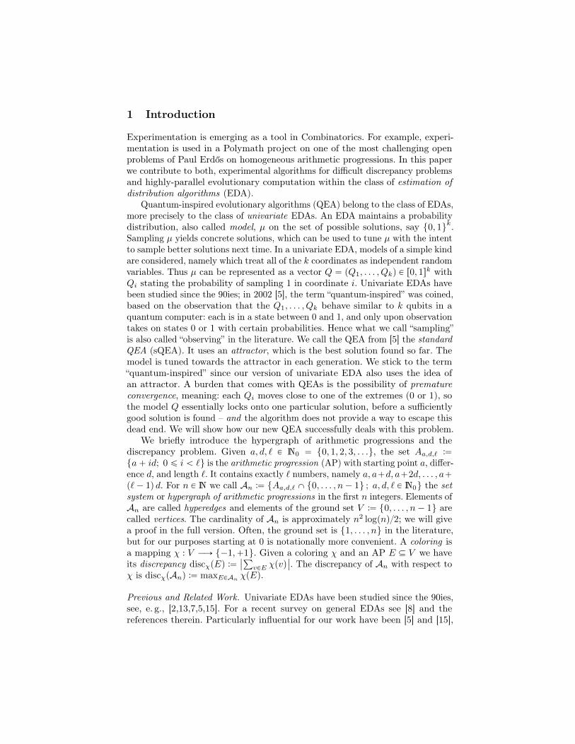
A New QEA Computing Near-Optimal Low-Discrepancy Colorings in the Hypergraph of Arithmetic Progressions Lasse Kliemann 1 , Ole Kliemann 1 , C. Patvardhan 2 , Volkmar Sauerland 1 , and Anand Srivastav 1 1 Christian-Albrechts-Universität zu Kiel Institut für Informatik Christian-Albrechts-Platz 4 24118 Kiel, Germany contact: [email protected] 2 Dayalbagh Educational Institute Deemed University Agra, India [email protected] Bibliographic reference: V. Bonifaci, C. Demetrescu, A. Marchetti-Spaccamela (Eds.): SEA 2013, LNCS 7933, pp. 67-78, 2013. c Springer-Verlag Berlin Heidelberg 2013. The original publication is available at www.springerlink.com. http://dx.doi.org/10.1007/978-3-642-38527-8_8 Abstract. We present a new quantum-inspired evolutionary algorithm, the attractor population QEA (apQEA). Our benchmark problem is a classical and difficult problem from Combinatorics, namely finding low-discrepancy colorings in the hypergraph of arithmetic progressions on the first n integers, which is a massive hypergraph (e. g., with ap- prox. 3.88 ˆ 10 11 hyperedges for n “ 250 000). Its optimal low-discrepancy coloring bound Θp 4 √ nq is known and it has been a long-standing open problem to give practically and/or theoretically efficient algorithms. We show that apQEA outperforms known QEA approaches and the classical combinatorial algorithm (Sárközy 1974) by a large margin. Regarding practicability, it is also far superior to the SDP-based polynomial-time algorithm of Bansal (2010), the latter being a breakthrough work from a theoretical point of view. Thus we give the first practical algorithm to construct optimal colorings in this hypergraph, up to a constant fac- tor. We hope that our work will spur further applications of Algorithm Engineering to Combinatorics. Keywords: estimation of distribution algorithm, quantum-inspired evolu- tionary algorithm, hypergraph coloring, arithmetic progressions, algorithm engineering, combinatorics
Transcript of A New QEA Computing Near-Optimal Low-Discrepancy · PDF fileA New QEA Computing Near-Optimal...
A New QEA Computing Near-OptimalLow-Discrepancy Colorings in the Hypergraph of
Arithmetic Progressions
Lasse Kliemann1, Ole Kliemann1, C. Patvardhan2, Volkmar Sauerland1, andAnand Srivastav1
1 Christian-Albrechts-Universität zu KielInstitut für Informatik
Christian-Albrechts-Platz 424118 Kiel, Germany
contact: [email protected] Dayalbagh Educational Institute
Deemed UniversityAgra, India
Bibliographic reference:
V. Bonifaci, C. Demetrescu, A. Marchetti-Spaccamela (Eds.):SEA 2013, LNCS 7933, pp. 67-78, 2013.c© Springer-Verlag Berlin Heidelberg 2013.The original publication is available at www.springerlink.com.http://dx.doi.org/10.1007/978-3-642-38527-8_8
Abstract. We present a new quantum-inspired evolutionary algorithm,the attractor population QEA (apQEA). Our benchmark problem isa classical and difficult problem from Combinatorics, namely findinglow-discrepancy colorings in the hypergraph of arithmetic progressionson the first n integers, which is a massive hypergraph (e. g., with ap-prox. 3.88ˆ1011 hyperedges for n “ 250 000). Its optimal low-discrepancycoloring bound Θp 4
√nq is known and it has been a long-standing open
problem to give practically and/or theoretically efficient algorithms. Weshow that apQEA outperforms known QEA approaches and the classicalcombinatorial algorithm (Sárközy 1974) by a large margin. Regardingpracticability, it is also far superior to the SDP-based polynomial-timealgorithm of Bansal (2010), the latter being a breakthrough work froma theoretical point of view. Thus we give the first practical algorithmto construct optimal colorings in this hypergraph, up to a constant fac-tor. We hope that our work will spur further applications of AlgorithmEngineering to Combinatorics.
Keywords: estimation of distribution algorithm, quantum-inspired evolu-tionary algorithm, hypergraph coloring, arithmetic progressions, algorithmengineering, combinatorics
1 Introduction
Experimentation is emerging as a tool in Combinatorics. For example, experi-mentation is used in a Polymath project on one of the most challenging openproblems of Paul Erdős on homogeneous arithmetic progressions. In this paperwe contribute to both, experimental algorithms for difficult discrepancy problemsand highly-parallel evolutionary computation within the class of estimation ofdistribution algorithms (EDA).
Quantum-inspired evolutionary algorithms (QEA) belong to the class of EDAs,more precisely to the class of univariate EDAs. An EDA maintains a probabilitydistribution, also called model, µ on the set of possible solutions, say 0, 1k.Sampling µ yields concrete solutions, which can be used to tune µ with the intentto sample better solutions next time. In a univariate EDA, models of a simple kindare considered, namely which treat all of the k coordinates as independent randomvariables. Thus µ can be represented as a vector Q “ pQ1, . . . , Qkq P r0, 1s
k withQi stating the probability of sampling 1 in coordinate i. Univariate EDAs havebeen studied since the 90ies; in 2002 [5], the term “quantum-inspired” was coined,based on the observation that the Q1, . . . , Qk behave similar to k qubits in aquantum computer: each is in a state between 0 and 1, and only upon observationtakes on states 0 or 1 with certain probabilities. Hence what we call “sampling”is also called “observing” in the literature. We call the QEA from [5] the standardQEA (sQEA). It uses an attractor, which is the best solution found so far. Themodel is tuned towards the attractor in each generation. We stick to the term“quantum-inspired” since our version of univariate EDA also uses the idea ofan attractor. A burden that comes with QEAs is the possibility of prematureconvergence, meaning: each Qi moves close to one of the extremes (0 or 1), sothe model Q essentially locks onto one particular solution, before a sufficientlygood solution is found – and the algorithm does not provide a way to escape thisdead end. We will show how our new QEA successfully deals with this problem.
We briefly introduce the hypergraph of arithmetic progressions and thediscrepancy problem. Given a, d, ` P N0 “ 0, 1, 2, 3, . . ., the set Aa,d,` :“a` id; 0 ď i ă ` is the arithmetic progression (AP) with starting point a, differ-ence d, and length `. It contains exactly ` numbers, namely a, a`d, a`2d, . . . , a`p`´ 1q d. For n P N we call An :“ Aa,d,` X 0, . . . , n´ 1 ; a, d, ` P N0 the setsystem or hypergraph of arithmetic progressions in the first n integers. Elements ofAn are called hyperedges and elements of the ground set V :“ 0, . . . , n´ 1 arecalled vertices. The cardinality of An is approximately n2 logpnq2; we will givea proof in the full version. Often, the ground set is 1, . . . , n in the literature,but for our purposes starting at 0 is notationally more convenient. A coloring isa mapping χ : V ÝÑ ´1,`1. Given a coloring χ and an AP E Ď V we haveits discrepancy discχpEq :“
∣∣∑vPE χpvq
∣∣. The discrepancy of An with respect toχ is discχpAnq :“ maxEPAn χpEq.
Previous and Related Work. Univariate EDAs have been studied since the 90ies,see, e. g., [2,13,7,5,15]. For a recent survey on general EDAs see [8] and thereferences therein. Particularly influential for our work have been [5] and [15],
where sQEA and vQEA are presented, respectively. vQEA extends the attractorconcept in a way to allow for better exploration. But for the discrepancy problem,vQEA is not well suited for reasons explained later. In recent years, variants ofQEAs have been successfully used on benchmark as well as on difficult practiceproblems, see, e. g., [1,10,11,14,6].
For An, in 1964, it was shown by Roth [16] that there is no coloring withdiscrepancy below Ωp 4
√nq. More than 20 years later, it was shown by Matoušek
and Spencer [12] that there exists a coloring with discrepancy Op 4√nq, so together
with the earlier result we have Θp 4√nq. The proof is non-constructive, and
the problem of efficiently computing such colorings remained open. For manyyears, Sárközy’s approximation algorithm (see [4]) was the best known, provablyattaining discrepancy Op 3
√n logpnqq; experiments suggest that (asymptotically)
it does not perform better than this guarantee. Recently, in a pioneering work, theproblem was solved by Bansal [3], using semi-definite programs (SDP). However,Bansal’s algorithm requires solving a series of SDPs that grow in the number ofhyperedges, making it practically problematic for An. In our experiments, even forn ă 100, it requires several hours to complete, whereas our apQEA (in a parallelimplementation) only requires a couple of minutes up to n “ 100 000. Computingoptimal low-discrepancy colorings for general hypergraphs is NP-hard [9].
Our Contribution. We use the problem of computing low-discrepancy coloringsin An in order to show limitations of sQEA and how a new form of QEAcan successfully overcome these limitations. Our new QEA uses an attractorpopulation where the actual attractor is repeatedly selected from. We call itattractor population QEA (apQEA). The drawback of sQEA appears to bepremature convergence, or in other words, a lack of exploration of the searchspace. We show that even by reducing the learning rate drastically in sQEA andby using local and global migration, it does not attain the speed and solutionquality of apQEA. In addition to the exploration capabilities of apQEA, we showthat – with an appropriate tuning of parameters – it scales well in the number ofparallel processors: when doubling the number of processor cores from 96 to 192,running times reduces to roughly between 40% and 60%.
We also look at the combinatorial structure of An. Based on an idea bySárközy (see [4]) we devise a modulo coloring scheme, resulting in a search spacereduction and faster fitness function evaluation. This, together with apQEA,allows us to compute low-discrepancy colorings that are optimal up to a constantfactor, in the range up to n “ 250 000 vertices. For this n, the cardinality ofAn is approx. 3.88 ˆ 1011, which means a massive hypergraph. Precisely, wecompute colorings with discrepancy not more than 3 4
√n; we call b3 4
√nc the target
discrepancy. We have chosen factor 3, because this appeared as an attainable goalin reasonable time in preliminary experiments. Better approximations may bepossible with other parameters and more processors and/or more time. Coloringsfound by our algorithm can be downloaded3 and easily verified.
3 http://www.informatik.uni-kiel.de/~lki/discap-results.tar.xz
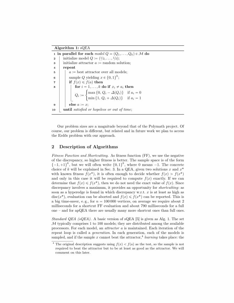
Algorithm 1: sQEA1 in parallel for each model Q “ pQ1, . . . , Qkq PM do2 initialize model Q :“ p12, . . . , 12q;3 initialize attractor a :“ random solution;4 repeat5 a :“ best attractor over all models;6 sample Q yielding x P 0, 1k;7 if fpxq ď fpaq then8 for i “ 1, . . . , k do if xi ‰ ai then
Qi :“
max 0, Qi ´∆pQiq if ai “ 0
min 1, Qi `∆pQiq if ai “ 1
9 else a :“ x;10 until satisfied or hopeless or out of time;
Our problem sizes are a magnitude beyond that of the Polymath project. Ofcourse, our problem is different, but related and in future work we plan to accessthe Erdős problem with our approach.
2 Description of Algorithms
Fitness Function and Shortcutting. As fitness function (FF), we use the negativeof the discrepancy, so higher fitness is better. The sample space is of the form´1,`1k, but we will often write 0, 1k, where 0 means ´1. The concretechoice of k will be explained in Sec. 3. In a QEA, given two solutions x and x˚with known fitness fpx˚q, it is often enough to decide whether fpxq ą fpx˚qand only in this case it will be required to compute fpxq exactly. If we candetermine that fpxq ď fpx˚q, then we do not need the exact value of fpxq. Sincediscrepancy involves a maximum, it provides an opportunity for shortcutting : assoon as a hyperedge is found in which discrepancy w.r.t. x is at least as high asdiscpx˚q, evaluation can be aborted and fpxq ď fpx˚q can be reported. This isa big time-saver, e. g., for n “ 100 000 vertices, on average we require about 2milliseconds for a shortcut FF evaluation and about 790 milliseconds for a fullone – and for apQEA there are usually many more shortcut ones than full ones.
Standard QEA (sQEA). A basic version of sQEA [5] is given as Alg. 1. The setM typically comprises 1 to 100 models; they are distributed among the availableprocessors. For each model, an attractor a is maintained. Each iteration of therepeat loop is called a generation. In each generation, each of the models issampled, and if the sample x cannot beat the attractor,4 learning takes place: the4 The original description suggests using fpxq ă fpaq as the test, so the sample is notrequired to beat the attractor but to be at least as good as the attractor. We willcomment on this later.
model is shifted slightly towards a, where x and a differ. Linear learning meansusing a fixed amount, e. g., ∆pQiq “ ∆ “ 1
100 . In [5,15] rotation learning is used:the point p
√1´Qi,
√Qiq in the plane is rotated either clockwise (if ai “ 0) or
counter-clockwise (if ai “ 1), and the new value of Qi becomes the square root ofthe new ordinate. This is inspired by quantum computing; an actual benefit couldbe that towards the extremes (0 and 1) shifts become smaller. We will test sQEAand vQEA with linear as well as rotation learning and stick to linear learning forapQEA. The learning resolution gives the number of possible values that each Qican assume inside r0, 1s. For linear learning, this is 1
∆ . For rotation learning, thisis determined by the angle by which we rotate; it is typically between 0.01π and0.001π. Since the interval is r0, π2s, this means a learning resolution between 50and 500. As an extension, multiple samples can be taken in line 6 and the modelis only shifted if none of them beats the attractor (an arbitrary one of them ischosen for the test xi ‰ ai). If one of the samples beats the attractor, the bestone is used to update the attractor in line 9. We always use 10 samples.
What happens in line 5 is called synchronization or migration. Anotherextension, intended to prevent premature convergence, is the use of local andglobal migration. Models are bundled into groups, and the attractor of a modelQ is set to the best attractor over all models in Q’s group (local migration).Only every Tg generations, the best attractor over all models is used (globalmigration). We call Tg the global migration period.
The repeat loop stops when we are “satisfied or hopeless or out of time”.We are satisfied in the discrepancy problem when the discrepancy is lesser orequal to 3 4
√n. A possible criterion for hopelessness is when all the models have
only very little entropy left. Entropy is a measure of randomness, defined as∑ki“1´ logpQiq, which is at its maximum k when Qi “
12 for all i, and at its
minimum 0 if Qi P 0, 1 for all i. In all our experiments with sQEA, we willimpose a simple time limit guided by the times needed by apQEA.
Versatile QEA (vQEA). vQEA [15] works similar to sQEA with the exceptionthat the attractor update in line 9 is carried out unconditionally. The descriptiongiven in [15] states that the attractor of each model in generation t` 1 is the bestsample from generation t, over all models. This means that parallel processeshave to synchronize after each generation. and also that at least one sample pergeneration must be fully evaluated, so only limited use of shortcutting is possible.
Attractor Population QEA (apQEA). Our new QEA, the apQEA, is given asAlg. 2. It strikes a balance between the approaches of sQEA and vQEA. InsQEA, the attractor essentially follows the best solution and only changes whenbetter solutions are found, while in vQEA the attractor changes frequently andis also allowed to assume inferior solutions. In apQEA, the attractor populationP is a set of solutions. From it, attractors are selected, e. g., using tournamentselection. When a sample cannot improve the population (fpxq ď f0) the modelis adjusted. Otherwise the solution is injected into the population. The numberof generations that a particular attractor stays in function is called the attractorpersistence; we fix it to 10 in all our experiments. Note that apQEA will benefit

Algorithm 2: apQEA
1 randomly initialize attractor population P Ď 0, 1k of cardinality S;2 in parallel for each model Q “ pQ1, . . . , Qkq PM do3 initialize model Q :“ p12, . . . , 12q;4 repeat5 a :“ select from P;6 do 10 times7 f0 :“ worst fitness in P;8 sample Q yielding x P 0, 1k;9 if fpxq ď f0 then
10 for i “ 1, . . . , k do if xi ‰ ai then
Qi :“
max 0, Qi ´∆pQiq if ai “ 0
min 1, Qi `∆pQiq if ai “ 1
11 else12 inject x into P;13 trim P to the size of S, removing worst solutions;
14 until satisfied or hopeless or out of time;
from shortcutting since fpxq has only to be computed when fpxq ą f0. Notealso that it is appropriate to treat the models asynchronously in apQEA, hencepreventing idle time: the attractor population is there, any process may injectinto it or select from it at any time (given an appropriate implementation).
A very important parameter is the size S of the population. We will see inexperiments that larger S means better exploration abilities. For the discrepancyproblem, we will have to increase S (moderately) when n increases.
Since the attractor changes often in apQEA, entropy oftentimes never reachesnear zero but instead oscillates around values like 20 or 30. A more stablemeasure is the mean Hamming distance in the attractor population, i. e., 1
(S2)¨∑
x,x1P(P2) |i; xi ‰ x1i|. However, it also can get stuck well above zero. Todetermine a hopeless situation, we instead developed the concept of a flatline.A flatline is a period of time in which neither the mean Hamming distance reachesa new minimum nor a better solution is found. When we encounter a flatlinestretching over 25% of the total running time so far, we declare the situationhopeless. To avoid erroneously aborting in early stages, we additionally demandthat the relative mean Hamming distance, which is the mean Hamming distancedivided by k, falls below 110. Those thresholds were found to be appropriate (forthe discrepancy problem) in preliminary experiments.
3 Modulo Coloring
Let p ď n be an integer. Given a partial coloring χ1 : 0, . . . , p´ 1 ÝÑ ´1,`1,i. e., a coloring of the first p vertices, we can construct a coloring χ by repeatingχ1, i. e., χ : V ÝÑ ´1,`1 , v ÞÑ χ1pv mod pq. We call χ1 a generating coloring.This way of coloring, with an appropriate p, brings many benefits. DenoteEp :“ A0,1,p “ 0, . . . , p´ 1, this is an AP and also the whole set on which χ1lives. Assume that χ1 is balanced, i. e., discχ1pEpq ď 1. Let Aa,d,` be any AP and` “ qp` r with integers q, r and r ă p. Then we have the decomposition:
Aa,d,` “q´1
⊍i“0
Aa`ipd,d,p︸ ︷︷ ︸Bi:“
YAa`qpd,d,r︸ ︷︷ ︸Bq :“
. (1)
Assuming p is prime, we have Bi mod p :“ v mod p; v P Bi “ Ep for eachi “ 0, . . . , q ´ 1, so discχpBiq “ discχ1pEpq ď 1. It follows discχpAa,d,`q ďq discχ1pEpq ` discχpBqq ď q ` discχpBqq. This is one of the essential ideas howSárközy’s Op 3
√n logpnqq bound is proved and it gives us a hint (which was
confirmed in experiments) that modulo colorings, constructed from balancedones, might tend to have low discrepancy. It is tempting to choose p very small,but the best discrepancy we can hope for when coloring modulo p is dnpe. Sincewe aim for 3 4
√n, we choose p as a prime number so that dnpe is some way below
3 4√n, precisely we choose p prime with np « 52 ¨ 4
√n, i. e., p « 25 ¨ n34.
Constructing balanced colorings is straightforward. Define h :“ p`12 (so
h “ Θpn34q) and let x P ´1,`1h. Then px1, . . . , xh´1,´xh´1, . . . ,´x1, xhqdefines a balanced coloring of Ep. We could have chosen different ways of orderingthe entries of x and their negatives, but this mirroring construction has shownto work best so far. We additionally alternate the last entry xh, so we use thefollowing generating coloring of length 2p:
px1, . . . , xh´1,´xh´1, . . . ,´x1, xh, x1, . . . , xh´1,´xh´1, . . . ,´x1,´xhq . (2)
Modulo coloring has further benefits. It reduces the search space from´1,`1n to ´1,`1h, where h “ Θpn34q. Moreover, it allows a much fasterFF evaluation: we can restrict to those Aa,d,` with a ď 2p´ 1. We also make useof a decomposition similar to (1), but which is more complicated since we exploitthe structure of (2); details will be given in the full version. We omit APs whichare too short to bring discrepancy above the target, giving additional speedup.
4 Experiments and Results
Implementation and Setup. To fully benefit from the features of apQEA, weneeded an implementation which allows asynchronous communication betweenprocesses. Our MPI-based implementations (version 1.2.4) exhibited unacceptableidle times when used for asynchronous communication, so we wrote our ownclient-server-based parallel framework. It consists of a server process that managesthe attractor population. Clients can connect to it at any time via TCP/IP and

do selection and injection; the server takes care of trimming the populationafter injection. Great care was put into making the implementation free of raceconditions. Most parts of the software is written in Bigloo5, an implementationof the Scheme programming language. The FF and a few other parts are writtenin C, for performance reasons and to have OpenMP available. OpenMP is used todistribute FF evaluation across multiple processor cores. So we have a two-levelparallelization: on the higher level, we have multiple processes treating multiplemodels and communicating via the attractor population server. On the lowerlevel, we have thread parallelization for the FF. The framework provides alsomeans to run sQEA and vQEA. We always use 8 threads (on 8 processor cores)for the FF. If not stated otherwise, a total of 96 processor cores is used. Thisallows us to have 12 models fully in parallel; if we use more models then the set ofmodels is partitioned and the models from each partition are treated sequentially.Experiments are carried out on the NECTM Linux Cluster of the Rechenzentrumat Kiel University, with SandyBridge-EPTM processors.
Results for sQEA. Recall the important parameters of sQEA: number of mod-els M , learning resolution R, global migration period Tg, and number of groups.For R, we use 50, 100 and 500, which are common settings, and also try 1000,2000, and 3000. In [6], it is proposed to choose Tg in linear dependence on R,which in our notation and neglecting the small additive constant reads Tg “ 2Rλwith 1.15 ď λ ď 1.34. We use λ “ 1.25 and λ “ 1.5, so Tg “ 2.5R and Tg “ 3R.In [6], the number of groups is fixed to 5 and the number of models ranges up to100. We use 6 groups and up to 96 models. We use rotation learning, but madesimilar observations with linear learning.
We fix n “ 100 000 and do 3 runs for each set of parameters. Computationis aborted after 15 minutes, which is roughly double the time apQEA needs toreach the target discrepancy of 53. For sQEA as given in Alg. 1 best discrepancywe reach is 57. We get better results when using fpxq ă fpaq as the test in line 7,i. e., we also accept a sample that is as good as the attractor and not require thatit is strictly better.6 The following table gives mean discrepancies for this variant.The left number is for smaller Tg and the right for higher Tg, e. g., for M “ 12and R “ 50 we have 60 for Tg “ 2.5 ¨ 50 “ 125 and 61 for Tg “ 3 ¨ 50 “ 150.
R M “ 12 M “ 24 M “ 48 M “ 96
50 60 61 59 59 58 57 58 58100 59 59 57 59 59 56 56 56500 57 56 57 57 55 56 56 57
1000 57 57 56 55 57 56 58 592000 57 57 57 58 59 60 63 623000 56 57 59 58 61 61 64 65
Target discrepancy 53 is never reached. For two runs we reach 54, namely forpM,R, Tgq “ p24, 1000, 3000q and p96, 500, 1250q. But for each of the 2 settings,only 1 of the 3 runs reached 54. There is no clear indication whether smaller orlarger Tg is better. Entropy left in the end generally increases with M and R.
5 http://www-sop.inria.fr/indes/fp/Bigloo/, version 3.9b-alpha29Nov126 Using fpxq ă f0 in apQEA however has shown to be not beneficial.
We pick the setting pM,R, Tgq “ p24, 1000, 3000q, which attained 54 in 1 runand also has lowest mean value of 55, for a 5 hour run. In the 15 minutes runswith this setting, entropy in the end was 48 on average. What happens if welet the algorithm use up more of its entropy? As it turns out while entropy isbrought down to 16 during the 5 hours, only discrepancy 56 is attained.
The main problem with sQEA here is that there is no clear indication whichparameter to tune in order to get higher quality solutions – at least not withinreasonable time (compared to what apQEA can do). In preliminary experiments,we reached target discrepancy 53 on some occasions, but with long running times.We found no way to reliably reach discrepancy 55 or better with sQEA.
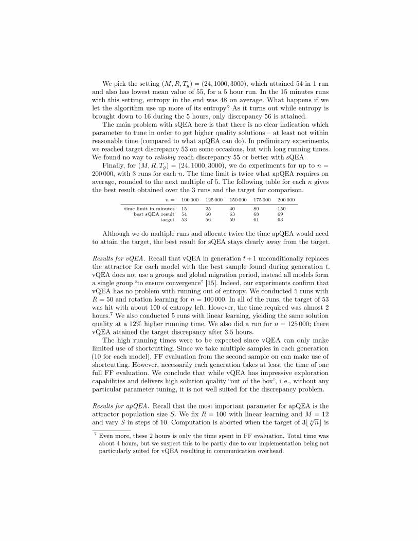
Finally, for pM,R, Tgq “ p24, 1000, 3000q, we do experiments for up to n “200 000, with 3 runs for each n. The time limit is twice what apQEA requires onaverage, rounded to the next multiple of 5. The following table for each n givesthe best result obtained over the 3 runs and the target for comparison.
n “ 100 000 125 000 150 000 175 000 200 000
time limit in minutes 15 25 40 80 150best sQEA result 54 60 63 68 69
target 53 56 59 61 63
Although we do multiple runs and allocate twice the time apQEA would needto attain the target, the best result for sQEA stays clearly away from the target.
Results for vQEA. Recall that vQEA in generation t` 1 unconditionally replacesthe attractor for each model with the best sample found during generation t.vQEA does not use a groups and global migration period, instead all models forma single group “to ensure convergence” [15]. Indeed, our experiments confirm thatvQEA has no problem with running out of entropy. We conducted 5 runs withR “ 50 and rotation learning for n “ 100 000. In all of the runs, the target of 53was hit with about 100 of entropy left. However, the time required was almost 2hours.7 We also conducted 5 runs with linear learning, yielding the same solutionquality at a 12% higher running time. We also did a run for n “ 125 000; therevQEA attained the target discrepancy after 3.5 hours.
The high running times were to be expected since vQEA can only makelimited use of shortcutting. Since we take multiple samples in each generation(10 for each model), FF evaluation from the second sample on can make use ofshortcutting. However, necessarily each generation takes at least the time of onefull FF evaluation. We conclude that while vQEA has impressive explorationcapabilities and delivers high solution quality “out of the box”, i. e., without anyparticular parameter tuning, it is not well suited for the discrepancy problem.
Results for apQEA. Recall that the most important parameter for apQEA is theattractor population size S. We fix R “ 100 with linear learning and M “ 12and vary S in steps of 10. Computation is aborted when the target of 3b 4
√nc is
7 Even more, these 2 hours is only the time spent in FF evaluation. Total time wasabout 4 hours, but we suspect this to be partly due to our implementation being notparticularly suited for vQEA resulting in communication overhead.

hit (a success) or a long flatline is observed (a failure), as explained in Sec. 2. Forselecting attractors, we use tournament selection: draw two solutions randomlyfrom P and use the better one with 60% probability and the inferior one with 40%probability (higher selection pressures appear to not help, this will be discussedin the full version). For each n and appropriate choices of S, we do 30 runs andrecord the following: whether it is a success or a failure, final discrepancy (equalstarget discrepancy for successes), running time (in minutes), mean final entropy.For failures, we also record the time at which the last discrepancy improvementtook place (for successes, this value is equal to the running time). The followingtable gives results grouped into successes and failures, all numbers are meanvalues over the 30 runs.
successes failuresn
1000 S # disc time entropy # disc time entropy last imp.
100 20 28 53σ“00 05σ“01 38σ“09 02 54σ“00 08σ“01 22σ“01 06σ“01
100 30 30 53σ“00 07σ“01 63σ“12 00 na na na na125 20 17 56σ“00 09σ“02 31σ“08 13 57σ“00 12σ“01 19σ“09 08σ“01
125 30 30 56σ“00 11σ“01 48σ“11 00 na na na na150 30 26 59σ“00 16σ“02 46σ“11 04 60σ“00 23σ“02 32σ“09 16σ“02
150 40 30 59σ“00 20σ“02 62σ“10 00 na na na na175 30 16 61σ“00 24σ“04 31σ“08 14 62σ“00 38σ“05 21σ“08 24σ“03
175 40 27 61σ“00 32σ“05 42σ“09 03 62σ“00 47σ“02 26σ“05 30σ“01
175 50 30 61σ“00 39σ“05 57σ“11 00 na na na na200 30 02 63σ“00 38σ“02 22σ“06 28 65σ“01 47σ“08 24σ“17 30σ“05
200 50 28 63σ“00 53σ“08 44σ“08 02 64σ“00 76σ“06 28σ“02 53σ“03
200 60 30 63σ“00 74σ“15 53σ“12 00 na na na na
We observe that by increasing S, we can guarantee the target to be hit.Dependence of S on n for freeness of failure appears to be approx. linear orslightly super-linear; ratios of S to n1000 for no failures are 0.30, 0.24, 0.27,0.29, and 0.30. But even if S is one step below the required size, discrepancyis only 1 away from the target (with an exception for n “ 125 000 and S “ 20,where we recorded discrepancy 58 in 1 of the 30 runs). Running times for failurestend to be longer than for successes, even if the failure is for a smaller S. This isbecause it takes some time to detect a failure by the flatline criterion. Larger Seffects larger entropy; failures tend to have lowest entropy, indicating that theproblem is the models having locked onto an inferior solution. The table alsoshows what happens if we do lazy S tuning, i. e., fixing S to the first successfulvalue S “ 30 and then increasing n: failure rate increases and solution quality forfailures deteriorates moderately. The largest difference to the target is observedfor n “ 200 000 and S “ 30, namely we got discrepancy 67 in 1 of the 30 runs;target is 63. For comparison, the best discrepancy we found via sQEA in 3 runsfor such n was 69 and the worst was 71. We conclude that a mistuned S doesnot necessarily have catastrophic implications, and apQEA can still beat sQEA.
Convergence. We plot (Fig. 1) discrepancy over time for 2 runs: the first hourof the 5-hour sQEA run with pM,R, Tgq “ p24, 1000, 3000q; and 1 for apQEAwith S “ 30, which is kept running after the target was hit (until the flatlinecriterion leads to termination). sQEA is shown with a dashed line and apQEA

0 10 20 30 40 50 60
5060
7080
90 sQEAapQEA
Time/Minutes
Dis
crep
ancy
Fig. 1: Discrepancy plotted over time for sQEA and apQEA
with a solid line. In the first minutes, sQEA brings discrepancy down faster, butis soon overtaken by apQEA (which reaches 51 in 10 minutes, target is 53).
Effect of Parallelization. We double number of cores from 96 to 192 and increasenumber of models to M “ 24, so that they can be treated in parallel with 8 coreseach. The following table shows results for 5 runs for each set of parameters. Firstconsider n “ 175 000 and 200 000. The best failure-free settings for S are 30 and50. In comparison with the best failure-free settings for 96 cores, time is reducedto 1739 “ 44% and 4274 “ 57%, respectively. 50% or less would mean a perfectscaling. When we do not adjust S, i. e., we use 50 and 60, time is reduced to2639 “ 67% and 5374 “ 72%, respectively. We also compute for n “ 250 000.
successes failuresn
1000 S # disc time entropy # disc time entropy last imp.
175 20 02 61σ“00 14σ“02 22σ“02 03 62σ“00 20σ“02 31σ“12 13σ“00
175 30 05 61σ“00 17σ“04 43σ“07 00 na na na na175 50 05 61σ“00 26σ“03 72σ“12 00 na na na na200 40 04 63σ“00 30σ“03 42σ“12 01 64σ“00 42σ“00 32σ“02 28σ“00
200 50 05 63σ“00 42σ“10 52σ“05 00 na na na na200 60 05 63σ“00 53σ“08 60σ“11 00 na na na na250 50 04 67σ“00 58σ“07 42σ“08 01 68σ“00 110σ“00 29σ“02 70σ“00
250 60 05 67σ“00 83σ“16 61σ“14 00 na na na na
5 Conclusion and Current Work
We have seen apQEA outperforming sQEA in terms of speed and solution qualityby a large margin on the discrepancy problem. For this problem, apQEA is easyto tune, since a single parameter, the size S of the attractor population, has aclear and foreseeable effect: it improves solution quality (if possible) at the priceof an acceptable increase in running time. vQEA has shown that it is possible toachieve the same solution quality as apQEA without parameter tuning, at theprice of an enormous running time and inter-process communication overhead. Itmay be possible to have the best of both worlds in one algorithm, i. e., to get ridof the S parameter in apQEA. Moreover we believe that it should be attemptedto mathematically analyze why vQEA and apQEA succeed where sQEA fails. We

also plan new applications of apQEA in the vast area of coloring of (hyper)graphsand other combinatorial problems. Concerning arithmetic progressions, we willinvestigate further ways to speed up the FF by exploiting combinatorial structures.
Acknowledgements. We thank the Deutsche Forschungsgemeinschaft (DFG)for Grants Sr7/12-3 (SPP “Algorithm Engineering”) and Sr7/14-1 (binationalworkshop). We thank Nikhil Bansal for interesting discussions.
References
1. Babu, G.S., Das, D.B., Patvardhan, C.: Solution of real-parameter optimizationproblems using novel quantum evolutionary algorithm with applications in powerdispatch. In: Proceedings of the IEEE Congress on Evolutionary Computation,Trondheim, Norway, May 2009 (CEC 2009). (2009) 1927–1920
2. Baluja, S.: Population-based incremental learning: A method for integrating geneticsearch based function optimization and competitive learning. Technical report,Carnegie Mellon University, Pittsburgh, PA (1994)
3. Bansal, N.: Constructive algorithms for discrepancy minimization. In: Proceedingsof the 51st Annual IEEE Symposium on Foundations of Computer Science, LasVegas, Nevada, USA, October 2010 (FOCS 2010). (2010) 3–10
4. Erdős, P., Spencer, J.: Probabilistic Methods in Combinatorics. Akadémia Kiadó,Budapest (1974)
5. Han, K.H., Kim, J.H.: Quantum-inspired evolutionary algorithm for a class ofcombinatorial optimization. IEEE Transactions on Evolutionary Computation 6(6)(2002) 580–593
6. Han, K.H., Kim, J.H.: On setting the parameters of quantum-inspired evolutionaryalgorithm for practical applications. In: Proceedings of the IEEE Congress onEvolutionary Computation, Canberra, Australia, December 2003 (CEC 2003). (2003)178–184
7. Harik, G.R., Lobo, F.G., Goldberg, D.E.: The compact genetic algorithm. Technicalreport, Urbana, IL: University of Illinois at Urbana-Champaign, Illinois GeneticAlgorithms Laboratory (1997)
8. Hauschild, M., Pelikan, M.: An introduction and survey of estimation of distributionalgorithms (2011)
9. Knieper, P.: The Discrepancy of Arithmetic Progressions. PhD thesis, Institut fürInformatik, Humboldt-Universität zu Berlin (1997)
10. Mani, A., Patvardhan, C.: An adaptive quantum inspired evolutionary algorithmwith two populations for engineering optimization problems. In: Proceedings of theInternational Conference on Applied Systems Research, Dayalbagh EducationalInstute, Agra, India, 2009 (NSC 2009). (2009)
11. Mani, A., Patvardhan, C.: A hybrid quantum evolutionary algorithm for solvingengineering optimization problems. International Journal of Hybrid IntelligentSystems 7 (2010) 225 – 235
12. Matoušek, J., Spencer, J.: Discrepancy in arithmetic progressions. Journal of theAmerican Mathematical Society 9 (1996) 195–204
13. Mühlenbein, H., Paaß, G.: From recombination of genes to the estimation of distri-butions I. binary parameters. In: Proceedings of the 4th International Conferenceon Parallel Problem Solving from Nature, Berlin, Germany, September 1996 (PPSN1996). (1996) 178–187

14. Patvardhan, C., Prakash, P., Srivastav, A.: A novel quantum-inspired evolutionaryalgorithm for the quadratic knapsack problem. In: Proceedings of the InternationalConference on Operations Research Applications In Engineering And Management,Tiruchirappalli, India, May 2009 (ICOREM 2009). (2009) 2061–2064
15. Platel, M.D., Schliebs, S., Kasabov, N.: A versatile quantum-inspired evolutionaryalgorithm. In: Proceedings of the IEEE Congress on Evolutionary Computation,Singapore, September 2007 (CEC 2007). (2007) 423–430
16. Roth, K.F.: Remark concerning integer sequences. Acta Arithmetica 9 (1964)257–260