A new paradigm and computational framework to …we asked subjects to press any sequence of their...

METHODSpublished: 14 July 2015

doi: 10.3389/fncom.2015.00087

Frontiers in Computational Neuroscience | www.frontiersin.org 1 July 2015 | Volume 9 | Article 87

Edited by:

Misha Tsodyks,

Weizmann Institute of Science, Israel

Reviewed by:

Maurizio Mattia,

Istituto Superiore di Sanità, Italy

Herve Rouault,

Janelia Research Campus, USA

*Correspondence:

Tobias Teichert,

Department of Psychiatry, University

of Pittsburgh, 200 Lothrop Street,

Pittsburgh, PA 15261, USA

[email protected]

Received: 28 January 2015

Accepted: 22 June 2015

Published: 14 July 2015

Citation:

Teichert T and Ferrera VP (2015) A

new paradigm and computational

framework to estimate stop-signal

reaction time distributions from the

inhibition of complex motor

sequences.

Front. Comput. Neurosci. 9:87.

doi: 10.3389/fncom.2015.00087

A new paradigm and computationalframework to estimate stop-signalreaction time distributions from theinhibition of complex motorsequencesTobias Teichert 1, 2* and Vincent P. Ferrera 1

1Department of Neuroscience, Columbia University, New York, NY, USA, 2Department of Psychiatry, University of Pittsburgh,

Pittsburgh, PA, USA

Inhibitory control is an important component of executive function that allows organisms

to abort emerging behavioral plans or ongoing actions on the fly as new sensory

information becomes available. Current models treat inhibitory control as a race between

a Go- and a Stop process that may be mediated by partially distinct neural substrates,

i.e., the direct and the hyper-direct pathway of the basal ganglia. The fact that finishing

times of the Stop process (Stop-Signal Reaction Time, SSRT) cannot be observed

directly has precluded a precise comparison of the functional properties that govern

the initiation (GoRT) and inhibition (SSRT) of a motor response. To solve this problem,

we modified an existing inhibitory paradigm and developed a non-parametric framework

to measure the trial-by-trial variability of SSRT. A series of simulations verified that the

non-parametric approach is on par with a parametric approach and yields accurate

estimates of the entire SSRT distribution from as few as ∼750 trials. Our results show

that in identical settings, the distribution of SSRT is very similar to the distribution of

GoRT albeit somewhat shorter, wider and significantly less right-skewed. The ability to

measure the precise shapes of SSRT distributions opens new avenues for research into

the functional properties of the hyper-direct pathway that is believed to mediate inhibitory

control.

Keywords: cognitive control, stop signal task, SSRT distribution, motor sequence, race model

Introduction

Inhibitory control is an important component of executive function that allows us to stopa planned or ongoing thought and action on the fly as new information becomes available(Logan, 1994; Williams et al., 1999; Boucher et al., 2007; Verbruggen and Logan, 2008). In theearly 80s, Logan and colleagues paved the way for a quantitative study of inhibitory controlby introducing the concept of an unobservable, inhibitory Stop process (Logan, 1981). In thestandard “countermanding” stop signal paradigm (Logan, 1981; Logan et al., 1984) subjectsare required to respond as quickly as possible to a Go signal, i.e., to press the right buttonin response to rightward arrow, or a left button-press for a leftward arrow. On a fraction ofthe trials, a Stop signal, presented at a random time after the Go signal, instructs subjects

http://www.frontiersin.org/Computational_Neuroscience

http://www.frontiersin.org/Computational_Neuroscience/editorialboard




http://dx.doi.org/10.3389/fncom.2015.00087


http://www.frontiersin.org

http://www.frontiersin.org/Computational_Neuroscience/archive

https://creativecommons.org/licenses/by/4.0/

mailto:[email protected]

http://dx.doi.org/10.3389/fncom.2015.00087

http://journal.frontiersin.org/article/10.3389/fncom.2015.00087/abstract

http://loop.frontiersin.org/people/20366/overview

http://loop.frontiersin.org/people/14935/overview

Teichert and Ferrera Non-parametric estimation of SSRT distributions

to withhold the response. Subjects are worse at inhibiting thepre-potent motor response as the Stop signal is presented closerin time to movement initiation. The horse-race model originallyformulated by Logan and Cowan conceptualizes the ability toinhibit the response as a race between a Go- and a Stop processthat are triggered by the presentation of the Go and Stop-signal,respectively (Logan, 1981, 1982; Logan et al., 1984; Logan andCowan, 1984; Stuphorn et al., 2000; Band et al., 2003; Verbruggenand Logan, 2008). If the Go process finishes first, the response willbe executed. If the Stop process finishes first, the response will beinhibited.

The success of the model depends on its ability to estimate theduration of the Go and Stop process. The Stop-signal reactiontime (SSRT) refers to the duration of the stop-process, i.e.,the time at which the Stop-process terminates relative to thepresentation of the Stop signal. This time is unobservable becauseno response is emitted on successfully inhibited Stop trials.Current mechanistic implementations of the horse-race modelsuch as the Hanes-Carpenter model (Hanes and Carpenter,1999), the independent race model (Boucher et al., 2007; Schalland Boucher, 2007) or the special race model (Logan et al.,2014) conceptualize the Stop process as a linear or noisyrise to threshold very similar to models that have successfullybeen used to model the finishing time of the Go process,i.e., GoRT. Other models of inhibitory control such as theinteractive race model (Boucher et al., 2007) provide morerealistic neural implementations, and allow the Go process andthe Stop process to interact. However, for the purposes of thecurrent manuscript, we make the same simplifying assumptionsof independence that underlie the original horse-race model(Logan, 1981).

In contrast to the finishing times of the Go process, thefinishing times of the Stop process cannot be observed directlyand need to be inferred through the absence of a response.Based on the assumption of independence between the Go andStop-process, the horse-race model enables the estimation ofthe mean and variance of the SSRT distribution, independentof its precise shape (Logan and Cowan, 1984). So far, however,it has been very challenging to estimate the precise shape ofthe SSRT distribution. This constitutes a significant limitationbecause SSRT distributions may provide important insight intounderlying mechanisms of inhibitory control in the same wayas RT distributions have been used to infer and restrict neuralmechanisms of decision-making. In particular, precise estimatesof SSRT distributions might distinguish subtle functionaldifferences between response initiation and response inhibitionthat are thought to be mediated by distinct neural substrates, i.e.,the direct and hyper-direct cortico-striatal pathway (Aron andPoldrack, 2006; Aron et al., 2007).

In 1990, two labs presented a theoretical method to deriveSSRT distributions from empirical hazard functions of observedGoRT on failed inhibition trials (Colonius, 1990; de Jong et al.,1990). However, hazard functions are notoriously noisy (Luce,1986) and the required number of stop-signal trials per stopsignal delay was estimated at a prohibitively large value of 250,000(Matzke et al., 2013). More recent approaches have circumventedthis problem by parametrizing the SSRT distribution (Colonius

et al., 2001; Matzke et al., 2013; Logan et al., 2014). This reducesthe number of trials that are needed to estimate the distribution,albeit at the cost of restricting the possible shapes that can berecovered.

Here we present an alternative approach to this problemby using a different type of inhibitory task that conveys moreinformation about SSRT on each trial. We based our task onthe complex movement inhibition task by Logan (1982). Inhis task professional typists were asked to type a word or asentence until a stop-signal instructed them to stop typing.Interestingly, Logan concluded that subjects were equally likelyto stop the complex motor sequence at any point in time duringthe word or sentence and that SSRT was independent of whetheror not the stop-signal appeared before or after typing began.This suggests that such typing tasks measure the same conceptof stop-signal reaction time measured in the countermandingtask. However, in contrast to the countermanding task, thecomplex movement inhibition task has the potential to providemore information about the occurrence of the stop-signal ona trial-by-trial basis. In particular, it provides a hard lowerestimate (the stop process must have finished after last keywas typed), and it provides a soft upper estimate (the stop-process must have finished before the next key press wouldusually have occurred). If the interval between key-presses isshort and predictable, each trial can provide a rather narrowwindow for SSRT. However, even for the skilled typists in Logan’sstudy, the interval between key-presses was on average 200msthus leaving a relatively large window that does not providea substantial increase in the amount of information per trial.Based on these considerations we modified Logan’s complexmovement inhibition task. To increase the rate of button presseswe asked subjects to press any sequence of their choosing onthe keyboard as fast as possible. Using this instruction evensubjects without special training in typing achieved mean inter-button press interevals around 30ms. This value is small enoughto provide a substantial increase in information that can begained on each trial. We refer to this task as the Motor-SequenceInhibition task (SeqIn).

The current study focuses the novel theoretical frameworkand analysis technique that we developed to extract informationabout the speed of inhibitory control from the SeqIn taskor similar tasks that require subjects to stop an ongoingmotor sequence with discrete behavioral output such as typing.In particular, the study highlights the feasibility of a noveldeconvolution method to extract non-parametric estimates ofentire SSRT distributions. The study also provides a detaileddescription of the subjects’ behavior in the SeqIn task tounderstand and rule out potential confounds.

Methods

Ethics StatementAll participants provided written signed informed consentafter explanation of study procedures. Experiments and studyprotocol were approved by the Institutional Review Boardsof Columbia University and New York State PsychiatricInstitute.






SeqIn TaskWe developed a novel SSRT task to facilitate the parameter-freeestimation of SSRT distributions with a reasonable number oftrials. In this new task subjects perform an unconstrained, self-ordered motor sequence (button-pressing on a keyboard at a rateof ∼30 per second) until a stop-signal instructs them to stop.The task is referred to as the Motor-Sequence Inhibition task(SeqIn). The time of the last button press relative to the stop-signal can be measured on each trial. Under the assumptionof independence of the Go and Stop process, the distributionof the observed last button presses can be understood as theconvolution of the distribution of SSRT with a distribution X thatcan be estimated from the data (see below). In the classical stop-signal or countermanding task, a single go and stop process raceagainst each other. Here, the task can be thought of as a sequenceof go processes (one for each key press) terminated by a singlestop process.

Behavioral TaskIn the SeqIn task subjects placed the fingers of their left andright hands on a keyboard as they would for typing. Eachfinger was assigned one particular key (left pinky: “a”; left ringfinger: “s”; left middle finger: “d”; left index finger: “f”; rightindex finger “j,” right middle finger: “k,” right ring finger: “l,”right pinky: “;”). A pure tone auditory cue (880Hz) instructedthe subject to immediately start pressing as many buttons aspossible using any sequence of finger-movements. Subjects werediscouraged from pressing multiple buttons at the same time,or holding down a button for a prolonged period of time.Otherwise, subjects were free to use any sequence of theirchoosing. In the current study we did not record the identityof the button presses. Hence, we cannot quantify the type ofsequences the subjects chose. However, from observation andown experience, the subjects chose regular repeating patterns offinger-movements. After a random interval (see below) duringwhich the subjects continued pressing buttons, the same auditorycue instructed them to stop as fast as possible. Hence, thesame stimulus served as the “go-signal” during transition to theresponse period as well as the “stop-signal” during transitionto the no-response period. An additional visual cue remindedsubjects of the current state of the task. This cue was greenduring the response period and red during the no-responseperiod.

A trial was defined as a single go-period followed by a singlestop-period. One run consisted of a series of 25 go and 25 stopperiods that were presented in immediate succession with notime between them (Figure 1A). The minimum duration of eachgo and stop period was 1.5 s. In addition to the 1.5 s baseline,we added a random interval that was drawn from a truncatedexponential distribution with a maximum value of 3.5 s and atime constant of 0.572 s. The total duration of each period variedbetween 1.5 and 5 s.

TrainingThe current study aimed to explore the possibilities of theSeqIn task in the best possible circumstances. Hence, particularcare was taken to recruit subjects that had already performed

other experiments and were known to be reliable psychophysicalsubjects. All subjects performed at least 3 runs of 25 trialsof the SeqIn task on a day prior to the start of the mainexperiment.

SetupThe experiments were performed on MacBook Pro Laptopcomputers. The task was programmed and executed withMatlab2009a using routines from Psychtoolbox-3 (Kleiner et al.,2007). Auditory go- and stop-signals were presented througha pair of commercial headphones (Bose) plugged into the3.5mm stereo jack. Experiments were conducted in a darkexperimental room. Viewing distance was 24 inches. The twoexperimental computers had 13 and 17-inch screens, giving riseto slightly different viewing angles. Individual subjects weretested consistently in one of the two setups. Screen resolution wasset to 1280 by 800 pixels.

SubjectsThe participants were 6 experienced human psychophysicssubjects (2 female) of age 22–42, including the first author. Allparticipants provided written informed consent after explanationof study procedures.

The Deconvolution AlgorithmThe horse-racemodel treats response inhibition as a race betweena Go- and a Stop process. If the Go process finishes first,the response is executed. If the Stop process finishes first,the response is successfully inhibited. We have expanded thisframework to include multiple Go processes to account for themultiple button presses in the SeqIn task. Figure 1B visualizesone particular mechanistic implementation of this expandedframework. It is based on the assumption that each go signaltriggers a Go process that activates a pattern generator. Thepattern generator sends out individual Go-processes that triggera response as soon as they reach a fixed threshold. The stop-signal triggers the initiation of a Stop process that inhibits theexecution of additional button presses as soon as it reachesthreshold. The considerations outlined below are non-parametricand independent of this particular implementation. If the lastbutton press was observed at time t, then the stop signal musthave finished at some unknown later point in time t+x. In thefollowing we will derive a method to estimate the distributionof x.

Let Ti i = 1, 2, 3, . . . be a series of random variables thatrepresent the time of the ith button press. By default we reportTi relative to the time of the stop signal (Figure 1C). However, theTi’s can also be reported relative to the time of the go signal. GoRTcan be defined as the time of the first button press T1 relative tothe go signal. Let N be an integer-valued random variable thatrepresents the number of the last executed button press beforethe Stop process finishes and prevents further responses. Hence,TN represents the time of the last button press. Let 1i be a setof random variables that describes the time between two adjacentbutton presses:

1i = Ti − Ti−1 ∀1 < i ≤ N (1)






FIGURE 1 | The motor-sequence inhibition paradigm (SeqIn). (A) In the

SeqIn paradigm subjects place all fingers of their left and right hand (except the

two thumbs) on a computer keyboard as they would for typing. During the

response period they are instructed to press as many buttons as possible

using whichever sequence of finger-movements they choose. Subjects are

discouraged from pressing multiple buttons at the same time, or holding down

a button for a prolonged period of time. After an exponentially distributed

waiting period, a 880Hz tone instructed them to start button pressing as

quickly as possible. After another exponentially distributed response period,

the same tone instructed subjects to stop the motor sequence as soon as

possible. The color of the fixation spot was green in the Go- and red in the

Stop-period. (B) One potential theoretical framework for the SeqIn paradigm:

the multi-process race model. Following the Go signal, a Go processes starts

developing toward a threshold that activates a pattern generator

thatgeneratessequencesofmotorcommands.A response isassumedtooccur

(Continued)






FIGURE 1 | Continued

whenever a motor command reaches the response threshold (Ti ). GoRT

was defined as the time of the first button press after the presentation of

the Go-signal (T1). The total number of observed button presses is

defined as N. Hence, the time of the last button press relative to the

Stop-Signal is TN. The Stop signal triggers the emergence of a Stop

process that also develops toward the response threshold. Once the

Stop process reaches the threshold at time S, all upcoming planned

button presses (N+ 1,N+ 2, . . . ) will be inhibited. The stop signal

reaction time can be determined as the sum of the last button press TNand an estimate of X, the difference between TN and S. The estimate of

X uses the distribution of observed button-press intervals to predict the

distribution of TN+1 (see Methods). (C) Example data set with times of

button presses aligned to the Go signal (left panel) and the Stop signal

(right panel). Each trial starts with the presentation of the go-signal, lasts

throughout the go-period as well as the subsequent stop-period. Trial

number was sorted according to the time of the first button press after

the Stop signal (orange points in right panel). (D) The distribution of last

button presses TN can be viewed as the convolution of the distribution of

X and the unobservable density of the Stop process S. Since the

distributions of X and TN can be either be directly measured or inferred

from the data, the SSRT distribution can be estimated via deconvolution.

For simplicity we assume that all 1i are independent and havethe same distribution:

F1i = F1 ∀i ∈ N (2)

Let S be a random variable that represents the time at whichthe Stop process finishes. Then X = S − TN represents thetime between the last button press and the termination of theStop process. Conversely, we can define S as the sum of TN

and X. Under the assumption that TN and X are independent,the distribution of S corresponds to the convolution of thedistributions of TN and X.

S = TN ∗ X (3)

Based on Equation (3) we can estimate the unobservabledistribution of S by deconvolving X from TN . The distributionof X can be estimated in two different ways. Both approaches arebased on the assumption that S and Ti are independent. The firstapproach is more intuitive and starts with the trivial observationthat X cannot be measured explicitly because S is not observable.However, based on the existing trial data we can simulate trials ina scenario where S is know. To that aim define a suitable variableS′ as the simulated time at which the stop-process terminates. Forthis simulated time-point S′ we can now pretend that all buttonpresses after S′ did not occur, as would have been the case if S′

had been the actual time at which the stop signal terminated. Inthe simplest case, we can define S′ = 0ms for all trials, i.e., pretendthat the stop-process terminates instantaneously at the exact timethe stop signal is presented. In analogy to our definition of Nas the number of the last button press before the termination ofthe actual stop-process, we can now define M as the number ofthe last button press before the termination of the simulated stopprocess. In this scenario it is possible to explicitly calculate X′ asthe difference between S′ and TM . As long as both S and S′ areindependent of Ti,the distribution of X′ will be identical to theunobservable distribution of X. Note that the definition of M isuseful only if S′ is smaller than S. Otherwise, we can’t be sure thatM was actually the last button press before S′: the terminationof the actual stop process at time S might have inhibited laterbutton presses that could have occurred before S′. In practice thisis an easy requirement to meet by only using S′ values before thepresentation of the stop signal, i.e., S’= 0. Of course it is similarlyimportant to chose S′ such that S′ > T1. To give subjects timeto establish a steady pressing routine, we use an even stricter

criterion and ensure that S′ is always at least 500ms larger thanT1. For each value of S′, we get one estimate of X′ for eachrecorded trial. Given the large number of trials recorded and thelarge range of possible values for S′ it is easy to estimate X′ andhence X with great precision.

The second approach is based on the density of inter-buttonpress intervals f1. To that aim we first assume that 1N+1 isknown and equal to a fixed value u. Due to the independence ofS and Ti, S is equally likely to have terminated at any point afterTN and before TN+u. Hence, X is uniformly distributed over theinterval from 0 to u, with a density equal to 1/u. This is true forany value of u. We can now integrate across all possible values uweighted by the likelihood that 1N+1 is equal to u:

FX (t) = P (X ≤ t)

=∫ ∞

0

(

min(t,u)u

)

f1du

=∫ t0 f1 (u) du+

∫ ∞

ttu f1du

= F1 (t) + t∫ ∞

t1u f1du

(4)

We can solve and differentiate Equation (4) numerically to obtainan estimate of the density of X. Due to the large number ofobserved inter-button press intervals, the distribution of X canbe estimated very accurately.

We confirmed that both methods yield numerically highlysimilar estimates of the distribution of X. The first approachprovides a simple intuition and can be interpreted as thedistribution of last button presses under the assumption of aninstantaneous stop signal. The second approach is appealingbecause of its more stringent mathematical derivation.

After estimating the density of X, we can use it to recover Sby deconvolving X from TN (Figure 1D). Convolutions cannotalways be inverted, in particular when the convolution kernel hasno power in a frequency band that the original signal does. Thiswas not a concern in the current case, as the convolution kernel Xhas a broad power spectrum (note the sharp edge in Figure 1D,left panel). To further stabilize the deconvolution process, thedistribution of TN was smoothed with a Gaussian kernel witha standard deviation of 16ms. This reduced the noise in theestimate of the distribution ofTN . In the noise-free case, the resultof the deconvolution should recover the SSRT density function Ssmoothed with the same 16ms Gaussian kernel. However, in thenoisy case, the result of the deconvolution needs to be processedfurther to ensure that the outcome fulfills the requirements of adensity function. In particular, the imaginary component of thedeconvolution was set to zero. We then integrated the resulting






raw density over time to recover a raw distribution function. Thelower time bound was defined as the latest time at which theraw distribution function was negative. Negative raw distributionvalues occurred due to small ripples of the raw density functionthat tended to be present at the left tail of the raw densityfunction. All density values below or equal to the lower boundtime were set to zero. Any residual negative density values abovethe lower bound time were also set to zero. Independent of theabove operations, density values below 90ms and above 550mswere set to zero. Finally, the resulting function was normalizedto a sum of one. Neither of these operations changed the overallshape of the distribution but were necessary in order to calculateexpected value, variance, and skew.

In addition to the model-free non-parametric deconvolutionalgorithm outlined above, it is also possible to use a parametricapproach. Here we convolved an exponentially modifiedGaussian distribution (ex-Gauss) with the distribution of X, andthen adjusted the parameters of the ex-Gauss such that the resultmatched the observed times of the last button press, TN . Similarlywe adjusted the parameters of the ex-Gauss to match the timeof the first button press, T1, or GoRT. In both cases, the fittingprocess used a maximum likelihood estimation technique. Toavoid infinite log-likelihood values during the fitting process weadded a lapse rate of 1% evenly spread over all time-bins. Theparametric approach has the advantage that it does not dependon the smoothing with the 16ms Gaussian kernel and hencerecovers the parameters of the actual SSRT andGoRT distributionrather than their smoothed version. This comes at the cost ofrestricting the possible range of shapes that can be recovered.

To verify the deconvolution approach, we used the samemethod to recover the known GoRT distribution (T1). Tothat aim, we first convolved the GoRT distribution with thedistribution of X. This was done empirically: for each trial nwe drew a random sample x(n) from the distribution of X. Thissample was subtracted from the GoRT of this trial:

CRT (n) = GoRT (n) − x (n)

CRT (Convolved Reaction Time) provides an estimate ofhow the RT distribution would look like if it could not bemeasured explicitly, but rather if it would have to be inferredin the same way as SSRT, i.e., by the absence of some otherdiscrete event. Most importantly, the distribution of CRT isan empirical convolution of GoRT and X. Hence, we canuse the deconvolution method to recover the original GoRTdistribution. This comparison provides a test for the accuracy ofthe deconvolution approach.

All computations were performed with the statisticalsoftware-package R (R Development Core Team, 2009).Densities were represented in 300 four-millisecond bins rangingfrom −400 to +800ms. Trials with extreme GoRT or TN valueswere excluded from the analysis. However, rejection criteria werevery liberal such that for 5330 trials in the seven data sets only15 trials were rejected. Trials were rejected if their GoRT wasbelow 90ms or if the time of the last button press TN happenedbefore the stop signal. The upper bounds for GoRT and TN

were defined as their median plus eight times the standard

deviation. The same criteria were used for the simulated datasets.

Analysis of Mean SSRT Independent ofDeconvolution ApproachIn addition to the deconvolution approach described above, itis possible to estimate the mean SSRT from the data using asimpler method that does not rely on the deconvolution method.This simpler method does not provide an estimate of the entiredistribution, but provides reliable estimates of mean SSRT fromas little as 75 trials. The method relies on the definition X =

S − TN , which can be reformulated to S = TN + X. Hence,E[S] = E[TN] + E[X]. We can estimate E[TN] as the meanof the observed TN , and E[X] from the distribution of X thatwas derived in Equation (4). The distribution of X depends onthe inter-button press intervals which remained rather constantthroughout the experiment. Hence, to a first approximationE[X] is a constant and E[S] is equal to the mean of TN plus aconstant.

Analysis of Recovered DensitiesThe deconvolution algorithm provides estimates of SSRT andGoRT density. To visualize the shape of the distributionsindependent of inter-subject differences in mean and variance wesubtracted out the mean and normalized the standard deviationto one. The normalization was performed on the labels of thetime-bins: Let t be the sequence of values that denotes thecenter of each density bin. We then re-assigned the labels foreach time bin by subtracting the mean and dividing by thestandard deviation: t′ = (t-E[t])/sqrt(V[t]). We then used linearinterpolation to estimate density values on a regular grid rangingfrom −8 to 8 standard deviations and a step size of 0.1. Theidentical approach was used to normalize the time-axes of thedistribution functions.

For visualization purposes we estimated the averagenormalized density over all subjects. To that aim we averagedthe individual normalized density functions for each bin acrossall subjects. This approach was aimed at extracting the shapeof the distribution while removing potential differences inmean and width. The normalized distribution functions wereaveraged using Vincent averaging. To that aim we picked asequence of probabilities ranging from 0.001 to 0.999 in stepsof 0.001. For each of these values we used linear interpolationto estimate the corresponding quantile. The mean of thesequantile values defined the average distribution function. Theresulting distribution function was defined on an irregular gridof time-values. We then used linear interpolation to estimate thedistribution function on the regular default grid described above(from -8 to 8 with a step size of 0.1).

The averaging process described above was aimed at removingdifferences in mean and standard deviation to highlight potentialdifferences in shape. We took another step to re-introducethe information regarding mean and standard deviation whilemaintaining the information about the shape of the distributions.To that aimwe first re-scaled the default time-axis with the squareroot of the mean of the individual variances. Then we then addedthe mean of the individual means to the rescaled time-axis. The






entire transformation allowed us to give a precise estimate of theaverage shape as well as their width and position.

Results

We developed a novel theoretical framework and analysistechnique to facilitate the parameter-free estimation of SSRTdistributions from the inhibition of an unconstrained motorsequence (button-pressing on a keyboard, see Figure 1 andMethods). Six subjects recorded one or more data sets of 525 ormore trials (mean 761 trials, maximum 1575 trials) of the SeqIntask. One subject recorded two data sets in two distinct settingsfor a total of 7 full data sets. Each trial corresponded to one go-and one stop-period and provided the times of all button pressesincluding the first button press after the go-signal, as well as thelast button press following the presentation of the stop-signal.

General Properties of Behavior in SeqIn TaskBefore moving on to the calculation of the entire SSRTdistribution, we describe some basic properties of the buttonpress patterns in the SeqIn task. In particular, we addressed threemain points: (1) What is the rate of button presses that thesubjects achieved? (2) Is there any evidence that the subjectsused stereotyped motor patterns? (3) Are parts of the sequenceballistic or can the motor sequence be interrupted with equalprobability at any point in time? (4) Are there any systematicchanges of SSRT or GoRT over time? All of these analyses areimportant to put the results of the following deconvolutionanalysis into perspective. The first and third points allow usto quantify the amount of information that can be gainedfrom a single SeqIn trial. The second point helps us gauge thecognitive effort involved in maintaining the motor sequences:it has been suggested that the generation of truly randomsequences may require significant cognitive effort. Hence, theuse of a stereotyped and presumably automated response patternsupports the idea that the subjects were free to focus on startingand stopping demands of the task without being distracted bythe task of maintaining the motor sequence. The fourth pointwill help us understand the potential contribution of systematicchanges in SSRT on the results of the deconvolution. Note thatfor these analyses we estimate mean SSRT using a more robustmethod that does not depend on the deconvolution approach (seeMethods).

Figure 2A shows the button press responses of the subjectsin a raster plot format either aligned to the Go (left panels) orStop signal (right panels). By sorting the order of the trials, itis possible to appreciate the cumulative distribution functionsof the times of the first and last button presses. Figure 2B plotsthe density of the inter-response intervals (IRI) averaged acrossall instances, and Figure 2C plots the mean IRI as a functionof button press number in each motor sequence. Subjectsachieved mean IRIs around 30ms corresponding to ∼34 buttonpresses per second. It is important to note that the high rateof button-presses is essential for our purposes to increase theinformation content of each trial. The shorter the average IRI,the more information each trial carries about the occurrence ofthe unobservable stop-process. If the last button press occurredat 200ms after the stop-signal, then the stop-process must have

finished some time between 200ms and the time at which thenext press would have occurred if it had not been inhibited.If subjects press a button on average once every 100ms, thisrestriction is less strict than if they press on average once every10ms. Hence, it was essential to allow subjects to use as manyresponse buttons as possible to increase the rate of button pressesand decrease the average IRI. We have also collected preliminarydata when subjects were only allowed to use a total of two or fourfingers. These preliminary studies revealed similar mean SSRTvalues, but required a larger number of trials.

The systematic variation of mean IRI with button pressnumber indicates that most subjects used stereotyped mini-sequences. We followed up on this assumption by calculating thecross-correlation of the mean IRIs for the first 40 button presses.If subjects use stereotyped mini-sequences, we would expectcyclic modulation of inter-button-response intervals. Given thata sequence would likely consist of all 8 fingers from both hands(subjects were not allowed to use their thumbs), we would expectthe inter-button press intervals to be auto-correlated with a lagof 8 button-presses. This is indeed what we observed in mostof the subjects (Figure 2D). We further tested if the stereotypedmini-sequences extend beyond the first couple of button presses.To that aim, we excluded the first 16 IRIs, expanded the analysisthroughout IRI number 80, and calculated IRI cross-correlationsafter subtracting out the mean IRI (Figure 2E). As expected,the cross-correlation values are significantly smaller due to theuse of single trial IRIs, rather than mean IRIs. Nevertheless, theanalysis indicates cyclic patterns for most of the subjects. Overall,our analysis suggests the use of a stereotyped and presumablyautomated response pattern. This indicates that the subjects werefree to focus on starting and stopping demands of the taskwithout being distracted by the task of maintaining the motorsequence.

The results depicted in Figure 2C show a systematic variationwhen IRIs are aligned to the last button press of each trial (righthand side of panels 2C). Given the existence of mini-sequencesoutlined above these variations likely arise because the stop-process is more or less likely to finish between different button-presses in the mini-sequence. For example, it might be possiblethat the motor sequence can only be stopped at the end of amini-sequence. This explanation would assume that the hazardrate for the stop-process changes at different times in the mini-sequence. If this were the case it would reduce the amount ifinformation gained from a single trial of the SeqIn task. However,there is an alternative explanation for the observed variationsthat is consistent with the idea that the stop-process is equallylikely to finish at any point in time during the mini-sequence:Figure 3 shows that we can observe almost identical variationswhen IRIs are aligned to the last button press prior to a randomevent that is by definition equally likely to occur at any pointduring the mini-sequence. In summary, the systematic variationsof IRI arise because the stop-process is more or less likely toterminate after a particular button press of the mini-sequence.However, this variation in likelihood is explained by the averagewait-time for the next button press in the mini-sequence, not avariation of the hazard rate at different points of the sequence(Figure 3C). Hence, the systematic variations of IRI in Figure 2Care not only consistent with, but the logical consequence of the






FIGURE 2 | Motor-sequence patterns the SeqIn task. (A) Left panel:

times of button presses (black dots) aligned to the go-signal. Each line

corresponds to one trial. Trials are sorted according to the time of the first

button press (orange dots). The green line corresponds to the mean GoRT.

Right panel: times of button presses aligned to the Stop Signal. Trials are

sorted according to the time of the last button press (orange dots). The red

line corresponds to the estimated mean SSRT that is calculated as the sum

of the mean of the last button press plus an estimate of the mean of X. (B)

Density of the inter-button-press intervals (IRI or 1i ). (C) Mean IRI as a

function of button press number in a trial, either relative to the first button

press (left side of panel) or the last button press in a trial (right side of panel).

(D) Cross correlation of the mean IRIs. Vertical lines are spaced at multiples

of 8, the number of fingers that subjects can use to generate the sequences.

The cross correlation includes the first 40 IRIs. (E) Mean of single-trial cross

correlation after subtracting the mean IRI that gives rise to the patterns in (D).

The data excludes the first 16 IRIs and extends up to IRI 80. Hence, these

cross-correlograms indicate rhythmic motor sequences that are not

phase-locked to response onset. The star refers to the fact that subject 1

contributed two data sets. The first data set is indicated as S1, the second

one is indicated as S1*.






FIGURE 3 | Modulation of IRIs prior to last button press. (A) Example of

systematic modulation of IRIs aligned to the last button press in each trial,

i.e., the last button press that could not be inhibited by the stop-process

(black). Almost identical modulations can be observed when IRIs are aligned

to the last button press prior to a random event, in this case the presentation

of the stop-signal (blue). (B) Same plot averaged across the population. (C)

Putative explanation of both phenomena: Subjects employ regular

“mini-sequences” consisting of either 4 or 8 button presses. Cartoon

example depicts a regularly repeating mini-sequence consisting of 4 button

presses executed with digits D1 trough D4 thus giving rise to IRIs 11 trough

14. The assumption is that the stop-process is equally likely to terminate at

any point during the sequence (gray polygon). The likelihood of the last IRI

being sampled e.g., from 11 is identical to the likelihood of the last button

press being D2. This in turn is proportional to the average time between D2

and D3, i.e., 12. Hence, the mix of 1i s that contribute to the last IRI prior to

a random event is not uniform, but proportional to 1(i+1)s. The star refers to

the fact that subject 1 contributed two data sets. The first data set is

indicated as S1, the second one is indicated as S1*.

fact that the stop-process is equally likely to finish at any pointin time of the ongoing mini-sequences. This result is consistentwith Logan’s finding in the complex movement inhibition taskthat typing can be aborted with equal probability at any point ina word or sentence.

The analysis in Figure 3 reveals another potentially interestingphenomenon: The biggest difference between the two IRIsequences occurs on the very last IRI. This finding suggeststhat the time of the last button press occurs ∼3ms laterthan expected. While this effect is small and does not reachsignificance after correcting for multiple comparisons, it maybe an indication that the stop-process is not an all-or-nothing process as suggested by the strict assumptions of theindependent race model. Rather, the finding would be more inline with the physiologically more realistic interactive race-model(Boucher et al., 2007).

We then tested if mean SSRT and mean GoRT changedsystematically over the course of the experiment. To that aimwe divided the data from each subject into 10 equally sizedbins (deciles) and calculated mean GoRT and SSRT for eachbin (Figure 4A). GoRT did not significantly vary as a functionof decile. For SSRT, however, there was a significant effect.Follow-up analyses revealed that this effect depended on one

specific data set (data set 1 of subject 1). This data set canbe considered an outlier for technical reasons: instead of beingcollected in small sessions of three blocks divided over multipledays/experimental sessions, it was collected in two long sessions.Excluding this data set yields flat SSRT estimates independent oftime in the experiment.

We further tested if mean GoRT and mean SSRT remainstable over the course of each recording session. To that aim wecalculated GoRT and SSRT for the first, second and third blockof each recording day separately. Figure 4B shows a pronouncedand significant SSRT slowdown over the course of the threeblocks. In contrast, there is no such effect for GoRT. If at all, thereis a small, albeit non-significant, effect in the opposite direction.We also tested if we can identify a slow-down of SSRT evenwithinindividual blocks of 25 trials. To that aim we divided each blockinto 3 sub-sets of trials. Between the first and third sub-set oftrials, we observed a significant SSRT slowdown on the orderof 4ms (Figure 4C). It is noteworthy that we also observed asignificant within-block slowdown of GoRT. The slowdown ofGoRT is less pronounced, but not significantly different from theone we observed for SSRT.

After establishing the general properties of the button-presspatterns in the task, we then turned to the deconvolution






A B C

FIGURE 4 | Systematic changes of SSRT and GoRT over time. (A) For

each subject, the total number of trials over all recording sessions was

divided into 10 equally sized deciles. GoRT did not significantly vary as a

function decile. For SSRT there was a significant effect. However, this effect

was carried exclusively by one data set. This data set can be considered an

outlier for technical reasons: instead of being collected in small sessions of

three blocks divided over multiple days, it was collected in two long sessions.

Excluding this data set yields flat SSRT estimates independent of time in the

experiment. (B) On each recording day, subjects performed at least 3 blocks

of 25 trials each. Changes of SSRT and RT are plotted as a function of block

number in the recording session. For SSRT, we observe a significant

slowdown over the course of each day. In contrast, no such effect is

observed for GoRT. (C) Slow-down of SSRT (black) and GoRT (gray) as a

function of trial number within each block of 25 trials. For both variables there

is a significant slow-down over the course of a block. The slowdown seems

more pronounced for SSRT, but this difference is not significant.

algorithm to recover the entire SSRT distribution from the timesof the last button press (see Figure 1 and Methods). However, inorder to assure that the findings from the real data were valid,we first performed simulations where we used the deconvolutionapproach to recover a known SSRT distribution.

SSRT Deconvolution of Simulated DataA series of simulations was conducted to estimate the accuracyof the deconvolution algorithm to recover the true distributionof the SSRT. For each simulated trial, a GoRT as well as a SSRTwere drawn from ex-Gauss distributions with known parameters(see below). In addition, a series of values was drawn from thedistribution of inter-response intervals (see Figure 1) observedacross all subjects in the study. T1 was defined as GoRT and thesubsequent Ti were defined as the cumulative sum of T1 and therandomly drawn inter-response intervals. The duration of the go-period was arbitrarily set to 1200ms. TN was defined as the lastbutton press before the time-point defined by the sum of stopsignal and the simulated SSRT. A data set consisting of N suchsimulated trials (N = 100, 250, 500, 1000, 2500, 5000, 10000)was then analyzed following the same deconvolution routineused for the actual data. The SSRT values were drawn fromone of three different ex-Gauss distributions (SSRT1 = ex-Gauss[µ = 190, σ = 0.030, τ = 0.0] sec, SSRT2= ex-Gauss[µ =

0.168, σ = 0.020, τ = 0.022] sec, SSRT3 = ex-Gauss[µ =

0.212, σ = 0.020, τ = −0.022] sec). For negative values ofτ we subtracted the exponential component from the Gaussiancomponent rather than adding it. The values were chosen toyield two skewed and one non-skewed distribution of equal mean(190ms) and standard deviation (30ms). Hence any differencein the recovered distribution would be attributable the change inshape of the distribution rather than its position or width.

The simulations show that the deconvolution algorithmaccurately recovers the different shapes of the distributions, inthis case a left-, non- and right-skewed shape. The accuracy

was quantified in two ways. First, we extracted 95% confidenceintervals (mean ± 1.96∗standard deviation) of the estimatedmean, standard deviation and skew. Figure 5 shows theconfidence intervals as a function of trial number. Even for arelatively low number of ∼750 trials the confidence intervals arequite small (less than ±4ms for mean and standard deviation,less than±0.4 for skew).

Note that the confidence intervals of the parameters of thedeconvolved distributions are only a small fraction larger thanthe confidence intervals of the parameters of the simulatedsample. This indicates that a large fraction of the varianceis due to variability of the simulated sample around its trueparameters rather than errors introduced by the deconvolutionalgorithm. After subtracting the recovered parameters fromthose of the underlying simulated sample (rather than theones of the theoretical distribution) the confidence intervals areapproximately half as wide (Figure 6). This indicates that thedeconvolution algorithm accurately captures small deviations ofthe simulated sample from the theoretical distribution they aredrawn from.

We further quantified the accuracy of the deconvolutionalgorithm by comparing it to the accuracy of a parametricapproach based on the fit of an ex-Gauss distribution. Figure 7shows that the confidence intervals of the parametric approachare highly similar to the ones obtained with the non-parametricapproach. It is important to keep in mind that in this case theparametric approach should be particularly effective as it uses thesame parametrization that was used to generate simulated data,an advantage that is not necessarily true for real data.

Finally we compared the accuracy of the two approachesusing the maximum difference between the recovered and thesmoothed empirical distribution function (Kolmogorv-SmirnovStatistic, Figure 8). For 750 trials we expect average KS valuesof the deconvolution approach is ∼0.02 and on par with the KSvalues obtained with the parametric approach.






FIGURE 5 | Ninety five percent confidence intervals (mean ±

1.96×standard deviation) of recovered mean, standard deviation and

skew of SSRT as a function of numbers of simulated trials N (1000

simulated data sets per confidence interval). The gray bars indicate

mean, standard deviation and skew of the simulated SSRT distributions that

were then used to simulate times of last button presses TN. The original SSRT

distributions were then recovered from the distributions of simulated TN using

the deconvolution algorithm. The black bars indicate the 95% confidence

interval for the deconvolved parameters when SSRTs were drawn from a

non-skewed Gaussian distribution of mean 190ms and standard deviation of

30ms. The red and green bars indicate the corresponding 95% confidence

intervals when SSRTs were drawn from positively and negatively skewed

ex-Gauss distributions of identical mean and variance. Note that the

confidence intervals of the deconvolved distributions are only a small fraction

larger than the confidence intervals of the actual empricial distributions. The

deconvolution algorithm operates on smoothed TN distributions (temporal

filtering with a 16ms Gaussian kernel). Hence, the recovered distributions

reflect properties of the filtered SSRT distribution. Filtering has no effect on the

mean. However, it does affect the standard deviation and the skew. The effect

of filtering can easily be removed from the estimate of standard deviation (note

that the sd estimates of the deconvolved distributions converge to the true

value of 30ms). A similar approach can be taken to recover true skew, but this

operation depends on the assumption that the underlying distributions are

ex-Gaussian. To maintain a model-free approach, we did not use such a

correction here. As a result, both positive (and negative) skew values are

underestimated (see red line). It is important to note, however, that the

recovered skew values matche the true skew value of the ex-Gauss that has

been filtered with the same temporal kernel that was used in the deconvolution

approach.

SSRT-Deconvolution of Real DataTo verify the deconvolution approach on real data, weempirically convolved the known GoRT distribution with ourestimate of X (see Figure 1 and Methods) and used the samedeconvolution method to recover the known GoRT distribution(see Methods). Figure 9A shows the recovered normalizedGoRT density function (middle column) as well as the originalsmoothed and normalized GoRT density function (left column).

FIGURE 6 | Mean, std.dev. and skew of the simulated SSRTs varies

around the true parameters due to the finite size of the sample. Hence,

the confidence bars in Figure 5 reflect both, the error of the deconvolution

algorithm as well as the random sampling of the empirical distribution upon

which the deconvolution is based. Here we subtract the recovered parameters

of the deconvolved distributions from those of the underlying empirical

distribution. The confidence intervals are substantially smaller, indicating that

the deconvolution algorithm accurately recovers the variability of the empirical

distribution. This is further validated by correlation between the empirical and

recovered mean (ρGauss = 0.77, ρex−Gauss = 0.77), standard deviation

(ρGauss = 0.54, ρex−Gauss = 0.66) and skew (ρGauss = 0.37,

ρex−Gauss = 0.63). These correlations are non-trivial, because the true mean,

standard deviation and skew are constant within the conditions.

The results highlight to ability of the deconvolution methodto recover the original GoRT distribution. The recovered GoRTdensities are noisier, but their specific shape, including thecharacteristic rightward skew, was accurately recovered. Theskew of the recovered GoRT distribution is significantly largerthan zero (1.1 ± 0.6, t-test, p < 0.05) and very similar to theskew of smoothed GoRT distribution (1.2± 0.7).

Using the same approach we deconvolved TN to obtain anestimate of the SSRT density. Similar to the recovered GoRTdensities, the SSRT densities were significantly right-skewed(0.9 ± 0.7, t-test, p < 0.05). The rightward skew is visible in therecovered densities (Figure 9A) as well as the quantile-quantileplots (Figure 9B).

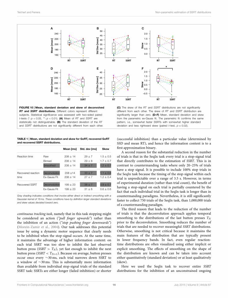
We then directly compared the first three moments of therecovered GoRT and SSRT distribution (Figures 10A–C andTable 1). Mean SSRT (199 ± 23) is 10ms shorter than meanGoRT (209 ± 15ms). This difference does not reach significance(paired t-test, df = 6, p = 0.36). Standard deviation of the SSRTdistribution (38 ± 7ms) is 5ms larger than standard deviationof the GoRT distribution (33 ± 7ms). This difference also doesnot reach significance (paired t-test, df = 6, p = 0.21). Meanskew for the SSRT distribution (0.9 ± 0.7) is ∼20% lower thanthe skew of the GoRT distribution (1.1 ± 0.6). This difference






FIGURE 7 | Comparison of the non-parametric deconvolution

algorithm with a paramtric approach based on ex-Gauss distributions.

Note that both approaches provide estimates of very similar accuracy. The

main advantage of the ex-Gauss approach is that is allows an unbiased

estimation of the skew—the deconvolution algorithm estimates the skew of

the smoothed function which is always deviated toward zero. The main

advantage of the deconvolution approach is that it does not restrict the range

of possible shapes of the distribution—in the current case the simulated

distributions were drawn from the same family of distributions that were used

in the parametric fit. For real data, the underlying distribution is not known and

may not be part of the ex-Gauss family.

does not reach significance (paired t-test, df = 6, p = 0.59).Similar results were found when using the parametric ex-Gaussapproach (Figures 10D–F and Table 1). In this case, however,the skew for the SSRT distributions was significantly smaller thanthe skew for the GoRTs (paired t-test, df = 6, p = 0.02). Wefollowed up on this discrepancy between the deconvolution andex-Gauss approach and noticed that the differencemanifests itselfin two subjects. The deconvolved SSRT densities of these subjectshave mass in a few long time-bins that could be consideredoutliers. In order to be maximally inclusive, the outlier rejectionfor the deconvolution approach was very liberal (see Methods).However, the parametric approach had implicitly classified thesebins as outliers thus yielding substantially smaller skew estimatesfor these two subjects. To exclude the impact of these potentialoutliers we used Bowley’s more robust quantile-based skewestimate. For a particular quantile 0 < u < 0.5, the Bowley’s skewestimate is defined as:

robustSkew (u) =F−1 (u) + F−1 (1− u) − 2F−1 (0.5)

F−1 (u) + F−1 (1− u)

Setting u to 0.1 yields Kelley’s absolute measure of skewness.Using Kelley’s quantile-based absolute measure of skewness, wefind a significantly smaller skew for the SSRT distributions

A

B C D

FIGURE 8 | The accuracy of the deconvolution algorithm measured as

the maximum difference between the smoothed empirical distribution

function and the deconvolved distribution (Kolmogorov-Smirnov

statistic). (A) As the number of simulated trials increases, the KS statistic

between the smoothed empirical distribution and the distribution recovered

with the deconvolution algorithm approaches zero. This is true regardless of

the skew of the distribution (red, black, and green color). The gray bars

indicate the same KS statistic for the distribution that was recovered by fitting

the ex-Gauss distribution. (B–D) Three examples for individual simulations with

representative KS-values for either 100, 250, and 750 trials. The black line

indicates the smoothed empirical distribution function, the red line the

recovered distribution. The examples were chosen to have a KS statistic of

0.05, 0.03, and 0.02, respectively. Note that for KS values of 0.03 and 0.02,

the recovered distribution is almost identical to the original distribution.

when using the deconvolution approach (paired t-test, df = 6,p = 0.04). This reconciles the findings of the parametric andthe non-parametric approaches and identifies smaller positiveskew as one of the main differences between GoRT and SSRTdistributions.

The overall picture conveyed by both methods is that ofstrikingly similar SSRT and GoRT distributions. However, ourresults suggest that SSRTs are somewhat shorter and have awider and less skewed shape. This finding is nicely illustratedin Figure 9C that directly compares position and shape of theaveraged SSRT andGoRT distributions side by side. Note that themain difference is the earlier rise of the ascending flank of theSSRT density function. In contrast, the falling flanks of the twodensity functions almost overlay.

Discussion

Response inhibition is a critical aspect of motor and cognitivecontrol, and is thought to involve prefrontal cortex and basalganglia; specifically, the hyperdirect cortico-striatal pathway.






A

B

C

FIGURE 9 | Comparing RT and SSRT distribution. Left column: RT

distributions smoothed with the same Gaussian kernel used for the

deconvolution algorithm. Middle column: RT distributions after empirical

convolution with X and subsequent application of the deconvolution

algorithm. Right column: deconvolved SSRT distributions. Comparison of left

and middle column visualize the modest distortions introduced by the

deconvolution algorithm. Comparison between middle and right column

visualize the difference between response initiation (RT ) and response

inhibition (SSRT ). (A) Normalized (z-transformed) empirical density functions

show significant rightward-skew (t-test, p < 0.05) for all three distributions

(smoothed RT, deconvolved RT and deconvolved SSRT ). (B)

Quantile-quantile plots visualize rightward skew as a concave curvature. (C)

Direct comparison of average GoRT and SSRT density function (left) and

distribution function (right). To account for different mean and standard

deviation, distributions were z-transformed, averaged and transformed back

using average values of mean and standard deviation for SSRT and GoRT,

respectively. The initial normalization allows effective averaging that maintains

the shape of the distributions despite considerable differences in mean and

standard deviation. The back-transformation reintroduces the differences in

mean and standard deviation that were lost in the initial normalization step.

Using a small sample of young healthy control subjects trainedon the task, the current study showcases the feasibility of thenon-parametric method to estimate entire SSRT distributionsfrom ongoing motor sequences with discrete behavioral outputsuch as typing. SSRT distributions allow us to study the fine-scale functional properties of the neural pathways that mediateinhibitory control with high temporal resolution. The non-parametric nature of the approach is particularly important andappealing as it complements a recently developed parametricapproach (Matzke et al., 2013). Previous non-parametricapproaches have never been implemented because they wereestimated to depend on a prohibitively large number of∼250,000stop signal trials per stop signal delay (SSD) for a total numberof ∼1,000,000 trials for each stop-signal delay to be used in theexperiment (Matzke et al., 2013). Our simulations show that

the current deconvolution approach yields adequate estimates ofentire SSRT distributions (KS statistic ∼0.02) for as little as 750trials.

This reduction in the number of required trials derives fromthe specific design of the SeqIn task. Rather than using a singlediscrete motor act, it uses a quasi-continuous motor sequence.Hence, our approach is related to an SSRT-paradigm developedby Morein-Zamir and colleagues (the continuous tracking task),where subjects continuously exert pressure with their index fingeruntil a stop signal instructs them to stop pressing (Morein-Zamir et al., 2004, 2006a,b). The continuous tracking task hasthe advantage that each trial provides one explicit estimateof SSRT and hence has a higher information content thana trial in the countermanding task. However, Morein-Zamirand colleagues also acknowledge one potential criticism of the






A B C

D E F

FIGURE 10 | Mean, standard deviation and skew of deconvolved

RT and SSRT distributions. Different colors represent different

subjects. Statistical significance was assessed with two-sided paired

t-tests (*: p < 0.05, **: p < 0.01). (A) Mean of RT and SSRT are

statistically not distinguishable. (B) The standard deviation of the RT

and SSRT distributions are not significantly different from each other.

(C) The skew of the RT and SSRT distributions are not significantly

different from each other. The skew of RT and SSRT distribution are

significantly larger than zero. (D–F) Mean, standard deviation and skew

from the parametric ex-Gauss fit. The parametric fit confirms the same

pattern, i.e., somewhat faster SSRTs with somewhat higher standard

deviation and less rightward skew (paired t-test, p = 0.02).

TABLE 1 | Mean, standard deviation and skew for GoRT, recovered GoRT

and recovered SSRT distributions.

Mean [ms] Std. dev [ms] Skew

Reaction time Raw 208 ± 14 29 ± 7 1.5 ± 0.5

Binned 208 ± 14 29 ± 8 1.7 ± 0.7

Smoothed 208 ± 14 34 ± 7 1.2 ± 0.7

Recovered reaction Deconvolution 208 ±14 33 ± 7 1.1 ± 0.6

time Ex-Gauss Fit 208 ± 14 27 ± 7 1.2 ± 0.4

Recovered SSRT Deconvolution 199 ± 23 38 ± 7 0.9 ± 0.7

Ex-Gauss Fit 199 ± 23 31 ± 6 0.6 ± 0.6

Gray shading indicates conditions that involve either direct or indirect smoothing with a

Gaussian kernel of 16ms. These conditions have by definition larger standard deviations

and skew values deviated toward zero.

continuous tracking task, namely that in this task stopping mightbe considered an action (“pull finger upwards”) rather thanthe inhibition of an action (“stop pushing finger downwards”)(Morein-Zamir et al., 2004). Our task addresses this potentialissue by using a dynamic motor sequence that clearly needsto be inhibited when the stop-signal occurs. At the same time,it maintains the advantage of higher information content: oneach trial SSRT was too slow to inhibit the last observedbutton press (SSRT > TN), yet fast enough to inhibit the nextbutton press (SSRT < TN+1). Because on average, button pressesoccur once every ∼30ms, each trial narrows down SSRT toa window of ∼30ms. This is substantially more informationthan available from individual stop-signal trials of the standardSSRT task: SSRTs are either longer (failed inhibition) or shorter

(successful inhibition) than a particular value (determined bySSD and mean RT), and hence the information content is to afirst approximation binary.

A second reason for the substantial reduction in the numberof trials is that in the SeqIn task every trial is a stop-signal trialthat directly contributes to the estimation of SSRT. This is incontrast to countermanding tasks where only 20–25% of trialshave a stop signal. It is possible to include 100% stop trials inthe SeqIn task because the timing of the stop-signal within eachtrial is unpredictable over a range of 3.5 s. However, in termsof experimental duration (rather than trial count), the benefit ofhaving a stop-signal on each trial is partially countered by thefact that each individual trial in the SeqIn task is longer than incountermanding paradigms. Nevertheless, it is still significantlyfaster to collect 750 trials of the SeqIn task, than 1,000,000 trialsof a countermanding paradigm.

The third reason that leads to the reduction of the numberof trials is that the deconvolution approach applies temporalsmoothing to the distributions of the last button presses TN

prior to the deconvolution. Smoothing reduces the number oftrials that are needed to recover meaningful SSRT distributions.Otherwise, smoothing is not critical because it maintains themain features of the distribution that are typically presentin lower frequency bands. In fact, even regular reaction-time distributions are often visualized using either implicit orexplicit smoothing. The effects of smoothing on the shape ofthe distribution are known and can be taken into accounteither quantitatively (standard deviation) or at least qualitatively(skew).

Here we used the SeqIn task to recover entire SSRTdistributions for the inhibition of an unconstrained ongoing






motor sequence (finger tapping). We also measured the GoRTdistributions for the initiation of the same motor sequence.We find that in the SeqIn task, mean GoRT and mean SSRTare statistically indistinguishable (GoRT: 208 ± 14ms; SSRT:199 ± 23ms). The finding of similar values for the two tasksmay seem somewhat surprising because in most other studiesmean RTs are 100–200ms slower than mean SSRTs. However,this apparent discrepancy is due to the fact that most otherparadigms measure choice RTs whereas the current paradigmmeasures “simple” RTs without a choice component. BecauseSSRT itself does not have a choice component, the currentapproach enables a fair comparison between GoRT and SSRT.Furthermore, the SeqIn task was specifically designed to facilitatethe comparison between GoRT and SSRT: the Go- and Stopsignals themselves are identical audio-visual events, and waitingtime distributions for the Stop- and Go signal are identical thusequalizing any anticipation/prediction for both signals. Afterthus equating the conditions for the two responses, mean latencyof response initiation is almost identical to the mean latency ofthe response inhibition. Note that we are not claiming statisticalequality of latency (or width). In fact, we expect that largersample size will reveal significantly shorter SSRT latencies. Wemerely point out that the absolute differences between the GoRTand SSRT distributions (significant or not) will be small relativetheir variability. This suggests largely similar (but not necessarilyidentical) functional properties of the two neural pathways thatmediate response inhibition and response initiation.

While both SSRT and GoRT have statisticallyindistinguishable mean latency and width in this small sample,SSRT distributions have significantly smaller skew. This isparticularly interesting, because it suggests that while GoRT andSSRT may be strikingly similar at first glance, there may be subtleyet meaningful differences. Once confirmed in a larger sample,these subtle differences can be used to test different mechanisticmodels of inhibitory control such as the independent race model(Boucher et al., 2007) or the Hanes-Carpenter model (Hanes andCarpenter, 1999) or the so-called special race model (Logan et al.,2014). The differences in the shape of SSRT could in principlebe mapped to parameters of these models, which in turn maymap onto parts of the direct and hyperdirect cortico-striatalpathways. Such a mechanistic and parametric approach willallow us to address a number of interesting questions: Are thedrift rates of the Go and Stop process identical? Are the heightsof the response- and the inhibition bound identical? Can thesame types of model that successfully explain GoRT distributionsprovide a satisfactory fit for SSRT? Can SSRTs be explainedin terms of a single mechanism, or do we need to considermore complex dual-process accounts? Some of these questionshave already begun to be explored in recent studies by Matzkeet al. (2013) and Logan et al. (2014). Because such approachesnecessarily depend on various parametrizations of the SSRTdistribution, it is particularly important to validate the shapeof parametrically recovered distributions with non-parametricmethods.

At this point we want to provide a brief comparison ofour non-parametrically recovered SSRT distributions with theparametrically recovered ones from the study of Matzke et al.

(2013). Overall, the mean SSRTs in our task (∼200ms) weresomewhat shorter than the ones found by Matzke and colleagues(∼220–230ms). This difference can most likely be attributedto our sample that was comprised of young, highly motivatedand experienced psychophysics subjects compared to a morerepresentative sample examined by Matzke and colleagues.However, it is important to note that the single-subject rangeof SSRTs in our sample is well within the range of SSRTsof Matzke’s and other SSRT studies. The shape of the SSRTdistribution in our study was narrower and less skewed. Toquantify this difference we compared our mean values of theparameters of the ex-Gaussian distributions in our study tothe ones estimated from Figure 17 in the paper by Matzke(mean of Gaussian component: 185 vs. ∼160ms; standarddeviation of Gaussian component: 23 vs. ∼20ms, and lastlythe exponential component: 20 vs. ∼60ms). Hence, the biggestdifference between the two studies is the exponential componentthat plays a much bigger role in the data by Matzke. It isimportant to note the large inter-individual variability of SSRTdistributions in the sample by Matzke. Some of the subjects havevery narrow and barely skewed SSRT distributions, very muchlike the subjects in our sample. Hence, it is possible that theoverall difference of SSRT distributions resembles the stricterselection criterion of subjects in our study. However, it is alsoimportant to note that Matzke observed a strong dependenceof SSRT distribution on the fraction of stop-signal trials. A dataset with 20% stop trials had significantly wider and more right-skewed distribution compared to a data set with 40% stop trials.While our paradigm is somewhat different it has a stop-signal in100% of the trials. Hence, some of the differences may also beattributed to the higher ratio of trials with a stop-signal.

Any estimate of SSRT or GoRT distributions implicitlyassumes that the variable in question is stationary duringthe data-acquisition period. Hence, we tested if there is anyindication of systematic changes in GoRT and SSRT overthe course of the experiment. Our data indicated that GoRTand SSRT stayed constant over the course of the experiment.This suggests that the subjects had enough training and wereperforming at ceiling levels during the entire experiment.However, we also tested whether performance stayed constantwithin each behavioral session consisting of 3 blocks of 25 trials.We observed a significant increase of SSRT over the courseof each behavioral session. GoRTs in contrast, remained stable.This systematic SSRT slow-down affects the comparison betweenGoRT and SSRT distributions that is based on all of the data,including blocks where SSRTs have already slowed down. Inparticular, it may have led to an overestimation of mean SSRTand the width of the SSRT distribution. In addition it may haveled to an underestimation of the skew of SSRT.

The SSRT slowdown was an incidental finding outside of themain focus of the study that was aimed at exploring technicalfeasibility of the deconvolution algorithm. It is not our intent todraw conclusions about SSRT slowdown form the small sampleof subjects. Nevertheless, the finding was intriguing enough towarrant some speculation about its potential origin. In particularwe want to rule out two trivial explanations. (1) The observedSSRT slowdown can not be explained by a reduction of attention






or arousal. If so, we would also expect a corresponding reductionof GoRT. (2) SSRT slowdown cannot be explained by a tradeoffin the balance between going and stopping: first, the minorreduction of GoRT does not seem to be consistent with thesubstantially larger increase of SSRT. Second, the SeqIn task isnot a dual task (as the countermanding task) where subjects needto prioritize either one or the other of the tasks.

We want to end the discussion by addressing certainlimitations and anticipating potential criticisms. (1) The analysisand interpretation of our data depends on the assumption ofindependence between the Go and Stop process. Our studydid not allow us to explicitly test this assumption. However,the assumption of independence is central not only to ourparadigm, but also to all other independent race-models. Studiesusing countermanding tasks have (a) indicated that violationsof independence are moderate, and (b) indicated that SSRTmeasured in countermanding tasks are reasonably robust againstviolations of the assumption of independence. Future studies willbe necessary to test if the same is true for the SeqIn task.

(2) The overwhelmingmajority of studies of inhibitory controluse the countermanding paradigm in which the to-be-inhibitedresponse is the result of a binary decision process. This type oftask has been extremely useful to study response inhibition inhealthy controls, and response inhibition deficits in a numberof neuro-psychiatric conditions. However, the concept of aStop process and SSRT, have been formulated independent ofthis particular paradigm. In fact, other paradigms have beendeveloped in the past, and were shown to correlate with SSRTmeasured in the countermanding paradigm. Hence, while termslike “SSRT” and “Stop process” have been intimately linked withthe countermanding paradigm, their use in the current context isverymuch within the original definition that does not specify thatthe to-be-inhibited action must be the result of a binary decisionprocess. Nevertheless, we want to caution that the SeqIn taskshould not be used as a substitute for established countermandingparadigms such as the Stop-It, SST or Vink task until it hasformally been shown to measure the same construct. However,based on the similarity of our task with the complex motion taskby Logan and the continuous tracking task by Morein-Zamirboth of which are believed to measure the same construct we areconfident that a validation study will confirm that the SeqIn taskmeasures the same construct.

(3) As pointed out above, it is not yet 100% clear if theSeqIn task measures the same variant of inhibitory control ascountermanding tasks. On the flipside of this argument, it is notclear if countermanding paradigms measure the same constructof inhibitory control that is involved in stopping ongoing motorsequences. Situations in which an ongoing motor sequence needsto be inhibited are prevalent in real life and constitute animportant area of study. For example, a quarterback may needto abort a particular play immediately after the snap, right beforethe ball leaves his hand, or at any point during the execution ofthe complex motor sequence that takes place between the snap

and the pass. In fact, even the standard example of inhibitorycontrol—a baseball player aborting a swing at a ball outsidethe strike-zone—arguably shares more similarity with the SeqInthan the countermanding task. Similarly, many situations ofinhibitory control of relevance in neuropsychiatric conditionsrequire the interruption of an ongoing motor sequence, suchas the interruption of perseverative hand washing in obsessivecompulsive disorder. In the most likely scenario, the two typesof inhibitory control involve identical neural mechanisms andinsight from one type of task will be relevant to both types ofscenario. However, it is also theoretically possible that differentneural mechanisms are involved in the two tasks and that insightsfrom standard SSRT tasks do not extrapolate to the inhibition ofongoing motor sequences. In this case the SeqIn task will be oneof only very few tasks to measure inhibitory control of ongoingmotor sequences.

(4) Based on the fact that SSRT and GoRT have similarmeans (∼200ms), it has been argued by some that the motorsequence in the SeqIn task may be stopped without the need toengage inhibitory control. Rather than inhibiting the ongoingmotor sequence it might be sufficient to just refrain fromissuing additional motor commands, or issue a new motorcommand (“pull all fingers upwards”) that will override othermotor commands and prevent additional finger taps. However,this assumption cannot account for the selective slow-downof SSRT across a session while RT remains stable. Also, it isimportant, albeit less obvious, to note that the same argumentcan be used to question the involvement of inhibitory controlin the countermanding task: While it may take on average400–600ms to press the correct button in the choice task,it will still take only ∼200ms to issue a simple “pull-all-fingers-upwards” motor command in response to the onset ofthe stop-signal. In fact, it has been argued that even in thecountermanding task an explicit stop process is not needed toexplain the behavioral findings (Salinas and Stanford, 2013).Hence, the selective SSRT slow-down in our task may be oneimportant piece of behavioral data that supports the presenceof an inhibitory process with distinct properties. In summary,these arguments clearly refute the idea that the duration ofthe GoRT relative to SSRT has any influence on whetheror not the stopping of the motor sequence needs to involveinhibitory control. However, we also want to acknowledgethat at this point, the SeqIn task has not been performed inthe context of fMRI or single-cell recordings. Hence, there iscurrently no neural evidence in favor or against the notion thatthe SeqIn task engages the hyper-direct pathway of the basalganglia.

Funding

This work was supported by National Institutes of Health GrantMH059244 (V.P.F.) and German Research Foundation GrantTE819/1-1 (T.T.).






References

Aron, A. R., Durston, S., Eagle, D. M., Logan, G. D., Stinear, C. M., andStuphorn, V. (2007). Converging evidence for a fronto-basal-ganglia networkfor inhibitory control of action and cognition. J. Neurosci. 27, 11860–11864.doi: 10.1523/JNEUROSCI.3644-07.2007

Aron, A. R., and Poldrack, R. A. (2006). Cortical and subcortical contributions toStop signal response inhibition: role of the subthalamic nucleus. J. Neurosci. 26,2424–2433. doi: 10.1523/JNEUROSCI.4682-05.2006

Band, G. P. H., van der Molen, M. W., and Logan, G. D. (2003). Horse-race modelsimulations of the stop-signal procedure. Acta Psychol. (Amst). 112, 105–142.doi: 10.1016/S0001-6918(02)00079-3

Boucher, L., Palmeri, T. J., Logan, G. D., and Schall, J. D. (2007). Inhibitory controlin mind and brain: an interactive race model of countermanding saccades.Psychol. Rev. 114, 376–397. doi: 10.1037/0033-295X.114.2.376

Colonius, H. (1990). A note on the stop-signal paradigm, or how toobserve the unobservable. Psychol. Rev. 97, 309–312. doi: 10.1037/0033-295X.97.2.309

Colonius, H., Özyurt, J., and Arndt, P. A. (2001). Countermanding saccades withauditory stop signals: testing the race model. Vision Res. 41, 1951–1968. doi:10.1016/S0042-6989(01)00084-0

de Jong, R., Coles, M. G., Logan, G. D., and Gratton, G. (1990). In search of thepoint of no return: the control of response processes. J. Exp. Psychol. Hum.

Percept. Perform. 16:164. doi: 10.1037/0096-1523.16.1.164Hanes, D. P., and Carpenter, R. H. (1999). Countermanding saccades in humans.

Vision Res. 39, 2777–2791.Kleiner, M., Brainard, D., and Pelli, D. (2007). What’s New in Psychtoolbox-3.

Available online at: www.psychtoolbox.orgLogan, G. D. (1981). “Attention, autmaticity and the ability to stop a speeded

choice response,” in Attention and Performance IX, eds J. B. Long and A.Baddeley (Hillsdale, NY: Erlenbaum), 205–222.

Logan, G. D. (1982). On the ability to inhibit complex movements: a stop-signalstudy of typewriting. J. Exp. Psychol. Hum. Percept. Perform. 8, 778–792. doi:10.1037/0096-1523.8.6.778

Logan, G. D. (1994). “On the ability to inhibit thought and action: a users’ guideto the stop signal paradigm,” in Inhibitory Processes in Attention, Memory, and

Language, eds D. Dagenbach and T. H. Carr (San Diego, CA: Academic Press),189–239.

Logan, G. D., and Cowan, W. B. (1984). On the ability to inhibit thoughtand action: a theory of an act of control. Psychol. Rev. 91, 295–327. doi:10.1037/0033-295X.91.3.295

Logan, G. D., Cowan,W. B., andDavis, K. A. (1984). On the ability to inhibit simpleand choice reaction time responses: a model and a method. J. Exp. Psychol.Hum. Percept. Perform. 10, 276–291.

Logan, G. D., Van Zandt, T., Verbruggen, F., and Wagenmakers, E.-J. (2014). Onthe ability to inhibit thought and action: general and special theories of an actof control. Psychol. Rev. 121, 66–95. doi: 10.1037/a0035230

Luce, R. D. (1986). “Representing response times as random variables,” in Response

Times, 8th Edn., eds D. Broadbent, J. McGaugh, N. Mackintosh, M. Posner, E.Tulving, and L. Weiskrantz (New York, NY: Oxford University Press), 1–46.

Matzke, D., Dolan, C. V., Logan, G. D., Brown, S. D., and Wagenmakers,E.-J. (2013). Bayesian parametric estimation of stop-signal reaction timedistributions. J. Exp. Psychol. Gen. 142, 1047–1073. doi: 10.1037/a0030543

Morein-Zamir, S., Chua, R., Franks, I., Nagelkerke, P., and Kingstone, A. (2006a).Measuring online volitional response control with a continuous tracking task.Behav. Res. Methods 38, 638–647. doi: 10.3758/BF03193896

Morein-Zamir, S., Nagelkerke, P., Chua, R., Franks, I., and Kingstone, A. (2004).Inhibiting prepared and ongoing responses: is there more than one kind ofstopping? Psychon. Bull. Rev. 11, 1034–1040. doi: 10.3758/BF03196733

Morein-Zamir, S., Nagelkerke, P., Chua, R., Franks, I., and Kingstone, A.(2006b). Compatibility effects in stopping and response initiation in acontinuous tracking task. Q. J. Exp. Psychol. (Hove). 59, 2148–2161. doi:10.1080/17470210500416375

R Development Core Team. (2009). R: A Language and Environment for Statistical

Computing. Vienna: R Foundation for Statistical ComputingSalinas, E., and Stanford, T. R. (2013). The countermanding task revisited:

fast stimulus detection is a key determinant of psychophysical performance.J. Neurosci. 33, 5668–5685. doi: 10.1523/JNEUROSCI.3977-12.2013

Schall, J. D., and Boucher, L. (2007). Executive control of gaze by the frontal lobes.Cogn. Affect Behav. Neurosci. 7, 396–412. doi: 10.3758/CABN.7.4.396

Stuphorn, V., Taylor, T., and Schall, J. D. (2000). Performance monitoring by thesupplementary eye field. Nature 408, 857–860. doi: 10.1038/35048576

Verbruggen, F., and Logan, G. D. (2008). Response inhibition in the stop-signalparadigm. Trends Cogn. Sci. 12, 418–424. doi: 10.1016/j.tics.2008.07.005

Williams, B. R., Ponesse, J. S., Schachar, R. J., Logan, G. D., and Tannock, R.(1999). Development of inhibitory control across the life span. Dev. Psychol.35, 205–213. doi: 10.1037/0012-1649.35.1.205

Conflict of Interest Statement: The authors declare that the research wasconducted in the absence of any commercial or financial relationships that couldbe construed as a potential conflict of interest.

Copyright © 2015 Teichert and Ferrera. This is an open-access article distributed

under the terms of the Creative Commons Attribution License (CC BY). The use,

distribution or reproduction in other forums is permitted, provided the original

author(s) or licensor are credited and that the original publication in this journal

is cited, in accordance with accepted academic practice. No use, distribution or

reproduction is permitted which does not comply with these terms.


www.psychtoolbox.org

http://creativecommons.org/licenses/by/4.0/








A new paradigm and computational framework to …we asked subjects to press any sequence of their...

Documents

Transcript of A new paradigm and computational framework to …we asked subjects to press any sequence of their...