A new indicator for the assessment of anthropogenic ...
205
Doctoral Thesis A new indicator for the assessment of anthropogenic substance flows to regional sinks. submitted in satisfaction of the requirements for the degree of Doctor of Science in Civil Engineering of the Vienna University of Technology, Faculty of Civil Engineering Dissertation Ein neuer Indikator zur Bewertung von anthropogenen Stoffflüssen in regionale Senken. ausgeführt zum Zwecke der Erlangung des akademischen Grades eines Doktors der technischen Wissenschaft eingereicht an der Technischen Universität Wien Fakultät für Bauingenieurwesen von Dipl.-Ing. Ulrich Kral Matrikelnummer 0225854 Lacknergasse 35/6, 1170 Wien Gutachter: o. Univ. Prof. Dr. Paul H. Brunner Institut für Wassergüte, Ressourcenmanagement und Abfallwirtschaft, Technischen Universität Wien, Karlsplatz 13/226, 1040 Wien, Österreich Gutachter: o. Univ. Prof. Dr. Stefanie Hellweg Institut für Umweltingenieurwissenschaften, Eidgenössische Technische Hochschule Zürich, Schafmattstraße 32, 8093 Zürich, Schweiz Wien, Juni 2014
Transcript of A new indicator for the assessment of anthropogenic ...

Doctoral Thesis
A new indicator for the assessment of anthropogenic substance flows to regional sinks.
submitted in satisfaction of the requirements for the degree of Doctor of Science in Civil Engineering
of the Vienna University of Technology, Faculty of Civil Engineering
Dissertation
Ein neuer Indikator zur Bewertung von anthropogenen Stoffflüssen in regionale Senken.
ausgeführt zum Zwecke der Erlangung des akademischen Grades eines Doktors der technischen Wissenschaft
eingereicht an der Technischen Universität Wien Fakultät für Bauingenieurwesen von
Dipl.-Ing. Ulrich Kral
Matrikelnummer 0225854 Lacknergasse 35/6, 1170 Wien
Gutachter: o. Univ. Prof. Dr. Paul H. Brunner
Institut für Wassergüte, Ressourcenmanagement und Abfallwirtschaft, Technischen Universität Wien, Karlsplatz 13/226, 1040 Wien, Österreich
Gutachter: o. Univ. Prof. Dr. Stefanie Hellweg
Institut für Umweltingenieurwissenschaften, Eidgenössische Technische Hochschule Zürich, Schafmattstraße 32, 8093 Zürich, Schweiz
Wien, Juni 2014


Abstract
Satisfying human needs requires an anthropogenic material turnover. After utilization, materials
either remain in the anthroposphere in terms of recycling products, or they leave the anthroposphere
in terms of waste and emission flows. The last two enter downstream sinks, man-made and natural
ones. The problem is that material flows to natural sinks may cause risks for human and
environmental health. To avoid overloading, several assessment frameworks have been put
forward. In an economy-wide perspective, a single score indicator focusing on substances that leave
the anthroposphere to regional sinks is missing. To overcome this gap, the thesis aims to develop a
new indicator and to compute the score for selected case studies.
To achieve these goals, four steps are needed. First, the indicator is defined as the environmentally
acceptable mass share of a substance in material flows that leave the anthroposphere to downstream
sinks. The resulting score ranges between 0% as worst case and 100% as best case. Second, a
methodology to determine the indicator components is presented, including (i) inventories based
on substance flow analysis, and (ii) impact assessment based on a distance-to-target approach.
Third, the framework developed is applied in three case studies including copper (Cu) and lead (Pb)
on an urban scale (City of Vienna) and Perfluorooctane Sulfonate (PFOS) on a national scale
(Switzerland). Fourth, recommendations are given for increasing the indicator score by means of
sink load reduction or enhancement of sink capacities.
The following results are obtained: In Vienna, 99% of Cu mass flows to regional sinks are
acceptable. However, the 0.7% of Cu entering urban soils and the 0.3% entering receiving waters
surpass acceptable levels. In the case of Pb, 92% of all mass flows to sinks prove to be acceptable,
and 8% are disposed of in local landfills with limited capacity. For PFOS, 96% of all flows to sinks
are acceptable. 4% cannot be evaluated due to a lack of quality criteria, despite posing a risk for
human health and the environment. The examples demonstrate the need for: (i) enhanced regional
landfill capacities or increased recycling rates, (ii) regional standards for assessing substance flows
to urban soils and receiving waters, (iii) appropriate data of good quality, and (iv) the extension of
the methodology to include exports to sinks in the hinterland.
The new indicator is of relevance for managing wastes and emissions because it identifies substance
flows to sinks that observe or neglect quality criteria, or that cannot be assessed due to missing
knowledge. Moreover, it serves for monitoring the performance of waste and environmental
management within a region, and for comparing the performance with other regions. For strategic
decisions such as design and evaluation of policies, the indicator allows an examination of the
effectiveness of directing substance flows to appropriate sinks. Finally, the indicator aggregates
complex information into an easy to understand score and is therefore highly instrumental for
communicating scientific research to decision makers and the public.
ii


Acknowledgements
I thank Paul H. Brunner for initiating and promoting the strategy concerning “clean material cycles
and final sinks”, for his supervision of this thesis and for his continuous support during the last four
years. My thanks goes also to Stefanie Hellweg for co-supervising the thesis.
I thank my scientific colleagues, with whom I collaborated on an international joint research project,
from which this thesis results. Katharina Kellner gathered so much data diligently and contributed
to a common research article. My thanks goes also to Hwong-Wen Ma, Pi-Cheng Chen, Chih-Yi
Lin, and Shi-Rong Chen from National Taiwan University for making the project possible, and for
their obligingness, kindness and efforts, which made the collaboration smooth and my visits in
Taiwan an unforgettable experience. I appreciate their endeavors in gathering data as well as their
generosity for contributing their broad scientific knowledge and for being available for discussion
in untold online-meetings.
I dedicate my special thanks and admiration to Claudia. She looked after our two sons Jakob and
Adrian with loving care while I was traveling to scientific conferences around the world to present
my research. Beyond that she is going to enrich our lives by giving birth to our third son, Lorin, in
the near future.
My gratitude also goes to Andrew Clarke. His painstaking proof-reading gave the textual quality
the necessary professional dimension. I am also indebted to at least ten anonymous researches for
reviewing the project proposal and the papers included in the thesis. I am grateful to Inge Hengl for
her support to improve the graphical quality of the figures, Claudia Klapproth and Maria Gunesch
for administrating the financial concerns and several trips to scientific conferences during the last
four years.
Finally, I acknowledge the funding by the Vienna University of Technology and the Austrian
Science Fund (FWF) for enabling scientific work to be carried out as a job without having to worry
about financial safeguarding.
iv

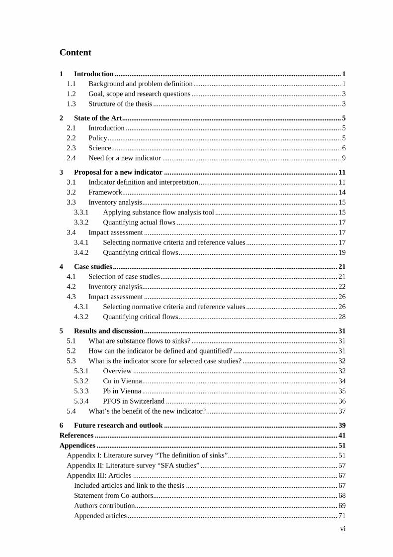
Content
1 Introduction ............................................................................................................................ 1 1.1 Background and problem definition ................................................................................. 1 1.2 Goal, scope and research questions .................................................................................. 3 1.3 Structure of the thesis ....................................................................................................... 3
2 State of the Art ........................................................................................................................ 5 2.1 Introduction ...................................................................................................................... 5 2.2 Policy ................................................................................................................................ 5 2.3 Science .............................................................................................................................. 6 2.4 Need for a new indicator .................................................................................................. 9
3 Proposal for a new indicator ............................................................................................... 11 3.1 Indicator definition and interpretation ............................................................................ 11 3.2 Framework ...................................................................................................................... 14 3.3 Inventory analysis ........................................................................................................... 15
3.3.1 Applying substance flow analysis tool ................................................................... 15 3.3.2 Quantifying actual flows ........................................................................................ 17
3.4 Impact assessment .......................................................................................................... 17 3.4.1 Selecting normative criteria and reference values .................................................. 17 3.4.2 Quantifying critical flows ....................................................................................... 19
4 Case studies ........................................................................................................................... 21 4.1 Selection of case studies ................................................................................................. 21 4.2 Inventory analysis ........................................................................................................... 22 4.3 Impact assessment .......................................................................................................... 26
4.3.1 Selecting normative criteria and reference values .................................................. 26 4.3.2 Quantifying critical flows ....................................................................................... 28
5 Results and discussion .......................................................................................................... 31 5.1 What are substance flows to sinks? ................................................................................ 31 5.2 How can the indicator be defined and quantified? ......................................................... 31 5.3 What is the indicator score for selected case studies? .................................................... 32
5.3.1 Overview ................................................................................................................ 32 5.3.2 Cu in Vienna ........................................................................................................... 34 5.3.3 Pb in Vienna ........................................................................................................... 35 5.3.4 PFOS in Switzerland .............................................................................................. 36
5.4 What’s the benefit of the new indicator? ........................................................................ 37
6 Future research and outlook ............................................................................................... 39 References ..................................................................................................................................... 41 Appendices .................................................................................................................................... 51
Appendix I: Literature survey “The definition of sinks” ............................................................ 51 Appendix II: Literature survey “SFA studies” ........................................................................... 57 Appendix III: Articles ................................................................................................................ 67
Included articles and link to the thesis ................................................................................... 67 Statement from Co-authors..................................................................................................... 68 Authors contribution ............................................................................................................... 69 Appended articles ................................................................................................................... 71
vi


Introduction
1 INTRODUCTION
1.1 Background and problem definition Satisfying human needs requires an anthropogenic material turnover. The turnover encompasses
material cycles and stocks that grow with the input of primary and secondary materials and that
decrease with the removal and loss of materials (Figure 1).
Figure 1: Anthropogenic material cycles are inevitably open, thereby including removals by the waste management system and dissipative losses from point and non-point emission sources (adopted from Stumm et al. 1974). Clean material cycles encompass materials without detrimental substances (black colored flows). Grey colored flows include substances that pose threats to human and environmental health.
Globally, the input of primary resources satisfies an increasing demand for materials (Dittrich et
al. 2013) and compensates for the (i) removal and (ii) loss of materials from anthropogenic material
cycles:
(i) The removal of materials has three key drivers: First, the limiting factors for recovering
valuable secondary resources, for instance, arise from waste collection schemes that might
not be oriented towards recycling, technologies that separate recyclable and non-recyclable
mass fractions, and economic conditions including the costs and benefits of secondary
material production (UNEP 2013). Second, to establish clean material cycles encompassing
secondary materials without impurities, hazardous substances contained in waste flows must
be removed by, before or during recycling (Brunner 2010, Kral et al. 2013). Despite
regulatory frameworks including the obligation to remove hazardous substances from waste
flows (e.g. Republik Österreich 2008, Republik Deutschland 2012), waste management
partly fails to fulfill this requirement. Examples are mineral oil in waste paper (ESFA 2012),
1

Introduction
brominated flame retardants in recycled plastic (Chen et al. 2009, Samsonek et al. 2013) and
recycled carcinogenic substances in construction waste (Rubli 2013, Deutscher
Bundesrechnungshof 2014). Third, strategies to minimize the environmental impacts of
material production contrast impacts from primary and secondary material production.
Therefore, the minimization of environmental impacts is rather based on optimal than on
high recycling rates. For copper, Stumm and Davis (1974) demonstrated that one ton has to
be composed of 60% secondary and 40% primary copper in order to require a minimum of
production energy. For treating cooling appliances, Laner et al. (2007) discussed the tradeoff
between environmental protection and resource conservation.
(ii) Material losses in terms of emissions occur throughout the entire process chain, including the
upstream, use, and downstream phases. Depending on the spatial release pattern, losses
originate from point or non-point sources. Hence, losses either result from the deliberate
intention to dissipate substances in the environment, such as with pesticides applied on land,
or might but cannot be avoided, such as with wear from brake pads (Lifset et al. 2012).
To conclude, materials leave the anthropogenic material cycle because the recovery rate of
secondary materials inevitably falls below 100% and because emissions occur along the life cycle
of materials. If materials leave the material cycle, sinks are required to accommodate these
materials.
The problem is that substance flows to natural sinks cause risks for human and environmental
health. To avoid burdens, natural sinks are available to a certain extent yet man-made sinks have to
be provided where natural sinks are lacking. Policy makers in the field of waste and environmental
management should consider to what extent the sinks can be loaded with substance flows and, if
needed, should provide suitable strategies to undershoot the limits. The effectiveness of directing
waste and emission flows to appropriate sinks is a measure of the environmental dimension of
sustainability.
2

Introduction
1.2 Goal, scope and research questions The thesis investigates the regional anthropogenic material turnover with respect to limits for the
discharge of substances to sinks. The goal is the development of an indicator that quantifies the
relative magnitude between acceptable and entire flows to regional sinks. The framework to
calculate the indicator score combines inventory analysis based on substance flow analysis and
impact assessment based on a distance-to-target weighting approach. Selected case studies
demonstrate both the applicability of the methodology and the benefits of the indicator score for
managing waste and emission flows.
The following research questions ensue from the goal of the thesis:
• What are substance flows to sinks?
• How can the indicator be defined and quantified?
• What is the indicator score for selected case studies?
• What’s the benefit of the new indicator?
The investigation into the regional metabolism focuses on substance flows (a) removed and lost
from the anthroposphere and entering regional sinks downstream, (b) discarded to natural and man-
made sinks, and (c) limited because of quality standards. Economic and social issues are excluded
from the assessment, despite their relevance for managing regional waste and emission flows.
1.3 Structure of the thesis The thesis is based on three research articles (see appendix III), which are framed from chapter 1
to chapter 6. Chapter 1 points to the need for sinks that accommodate substance flows, defines the
problem, goal, scope and research questions which are tackled in the thesis. Chapter 2 describes
state-of-the-art policy instruments and science-based indicators, and, finally, proposes a new
indicator for assessing mass flows to regional sinks. Chapter 3 defines the proposed indicator,
including the indicator components, and presents a framework to calculate the indicator score.
Chapter 4 presents the application of the indicator framework to three case studies for Copper and
Lead on a city level (Vienna) and PFOS on a national level (Switzerland). Chapter 5 presents the
results, thereby providing answers to the research questions. Chapter 6 gives an outlook for future
research.
The appendices include (I) background information regarding the definition of the term “sink”, (II)
the findings from a literature study regarding inventories based on substance flow analysis, and (III)
the articles as an integrative part of the thesis and puts them in the context of the thesis.
3

State of the Art
2 STATE OF THE ART This chapter (1) outlines the chapters’ framework, (2) describes policy instruments to manage waste
and emission flows, (3) presents science-based indicators and, finally, (4) highlights the need for a
new indicator.
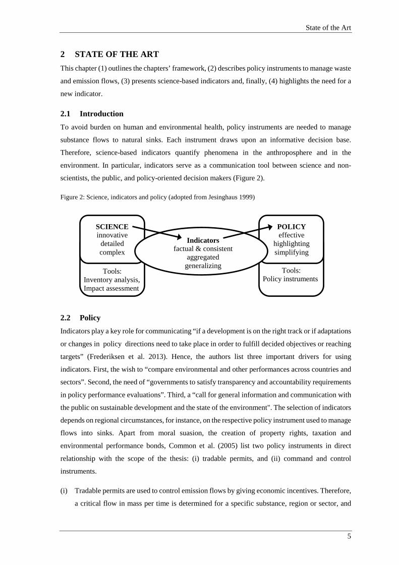
2.1 Introduction To avoid burden on human and environmental health, policy instruments are needed to manage
substance flows to natural sinks. Each instrument draws upon an informative decision base.
Therefore, science-based indicators quantify phenomena in the anthroposphere and in the
environment. In particular, indicators serve as a communication tool between science and non-
scientists, the public, and policy-oriented decision makers (Figure 2).
Figure 2: Science, indicators and policy (adopted from Jesinghaus 1999)
2.2 Policy Indicators play a key role for communicating “if a development is on the right track or if adaptations
or changes in policy directions need to take place in order to fulfill decided objectives or reaching
targets” (Frederiksen et al. 2013). Hence, the authors list three important drivers for using
indicators. First, the wish to “compare environmental and other performances across countries and
sectors”. Second, the need of “governments to satisfy transparency and accountability requirements
in policy performance evaluations”. Third, a “call for general information and communication with
the public on sustainable development and the state of the environment". The selection of indicators
depends on regional circumstances, for instance, on the respective policy instrument used to manage
flows into sinks. Apart from moral suasion, the creation of property rights, taxation and
environmental performance bonds, Common et al. (2005) list two policy instruments in direct
relationship with the scope of the thesis: (i) tradable permits, and (ii) command and control
instruments.
(i) Tradable permits are used to control emission flows by giving economic incentives. Therefore,
a critical flow in mass per time is determined for a specific substance, region or sector, and
Tools: Policy instruments
Tools: Inventory analysis, Impact assessment
SCIENCE innovative
detailed complex
POLICY effective
highlighting simplifying
Indicators factual & consistent
aggregated generalizing
5
State of the Art
period. With respect to the critical flow, tradable permits are issued by regulatory authorities
and a market-based mechanism allocates the permits to participating agents. For instance, the
Kyoto Protocol includes three options if a participating agent exceeds the allowed emissions
(United Nations 1998): (1) To buy permits from other participating agents. (2) To reduce
emissions in external regions that either participate or do not participate as agents. (3) To
enhance the removal of greenhouse gases by sinks on the basis of land use, land use change
and forestry.
(ii) Command and control instruments or “direct regulations” are widely used for managing
substance flows into sinks. Examples of direct regulations in Austria include quality standards
for surface waters (Republik Österreich 2006) and standards for waste disposal (Republik
Österreich 2008). Defining quality standards is a consensus-based process influenced, for
example, by scientific knowledge, available data, and technical and economic feasibility. The
points of command are identical with the points of control, supported by indicators along the
cause-effect chain of substances. For instance, pressure indicators include the level of
substance concentration in flows or annual flow rates. State indicators refer to the level of
substance concentration in environmental media. Damage indicators might refer to the
acceptable risk levels, despite the difficulty in defining them (Hunter et al. 2001).
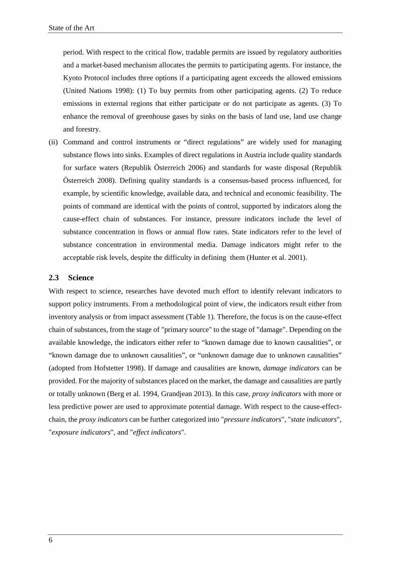
2.3 Science With respect to science, researches have devoted much effort to identify relevant indicators to
support policy instruments. From a methodological point of view, the indicators result either from
inventory analysis or from impact assessment (Table 1). Therefore, the focus is on the cause-effect
chain of substances, from the stage of "primary source" to the stage of "damage". Depending on the
available knowledge, the indicators either refer to “known damage due to known causalities”, or
“known damage due to unknown causalities”, or “unknown damage due to unknown causalities”
(adopted from Hofstetter 1998). If damage and causalities are known, damage indicators can be
provided. For the majority of substances placed on the market, the damage and causalities are partly
or totally unknown (Berg et al. 1994, Grandjean 2013). In this case, proxy indicators with more or
less predictive power are used to approximate potential damage. With respect to the cause-effect-
chain, the proxy indicators can be further categorized into "pressure indicators", "state indicators",
"exposure indicators", and "effect indicators".
6
State of the Art
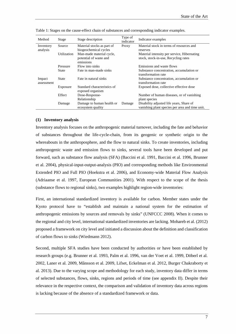
Table 1: Stages on the cause-effect chain of substances and corresponding indicator examples.
Method Stage Stage description Type of indicator Indicator examples
Inventory analysis
Source Material stocks as part of biogeochemical cycles
Proxy Material stock in terms of resources and reserves
Utilization Man-made material cycle, potential of waste and emissions
Material intensity per service, Hibernating stock, stock-in-use, Recycling rates
Pressure Flow into sinks Emissions and waste flows State Fate in man-made sinks Substance concentration, accumulation or
transformation rate Impact assessment
State Fate in natural sinks Substance concentration, accumulation or transformation rate
Exposure Standard characteristics of exposed organism
Exposed dose, collective effective dose
Effect Dose-Response-Relationship
Number of human diseases, or of vanishing plant species
Damage Damage to human health or ecosystem quality
Damage Disability adjusted life years, Share of vanishing plant species per area and time unit.
(1) Inventory analysis
Inventory analysis focuses on the anthropogenic material turnover, including the fate and behavior
of substances throughout the life-cycle-chain, from its geogenic or synthetic origin to the
whereabouts in the anthroposphere, and the flow to natural sinks. To create inventories, including
anthropogenic waste and emission flows to sinks, several tools have been developed and put
forward, such as substance flow analysis (SFA) (Baccini et al. 1991, Baccini et al. 1996, Brunner
et al. 2004), physical-input-output-analysis (PIO) and corresponding methods like Environmental
Extended PIO and Full PIO (Hoekstra et al. 2006), and Economy-wide Material Flow Analysis
(Adriaanse et al. 1997, European Communities 2001). With respect to the scope of the thesis
(substance flows to regional sinks), two examples highlight region-wide inventories:
First, an international standardized inventory is available for carbon. Member states under the
Kyoto protocol have to “establish and maintain a national system for the estimation of
anthropogenic emissions by sources and removals by sinks” (UNFCCC 2008). When it comes to
the regional and city level, international standardized inventories are lacking. Mohareb et al. (2012)
proposed a framework on city level and initiated a discussion about the definition and classification
of carbon flows to sinks (Wiedmann 2012).
Second, multiple SFA studies have been conducted by authorities or have been established by
research groups (e.g. Brunner et al. 1993, Palm et al. 1996, van der Voet et al. 1999, Döberl et al.
2002, Laner et al. 2009, Månsson et al. 2009, Lifset, Eckelman et al. 2012, Burger Chakraborty et
al. 2013). Due to the varying scope and methodology for each study, inventory data differ in terms
of selected substances, flows, sinks, regions and periods of time (see appendix II). Despite their
relevance in the respective context, the comparison and validation of inventory data across regions
is lacking because of the absence of a standardized framework or data.
7

State of the Art
(2) Impact assessment
Inventory data are of a descriptive nature. Because of their physical accounting unit “mass”, they
rely on the “equivalence of different emissions with unequal environmental impacts” (Jungbluth et
al. 2012). To assess the impacts, the substance flows have to be characterized, normalized and
weighted by normative methods (Brunner 2002). Therefore, inventory data are combined with
impact assessment methods such as Life Cycle Impact Assessment (e.g. Boesch et al. 2009,
Venkatesh et al. 2009, Rochat et al. 2013, Vadenbo et al. 2013, Boesch et al. 2014), Exposure and
Risk Assessment (e.g. Guinée et al. 1999, Gottschalk et al. 2010, Jang et al. 2012, Chen et al. 2013,
Lesmes-Fabian et al. 2013), cost-effective assessment in the field of waste management (Döberl,
Huber et al. 2002), and critical load concepts for specific flows into environmental media (Nagl
1996, Spranger et al. 2004). With respect to the cause-effect chain of substances, each method
provides indicators at a specific stage (Table 2).
Table 2: Impact assessment methods provide proxy and damage indicators.
Method Type of indicator Reference Proxy Damage
Material intensity per service X Ritthoff et al. (2002) Ecological Footprint X Wackernagel et al. (1996) Sustainable Process Index X Krotscheck et al. (1996) Entropy index X Rechberger et al. (2002), Sobańtka (2013) Ecological Scarcity 2006 Frischknecht et al. (2009) ReCiPe 2008 X Goedkoop et al. (2012) Risk assessment X McKone et al. (2002) Cost-Effective Method X Döberl, Huber et al. (2002) Critical load method X van het Bolcher et al. (2000), Hellweg et al. (2005)
The Material Intensity per Service aggregates the amount of materials along the life cycle chain of
products and services. Ecological Footprint and the Sustainable Process Index provide a single
indicator on an area base. The entropy index is used to quantify the dilution or concentration
performance of processes for elements and compounds. Life cycle impact methods provide
indicators related to impact categories with an option to aggregate them into a single score. For
example, Ecological Scarcity 2006 provides a pressure indicator in terms of a single score with
Eco-Points for each intervention. ReCiPe 2008 provides three damage indicators (damage to
resources, ecosystems, and human health) and weighting factors to aggregate the three indicators
into a single score. Risk assessment methods provide damage indicators of absolute risk in view of
human and environmental health. The cost-effective method is based on a distance-to-target
approach and yields a single score. Critical load concepts provide pressure indicators such as the
critical deposition on land, and the critical flow from landfills to subsurface layers.
8

State of the Art
2.4 Need for a new indicator According to chapter 1.1, the problem is that substance flows into natural sinks pose risks for human
and environmental health. To manage these risks, decision makers should consider to what extent
the sinks can be loaded with substance flows and, if needed, should provide suitable strategies to
undershoot the limits. Therefore, policy instruments encompass tradable permits and command and
control strategies (chapter 2.2), including relevant indicators (chapter 2.3). If substance flows to
regional sinks are managed, the evaluation of success depends on the policy instrument and
therefore on the number of managed flows:
• Tradable permits regulate a specific substance flow to a specific sink. The success control
can be monitored by a simple indicator: The relative magnitude of accepted and entire flows
to the sink:
Indicator score = Accepted flow to sink
Entire flow to sink∗ 100
For example, the greenhouse gas emissions in the Austrian economy are reported on an
annual base, and the reduction target has been agreed on under the Kyoto Protocol at minus
13% compared to the emissions in the year 1990 (Anderl et al. 2013). Based on this
information, Figure 3 plots the indicator score for greenhouse gas emissions in Austria from
1990 – 2011. As long as the score stays below 100%, adjustments need to be made or
measures need to be taken in order to reach the emission target. Based on Figure 3, it is
obvious that the Austrian economy emitted more than has been allowed. To conclude,
tradable permits from external regions have to be allocated to the Austrian economy.
Figure 3: Indicator score for greenhouse gases (CO2-equivalents) in the Austrian economy, from the year 1990 to 2011.
Up to now, tradable permits have been available for less than 10 substances and for selected
regions only (Common and Stagl 2005). For most substances and regions, cross-regional
assessment and management of substance flows with tradable permits is lacking. This lack
therefore amounts to the absence of an easily understandable indicator for most substances.
0%
20%
40%
60%
80%
100%
1990
1991
1992
1993
1994
1995
1996
1997
1998
1999
2000
2001
2002
2003
2004
2005
2006
2007
2008
2009
2010
2011
Indi
cato
r sco
re [%
]
9

State of the Art
• In contrast to tradable permits, command and control instruments evaluate a specific
substance in several flows to multiple sinks by various indicators. For instance, carbon to air
has to meet an international agreed emission standard, whereas carbon to landfills has to meet
national standards. Consequently, success control in view of reaching targets is based on flow
by flow assessment. To provide overall region-wide information about the disposal of
substances in sinks, Döberl et al. (2004) proposed a new indicator for monitoring the
environmental dimension of sustainability:
Indicator score = Amount of substances a region or process directs in appropiate final sinks
Total amount of substances emitted by a region or process
Apart from the proposed indicator definition, a framework for calculating the indicator
components has not been presented.
To conclude, with respect to policy instruments and relevant indicators today, the focus is rather on
single flows than on entire flows to sinks. An overall assessment of substances is lacking since
substances that have been removed or lost from the anthroposphere to regional sinks are not
evaluated by a common framework today. To overcome the gap in favor of a substance-oriented
policy, a new indicator is needed. Consequently, the thesis proposes a new indicator for quantifying
the relative magnitude of acceptable and entire flows to regional sinks. The regional assessment of
flows is (a) needed to manage material stocks and flows within the region itself, and is (b) required
to identify the need for sinks in external regions and to develop suitable strategies to monitor and
control external sink loads.
10

Proposal for a new indicator
3 PROPOSAL FOR A NEW INDICATOR This chapter proposes a new indicator, including (1) its definition and interpretation, and (2) the
framework to calculate the indicator score.
3.1 Indicator definition and interpretation A new indicator is proposed for assessing substance flows to regional sinks caused by the removal
and loss of substances from the anthroposphere. With respect to a specific substance, region and
period, the indicator λ quantifies “the acceptable mass share in flows to regional sinks”. Therefore,
it determines the relative magnitude between acceptable and entire sink loads:
λ = Acceptable sink load
Entire sink load∗ 100 Equation 1
Both the acceptable and entire sink loads are given in mass per time. Consequently, the indicator
score is dimensionless, ranging from 0% to 100% (Figure 4). Achieving 100% means that the total
mass of a substance within sink loads is acceptable. Less than 100% means that there is a certain
mass fraction within sink loads that overshoot accepted quality standards. Consequently, the
increase of the indicator score up to 100% is seen as good and worth striving for.
Figure 4: The entire sink load represents 100%, whereas the indicator score λ is equal to the acceptable mass share in flows to regional sinks and the complementary amount (100% minus λ) is equal to the unacceptable mass share in flows to regional sinks.
0%
100%
Unacceptable mass share in flows to regional sinksAcceptable mass share in flows to regional sinks
λ
11

Proposal for a new indicator
To operationalize the qualitative indicator definition from Equation 1, the following definitions are
given:
λ = ∑𝐹𝐹𝑎𝑎,𝑖𝑖
𝑅𝑅𝑅𝑅𝑅𝑅𝑖𝑖𝑅𝑅𝑅𝑅
∑𝐹𝐹𝑖𝑖𝑅𝑅𝑅𝑅𝑅𝑅𝑖𝑖𝑅𝑅𝑅𝑅 ∗ 100
Equation 2
𝐹𝐹𝑎𝑎,𝑖𝑖𝑅𝑅𝑅𝑅𝑅𝑅𝑖𝑖𝑅𝑅𝑅𝑅 = �
𝐹𝐹𝑐𝑐,𝑖𝑖𝑅𝑅𝑅𝑅𝑅𝑅𝑖𝑖𝑅𝑅𝑅𝑅
F𝑖𝑖𝑅𝑅𝑅𝑅𝑅𝑅𝑖𝑖𝑅𝑅𝑅𝑅
forfor ∝
𝑅𝑅𝑅𝑅𝑅𝑅𝑖𝑖𝑅𝑅𝑅𝑅≥ 0∝𝑅𝑅𝑅𝑅𝑅𝑅𝑖𝑖𝑅𝑅𝑅𝑅< 0
with Equation 3
𝛼𝛼𝑖𝑖𝑅𝑅𝑅𝑅𝑅𝑅𝑖𝑖𝑅𝑅𝑅𝑅 = 𝐹𝐹𝑖𝑖
𝑅𝑅𝑅𝑅𝑅𝑅𝑖𝑖𝑅𝑅𝑅𝑅 − 𝐹𝐹𝑐𝑐,𝑖𝑖𝑅𝑅𝑅𝑅𝑅𝑅𝑖𝑖𝑅𝑅𝑅𝑅 Equation 4
𝐹𝐹𝑖𝑖𝑅𝑅𝑅𝑅𝑅𝑅𝑖𝑖𝑅𝑅𝑅𝑅 = �βi0
forfor βi > 0
βi ≤ 0 with Equation 5
βi = min,i − mout,i Equation 6
where the index 𝑖𝑖 stands for a process 𝑖𝑖, ∑𝐹𝐹𝑎𝑎,𝑖𝑖𝑅𝑅𝑅𝑅𝑅𝑅𝑖𝑖𝑅𝑅𝑅𝑅 is the acceptable sink load, ∑𝐹𝐹𝑖𝑖
𝑅𝑅𝑅𝑅𝑅𝑅𝑖𝑖𝑅𝑅𝑅𝑅 is the
entire sink load. 𝐹𝐹𝑎𝑎,𝑖𝑖𝑅𝑅𝑅𝑅𝑅𝑅𝑖𝑖𝑅𝑅𝑅𝑅 is an acceptable flow in a region, 𝐹𝐹𝑖𝑖
𝑅𝑅𝑅𝑅𝑅𝑅𝑖𝑖𝑅𝑅𝑅𝑅 is an actual flow in a region,
𝐹𝐹𝑐𝑐,𝑖𝑖𝑅𝑅𝑅𝑅𝑅𝑅𝑖𝑖𝑅𝑅𝑅𝑅 is a critical flow in a region, 𝛼𝛼𝑖𝑖
𝑅𝑅𝑅𝑅𝑅𝑅𝑖𝑖𝑅𝑅𝑅𝑅 is the distance-to-target value, βi is the net flow of
process 𝑖𝑖, min,i is the sum of flows into process 𝑖𝑖, and mout,i is the sum of flows out of process 𝑖𝑖.
A process 𝑖𝑖 stands for the transportation, transformation and/or storage of goods and substances
within spatial and temporal system boundaries (ÖWAV 2003). Figure 5 plots a generic (sub-)
process, including the inflows min,i, stock changes mstock,i and outflows mout,i.
Figure 5: A process 𝑖𝑖 balances inflows min,i, stock changes mstock,i and outflows mout,i.
The definition of the net flow βi is of relevance because the positive net flow or actual flow 𝐹𝐹𝑖𝑖𝑅𝑅𝑅𝑅𝑅𝑅𝑖𝑖𝑅𝑅𝑅𝑅
represents mass fractions per time that enter a sink process. This definition avoids double
accounting because each mass fraction per time is accounted for once a time. With respect to the
proposed indicator, a sink is "a process that accommodates materials that have been removed or
lost from the anthroposphere". The definition of the term “sink” has been derived from existing
definitions in the field of waste management and environmental chemistry. Based on the findings
of a literature survey (see appendix I), the common denominator of various definitions is a set of
three features: substance specific, process, removal function.
12

Proposal for a new indicator
The determination of the acceptable flow 𝐹𝐹𝑎𝑎,𝑖𝑖𝑅𝑅𝑅𝑅𝑅𝑅𝑖𝑖𝑅𝑅𝑅𝑅 is based on the distance-to-target value 𝛼𝛼𝑖𝑖
𝑅𝑅𝑅𝑅𝑅𝑅𝑖𝑖𝑅𝑅𝑅𝑅
(Figure 6). If the distance-to-target value 𝛼𝛼𝑖𝑖𝑅𝑅𝑅𝑅𝑅𝑅𝑖𝑖𝑅𝑅𝑅𝑅 < 0, the acceptable flow is equal to the actual flow.
If the distant-to-target value 𝛼𝛼𝑖𝑖𝑅𝑅𝑅𝑅𝑅𝑅𝑖𝑖𝑅𝑅𝑅𝑅 ≥ 0, the acceptable flow is equal to the critical flow.
Figure 6: The classification of the actual flow 𝐹𝐹𝑖𝑖𝑅𝑅𝑅𝑅𝑅𝑅𝑖𝑖𝑅𝑅𝑅𝑅 is based on the distance-to-target value 𝛼𝛼𝑖𝑖
𝑅𝑅𝑅𝑅𝑅𝑅𝑖𝑖𝑅𝑅𝑅𝑅 . If 𝛼𝛼𝑖𝑖𝑅𝑅𝑅𝑅𝑅𝑅𝑖𝑖𝑅𝑅𝑅𝑅 < 0 then the entire actual flow 𝐹𝐹𝑖𝑖
𝑅𝑅𝑅𝑅𝑅𝑅𝑖𝑖𝑅𝑅𝑅𝑅 is acceptable. If 𝛼𝛼𝑖𝑖𝑅𝑅𝑅𝑅𝑅𝑅𝑖𝑖𝑅𝑅𝑅𝑅 ≥ 0 then the actual flow 𝐹𝐹𝑖𝑖
𝑅𝑅𝑅𝑅𝑅𝑅𝑖𝑖𝑅𝑅𝑅𝑅 contains an acceptable and an unacceptale flow.
The framework to calculate the indicator score λ is outlined in chapter 3.2, the method for
calculating the actual flow 𝐹𝐹𝑖𝑖𝑅𝑅𝑅𝑅𝑅𝑅𝑖𝑖𝑅𝑅𝑅𝑅 is described in chapter 3.3, the method for calculating the critical
flow 𝐹𝐹𝑐𝑐,𝑖𝑖𝑅𝑅𝑅𝑅𝑅𝑅𝑖𝑖𝑅𝑅𝑅𝑅 can be found in chapter 3.4.
𝐹𝐹𝑐𝑐,𝑖𝑖𝑅𝑅𝑅𝑅𝑅𝑅𝑖𝑖𝑅𝑅𝑅𝑅
𝐹𝐹𝑖𝑖𝑅𝑅𝑅𝑅𝑅𝑅𝑖𝑖𝑅𝑅𝑅𝑅
𝛼𝛼𝑖𝑖𝑅𝑅𝑅𝑅𝑅𝑅𝑖𝑖𝑅𝑅𝑅𝑅 < 0 𝛼𝛼𝑖𝑖
𝑅𝑅𝑅𝑅𝑅𝑅𝑖𝑖𝑅𝑅𝑅𝑅 ≥ 0
Acceptable flow
Unacceptable flow
Acceptable flow
𝐹𝐹𝑐𝑐,𝑖𝑖𝑅𝑅𝑅𝑅𝑅𝑅𝑖𝑖𝑅𝑅𝑅𝑅
𝐹𝐹𝑖𝑖𝑅𝑅𝑅𝑅𝑅𝑅𝑖𝑖𝑅𝑅𝑅𝑅
13

Proposal for a new indicator
3.2 Framework The framework results in the score for the proposed indicator λ (Figure 7). Inventory analysis
applies the substance flows analysis tool and selects the actual flows 𝐹𝐹𝑖𝑖𝑅𝑅𝑅𝑅𝑅𝑅𝑖𝑖𝑅𝑅𝑅𝑅 (chapter 3.3, chapter
4.2). Impact assessment associates normative criteria and reference values to each actual flow, and
calculates the critical and acceptable flows 𝐹𝐹𝑎𝑎,𝑖𝑖𝑅𝑅𝑅𝑅𝑅𝑅𝑖𝑖𝑅𝑅𝑅𝑅 (chapter 3.4, chapter 4.3). Finally, the outcomes
from inventory analysis and impact assessment are merged in order to compute the indicator score
(chapter 5.3).
Figure 7: Framework to calculate the indicator score λ. With respect to a specific substance, region and period, the indicator λ quantifies “the acceptable mass share of flows to regional sinks”.
Summing up acceptable flows
∑ 𝐹𝐹𝑎𝑎,𝑖𝑖𝑅𝑅𝑅𝑅𝑅𝑅𝑖𝑖𝑅𝑅𝑅𝑅
Determining acceptable flows
𝐹𝐹𝑎𝑎,𝑖𝑖𝑅𝑅𝑅𝑅𝑅𝑅𝑖𝑖𝑅𝑅𝑅𝑅
Summing up actual flows ∑𝐹𝐹𝑖𝑖
𝑅𝑅𝑅𝑅𝑅𝑅𝑖𝑖𝑅𝑅𝑅𝑅
Selecting normative criteria and reference values at the stages on the cause-effect chain
Pressure: Actual flows to
sinks 𝐹𝐹𝑖𝑖𝑅𝑅𝑅𝑅𝑅𝑅𝑖𝑖𝑅𝑅𝑅𝑅
State: Sinks that
accommodate actual flows
Exposure
Determining critical flows 𝐹𝐹𝑐𝑐,𝑖𝑖𝑅𝑅𝑅𝑅𝑅𝑅𝑖𝑖𝑅𝑅𝑅𝑅
Inventory analysis
Impact assessment
Source of waste and
emission flows Effect Damage
Calculating the indicator score
λ = ∑𝐹𝐹𝑎𝑎,𝑖𝑖
𝑅𝑅𝑅𝑅𝑅𝑅𝑖𝑖𝑅𝑅𝑅𝑅
∑𝐹𝐹𝑖𝑖𝑅𝑅𝑅𝑅𝑅𝑅𝑖𝑖𝑅𝑅𝑅𝑅 ∗ 100
Result Stage of "pressure"
14

Proposal for a new indicator
3.3 Inventory analysis
The inventory analysis results in the entire sink load ∑𝐹𝐹𝑖𝑖𝑅𝑅𝑅𝑅𝑅𝑅𝑖𝑖𝑅𝑅𝑅𝑅. To establish the inventory, two
major steps are needed: First, inventory analysis is based on the substance flow analysis (SFA) tool
(chapter 3.3.1). Second, SFA results are used to quantify the actual flows FiRegion (chapter 3.3.2).
3.3.1 Applying substance flow analysis tool
To investigate the anthropogenic metabolism, SFA has been proven to be a practical tool. It tracks
the flow of selected substances through systems such as households, enterprises, cities or regions.
The applied methodology is in accordance with Brunner and Rechberger (2004) and includes four
steps:
(i) Setting the scope of the assessment includes the selection of a substance, a reference region
and a period of interest. First, the notion “substance” is defined as “matter of constant
composition best characterized by the entities (atoms, molecules, formula units) it is composed
of” (Nic et al. 2012). This is in line with the SFA framework used in this study, which defines
the notion as “any (chemical) element or compound composed of uniform units” (Brunner and
Rechberger 2004). Second, the assessment deliberately focuses on region-wide flows instead
of flows along a life cycle chain. A region is bounded by administrative limits. Accordingly,
communities, cities, federal states, nations or continents are subjects of interest. Third, setting
the system boundary in time includes the selection of a reference period (day, week, month,
year, decade, and so on) and a reference point in time (e.g. the year 2013). Temporal variations
of flows within the reference period are often neglected because of lack of data.
(ii) Model development focuses on the identification of relevant processes and their links in terms
of flows. The qualitative SFA model (Figure 8) is used as a basis to develop the case- study
specific, quantitative SFA models (Figure 12, Figure 14 and Figure 16). The critical flows are
computed for the actual flows “Waste”, “Emission I” and “Emission II” (see chapter 3.4). The
critical flows for “Exported waste & recycling material” are not computed and constitute a part
of future research (see chapter 6).
Figure 8: Qualitative stock and flow model as a basis for inventory analysis.
15

Proposal for a new indicator
(iii) Model equations and data acquisition: The following model equations are used to calculate
each flow and stock:
��𝑚𝑓𝑓𝑓𝑓𝑅𝑅𝑓𝑓 = 𝑓𝑓�𝑝𝑝1, 𝑝𝑝2, 𝑝𝑝3 , … , 𝑝𝑝𝑗𝑗� Equation 7
𝑚𝑚𝑠𝑠𝑠𝑠𝑅𝑅𝑐𝑐𝑠𝑠 = 𝑓𝑓�𝑞𝑞1, 𝑞𝑞2, 𝑞𝑞3, … , 𝑞𝑞𝑗𝑗� Equation 8
where ��𝑚𝑓𝑓𝑓𝑓𝑅𝑅𝑓𝑓 is either the inflow min,i to a process 𝑖𝑖 or the outflow mout,i from a process 𝑖𝑖 in
mass per time, 𝑚𝑚𝑠𝑠𝑠𝑠𝑅𝑅𝑐𝑐𝑠𝑠 is the stock in terms of mass, 𝑝𝑝𝑗𝑗 are the input parameters for ��𝑚𝑓𝑓𝑓𝑓𝑅𝑅𝑓𝑓, and
𝑞𝑞𝑗𝑗 are the input parameter for 𝑚𝑚𝑠𝑠𝑠𝑠𝑅𝑅𝑐𝑐𝑠𝑠, whereas 𝑗𝑗 is an index for each input parameter. The
input parameter 𝑝𝑝𝑗𝑗 and 𝑞𝑞𝑗𝑗 are assumed to be normally distributed with 𝑁𝑁 �𝑚𝑚𝑝𝑝𝑗𝑗 , 𝑠𝑠𝑝𝑝𝑗𝑗� and
𝑁𝑁�𝑚𝑚𝑞𝑞𝑗𝑗 , 𝑠𝑠𝑞𝑞𝑗𝑗�. The mean values 𝑚𝑚 can either be determined by non-process based models (as
carried out by Månsson et al. 2009, Ott et al. 2012) or by specific process-based models such
as landfill models (e.g. Laner 2011), water quality models (e.g. Mitchell et al. 2010), or traffic
emission models (e.g. Hausberger 1997). The standard deviation 𝑠𝑠 is derived from the
uncertainty factor 𝑢𝑢𝑓𝑓 according to the data vagueness concept from Hedbrant et al. (2001):
𝑠𝑠𝑝𝑝 = 𝑚𝑚𝑝𝑝 ∗𝑢𝑢𝑓𝑓 − 1
2 Equation 9
𝑠𝑠𝑞𝑞 = 𝑚𝑚𝑞𝑞 ∗𝑢𝑢𝑓𝑓 − 1
2 Equation 10
with
𝑢𝑢𝑓𝑓 = 1 + 0,0036 ∗ 𝑅𝑅1,105∗𝑓𝑓 Equation 11
The uncertainty level 𝑙𝑙 ranges from “1” to “5” and depends on the classification of the data
sources.
(iv) Balance equations are applied for each (sub-) process 𝑖𝑖 (see Figure 5):
0 = min,i − mout,i + mstock,i Equation 12
where min,i is the input flow, mout,i is the output flow, mstock,i is the alteration of stock. Since
multiple data sources are used, data quality and quantity is heterogeneous. Consequently,
contradictions in fulfilling the mass balance criteria occur. To overcome this gap, the freeware
STAN (Cencic 2012) is used, including data reconciliation based on the error propagation law.
16

Proposal for a new indicator
3.3.2 Quantifying actual flows
The actual flows 𝐹𝐹𝑖𝑖𝑅𝑅𝑅𝑅𝑅𝑅𝑖𝑖𝑅𝑅𝑅𝑅 are selected based on SFA results. Therefore, each sub-process is either
related to the process “Production, trade & use”, to the process “Waste management”, or to the
process “Environment”. Hence, the net flow βi of each sub-process 𝑖𝑖 is calculated and plotted. This
kind of plot allows the comparisons of various stock and flow diagrams in a comparable manner.
A positive net flow (βi>0) indicates a sink process, and a negative net flow (βi<0) indicates a source
process.
In view of the impact assessment (chapter 3.4), the distance-to-target weighting refers to the stage
of "pressure". The stage of "pressure" is identified where a positive net flow enters a sub-process
in the processes “Waste management” and “Environment” (see Figure 8). The positive net flow
βi is defined as the actual flow 𝐹𝐹𝑖𝑖𝑅𝑅𝑅𝑅𝑅𝑅𝑖𝑖𝑅𝑅𝑅𝑅.
3.4 Impact assessment
The impact assessment results in the acceptable flows ∑𝐹𝐹𝑎𝑎,𝑖𝑖𝑅𝑅𝑅𝑅𝑅𝑅𝑖𝑖𝑅𝑅𝑅𝑅. Therefore, the framework to
determine a critical flow 𝐹𝐹𝑐𝑐,𝑖𝑖𝑅𝑅𝑅𝑅𝑅𝑅𝑖𝑖𝑅𝑅𝑅𝑅 is presented in Figure 9, including (1) the selection of normative
criteria and reference values, referring to a specific stage in the cause-effect chain (chapter 3.4.1)
and (2) the quantification of the critical flow, by varying the corresponding actual flow as long as
the reference value is achieved (chapter 3.4.2).
Figure 9: Framework to quantify a critical flow referring to an actual flow. The stages throughout the cause-effect chain of substances are in the boxes, the models that link the stages are represented by arrows.
3.4.1 Selecting normative criteria and reference values
Normative criteria and references values are derived from goal-oriented frameworks such as legal
framework, standards, political agreements, or agreements among stakeholders. Their selection
depends on circumstances in the case study region. The circumstances might differ from region to
region and might change over time, for example, as a consequence of new scientific knowledge, by
improved data availability, by changes in the ethical value-sphere, by different political agreements
for accepted emission rates, and by environmental quality standards. To select normative criteria
and reference values in a specific region, the outcome of stakeholders’ involvement might be
17
Proposal for a new indicator
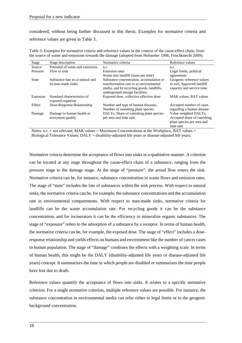
considered, without being further discussed in this thesis. Examples for normative criteria and
reference values are given in Table 3.
Table 3: Examples for normative criteria and reference values in the context of the cause-effect chain, from the source of waste and emissions towards the damage (adopted from Hofstetter 1998, Frischknecht 2009).
Stage Stage description Normative criteria Reference values Source Potential of waste and emissions n.r. n.r. Pressure Flow to sink Emission rates
Waste into landfill [mass per time] Legal limits, political agreements
State Substance fate in a) natural and b) man-made sinks.
Substance concentration, accumulation or transformation rate in a) environmental media, and b) recycling goods, landfills, underground storage facilities.
Geogenic reference values in soil; Approved landfill capacity and service time
Exposure Standard characteristics of exposed organism
Exposed dose, collective effective dose MAK values, BAT values
Effect Dose-Response-Relationship Number and type of human diseases, Number of vanishing plant species
Accepted number of cases regarding a human disease
Damage Damage to human health or ecosystem quality
DALYs, Share of vanishing plant species per area and time unit.
Value weighted DALYs, Accepted share of vanishing plant species per area and time unit
Notes: n.r. = not relevant; MAK values = Maximum Concentrations at the Workplace, BAT values = Biological Tolerance Values; DALY = disability-adjusted life years or disease-adjusted life years;
Normative criteria determine the acceptance of flows into sinks in a qualitative manner. A criterion
can be located at any stage throughout the cause-effect chain of a substance, ranging from the
pressure stage to the damage stage. At the stage of “pressure”, the actual flow enters the sink.
Normative criteria can be, for instance, substance concentration in waste flows and emission rates.
The stage of “state” includes the fate of substances within the sink process. With respect to natural
sinks, the normative criteria can be, for example, the substance concentrations and the accumulation
rate in environmental compartments. With respect to man-made sinks, normative criteria for
landfills can be the waste accumulation rate. For recycling goods it can be the substance
concentration, and for incinerators it can be the efficiency to mineralize organic substances. The
stage of “exposure” refers to the adsorption of a substance by a receptor. In terms of human health,
the normative criteria can be, for example, the exposed dose. The stage of “effect” includes a dose-
response relationship and yields effects on humans and environment like the number of cancer cases
in human population. The stage of “damage” combines the effects with a weighting scale. In terms
of human health, this might be the DALY (disability-adjusted life years or disease-adjusted life
years) concept. It summarizes the time in which people are disabled or summarizes the time people
have lost due to death.
Reference values quantify the acceptance of flows into sinks. It relates to a specific normative
criterion. For a single normative criterion, multiple reference values are possible. For instance, the
substance concentration in environmental media can refer either to legal limits or to the geogenic
background concentration.
18

Proposal for a new indicator
3.4.2 Quantifying critical flows
The critical flow refers to the stage of “pressure” as the actual flow does. To determine the critical
flow rate in mass per time, the actual flow is varied until the associated reference value is achieved.
The causality between the actual flows and the reference values is determined by specific models.
In general the type of model depends on the type and characteristic of the normative criteria. If the
normative criteria are at the stage of “pressure”, the model is rather simple. The critical flow is
either directly given by e.g. law in terms of a flow in mass per time, or it can be calculated based
on legal substance concentration and the actual flow on the level of goods.
The quantification of the critical flow might become more complicated if the normative criteria are
applied at the stage of “state”, “exposure”, “effect” or “damage”. The location determines to what
extent the cause-effectchain has to be analysed. State criteria require fate analysis in the respective
sink. Natural sinks have to be analysed with single-media or multi-media models (Hertwich et al.
2002). Man-made sinks have to be analysed with SFA models that pose an extension of the SFA
model for inventory analysis. For instance, landfills can be investigated (e.g. Laner 2011) in order
to quantify the accumulation rate of substances in the landfill body. Exposure criteria need a
pathway and exposure analysis in view of a certain receptor. The receptor-based approach quantifies
substance concentrations that reach, for instance, people. Exposure scenarios include the
intermediate transfer ratio between the environmental media and the receptor, the uptake factor, the
exposure frequency, duration and an average time for the exposed receptor. Effect criteria require
the definition of a dose-response relationship and yield the effect, for instance, on human health in
terms of number of people affected by cancer. Damage and risk criteria cause the most effort
because analysis refers to the entire cause-effect chain, from the origin source towards the risk for
human and environmental health. In the past, several tools have been developed that quantify risk
criteria including multi-media, exposure and risk analysis (e.g. for human health, see McKone and
Enoch 2002). In this case, an infinite number of critical flows is possible, for instance, as a
consequence of flows into three environmental compartments. To reduce the number of
possibilities, each actual flow is varied while the two others remain constant as long as the reference
values is fulfilled. Accordingly, three actual flows result in three scenarios (A, B, C). The most
stringent scenario is determined by the minimum ratio between the critical and the actual flow, and
becomes selected (Figure 10).
19

Proposal for a new indicator
Figure 10: Each scenario yields a ratio between the critical flow and the actual flow. To select the critical flow for indicator computation, the scenario with the minimum (min) ratio is determinant.
Two general rules are defined for calculating the critical flow:
First, the effort to analyse the cause-effect chain might be reduced if the reference value is achieved
at an earlier stage in the cause-effect chain. For instance, if the legal limits for heavy metal
concentrations in the receiving water (stage of “state”) are already detected in the effluent from the
waste water treatment plant to the receiving water (stage of “pressure”). In this case, the fate
analysis in the environment can be skipped.
Second, the most stringent normative criteria and reference value leads to the least critical flow.
This specification determines the critical flow.
Scenario
Ratio
A B C
min
20

Case studies
4 CASE STUDIES This chapter presents three case studies, including (1) the reasons for selecting these case studies,
(2) the results from inventory analyses, and (3) details about impact assessment. The ultimate result
in terms of the indicator score can be found in chapter 5.
4.1 Selection of case studies The indicator score is calculated in three case studies, including Copper (Cu) and Lead (Pb) on the
city level and Perfluorooctane Sulfonate (PFOS) on the national level (Figure 11). For the metals,
the city level is of relevance because the anthropogenic metal density (mass per spatial unit) in
urban areas is larger than in rural areas (e.g. van Beers et al. 2007). Consequently, urban waste and
emission flows are likely to cause higher metal contents and thus higher sink loads than those in
rural areas. For PFOS, the national level is of relevance because the European Union urges member
states to implement strategies for careful PFOS management. The two metals (Cu and Pb) and the
organic substance (PFOS) have been selected in order to demonstrate the need for different man-
made sinks in dependence on geogenic and man-made substances.
Figure 11: The case studies focus on Cu and Pb on the city level (Vienna) and on PFOS on the national level (Switzerland)
In detail,
• Cu is relevant from both a resource use and environmental impact viewpoint. On the one
hand, Cu is essential for modern lifestyles, resulting in Cu waste fractions that are disposed
of in man-made sinks. From 1900-2000, about 0.7% of the Swiss Cu stock have been
annually discarded to landfills (Wittmer 2006), which pose a future resource deposit. On
the other hand, Cu is emitted from point and non-point sources to natural sinks and poses a
risk for aquatic life. Apart from the rural areas, urban areas are of major relevance. For
instance, in Germany about 30% of total Cu loadings in receiving waters originate from
urban areas (Böhm et al. 2001). In Vienna, Cu concentrations in sewage sludge are
significantly larger than in rural areas (Kroiss et al. 2008), and Cu concentrations in urban
soils are higher than in surrounding rural areas (Pfleiderer 2011).
21

Case studies
• Pb and Pb compound emissions directly affect human health. In Austria, Pb emissions to
air decreased from 218 tons per year (t/yr) in the year 1990 to 13 t/yr in 2009 (Anderl et
al. 2011). In 1993 lead was banned from the Austrian petrol market. It is still used in
accumulators, building coatings, tires and paints. Due to former Pb depositions and present
diffusive losses, anthropogenic Pb is found in urban soils (Kreiner 2004). Hence, it can be
transferred to fodder and food, and may affect human health (WHO 2007).
• Perfluorooctane sulfuric acid and its derivatives, collectively named PFOS, are persistent
bio-accumulative and toxic substances. They are regulated under the Persistent Organic
Pollutants Regulation 850/2004 (European Parliament 2004) and Regulation 2006/122/EG
(European Parliament 2006). In 2010, PFOS has been added to the convention with some
exemptions for specific applications (European Commission 2010). The European Union
(EU) urges member states to implement strategies for careful PFOS management. Even
though Switzerland is a non-EU member state, comprehensive data about anthropogenic
stocks and flows are readily available.
The temporal system boundaries are defined on an annual basis. The reference years include the
years 2007 and 2008 due to data availability.
4.2 Inventory analysis To determine the inventory entries, two steps are needed. (1) The substance flow analysis tool is
applied. (2) The actual flows are selected. This section highlights the results of both steps. Further
details about the calculation including explanations and data are given in article II (Kral et al. 2014)
and article III (Kral et al. 2014).
22
Case studies
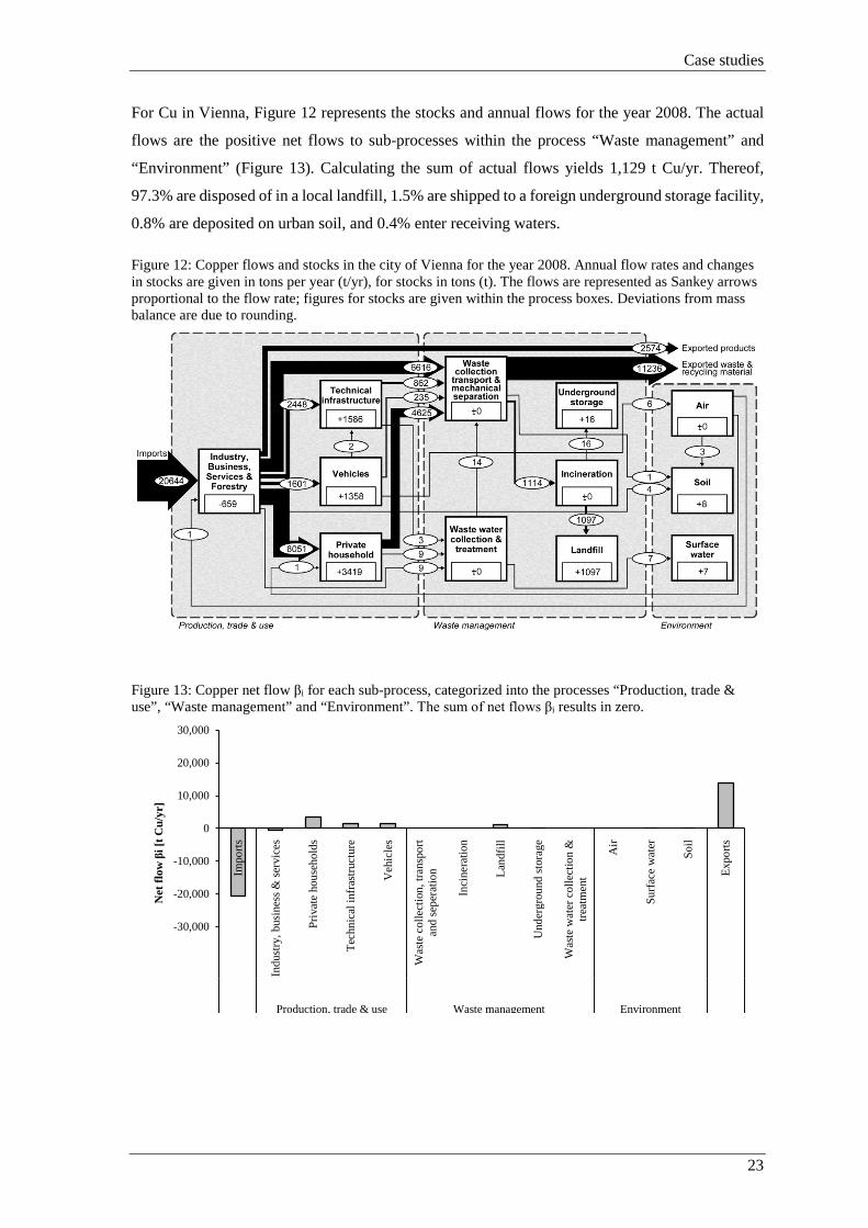
For Cu in Vienna, Figure 12 represents the stocks and annual flows for the year 2008. The actual
flows are the positive net flows to sub-processes within the process “Waste management” and
“Environment” (Figure 13). Calculating the sum of actual flows yields 1,129 t Cu/yr. Thereof,
97.3% are disposed of in a local landfill, 1.5% are shipped to a foreign underground storage facility,
0.8% are deposited on urban soil, and 0.4% enter receiving waters.
Figure 12: Copper flows and stocks in the city of Vienna for the year 2008. Annual flow rates and changes in stocks are given in tons per year (t/yr), for stocks in tons (t). The flows are represented as Sankey arrows proportional to the flow rate; figures for stocks are given within the process boxes. Deviations from mass balance are due to rounding.
Figure 13: Copper net flow βi for each sub-process, categorized into the processes “Production, trade & use”, “Waste management” and “Environment”. The sum of net flows βi results in zero.
-30,000
-20,000
-10,000
0
10,000
20,000
30,000
Impo
rts
Indu
stry
, bus
ines
s & se
rvic
es
Priv
ate
hous
ehol
ds
Tech
nica
l inf
rast
ruct
ure
Veh
icle
s
Was
te c
olle
ctio
n, tr
ansp
ort
and
sepe
ratio
n
Inci
nera
tion
Land
fill
Und
ergr
ound
stor
age
Was
te w
ater
col
lect
ion
&tre
atm
ent
Air
Surf
ace
wat
er
Soil
Expo
rts
Production, trade & use Waste management Environment
Net
flow
βi [
t Cu/
yr]
23

Case studies
For Pb in Vienna, Figure 14 represents the stocks and annual flows for the year 2008. The actual
flows are the positive net flows to sub-processes within the process “Waste management” and
“Environment” (Figure 15). Calculating the sum of actual flows yields the sum of actual flows with
191 t Pb/yr, of which 75.4% entered a local landfill, 22.9% entered a foreign underground storage
facility, 0.8% entered ambient air, 0.5% entered urban soil, and 0.3% entered receiving waters.
Figure 14: Lead flows and stocks in the city of Vienna for the year 2008. Annual flow rates and changes in stocks are given in tons per year (t/yr), for stocks in tons (t). The flows are represented as Sankey arrows proportional to the flow rate; figures for stocks are given within the process boxes. Deviations from mass balance are due to rounding.
Figure 15: Lead net flow βi for each sub-process, categorized into the processes “Production, trade & use”, “Waste management” and “Environment”. The sum of net flows βi results in zero.
-2500
-2000
-1500
-1000
-500
0
500
1000
1500
2000
2500
Impo
rts
Indu
stry
, bus
ines
s & se
rvic
es
Priv
ate
hous
ehol
d
Tech
nica
l inf
rast
ruct
ure
Veh
icle
s
Was
te c
olle
ctio
n, tr
ansp
ort a
ndse
pera
tion In
cine
ratio
n
Land
fill
Und
ergr
ound
stor
age
Was
te w
ater
col
lect
ion
&tre
atm
ent
Air
Surf
ace
wat
er
Soil
Expo
rts
Production, trade & use Waste management Environment
Net
flow
βi [
t Pb/
yr]
24

Case studies
For PFOS in Switzerland, Figure 16 represents the stocks and annual flows for the year 2007. The
actual flows are the positive net flows to sub-processes within the process “Waste management”
and “Environment” (Figure 16). Calculating the sum of actual flows yields 2,260 kg PFOS/yr, of
which 77.1% entered incineration, 0.4% entered landfills, and 22.5% entered geogenic sinks within
the hydrosphere, atmosphere and soil.
Figure 16: PFOS flows and stocks in Switzerland for the year 2007. Annual flow rates and changes in stocks are given in kilograms per year (kg/yr), for stocks in kilograms (kg). The flows are represented as Sankey arrows proportional to the flow rate; figures for stocks are given within the process boxes. Deviations from mass balance are due to rounding.
Figure 17: PFOS net flow βi for each sub-process, categorized into the processes “Production, trade & use”, “Waste management” and “Environment”.The sum of net flows βi results in zero.
-1500
-1000
-500
0
500
1000
1500
2000
Impo
rts
Fire
-figh
ting
foam
stor
age
App
licat
ion
Serv
ice
life
End
-of-l
ife
Recy
clin
g
Sew
erag
e
Inci
nera
tion
Was
te w
ater
trea
t. pl
ant
Land
fill
Surf
ace
wat
er Air
Soil
Exp
orts
Production, trade & use Waste management Environment
Net
flow
βi
[kg
PFO
S/yr
]
25
Case studies
4.3 Impact assessment The chapter includes (1) the selection of normative criteria and reference values, and (2) the
calculation of the critical flows. Further details about the calculation including explanations and
data are given in article III (Kral, Brunner et al. 2014).
4.3.1 Selecting normative criteria and reference values
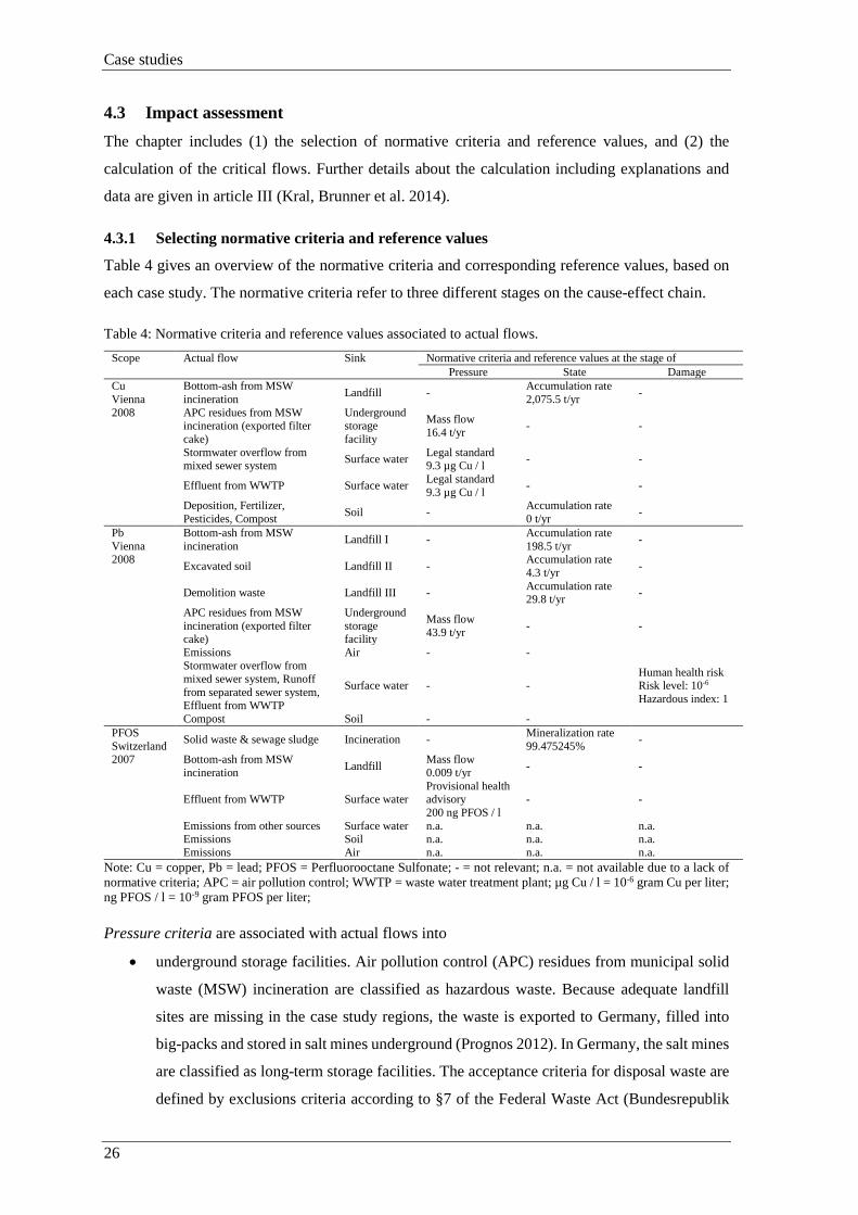
Table 4 gives an overview of the normative criteria and corresponding reference values, based on
each case study. The normative criteria refer to three different stages on the cause-effect chain.
Table 4: Normative criteria and reference values associated to actual flows. Scope Actual flow Sink Normative criteria and reference values at the stage of
Pressure State Damage Cu Vienna 2008
Bottom-ash from MSW incineration Landfill - Accumulation rate
2,075.5 t/yr -
APC residues from MSW incineration (exported filter cake)
Underground storage facility
Mass flow 16.4 t/yr - -
Stormwater overflow from mixed sewer system Surface water Legal standard
9.3 µg Cu / l - -
Effluent from WWTP Surface water Legal standard 9.3 µg Cu / l - -
Deposition, Fertilizer, Pesticides, Compost Soil - Accumulation rate
0 t/yr -
Pb Vienna 2008
Bottom-ash from MSW incineration Landfill I - Accumulation rate
198.5 t/yr -
Excavated soil Landfill II - Accumulation rate 4.3 t/yr -
Demolition waste Landfill III - Accumulation rate 29.8 t/yr -
APC residues from MSW incineration (exported filter cake)
Underground storage facility
Mass flow 43.9 t/yr - -
Emissions Air - -
Human health risk Risk level: 10-6 Hazardous index: 1
Stormwater overflow from mixed sewer system, Runoff from separated sewer system, Effluent from WWTP
Surface water - -
Compost Soil - - PFOS Switzerland 2007
Solid waste & sewage sludge Incineration - Mineralization rate 99.475245% -
Bottom-ash from MSW incineration Landfill Mass flow
0.009 t/yr - -
Effluent from WWTP Surface water Provisional health advisory 200 ng PFOS / l
- -
Emissions from other sources Surface water n.a. n.a. n.a. Emissions Soil n.a. n.a. n.a. Emissions Air n.a. n.a. n.a.
Note: Cu = copper, Pb = lead; PFOS = Perfluorooctane Sulfonate; - = not relevant; n.a. = not available due to a lack of normative criteria; APC = air pollution control; WWTP = waste water treatment plant; µg Cu / l = 10-6 gram Cu per liter; ng PFOS / l = 10-9 gram PFOS per liter; Pressure criteria are associated with actual flows into
• underground storage facilities. Air pollution control (APC) residues from municipal solid
waste (MSW) incineration are classified as hazardous waste. Because adequate landfill
sites are missing in the case study regions, the waste is exported to Germany, filled into
big-packs and stored in salt mines underground (Prognos 2012). In Germany, the salt mines
are classified as long-term storage facilities. The acceptance criteria for disposal waste are
defined by exclusions criteria according to §7 of the Federal Waste Act (Bundesrepublik
26

Case studies
Deutschland 2009). Assuming that the disposal practice complies with German law, it is
just a question of societal and political acceptance in the exporting region if the APC
residues should be disposed of in underground salt mines. This acceptance is given in the
case study regions. Both Switzerland and Vienna agree to the waste export. So, the entire
flow into the man-made sink is classified as accepted, which is in accordance with the
Ecological Scarcity method (Frischknecht, Steiner et al. 2009).
• surface waters. Cu in Vienna enters the River Danube via storm water overflow from the
mixed sewer system and effluents from WWTP. The normative criterion is the Cu
concentration in the water flow, and the reference value is determined with 9.3*10-6 gram
Cu per liter water in accordance with environmental standards (Republik Österreich 2006).
PFOS in Switzerland is detected in effluents from WWTP. Swiss limits regarding PFOS
concentrations are actually missing but under development (Götz et al. 2011).
Consequently, the reference value of 200*10-9 gram PFOS per liter water is based on the
provisional health advisory for drinking water, published by U.S. EPA (2009).
State criteria are associated with actual flows into
• landfills. The acceptance for waste flows into sanitary landfills is defined in national waste
acts. According to the Swiss (Schweizer Bundesrat 2011) and Austrian (Republik
Österreich 2008) regulation, the acceptance includes waste quality criteria such as the
organic carbon content, calorific value, the share of soluble salts, and heavy metal
concentrations. However, these regulations determine possible pressure criteria. They are
not used in the case studies because data quantity and quality regarding waste
characteristics were not available to its’ full extent. For Cu and Pb in Vienna, multiple
proxy criteria are replaced by a single state criteria, which is determined by the constraints
imposed by official permits for each landfill. The normative criteria is the waste
accumulation rate in the landfill. The reference value is quantified by relating the approved
and remaining landfill volume to the remaining service time.
• soil. The Swiss Regulation on the Impact on Soils (Schweizer Bundesrat 1998) aims to
ensure long-term soil fertility. Accumulation of heavy metals in soil is not accepted.
Consequently, the criterion is the accumulation rate in soil, and the reference value is set at
zero. This approach is in accordance with the Ecological Scarcity Method (Frischknecht,
Steiner et al. 2009) and is selected for the case studies due to a lack of more precise data.
• incinerators. The criterion is determined by the efficiency of the thermal treatment process
to mineralize PFOS. The reference value is the mineralization rate, which stands for the
mineralized PFOS mass fraction in relation to the entire PFOS flow into the incinerator.
27

Case studies
Damage criteria are associated with actual flows into air, surface water and soil. For Pb in Vienna,
the flows into natural sinks are assessed in view of human health risks. In accordance with McKone
and Enoch (2002), the Risk Level (RL) and the Hazardous Index (HI) are selected as normative
criteria. The RL considers carcinogenic risk, and the HI non-carcinogenic risk on human health. To
demonstrate the method, widely-used acceptable risks of 10-6 for RL and 1 for HI are selected as
reference values, without discussing further acceptable risks (Kelly 1991).
No criteria are associated with actual flows without available criteria, for instance, as a consequence
of missing data or legal standards. Due to the lack of regulations and standards, the PFOS flows
into soil, air and partly into water are excluded from impact assessment. Nevertheless, the inventory
includes these flows for calculating the sum of actual flows.
4.3.2 Quantifying critical flows
To determine the critical flows in mass per time, the actual flow is varied as long as the associated
reference value is achieved. The link between the actual flows and the reference values is presented
for each criterion:
Pressure criteria refer to flows into
• underground storage facilities. The critical flow is equal to the actual flow [mass per time]
(see chapter 4.3.1).
• surface waters. To calculate the critical flow, the reference value [mass per volume] is
multiplied by the amount of water [volume] to surface waters.
State criteria refer to flows into
• landfills. The critical flow is equal to the accepted waste accumulation rate in the respective
landfill. The accepted rate is defined as the available landfill volume [volume], multiplied
with a specific waste density [mass per volume] and divided by the remaining service time
for disposal [time].
• soil. The accumulation rate of Pb and Cu in soil is set at zero. To achieve this reference
value, the inflow balances the outflow [mass per time]. According to the Ecological
Scarcity method, the critical flow into soil is equal to the uptake of heavy metals by plants.
The calculation of the uptake by plants is based on land use and plant uptake data. This
simplified approach, which neglects leaching from the soil, is justified due to a lack of more
precise data.
• incinerators. To calculate the critical flow, the PFOS flow [mass per time] into the
incinerator is multiplied by the mineralization rate [percent].
28

Case studies
Damage criteria refer to Pb flows into air, soil and water. The risk assessment model CalTOX 4.0
beta (McKone and Enoch 2002) has been developed to assess human exposures from continuous
emissions to multiple environmental media. The model is used to quantify both the damage criteria
RL and the HI. To calculate the critical flows, the actual flows are varied as long as the damage
criteria result in the predefined reference values (see chapter 4.3.1). Each scenario is based on the
variation of a one actual flow out of three, while the two remaining flows are kept constant. Each
variation results in two critical flows. One meets the acceptable RL, another meets the acceptable
HI. To conclude, three actual flows result in six scenarios. The minimum ratio between the critical
flow and the actual flow represents the most stringent scenario, which determines the selection of
the critical flow.
29


Results and discussion
5 RESULTS AND DISCUSSION The chapter gives answers to the research question raised in chapter 1.2.
5.1 What are substance flows to sinks? The physical movement of substances between single processes is called substance flow, whereas
the unit is mass per time (Brunner and Rechberger 2004). A process stands for the accumulation,
transport and transformation of substances, thereby located in the anthroposphere or environment.
A “sink” is a process too. The term is widely used in environmental chemistry and waste
management (see appendix I). With respect to the definitions already given, a new definition is
given for the term “sink” with "a process that accommodates materials that have been removed or
lost from the anthroposphere". Natural sinks are part of biogeochemical cycles (e.g. Abeles et al.
1971, Molina et al. 1974, ICSU 1989, Paterson et al. 1996, Fong et al. 2000, Berg et al. 2004,
Feichter 2008, Yanai et al. 2013). Man-made sinks include technologies such as incinerators,
sanitary landfills, and sewage treatment plants (e.g. Brunner 1999, Vogg 2004, Zeschmar-Lahl
2004, Morf et al. 2005, Brunner et al. 2012, Heiskanen 2013). In a time perspective, the material
can be temporarily or permanently excluded from the anthropogenic material cycle. Temporarily
refers, for instance, to waste stored in landfills (Bertram 2012) that might become a valuable
resource in the future (e.g. Johansson 2013) or to substances stored in environmental media that
might re-enter the anthropogenic material cycle (e.g. Salomons 1998, Bogdal et al. 2009).
Permanently refers, for instance, to organic substances that are mineralized in incinerators (e.g. Van
Caneghem et al. 2010).
5.2 How can the indicator be defined and quantified? The indicator assesses substance flows to regional sinks, caused by the removal and loss of
substances from the anthroposphere. With respect to a specific substance, region and period, the
indicator quantifies the relative magnitude between acceptable and entire flows to regional sinks.
The indicator score is dimensionless, ranging from 0% to 100%. Achieving 100% means that the
total mass of a substance within flows to regional sinks is acceptable. Less than 100% means that
there is a certain mass fraction within flows to regional sinks that overshoot accepted quality
standards. Consequently, the increase of the indicator score up to 100% is seen as good and worth
striving for.
The calculation of the indicator score includes inventory analysis based on substance flow analysis,
and impact assessment based on a distance-to-target approach. The inventory provides actual flows
to sinks, whereas the impact assessment provides acceptable flows to sinks. The aggregation of
single flows results in the proposed indicator.
31

Results and discussion
5.3 What is the indicator score for selected case studies? This chapter presents the case study results by giving (1) a brief overview across all case studies,
and (2) details on an individual case study basis.
5.3.1 Overview
The major results refer to the indicator score λ, which quantifies acceptable mass share in flows to
regional sinks (Figure 18). The indicator score is 99% for Cu in Vienna, 92% for lead in Vienna,
and 96% for PFOS in Switzerland.
Figure 18: Indicator score λ, given in percent (%), for each case study.
Table 5 includes the results from inventory analysis (actual flows), impact assessment (critical and
acceptable flows), and lists the ratio between acceptable and actual flows. Therefore, the Cu
metabolism in Vienna is limited by the storm water overflow from the mixed sewer system to
receiving waters and by flows to urban soil. The Pb metabolism in Vienna is mainly constrained by
excavated soil flows into landfills. The PFOS metabolism in Switzerland partly lacks normative
assessment due to lack of data.
99.0% 92.1% 96.0%
0%
100%
CopperVienna2008
LeadVienna2008
PFOSSwitzerland
2007
Non-assessed mass share in flows to regional sinksUnacceptable mass share in flows to regional sinksAcceptable mass share in flows to regional sinks
32

Results and discussion
Table 5: Results from inventory analysis and impact assessment, on a case study base. Case study
Sink Actual flow name Actual flow
Fi [t/yr]
Critical flow
Fc,i [t/yr]
Acceptable flow
Fa,i [t/yr]
Ratio Fa,ito Fi []
Cu Landfill Bottom-ash from MSW incineration 1,097.2 2,075.5 1,097.2 1.00 Underground
storage facility APC residues from MSW incineration (exported filter cake) 16.4 16.4 16.4 1.00
Surface water Stormwater overflow from mixed sewer system 3.9 0.3 0.3 0.08 Surface water Effluent from WWTP 1.6 1.7 1.6 1.00 Soil Deposition, Fertilizer, Pesticides, Compost 8.8 1.1 1.1 0.13 Sum 1,127.9 - 1,116.6 0.99 Pb Landfill I Bottom-ash from MSW incineration 94.7 198.5 94.7 1.00 Landfill II Excavated soil 17.3 4.3 4.3 0.25 Landfill III Demolition waste 31.9 29.8 29.8 0.93 Underground
storage facility APC residues from MSW incineration (exported filter cake)
43.9 43.9 43.9 1.00
Air Emissions 1.6 6.1 1.6 1.00 Surface water Stormwater overflow from mixed sewer system
Runoff from separated sewer system Effluent from WWTP
0.6 0.6 0.6 1.00
Soil Compost 1.0 1.0 1.0 1.00 Sum 190.9 - 175.8 0.92 PFOS Incineration Solid waste and sewage sludge 1.744 1.744 1.744 1.00 Landfill Bottom-ash from MSW incineration 0.009 0.009 0.009 1.00 Surface water Effluent from WWTP 0.420 0.737 0.420 1.00 Surface water Emissions from other sources 0.060 n.a. n.a. n.a. Soil Emissions 0.029 n.a. n.a. n.a. Air Emissions 0.001 n.a. n.a. n.a. Sum 2.263 - 2.173 0.96
Note: - = not relevant, APC = air pollution control; WWTP = Waste water treatment plant; MSW = municipal solid waste
In the following chapters, the results are discussed on a case study basis, for Cu in Vienna in 2008,
for Pb in Vienna for 2008, and for PFOS in Switzerland in 2007.
33

Results and discussion
5.3.2 Cu in Vienna
In Vienna, 99.0% of Cu flows to regional sinks are acceptable. The sink “soil” poses a constraint
for 0.7% of all actual Cu flows only. The sink “surface water” poses a constraint for 0.3% of all
actual Cu flows.
Figure 19: Case study results from inventory analysis (actual flows) and impact assessment (acceptable and critical flows) regarding Cu in Vienna for the year 2008.
The following results have been obtained (Figure 19), whereas the percentage numbers refer to the
sum of actual flows (100%≙1.128 t/yr):
• Landfill: 97.3% of flows are due to bottom-ash from MSW incineration. This is in
compliance with landfill regulation. Calculated by means of the approved volume and service
time of the landfill, the critical flow is 189% higher than the actual flow. Consequently, there
is no constraint for the disposal of bottom-ash until the end of the approved service time.
• Underground storage facility: 1.5% of flows are due to APC residues from MSW
incineration. These residues are exported and disposed of in approved underground storage
facilities.
• Water: 0.1% of flows are from effluents from the waste water treatment plant (WWTP),
fulfilling quality standards for surface waters. However, the actual flow is only 6% below the
critical flow. Besides WWTP effluents, 0.3% of flows are within storm water overflow from
mixed sewer systems to receiving waters. Applying the same standards as for effluents shows
that the actual flow is 11 times higher than the critical flow.
• Soil: 0.1% of flows are acceptable for urban soil. 0.7% of flows are unacceptable because
they exceed the critical level by a factor of eight. Cu flows into the soil are higher than those
caused by removal by plants. If no Cu leaching from soil is assumed, Cu will accumulate in
specific soil compartments. The determination of the critical flow was rather crude due to a
lack of accurate local data.
0.1
1.0
10.0
100.0
1000.0
10000.0
Bottom-ash frommunicipal solid waste
incineration
APC residues fromMSW incineration
Stormwater overflowfrom mixed sewer
system
Effluent from wastewater treatment plant
DepositionFertilizerPesticidesCompost
Landfill Underground storage Surface water Surface water Soil
Man-made sinks Natural sinks
Cop
per
flow
[t/y
r]
Actual flow
Critical flow
Acceptable flow
34
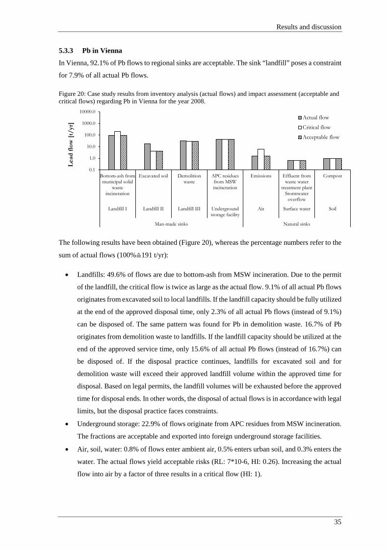
Results and discussion
5.3.3 Pb in Vienna
In Vienna, 92.1% of Pb flows to regional sinks are acceptable. The sink “landfill” poses a constraint
for 7.9% of all actual Pb flows.
Figure 20: Case study results from inventory analysis (actual flows) and impact assessment (acceptable and critical flows) regarding Pb in Vienna for the year 2008.
The following results have been obtained (Figure 20), whereas the percentage numbers refer to the
sum of actual flows (100%≙191 t/yr):
• Landfills: 49.6% of flows are due to bottom-ash from MSW incineration. Due to the permit
of the landfill, the critical flow is twice as large as the actual flow. 9.1% of all actual Pb flows
originates from excavated soil to local landfills. If the landfill capacity should be fully utilized
at the end of the approved disposal time, only 2.3% of all actual Pb flows (instead of 9.1%)
can be disposed of. The same pattern was found for Pb in demolition waste. 16.7% of Pb
originates from demolition waste to landfills. If the landfill capacity should be utilized at the
end of the approved service time, only 15.6% of all actual Pb flows (instead of 16.7%) can
be disposed of. If the disposal practice continues, landfills for excavated soil and for
demolition waste will exceed their approved landfill volume within the approved time for
disposal. Based on legal permits, the landfill volumes will be exhausted before the approved
time for disposal ends. In other words, the disposal of actual flows is in accordance with legal
limits, but the disposal practice faces constraints.
• Underground storage: 22.9% of flows originate from APC residues from MSW incineration.
The fractions are acceptable and exported into foreign underground storage facilities.
• Air, soil, water: 0.8% of flows enter ambient air, 0.5% enters urban soil, and 0.3% enters the
water. The actual flows yield acceptable risks (RL: 7*10-6, HI: 0.26). Increasing the actual
flow into air by a factor of three results in a critical flow (HI: 1).
0.1
1.0
10.0
100.0
1000.0
10000.0
Bottom-ash frommunicipal solid
wasteincineration
Excavated soil Demolitionwaste
APC residuesfrom MSWincineration
Emissions Effluent fromwaste water
treatment plantStormwater
overflow
Compost
Landfill I Landfill II Landfill III Undergroundstorage facility
Air Surface water Soil
Man-made sinks Natural sinks
Lead
flow
[t/y
r]
Actual flow
Critical flow
Acceptable flow
35

Results and discussion
5.3.4 PFOS in Switzerland
In Switzerland, 96.0% of PFOS flows to regional sinks are acceptable. 4% of all actual PFOS flows
lack normative assessment due to insufficient knowledge.
Figure 21: Case study results from inventory analysis (actual flows) and impact assessment (acceptable and critical flows) regarding PFOS in Switzerland for the year 2007.
The following results have been obtained (Figure 21), whereas the percentage numbers refer to the
sum of actual flows (100%≙2.260 t/yr):
• Incineration: 77.1% of PFOS flows originate from solid waste and sewage sludge and are
treated by MSW incineration. This flow is mineralized and is classified as acceptable flow,
which is in accordance with the EU Regulation (European Commission 2010).
• Landfill: 0.4% of flows derive from residues of waste incineration and enter landfills in an
acceptable manner. Today’s PFOS emissions from landfills result from former rather than
from present waste disposal. They have been assessed as well.
• Water: Two flows enter the aquatic sphere. 18.6% of PFOS are within WWTP effluents and
fulfill provisional drinking water standards (U.S. EPA 2009). Up to now in Switzerland, legal
limits have been lacking but are under development (Götz, Kase et al. 2011). 2.7% of PFOS
originate from additional sources. This flow has not been assessed because data and standards
were missing.
• Soil and air: 1.3% of PFOS enter the soil, and 0.04% enter air. These flows, together with the
2.7% of flows into water, have not been assessed due to a lack of data.
0.1
1.0
10.0
100.0
1000.0
10000.0
Solid waste &sewage sludge
Bottom-ash frommunicipal solid
waste incineration
Effluent from wastewater treatment
plant
Emissions fromother sources
Emissions Emissions
Incineration Landfill Surface water Surface water Soil Air
Man-made sinks Natural sinks
PFO
S flo
w [t
/yr]
Actual flowCritical flowAcceptable flowActual flow without normative assessment
36
Results and discussion
5.4 What’s the benefit of the new indicator? The benefits of the new indicator refer (i) to implications of the case study findings on waste and
environmental management, (ii) to the relevance of the indicator score, and (iii) to implications of
the proposed indicator on resource use in general.
First, the three substances taken into account are widely present in the respective regions, but appear
to include fractions that exceed quality standards. For each substance, proactive strategies and
measures are needed to increase the indicator score up to 100% in the future.
• For Cu in Vienna, the deposition on urban soil exceeds the acceptance level by a factor of
eight. Due to a lack of local data and non-site-specific assessment criteria, the assessment is
rather crude. Consequently, the quantity and quality of data has to be improved. This finding
is in agreement with the recommendation of the Austrian Environmental Agency for a nation-
wide monitoring program for metals in soil (Umweltbundesamt 2010). Based on the case study
findings, two measures are recommended: On the one hand, improved sampling with respect
to horizontal and vertical sample collection, and including the identification of potential hot
spots, would allow a decrease in the uncertainty when determining the amount of critical flows
to the soil. On the other hand, the development and definition of site-specific reference values
in terms of substance concentrations for urban soil are needed. The stormwater overflow into
receiving waters exceeds the quality standards by a factor of 11. The stormwater overflow was
estimated with a combined water and copper balance model for Vienna, calibrated on the
inflow to the waste water treatment plant. Enhanced data quality will improve the
quantification of the storm water overflow. For the future, the indicator score might increase
due to ongoing measures for reducing water bypassing waste water treatment via storm water
overflow (e.g. Stadt Wien 2013).
• For Pb in Vienna, the flow into landfill exceeds the approved landfill capacity before the
service time runs out. To overcome these constraints, landfill permits might be extended in
time. Alternatively, wastes are directed to remote landfills beyond the system limits, which
increases transport distances and costs, or waste fractions can be recycled, complying with
advanced quality standards (BRV 2009). Even though the flows into natural sinks yield
acceptable human health risks, it has to be noted that the method is based on a uniform
approach without spatial resolution. Thus, accidental hot spots representing possible risks for
the local population are not included in this approach.
• For PFOS in Switzerland, some flows into air, soil and water have not been assessed due to a
lack of data. These flows still pose risks for human and environmental health. For most
applications PFOS has been banned, but PFOS still hibernates in present stocks due to former
imports. So, PFOS will continue to enter waste flows, whereas the monitoring of PFOS is
37

Results and discussion
rather challenging and expensive (e.g. Schultz et al. 2006, Becker et al. 2008). Due to the
obligation to destroy or irreversibly transform the POP content (European Parliament 2004) to
PFOS for waste, the concentrations might exceed regulated concentration limits. This effects
recycling systems, which “may challenge another environmental priority of ensuring the
sustainable use of resources” (European Commission 2010).
Second, the indicator score is of relevance because it fulfills three needs according to Frederiksen
and Gudmundsson (2013): First, a need of governments, institutions and companies to satisfy
transparency and accountability requirements in policy and measure performance evaluation. The
temporal alignment of the indicator score appears to represent the effects of measures undertaken.
Second, a need to compare the performance of environmental and waste management across
regions. Third, a need to communicate scientific research to the public and decision makers on
environmental quality. The indicator processes complex information about the quantity and quality
of anthropogenic material flows into an easily understandable score.
Third, materials are removed or lost from the anthroposphere. To accommodate these material
without burdens on human and environmental health, natural sinks are available to a certain extent,
and man-made sinks have to be provided where natural sinks are missing or lacking. If appropriate
sinks are not available, for instance, as a consequence of technological and economic feasibility or
ineffective policy instruments, there is a need for strategies that change the anthropogenic material
turnover in terms of quantity or quality. The proposed indicator diagnoses to which extent sinks are
loaded in an acceptable manner. This information is of major relevance for strategies managing
materials that leave the anthroposphere to regional sinks.
38

Future research and outlook
6 FUTURE RESEARCH AND OUTLOOK Investigating the regional material turnover is (a) needed to manage material stocks and flows with
respect to quality criteria, and is (b) required to identify the need for sinks in external regions and
to develop suitable strategies to monitor and control external sink loads. Future research is needed
to evaluate the flow “exported waste & recycling material” (see figure 4). It crosses the spatial
system boundary and enters external regions. It might be that the flow is not acceptable due to the
same constraints as in the exporting region, for instance, because it surpasses standards for pollution
control or overloads the sink “sanitary landfill”. The relevance of waste exports fraught with risk is
well documented, for example, for electrical and electronic equipment waste (e.g. Widmer et al.
2005, Sthiannopkao et al. 2013). With respect to the case studies, the flow “exported waste &
recycling material” to external sinks is not taken into account, except those to underground storage
facilities. To allocate export flows to the exporting region, critical flows for flows within “export
waste & recycling material” must be defined. In other words, the removal and loss of substances
from exported flows to external sinks must be considered. Therefore, the spatial system boundary
has to be extended by including the hinterland. In this case, the proposed method for assessing
substance flows to regional sinks is applied for the external regions too. After the critical flow has
been determined, the exporting region might increase the critical flow by a marked based trading
scheme. The proposed scheme allocates external sink loads to the exporting region. This
management option is inspired by the mechanism under the Kyoto Protocol (see chapter 2.3).
Therefore, allocation procedures are based on tradable permits, including trading units for reducing
emissions and enhancing appropriate sinks capacities in external regions. In the context of the flow
“exported waste & recycling material”, the critical flows might be increased by reducing emissions
or enhancing appropriate sink capacities in the external region. Of course, the proposed
management option is visionary, but it respects a globally integrated economy that exchanges
wastes and recyclables across regions.
39


References
REFERENCES Abeles, F. B., L. E. Craker, L. E. Forrence, et al. 1971. Fate of Air Pollutants: Removal of Ethylene, Sulfur Dioxide, and Nitrogen Dioxide by Soil. Science 173(4000): 914-916. Adriaanse, A., S. Bringezu, A. Hammond, et al. 1997. Resource Flows: The Material Basis of Industrial Economies. Washington, DC: World Resource Institute. Alfsen, K. and H. Sæbø. 1993. Environmental quality indicators: Background, principles and examples from Norway. Environmental and Resource Economics 3(5): 415-435. Anderl, M., M. Gangl, S. Göttlicher, et al. 2011. Emissionstrends 1990-2009. Ein Überblick über die österreichischen Verursacher von Luftschadstoffen. [Emission trends 1990-2009. An overview about airborne emission sources in Austria.] Wien: Umweltbundesamt. Anderl, M., M. Gangl, H. Jobstmann, et al. 2013. Emissonstrends 1990-2011. Ein Überblick über die österreichischen Versursacher von Luftschadstoffen. [Emission trends 1990-2011. An overview about airborne emission sources in Austria.] Wien: Umweltbundesamt. Azar, C., J. Holmberg and K. Lindgren. 1996. Socio-ecological indicators for sustainability. Ecological Economics 18(2): 89-112. Baccini, P. and H. P. Bader. 1996. Regionaler Stoffhaushalt. [Regional Metabolism.] Heidelberg, Berlin, Oxford: Spektrum, Akad. Verlag. Baccini, P. and P. H. Brunner. 1991. Metabolism of the Anthroposphere. New York: Springer. Becker, A. M., S. Gerstmann and H. Frank. 2008. Perfluorooctane surfactants in waste waters, the major source of river pollution. Chemosphere 72(1): 115-121. Berg, B. and N. Dise. 2004. Calculating the long-term stable nitrogen sink in northern European forests. Acta Oecologica 26(1): 15-21. Berg, M. and M. Scheringer. 1994. Problems in Environmental Risk Assessment and the Need for Proxy Measures. Fresenius Environmental Bulletin 3(8): 487-492. Bertram, H. U. 2012. Landfills as pollution sink in an environmentally sound recycling management. In Waste Management, Volume 3. Recycling and Recovery, edited by K. J. Thomé-Kozmiensky and S. Thiel. Neuruppin: TK Verlag Karl Thomé-Kozmiensky. Boesch, M. E., A. Koehler and S. Hellweg. 2009. Model for cradle-to-gate life cycle assessment of clinker production. Environ Sci Technol 43(19): 7578-7583. Boesch, M. E., C. Vadenbo, D. Saner, et al. 2014. An LCA model for waste incineration enhanced with new technologies for metal recovery and application to the case of Switzerland. Waste Manag 34(2): 378-389. Bogdal, C., P. Schmid, M. Zennegg, et al. 2009. Blast from the past: melting glaciers as a relevant source for persistent organic pollutants. Environ Sci Technol 43(21): 8173-8177. Böhm, E., T. Hillenbrand, F. Marscheider-Weidemann, et al. 2001. Bilanzierung des Eintrags prioritärer Schwermetalle in Gewässer. [Flows of prioritized heavy metals into reveiving waters.] Berlin: Umweltbundesamt. Brunner, P. H. 1999. In search of the final sink. Environ Sci Pollut Res Int 6(1): 1.
41

References
Brunner, P. H. 2002. Beyond Materials Flow Analysis. Journal of Industrial Ecology 6(1): 8-10. Brunner, P. H. 2010. Clean cycles and safe final sinks. Waste Management & Research 28(7): 575-576. Brunner, P. H. and H. Rechberger. 2004. Practical Handbook of Material Flow Analysis. Boca Raton, Florida: CRC Press. Brunner, P. H. and D. M. Stampfli. 1993. Material Balance of a Construction Waste Sorting Plant. Waste Management & Research 11(1): 27-48. Brunner, P. H. and J. C. Tjell. 2012. Do we need sinks? Waste Manag Res 30(1): 1-2. BRV. 2009. Kurzfassung der Richtlinie für Recycling-Baustoffe. [Guideline for recycling material.] Wien: Baustoff Recycling Verband (BRV). Bundesrepublik Deutschland. 2009. Verordnung über Deponien und Langzeitlager. [Landfill and Long-term Storage Directive.] Burger Chakraborty, L., A. Qureshi, C. Vadenbo, et al. 2013. Anthropogenic mercury flows in India and impacts of emission controls. Environ Sci Technol 47(15): 8105-8113. Buser, A. and L. S. Morf. 2009. Substance flow analysis for Switzerland: Perfluorinated surfactants perfluorooctanesulfonate (PFOS) and perfluorooctanoic acid (PFOA). Bern: Federal Office for the Environment. Cencic, O. 2012. Software platform STAN (short for subSTance flow ANalysis). Vienna Universtiy of Technology. Retrieved 28th September 2012, from www.stan2web.net. Chen, P.-C., H.-J. Su and H.-W. Ma. 2013. Trace anthropogenic arsenic in Taiwan - Substance flow analysis as a tool for environmental risk management. Journal of Cleaner Production 53(0): 13-21. Chen, S. J., Y. J. Ma, J. Wang, et al. 2009. Brominated flame retardants in children's toys: concentration, composition, and children's exposure and risk assessment. Environ Sci Technol 43(11): 4200-4206. Common, M. S. and S. Stagl. 2005. Ecological economics: an introduction. Cambridge: Cambridge University Press. Deutscher Bundesrechnungshof. 2014. Bemerkungen des Bundesrechnungshofes 2013 zur Haushalts- und Wirtschaftsführung des Bundes. [Comments on Federal Economics by the German Court of Auditors.] Bonn. Dittrich, M., S. Giljum, S. Lutter, et al. 2013. Aktualisierung von nationalen und internationalen Ressourcenkennzahlen. [Update of national and international resource indicators.] Dessau-Roßlau: Umweltbundesamt. Döberl, G. and P. H. Brunner. 2004. Substances and their (final) sinks - a new indicator for monitoring sustainability. Paper presented at Indicators for Evaluating Sustainable Development - The Ecological Dimension, 1st - 2nd November 2004, Berlin.
42
References
Döberl, G., R. Huber, P. H. Brunner, et al. 2002. Long-term assessment of waste management options - a new, integrated and goal-oriented approach. Waste Management & Research 20(4): 311-327. EEA. 2012. Environmental indicator report 2012. Copenhagen: European Environment Agency (EEA). ESFA. 2012. Scientific Opinion on Mineral Oil Hydrocarbons in Food. European Food Safety Authority (ESFA) Journal 10(6). European Commission. 2010. Commission Regulation (EU) No 756/2010 of 24 August 2010 amending Regulation (EC) No 850/2004 of the European Parliament and of the Council on persistent organic pollutants as regards Annexes IV and V. European Communities. 2001. Economy-wide material flow accounts and derived indicators - A methodological guide. Luxembourg. European Parliament. 2004. Regulation (EC) No 850/2004 of the European Parliament and of the Council of 29 April 2004 on persistent organic pollutants and amending Directive 79/117/EEC. European Parliament. 2006. Directive 2006/122/ECof the European Parliament and of the Council of 12 December 2006 amending for the 30th time Council Directive 76/769/EEC on the approximation of the laws, regulations and administrative provisions of the Member States relating to restrictions on the marketing and use of certain dangerous substances and preparations (perfluorooctane sulfonates). European Parliament. 2006. Regulation (EC) No 1907/2006 of the European Parliament and of the Council of 18 December 2006 concerning the Registration, Evaluation, Authorisation and Restriction of Chemicals (REACH), establishing a European Chemicals Agency. Feichter, J. 2008. Die Atmosphäre als Schadstoffsenke - Einfluss auf Stoffkreisläufe und Klima. In Industrial Ecology. [The atmosphere as pollution sink - Impact on substance cycles and climate.], edited by A. Gleich and S. Gößling-Reisemann: Vieweg+Teubner. Fong, D. P. and D. J. B. Zedler. 2000. Sources, sinks, and fluxes of nutrients (N + P) in a small highly modified urban estuary in southern California. Urban Ecosystems 4(2): 125-144. Förstner, U. and G. Müller. 1973. Heavy metal accumulation in river sediments: A response to environmental pollution. Geoforum 4(2): 53-61. Frederiksen, P. and H. Gudmundsson. 2013. Policy use and influence of indicators. Ecological Indicators 35(0): 1-2. Frischknecht, R. 2009. Umweltverträgliche Technologien - Analyse und Beurteilung. Teil 2: Ökobilanzen (Skriptum). [Environmental technologies: Analysis and Evaluation. Part 2: Life cycle assessment (Lecture notes).] Zürich: Eigenössische Technische Hochschule Zürich. Frischknecht, R., R. Steiner and N. Jungbluth. 2009. The Ecological Scarcity Method – Eco-Factors 2006. A method for impact assessment in LCA. Bern: Federal Office for the Environment. Gilbert, A. J. and J. F. Feenstra. 1994. A sustainability indicator for the Dutch environmental policy theme ‘Diffusion’: cadmium accumulation in soil. Ecological Economics 9(3): 253-265.
43

References
Goedkoop, M. J., R. Heijungs, M. Huijbregts, et al. 2012. ReCiPe 2008. A life cycle impact assessment method which comprises harmonized category indicators at the midpoint and endpoint level. The Hague: Ministry of Housing Spatial Planning and Environment (VROM). Gottschalk, F., R. W. Scholz and B. Nowack. 2010. Probabilistic material flow modeling for assessing the environmental exposure to compounds: Methodology and an application to engineered nano-TiO2 particles. Environmental Modelling & Software 25(3): 320-332. Götz, C. W., R. Kase and J. Hollender. 2011. Mikroverunreinigungen - Beurteilungskonzept für organische Spurenstoffe aus kommunalem Abwasser. Studie im Auftrag des BAFU. [Micropollutants - Evaluation concept for organic trace substances in municipal waste water. A study conducted by BAFU.] Dübendorf: Eidgenössische Anstalt für Wasserversorgung Abwasserreinigung und Gewässerschutz (EAWAG). Grandjean, P. 2013. Science for precautionary decision-making. In Late lessons from early warnings: science, precaution, innovation, edited by European Environmental Agency. Luxembourg: Publications Office of the European Union. Graymore, M. L. M., N. G. Sipe and R. E. Rickson. 2010. Sustaining Human Carrying Capacity: A tool for regional sustainability assessment. Ecological Economics 69(3): 459-468. Guinée, J. B., J. C. J. M. van den Bergh, J. Boelens, et al. 1999. Evaluation of risks of metal flows and accumulation in economy and environment. Ecological Economics 30(1): 47-65. Hausberger, S. 1997. Globale Modellbildung für Emissions- und Verbrauchsszenarien im Verkehrssektor. [Global Modelling of Scenarios Concerning Emission and Fuel Consumption in the Transport Sector.] PhD Thesis, Graz: Technische Universität Graz. Hedbrant, J. and L. Sörme. 2001. Data Vagueness and Uncertainties in Urban Heavy-Metal Data Collection. Water, Air, & Soil Pollution: Focus 1(3): 43-53. Heiskanen, J. ed. 2013. Sinks, a vital element of modern waste managment. International Solid Waste Association (ISWA) Beacon Conference: 2nd International Conference on Final Sinks, 16-18 May 2013, Espoo: Aalto University. Hellweg, S., T. B. Hofstetter and K. Hungerbuhler. 2005. Time-dependent life-cycle assessment of slag landfills with the help of scenario analysis: the example of Cd and Cu. Journal of Cleaner Production 13(3): 301-320. Hertwich, E., O. Jolliet, D. Pennington, et al. 2002. Fate and Exposure Assessment in the Life-Cycle Impact Assessment of Toxic Chemicals. In Life-Cycle Impact Assessment: Striving Towards Best Practice, edited by H. A. Udo de Haes, S. Kotaji, A. Schuurmans et al. Pensacola, Florida: SETAC Press. Hoekstra, R. and J. C. J. M. van den Bergh. 2006. Constructing physical input–output tables for environmental modeling and accounting: Framework and illustrations. Ecological Economics 59(3): 375-393. Hofstetter, P. 1998. Perspectives in life cycle impact assessment - A structured approach to combine models of the technosphere, ecosphere and valuesphere. PhD Thesis, Zürich: Eigenössische Technische Hochschule Zürich. Hunter, P. R. and L. Fewtrell. 2001. Acceptable risk. In Water Quality: Guidelines, Standards and Health, edited by L. Fewtrell and J. Bartram. London: IWA Publishing,.
44

References
ICSU. 1989. The ocean as a source and sink for atmospheric trace constituents (Final report of SCOR Working Group 72). Paris: International Council of Scientific Unions (ICSU), UNESCO. Jang, E., K.-r. Kim, K.-h. Kim, et al. 2012. Material Flow Analysis and Human Risk Assessment of Mercury. In Design for Innovative Value Towards a Sustainable Society, edited by M. Matsumoto, Y. Umeda, K. Masui et al.: Springer Netherlands. Jesinghaus, J. 1999. A European System of Environmental Pressure Indices. First Volume of the Environmental Pressure Indices Handbook: The Indicators. European Commission, Joint Research Centre, Institute for Systems, Informatics and Safety (ISIS). Retrieved March 2013, from http://esl.jrc.ec.europa.eu/envind/theory/handb_.htm. Johansson, N. 2013. Why don’t we mine the landfills? PhD Thesis, Linköping: Linköping University. Jungbluth, N., S. Busser, R. Frischknecht, et al. 2012. Feasibility of environmental product information based on life cycle thinking and recommendations for Switzerland. Journal of Cleaner Production 28(0): 187-197. Kelly, K. E. 1991. The Myth of 10-6 as a Definition of Acceptable Risk. Paper presented at 84th Annual Meeting Air & Waste Management Association, 16-21 June 1991, Vancouver, BC. Kral, U., P. H. Brunner, P. C. Chen, et al. 2014. Sinks as limited resources? - A new indicator for evaluating anthropogenic material flows. Ecological Indicators: Submitted on January 2014. Kral, U., K. Kellner and P. H. Brunner. 2013. Sustainable resource use requires “clean cycles” and safe “final sinks”. Science of The Total Environment 461–462(0): 819-822. Kral, U., C.-Y. Lin, K. Kellner, et al. 2014. The Copper Balance of Cities. Journal of Industrial Ecology: In press. Kreiner, P. 2004. Wiener Bodenbericht 2003: Untersuchung des Wiener Bodens auf Schwermetalle und polyaromatische Kohlenwasserstoffe. [Viennese soil report 2003: Investigation heavy metals and hydrocarbons in Viennese soils.] Wien: Stadt Wien - Magistratsabteilung 22. Kroiss, H., L. S. Morf, C. Lampert, et al. 2008. Optimiertes Stoffflussmonitoring für die Abwasserentsorgung Wiens. [Optimized substance flow monitoring for the waste water treatment plant in Vienna.] Wien: Technische Universität Wien. Krotscheck, C. and M. Narodoslawsky. 1996. The sustainable process index - A new dimension in ecological evaluation. Ecological Engineering 6(4): 241-258. Laner, D. 2011. Understanding and evaluating long-term environmental risks from landfills. PhD Thesis, Vienna: Vienna University of Technology. Laner, D. and H. Rechberger. 2007. Treatment of cooling appliances: Interrelations between environmental protection, resource conservation, and recovery rates. Resources, Conservation and Recycling 52(1): 136-155. Laner, D. and H. Rechberger. 2009. Quantitative evaluation of waste prevention on the level of small and medium sized enterprises (SMEs). Waste Manag 29(2): 606-613. Lesmes-Fabian, C. and C. R. Binder. 2013. Pesticide flow analysis to assess human exposure in greenhouse flower production in Colombia. Int J Environ Res Public Health 10(4): 1168-1185.
45

References
Lifset, R. J., M. J. Eckelman, E. M. Harper, et al. 2012. Metal lost and found: dissipative uses and releases of copper in the United States 1975-2000. Sci Total Environ 417-418(0): 138-147. Månsson, N., B. Bergbäck, D. Hjortenkrans, et al. 2009. Utility of Substance Stock and Flow Studies. [Utility of Substance Stock and Flow Studies.] Journal of Industrial Ecology 13(5): 674-686. Månsson, N., B. Bergbäck and L. Sörme. 2009. Phasing Out Cadmium, Lead, and Mercury. Journal of Industrial Ecology 13(1): 94-111. McKone, T. E. and K. G. Enoch. 2002. CalTOX (registered trademark), A multimedia total exposure model spreadsheet user's guide. Version 4.0(Beta). California: University of California. Mitchell, G. and C. Diaper. 2010. UVQ User Manual (CMIT Report No. 2005-282). Canberra: Commonwealth Scientific and Industrial Research Organisation. Mohareb, E. and C. Kennedy. 2012. Gross Direct and Embodied Carbon Sinks for Urban Inventories. Journal of Industrial Ecology 16(3): 302-316. Molina, M. J. and F. S. Rowland. 1974. Stratospheric sink for chlorofluoromethanes: chlorine atomc-atalysed destruction of ozone. Nature 249(5460): 810-812. Morf, L. S. and P. H. Brunner. 2005. MVA als Schadstoffsenke - Stoffflussanalyse für Quecksilber im MHKW Würzburg. [Municipal solid waste incineration as sink for substances - Substance flow analysis for Hg in an incinerator at Würzburg.] Wien und Zürich: Technische Universität Wien. Nagl, H. D. 1996. Critical Loads & Levels: Naturwissenschaftliche Bestandteile eines Indikatorensystems für dauerhaft-umweltgerechte Entwicklungen. In Indikatoren einer regionalen nachhaltigen Entwicklung. [Critical Loads & Levels: Science-based indicator systems for environmental development.], edited by G. Pfister and O. Renn. Baden-Württemberg: Akademie für Technikfolgenabscllätzung in Baden-Württemberg. Nic, M., J. Jirát, B. Kosata, et al. 2012. Compendium of chemical terminology (Version 2.3.2). Research Triangle Park, NC: International Union of Pure and Applied Chemistry (IUPAC). Nilsson, J. and S. Bergström. 1995. Indicators for the assessment of ecological and economic consequences of municipal policies for resource use. Ecological Economics 14(3): 175-184. Ott, C. and H. Rechberger. 2012. The European phosphorus balance. Resources Conservation and Recycling 60(0): 159-172. ÖWAV. 2003. Die Anwendung der Stoffflussanalyse in der Abfallwirtschaft (ÖWAV- Regelblatt 514). [The application of the substance flow analysis tool in the waste management sector (ÖWAV - Standard 514).]. Wien: Österreichischer Wasser- und Abfallwirtschaftsverband (ÖWAV). Palm, V. and C. Ostlund. 1996. Lead and zinc flows from technosphere to biosphere in a city region. Science of the Total Environment 192(1): 95-109. Paterson, E., M. Sanka and L. Clark. 1996. Urban soils as pollutant sinks. A case study from Aberdeen, Scotland. Applied Geochemistry 11(1–2): 129-131.
46

References
Pfleiderer, S. 2011. Umweltgeochemie Stadtgebiet Wien. [Environmental geochemistry of the city of Vienna.] Paper presented at Seminar Ressourcenmanagement und Abfallwirtschaft, 4th June 2011, Wien. Prognos. 2012. Perspektiven der Untertage-Entsorgung in Deutschland. [Perspectives on underground storage in Germany.] Berlin: Prognos AG. Rechberger, H. and P. H. Brunner. 2002. A new, entropy based method to support waste and resource management decisions. Environ Sci Technol 36(4): 809-816. Reimann, C., P. Filzmoser and R. G. Garrett. 2005. Background and threshold: critical comparison of methods of determination. Science of the Total Environment 346(1-3): 1-16. Republik Deutschland. 2012. Gesetz zur Förderung der Kreislaufwirtschaft und Sicherung der umweltverträglichen Bewirtschaftung von Abfällen (Kreislaufwirtschaftsgesetz - KrWG). [Federal Recycling Act.]. Republik Österreich. 2006. Verordnung des Bundesministers für Land- und Forstwirtschaft, Umwelt und Wasserwirtschaft über die Festlegung des Zielzustandes für Oberflächengewässer. [Water quality Directive.]. Republik Österreich. 2008. Bundesgesetz über eine nachhaltige Abfallwirtschaft (Abfallwirtschaftsgesetz 2002). [Federal Waste Act 2002.]. Republik Österreich. 2008. Verordnung des Bundesministers für Land- und Forstwirtschaft, Umwelt und Wasserwirtschaft über Deponien (Deponieverordnung 2008). [Landfill Directive.]. Ritthoff, M., H. Rohn, C. Liedtke, et al. 2002. Calculating MIPS: Resource productivity of products and services. Wuppertal, Germany: Wuppertal Institute for Climate Environment and Energy. Rochat, D., C. R. Binder, J. Diaz, et al. 2013. Combining Material Flow Analysis, Life Cycle Assessment, and Multiattribute Utility Theory Assessment of End-of-Life Scenarios for Polyethylene Terephthalate in Tunja, Colombia. Journal of Industrial Ecology 17(5): 642-655. Rubli, S. 2013. Dynamische Modellierung der Asphalt- sowie PAK-Lager und Flüsse in den Strassen der Regiona St. Gallen, Thurgau, Zürich und Fürstentum Liechtenstein. [Dynamic modeling of asphalt and PAH-stocks and flows in roads of the districts St. Gallen, Thurgau, Zürich and the Principality of Liechtenstein.] Schlieren: Energie- und Ressourcen-Management GmbH. Salomons, W. 1998. Biogeodynamics of contaminated sediments and soils: perspectives for future research. Journal of Geochemical Exploration 62(1-3): 37-40. Samsonek, J. and F. Puype. 2013. Occurrence of brominated flame retardants in black thermo cups and selected kitchen utensils purchased on the European market. Food Addit Contam Part A Chem Anal Control Expo Risk Assess 30(11): 1976-1986. Scheringer, M. and M. Berg. 1994. Spatial and temporal range as measures of environemental threat. Fresenius Environmental Bulletin 3: 493-498. Schultz, M. M., D. F. Barofsky and J. A. Field. 2006. Quantitative Determination of Fluorinated Alkyl Substances by Large-Volume-Injection Liquid Chromatography Tandem Mass SpectrometryCharacterization of Municipal Wastewaters. Environmental Science & Technology 40(1): 289-295.
47

References
Schweizer Bundesrat. 1998. Verordnung vom 1. Juli 1998 über Belastungen des Bodens (VBBo). [Regulation on impacts on soil pollution of July 1st, 1998.]. Schweizer Bundesrat. 2011. Technische Verordnung über Abfälle vom 10. Dezember 1990 (Stand am 1. Juli 2011). [Technical Waste Directive from 10th December 1990 (Status 1st July 2011).] Sobańtka, A. 2013. The extension of statistical entropy analysis to chemical compounds. PhD Thesis, Vienna: Vienna University of Technology. Spranger, T., U. Lorenz and H.-D. Gregor. 2004. Manual on methodologies and criteria for Modelling and Mapping Critical Loads & Levels and Air Pollution Effects, Risks and Trends. Berlin: Federal Environmental Agency. Stadt Wien. 2013. Asperner Sammelkanal Entlaster in Bau. [Aspern collection sewer under construction.] Retrieved 14th November 2013, from www.wien.gv.at/umwelt/kanal/baustellen/asperner-sammelkanal-entlaster.html. Sthiannopkao, S. and M. H. Wong. 2013. Handling e-waste in developed and developing countries: initiatives, practices, and consequences. Sci Total Environ 463-464(0): 1147-1153. Stumm, W. and J. Davis. 1974. Kann Recycling die Umweltbeeinträchtigung vermindern? (in German: Does Recylcing minimize environmental impacts?). Recycling: Lösung der Umweltkrise? (in German: Recyling: Solution of Environemental Crisis?): 29-41. U.S. EPA. 2009. Provisional Health Advisories for Perfluorooctanoic Acid (PFOA) and Perfluorooctane Sulfonate (PFOS). U.S. Environmental Protection Agency (U.S. EPA). Retrieved March 2013, from http://water.epa.gov/drink/standards/hascience.cfm. U.S. EPA. 2011. Highlights of the Exposure Factors Handbook. Washington, DC: U.S. Environmental Protection Agency (U.S. EPA). Umweltbundesamt ed. 1999. Umweltindikatoren für Österreich - Regionale und nationale Maßzahlen zur Dokumentation der Umweltsituation auf dem Weg zu einer nachhaltigen Entwicklung. [Environmental indicators for Austria.] Umweltindikatoren für Österreich, 16. -17. November 1998, Schloss Wilheminenberg, Wien. Umweltbundesamt. 2010. Neunter Umweltkontrollbericht - Umweltsituation in Österreich. [9th Environmental report - Austrian situation.] Wien: Umweltbundesamt. UNCHS. 2001. The State of the Worlds Cities 2001. Nairobi: United Nations Centre for Human Settlements (UNCHS). UNCSD. 1996. Working List of Indicators of Sustainable Development. New York: United Nations Commission on Sustainable Development (UNCSD). UNEP. 2013. Metal recycling. Opportunities, Limits, Infrastructure. A Report of the Working Group on the Global Metal Flows to the International Resource Panel. Nairobi: United Nations Environmental Programme (UNEP). UNFCCC. 2008. Kyoto Protocol Referene Manual. On Accounting of Emissions and assigned amount. Bonn: United Nations Framework Convention on Climate Change (UNFCCC). United Nations. 1998. Kyoto Protocol to the United Nations Framework Convention on Climate Change.
48

References
Vadenbo, C. O., M. E. Boesch and S. Hellweg. 2013. Life Cycle Assessment Model for the Use of Alternative Resources in Ironmaking. Journal of Industrial Ecology 17(3): 363-374. van Beers, D. and T. E. Graedel. 2007. Spatial characterisation of multi-level in-use copper and zinc stocks in Australia. Journal of Cleaner Production 15(8-9): 849-861. Van Caneghem, J., C. Block, A. Van Brecht, et al. 2010. Mass balance for POPs in hazardous and municipal solid waste incinerators. Chemosphere 78(6): 701-708. Van der Voet, E. 1996. Substances from cradle to grave : development of a methodology for the analysis of substances flows through the economy and the environment of a region: with case studies on cadmium and nitrogen compounds. PhD Thesis, Leiden University. van der Voet, E., L. van Oers, J. B. Guinee, et al. 1999. Using SFA indicators to support environmental policy. Environ Sci Pollut Res Int 6(1): 49-58. van het Bolcher, M., H. Denier van der Gon, J. E. Groenenberg, et al. 2000. Heavy Metal Emissions, Depositions, Critical Loads and Exceedances in Europe. Den Haag: Directie Klimaatverandering en Industrie. Venkatesh, G., J. Hammervold and H. Brattebo. 2009. Combined MFA-LCA for Analysis of Wastewater Pipeline Networks Case Study of Oslo, Norway. Journal of Industrial Ecology 13(4): 532-550. Vogg, H. 2004. Von der Schadstoffquelle zur Schadstoffsenke – neue Konzepte der Müllverbrennung. [From pollution source to pollution sink - new concepts for waste incineration.] Chemie Ingenieur Technik 60(4): 247-255. Wackernagel, M. and W. Rees. 1996. Our Ecological Footprint: Reducing Human Impact on the Earth. Gabriola Island: New Society Publishers. WHO. 2007. Health risks of heavy metals from long-range transboundary air pollution. Copenhagen: World Health Organization (WHO). Widmer, R., H. Oswald-Krapf, D. Sinha-Khetriwal, et al. 2005. Global perspectives on e-waste. Environmental Impact Assessment Review 25(5): 436-458. Wiedmann, T. O. 2012. Defining (Urban) Producer and Consumer Sinks Comments on "Gross Direct and Embodied Carbon Sinks for Urban Inventories" by Mohareb and Kennedy. Journal of Industrial Ecology 16(3): 317-321. Wittmer, D. 2006. Kupfer im regionalen Ressourcenhaushalt - Ein methodischer Beitrag zur Exploration urbaner Lagerstätten. [Copper in the regional metabolism - a methodological contribution for explorating urban resource stocks.] PhD Thesis, Zürich: ETH Zürich. Yanai, R. D., M. A. Vadeboncoeur, S. P. Hamburg, et al. 2013. From missing source to missing sink: long-term changes in the nitrogen budget of a northern hardwood forest. Environ Sci Technol 47(20): 11440-11448. Zeschmar-Lahl, B. 2004. Schadstoffverbringung in Senken durch Abfallbehandlung. [Waste treatment and the disposal of pollutants in sinks.] Paper presented at Die Abfallentsorgung auf der Zielgeraden. Abfallkolloquium 2004, 30.9.-1.10. 2004, Freiberg.
49

Appendices
APPENDICES
Appendix I: Literature survey “The definition of sinks” The literature survey was carried out between January 2010 and May 2014. It was a web based
survey, supported by the search engine “google”. The keywords included “sink”, “final sink”,
“substance sink”, and “man-made sink”.
The relevance of defining technical terms is widely recognized in science. A drawback when
defining technical terms consists of two fundamental problems: “First, theories that are based on a
specific term without defining it cannot be readily tested. Second, communication is difficult;
agreements based on certain terms are illusory if different stakeholders have a different
comprehension of the term’s meaning” (Heink et al. 2010).
The motivation to define the term “sink” is driven by the scope of the thesis. The framework strives
for the assessment of anthropogenic substance flows into natural and man-made sinks. It is essential
that different stakeholders in science and policy are addressed because natural sinks are provided
by the environment and man-made sinks are provided by the waste management sector. To ensure
a common understanding of the term “sink”, state-of-the-art definitions in various fields are
investigated (Table I-1) in order to give a definition for the thesis’ framework.
Summarizing the findings, several institutions and scientific disciplines clarify the term “sink” and
operationalized it with respect to a theory or framework. It categorizes each definition based on the
following aspects: descriptive versus normative, natural versus man-made, place versus process,
four different sink functions, and pollution versus resource. Maybe the most prominent one is given
by the Intergovernmental Panel on Climate Change: A sink is “any process, activity or mechanism
that removes a greenhouse gas, an aerosol, or a precursor of a greenhouse gas or aerosol from the
atmosphere” (IPCC 2011). Independent of the substance of interest, environmental chemistry
defines the term sink as “an area or part of the environment in which, or a process by which, one or
more pollutants is removed from the medium in which it is dispersed” (Duffus et al. 2007). Hence,
a pollutant is coined as “any undesirable solid, liquid or gaseous matter in a solid, liquid or gaseous
environmental medium” (Duffus, Nordberg et al. 2007). The two definitions of “sink” are very
close to each other because they include a substance, a process and the removal function. But, they
differ in a descriptive (greenhouse gas) and normative (pollutant) context. However, the definitions
in the field of chemistry are rather precise compared to those in the field of Ecological Economics.
In Ecological Economics, the environment is treated as a service unit with different functions in
order to support economy, whereas the “sink function” of environment is part of every functional
classification (e.g. OECD 2007, Rogall 2008). Among others, Harries (2002) states the following:
51

Appendices
“the sink function describes an environment's ability to absorb and render harmless waste and
pollution: when waste output exceeds the limit of the sink function, long-term damage occurs”.
Hence, the sink function influences the production functions twofold. On the one hand, polluted
natural resources decrease the productive function. On the other hand, the productive function falls
back on sinks as a valuable resource. The resource aspect is highlighted, for instance, by Daly et al.
(2003) who defines a sink as “that part of the environment that receives the waste flow of the
throughput and may, if not overwhelmed, be able to regenerate the waste through biogeochemical
cycles back to usable sources”. Apart from the environment as natural sink, man-made sinks are of
major interest when it comes to the investigation of the anthropogenic metabolism in general, and
waste management in particular.
Man-made sinks are integrative elements of the anthropogenic metabolism (Baccini et al. 2012).
Waste management is a key process within the anthropogenic metabolism and coins the term “sink”
for specific waste treatment and disposal processes as well as for specific waste and recycling flows,
respectively. Among others, Zeschmar-Lahl (2004) explains the disposal of various substances in
man-made sinks, which either accumulate or transform specific substances. The German Federal
Environmental Agency distinguishes between sinks for inorganic and organic substances. On the
one hand, incinerators are classified as “typical sinks for pollutants” which are organic
(Umweltbundesamt 2008). On the other hand, hazardous substances within the products/waste
shouldn’t be enriched in the economic cycle, they should be phased out. Exactly for these
substances, landfills are “mostly the only economic acceptable sink for pollutants”
(Umweltbundesamt 2011). This strategy is also figured out by Brunner (2010), who asks for clean
material cycles and safe final sinks. Because hazardous substances might enter recycling products,
several authors argue to classify recycling products as “sinks” too (e.g. Chen et al. 2010, Wittmer
et al. 2011, Brunner et al. 2012).
To assess material flows into natural sinks and man-made sinks alike, as intended by the thesis, an
effective definition of the term “sink” is needed. Concluding the literature survey, the common
denominator of definitions in environmental chemistry and waste management includes the
following constituents: substance specific, process, removal functions.
Table I-1: Definitions of the term “sink”.
Definition Reference
Sink: any process, activity or mechanism which removes a greenhouse gas, an aerosol or a precursor of a greenhouse gas from the atmosphere. Note: The UNFCCC distinguishes between "sink" (= process, activity or mechanism) and "reservoir" (= component(s) of the climate system where a greenhouse gas or a precursor of a greenhouse gas is stored). I.e.: A forest can be both a sink (photosynthesis) and a reservoir.
United Nations (1992)
52

Appendices
Ein Umweltkompartiment, in dem Stoffe angereichert werden und aus diesem ggf. durch Abbauvorgänge eliminiert werden können.
Deutscher Bundestag (1994)
A special kind of compartment type that accounts for chemical mass no longer available for transport or uptake within a scenario. There are three types of sinks: advection sinks, flush rate sinks, and degradation/reaction sinks.
U.S. EPA (2002)
Endpunkt von Stoffströmen. Im Kontext natürlicher Ressourcen wird unter Senken die Aufnahmefunktion der Natur, z.B. für Schadstoffe, verstanden.
Umweltbundesamt (2012)
Environmental Sink: The redistribution, storage, processing, and absorption of human made waste by the environment. This does not include the waste handled and stored and managed in human-made facilities (see Waste endowment under Human-Made Capital).
SDI Group (1996)
This is a removal process for chemicals in the atmosphere such as dissolution in bodies of water, removal via rain, photolysis, or by reactions with other atmospheric components.
Sam Houston State University (2013)
Place in the environment where a compound or material collects. U.S. EPA (2009)
Pollution Sink: Vehicle for removal of a chemical or gas from the atmosphere-biosphere-ocean system, in which the substance is absorbed into a permanent or semi-permanent repository, or else transformed into another substance. A carbon sink, for example, might be the ocean (which absorbs and holds carbon from other parts of carbon cycle) or photosynthesis (which converts atmospheric carbon into plant material). Sinks are a fundamental factor in the ongoing balance which determines the concentration of every greenhouse gas in the atmosphere. If the sink is greater than the sources of a gas, its concentration in the atmosphere will decrease; if the source is greater than the sink, the concentration will increase.
EEA (2012)
Sink is a reservoir that takes up a pollutant from another part of its cycle. Soil and trees act as natural “sinks” for carbon.
EPAW (2002)
In environmental chemistry, an area or part of the environment in which, or a process by which, one or more pollutants is removed from the medium in which it is dispersed. Note: For example - moist ground acts as a sink for sulfur dioxide in the air.
Duffus, Nordberg et al. (2007)
noun (technology) a process that acts to absorb or remove energy or a substance from a system; `the ocean is a sink for carbon dioxide`
Princeton University (2013)
Sink is a reservoir that takes up a pollutant from another part of its cycle. Soil and trees act as natural “sinks” for carbon.
EP@W (2002)
A process or mechanism by which water or chemicals are removed from the subsurface system. A Karst Channel is sometimes a sink for groundwater flow. Biodegradation is a sink for a biodegradable chemical.
GOwen Environmental Limited (2014)
The process of providing storage for a substance. For example, plants--through photosynthesis--transform carbon dioxide in the air into organic matter, which either stays in the plants or is stored in the soils. The plants are a sink for carbon dioxide.
NASA (2014)
Nitrogen sink: A subsystem with more nitrogen input than output, as opposed to a source.
NYSERDA (2013)
Carbon sink Both natural and man-made. Accumulates carbon-containing products. Examples include the oceans, plants and landfills.
Green in Seven (2012)
Sink: That part of the environment that receives the waste flow of the throughput and may, if not overwhelmed, be able to regenerate the waste through biogeochemical cycles back to usable sources.
Daly and Farley (2003)
An environmental sink is a repository for potentially damaging by-products of human activity. As with a kitchen sink, we can send a certain amount of “gunk” into an environmental sink before problems occur. Limited amounts of some pollutants can be transformed, diluted, disperse, or absorbed into the environment without causing any damage. Animals can store small traces of DDT pesticide in their fat before harm in
Anderson (2013)
53

Appendices
done. And by a process called carbon sequestration, the oceans and vegetation absorb carbon dioxide (CO2), release oxygen (O), and store carbon (C).
Sink is the antonym for the term source, which stands for the origin of an import of a substance into the anthroposphere. A sink can be one of the following: (1) A place on planet Earth where anthropogenic substances (emissions, products of corrosion and weathering, wastes) are disposed of in the environment such as a lake, agricultural soil, or a landfill. (2) A conveyor belt that transports anthropogenic materials from the anthroposphere to certain environmental compartments, such as a river, urban air, or soil erosion. (3) A transformation process such as incineration or microbial degradation that transforms a substance A into a different substance B. Sinks can be located within the anthroposphere (e.g., substance transformation in an incinerator), at the border between anthroposphere and environment (e.g., a river receiving treated wastewater), or in the environment (e.g., the stratosphere for halogenated hydrocarbons).
Baccini and Brunner (2012)
Sink: A body or process that acts as a storage device or disposal mechanism; e.g., plants and the oceans act as sinks absorbing atmospheric carbon dioxide. Also, a location in a plant where sugar is being consumed, either in metabolism or by conversion to starch.
Super Glossary (2013)
Sink: It is the medium, which interacts and retains the long lived pollutant. The oceans are the sinks for atmospheric carbon dioxide. Ground water and subsoil water act as sinks for pesticides employed in agriculture.
Subramanian (2011)
A sink is a reservoir that takes up a chemical element or compound from another part of its natural cycle.
ELC (2002)
The "medium" (e.g. soil) or organism (e.g. fish) affected by the pollutant or contaminant is called a receptor, whilst a sink is a chemical medium or species that retains and interacts with the pollutant.
Wikipedia contributors (2011)
Kompartiment, aus dem eine Substanz durch Abfangvorgänge entfernt wird (Absorption, Ablagerung, Abbau)
Stich (2011)
A carbon sink is a natural or artificial reservoir that accumulates and stores some carbon-containing chemical compound for an indefinite period. The process by which carbon sinks remove carbon dioxide (CO2) from the atmosphere is known as carbon sequestration. Public awareness of the significance of CO2 sinks has grown since passage of the Kyoto Protocol, which promotes their use as a form of carbon offset. The main natural sinks are: Absorption of carbon dioxide by the oceans via physicochemical and biological processes, Photosynthesis by terrestrial plants. Natural sinks are typically much larger than artificial sinks. The main artificial sinks are: Landfills, Carbon capture and storage proposals.
Wikipedia contributors (2014)
Sink: Dissipation of degraded (low exergy and negentropy) energy as heat to the environment (and, from earth, to deep space), involving entropy generation and return towards thermodynamic equilibrium.
Jørgensen (1997)
A sink is a net consumer of carbon over a 24h period. The author uses this definition in a plant framework.
Farrar (1996)
Carbon Sinks: sites that soak up carbon (forests) Sink: a depression or hole opened by sand or soil erosion caused by poor drainage. Common after a lot of rain, especially in heavily paved areas. Also: a place where unrecycled compounds accumulate.
Chalquist (2004-2009)
54

Appendices
REFERENCES
Anderson, D. A. 2013. Environmental Economics & Natural Resource Management. Abingdon, New York: Routledge. Baccini, P. and P. H. Brunner. 2012. Metabolism of the Anthroposphere: Analysis, Evaluation, Design (Second Edition). Cambridge, MA: MIT Press. Chalquist, C. 2004-2009. A Glossary of Ecological Terms. Retrieved May 2012, from http://www.terrapsych.com/ecology.html. Daly, E. H. and J. Farley. 2003. Ecological Economics: Principles and Applications. Washington, DC: Island Press. Deutscher Bundestag. 1994. Bericht der Enquete-Kommission: Schutz des Menschen und der Umwelt – Bewertungskriterien und Perspektiven für umweltverträgliche Stoffkreisläufe in der Industriegesellschaft. [Report of the Enquete Commission: Protection of humans and the environment - Assessment criteria and perspectives for environmental friendly substance cycles in the industrial society.] Bonn. Duffus, J. H., M. Nordberg and D. M. Templeton. 2007. Glossary of terms used in toxicology, 2nd edition - (IUPAC recommendations 2007). Pure and Applied Chemistry 79(7): 1153-1344. EEA. 2012. Eionet. Gemet Thesaurus. European Environmental Agency (EEA). Retrieved May 2014, from www.eionet.europa.eu/gemet/concept?ns=1&cp=6473. ELC. 2002. Sources & Sinks. Environmental Literacy Council (ELC). Retrieved May 2012, from http://enviroliteracy.org/article.php/439.html. EP@W. 2002. Glossary. Environmental Practice at Work (EP@W) Publishing Company Ltd. Retrieved 21st May 2014. EPAW. 2002. Glossary. Environmental Practice at Work (EPAW) Publishing Company Limited. Retrieved 21st May 2014, from www.epaw.co.uk/EPT/glossary.html. Farrar, J. F. 1996. Sinks - Integral parts of a whole plant. Journal of Experimental Botany 47(suppl 1): 1273-1279. GOwen Environmental Limited. 2014. Contaminated and Hazardous Waste Site Management - Glossary. Retrieved May 2014, from www.contaminatedsite.com/glossary/glossary%20-%20s.htm. Green in Seven. 2012. Glossary of terms. Green in Seven. Retrieved May 2014, from http://www.greenin7.com/glossary/index.asp. Jørgensen, S. E. 1997. Integration of ecosystem theories: A pattern. Dordrecht: Kluwer Academic Publishers. NASA. 2014. Glossary. National Aeronautics and Space Administration (NASA). Retrieved September 2012, from http://science.nasa.gov/glossary/?q=sink. NYSERDA. 2013. Glossary of Terms. New York State Energy Research & Development Authority (NYSERDA). Retrieved February 2014, from www.nyserda.ny.gov.
55

Appendices
Princeton University. 2013. WordNet Search. A lexical database for English. Princeton University. Retrieved May 2014, from http://wordnet.princeton.edu/. Sam Houston State University. 2013. Atmospheric Chemistry Glossary. Sam Houston State University. Retrieved May 2014, from www.shsu.edu/~chm_tgc/Glossary/glos.html. SDI Group. 1996. Working Draft Framework, Version 2. Sustainable Development Indicator Group (SDI Group). Retrieved June 2012, from www.hq.nasa.gov/iwgsdi/Environmental_Sink_Service.html. Stich, R. 2011. Baustoffe und Umwelt: Natürliche und anthropogene Schadstoffe (Vorlesungsunterlagen). [Construction Material and environment (Presentation slides).] Hochschule für Technik, Wirtschaft und Kultur (HTWK). Retrieved July 2013, from www.imn.htwk-leipzig.de/~stich/stoffplan_bu.htm. Subramanian, M. S. 2011. Module 1 - Introduction (Lecture Notes). Department of Chemistry, Institute of Technology Madras. Retrieved September 2012, from http://nptel.iitm.ac.in/courses/IIT-MADRAS/Enivironmental_Chemistry_Analysis/Pdfs/1_1.pdf. Super Glossary. 2013. Super Glossary. Retrieved June 2013, from www.superglossary.com/Definition/Biology/Sink.html. U.S. EPA. 2002. Total Risk Integrated Methodology. TRIM.FaTE Technical Support Document. Volume I: Description of Module (EPA-453/R-02-011a). Appendix A: Glossary. North Carolina: U.S. Environmental Protection Agency (U.S. EPA). U.S. EPA. 2009. Terms & Acronyms. U.S. Environmental Protection Agency (U.S. EPA). Retrieved 21st May 2014, from http://iaspub.epa.gov/sor_internet/registry/termreg/searchandretrieve/termsandacronyms/search.do. Umweltbundesamt. 2012. Glossar zum Ressourcenschutz. [Glossary regarding resource protection.] Dessau-Roßlau: Umweltbundesamt. United Nations. 1992. United Nations Framework Convention on Climate Change. Wikipedia contributors. 2011. Environmental Chemistry. Wikipedia, The Free Encyclopedia. Retrieved 24th August 2011, from http://en.wikipedia.org/wiki/Environmental_chemistry. Wikipedia contributors. 2014. Carbon Sink. Wikipedia, The Free Encyclopedia. Retrieved 21st
May 2014, from http://en.wikipedia.org/w/index.php?title=Carbon_sink&oldid=608635341
56

Appendices
Appendix II: Literature survey “SFA studies” The literature survey was carried out in May 2013, including various sources such as the scientific
literature database provided by Elsevier (ScienceDirect) and Thomson Reuters (web of science),
and the web search engines “google”. The keywords included “material flows analysis” and
“substance flow analysis”. The survey screened individual SFA studies in terms of consideration of
waste and emission flows, and natural and man-made sink processes (Table II-1). The list of SFA
studies doesn’t claim to cover all SFA studies that have been carried out.
Table II-1: SFA studies
Spatial Level
Year
Substance
Flow type Sink type Reference waste emissi
on Man-made
Natural
Global Level
World 1997 Ag X X X Johnson et al. (2005) World 1927-2005 Sn X X Izard et al. (2010) World 2008 Al X X Liu et al. (2013) World 1997 Ag X X X X Eckelman et al. (2007) World 2000 Ni, Cr X X X Reck et al. (2008) World 1994 Cu X X X Graedel et al. (2004) World 2000 Pb X X X X Mao et al. (2008) World 2000 Pb X X X X Mao et al. (2009) World n.a. Cd X X ICdA (2013)
World Regions
EU ~2010 P X X X X Ott and Rechberger (2012) EU 2000 Hg, Cd X X Pacyna (2009) EU 2000 HCB X X Pacyna (2009) EU 2000 PentaBDE X X Pacyna (2009) EU 2000 DecaBDE X X Pacyna (2009) EU 2000 TBT X X Pacyna (2009) EU 1997 DEHP X X Pacyna (2009) EU 2000 Atrazine X X Pacyna (2009) EU 2000 Isoproturon X X Pacyna (2009) EU 2000 Nonylphenol X X Pacyna (2009) EU 2000 PAHs X X Pacyna (2009) EU 2005 Hg X X X X Sundseth et al. (2012) EU Al X X Bertram et al. (2006) EU
n.a. Cu X Odnevall Wallinder et al. (2007)
EU 2000
As, Cd, Cr, Ni, Pb X X Pacyna et al. (2007)
EU 1970-2020 DecaBDE X X X X Graedel, Van Beers et al.
(2004) Afrika
1994 Cu X X X Graedel, Van Beers et al. (2004)
Europe 1994 Cu X X X Graedel, Van Beers et al.
(2004) Latin America and the Caribbean 1994 Cu
X X X Graedel, Van Beers et al. (2004)
57
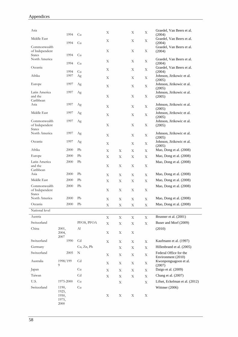
Appendices
Asia 1994 Cu X X X Graedel, Van Beers et al.
(2004) Middle East
1994 Cu X X X Graedel, Van Beers et al. (2004)
Commonwealth of Independent States 1994 Cu
X X X Graedel, Van Beers et al. (2004)
North America 1994 Cu X X X Graedel, Van Beers et al.
(2004) Oceania
1994 Cu X X X Graedel, Van Beers et al. (2004)
Afrika 1997 Ag X X X Johnson, Jirikowic et al. (2005)
Europe 1997 Ag X X X Johnson, Jirikowic et al. (2005)
Latin America and the Caribbean
1997 Ag X X X
Johnson, Jirikowic et al. (2005)
Asia 1997 Ag X X X Johnson, Jirikowic et al. (2005)
Middle East 1997 Ag X X X Johnson, Jirikowic et al. (2005)
Commonwealth of Independent States
1997 Ag X X X
Johnson, Jirikowic et al. (2005)
North America 1997 Ag X X X Johnson, Jirikowic et al. (2005)
Oceania 1997 Ag X X X Johnson, Jirikowic et al. (2005)
Afrika 2000 Pb X X X X Mao, Dong et al. (2008) Europe 2000 Pb X X X X Mao, Dong et al. (2008) Latin America and the Caribbean
2000 Pb X X X X
Mao, Dong et al. (2008)
Asia 2000 Pb X X X X Mao, Dong et al. (2008) Middle East 2000 Pb X X X X Mao, Dong et al. (2008) Commonwealth of Independent States
2000 Pb X X X X
Mao, Dong et al. (2008)
North America 2000 Pb X X X X Mao, Dong et al. (2008) Oceania 2000 Pb X X X X Mao, Dong et al. (2008)
National level
Austria X X X X Brunner et al. (2001) Switzerland PFOS, PFOA X X X X Buser and Morf (2009) China 2001,
2004, 2007
Al X X X
(2010)
Switzerland 1990 Cd X X X X Kaufmann et al. (1997) Germany Cu, Zn, Pb X X X Hillenbrand et al. (2005) Switzerland 2005 N X X X X Federal Office for the
Environment (2010) Australia 1998/199
9 Cd X X X X Kwonpongsagoon et al.
(2007) Japan Cu X X X X Daigo et al. (2009) Taiwan Cd X X X X Chang et al. (2007) U.S. 1975-2000 Cu X X Lifset, Eckelman et al. (2012) Switzerland 1190,
1925, 1950, 1975, 2000
Cu
X X X X
Wittmer (2006)
58

Appendices
Austria 2003 Fe, Cu, Zn, Al X X Döberl et al. (2004) China 1994, 200,
2004 Cu, Zn, Ni X X X X Wang et al. (2008)
Austria FCKW X X X X Obernosterer et al. (2005) Austria 2001 N X X X X Obernosterer et al. (2003) Austria 1994 Zn X X X X Daxbeck et al. (1998) Norway n.a. Cd X Mykeelbost et al. (1997) Norway n.a. DEHP X Mykeelbost and Rypdal
(1997) Switzerland Sb X X X X Mathys et al. (2007) Taiwan Zn X Ma et al. (2011) Switzerland 1980-2020 DecaBDE,
HBCD, BDE-27
X X X X Morf et al. (2007)
Austria n.a. Estron, 17-β-Estradiol, Estriol, Ethinylestradiol (EE2), Bisphe-nol A und Nonylphenol
X X X X
Skutan et al. (2003)
Brazil 2005 Cu X X X Tanimoto et al. (2010) Germany Ga, In, Mn, Ni,
Pa, Ag, Ti, Zn, Sn
X X X X Wittmer, Erren et al. (2011), Wittmer et al. (2011)
Austria 2001 Al X X Pilz et al. (2003) Austria 2003 Cu X X X X Daxbeck et al. (2006) India 2010 Ag X X X X Burger Chakraborty, Qureshi
et al. (2013) Netherland 1990 Cd, Cu, Pb, Zn X X X X Guinée, van den Bergh et al.
(1999) Peru 1997 Ag X X X Johnson, Jirikowic et al.
(2005) United States 1997 Ag X X X Johnson, Jirikowic et al.
(2005) Mexico 1997 Ag X X X Johnson, Jirikowic et al.
(2005) France 1997 Ag X X X Johnson, Jirikowic et al.
(2005) India 1997 Ag X X X Johnson, Jirikowic et al.
(2005) Germany 1997 Ag X X X Johnson, Jirikowic et al.
(2005) Zambia 1994 Cu X X X Graedel, Van Beers et al.
(2004) Germany 1994 Cu X X X Graedel, Van Beers et al.
(2004) Saudi Arabia 1994 Cu X X X Graedel, Van Beers et al.
(2004) China 1994 Cu X X X Graedel, Van Beers et al.
(2004) United States 2000 Pb X X X X Mao, Dong et al. (2008) France 2000 Pb X X X X Mao, Dong et al. (2008) United Kingdom
2000 Pb X X X X Mao, Dong et al. (2008)
Italy 2000 Pb X X X X Mao, Dong et al. (2008) Japan 2000 Pb X X X X Mao, Dong et al. (2008) India 2000 Pb X X X X Mao, Dong et al. (2008)
Regional level
59

Appendices
Minnesota 1990, 2000, 2005
Hg X X X X
Barr Engineering Company (2001)
Unteres Bünztal 1986/1987
N, P, Cl, Cu, Zn, Cd, Pb (waterborne)
X X Henseler et al. (1992)
Sundgau region (CH)
n.a. P, Cd, Zn, X X X Keller et al. (2001)
Upper Parramata river catchment (Australia)
2004-2005 Cu (waterborne) X X X
Seelsaen (2007)
Rural region in Lower Austria
n.a. N, P (waterborne) X Zessner et al. (2002)
Rural region in Lower Austria
n.a. Zn, Cu, Pb, Cd (waterborne) X Zessner and Lampert (2002)
Swedish municipalities
1995, 1998
Cd X X X Lindqvist et al. (2004)
Rhine River Mid 1960, 1988
Cd, Zn, Pb X X Stigliani et al. (1993)
Hudson River basin
Heavy metal, pesticides and herbicides, other critical pollutants
X X
Ayres et al. (1986)
Los Angeles Basin
1972 Pb X X Huntzicker et al. (1975)
Generic region n.a. DEHP (waterborne) X X X X De Keyser et al. (2010)
City level Stockholm 1995 Cd, Cr, Cu, Pb,
Hg, Ni, Zn X X X X Bergbäck et al. (2001)
Vienna 1991 N, C, Pb X X X X Daxbeck et al. (1996) Bangkok 1996 N, P X X X Færge et al. (2001) Stockholm 1900-1995 Ce, Cr, Cu, Pb,
Hg, Zn X X X X Hedbrant (2001)
Stockholm 1995 Cu, Zn, Cd, Pb (waterborne) X X X X Jonsson (2000)
Stockholm 2002, 2004, 2005
DEHP, APEO, PBDE, CP X X
Jonsson et al. (2008)
Vienna n.a. Al, Cu, Pb, X X Obernosterer et al. (2003) Stockholm Pb, Zn X X Palm and Ostlund (1996) Villach Pb, Cd, Zn, Cu
(waterborne) X X X Rebernig (2007)
Stockholm Cd, Cr, Cu, Hg, Ni, Pb, Zn X Sörme et al. (2001)
Sydney 2000 P X X X X Tangsubkul et al. (2005) Chaohu City 2008 P X X X X Yuan et al. (2011) Vienna 2010 c-PentaBDE,
c-OctaBDE X X X X Vyzinkarova et al. (2013)
Greater Toronto Area
2005 C X X X X Mohareb and Kennedy (2012)
Gothenburg 2009 P X X X X Kalmykova et al. (2012) Paris 1801-1914 N X X Barles (2007) Paris 2006 N X X X X Svirejeva-Hopkins et al.
(2011) Nhat Tan, Hoang Tay (Vietnam)
2008 N, P X X X X
Do-Thu et al. (2011)
Note: n.a. = not available
60

Appendices
REFERENCES
Ayres, R. U. and S. R. Rod. 1986. Patterns of pollution in the Hudson-Raritan basin. Environment 28(4): 14-20, 39-43. Barles, S. 2007. Feeding the city: Food consumption and flow of nitrogen, Paris, 1801–1914. Science of The Total Environment 375(1–3): 48-58. Barr Engineering Company. 2001. Substance Flow Analysis of Mercury in Products. Minneapolis, MN: Barr Engineering Company. Bergbäck, B., K. Johansson and U. Mohlander. 2001. Urban Metal Flows – A Case Study of Stockholm. Review and Conclusions. Water, Air, and Soil Pollution: Focus 1(3): 3-24. Bertram, M., M. Hryniuk, G. Kirchner, et al. 2006. Aluminium Recycling in Europe. Brussels: European Aluminium Association (EAA). Brunner, P. H., G. Döberl, M. Eder, et al. 2001. Bewertung abfallwirtschaftlicher Maßnahmen mit dem Ziel der nachsorgefreien Deponie. [Assessment of measures in the waste system with respect to aftercare-free landfills.] Wien: Umweltbundesamt. Burger Chakraborty, L., A. Qureshi, C. Vadenbo, et al. 2013. Anthropogenic mercury flows in India and impacts of emission controls. Environ Sci Technol 47(15): 8105-8113. Buser, A. and L. S. Morf. 2009. Substance flow analysis for Switzerland: Perfluorinated surfactants perfluorooctanesulfonate (PFOS) and perfluorooctanoic acid (PFOA). Bern: Federal Office for the Environment. Chang, I. C., T.-Y. Hsiao, Y.-H. Yu, et al. 2007. Identification of Pollution Source of Cadmium in Soil. Application of Material Flow Analysis and A Case Study in Taiwan. Environmental Science and Pollution Research 14(1): 49-59. Chen, W. Q., L. Shi and Y. Qian. 2010. Substance flow analysis of aluminium in mainland China for 2001, 2004 and 2007: Exploring its initial sources, eventual sinks and the pathways linking them. Resources Conservation and Recycling 54(9): 557-570. Daigo, I., S. Hashimoto, Y. Matsuno, et al. 2009. Material stocks and flows accounting for copper and copper-based alloys in Japan. Resources, Conservation and Recycling 53(4): 208-217. Daxbeck, H., C. Lampert, L. S. Morf, et al. 1996. Der anthropogene Stoffhaushalt der Stadt Wien - N, C und Pb. [The anthropogenic metabolism of Vienna - Nitrogen, Carbon and Lead.] Wien: Technische Universität Wien. Daxbeck, H., A. Schönbauer and P. H. Brunner. 1998. Machbarkeitsstudie Nationale Stoffbuchhaltung. Testbeispiel Zink. [Feasibility study National Substance Accounting. Case study zinc.] Wien: Umweltbundesamt. Daxbeck, H., M. Stockinger and B. Brand. 2006. Beitrag der Abfallwirtschaft zum Kupferhaushalt Österreich. [Role of waste management in the Austrian copper metabolism.] Wien: Ressourcen Management Agentur. De Keyser, W., V. Gevaert, F. Verdonck, et al. 2010. Combining multimedia models with integrated urban water system models for micropollutants. Water Sci Technol 62(7): 1614-1622.
61

Appendices
Do-Thu, N., A. Morel, H. Nguyen-Viet, et al. 2011. Assessing nutrient fluxes in a Vietnamese rural area despite limited and highly uncertain data. Resources, Conservation and Recycling 55(9-10): 849-856. Döberl, G., R. Fehringer, B. Müller, et al. 2004. Verknüpfung Rohstofflager - anthropogene Lager - letzte Senken. [Linking primary resource stocks, anthropogenic stocks and final sinks.] Wien: Bundesministerium für Wirtschaft und Arbeit. Eckelman, M. J. and T. E. Graedel. 2007. Silver Emissions and their Environmental Impacts: A Multilevel Assessment. Environmental Science & Technology 41(17): 6283-6289. Færge, J., J. Magid and F. W. T. Penning De Vries. 2001. Urban nutrient balance for Bangkok. Ecological Modelling 139(1): 63-74. Federal Office for the Environment. 2010. Nitrogen fluxes in Switzerland. Bern: Federal Office for the Environment (FOEN). Graedel, T., D. Van Beers, M. Bertram, et al. 2004. Multilevel cycle of anthropogenic copper. Environmental Science & Technology 38(4): 1242-1252. Guinée, J. B., J. C. J. M. van den Bergh, J. Boelens, et al. 1999. Evaluation of risks of metal flows and accumulation in economy and environment. Ecological Economics 30(1): 47-65. Hedbrant, J. 2001. Stockhome: A Spreadsheet Model of Urban Heavy Metal Metabolism. Water, Air, & Soil Pollution: Focus 1(3): 55-66. Henseler, G., R. Scheidegger and P. H. Brunner. 1992. Die Bestimmung von Stoffflüssen im Wasserhaushalt einer Region. [Determination of Material Flux through the Hydrosphere of a Region.] Vom Wasser 78: 91-116. Hillenbrand, T., D. Toussaint, E. Böhm, et al. 2005. Einträge von Kupfer, Zink und Blei in Gewässer und Böden - Analyse der Emissionspfade und möglicher Emissionsminderungsmaßnahmen. [Discharges of copper, zinc and lead to water and soil - analysis of the emission pathways and possible emission reduction measures.] Dessau: Umweltbundesamt. Huntzicker, J. J., S. K. Friedlander and C. I. Davidson. 1975. Material balance for automobile-emitted lead in Los Angeles basin. Environmental Science & Technology 9(5): 448-457. ICdA. 2013. Cadmium emissions. The International Cadmium Association (ICdA). Retrieved 24th September 2013, from www.cadmium.org. Izard, C. F. and D. B. Müller. 2010. Tracking the devil's metal: Historical global and contemporary U.S. tin cycles. Resources, Conservation and Recycling 54(12): 1436-1441. Johnson, J., J. Jirikowic, M. Bertram, et al. 2005. Contemporary anthropogenic silver cycle: a multilevel analysis. Environ Sci Technol 39(12): 4655-4665. Jonsson, A. 2000. The Trace of Metals - Use, Emissions and sediment load of urban heavy metals. PhD Thesis, Linköping: Linköping University. Jonsson, A., U. Fridén, K. Thuresson, et al. 2008. Substance Flow Analyses of Organic Pollutants in Stockholm. Water, Air, & Soil Pollution: Focus 8(5): 433-443.
62

Appendices
Kalmykova, Y., R. Harder, H. Borgestedt, et al. 2012. Pathways and Management of Phosphorus in Urban Areas. Journal of Industrial Ecology 16(6): 928-939. Kaufmann, M., C. v. Schulthess and M. Ziegler. 1997. Cadmium - Stoffflussanalyse. [Cadmium - Substance flow analysis.] Bern: Bundesamt für Umwelt Wald und Landschaft. Keller, A., B. von Steiger, S. E. A. T. M. van der Zee, et al. 2001. A Stochastic Empirical Model for Regional Heavy-Metal Balances in Agroecosystems. J. Environ. Qual. 30(6): 1976-1989. Kwonpongsagoon, S., H. P. Bader and R. Scheidegger. 2007. Modelling cadmium flows in Australia on the basis of a substance flow analysis. Clean Techn Environ Policy 9. Lifset, R. J., M. J. Eckelman, E. M. Harper, et al. 2012. Metal lost and found: dissipative uses and releases of copper in the United States 1975-2000. Sci Total Environ 417-418(0): 138-147. Lindqvist, A. and F. von Malmborg. 2004. What can we learn from local substance flow analyses? The review of cadmium flows in Swedish municipalities. Journal of Cleaner Production 12(8–10): 909-918. Liu, G. and D. B. Muller. 2013. Mapping the global journey of anthropogenic aluminum: a trade-linked multilevel material flow analysis. Environ Sci Technol 47(20): 11873-11881. Ma, H. W., K. Matsubae, K. Nakajima, et al. 2011. Substance flow analysis of zinc cycle and current status of electric arc furnace dust management for zinc recovery in Taiwan. Resources Conservation and Recycling 56(1): 134-140. Mao, J. S., J. Cao and T. E. Graedel. 2009. Losses to the environment from the multilevel cycle of anthropogenic lead. Environmental Pollution 157(10): 2670-2677. Mao, J. S., J. Dong and T. E. Graedel. 2008. The multilevel cycle of anthropogenic lead: II. Results and discussion. Resources, Conservation and Recycling 52(8–9): 1050-1057. Mathys, R., J. Dittmar and C. A. Johnson. 2007. Antimony in Switzerland: A substance flow analysis. Bern: Federal Office for the Environment. Mohareb, E. and C. Kennedy. 2012. Gross Direct and Embodied Carbon Sinks for Urban Inventories. Journal of Industrial Ecology 16(3): 302-316. Morf, L. S., A. Buser and R. Taverna. 2007. Endocrine Disruptors: Relevance for Humans, Animals and Ecosystems. Dynamic Substance Flow Analysis Model for Selected Brominated Flame Retardants as a Base for Decision Making on Risk Reduction Measures (FABRO). Zürich: GEO Partner AG. Mykeelbost, T. and K. Rypdal. 1997. Material flow analysis of Cadmium and di-2-ethylhexylphthalate (DEHP) in Norway. Oslo: Statistic Norway. Department of Economic Statistics. Obernosterer, R. and I. Reiner. 2003. Stickstoffbilanz Österreich. Beitrag der Abfallwirtschaft zum Stickstoffhaushalt Österreich. [Austrian Nitrogen balance. Role of the waste management sector to the nitrogen metabolism in Austria.] Villach: Ressourcen Management Agentur. Obernosterer, R., I. Reiner and R. Smutny. 2003. Urbanes Ressourcen Management: Fallstudie Wien. Teilbereich: Schadstoffmanagement diffuser Metallemissionen. [Urban Resource Management: Case Study Vienna. Subsection: Contaminant Management of diffuse metal emissions.] Wien/Villach: Ressourcen Management Agentur.
63

Appendices
Obernosterer, R., R. Smutny and E. Jäger. 2005. Nachhaltige FCKW Bewirtschaftung Österreich. [Sustainable CFC management in Austria.] Villach: Ressourcen Management Agentur. Odnevall Wallinder, I., B. Bahar, C. Leygraf, et al. 2007. Modelling and mapping of copper runoff for Europe. Journal of Environmental Monitoring 9(1): 66-73. Ott, C. and H. Rechberger. 2012. The European phosphorus balance. Resources Conservation and Recycling 60(0): 159-172. Pacyna, E. G., J. M. Pacyna, J. Fudala, et al. 2007. Current and future emissions of selected heavy metals to the atmosphere from anthropogenic sources in Europe. Atmospheric Environment 41(38): 8557-8566. Pacyna, J. M. 2009. Material Flow Analysis for selected Priority Substances. Oslo: Norwegian Institute for Air Research (NILU). Palm, V. and C. Ostlund. 1996. Lead and zinc flows from technosphere to biosphere in a city region. Science of the Total Environment 192(1): 95-109. Pilz, H., E. Kletzer and F. Neubacher. 2003. Beitrag der Abfallwirtschaft zum Aluminiumhaushalt Österreich. [Role of the waste management sector for the Austrian aluminum metabolism.] Wien: Gesellschaft für umfassende Analysen. Rebernig, G. 2007. Methode zur Analyse und Bewertung der Stoffflüsse von Oberflächen einer Stadt. [A method to analyse and evaluate substance flows resulting from urban surfaces.] PhD Thesis, Wien: Technische Universität Wien. Reck, B. and R. Gordon. 2008. Nickel and chromium cycles: Stocks and flows project part IV. JOM 60(7): 55-59. Seelsaen, N. 2007. Development of an integrated approach to understanding, managing and designing strategies and recycled organics filtration treatment system to control regional heavy metal contamination of stormwater. PhD Thesis, Sydney: The University of New South Wales. Skutan, S. and P. H. Brunner. 2003. Stoffflußanalyse ausgewählter endokrin wirksamer Substanzen (interner Endbericht). [Substance flow analysis of selected endocrine disruptors (internal report).] Wien: Technische Universität Wien. Sörme, L., B. Bergbäck and U. Lohm. 2001. Century Perspective of Heavy Metal Use in Urban Areas. A Case Study in Stockholm. Water, Air and Soil Pollution: Focus 1(3-4): 197-211. Stigliani, W. M., P. R. Jaffé and S. Anderberg. 1993. Heavy metal pollution in the Rhine Basin. Environmental Science and Technology 27(5): 786-793. Sundseth, K., J. Pacyna, E. Pacyna, et al. 2012. Substance Flow Analysis of Mercury Affecting Water Quality in the European Union. Water, Air, & Soil Pollution 223(1): 429-442. Svirejeva-Hopkins, A., S. Reis, J. Magid, et al. 2011. Nitrogen flows and fate in urban landscapes. In The European Nitrogen Assessment, edited by M. A. Sutton, C. M. Howard, J. W. Erisman et al. Cambridge: Cambridge University Press. Tangsubkul, N., S. Moore and T. D. Waite. 2005. Incorporating phosphorus management considerations into wastewater management practice. Environmental Science & Policy 8(1): 1-15.
64

Appendices
Tanimoto, A. H., X. Gabarrell Durany, G. Villalba, et al. 2010. Material flow accounting of the copper cycle in Brazil. Resources, Conservation and Recycling 55(1): 20-28. Vyzinkarova, D. and P. H. Brunner. 2013. Substance Flow Analysis of Wastes Containing Polybrominated Diphenyl Ethers. Journal of Industrial Ecology 17(6): 900-911. Wang, T., J. Mao, J. Johnson, et al. 2008. Anthropogenic metal cycles in China. Journal of Material Cycles and Waste Management 10(2): 188-197. Wittmer, D. 2006. Kupfer im regionalen Ressourcenhaushalt - Ein methodischer Beitrag zur Exploration urbaner Lagerstätten. [Copper in the regional metabolism - a methodological contribution for explorating urban resource stocks.] PhD Thesis, Zürich: ETH Zürich. Wittmer, D., M. Erren, C. Lauwigi, et al. 2011. Umweltrelevante metallische Rohstoffe: Meilensteinbericht des Arbeitsschrittes 2.1 des Projekts "Materialeffizienz und Ressourcenschonung" (MaRess). Teil 2, Abschlussbericht. [Environmental relevant metal resources: Final report of workpackage 2.2, project "MaRess". Part 2.] Wuppertal: Wuppertal Institut. Wittmer, D., M. Scharp, S. Bringezu, et al. 2011. Umweltrelevante metallische Rohstoffe: Meilensteinbericht des Arbeitsschrittes 2.1 des Projekts "Materialeffizienz und Ressourcenschonung" (MaRess). Teil 1, Abschlussbericht. [Environmental relevant metal resources: Final report of workpackage 2.1, project "MaRess". Part 1.] Wuppertal: Wuppertal Institut. Yuan, Z., J. Shi, H. Wu, et al. 2011. Understanding the anthropogenic phosphorus pathway with substance flow analysis at the city level. Journal of Environmental Management 92(8): 2021-2028. Zessner, M. and C. Lampert. 2002. The use of regional material balances in water quality management. Urban Water 4(1): 73-83.
65


Appendices
Appendix III: Articles The appendix III includes (1) the list of articles and their link to the thesis, (2) the statement from
co-authors regarding the permit to include the articles, (3) my contributions to each article, and (4)
the articles itself.
Included articles and link to the thesis
This thesis includes three original research articles:
I. Kral, U., Kellner, K., Brunner, P.H., 2013. Sustainable resource use requires “clean
cycles” and safe “final sinks”. Online: http://dx.doi.org/10.1016/j.scitotenv.2012.08.094.
Science of the Total Environment 461–462, 819-822.
II. Kral, U., Lin, C.Y., Kellner, K., Ma, H.-W., Brunner, P.H., 2014. The copper balance of
cities: Exploratory insights into a European and an Asian city. Journal of Industrial
Ecology. Online: http://dx.doi.org/10.1111/jiec.12088. In press.
III. Kral, U., Brunner, P.H, Chen, P.C., Chen, S.R.. Sinks as limited resources? - A new
indicator for evaluating anthropogenic material flows. Journal of Ecological Indicators.
Submitted on 18th January 2014, 1st revisions submitted on 16th May 2014.
Two (article I, article II) out of three articles are published in peer-reviewed, international journals.
They are available online under open access license and are included in the thesis. They are
reprinted according to the authors’ rights of the Publishers Elsevier and Wiley-Blackwell,
respectively. One (article III) out of three articles was submitted to the Journal of Ecological
Indicators on 18 January 2014, the 1st revision was submitted on 16 May, and is at present with the
editor. The article is included in appendix III in accordance with the author’s rights of the Publisher
Elsevier.
Table III-1: Included articles and link to individual chapters of the thesis
Background and problem
definition
Indicator definition and interpretation
Inventory analysis
Impact assessment
Results and discussion
chapter 1.1 chapter 3.1 chapter 3.3, 4.2 chapter 3.4, 4.3 chapter 5 Article I X X Article II X Article III X X X X
67

Appendices
Statement from Co-authors
Note: The Annex “Declaration by the candidate” can be found in the next chapter “Authors
contribution”.
68

Appendices
Authors contribution
For all three articles I have (a) reviewed the literature for contextualizing the research done, (b)
suggested article content and structure, (c) took the lead in text writing and figure creation, and (d)
handled the submission, review and editorial phase until publication. All articles are the result of
collaborative work with theoretical and empirical contributions from my side:
Table III-2: Authors contribution to article I
Task Kral, U. Kellner, K. Brunner, P.H. Initial idea about the research topic o o ++
Conception and design of the article ++ + o
Supervision n.r. n.r. ++
Notes: ++ = major contribution; + = minor contribution; o = no contribution; n.r. = not relevant
Table III-3: Authors contribution to article II
Task Kral, U. Lin, C.Y. Kellner, K. Ma, H.W. Brunner, P.H.
Model development + o + + + Data acquisition for Vienna + o ++ o o
Data acquisition for Taipei o ++ o o o
Data treatment in view of city comparison ++ + o o o
SFA indicator development + + o o +
SFA indicator quantification + + o o o
Supervision n.r. n.r. n.r. + ++
Notes: ++ = major contribution; + = minor contribution; o = no contribution; n.r. = not relevant
Table III-4: Authors contribution to article III
Task Kral, U. Brunner, P.H. Chen, P.C. Chen, S.R. Sink indicator development ++ + o o Case study “Cu Vienna” ++ o o o Case study “Pb Vienna” ++ o + + Case study “PFOS Switzerland” ++ o o o
Supervision n.r. ++ n.r. n.r.
Notes: ++ = major contribution; + = minor contribution; o = no contribution; n.r. = not relevant
69


Appended articles
Article I – Main article
………………………………… AIII-1
Article II – Main article
Article II – Supporting information
…………………………………
…………………………………
AIII-7
AIII-21
Article III – Main article
Article III – Supporting information
…………………………………
…………………………………
AIII-77
AIII-107
71


Article I
Kral, U., Kellner, K., Brunner, P.H., 2013. Sustainable resource use requires “clean cycles” and
safe “final sinks”. Online: http://dx.doi.org/10.1016/j.scitotenv.2012.08.094. Science of the Total
Environment 461–462, 819-822.
AIII-1

Sustainable resource use requires “clean cycles” and safe “final sinks”
Ulrich Kral ⁎, Katharina Kellner, Paul H. BrunnerInstitute for Water Quality, Resource and Waste Management, Vienna University of Technology, Karlsplatz 13/226, 1040 Vienna, Austria
H I G H L I G H T S
► Present recycling policies focus toomuch on maximizing recycling rates.
► Hazardous materials are kept in cyclesinstead of eliminating them from cy-cles.
► New priorities must be set to establishclean cycles.
► A clean cycle strategy results in resi-dues that must be disposed of insinks.
► Waste management must supply suit-able sinks for substances eliminatedfrom cycles.
G R A P H I C A L A B S T R A C T
a b s t r a c ta r t i c l e i n f o
Article history:Received 10 July 2012Received in revised form 14 August 2012Accepted 27 August 2012Available online 25 September 2012
Guest Editors: Christian Ludwig,Xaver Edelmann, Martin Lehmann
Keywords:Clean cycleFinal sinkSubstance flow analysisRecycling strategyWaste management
In order to fulfill the objectives of environmental protection, today's focus on quantitative recycling ratesmust be amended by a more qualitative approach. Because modern products represent a mix of numerousand sometimes hazardous substances, ways must be explored to remove detrimental substances duringrecycling and to establish “clean cycles”. On the one hand, such a “clean cycle” strategy will result in betterrecycling qualities of secondary products and less dissipation of hazardous substances during further productuse. On the other hand, the elimination of hazardous substances during recycling requires sinks for the dis-posal of the eliminated materials. These topics are presented in general as well as by case studies. In partic-ular, the sink issue is addressed, differentiating between sinks and final sinks and discussing the challenge tosupply appropriate final sinks for all materials that cannot be recycled.
© 2012 Elsevier B.V. All rights reserved.
1. Introduction
Ona global scale, there's a continuous increase ofmaterial extractionfrom the earth's crust (Weber et al., 2011), resulting in large accumula-tions of materials particularly in urban areas. While the anthropogenicmaterial stocks are growing, the amount of waste flows and emissionrates increase with a certain delay. To satisfy contemporary resource
needs and to decrease environmental loadings, an obvious solution isto recycle as much as possible in order to substitute primary resources.Therefore, European legislation aims to increase recycling rates contin-uously. This quantitative approach does not take into account thepresence of unwanted substances ending up in the second generationproducts. To avoid this, a so called “clean cycle” strategy is proposed.
2. “Clean cycle” strategy
Sustainable resource use is characterized by an ecologically ac-ceptable impact on nature. Recycling strategies play a key role by
Science of the Total Environment 461–462 (2013) 819–822
⁎ Corresponding author.E-mail addresses: [email protected] (U. Kral), [email protected]
(K. Kellner), [email protected] (P.H. Brunner).
0048-9697/$ – see front matter © 2012 Elsevier B.V. All rights reserved.http://dx.doi.org/10.1016/j.scitotenv.2012.08.094
Contents lists available at SciVerse ScienceDirect
Science of the Total Environment
j ourna l homepage: www.e lsev ie r .com/ locate /sc i totenv
AIII-2

extending materials' lifespan and reducing environmental impacts.Until now, the focus of environmental evaluation methodologies hasbeen laid on emission rates, the composition of second life productshas only rarely been considered in view of hazardous constituents,multiple recycling loops, and long term effects. There is no focus yeton the fact that today's recycling loops contain valuable as well asharmful substances. Even though cycling of hazardous substances isprohibited by waste management directives (Republik Österreich,2008), the recycling quota regulation as well as economic constraintsresult in hazardous substances to remain in cycles. Hence, “tramp el-ements” accumulate in the anthroposphere with potential negativeeffects on a) product quality, and b) environment:
ad a) Some “tramp elements” accumulate finely dispersed in the prod-uct cycle and lower the quality of second generation goods madeup from secondary resources. This becomes apparent for exam-ple in the plastic industry, where stabilizers like cadmium, leadand tin contaminate the recycling products (Fehringer et al.,1997), or in the steel industry, where copper contaminates thesteel cycle (Gleich et al., 2004), or in packaging industry, wheremineral oils contaminate paperboards used for food packaging(Kappen et al., 2012). In short, the goals of high recycling ratesand high product qualities often contradict each other.
ad b) The accumulation of toxic “tramp elements” in the product cyclepresents an increasing potential for the release of hazardoussubstances. The reason is that some fractions of a material are in-evitable released throughout the entire life cycle (see Fig. 1). Inother words, substances from the stock-in-use are convertedinto unrecoverable forms and dissipated into the environment(Ayres et al., 2002). For example, in 1983 about 10%–30% of re-fined copper left the product cycle and ended up in environmentor landfills (Bureau of Mines, 1983; Nriagu and Pacyna, 1988).Exemplary, emission sources are roofs and brake wear. Theproducts are exposed to abrasion, corrosion andweathering pro-cesses which effect dissipative material releases. The great ma-jority of these dissipated materials accumulate in specificenvironmental compartments and may threaten to impact natu-ral processes (Geiser, 2001). A case study on urban surfacesshows that about 1/3 of the diffusively emitted copper entersthe waste management system. In contrast, roughly 2/3 is di-rectly lost in an uncontrolled form to the environment(Rebernig, 2007). While the scientific community is increasinglyaware of these kinds of material losses (e.g. Arx, 2006; Bergbäcket al., 2001; Burkhardt et al., 2007, 2008; Obernosterer et al.,
2003; Sörme et al., 2001), few guidelines were developed tokeep dissipative losses from urban surfaces and abrasion onlow levels (Hoffmann and Rudolphi, 2005; Zysset et al., 2002).In the future, dissipative material losses from all sources andtheir effects on the environment must be taken into account todetermine sustainable resource use.
In order to establish a sustainable resource use with no burden forfuture generations, hazardous substances have to be eliminated frommaterial cycles. Otherwise recycling strategies run the risk to a) sup-port a qualitative down-cycling of materials in a large scale format,and b) raise the potential for harmful material losses throughoutthe material life cycle.
There are two conclusions regarding a sustainable recycling policywhich incorporates a “clean cycle” strategy:
• For environmental protection and product quality reasons, therecycling quotes have to take qualitative characteristics regardingsecondary materials into account. The dilution of unwanted sub-stances in second generation products as well as the total release ofharmful substances to the environment has to be taken under control.
• If “clean cycles” are established, the safe disposal of specific sub-stances removed from the cycles is mandatory. These contaminatedmaterial flows have to enter safe “final sinks”. Consequently, a safe“final sink” concept with corresponding policy instruments has tobe developed.
Fig. 2 displays the resulting material flows based on a “clean cycle”strategy. An optimum mix of primary and clean secondary materialkeeps the material cycle alive. Impurities and dissipative materiallosses are directed to safe final sinks.
3. The need for final sinks
In 1965 Albert Wolman was the first who analyzed cities as meta-bolic systems (Wolman, 1965). He highlighted the fact, that materialuse is directly linked with emissions and waste. The discussion aboutthe need for sinks to take up substance flows became public aware-ness in 1987, where the Brundtland report states the importance of“ultimate sinks for the by-products of human activities” (UnitedNations, 1987). In 1996, Joel Tarr – an environmental historian –
has drawn the attention to “the search of the ultimate sink” from ahistorical perspective (Tarr, 1996). At the same time Marina Albertihighlighted the fact that “cities cannot sustain themselves withoutdrawing on the carrying capacity of their hinterland or region at the
Fig. 1. Anthropogenic material stocks and flows.
820 U. Kral et al. / Science of the Total Environment 461–462 (2013) 819–822
AIII-3

back end of their metabolism” (Alberti, 1996). Now it's time to devel-op a systematic “sink concept” that links urban output flows withmanmade or natural sinks. The definition of sink indicators can alsosupport the evaluation of ecological sustainability (Döberl andBrunner, 2004), and thus contribute to the reduction of the risk ofoverloading sinks, such as today's excessive flow of greenhousegases to the sink “atmosphere” (Brunner, 2010).
From a materials management point of view, the anthropospherecan be seen as flow through reactor with a distinctive storage function.Material flows leave the anthropogenic material cycle (see Fig. 2), dueto a) the second law of thermodynamics (dissipative losses occur)and, b) the diminishing returns (secondary resources). The core ques-tion is: Where should these off-flows end up? The answer on a generallevel is: They have to end up in final sinks. A more concrete answer re-mains to be developed because at present, the sink concept is still avague framework. Based on previous definitions, the authors put thefollowing working hypothesis forward for discussion:
• A “sink” is defined as a process that receives anthropogenic materialflows that have no positive value for present societies.
• A “final sink” is a sink that either destroys a substance completely,or that holds a substance for a very long time period.
In order to exemplify the term “sink” and “final sink”, two casestudies are discussed. They focus on: a) the retention in the environ-ment of anthropogenic materials that have been previously lost bydissipation, and b) the elimination of copper from the steel cycleand the deposit of recycling residues.
ad a) Glaciers act as receptor for a broad range of dissipative, air-borne losses like heavy metals or persistent organic pollutants(POPs). Thus glacier ice is a “sink” that can become a secondarysource of pollutants (Salomons, 1998). Recently, a Swiss study(Bogdal et al., 2009) identified an accelerated release of pollut-ants from melting Alpine glaciers. This might result in an
accumulation of hazardous substances in the food chain up tofishes or plants growing in glacier water. The case study exem-plifies the term sink as used here for the temporary storageprocess “glacier ice”, and reveals that so far many anthropo-genic flows of hazardous substances have not yet reached anenvironmentally safe “final sink”.
ad b) Due to technological constraints, it is difficult and costly to re-move copper during steel recycling. So, traces of copper remainand accumulate in the product cycle. This results in down cy-cling and lower product quality. In order to achieve appropri-ate product qualities, steel companies select scrap fractionson the resource market depending on the copper concentra-tion. A study about sustainable metal management (Gleich etal., 2004) indicates, that in the future, copper concentrationswill become so high that specific scrap fractions cannot beused as secondary resource in the steel industry anymore. Sce-narios were identified as reasonable that remove part of thescrap from the recycling stream in order to dispose them offin manmade sinks like landfills.
The example shows that a) steel is a temporary sink for copperand the steel cycle eventually stresses long term sinks like landfills,and b) the selection of scrap depends on quality criteria. So, steelrecycling quotes are quality driven and can't be achieved by pre-scribed recycling rates. The exclusive definition of recycling rates ona quantitative base blinds out the qualitative constraints of recycling.In order to guarantee a clean steel cycle, recycling policies have toconsider product qualities too.
Concluding, both the whole range of dissipative material losses1
and impurities within products have to be directed to safe finalsinks. If a safe final sink can't be identified for ecological, technical
1 Dissipative material losses cover point and diffuse emissions with no option forrecovery.
Fig. 2. Material flows based on a “clean cycle” strategy (Stumm and Davis, 1974, modified).
821U. Kral et al. / Science of the Total Environment 461–462 (2013) 819–822
AIII-4

or economic reasons, material design strategies have to be developedthat consider final sink limitations, such as in the case of fossil fuelswhere a safe mediate term sink for carbon is missing.
4. Conclusion
In order to achieve sustainable resource management, a strategydirected towards clean cycles and safe final sinks needs to be devel-oped. A clean cycle strategy delivers an optimum instead of a maxi-mum of secondary resources through elimination of hazardoussubstances from material cycles. This ensures the generation of qual-ity proven recyclables for multiple life cycles of products without therisk to shift problems into the future. Removing hazardous substancesfrom material cycles requires final sinks where these substances canbe stored safely for geological time periods.
Acknowledgments
The authors gratefully acknowledge the funding by the AustrianScience Fund (FWF): I 549-N21.
References
Alberti M. Measuring urban sustainability. Environ Impact Assess Rev 1996;16:381–424.
Ayres RU, Ayres LW, Råde I. The life cycle of copper, its co-products and by-products.International Institute for Environment and Development (IIED) and World Busi-ness Council for Sustainable Development (WBCSD); 2002.
Bergbäck B, Johansson K, Mohlander U. Urban metal flows—a case study of Stockholm.Review and conclusions. Water Air Soil Pollut Focus 2001;1:3-24.
Bogdal C, Schmid P, Zennegg M, Anselmetti FS, Scheringer M, Hungerbühler K. Blastfrom the past: melting glaciers as a relevant source for persistent organic pollut-ants. Environ Sci Technol 2009;43:8173–7.
Brunner PH. Clean cycles and safe final sinks. Waste Manag Res 2010;28:575–6.Bureau of Mines. Minerals yearbook metals and minerals 1983. Washington: U.S. Bureau
of Mines; 1983.Burkhardt M, Kupper T, Hean S, Haag R, Schmid P, Kohler M, et al. Biocides used in
building materials and their leaching behavior to sewer systems. Water Sci Technol2007;56:63–7.
Burkhardt M, Rossi L, Boller M. Diffuse release of environmental hazards by railways.Desalination 2008;226:106–13.
Döberl G, Brunner PH. Substances and their (final) sinks—a new indicator for monitor-ing sustainability. Indicators for evaluating sustainable development—the ecologi-cal dimension, Berlin; 2004.
Fehringer R, Brunner PH, Baumann H. Kunststoffflüsse und Möglichkeiten derKunstoffverwendung in Österreich (in German: Plastic Flows and Possibilities forPlastic Utilization in Austria). Vienna: Vienna University of Technology; 1997.
Geiser K. Materials matter: toward a sustainable materials policy. Cambridge (Massa-chusetts), London (England): The MIT Press; 2001.
Gleich A, Brahmer-Lohss M, Gottschick M, Jepsen D, Sander K. NachhaltigeMetallwirtschaft Hamburg (in German: Sustainable Metal Management Hamburg),Hamburg; 2004.
Hoffmann M, Rudolphi A. Leitfaden für das Bauwesen—Reduktion vonSchwermetalleinträgen aus dem Bauwesen in die Umwelt (in German: Guide-lines for civil engineering—reduction of heavy metals from civil engineering toenvironment). Dessau: Environment Agency Germany; 2005.
Kappen J, Seidemann C, Demel I, Schiefer M. Sustainable paper recycling—threats,needs and future opportunities. RiskCycle Confererence—Risk-Based Managementof Chemicals and Products in a Circular Economy at Global Scale, Dresden; 2012.
Arx U. Kupfer: Verbrauch, Umwelteinträge und -vorkommen (in German: Copper:consumption, environmental impacts and availability). Umwelt-Wissen Nr. 0601.Bern: Bundesamt für Umwelt; 2006.
Nriagu JO, Pacyna JM. Quantitative assessment of worldwide contamination of air,water and soils by trace metals. Nature 1988;333:134–9.
Obernosterer R, Reiner I, Smutny R. Urbanes Ressourcen Management: Fallstudie Wien.Teilbereich: Schadstoffmanagement diffuser Metallemissionen (in German: Urbanresource management: case study Vienna. Subsection: Contaminant managementof diffuse metal emissions). Wien/Villach: Ressourcen Management Agentur(RMA); 2003.
Rebernig G. Methode zur Analyse und Bewertung der Stoffflüsse von Oberflächen einerStadt—Dissertation (in German: A method to analyse and evaluate substance flowsfrom city surface—doctoral thesis). Institut for Water Quality, Resource and WasteManagement. Vienna University of Technology, Vienna, 2007, pp. 233.
Republik Österreich. Bundesgesetz über eine nachhaltige Abfallwirtschaft(Abfallwirtschaftsgesetz 2002—AWG 2002). BGBl. I Nr. 102 (in German: AustrianWaste Management Directive 2002); 2008.
Salomons W. Biogeodynamics of contaminated sediments and soils: perspectives forfuture research. J Geochem Explor 1998;62:37–40.
Sörme L, Bergbäck B, Lohm U. Goods in the anthroposphere as a metal emission sourcea case study of Stockholm, Sweden. Water Air Soil Pollut Focus 2001;1:213–27.
Stumm W, Davis J. Kann Recycling die Umweltbeeinträchtigung vermindern? (in German:Does Recycling minimize environmental impacts?). Recycling: Lösung derUmweltkrise? (in German: Recyling: Solution of Environmental Crisis?); 1974. p. 29–41.
Tarr JA. The search for the ultimate sink: urban pollution in historical perspective.Akron: The University of Akron Press; 1996.
United Nations. Report of the World Commission on Environment and Development“Our Common Future” (Brundtland Report), Oslo; 1987.
Weber L, Zsak L, Reichl C, Schatz M. World mining data 2011. 26. Vienna: Federal Min-istry of Economy, Family and Youth; 2011.
Wolman A. The metabolism of cities. Scientific American; 1965. 213/1965.Zysset A, Hugi C, Pfammater R. Gewässerschutz bei der Entwässerung von Verkehrswegen
(in German: Traffic Runoff and Water Protection). Vollzug Umwelt. Bern: Bundesamtfür Umwelt, Wald und Landschaft (BUWAL); 2002.
822 U. Kral et al. / Science of the Total Environment 461–462 (2013) 819–822
AIII-5


Article II
Kral, U., Lin, C.Y., Kellner, K., Ma, H.-W., Brunner, P.H., 2014. The copper balance of cities:
Exploratory insights into a European and an Asian city. Journal of Industrial Ecology. Online:
http://dx.doi.org/10.1111/jiec.12088. In press.
AIII-7

R E S E A R C H A N D A N A LYS I S
The Copper Balance of CitiesExploratory Insights into a European and an Asian City
Ulrich Kral, Chih-Yi Lin, Katharina Kellner, Hwong-wen Ma, and Paul H. Brunner
Summary
Material management faces a dual challenge: on the one hand satisfying large and increasingdemands for goods and on the other hand accommodating wastes and emissions in sinks.Hence, the characterization of material flows and stocks is relevant for both improvingresource efficiency and environmental protection. This article focuses on the urban scale,a dimension rarely investigated in past metal flow studies. We compare the copper (Cu)metabolism of two cities in different economic states, namely, Vienna (Europe) and Taipei(Asia). Substance flow analysis is used to calculate urban Cu balances in a comprehensiveand transparent form. The main difference between Cu in the two cities appears to be thestock: Vienna seems close to saturation with 180 kilograms per capita (kg/cap) and a growthrate of 2% per year. In contrast, the Taipei stock of 30 kg/cap grows rapidly by 26% peryear. Even though most Cu is recycled in both cities, bottom ash from municipal solid wasteincineration represents an unused Cu potential accounting for 1% to 5% of annual demand.Nonpoint emissions are predominant; up to 50% of the loadings into the sewer system arefrom nonpoint sources. The results of this research are instrumental for the design of theCu metabolism in each city. The outcomes serve as a base for identification and recoveryof recyclables as well as for directing nonrecyclables to appropriate sinks, avoiding sensitiveenvironmental pathways. The methodology applied is well suited for city benchmarking ifsufficient data are available.
Keywords:
citiesenvironmental protectionindustrial ecologyresource efficiencysubstance flow analysis (SFA)urban metabolism
Supporting information is availableon the JIE Web site
Introduction
One of the main tasks of managing human settlements dur-ing the past 10,000 years of urban history was the sufficientsupply and disposal of materials. Driven by technology and so-cioeconomic factors, the interaction of humans with naturalresources and the environment has been in continuous changeover the years (Agudelo-Vera et al. 2011). Key developments ofthe past were the rise of cities and empires after 3000 B.C. andthe start of the industrial revolution in the eighteenth century.Global population has been increasing and resource-intensivelifestyles became predominant in the modern world. One of thepioneers who recognized the consequences of ongoing urban-ization at an early stage was Patrick Geddes (Geddes 1885). At
Address correspondence to: Ulrich Kral, Vienna University of Technology, Institute for Water Quality, Resource and Waste Management, Karlsplatz 13/226, A-1040 Vienna,Austria. Email: [email protected], Web: http://iwr.tuwien.ac.at/ressourcen
© 2014 The Authors. Journal of Industrial Ecology, published by Wiley Periodicals, Inc., on behalf of Yale University. This is an open access article under the terms of theCreative Commons Attribution License, which permits use, distribution and reproduction in any medium, provided the original work is properly cited.DOI: 10.1111/jiec.12088 Editor managing review: Seiji Hashimoto
Volume 00, Number 0
the transition from the nineteenth to the twentieth century, hecreated awareness for the massive flows of resources in cities.By pointing out material losses in the production chain throughinput-output (I/O) balancing of material budgets, he was a fore-runner of today’s material flow modeler and accountants.
Since that time, several research frameworks have been de-veloped and put forward. Approaches such as material flowanalysis (MFA) (Brunner and Rechberger 2004; Baccini andBader 1996), physical I/O analysis (e.g., Nakamura and Kondo2009; Nakamura et al. 2007; Hoekstra and Van den Bergh2006), and environmental-extended I/O analysis (e.g., Her-twich and Peters 2010; Leontief and Ford 1972) are utilized toinvestigate the anthropogenic metabolism (Baccini and Brun-ner 2012). In particular, substance flow analysis (SFA) has been
www.wileyonlinelibrary.com/journal/jie Journal of Industrial Ecology 1
AIII-8
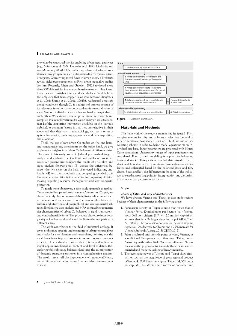
R E S E A R C H A N D A N A LYS I S
proven to be a practical tool for analyzing urban metal pathways(e.g., Mansson et al. 2009; Henseler et al. 1992; Lindqvist andvon Malmborg 2004). SFA tracks the pathway of selected sub-stances through systems such as households, enterprises, cities,or regions. Concerning metal flows in urban areas, a literaturereview yields two characteristics: First, urban metal flow studiesare rare. Recently, Chen and Graedel (2012) reviewed morethan 350 SFA articles in a comprehensive manner. They foundfive cities with insights into metal metabolism. Stockholm isthe only city that takes copper (Cu) into account (Bergbacket al. 2001; Sorme et al. 2001a, 2001b). Additional cities areunexploited even though Cu is a subject of interest because ofits relevance from both a resource and environmental point ofview. Second, individual city studies are hardly comparable toeach other. We extended the scope of literature research andcompiled 15 exemplary studies for Cu on an urban scale (see sec-tion 1 of the supporting information available on the Journal’swebsite). A common feature is that they are selective in theirscope and that they vary in methodology, such as in terms ofsystem boundaries, modeling approaches, and data acquisitionand allocation.
To fill the gap of rare urban Cu studies on the one hand,and comparative city assessments on the other hand, we giveexploratory insights into urban Cu balances of different cities.The aims of this study are to (1) develop a methodology toanalyze and evaluate the Cu flows and stocks on an urbanscale, (2) present and compare the results of a Cu flow andstock analysis for two cities, (3) discuss the differences be-tween the two cities on the basis of selected indicators, and,finally, (4) test the hypothesis that comparing metabolic dif-ferences between cities is instrumental for improving decisionmaking regarding resource management and environmentalprotection.
To reach these objectives, a case-study approach is applied.Two cities in Europe and Asia, namely, Vienna and Taipei, arechosen as study objects because of their distinct differences, suchas population densities and trends, economic developments,culture and lifestyles, and geographical and environmental set-tings. Explorative data analysis and MFA are used to summarizethe characteristics of urban Cu balances in rigid, transparent,and comprehensible form. The procedure chosen reduces com-plexity of Cu flows and stocks and facilitates the comparison ofdifferent cities.
The work contributes to the field of industrial ecology. Itgives a substance-specific understanding of urban resource flowsand stocks for city planners and researchers, pointing out thetotal flows from import into stocks as well as to export outof a city. The individual process descriptions and indicatorsmight appear insufficient in content and level of detail. But,exploring full-substance balances facilitates the interpretationof dynamic substance turnover in a comprehensive manner.The results serve well the improvement of resource efficiencyand environmental performance from an urban systems pointof view.
Indicators and interpreta on
Substance ow analysis
Scope
1: Selec on of study area and substance
2: Model development: Iden ca on and characteriza on of sources, pathways and sinks
3: Model equa ons and data acquisi on: Determina on of input parameters for model equa ons, data acquisi on, uncertain es
4: Balance equa ons: Data reconcilia on is carried out with the freeware STAN
5: SFA indicator selec on and quan ca on
Flow and stock charts of both ci es
6: Data interpreta on
Figure 1 Research framework.
Materials and Methods
The framework of the study is summarized in figure 1. First,we give reasons for city and substance selection. Second, ageneric substance flow model is set up. Third, we use an ac-counting scheme in order to define model equations on an in-dividual city base. Input parameters are processed with MonteCarlo simulation. Uncertainty ranges of input parameters areconsidered. Fourth, static modeling is applied for balancingflows and stocks. This yields reconciled data visualized withstock and flow charts. Fifth, substance flow indicators are se-lected and calculated based on the balanced stock and flowcharts. Sixth and last, the differences in the score of the indica-tors are used as a starting point for interpretation and discussionof distinct urban patterns in each city.
Scope
Choice of Cities and City CharacteristicsWe have chosen Vienna and Taipei as case-study regions
because of their characteristics in the following areas:
1. Population density in Taipei is more than twice that ofVienna (96 vs. 40 inhabitants per hectare [ha]). Viennahosts 36% less citizens (1.7 vs. 2.6 million capita) onan area that is 53% larger than in Taipei (41,487 vs.27,180 ha). The population outlook for the next 50 yearsexpects a 19% decrease for Taipei and a 27% increase forVienna (Statistik Austria 2013; CEPD 2012).
2. From a cultural and lifestyle point of view, Vienna, asa traditional European city, differs from Taipei, as anAsian city with rather little Western influence. Never-theless, anthropogenic activities in both cities are serviceoriented and modern, lacking of heavy industry.
3. The economic power of Vienna and Taipei show simi-larities such as the magnitude of gross regional product(Vienna, 43,900 Euros per capita; Taipei, 34,800 Eurosper capita). This affects the turnover of consumer and
2 Journal of Industrial Ecology
AIII-9
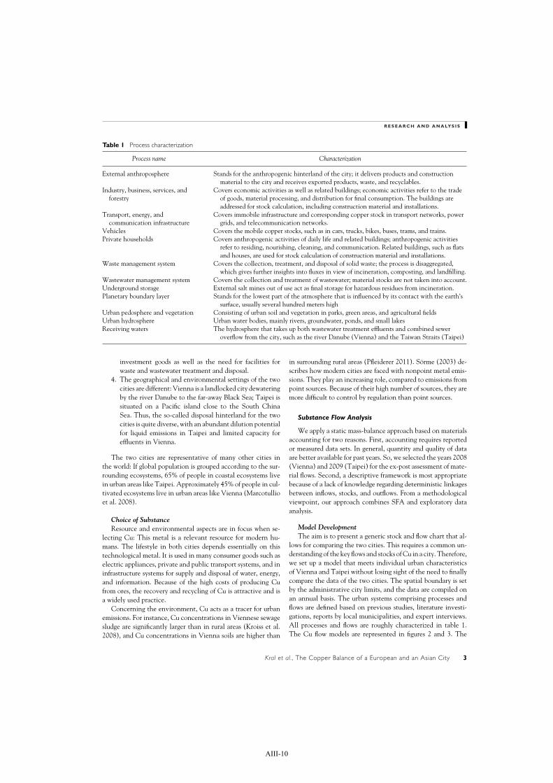
R E S E A R C H A N D A N A LYS I S
Table 1 Process characterization
Process name Characterization
External anthroposphere Stands for the anthropogenic hinterland of the city; it delivers products and constructionmaterial to the city and receives exported products, waste, and recyclables.
Industry, business, services, andforestry
Covers economic activities as well as related buildings; economic activities refer to the tradeof goods, material processing, and distribution for final consumption. The buildings areaddressed for stock calculation, including construction material and installations.
Transport, energy, andcommunication infrastructure
Covers immobile infrastructure and corresponding copper stock in transport networks, powergrids, and telecommunication networks.
Vehicles Covers the mobile copper stocks, such as in cars, trucks, bikes, buses, trams, and trains.Private households Covers anthropogenic activities of daily life and related buildings; anthropogenic activities
refer to residing, nourishing, cleaning, and communication. Related buildings, such as flatsand houses, are used for stock calculation of construction material and installations.
Waste management system Covers the collection, treatment, and disposal of solid waste; the process is disaggregated,which gives further insights into fluxes in view of incineration, composting, and landfilling.
Wastewater management system Covers the collection and treatment of wastewater; material stocks are not taken into account.Underground storage External salt mines out of use act as final storage for hazardous residues from incineration.Planetary boundary layer Stands for the lowest part of the atmosphere that is influenced by its contact with the earth’s
surface, usually several hundred meters highUrban pedosphere and vegetation Consisting of urban soil and vegetation in parks, green areas, and agricultural fieldsUrban hydrosphere Urban water bodies, mainly rivers, groundwater, ponds, and small lakesReceiving waters The hydrosphere that takes up both wastewater treatment effluents and combined sewer
overflow from the city, such as the river Danube (Vienna) and the Taiwan Straits (Taipei)
investment goods as well as the need for facilities forwaste and wastewater treatment and disposal.
4. The geographical and environmental settings of the twocities are different: Vienna is a landlocked city dewateringby the river Danube to the far-away Black Sea; Taipei issituated on a Pacific island close to the South ChinaSea. Thus, the so-called disposal hinterland for the twocities is quite diverse, with an abundant dilution potentialfor liquid emissions in Taipei and limited capacity foreffluents in Vienna.
The two cities are representative of many other cities inthe world: If global population is grouped according to the sur-rounding ecosystems, 65% of people in coastal ecosystems livein urban areas like Taipei. Approximately 45% of people in cul-tivated ecosystems live in urban areas like Vienna (Marcotullioet al. 2008).
Choice of SubstanceResource and environmental aspects are in focus when se-
lecting Cu: This metal is a relevant resource for modern hu-mans. The lifestyle in both cities depends essentially on thistechnological metal. It is used in many consumer goods such aselectric appliances, private and public transport systems, and ininfrastructure systems for supply and disposal of water, energy,and information. Because of the high costs of producing Cufrom ores, the recovery and recycling of Cu is attractive and isa widely used practice.
Concerning the environment, Cu acts as a tracer for urbanemissions. For instance, Cu concentrations in Viennese sewagesludge are significantly larger than in rural areas (Kroiss et al.2008), and Cu concentrations in Vienna soils are higher than
in surrounding rural areas (Pfleiderer 2011). Sorme (2003) de-scribes how modern cities are faced with nonpoint metal emis-sions. They play an increasing role, compared to emissions frompoint sources. Because of their high number of sources, they aremore difficult to control by regulation than point sources.
Substance Flow Analysis
We apply a static mass-balance approach based on materialsaccounting for two reasons. First, accounting requires reportedor measured data sets. In general, quantity and quality of dataare better available for past years. So, we selected the years 2008(Vienna) and 2009 (Taipei) for the ex-post assessment of mate-rial flows. Second, a descriptive framework is most appropriatebecause of a lack of knowledge regarding deterministic linkagesbetween inflows, stocks, and outflows. From a methodologicalviewpoint, our approach combines SFA and exploratory dataanalysis.
Model DevelopmentThe aim is to present a generic stock and flow chart that al-
lows for comparing the two cities. This requires a common un-derstanding of the key flows and stocks of Cu in a city. Therefore,we set up a model that meets individual urban characteristicsof Vienna and Taipei without losing sight of the need to finallycompare the data of the two cities. The spatial boundary is setby the administrative city limits, and the data are compiled onan annual basis. The urban systems comprising processes andflows are defined based on previous studies, literature investi-gations, reports by local municipalities, and expert interviews.All processes and flows are roughly characterized in table 1.The Cu flow models are represented in figures 2 and 3. The
Kral et al., The Copper Balance of a European and an Asian City 3
AIII-10

R E S E A R C H A N D A N A LYS I S
Figure 2 System “copper flows and stocks in Vienna” for the year 2008. Values for flows and changes in stocks are given in grams percapita per year (g/cap/yr) and for stocks in grams per capita (g/cap). The flows are represented as Sankey arrows proportional to the flowrate; figures for stocks are given within the “process” boxes. Numbers have been rounded.
Figure 3 System “copper flows and stocks in Taipei” for the year 2009. Values for flows and changes in stocks are given in grams percapita per year (g/cap/yr) and for stocks in grams per capita (g/cap). The flows are represented as Sankey arrows proportional to the flowrate; figures for stocks are given within the “process” boxes. Numbers have been rounded.
4 Journal of Industrial Ecology
AIII-11
R E S E A R C H A N D A N A LYS I S
Supporting Information on the Web (see section 2.2.2.1) pro-vides additional, comprehensive descriptions for all flows andstocks.
Model Equations and Data AcquisitionThe following model equations are used to calculate each
flow and stock:
mflow = f (p1, p2, p3, . . . , pi )
mstock = f (q1, q2, q3, . . . , qi )
where m f l ow is the Cu flux rate [mass/time], mstock is the Custock [mass], pi is the input parameter for m f l ow, and qi is theinput parameter for mstock . The input parameters pi and qi
are assumed to be normally distributed with N(m pi , s pi ) andN(mqi , sqi ). The mean values m and the standard deviation sare determined as follows:
� m is determined by data mining according to Mansson(2009). The data acquisition procedure prioritizes abottom-up approach for both cities. Data availability,quantity, and quality vary between each city. They areeven manifold within each city depending on the typeof flow and stock. As a common denominator, input pa-rameters representing city characteristics are documentedin official statistics. Import data are established throughdownscaling national import and export statistics. Theallocation to city internal processes is based on the globalsector share of Cu products and estimations based on localwaste statistics. Cu content in products is compiled fromliterature data, local consumption, and waste statistics.Waste flows are documented in statistics provided by pub-lic and private waste companies. Cu fluxes entering andleaving waste management plants, such as incineratorsand waste water treatment plants, are documented in sci-entific reports conducted by the city authority. Emissionflows are estimated by the compilation of literature dataand inventory databases, such as Ecoinvent. Cu stocksin technical infrastructures are estimated with networklengths and corresponding specific masses. In Vienna,stocks in buildings are based on Swiss per capita dataand those in Taipei are based on proxy data from otherTaiwanese cities.
� s is derived from the uncertainty factor u f accord-ing to data vagueness concept from Hedbrant andSorme (2001): s p = m p ∗ u f −1
2 sq = mq ∗ u f −12 with
u f = 1 + 0.0036 ∗ e1.105∗l . The uncertainty level l rangesfrom “1” to “5” and depends on the classification of thedata source. For example, official statistics on local levelare assumed to have low uncertainties (l = 1). Anotherexample is official statistics on the national level down-scaled to the local level with a higher level of uncertainty(l = 3).
The mean value and standard deviation of each flow(mm f l ow
, sm f l ow) and stock (mmstock , smstock ) is computed with
Monte Carlo simulation by taking into account the model equa-tions and the distribution functions of the input parameterspi
and qi .The documentation of the SFA model is given in the Sup-
porting Information on the Web. It includes section 2.2.2.1with a comprehensive description of flows and stocks for bothcities. Sections 2.2.2.2 and 2.2.2.3 address the city of Vienna,including two tables: one for the model equations and one forthe input parameters. Section 2.2.2.4 provides the backgrounddata for the city of Taipei.
Balance EquationsWe use static model architecture and apply the mass balance
principle on each process:
0 = minput − moutput + mstock
where mi nput is the annual input flow, moutput is the annualoutput flow, and ms tock is the alteration of stock. Because mul-tiple data sources are used, data quality and quantity are het-erogeneous. Consequently, contradictions in fulfilling the massbalance criteria occur. To overcome this gap, we applied thefreeware, STAN (Cencic 2012). It uses data reconciliation withan algorithm based on the error propagation law.
Stock and Flow Charts of Vienna and TaipeiFigures 2 and 3 show the annual Cu SFA charts. A full
list of unbalanced flows and balanced results is provided in theSupporting Information on the Web (see section 2.3).
Data Analysis and Indicator Selection
Exploratory data analysis stands for analyzing data sets tosummarize their main characteristics in an easy-to-understandform. We use this tool in combination with indicators for com-parative assessment of individual Cu flow data. An indicator isdefined to be one or several “observed variables that are usedto report a non observable reality” (Loiseau et al. 2012, 214).Our set of indicators represents the interaction of substanceswithin and between the anthroposphere and the environmentand form, in part, a base for policy support and decision makingfor substance management, recycling, and waste management.Table 2 compiles eight indicator groups, including 13 indica-tors in total. Seven relate to resource efficiency (RE), six relateto environmental protection (EP). The calculation routine isbased on the final Cu balances in each city, which comprise 42flows and four stocks each (figures 2 and 3).
Results and Discussion
Overview
Table 2 presents the computed indicator results, includingmean value and standard deviations as well as normalized in-dices on a per capita basis.
Kral et al., The Copper Balance of a European and an Asian City 5
AIII-12

R E S E A R C H A N D A N A LYS I STa
ble
2In
dica
tors
and
thei
rva
lues
for
Vie
nna
and
Taip
ei
Abs
olut
eva
lues
Nor
mal
ized
valu
eson
ape
rca
pita
base
Vie
nna
Tai
pei
Vie
nna
Tai
pei
No.
Indi
cato
rSc
ope
Uni
tM
ean
Dev
(%)
Mea
nD
ev(%
)U
nit
Mea
nD
evM
ean
Dev
IIm
port
sint
oth
eci
ties
RE
t/yr
20,6
448
28,8
4712
kg/c
ap/y
r12
.30.
911
.11.
4
IISt
ocks
and
chan
gesi
nst
ocks
––
––
––
––
––
–
Pres
entu
rban
stoc
kR
Et
298,
000
1372
,051
21kg
/cap
178
2428
6
Abs
olut
ech
ange
inst
ock
RE
t/yr
5,53
543
18,4
5327
kg/c
ap/y
r3.
31.
47.
11.
9
Rel
ativ
ech
ange
inst
ock
RE
%2
n.q.
26n.
q.–
––
––
III
Was
tesa
ndem
issi
ons
t/yr
12,3
705
2,45
06
kg/c
ap/y
r7.
40.
40.
90.
1
Solid
was
teR
Et/
yr12
,337
52,
437
6kg
/cap
/yr
7.4
0.4
0.9
0.1
Uni
nten
tion
alem
issi
ons
EPt/
yr28
1013
6kg
/cap
/yr
0.01
62
×10
−30.
005
3×
10−4
Inte
ntio
nale
mis
sion
sEP
t/yr
59
00
kg/c
ap/y
r0.
003
3×
10−4
00
IVR
atio
nonp
oint
emis
sion
sto
tota
lem
issi
ons
EP%
51n.
q.12
n.q.
––
––
–
VFl
owst
osi
nks
t/yr
14,9
356
10,4
0213
kg/c
ap/y
r8.
90.
54.
00.
5
Ant
hrop
ogen
icR
Et/
yr14
,924
610
,390
13kg
/cap
/yr
8.9
0.5
4.0
0.5
Envi
ronm
enta
lEP
t/yr
128
413
kg/c
ap/y
r7.
0×
10−3
0.6
×10
−31
×10
−30.
2×
10−3
VI
Acc
umul
atio
nin
urba
nso
ilEP
%0.
07n.
q.0.
03n.
q.–
––
––
VII
Rem
oval
effic
ienc
yby
was
tew
ater
man
agem
ent
EP%
65%
n.q.
74%
n.q.
––
––
–
VII
IC
oppe
rcon
tent
inbo
ttom
ash
RE
t/yr
1,09
77
165
34kg
/cap
/yr
0.65
50.
043
0.06
30.
021
Not
es:
RE
=re
sour
ceef
ficie
ncy;
EP=
envi
ronm
enta
lpr
otec
tion
;mea
n=
mea
nva
lue;
dev
=st
anda
rdde
viat
ion;
n.q.
=no
tqu
anti
fied;
—=
not
rele
vant
;t=
met
ric
tons
;t/y
r=
met
ric
tons
per
year
;%
=pe
rcen
t;kg
/cap
/yr=
kilo
gram
sper
capi
tape
ryea
r.
6 Journal of Industrial Ecology
AIII-13

R E S E A R C H A N D A N A LYS I S
0
10
20
30
40
50
60
70
80
90
100
Buildings Infrastructure Vehicles Consumergoods
kg C
u/c
ap
Vienna Taipei
Figure 4 Comparison of copper stocks in Vienna (total stock:178 kilograms per capita [kg/cap]) and Taipei (total stock:28 kg/cap). Whereas the residence time of copper in buildings andinfrastructure is long (10 to 100 years), it is shorter in vehicles andconsumer goods (less than 10 years).
Comparative Assessment and Interpretation of CopperBalances
In the following sections, indicators and their relevance areexplained in detail, and results as well as conclusions are pre-sented.
Imports into the Cities (I)Net imports represent the demand and consumption patterns
and relate to resource supply as well as to the city’s economicsituation. In both consumption-oriented cities with a compar-atively high gross domestic product (GDP), Cu is mainly usedin infrastructure and consumer goods. Similar amounts of Cuare imported for Vienna (12 ± 1 kilograms per capita per year[kg/cap/yr]) and Taipei (11 ± 1 kg/cap/yr); both cities rely heav-ily on Cu import from outside regions. The observed net importrates are six times higher than the average global per capitaconsumption (Graedel et al. 2004; United Nations 2010).
Stocks and Changes in Stocks (II)Three indicators focus on stocks: (1) the present urban stock
and (2) the absolute and (3) relative change in stock.A large part of Cu imports turns into stocks. There are Cu
stocks of 178 ± 23 kg/cap in Vienna and of 28 ± 6 kg/capin Taipei. Similar stocks have been found for other cities inEurope (Sorme et al. 2001a) and in Asia (Zhang et al. 2012).The two cities show different shares of individual Cu stocks(figure 4). Vienna hosts 80% of Cu in long-term assets. Heatingsystems as well as networks for electricity and telecommuni-cation are the main Cu carriers. In contrast, Taipei (1) has amuch shorter history in urban development and (2) buildingslack heating systems. Forty-eight percent of the Cu is storedin long-term goods, such as infrastructures and buildings, and52% are related to consumer goods, such as air conditioners,cars, and scooters. As a summary, the two cities show marked
differences in quantity and relative share in individual sector:Vienna is rich in Cu, and urban mining hotspots are identifiedin long-term assets, such as infrastructure and building com-ponents. In Taipei, consumer goods have more importance forrecovering secondary Cu.
Stock changes denote the annual accumulation or deple-tion of Cu in various stocks, such as buildings, infrastructure,vehicles, and consumer goods. The indicator represents theeconomic and technological pattern of a city: As long as a citygrows, the input will always be bigger than the output, resultingin a stock increase. An exception is given for a material that issubstituted by another, or that is phased out, such as cadmium.For such substances, the input can be smaller than the output,resulting in stock depletion.
The total annual growth rate of the Cu stock is 7 ± 2 kg/capin Taipei and 3 ± 1 kg/cap in Vienna. In both cities, con-sumer stocks increase. In Taipei, more Cu is accumulated inprivate households than infrastructure and vehicles, with salesin the household electronic sector and in electronic appliancesin vehicles as the main drivers.
The relative change in stock puts the absolute change instock (in kg/cap/yr) in relation to present stock (in kg/cap).The relative accumulation of Cu in the stock of Taipei (26%)is more than 10 times higher than in Vienna (2%). In otherwords, the Cu stock in Vienna is already on a high level andgrows only moderately. In Taipei, there is a backlog of demandin the city, resulting in a much faster stock increase, whichis mainly a result of private households. For Taipei, the Cuconsumption in private households is five times higher thanin Vienna, where Cu turnover is determined by maintainingrelatively large stocks.
Wastes and Emissions (III)This category comprises three indicators: (1) the amount of
Cu in solid wastes, including scrap for recycling, and (2) inten-tional and (3) unintentional emissions. “Intentional emissions”denominate Cu flows resulting from applications that transport,on purpose, Cu into the environment, such as Cu use in agricul-ture as a fungicide. “Unintentional emissions” are by-productsresulting from other processes, such as wastewater from house-holds and industry, the release of Cu from catenary wires, orbrake pads during the operation of vehicles. These emissionspose a potential threat to the environment.
In Vienna, the total flow of Cu resulting from wastes andemissions is eight times higher than in Taipei (7.4 ± 0.4 vs.0.9 ± 0.1 kg/cap/yr). In both cities, solid-waste–borne Cu dom-inates emissions by more than 99%. Unintentional emissionsfollow next with less than 1%. These findings are in line withresults from a study on dissipative emissions in the United States(Lifset et al. 2012). Lifset and colleagues point out that the re-cycling rate would increase only by 0.5% if dissipative losseswould be recovered and included in recycling, too.
The household waste fractions of Vienna and Taipei are sim-ilar (1.0 ± 0.06 vs. 0.7 ± 0.02 kg/cap/yr). In contrast, the frac-tions from the industrial and construction sector and waste ve-hicles differ significantly between Vienna (6.4 ± 0.4 kg/cap/yr)
Kral et al., The Copper Balance of a European and an Asian City 7
AIII-14

R E S E A R C H A N D A N A LYS I S
0
2
4
6
8
10
12
14
Vienna Taipei Vienna TaipeiWaste water system Urban soil
g C
u /c
ap/y
r
non-point sources
point sources
Figure 5 Comparison of copper flows into sinks in Vienna(14 grams per capita per year [g/cap/yr]) and Taipei (5 g/cap/yr)divided into flows entering the wastewater system and soil.Nonpoint sources address waterborne copper in surface runoff andinclude roof runoff, brake and tire wear from cars, catenary wear,and atmospheric deposition. Point sources relate to waterborneemissions from industry and household, such as urine, feces,consumer products, and pipe corrosion.
and Taipei (0.2 ± 0.1 kg/cap/yr). These findings may be theresult of the following three reasons. First, the large and com-paratively old stock of Cu in infrastructure and buildings ofVienna must be continuously replaced and acts a source of Cuwaste. Second, Taipei has installed a zero waste policy attempt-ing to reduce Cu waste from production. As a third source ofuncertainty, statistical data from the two cities about wasteflows from the industrial sector have been collected by differingmethodologies.
Unintentional Cu emissions in Vienna are three times largerthan in Taipei (16 ± 2 grams per capita per year [g/cap/yr] vs.5 ± 0.3 g/cap/yr). Both airborne emissions and surface runoff inVienna are approximately 12 times higher than in Taipei. Thisis because of a higher amount of car mileage and correspondingbreak wear, catenary wear which is inexistent in Taipei, andthe utilization of Cu as a roof and gutter material in Vienna.
Ratio of Nonpoint Emissions to Total Emissions (IV)Bergback (1992) and Sorme and colleagues (2001b) refer to
the increasing relevance of nonpoint emissions from the usephase of goods when compared to industrial point source emis-sions. They report a significant amount of nonpoint emissionsfor Stockholm and Sweden. The investigators state the difficul-ties when attempting to regulate nonpoint emissions, such asabrasion from brake pads or corrosion from roofs and gutters.Therefore, we choose as an indicator the proportion of non-point emissions to total emissions. Results show that the ratioof nonpoint emissions to total emissions differs between 51%in Vienna and 12% in Taipei (figure 5).
In both cities, the wastewater system receives (1) most of theCu emissions in town (Vienna, 87%; Taipei, 97%) and (2) moreCu from point sources than from nonpoint sources (Vienna,
57%; Taipei, 91%). Point sources include Cu inputs into thewastewater from private and commercial facilities. In Vienna,approximately 20% of point emissions originate from feces,urine, consumer products, and kitchen waste, 20% from corrod-ing water pipes, and the remaining 60% are related to industrialactivities. In Taipei, the relevance of individual point sourcesis not fully determined because of a lack of local information.
Nonpoint sources cover brake and tire wear, catenary wear,and roof runoff. In Vienna, the annual Cu flow from nonpointsources is 13 times larger than in Taipei (7.3 vs. 0.6 g/cap/yr).The higher rate is the result of the presence of an extensivetram network, the popularity of Cu roofs and gutters, andhigher emissions from low-duty vehicles. On a per capita basis,the Viennese Cu flow into soil is approximately 15 larger thanthat in Taipei (1.65 vs. 0.11 g/cap/yr).
Two conclusions can be drawn: First, nonpoint emissionpatterns play an important role in the case of Vienna,confirming the result of the Swedish studies (Sorme et al.2001b; Hjortenkrans et al. 2007). This requires that cityauthorities develop specific long-term strategies for protectingthe environment from nonpoint emissions. Second, becauseof high ratios of sealed and drained area, the majority of Cuflows is waterborne and collected by the sewer system. Effectiveend-of-pipe technologies, such as appropriate sewage treatmentplants, are needed for separating heavy metals in order tocontrol the impact on receiving waters.
Flows to Sinks (V)For this study, anthropogenic sinks and environmental sinks
have been taken into account as indicators. In both cities, themain Cu flows to sinks stay within the anthroposphere (morethan 99.9%), and less than 0.1% of the total processed out-put accumulates in the environment (Vienna, 0.08%; Taipei,0.03%). Figure 6 summarizes the flows to the main sinks.
From the city point of view, anthropogenic sinks consist of(1) landfills within the city limits and of (2) goods, wastes, andrecyclables that are processed outside of Vienna and Taipei,respectively. Landfills containing Cu in municipal solid waste(MSW) and bottom ash from MSW incineration (see discus-sion below on “Copper content in bottom ash”) belong to theinternal anthroposphere. Cu from recyclables is recovered inthe external anthroposphere because there are no Cu recyclingfacilities within the two investigated cities. The largest amountof Cu leaves the city as a product or solid waste. Taipei exports78% of Cu in a product form and Vienna 81% of Cu as waste,including recyclables.
Environmental sinks consist of receiving waters and theurban soil within the city limits. The efficiency of the totalwastewater system, in terms of separating and directing Cu toappropriate sinks and its relevance for city planning, is fur-ther examined when the indicator “Technical efficiency of thewastewater system” is discussed below. The soil accumulatingCu by deliberate, as well as unintentional, emissions is includedin the following discussion of the indicator “Accumulation inurban soil.” The atmosphere as a sink has been neglected as aresult of the short residence time of Cu in the air.
8 Journal of Industrial Ecology
AIII-15

R E S E A R C H A N D A N A LYS I S
0
1
2
3
4
5
6
7
8
9
10
0
1
2
3
4
5
6
7
8
9
10
Vienna Taipei Vienna Taipei Vienna Taipei Vienna Taipei
External anthroposphere Landfill Receiving water Urban soil
sknis latnemnorivnEsknis cinegoporhtnA
Envi
ronm
enta
l sin
ksg
Cu/
cap/
yr
Ant
hrop
ogen
ic s
inks
kg C
u/ca
p/yr
Exported products
Exported waste including recyclables
Bottom-ash and residues from air-pollution-control
Filter cake
Combined sewer overflow
Effluents
Surface runoff (seperated sewer system)
Compost
Atmospheric deposition on urban soil
Figure 6 Comparison of copper flows to anthropogenic and environmental sinks in Vienna. The bars for the “anthropogenic sinks” aregiven in kilograms per capita per year (kg/cap/yr) and those for the “environmental sinks” in grams per capita per year (g/cap/yr). The“External anthroposphere” consists of the hinterland and includes exterior consumption, recycling processes, and underground storage sitesoutside of Vienna and Taipei. “Receiving water” stands for the river Danube and the Danshui River, respectively.
Accumulation in Urban Soil (VI)The disparity between the levels of Cu in urban and ru-
ral areas has been known for many decades. See, for instancePurves (1966, p. 1077) who is referring to “evidence of slowpoisoning of the soil environment in built-up areas.” The needfor observing urban soil conditions for sustainable, long-termland management is well established (e.g., Wong et al. 2006;Johnson et al. 2011), mostly because analysis of soil samplesoccasionally showed elevated concentrations compared to ruralareas (Pfleiderer 2011; Jien et al. 2011). Because of the lack ofsuch systematic monitoring in Vienna and Taipei, we used asimplified indicator by relating the annual Cu load to the ex-isting Cu stock in the top 30 centimeters of soil of greenspaceareas within the city boundaries. Results indicate slow Cu ac-cumulation for the two city soils. The higher accumulation ratein Vienna (0.07% per year) versus Taipei (0.03% per year)may well resemble the bigger emission rate into the air by theAustrian city. Both countries and cities fall short of legal thresh-old values regarding substance concentrations in urban soil.
Based on the SFA data and the fact that both cities aresituated in service-based and not industrial regions, it can beconcluded that the accumulation of Cu in the soil of the twocities is small. Little effects on the pedosphere are expected inthe next few centuries. Nevertheless, because there are no ap-propriate surveying programs in place, it may be that hotspotsin the soil exist either by local emissions, geological anomalies,
or former anthropogenic inputs. Because the Cu metabolismof Vienna is distinctly different, with more Cu on the sur-face of buildings and more incorporated in traffic systems, aneffective monitoring program should be established first in Vi-enna in order to ensure that reference values are not surpassed.Site-specific reference values, based on geogenic backgroundconcentrations, are actually being developed in a project called“urban geochemistry of Vienna” (Pfleiderer 2011).
Removal Efficiency by Wastewater Management (VII)In Germany, approximately 35% of Cu input into rivers
originates from urban areas (Blondzik et al. 2004). The type ofsewer system, its leakage rates, and the treatment technologydetermine the heavy metal discharge into the hydrosphere. Toestimate the efficiency of the wastewater system regarding Curemoval, we relate Cu removed by the wastewater treatment(wwt) system and contained in sewage sludge to the totalamount of Cu that has been introduced into the sewer system.SFA calculations yield Cu removal efficiencies of 74% forTaipei and 65% for Vienna. The remaining 26% and, respec-tively, 35% enter receiving waters by combined sewer overflow,wwt effluent, and surface runoff. Both surface runoff collectedby separate sewer systems and combined sewer overflow reachreceiving waters directly without treatment. The lower removalefficiency in Vienna is likely the result of larger nonpointemissions and additional Cu loads from the combined sewer
Kral et al., The Copper Balance of a European and an Asian City 9
AIII-16

R E S E A R C H A N D A N A LYS I S
overflow. Based on these results, the following conclusions canbe drawn:
� Wwt systems design: In order to decrease Cu loadings intothe hydrosphere, reduction as well as collection of non-point Cu emissions and high removal rates by wwt is im-portant. The comprehensive design of the entire wastew-ater collection and treatment system becomes crucial forservice-oriented cities where nonpoint sources are thedominant cause of emissions.
� Monitoring: There is a lack of accurate data with knownuncertainties regarding surface runoff, combined seweroverflow, and stormwater overflow. Few cities establishcomplete water balances, including collected and un-collected as well as treated and untreated waters andwastewaters. We recommend establishing water balancesfor cities and using them as a base for decisions regardingenvironmental management. The city of Berlin serves asan example for a sophisticated precipitation runoff modelbased on land use and resulting in estimations of location-based surface runoff (City of Berlin 2012b, 2012a).
� Environmental risk assessment: Cities in general dependon dilution potentials in their hinterland. Vienna usesthe river Danube and Taipei the Danshui River for dissi-pation of Cu contained in purified sewage. Despite thatone third to one fourth of sewage-borne Cu is releasedto the receiving waters, existing environmental qualitystandards are observed in both cases. For sediments of theriver and sea, there is a lack of both legal standards as wellas consistent monitoring data about Cu concentrations(e.g., for Vienna, Kavka et al. 2000). In order to preventfuture overloading, environmental fate and impact mod-els could be used for predicting the evolution of heavymetal concentrations over time.
Copper Content in Bottom Ash (VIII)In both cities, municipal solid waste is incinerated in waste to
energy plants. During incineration, most of the Cu contained inMSW is transferred to bottom ash. To recover Cu from bottomash offers two advantages: First, it contributes to resource con-servation. Second, it is instrumental for minimizing Cu flows tothe environment in case bottom ash is landfilled or reused as aconstruction material.
In Vienna, bottom ash is stabilized with cement and dis-posed of in the municipal landfill. In Taipei, bottom ash isused as a base material for road construction as well as a fineaggregate in asphalt (Taipei County Government 2010). Theper capita Cu flux in Vienna is approximately 10 times largerthan in Taipei (655 ± 43 vs. 63 ± 21 g/cap/yr), correspond-ing to approximately 5% (Vienna) and 1% (Taipei) of annualCu consumption. The market value of Cu contained in bot-tom ash equals roughly US$8.8 million per year in Vienna andUS$1.4 million per year in Taipei.
As a result of the value of Cu and other metals, economicincentives exist to recover valuable elements, such as Cu, alu-minum, gold, and silver, from bottom ash. Substance concen-
trations are several times higher than in natural ores (Simon1996; Jordi 2004) and can be considerably increased by bottomash treatment (e.g., Muchova et al. 2009; Morf et al. 2013; Shenand Forssberg 2003). Recent experiences favor dry discharge ofbottom ash for efficient recovery of nonferrous metals (Morfet al. 2013). This technology is not yet implemented in Viennaand Taipei.
Another means to recover valuable metals from MSW islandfill mining, that is, the excavation of materials from oldMSW or bottom ash landfills. From an economic point of view,landfill mining appears to be attractive only if additional val-ues are created. This could be driven by gaining new land forbuilding sites or reduced costs for long-term landfill after care.Thus, recovery projects that aim exclusively at recovering re-sources are rare (Holzle 2010). Assuming a period of 20 yearsand a waste generation rate of one kilogram of MSW per per-son and day, 24,000 tonnes1 of Cu with an economic value ofUS$200 million have been accumulated in Viennese landfills.
In addition to recovery of Cu from bottom ash and landfills,Cu can also be recovered by separate collection of Cu con-taining waste fractions, such as waste electrical and electronicequipment. In fact, this practice is widely applied and is themost favored by European waste policy. For best effectivenessof a comprehensive Cu recovery system, the main carriers ofCu (Morf and Taverna 2006), as well as the efficiencies andcosts of recovery technologies, must be known. It remains to bedetermined which of the recovery pathways reaches the goalsof waste management “resource recovery” and “environmentalprotection” at the least costs.
Conclusions
This article presents the results of investigations into ur-ban Cu flows and stocks in two different cities. It provides astarting point for comparing additional cities and metals. Themass balance approach, focusing on the main processes, Cuflows, and stocks, goes beyond the city as a black-box model.To our knowledge, this study is the most comprehensive Cubalance on the urban level, encompassing Cu flows from im-ports to stocks in use and exports. Also, it is the first com-parison of the Cu metabolism of two cities. Based on the re-sults, we discuss reasons for differences in the Cu balances ofVienna and Taipei and give recommendations for the man-agement of Cu as a resource and potential environmentalpollutant.
First, we find typical characteristics in the dynamics of Custock changes. Rapid growth in a young city such as Taipeiis characterized by low amounts of Cu stocks and relativelyhigh annual stock increases. In contrast, Cu stocks in olderVienna are relatively high, and thus the relative stock changeis smaller than in Taipei. Cu demand and disposal in Vienna ismainly the result of maintenance and replacement. The relativeimportance of Cu in consumer goods decreases.
Second, much Cu is recycled, but there are still recoverypotentials available. Bottom ash from waste incineration is an
10 Journal of Industrial Ecology
AIII-17

R E S E A R C H A N D A N A LYS I S
example for both cities. In order to reach sustainability goalssuch as resource conservation and long-term environmentalprotection, recovering more Cu from MSW and other wastesis mandatory. On the one hand, especially if combined withthe recovery of additional metals such as aluminum, gold, andsilver, this may result in economic benefits. On the other hand,separation of Cu together with other metals, such as chromium,lead, and cadmium reduces the concentrations of heavy metalsin bottom ash, making this material more suitable for utilizationas a construction material.
Third, some Cu is emitted diffusively by wear, corrosion, andweathering of Cu built into infrastructure, transport systems,and others. These emissions partly enter the wastewater systemand partly accumulate in the urban soil. Nonpoint emissionsare not yet in the focus of urban governance, even though, forexample, the European Union urges member states to take non-point emission into account. Based on the experiences of thestudies in Stockholm, Vienna, and Taipei, it is recommendedto monitor the concentrations of Cu and other heavy metals inurban soils and sediments by a combination of SFA and directmeasurements.
Fourth, designing urban wastewater systems in a compre-hensive way is crucial for minimizing the loading of receivingwaters with Cu and other heavy metals. The combination ofwastewater collection systems and treatment technologies de-termine the total efficiency in terms of removing pollutants. Foreffective control of heavy metal flows to receiving waters, theentire systems performance is more important than the removalefficiency of wastewater treatment alone.
Fifth, this study has shown that transnational collabo-ration yields new insights into the substance balances ofcities. Authorities and researchers profit from each otherthrough a common research framework for comparing urbanmetabolism data. We recommend sharing experiences and dis-cussing methodology for urban metabolism studies and de-veloping common generic models as well as data acquisitionprocedures.
Acknowledgments
This study was supported by the Austrian Science Fund(FWF; I 549-N21) and the Taiwanese National Research Coun-cil (NSC; NSC99-2923-E-002-006-MY3).
Note
1. The term tonne refers to metric ton. One tonne (t) = 103 kilograms(kg, SI) ≈ 1.1 short tons.
References
Agudelo-Vera, C. M., A. R. Mels, K. J. Keesman, and H. H. M. Ri-jnaarts. 2011. Resource management as a key factor for sustain-able urban planning. Journal of Environmental Management 92(10):2295–2303.
Baccini, P. and H. P. Bader. 1996. Regionaler Stoffhaushalt. [Regionalmetabolism.] Heidelberg, Berlin, Oxford: Spektrum, Akad, Ver-lag.
Baccini, P. and P. H. Brunner. 2012. Metabolism of the anthroposphere:Analysis, evaluation, design, 2nd ed. Cambridge, MA, USA: MITPress.
Bergback, B. 1992. Industrial metabolism: The emerging landscapeof heavy metal emissions in Sweden. Ph.D. thesis, LinkopingUniversity, Linkoping, Sweden.
Bergback, B., K. Johansson, and U. Mohlander. 2001. Urban metalflows—A case study of Stockholm. Review and conclusions. Wa-ter, Air, and Soil Pollution: Focus 1(3): 3–24.
Blondzik, K., U. Claussen, C. Full, and J. Heidemeier. 2004. Umwelt-politik: Die Wasserrahmenrichtlinie—Neues Fundament fur denGewasserschutz in Europa. [Environmental policy: The waterframework directive—A new baseline for water protection in Eu-rope.] Berlin: Bundesministerium fur Umwelt, Naturschutz undReaktorsicherheit.
Brunner, P. H. and H. Rechberger. 2004. Practical handbook of materialflow analysis. Boca Raton, FL, USA: CRC Press.
CEPD (Council for Economic Planning and Development). 2012. Es-timation of population in Taiwan from 2012 to 2060 (in Chinese).Taipei: CEPD, Council for Economic Planning and Develop-ment, Executive Yuan.
Cencic, O. 2012. Software platform STAN (short for subSTance flowANalysis). www.stan2web.net. Accessed 28 September 2012.
Chen, W.-Q. and T. E. Graedel. 2012. Anthropogenic cycles of theelements: A critical review. Environmental Science & Technology46(16): 8574–8586.
City of Berlin. 2012a. Flow chart of the ABIMO model. www.stadtentwicklung.berlin.de/umwelt/umweltatlas/extra/213eb02.htm. Accessed 11 January 2013.
City of Berlin. 2012b. Berlin environmental atlas—Surface runoff,percolation, total runoff and evaporation from precipitation.www.stadtentwicklung.berlin.de/umwelt/umweltatlas/edb213_05.htm. Accessed 11 January 2013.
Geddes, P. 1885. An analysis of the principles of economics. Proceedingsof the Royal Society of Edinburgh Vol. XII, edited by Royal Societyof Edinburgh, Edinburgh, UK.
Graedel, T., D. Van Beers, M. Bertram, K. Fuse, R. Gordon, A.Gritsinin, A. Kapur, R. Klee, R. Lifset, and L. Memon. 2004.Multilevel cycle of anthropogenic copper. Environmental Science& Technology 38(4): 1242–1252.
Hedbrant, J. and L. Sorme. 2001. Data vagueness and uncertainties inurban heavy-metal data collection. Water, Air, & Soil Pollution:Focus 1(3): 43–53.
Henseler, G., R. Scheidegger, and P. H. Brunner. 1992. Die bestim-mung von Stoffflussen im Wasserhaushalt einer Region. [Deter-mination of material flux through the hydrosphere of a region.]Vom Wasser 78: 91–116.
Hertwich, E. and G. P. Peters. 2010. Multiregional Input-Output Database (OPEN:EU technical document). www.oneplaneteconomynetwork.org/resources/programme-documents/WP1_MRIO_Technical_Document.pdf. Accessed 2 December2012. Trondheim, Norway: One Planet Economy Network.
Hjortenkrans, D. S. T., B. G. Bergback, and A. V. Haggerud. 2007.Metal emissions from brake linings and tires: Case studies ofStockholm, Sweden 1995/1998 and 2005. Environmental Science& Technology 41(15): 5224–5230.
Kral et al., The Copper Balance of a European and an Asian City 11
AIII-18

R E S E A R C H A N D A N A LYS I S
Hoekstra, R. and J. C. J. M. van den Bergh. 2006. Constructing physicalinput-output tables for environmental modeling and accounting:Framework and illustrations. Ecological Economics 59(3): 375–393.
Holzle, I. 2010. Vom Deponieruckbau bis zum landfill mining—eine Synthese internationaler Untersuchungen. [Landfill disman-tling and landfill mining—A synthesis of international investiga-tions.] Osterreichische Wasser- und Abfallwirtschaft 62(7–8): 155–161.
Jien, S. H., C. C. Tsai, Z. Y. Hseu, and Z. S. Chen. 2011. Baselineconcentrations of toxic elements in metropolitan park soils ofTaiwan. Terrestrial and Aquatic Environmental Toxicology 5(1): 1–7.
Johnson, C. C., A. Demetriades, J. Locutura, and R. T. Ottesen (eds.).2011. Mapping the chemical environment of urban areas. Chichester,UK: John Wiley & Sons, Ltd.
Jordi, B. 2004. Recycling—die Rohstoffquelle der Zukunft.[Recycling—a future source of resources.] Magazin Umwelt1/2004: Produkte und Konsum. Bern, Schweiz: Bundesamt furUmwelt (BAFU).
Kavka, G., D. Kramer, P. Kreitner, R. Mauthner-Weber, G. Ofenboeck,and A. Rauchbuchl. 2000. Wasserbeschaffenheit und Gute derOsterreichischen Donau unter besonderer Berucksichtigung derlangzeitlichen Entwicklung. [Water quality of the Danube un-der long term considerations.] Wien: Bundesamt fur Wasser-wirtschaft.
Kroiss, H., L. S. Morf, C. Lampert, and M. Zessner. 2008. OptimiertesStoffflussmonitoring fur die Abwasserentsorgung Wiens. [Optimizedsubstance flow monitoring of the waste water treatment plant inVienna.] Vienna: Technische Universitat Wien.
Leontief, W. and D. Ford. 1972. Air pollution and the economic struc-ture: Empirical results of input-output computations. Fifth In-ternational Conference on Input-Output Techniques, January 1971,Geneva. Amsterdam: North Holland Publishing Company.
Lifset, R. J., M. J. Eckelman, E. M. Harper, Z. Hausfather, and G.Urbina. 2012. Metal lost and found: Dissipative uses and releasesof copper in the United States 1975–2000. Science of The TotalEnvironment 417–418: 138–147.
Lindqvist, A. and F. von Malmborg. 2004. What can we learn fromlocal substance flow analyses? The review of cadmium flows inSwedish municipalities. Journal of Cleaner Production 12(8–10):909–918.
Loiseau, E., G. Junqua, P. Roux, and V. Bellon-Maurel. 2012. Envi-ronmental assessment of a territory: An overview of existing toolsand methods. Journal of Environmental Management 112: 213–225.
Mansson, N. 2009. Substance flow analysis of metals and organic com-pounds in an urban area. Ph.D. thesis, School of Pure and AppliedNatural Sciences, University of Kalmar, Kalmar, Sweden.
Mansson, N., B. Bergback, D. Hjortenkrans, A. Jamtrot, and L. Sorme.2009. Utility of substance stock and flow studies. Journal of Indus-trial Ecology 13(5): 674–686.
Marcotullio, P. J., A. K. Braimoh, and T. Onishi. 2008. The impactof urbanization on soils. In Land use and soil resources, edited byA. K. Braimoh and P. L. G. Vlek. Dordrecht, the Netherlands:Springer Science+Business Media B.V.
Morf, L. S. and R. Taverna. 2006. Monitoringkonzept zur Ermit-tlung von Ursachen fur Veranderungen der Schwermetallgehalte imWiener Restmull. [Monitoring concept to investigate the change inheavy metal concentrations in residual waste of Vienna.] Zurich,Schweiz: GEO Partner AG Umweltmanagement.
Morf, L. S., R. Gloor, O. Haag, M. Haupt, S. Skutan, F. D. Lorenzo,and D. Boni. 2013. Precious metals and rare earth elements in
municipal solid waste—Sources and fate in a Swiss incinerationplant. Waste Management 33(3): 634–644.
Muchova, L., E. Bakker, and P. Rem. 2009. Precious metals in mu-nicipal solid waste incineration bottom ash. Water, Air, & SoilPollution: Focus 9(1–2): 107–116.
Nakamura, S. and Y. Kondo. 2009. Waste input-output analysis: Con-cepts and application to industrial ecology. In Eco-efficiency inindustry and science, Vol. 26, edited by A. Tukker. Dordrecht, theNetherlands: Springer Science+Business Media B.V.
Nakamura, S., K. Nakajima, Y. Kondo, and T. Nagasaka. 2007. Thewaste input-output approach to materials flow analysis. Journal ofIndustrial Ecology 11(4): 50–63.
Pfleiderer, S. 2011. Umweltgeochemie Stadtgebiet Wien. [Environ-mental geochemistry of the city of Vienna, restricted for publicaccess.] Seminar Ressourcenmanagement und Abfallwirtschaft [Sem-inar Resources and Waste Management], 4 June 2011, Vienna.
Purves, D. 1966. Contamination of urban garden soils with copper andboron. Nature 210(5040): 1077–1077.
Shen, H. and E. Forssberg. 2003. An overview of recovery of metalsfrom slags. Waste Management 23(10): 933–949.
Simon, F. G. 1996. Geld in der Kehrichtschlacke. [Money in bottom-ash.] Neue Zurcher Zeitung, Beilage Forschung und Technik, 134[Zurich], 6 December 1996.
Sorme, L. 2003. Urban heavy metals: Stocks and flows. Ph.D. thesis,The Tema Institute, Department of Water and EnvironmentalStudies, Linkoping University, Linkoping, Sweden.
Sorme, L., B. Bergback, and U. Lohm. 2001a. Century perspective ofheavy metal use in urban areas. A case study in Stockholm. Water,Air and Soil Pollution: Focus 1(3–4): 197–211.
Sorme, L., B. Bergback, and U. Lohm. 2001b. Goods in the anthro-posphere as a metal emission source: A case study of Stockholm,Sweden. Water, Air, and Soil Pollution: Focus 1(3): 213–227.
Statistik Austria. 2013. Vorausberechnete Bevolkerungsstruktur furWien 2011–2075 laut Hauptszenario. [Population outlook forVienna 2011–2075 according to the main scencario.] www.statistik.at/web_de/statistiken/bevoelkerung/demographische_prognosen/bevoelkerungsprognosen/index.html. Accessed 31January 2013.
Taipei County Government 2010. Decision analysis of bottom-ash Reusestrategic planning [in Chinese]. Taipei: Environmental ProtectionDepartment of Taipei County Government (New Taipei CityGovernment).
United Nations. 2010. World population prospects, the 2010 revision.http://esa.un.org. Accessed 16 January 2013.
Wong, C. S. C., X. Li, and I. Thornton. 2006. Urban environmentalgeochemistry of trace metals. Environmental Pollution 142(1): 1–16.
Zhang, L., Z. Yuan, and J. Bi. 2012. Estimation of copper in-usestocks in Nanjing, China. Journal of Industrial Ecology 16(2):191–202.
About the Authors
Ulrich Kral is a Ph.D. candidate at the Institute for WaterQuality, Resource and Waste Management, at Vienna Uni-versity of Technology, Vienna, Austria. Chih-Yi Lin is a re-search assistant in the Graduate Institute of EnvironmentalEngineering, National Taiwan University, Taipei, Taiwan. Atthe time of this study, Katharina Kellner was a research assistant
12 Journal of Industrial Ecology
AIII-19

R E S E A R C H A N D A N A LYS I S
at the Institute for Water Quality, Resource and Waste Man-agement, at Vienna University of Technology. She is currentlya business analyst at McKinsey & Company, Inc., Washing-ton, DC, USA. Hwong-wen Ma is a professor in the Graduate
Institute of Environmental Engineering, National Taiwan Uni-versity. Paul H. Brunner is a professor for waste managementand head of the Institute for Water Quality, Resource and WasteManagement, at Vienna University of Technology.
Supporting Information
Additional Supporting Information may be found in the online version of this article at the publisher’s web site:
Supporting Information S1: This supporting information provides a large quantity of background material that complementsthe methods and findings included in the main research article, including a compilation of 15 exemplary studies for copper(Cu) on an urban scale, comprehensive descriptions of all flows and stocks for the study, documentation on the substanceflow analysis (SFA) model used, and a full list of unbalanced flows and balanced results for this study.
Kral et al., The Copper Balance of a European and an Asian City 13
AIII-20

2013 Journal of Industrial Ecology – www.wileyonlinelibrary.com/journal/jie
Kral, U., C.-Y. Lin, K. Kellner, H.-W. Ma, P.H. Brunner. 2013. The copper balance of cities: Exploratory insights into a European and an Asian city. Journal of Industrial Ecology.
This supporting information provides a large quantity of background material that complements the methods and findings included in the main research article, including: a compilation of 15 exemplary studies for copper (Cu) on an urban scale; comprehensive descriptions of all flows and stocks for the study; documentation on the substance flow analysis (SFA) model used; and a full list of unbalanced flows and balanced results for this study.
AIII-21
2013 Journal of Industrial Ecology – www.wileyonlinelibrary.com/journal/jie
S 2
Table of Contents1. Introduction.................................................................................................................................................. 42. Material and methods .................................................................................................................................. 5
2.1 City selection and city characteristics ..................................................................................................... 52.2 Substance flow modeling ....................................................................................................................... 5
2.2.1 Model development ....................................................................................................................... 52.2.2 Model equations and data acquisition............................................................................................ 6
2.2.2.1 Flows & stock description for Vienna and Taipei ................................................................................6
2.2.2.1.1 Atmospheric Deposition (ADE PBLUHY, ADE PBLUPV, ADE PBLECO, ADE PBLPHH, ADE PBLTEC) .................... 62.2.2.1.2 Products (PRO EXAECO, PRO ECOPHH) ........................................................................................................... 62.2.2.1.3 Construction material (CON EXAECO, CON ECOTEC, CON ECOPHH, CWA ECOCTS, CWA TECCTS, CWA
PHHCTS, CWA CTSLDF)............................................................................................................................... ..... 72.2.2.1.4 Vehicles (VEH ECOVEH, WAS VEHCTS, VEH UID, VEH VEHECO)....................................................................... 82.2.2.1.5 Particulate emissions (PAE VEHTEC, PAE VEHPBL, PAE TECPBL)...................................................................... 82.2.2.1.6 Waste Water flows (SRO ECOCTS, SRO PHHWWS, SRO TECWWS, SRO WMIHYD WWS ECOWWS,
WWS PHHWWS, SSL WWSCTS, SPWWWSHYD, EFF WWSHYD) ...................................................................... 92.2.2.1.7 Solid waste (HHW PHHCTS, WAS ECOCTS) .................................................................................................... 102.2.2.1.8 Exported products (PRO ECOEXA)................................................................................................................. 112.2.2.1.9 Exported waste including recyclables (WAS CTSEXA) .................................................................................... 112.2.2.1.10 Incineration: Mixed waste, exported residues for underground storage, residues, disposable waste
(WAS CTSINC, TTR INCEXA, RES INCLDF) ....................................................................................................... 112.2.2.1.11 Composting: Compostable waste, residues, compost as fertilizer (WAS CTSCOM, RES COMCTS, COM
COMUPV)............................................................................................................................... ....................... 122.2.2.1.12 Pesticides (PES ECOUPV)............................................................................................................................... 122.2.2.1.13 Fertilizer (FER ECOUPV) ............................................................................................................................... . 132.2.2.1.14 Technical Infrastructure (TECstock) .............................................................................................................. 132.2.2.1.15 Economy and private households (ECOstock, PHHstock) .............................................................................. 132.2.2.1.16 Vehicles (VEHstock) ............................................................................................................................... ....... 142.2.2.1.17 Urban Soil (UPVstock) ............................................................................................................................... .... 14
2.2.2.2 Vienna – List of mathematical model equations and input parameters.......................................... 152.2.2.3 Vienna Background data ................................................................................................................ 20
2.2.2.3.1 Products (PRO EXAECO) ............................................................................................................................... . 202.2.2.3.2 Construction material (CON EXAECO, CON ECOPHH, CON ECOTEC).............................................................. 242.2.2.3.3 Construction waste (CWA ECOCTS, CWA PHHCTS, CWA TECCTS).................................................................. 252.2.2.3.4 Vehicles ............................................................................................................................... ......................... 262.2.2.3.5 Particulate Emissions ............................................................................................................................... ..... 272.2.2.3.6 Overview ............................................................................................................................... ....................... 272.2.2.3.7 Brake wear............................................................................................................................... ..................... 282.2.2.3.8 Catenary wear ............................................................................................................................... ............... 292.2.2.3.9 Roof runoff ............................................................................................................................... .................... 302.2.2.3.10Waste water flows ............................................................................................................................... ......... 312.2.2.3.11 Solid Waste............................................................................................................................... .................... 322.2.2.3.12WEEE ............................................................................................................................... ............................. 342.2.2.3.13 Exported products (PRO ANTEXA)................................................................................................................. 342.2.2.3.14 Exported waste including recyclables (REC CTSECO) ..................................................................................... 342.2.2.3.15 Harvest ............................................................................................................................... .......................... 352.2.2.3.16 Pesticides............................................................................................................................... ....................... 362.2.2.3.17 Fertilizer..................................................................................................................... ................................... 362.2.2.3.18 Cu stock in technical infrastructure (TECstock) ............................................................................................. 362.2.2.3.19 Cu stock in Vehicles (VEHstock) .................................................................................................................... 372.2.2.3.20 Cu stock in Landfills (LDFstock) ..................................................................................................................... 372.2.2.3.21 Cu stock in urban soil (UPVstock).................................................................................................................. 39
AIII-22

2013 Journal of Industrial Ecology – www.wileyonlinelibrary.com/journal/jie
S 3
2.2.2.4 Taipei – Background data ................................................................................................................. 40
2.2.2.4.1 Atmospheric Deposition (ADE PBLUHY, ADE PBLUPV, ADE PBLECO, ADE PBLPHH, ADE PBLTEC) .................. 402.2.2.4.2 Products (PRO EXAECO, PRO ECOPHH) ......................................................................................................... 402.2.2.4.3 Construction Material (CON EXAECO, CON ECOTEC, CONECOPHH, CWA ECOCTS, CWA TECCTS, CWA
PHHCTS)............................................................................................................................... ......................... 422.2.2.4.4 Vehicles (VEH ECOVEH, WAS VEHCTS, VEH UID, VEH VEHECO)..................................................................... 422.2.2.4.5 Solid waste (HWW PHHCTS, WAS ECOCTS) ................................................................................................... 432.2.2.4.6 Incineration: Mixed waste, exported residues for underground storage, residues Disposable waste
(WAS CTSINC, TTR INCEXA, RES INCLDF) ....................................................................................................... 432.2.2.4.7 Composting: Compostable waste, residues, compost as fertilizer (WAS CTSCOM, RES COMCTS, COM
COMUPV)............................................................................................................................... ....................... 442.2.2.4.8 Stocks in ECO, PHH ............................................................................................................................... ........ 442.2.2.4.9 Stocks in VEH ............................................................................................................................... ................. 44
2.3 Stock and flow results .......................................................................................................................... 463. References ........................................................................................................................................... 50
AIII-23

2013 Journal of Industrial Ecology – www.wileyonlinelibrary.com/journal/jie
S 4
1. INTRODUCTIONTable S1: Examples of Cu flow studies on urban scale. They vary in terms of scope, modeling and data acquisitionframework.Analyticalentities
City Focus Reference
stocks Nanjing (CN) Supply restrictions of Cu in China lead to the identificationof potential reservoirs of secondary Cu resources in urbaninfrastructure.
(Zhang et al. 2012)
Stockholm (SE) Pathways and stock are investigated comprehensively. (Sörme et al. 2001a;Bergbäck et al. 2001; Sörmeet al. 2001b)
Linkoping (SE) Stocks in use and hibernating stocks in thetelecommunication network are estimated in view of therecovering potential.
(Krook et al. 2011)
Cape Town (ZA) Stocks in use of major appliances are linked with productlifetimes in order to predict future waste flows andrecovering potentials.
(van Beers and Graedel2003)
emissions and/orwaste flows
Nanjing (CN) Cu impacts on road sediments are analyzed. (Zuo et al. 2012)Stockholm (SE) The pathway analysis of diffuse emissions is driven by
increased concentrations in Stockholm’s receivingsediments.
(Sörme and Lagerkvist 2002;Sörme et al. 2001b)
Urban catchment(UK)
Water quality is assessed by diffuse emissions enteringwaste water systems.
(Rule et al. 2006)
Sofia (BG), NewHeaven (USA)
Cu discard, reuse and recovery fluxes and rates arecompared between two cities.
(Dimitrova et al. 2007)
Villach (AUT) The fate of diffuse emissions is determined in order toassess environmental risks.
(Rebernig 2007)
End of Pipeplants
Vienna (AUT) Waste water treatment plant: Heavy metal flow ratioson plant level demonstrate the separation efficiency.High separation rates improve environmentalperformance.
Incinerator: Monitoring of heavy metal in residuesreveals the temporal evolution of concentrations inhousehold waste.
(Kroiss et al. 2008; Morf andTaverna 2006)
Hinwil (CH) Incinerator: Residues were analyzed in order to estimaterecovering potential of precious metals and rare earthelements.
(Morf et al. 2013)
Urban Soil Edinburgh, Dundee(UK)
Historical early warning of slow poisoning of urban soils. (Purves 1966)
Oslo (SE) Urban transactions are used to demonstrate the influenceof urbanization of chemical soil quality.
(Reimann et al. 2011)
Vienna (AUT) Estimation of geogenic background values (relevant forlegislation) based on geochemical patterns in urban soil.
(Pfleiderer 2011)
Taipei (TW) Identification of toxic contaminants in urban top soillayers.
(Jien et al. 2011)
AIII-24

2013 Journal of Industrial Ecology – www.wileyonlinelibrary.com/journal/jie
S 5
2. MATERIAL ANDMETHODS
2.1 City selection and city characteristicsTable S2: City parameters
Parameter Unit Vienna2008
Taipei2009
Inhabitants capita 1,674,909 2,607,428City area hectare 41,487 27,180Population Density capita/hectare 40 96Gross Regional Product (GDP) Euro/capita 43,900 34,800
2.2 Substance flow modeling
2.2.1 Model development
Figure S1 displays the generic stock and flow chart.
Figure S1: Generic Cu flow model on 1st level. It covers 9 city internal processes of which 6 represent mainlyanthropogenic activities (dark grey boxes) and 3 stand for environmental media (light grey boxes). Exterior processesare splitted in the supply and export as well as receiving waters in the hinterland. Regarding nomenclature, the flowacronyms refer to the type of flow (first three letters), to the source process (second three letters and to the sinkprocess (last three letters). The stock acronyms refer to the type of stock only.
AIII-25

2013 Journal of Industrial Ecology – www.wileyonlinelibrary.com/journal/jie
S 6
Figure S2: Generic Cu flow model on 2nd level. It disaggregates the “Waste Management System”.
2.2.2 Model equations and data acquisitionThis section provides a compilation of flow and stock calculations as well as insights into data acquisition.Additionally, we documented the mathematical model equations, input parameters, uncertaintyclassification and references for Vienna p. 15, ff. and background data for Taipei on p. 19, ff.
2.2.2.1 Flows & stock description for Vienna and Taipei
2.2.2.1.1 Atmospheric Deposition (ADE PBLUHY, ADE PBLUPV, ADE PBLECO, ADE PBLPHH, ADE PBLTEC)Urban areas are affected by depositions caused by fireworks, fossil fuel burning, break and catenary wear.
In Vienna, total deposition rate was measured with an rate of 148,7 g Cu/ha/yr on arable land close toVienna (Spiegel 2003), the dry deposition was measured in town with an average rate of 7,7 g Cu/ha/yr(Kalina et al. 2000). City wide extrapolation on an area base results about 6.6 t Cu/yr, from which 3.5 tonsare allocated to building area, 2.8 t Cu/yr to green space (ADE PBLUPV), 0.3 t Cu/yr to open water bodies(ADE PBLUHY ) and 0.9 t Cu/yr to traffic surfaces (ADE PBLTEC).
In Taipei, one research was conducted that sampled and analysed the content, source, and transportationmechanism of metals in atmospheric deposition. Dry deposition rate was 3.8 mg/m2/yr). It was related topublic facilities surface (ADE PBLTEC) as 0.3 t Cu/yr, private households (ADE PBLPHH) 0.2 t Cu/yr, openwater bodies (ADE PBLUHY) 0.1 t Cu/yr, and 0.3 t Cu/yr to green space (ADE PBLUPV).
2.2.2.1.2 Products (PRO EXAECO, PRO ECOPHH)The import of products stands for consumer goods and pre products. Both are finally consumed orprocessed by trade and skilled labor.
In Vienna, we have chosen four main products groups that ended up in the urban production sector or finalconsumption. (1) Cu containing goods like sheet metals, wires, cable pies and pre products were taken froma national Cu flow study (Daxbeck et al. 2006). To allocate the flows on different sectors (buildings,infrastructure, production industries), we used global market shares of specific Cu products (ICF 2001). Thenumber of employers in the construction and production sector (Hauptverband der österreichischenSozialversicherungsträger SV 2011; Statistik Austria 2009c) were used as proxy to downscale from thenational to the urban level. Therefore, 4,600 t Cu/yr are allocated to the production industry and is part ofthe product flow (PRO EXAECO). 11,800 t Cu/yr were allocated to the construction sector (follow sec.2.2.2.1.3). (2) Electrical and electronic appliances (EEA) are monitored when they placed on the market andwhen they turn to waste. To estimate the flow, we used the difference of imports and exports on EEA fromthe regional, mass based trade statistic (Magistratsabteilung 05 2011) and a mean Cu content based on a
AIII-26
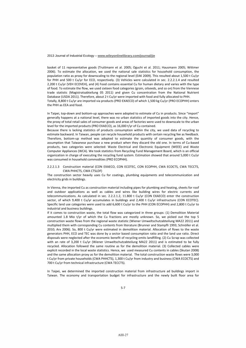
2013 Journal of Industrial Ecology – www.wileyonlinelibrary.com/journal/jie
S 7
basket of 11 representative goods (Truttmann et al. 2005; Oguchi et al. 2011; Hausmann 2005; Wittmer2006). To estimate the allocation, we used the national sale statistics for household consumption, thepopulation ratio as proxy for downscaling to the regional level (EAK 2009). This resulted about 1,500 t Cu/yrfor PHH and 500 t Cu/yr for ECO, respectively. (3) Vehicles were calculated in sec. 2.2.2.1.4 and resulted2,200 t Cu/yr (VEH ECOVEH), and (4) Food contains essential Cu for human dietary and varies with the typeof food. To estimate the flow, we used sixteen food categories (grain, oilseeds, and so on) from the Viennesetrade statistic (Magistratsabteilung 05 2011) and given Cu concentration from the National NutrientDatabase (USDA 2011). Therefore, about 2 t Cu/yr were imported with food and fully allocated to PHH.Totally, 8,800 t Cu/yr are imported via products (PRO EXAECO) of which 1,500 kg Cu/yr (PRO ECOPHH) entersthe PHH as EEA and food.
In Taipei, top down and bottom up approaches were adopted to estimate of Cu in products. Since “import”generally happens at a national level, there was no urban statistics of imported goods into the city. Hence,the proxy of total retail sales of consumer goods and areas of factories were used to downscale to the urbanlevel for the imported products (PRO EXAECO), as 16,000 t/yr of Cu contained.Because there is lacking statistics of products consumption within the city, we used data of recycling toestimate backward. In Taiwan, people can recycle household products with certain recycling fee as feedback.Therefore, bottom up method was adopted to estimate the quantity of consumer goods, with theassumption that Taiwanese purchase a new product when they discard the old one. In terms of Cu basedproducts, two categories were selected: Waste Electrical and Electronic Equipment (WEEE) and WasteComputer Appliances (WCA). We took statistics from Recycling Fund Management Board, which is an officialorganization in charge of executing the recycling fund system. Estimation showed that around 5,000 t Cu/yrwas consumed in household commodities (PRO ECOPHH).
2.2.2.1.3 Construction material (CON EXAECO, CON ECOTEC, CON ECOPHH, CWA ECOCTS, CWA TECCTS,CWA PHHCTS, CWA CTSLDF)
The construction sector heavily uses Cu for coatings, plumbing equipments and telecommunication andelectricity grids in buildings.
In Vienna, the imported Cu as construction material including pipes for plumbing and heating, sheets for roofand outdoor applications as well as cables and wires like building wires for electric currents andtelecommunications. As calculated in sec. 2.2.2.1.2, 11.800 t Cu/yr (CON EXAECO) enter the constructionsector, of which 9,400 t Cu/yr accumulates in buildings and 2,400 t Cu/yr infrastructure (CON ECOTEC).Specific land use categories were used to add 6,600 t Cu/yr to the PHH (CON ECOPHH) and 2,800 t Cu/yr toindustrial and business buildings.If it comes to construction waste, the total flow was categorized in three groups: (1) Demolition Materialamounted 1.8 Mio t/yr of which the Cu fractions are mostly unknown. So, we picked out the top 5construction waste flows from the regional waste statistic (Wiener Umweltschutzabteilung MA22 2011) andmultiplied them with corresponding Cu contents from literature (Brunner and Stampfli 1993; Schnöller et al.2010; Arx 2006). So, 800 t Cu/yr were estimated in demolition material. Allocation of flows to the wastegenerators PHH, ECO and TEC was done by a sector based consumption ratio and the land use ratio. Directdisposals were neglected after the economic benefit of recycling omits landfilling. (2) Cu Scrap was collectedwith an rate of 3,200 t Cu/yr (Wiener Umweltschutzabteilung MA22 2011) and is estimated to be fullyrecycled. Allocation followed the same routine as for the demolition material. (3) Collected cables wereexplicit recorded in the local waste statistics. Hence, we used measured Cu contents in cables (Skutan 2008)and the same allocation proxy as for the demolition material. The total construction waste flows were 3,000t Cu/yr from private households (CWA PHHCTS), 1,300 t Cu/yr from industry and business (CWA ECOCTS) and700 t Cu/yr from technical infrastructure (CWA TECCTS).
In Taipei, we determined the imported construction material from infrastructure ad buildings import inTaiwan. The economy and transportation budget for infrastructure and the newly built floor area for
AIII-27

2013 Journal of Industrial Ecology – www.wileyonlinelibrary.com/journal/jie
S 8
buildings were included to downscale statistics from Taiwan to Taipei. The two categories contributed to45.3% of the total Cu consumed in Taipei which was 13,000 t/yr (CON EXAECO).We allocated the imported construction material to construction material consumption in economic sectors,private households and infrastructure by the proportion of land use area. Cu consumed in households andinfrastructure was then estimated to be 8,000 t/yr (CON ECOPHH) and 4,000 t/yr (CON ECOTEC),respectively.For construction waste, construction and demolition waste (C&D waste) and total demolished floor area ofthe year were considered. Allocation for households, infrastructure an economy sectors were determined bythe corresponding area of land use in Taipei. Results show that Cu in construction waste are 150 t/yr fromprivate households (CWA PHHCTS), 50 t/yr from infrastructure (CWA TECCTS) and 3 t/yr from economysectors (CWA ECOCTS). The relatively low amount of construction waste produced from infrastructure andeconomy sectors may be due to the longer lifespan of the infrastructure and buildings.
2.2.2.1.4 Vehicles (VEH ECOVEH, WAS VEHCTS, VEH UID, VEH VEHECO)Cu is extensively used in vehicles and rolling stocks. It is part of electrical components, heat transfer devices,and bronze sleeve bearings. Hence, countless fittings, fasteners, and screws are made from brass (EuropeanCopper Institute (ECI) 2011).
In Vienna, the modal split in the traffic sectors allocates 1/3 of all trips to public transport, 1/3 to private carsand 1/3 to non motorized traffic like cycling and walking. So, private and public transport fleets are of equalimportance for Cu calculations. To estimate the inflow, we used official registration statistics for vehicles likecars, busses, lorries and motor bikes (Statistik Austria 2008), the rolling stock alteration of the publictransport provider (Lebhart 2010), and the and the average Cu content per vehicle found in the literature(European Copper Institute (ECI) 2011; Bertram et al. 2002; Struckl 2007). This results an inflow of 2,200 tCu/yr (VEH ECOVEH). The total outflow has not been statistically reported. So, the whereabouts of EOL carscan’t be determined at full scale. We carried out a national car balance in order to estimate the number ofunidentified cars. Hence, the Viennese car ownership of 15.3% acts as proxy for regional scaling (StatistikAustria 2008) and an average Cu content per car was used to estimate Cu flows. This results an outflow of880 t Cu/yr of which 240 t Cu/yr enter a shredder (WAS VEHCTS), 140 t Cu/yr t are legally exported to foreigncountries (VEH VEHECO) and 500 t Cu/yr remain unidentified in terms of their whereabouts (VEH UID).
In Taipei, private vehicles dominate transportation, especially the sedans and scooters. Since statistics ofnewly sold vehicles were absent, Cu estimation was top down from the national data. Vehicles which areready to be in use were assumed to be the sales volume of cars and scooters/motorcycles of the study year.By the Taipei Taiwan ratio of newly registered vehicles and Cu content 1.4% (Bertram et al. 2002), salesvolumes in Taipei was estimated to be 500 t/yr of Cu (VEH ECOVEH).We assumed that all end of life vehicles (ELV) were treated as recyclable waste. Since data of recycled ELV inTaipei was lacking, we used statistics of recycled ELV in Taiwan and Taipei Taiwan ratio of newly registeredvehicles to top down the estimation, as a result of 200 t/yr of Cu in waste vehicles (WAS VEHCTS).Amount of registered vehicles difference between 2008 and 2009 was assumed to be the exported ELV,since the change of ELV was unknown and unclear. Hence, 90 t Cu/yr in ELV (VEH VEHECO) was estimated toleave the city boundary.
2.2.2.1.5 Particulate emissions (PAE VEHTEC, PAE VEHPBL, PAE TECPBL)Particulate emissions are driven by wearing, weathering and corrosion processes. Diffuse emission patternsare characteristic for urban areas. They end up in urban soil and surface runoff.
In Vienna, we considered three main emission sources. First, brake wears from low duty vehicles wasestimated according to the fleet mileage (Holzapfel and Riedel 2011), average total wear rates (Winther andSlento 2010) and Cu concentrations in brake linings representing the Austrian fleet (Figi et al. 2010). Finallywe used transfer coefficients from the Netherlands National Emission Inventory (Hulskotte et al. 2006; Oonket al. 2005) in order to examine the flows towards ambient air, road surfaces and vehicle depositions.
AIII-28
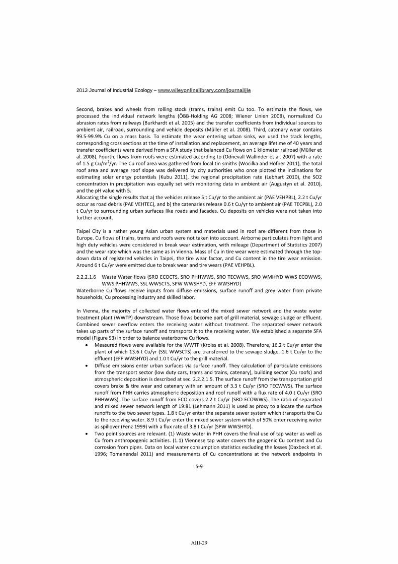
2013 Journal of Industrial Ecology – www.wileyonlinelibrary.com/journal/jie
S 9
Second, brakes and wheels from rolling stock (trams, trains) emit Cu too. To estimate the flows, weprocessed the individual network lengths (ÖBB Holding AG 2008; Wiener Linien 2008), normalized Cuabrasion rates from railways (Burkhardt et al. 2005) and the transfer coefficients from individual sources toambient air, railroad, surrounding and vehicle deposits (Müller et al. 2008). Third, catenary wear contains99.5 99.9% Cu on a mass basis. To estimate the wear entering urban sinks, we used the track lengths,corresponding cross sections at the time of installation and replacement, an average lifetime of 40 years andtransfer coefficients were derived from a SFA study that balanced Cu flows on 1 kilometer railroad (Müller etal. 2008). Fourth, flows from roofs were estimated according to (Odnevall Wallinder et al. 2007) with a rateof 1.5 g Cu/m2/yr. The Cu roof area was gathered from local tin smiths (Wocilka and Höfner 2011), the totalroof area and average roof slope was delivered by city authorities who once plotted the inclinations forestimating solar energy potentials (Kubu 2011), the regional precipitation rate (Lebhart 2010), the SO2concentration in precipitation was equally set with monitoring data in ambient air (Augustyn et al. 2010),and the pH value with 5.Allocating the single results that a) the vehicles release 5 t Cu/yr to the ambient air (PAE VEHPBL), 2.2 t Cu/yroccur as road debris (PAE VEHTEC), and b) the catenaries release 0.6 t Cu/yr to ambient air (PAE TECPBL), 2.0t Cu/yr to surrounding urban surfaces like roads and facades. Cu deposits on vehicles were not taken intofurther account.
Taipei City is a rather young Asian urban system and materials used in roof are different from those inEurope. Cu flows of trains, trams and roofs were not taken into account. Airborne particulates from light andhigh duty vehicles were considered in break wear estimation, with mileage (Department of Statistics 2007)and the wear rate which was the same as in Vienna. Mass of Cu in tire wear were estimated through the topdown data of registered vehicles in Taipei, the tire wear factor, and Cu content in the tire wear emission.Around 6 t Cu/yr were emitted due to break wear and tire wears (PAE VEHPBL).
2.2.2.1.6 Waste Water flows (SRO ECOCTS, SRO PHHWWS, SRO TECWWS, SRO WMIHYD WWS ECOWWS,WWS PHHWWS, SSL WWSCTS, SPWWWSHYD, EFF WWSHYD)
Waterborne Cu flows receive inputs from diffuse emissions, surface runoff and grey water from privatehouseholds, Cu processing industry and skilled labor.
In Vienna, the majority of collected water flows entered the mixed sewer network and the waste watertreatment plant (WWTP) downstream. Those flows become part of grill material, sewage sludge or effluent.Combined sewer overflow enters the receiving water without treatment. The separated sewer networktakes up parts of the surface runoff and transports it to the receiving water. We established a separate SFAmodel (Figure S3) in order to balance waterborne Cu flows.
Measured flows were available for the WWTP (Kroiss et al. 2008). Therefore, 16.2 t Cu/yr enter theplant of which 13.6 t Cu/yr (SSL WWSCTS) are transferred to the sewage sludge, 1.6 t Cu/yr to theeffluent (EFF WWSHYD) and 1.0 t Cu/yr to the grill material.
Diffuse emissions enter urban surfaces via surface runoff. They calculation of particulate emissionsfrom the transport sector (low duty cars, trams and trains, catenary), building sector (Cu roofs) andatmospheric deposition is described at sec. 2.2.2.1.5. The surface runoff from the transportation gridcovers brake & tire wear and catenary with an amount of 3.3 t Cu/yr (SRO TECWWS). The surfacerunoff from PHH carries atmospheric deposition and roof runoff with a flux rate of 4.0 t Cu/yr (SROPHHWWS). The surface runoff from ECO covers 2.2 t Cu/yr (SRO ECOWWS). The ratio of separatedand mixed sewer network length of 19:81 (Lehmann 2011) is used as proxy to allocate the surfacerunoffs to the two sewer types. 1.8 t Cu/yr enter the separate sewer system which transports the Cuto the receiving water. 8.9 t Cu/yr enter the mixed sewer system which of 50% enter receiving wateras spillover (Fenz 1999) with a flux rate of 3.8 t Cu/yr (SPWWWSHYD).
Two point sources are relevant. (1) Waste water in PHH covers the final use of tap water as well asCu from anthropogenic activities. (1.1) Viennese tap water covers the geogenic Cu content and Cucorrosion from pipes. Data on local water consumption statistics excluding the losses (Daxbeck et al.1996; Tomenendal 2011) and measurements of Cu concentrations at the network endpoints in
AIII-29

2013 Journal of Industrial Ecology – www.wileyonlinelibrary.com/journal/jie
S 10
households (Magistratsabteilung 31 2008) result a flux rate of 2.3 t Cu/yr. (1.2) Human off flows likefeces, urine and skin particles result about 760 mg Cu/cap/yr (I C Consultants Ltd 2001; Lampert et al.1997). Other emission sources like residues from food preparation, washing dishes, toilet papers,washing clothes and cleaning activities count for 843 mg Cu/cap/yr (Baccini et al. 1993; I CConsultants Ltd 2001). The multiplication with Viennese population size results 2.7 t Cu/yr. In total,the flux rate is 5.0 t Cu/yr (WWS PHHWWS). (2) Waste water data from business and industries wererestricted for access. As a consequence, we calculated the flow by stressing the mass balanceprinciple with a flux rate of 7.4 t Cu/yr (WWS ECOWWS).
Figure S3: Cu in urban water flows (Diffuse emissions = yellow, Point emissions = pink, Outputs fromWWS =blue)
In Taipei, the percentage of houses connected to public sanitary sewers is 100%. There are threewastewater treatment plants in operation for Taipei: Dihua, Neihu, and Bali. Local statistics showed that Cuin untreated and treated wastewater from Neihu WWTP were not detectable (< 0.02 mg/L). To estimate theflow, we set the detection limit of 0.02 mg Cu/l as maximum concentration. The estimation turned out to be9.8 t/yr (WWA PHHWWS) and 2.8t/yr (TWA WWSHYD). By the ratio of different land uses, Cu in surfacerunoff was 0.02 t/yr (SRO ECOWWS), 0.5 t Cu/yr (SRO PHHWWS) and 0.4 t Cu/yr (SRO TECWWS). Cu insewage sludge was then estimated to be 60 t Cu/yr (SSL WWSCTS). To estimate the flow, we used thesewage sludge flow with 65,700 tons (sum of Bali, Dihua, and Neihu sewage farms) and Cu concentrationswith 887 ppm from Bali Sewage Farm (Shih 2007).
2.2.2.1.7 Solid waste (HHW PHHCTS, WAS ECOCTS)Cu in solid waste streams are much sought after by stockholders in the recycling and recovering business.Due to the economic incentivizes waste collection strategies and technologies that gain valuable metals arecontinuously improved.
In Vienna, waste from private households, industry and business covered four waste streams: (1) Municipalsolid waste and likewise fractions from business and industry was collected by public service providers. Itamounts 579,888 t/yr, while recent studies in Austria determine the concentration from 1,800 – 2,200 mgCu/kg (Skutan and Rechberger 2007). (2) Waste from industry and business contains four industrial wastefractions like waste from punching and planking, Cu chloride, non ferrous metal scrap and electroplatingsludge. To estimate the flow, we used local waste statistics (Wiener Umweltschutzabteilung MA22 2011) andwaste specific Cu contents derived from personal correspondence (Daxbeck et al. 2006). (3) Bulky wastecomposition varies all over Austria due to different collection schemes. In Vienna, about 70.000 t arecollected as composite materials, wood and metals (Wiener Umweltschutzabteilung MA22 2011). After theCu content is varying to a large extent, we used a broad bandwidth from 1,800 3,300 mg/kg (Skutan andBrunner 2006). (4) Waste electrical and electronic equipment (WEEE) covers large apparatuses, fridges, andfreezers, monitors, small WEEE and lamps. To estimate the Cu flow from private households, we usedcollection data from the national coordination center for WEEE and Cu concentrations from a Swiss Cu flow
Waste Water System WWS
AIII-30

2013 Journal of Industrial Ecology – www.wileyonlinelibrary.com/journal/jie
S 11
study (Wittmer 2006). Those from business were not exclusively reported for Vienna. Therefore, the nationalamount was downscaled by the ratio of WEEE from private households to total WEEE flow in Vienna.Summarizing, about 1,700 t Cu/yr were generated by households (HHW PHHCTS) and 5,400 t Cu/yr byindustry and business (WAS ECOCTS).
In Taipei, household waste includes the trash collected by cleaning squad and by people themselves, as wellas the recyclables. Result shows that 1,700 t/yr of Cu contained in household waste (HHW PHHCTS). InTaiwan, industrial waste comprises from industries and service sectors. Since there was nearly no factory inTaipei, industrial waste was presumed to come from service sectors, whose composition is similar tohousehold waste. Because the process ECO was defined as the industrial sector, the amount of industrialwaste transported by industrial or waste management institutes to incinerators and landfill sites wereconsidered. Cu concentration in industrial waste was assumed to be as the same as bottom ash and fly ashfrom incinerators with a rate of 60 t Cu/yr (WAS ECOCTS).
2.2.2.1.8 Exported products (PRO ECOEXA)Exported products stand for valuable goods which cross the city boundary.
In Vienna, exported products cover three sub flows. First, the exported vehicles are traded as goods andwere estimated to be 140 t Cu/yr (VEH VEHECO). Second, the number of unregistered EOL vehicles wasassumed to be exported with 500 t Cu/yr (VEH UID). Third, fabricated goods from the production industrylack of sound data after the import/export statistics are based on the headquarter approach instead of aterritorial allocation. So, we estimated 2,000 t Cu/yr with the help of import/export statistics and subtractedresidues from production. In total, 2,600 t Cu/yr leave Vienna in a physical product form (PRO ANTEXA).
In Taipei, the same estimation assumption was made as in Vienna, and products exported from Taipei Citywere estimated to be 8,000 t Cu/yr.
2.2.2.1.9 Exported waste including recyclables (WAS CTSEXA)Exported waste flows are directed to recycling or disposal facilities out of the city. They cover valuable Cuwhich is recovered as well unrecovered Cu in residues from incineration.
In Vienna, we combined the generated waste flows, individual information regarding the whereabouts inrecycling facilities and specific Cu contents. The flow is summarized by individual flows like recyclables withinconstruction waste, waste from industry and business, and recycled EOL vehicles to an extend of 11,100 tCu/yr (WAS CTSEXA).
Taipei City incinerated household waste from Keelung City too and stored the bottom ash temporarily duringthe period of constructing new landfill in Keelung. Likewise, Keelung City would provide landfill service ofwaste from Taipei City and temporary depository fly ash monolith. The temporary repository of bottom ashand fly ash will be sent back to the original city after the new landfill is constructed. Statistics of Taipei Cityshowed that in 2003 total weight of bottom ash conveyed to Keelung City was 96,000 tons. We also assumedthat ELV, scrap, and recyclables were included in exported waste, result in total 2,700 t Cu/yr (WAS CTSEXA).
2.2.2.1.10 Incineration: Mixed waste, exported residues for underground storage, residues, disposablewaste (WAS CTSINC, TTR INCEXA, RES INCLDF)
Waste incinerators are used to treat household and toxic industrial waste by temperatures up to 1,200 °C.While microorganisms like bacteria, fungi and virus as well as organic compounds are mineralized, heavymetals like Cu are transferred to bottom ash and APC residues. The whereabouts of residues depends onnational polices and varies from bottom ash as construction material to underground disposal for filter APCresidues.
AIII-31

2013 Journal of Industrial Ecology – www.wileyonlinelibrary.com/journal/jie
S 12
In Vienna, four plants secure the treatment of household waste, residues from mechanical sorting, bulkywaste fractions, street litter and some minor waste fractions with an amount of 600,000 t/yr. To estimatethe plant load, we used Cu concentrations for six different waste flows that stem from plant specificmonitoring reports and waste flow measurements (Boller 2002; Skutan and Brunner 2006; Skutan andRechberger 2007; Umweltbundesamt 2000; Arx 2006; Hausmann 2005). Therefore, about 1,140 t Cu/yrenter the incinerators (WAS CTSINC). Public secondary waste flow data (Wiener UmweltschutzabteilungMA22 2011) and measured Cu concentrations in a representative Austrian waste to energy plants (Skutanand Rechberger 2007; Taverna et al. 2011) result 990 t Cu/yr in bottom ash (RES INCLDF) and 16 t Cu/yr inAPC residues (TTR INCEXA). The bottom ash is used as aggregate to construct concrete blocks for landfillstabilization that ends up at a Viennese landfill. APC residues are heavily contaminated with salts and heavymetals. In 2008, they were exported to Heilbronn, an underground storage facility in Germany.
In Taipei, three incinerators operate for Taipei: Beitou, Neihu, and Muzha. According to local statistics, wastetransported into incinerator was 640,000 ton in 2009. Cu content was estimated from the Cu concentrationin fly ash and bottom ash. Cu in municipal solid waste (MSW) was 200 t/yr (WAS CTSINC). Residues fromincinerators consist of fly ash and bottom ash, which contained 200 t/yr of Cu (RES INCLDF). Due to thepolicy “Zero Waste” of the local government, the waste amount in Taipei has decreased, and no statisticsshowed that residues from incinerators were exported from the city. Hence, Cu in exported residue forunderground storage is zero (TTR INCEXA) in Taipei’s case.
2.2.2.1.11 Composting: Compostable waste, residues, compost as fertilizer (WAS CTSCOM, RES COMCTS,COM COMUPV)
Composting degrades biogenic waste in terms of volume and mass. Quality proven compost can be used asnutrient supplier for plants and soil improver.
In Vienna, one compost plant has been operated. The inputs stem from separated biomass collection andcover materials such as greencut and uncooked vegetables from households. To estimate the Cu flowsthroughout the plant, we used monitored bulk flows, and derived average dry matter contents as well as Cuconcentrations from the literature. The inflow covers compostable raw materials and residues fromanaerobic digestion in a biogas plant (Magistratsabteilung 48 2009). Data lacks prevented full Cu balance onplant level. So we set the output as net addition to plant. We assumed a dry matter ratio of 30% and a Cuconcentration of 83 mg/kg dry matter and results 1.4 t Cu/yr (WAS CTSCOM). About 33.000 t valuablecompost is used for land applications in Vienna (Republik Österreich 2001b; Weinmar 2011). Legal Cuconcentrations for high quality compost A+ was set with 70 mg/kg dry substance (Republik Österreich2001a) and resulted 1.4 t Cu/yr (COM CTSCOM = COM COMUPV).
In Taipei, incinerator plants in Taipei have auxiliary spaces to process compost, which has nothing to do withincinerators themselves. Uncooked food waste scraps are collected to incinerator plants and through theprocess of dehydration, fermentation, etc., they become compost as product. People or companies can takethe compost if they need. Since there are few livestock industries or agricultural activities in Taipei, thecompost here was assumed to be the treated uncooked food waste without residues. Due to limited data,the official statistics of uncooked food waste scraps in Taipei City and compost from Muzha RefuseIncineration Plant were adopted to estimate total compost in Taipei, which included 0.04 t Cu/yr (WASCTSCOM, COM COMUPV).
2.2.2.1.12 Pesticides (PES ECOUPV)The agricultural sector applies Cu as purposeful fungicides and bactericide on fruits and vegetables. Theutilization of Cu dates back to beginning of the 19th century and was known as “Bordeaux Brühe” It is amixture of chalk and aquatic Cu sulphate dissolution and bans the evolution of mildew. In 2009, theEuropean Commission decided to constrain Cu form agricultural appliances after 2016 (Berger et al. 2011).Member states are enforced to establish national risk assessments in order to regulate Cu use.
AIII-32

2013 Journal of Industrial Ecology – www.wileyonlinelibrary.com/journal/jie
S 13
In Vienna, the flow was calculated based on data on Austrian pesticide and plant protection product use(Berger et al. 2011) for wine, fruits and vegetables & crops and Viennese agricultural land use areas. In total,about 2.4 t Cu/yr are released by pesticides (PES ECOUPV).
In Taipei, there are barely agricultural activities; the agricultural area is 5.31 km2, which is around 2% of totalarea of the city. Hence, estimation of Cu in pesticides was not included for Taipei’s case.
2.2.2.1.13 Fertilizer (FER ECOUPV)Manure, mineral fertilizer and harvest residues are common fertilizer inputs into agricultural soils. Especiallymanure is known to have a significant Cu concentration. Concentrations vary from 40 300 mg Cu/kg manuredepending on the type of animal and foodstuff (Zethner et al. 2007). As an example, Cu is given to piglets inhigh doses to protect them from various diseases in the first weeks. Mineral fertilizer and harvest residuescover minor Cu as trace element.
In Vienna, the agricultural sector plays a minor role in terms of land use and production rates. About 15% ofurban area is used to produce working animals, crops, wine and vegetables for local supply primarily. The Curelease was estimated by multiplying normalized Austrian and German Cu inputs (Fricke and Höhl 2000;Umweltbundesamt 2001; Zethner et al. 2007; Berger et al. 2011) with agricultural area classified intoviticulture production, fruit production, and agriculture & horticulture (Fitzthum 2009). In total about 2.2 tCu/yr are released by fertilizer applications (FER ECOUPV).
In Taipei, there are barely agricultural activities; the agricultural area is 5.31 km2, which is around 2% of totalarea of the city. Hence, estimation of Cu in fertilizer was not included for Taipei’s case.
2.2.2.1.14 Technical Infrastructure (TECstock)Cu is mainly used for electricity transmission and information transfer.
In Vienna, three types of networks are taken into account. First, the electricity grid covers ~3.700 km ofoverhead lines and ~ 22.300 km of underground cables (Wien Energie 2010). The stock was estimated basedon voltage classes, cable lengths, cross sections and specific masses according to the Swiss network (Wittmer2006). In total, about 89,200 t Cu provide the public energy supply. Second, Cu in the telecommunicationnetwork is estimated by a proxy based on the number of business units. Combining data from Australia andSydney (van Beers and Graedel 2007) with Viennese business statistics resulted about 13,300 t Cu. Third,catenaries supply the 2nd largest tram network worldwide as wells as national and local railway tracks withelectricity. The Cu stock of 1,000 t is estimated based on the track length, cross sections, Cu content, andlifetime data. Summarizing, the infrastructure covered about 103,000 t Cu. In reality, the stock is larger thanestimated due to Cu cables in subway lines and power transfer stations which were not taken into account.
In Taipei, the electricity transmission system and telecommunication system were taken into account. Theelectricity grid included 2,100 km overhead power lines and 310 km underground power lines (Lin 2003). Forthe telecommunication network, estimation was made according to case of Australia and statistics ofhousehold and business number in Taipei which gave a result of 24,000 t Cu. Cu stock in infrastructure wasaggregated as 32,000 t Cu. Since Cu stock in cables and wires of MRT (Mass Rapid Transit) was not included,the actual value stock maybe larger than the estimated one.
2.2.2.1.15 Economy and private households (ECOstock, PHHstock)The process economy and private household covers stocks like roofs, water pipes, heating systems,telecommunication and electricity networks as well as consumer goods.
AIII-33

2013 Journal of Industrial Ecology – www.wileyonlinelibrary.com/journal/jie
S 14
In Vienna, the building structure and housing technology is comparable to Swiss standards. Using per capitadata from Switzerland (Wittmer 2006) result about 134,000 t Cu in buildings. The land use area is used asproxy to allocate 94,000 t Cu to private households and 40,000 to economy. Cu in consumer goods likewashing machine, dryer, electronics equipment and minor items like keys and coins stands for 37,000 t Cu.They were allocated to private households.
In Taipei, we selected items based on products listed in recycling fund system to estimate Cu stock inconsumer goods. Assumption was made that those Cu contained products included in recycling fund systemwere those comparatively highly used in households in Taiwan. The lifespan of different products werepresumed to be uniform distribution. These consumer goods were either electrical and electronic appliances(EEA) or computer appliances. Five items for Cu stock calculation were color TV, air conditioner, washingmachine, laptop, and desktop computer. With numbers of hundred households in Taipei as 9,628.31 in 2009,Cu consumed annually in household appliances and computer appliances in Taipei City were 17,000 t Cu.In economy sectors (ECO), building materials were assumed to be the stocks in it while consumer productswere all input to private households (PHH). Electricity and telecommunication wire and cables were takeninto account for Cu stock of buildings. In this study, the average length of in use line in a case study in Tainan(Ou et al. 2007) and the total floor area in Taipei were integrated to do estimation. The Tainan case wasreasonable and suitable for estimating because its structure and space usage are common around Taiwan,and hence the case could represent the general housing in Taiwan as well as in Taipei. We used ratio of landuse to allocate Cu stocks of buildings to ECO and PHH. The result shows that 200 t Cu existed in the form ofbuilding materials in ECO.
2.2.2.1.16 Vehicles (VEHstock)The vehicle pool covers private and commercial wheelers as well as rolling stocks.
In Vienna, the calculation is based on the number of vehicles (Statistik Austria 2008; Wiener Linien 2009) andcorresponding Cu contents from literature (Bertram et al. 2002; European Copper Institute (ECI) 2011; Hoock2008; Struckl 2007). The private and public owned fleet consist registered motorized vehicles like cars,lorries and busses as well as rolling stock such as subways and trams. In total, the Cu stock in the transportsector covers 24.000 t Cu.
In Taipei, the estimation included the number of registered cars, buses and scooters in operation. 12,000 tCu was estimated to be placed in vehicles.
2.2.2.1.17 Urban Soil (UPVstock)Urban soil covers Cu, which compromises geogenic backgrounds and former anthropogenic inputs.
In Vienna, soil sampling data were reported by the City Authority. We printed a box plot including thedetected Cu concentrations in parks and playgrounds. Therefore, about 46 mg Cu/kg soil were multipliedwith the area of green space and a soil depth of 30 cm. This results about 4,000 t Cu in urban soil (UPVstock).
In Taipei, there is no local report of the soil sampling data, and hence estimation was made according to EPApublic health declaration that Cu concentration in soil generally ranges from 2 to 250 ppm. With the area ofgreen space of Taipei City and 30 cm depth of soil, Cu stock in urban pedosphere was obtained to be 830 t(UPVstock).
AIII-34

2013 Journal of Industrial Ecology – www.wileyonlinelibrary.com/journal/jie
S 15
2.2.2.2 Vienna – List of mathematical model equations and input parameters
Table S3: Model Equations and flow resultsFlow Acronym Description Equation Expected
Value[t/yr]
Deviation[t/yr]
01 ADE PBLECO Atmospheric Deposition ECO Dep * AECO 1.1 0.1902 ADE PBLPHH Atmospheric Deposition PHH Dep * APHH 1.5 0.2603 ADE PBLTEC Atmospheric Deposition TEC Dep * ATEC 0.9 0.1504 ADE PBLUHY Atmospheric Deposition UHY Dep * AUHY 0.3 0.0505 ADE PBLUPV Atmospheric deposition UPV Dep * AUPV 2.8 0.4806 COM ANTUPV Compost, applied on land mcomp * wcomp * ccomp 1.4 0.2407 CON ECOPHH Construction Material ConsAUT* ProxyMarket Share* Proxy Employees, bui * Proxyarea 6,567 938
08 CON ECOTEC Construction material ConsAUT* ProxyMarket Share* Proxy Employees, bui 2,448 376
09 CON EXAECO Imported construction material ConsAUT* ProxyMarket Share* Proxy Employees, bui 11,817 1,390
10 CWA ECOCTS Construction waste ECODemolition waste (DEM)Scrap metal (SCR)Cables (Cab)
DEM+SCR+CABDEM=Dem*cdem* (1 Proxyarea)SCR= Scrab*cscrabl * Proxypre products, scrap * (1Proxyarea)CAB=Cable*ccable * Proxypre products, cable * (1Proxyarea)
1,275223894158
21753
20737
11 CWA PHHCTS Construction waste PHH DEM+SCR+CABDEM=Dem*cdem * ProxyareaSCR= Scrab*cscrabl * Proxypre products, scrap * ProxyareaCAB=Cable*ccable * Proxypre products, cable * Proxyarea
2,983522
2,092369
50912348686
12 CWA TECCTS Construction waste TEC DEM+SCR+CABDEM=Dem*cdemSCR= Scrab*cscrabl * Proxypre products, scrap
CAB=Cable*ccable * Proxypre products, cable
68290
249343
107146286
13 EFF WWSHYD Effluents mcu, inflow * TCcu, WWTP 1.6 0.1214 FER ECOUPV Fertilizer Aagr *mfertilizer 2.2 0.315 HAR UPVECO Harvest muptake * ProxyLand use, agriculture 0.3 0.0516 HHW PHHCTS Household waste
Municipal Solid Waste (MSW)Bulky Waste (BW)WEE
MSW+BW+WEEMSW= mMSW* cMSW
BW=mBW * cBWWEE=mWEE, PHH * cWEE
1,6931,123170400
100793452
17 PAE TECPBL Particulate emissions ltrain, tram* ACAT * 1/aCAT * Aloss* TCMOV, TEC 0.6 0.218 PAE VEHPBL Particulate emissions
Low Duty Vehicles (LDV)Rolling Stock (ROL)
LDV+ROLLDV=mil * eLDV* cbrake * TCMOV, TEC
ROL=( ltrain + ltram ) * eROL * TCMOV, TEC
5.04.90.1
2.52.40.3
19 PAE VEHTEC Particulate emissions LDV+ROLLDV=mil * eLDV* cbrake * TCMOV
ROL=( ltrain + ltram ) * eROL * TCMOV
2.22
0.1
1.21
0.620 PES UANUPV Pesticides Aagr* prate 2.4 0.321 PRO ECOEXA Exported products
EOL vehicles for export (VEH VEHECO)Unidentified Vehicles (VEH UID)Fabricated goods from production sector(FG)
VEH VEHECO + VEH UID + FGVEH VEHECO = cardereg_exp * ccarVEH UID = see row 33FG=Impgood Proxyexp_good * Expgood
2,574138498
1,938
74668
330666
22 PRO ECOPHH Consumer goods & foodElectrical and Electronic Appliances (EEA)Food (FOO)
EEA+FOOEEA = EEAPHH * cEEAFOO=Food * cfood
1,4841,482
2
205205
023 PRO EXAECO Imported products
Cu containing goods (CCG)Electrical and Electronic Appliances(EEAtotal)Vehicles (VEH ECOVEH)Food (FOO)
CCG+EEA+VEH ECOVEH+FOOCCG=ConsAUT * ProxyMarket Share* Proxy Employees, ind
EEAtotal= EEAPHH * cEEA * EEAI/E / EEAPHH
VEH ECOVEH=VEH * cvehFOO=Food * cfood
8,8274,6191,9692,237
2
728625325185
0
24 RES INCLDF Residues from incineration mbottom ash * cbottom ash 986 17025 SPWWWSHYD Combined sewer overflow RatioSPW * RatioSST * (SRO TECWWS + SRO PHHWWS
+ SRO ECOWWS)3.8 0.8
26 SRO ECOWWS Surface runoff ECOAtmospheric Deposition PHH (ADEPBLECO)Roof runoff (PAE ECOURS)
ADE PBLECO + PAE ECOURSADE PBLPHH=see row 01PAE PHHURS= AreaRoof * RatioCuroof * rroof * (100ProxyPHH, roof)
2.21.11.1
0.50.190.50
AIII-35

2013 Journal of Industrial Ecology – www.wileyonlinelibrary.com/journal/jie
S 16
27 SRO PHHWWS Surface runoff PHHAtmospheric Deposition PHH (ADEPBLPHH)Roof runoff (PAE PHHURS)
ADE PBLPHH + PAE PHHURSADE PBLPHH=see row 02PAE PHHURS= AreaRoof * RatioCuroof * rroof *ProxyPHH, roof
4.01.52.5
1.30.261.26
28 SRO TECWWS Surface runoff TECAtmospheric Deposition TECBrake & Tire wear on TEC (PAE VEHTEC)Catenary wear on TEC (PAE TECTEC)Street litter (WAS TECCTS)
ADE PBLTEC + PAE MOVTEC + PAE TECTEC WASTECCTS
ADE PBLTEC = see row 03PAE VEHTEC= see row 19PAE TECTEC= ltrain, tram * ACAT * 1/aCAT * Aloss*TCMOV, TEC
WAS TECCTS= see row 40
3.30.92.22.01.8
1.50.21.20.90.05
29 SRO WMIHYD Surface Runoff SRO TECWWS * (1 RatioSST) 1.8 0.0530 SSL WWSCTS sewage sludge mcu, inflow * TCcu, WWTP 13.6 1.131 TTR INCEXA Exported APC residues mAPC res * cAPC res 16.4 1.332 VEH ECOVEH Vehicles, consumed in Vienna Vehicles*cvehicles 2,237 18533 VEH UID Unidentified cars 498 330
34 VEH VEHECO EOL vehicles for export 138 6835 WAS CTSCOM Compostable waste (net addition) mcomp * wcomp * ccomp 1.4 0.336 WAS CTSEXA Exported Waste and Recyclables mWR 11,135 72937 WAS CTSINC Thermal Treated Waste
Mixed waste (MW)Sewage Sludge (SSL)
MW+SSLMW=mmw * cmw
SSL=see row 30
1,1371,12313.6
80801.1
38 WAS ECOCTS Solid waste ECOWaste from industry and business (WIB)WEE
MSW+WIB+BW+WEEWIB=mwib* cwibWEE=mWEE, PHH * cWEE * ProxyWEE, ECO
5,3905,363
27
457457
339 WAS TECCTS street litter mstreet * cstreet 1.8 0.0540 WAS VEHCTS Waste vehicles 235 3942 WWA ECOWWS Wastewater ECO
Unknown sourcesmcu, inflow + SPW WWSHYD SRO URSMSW – WWAPHHWWS
7.4 1.9
41 WWA PHHWWS Wastewater PHHCu in tap water (TAB)Cu in feces, urine, other products (FUO)
TAB + FUOTAB=mtabwater * Losswater * ccu, tabwaterFUO= CapVIE * (cww + cbf)
5.02.32.7
1.51.520.11
Note: t = metric tons per year
Table S4: Model Equations and stock resultsStock Acronym Description Equation Expected
Value [t]Deviation[t]
LDFstock Landfill wasteLDF * cLDF 144,000 61,000PHHstock Private Households
Buildings (BUI_PHH)Consumer Goods (CONS)
BUI+CONSBUI_PHH= stockbui * CapVIE * ProxyareaCONS=conscap * CapVIE
131,00094,00037,000
35,00032,00013,000
RDAstock River Danube Not identifiedTECstock Transport / Energy / Communication Infrastructure
Catenary (CAT)Electricity Grid (EG)Telecommunication (TEL)
CAT+EG+TELCAT= ltrain, tram * ACATEG= gridlenth* cgridTEL=Unit * Cunit
103,0001,00089,00013,000
11,00050
10,1004,100
USTstock Underground Storage Not identifiedECOstock Urban Industry, Business, Services & Forestry / BUI_ECO= stockbui * CapVIE * (1 Proxyarea) 40,000 14,000VEHstock Vehicles VEHstock * cveh_stock 24,000 2,000UPVstock Urban Pedosphere AUPV * tsoil * dsoil * csoil 4,000 1,000Note: t = metric tons per year
Table S5: List of input parameter (non bold=single values, bold=matrices)InputParameter
Description of data Unit Value Uncertaintylevel
Reference Compileddata
CapAUT Inhabitants Austria # 8,347,341 1 (Statistik Austria 2012)CapVIE Inhabitants Vienna # 1,674,909 1 (Lebhart 2010)Dep Deposition Rate g Cu/ha/yr 148,7 2 (Spiegel 2003)A Total City Area ha 41,487 1 (Lebhart 2010)AUHY Urban Hydrosphere (Open Water Bodies) ha 1,933 1 (Lebhart 2010)ATEC Traffic Surface ha 5,981 1 (Lebhart 2010)APHH Residential Area ha 10,267 1 (Lebhart 2010)AECO Public Facilities and production areas ha 4,381 1 (Lebhart 2010)AUPV Green Space Area ha 18,925 1 (Lebhart 2010)
ConsAUT National Cu Consumption in 2006 t Cu/yr =108,000 2 (Daxbeck et al. 2006) Table S7
AIII-36
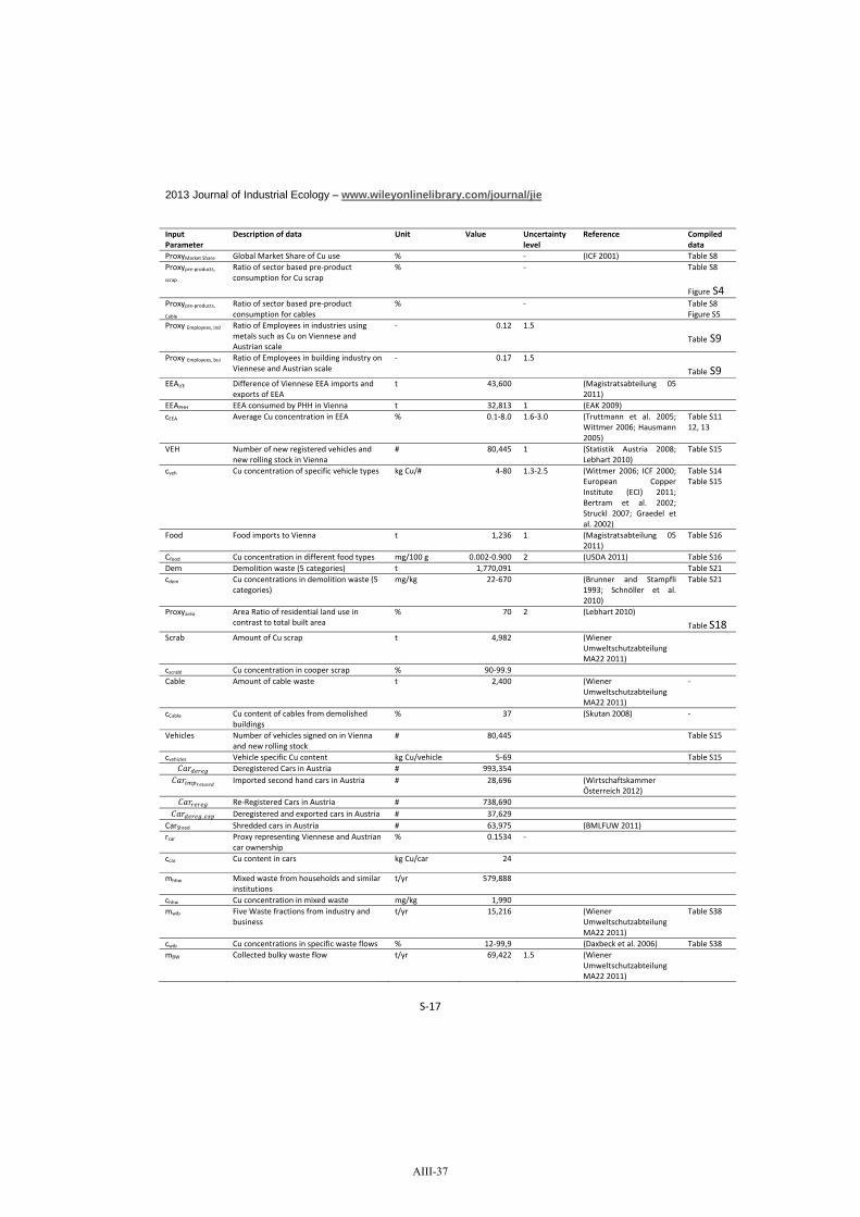
2013 Journal of Industrial Ecology – www.wileyonlinelibrary.com/journal/jie
S 17
InputParameter
Description of data Unit Value Uncertaintylevel
Reference Compileddata
ProxyMarket Share Global Market Share of Cu use % (ICF 2001) Table S8Proxypre products,
scrap
Ratio of sector based pre productconsumption for Cu scrap
% Table S8
Figure S4Proxypre products,
Cable
Ratio of sector based pre productconsumption for cables
% Table S8Figure S5
Proxy Employees, ind Ratio of Employees in industries usingmetals such as Cu on Viennese andAustrian scale
0.12 1.5
Table S9
Proxy Employees, bui Ratio of Employees in building industry onViennese and Austrian scale
0.17 1.5
Table S9EEAI/E Difference of Viennese EEA imports and
exports of EEAt 43,600 (Magistratsabteilung 05
2011)EEAPHH EEA consumed by PHH in Vienna t 32,813 1 (EAK 2009)cEEA Average Cu concentration in EEA % 0.1 8.0 1.6 3.0 (Truttmann et al. 2005;
Wittmer 2006; Hausmann2005)
Table S1112, 13
VEH Number of new registered vehicles andnew rolling stock in Vienna
# 80,445 1 (Statistik Austria 2008;Lebhart 2010)
Table S15
cveh Cu concentration of specific vehicle types kg Cu/# 4 80 1.3 2.5 (Wittmer 2006; ICF 2000;European CopperInstitute (ECI) 2011;Bertram et al. 2002;Struckl 2007; Graedel etal. 2002)
Table S14Table S15
Food Food imports to Vienna t 1,236 1 (Magistratsabteilung 052011)
Table S16
Cfood Cu concentration in different food types mg/100 g 0.002 0.900 2 (USDA 2011) Table S16Dem Demolition waste (5 categories) t 1,770,091 Table S21cdem Cu concentrations in demolition waste (5
categories)mg/kg 22 670 (Brunner and Stampfli
1993; Schnöller et al.2010)
Table S21
Proxyarea Area Ratio of residential land use incontrast to total built area
% 70 2 (Lebhart 2010)
Table S18Scrab Amount of Cu scrap t 4,982 (Wiener
UmweltschutzabteilungMA22 2011)
cscrabl Cu concentration in cooper scrap % 90 99.9Cable Amount of cable waste t 2,400 (Wiener
UmweltschutzabteilungMA22 2011)
cCable Cu content of cables from demolishedbuildings
% 37 (Skutan 2008)
Vehicles Number of vehicles signed on in Viennaand new rolling stock
# 80,445 Table S15
cvehicles Vehicle specific Cu content kg Cu/vehicle 5 69 Table S15Deregistered Cars in Austria # 993,354Imported second hand cars in Austria # 28,696 (Wirtschaftskammer
Österreich 2012)Re Registered Cars in Austria # 738,690Deregistered and exported cars in Austria # 37,629
CarShred Shredded cars in Austria # 63,975 (BMLFUW 2011)rcar Proxy representing Viennese and Austrian
car ownership% 0.1534
ccar Cu content in cars kg Cu/car 24
mhhw Mixed waste from households and similarinstitutions
t/yr 579,888
chhw Cu concentration in mixed waste mg/kg 1,990mwib Five Waste fractions from industry and
businesst/yr 15,216 (Wiener
UmweltschutzabteilungMA22 2011)
Table S38
cwib Cu concentrations in specific waste flows % 12 99,9 (Daxbeck et al. 2006) Table S38mBW Collected bulky waste flow t/yr 69,422 1.5 (Wiener
UmweltschutzabteilungMA22 2011)
AIII-37

2013 Journal of Industrial Ecology – www.wileyonlinelibrary.com/journal/jie
S 18
InputParameter
Description of data Unit Value Uncertaintylevel
Reference Compileddata
cBW Average Cu concentration in bulky waste mg/kg 2,437 2.07 (Skutan and Brunner2006)
mWEE, PHH Collected WEEE in PHH of Vienna t/a 9,044 1 (EAK 2009) Table S40cWEE Cu concentrations of 4 different WEEE
fractions% 1 8 2 5,6 (Wittmer 2006) Table S40
ProxyWEE, ECO Proxy for allocating WEEE to ECO 0.066 (EAK 2009) Table S42
muptake Cu uptake kg Cu/ha/yr 0.01 0.045 (Berger et al. 2011) Table S45ProxyLand use,
agriculture
Agricultural area splitted into differentland use categories
ha =6,281 (Fitzthum 2009) Table S45
prate Pesticide rate kg Cu/ha/yr 0 3.0 2 (Berger et al. 2011) Table S46Aagr Agricultural area splitted into different
land use categories andorganic/traditional farming
ha =6,281 1 (Fitzthum 2009) Table S47
mfertilizer Fertilizer rate kg Cu/ha/yr 0.03 0.55 2 (Fricke and Höhl 2000;Umweltbundesamt 2001;Zethner et al. 2007;Berger et al. 2011)
Table S47
mil Mileage of low duty vehicles in Vienna Veh km 5,694,000,000
(Holzapfel and Riedel2011)
eLDV Total wear rate of brake lining in low dutyvehicles
g /veh km 12.5 (Winther and Slento2010)
cbrake Cu content of brake linings in low dutyvehicles
% 14.231 (Figi et al. 2010, owncalculations to representthe Austrian vehicle fleet)
Table S26
TCVEH, TEC Transfer coefficients describing the ratioof particulate emissions enteringindividual sinks
% (Müller et al. 2008)
Table S25
ltrain Track length of the train network, ownedby National Railway Company ÖBB
track km 761 (ÖBB Holding AG 2008)
ltram Track length of the tram network, ownedby Wiener Linien
track km 363 (Wiener Linien 2008)
eROL Cu abrasion rate of break and wheel wearin trams and trains
g/track km/yr 1,200 (Burkhardt et al. 2005)
lTRAM, TRAIN Track length of train and tram networkaccording to the catenary diameter
track km =1,124 (ÖBB Holding AG 2008;Wiener Linien 2008)
Table S28
ACAT Cross section area of individual catenaries mm 65 120 Table S28aCAT Average lifetime of a catenary yr 40Aloss Average cross section loss over the whole
lifetime% 20
Proxyexp_good Proxy for estimating physical exportsbased on reported flow data (headquarterapproach)
% 50 Assumption
Impgood Imported Cu for producing industries 4,619 see flow PRO EXAECOExpgood Cu waste from production 5,363 see flow WAS ECOCTSmWR Sum of seven Cu waste flows that contain
potential recyclables (demolition material,Cu scrap, cables, waste from industry andbusiness, bulky waste, WEEE, RecycledEOL vehicles)
t/yr =11,071
Table S44
mbottom ash Amount of bottom ash and fly ash t/yr 125,016 1 (WienerUmweltschutzabteilungMA22 2011)
cbottom ash Cu concentration in bottom ash kg Cu/t 7,885 2 (Skutan and Rechberger2007; Mitterbauer et al.2009)
mAPC res Amount of APC residues t/yr 18,189 1 (WienerUmweltschutzabteilungMA22 2011)
cAPC res Cu concentration in APC residues t Cu/t 0.0009011 1.009 (Skutan and Rechberger2007; Taverna et al. 2011)
mcu, inflow Cu Inflow to Waste Water TreatmentPlant
t Cu/yr 16.2 1 (Kroiss et al. 2008)
TCcu, WWTP Transfer Coefficients for Cu in WasteWater Treatment Plant
% 6 85 1 (Kroiss et al. 2008) Table S32
AreaRoof Total Roof Area m² 52.000.000 3 (Kubu 2011)RatioCuroof Percentage of Cu roofs % 5 (Wocilka and Höfner
AIII-38
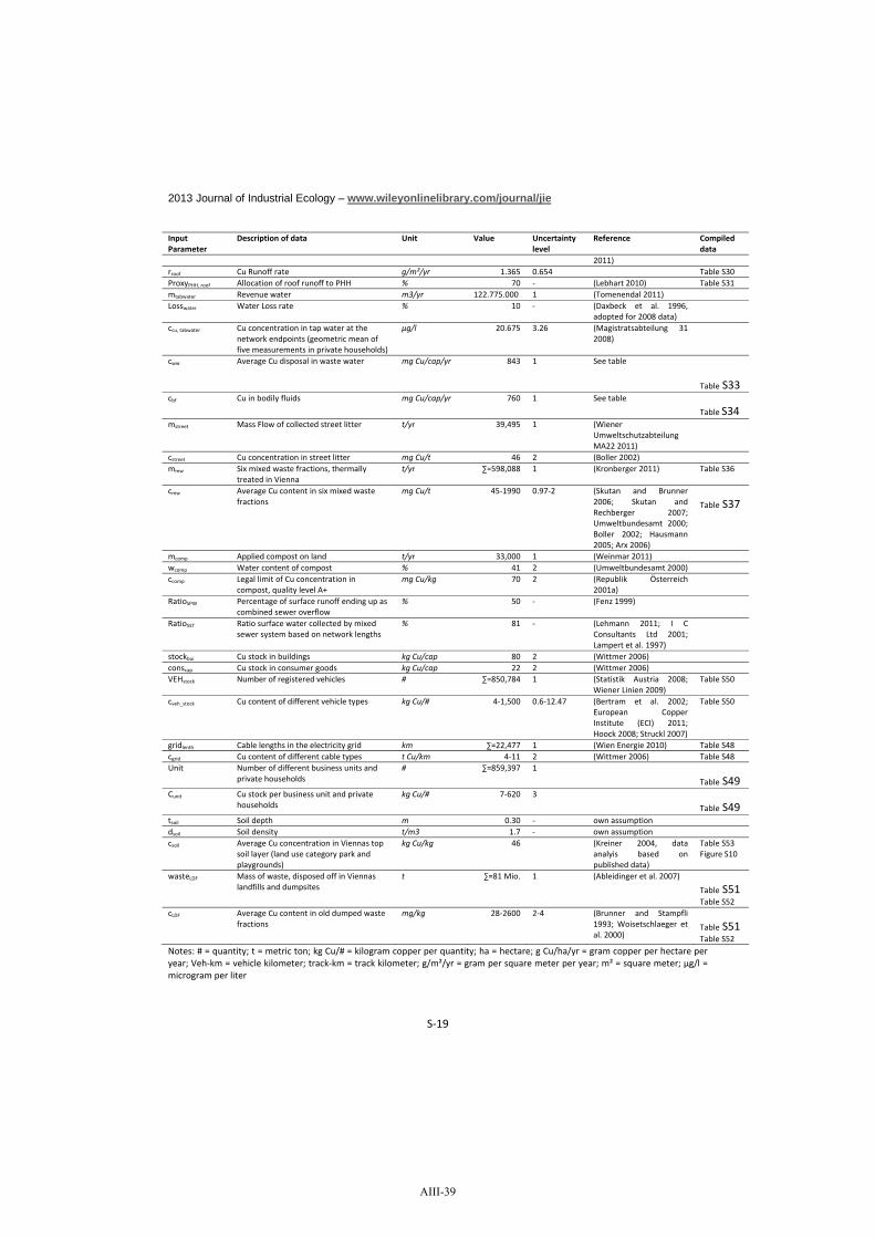
2013 Journal of Industrial Ecology – www.wileyonlinelibrary.com/journal/jie
S 19
InputParameter
Description of data Unit Value Uncertaintylevel
Reference Compileddata
2011)rroof Cu Runoff rate g/m²/yr 1.365 0.654 Table S30ProxyPHH, roof Allocation of roof runoff to PHH % 70 (Lebhart 2010) Table S31mtabwater Revenue water m3/yr 122.775.000 1 (Tomenendal 2011)Losswater Water Loss rate % 10 (Daxbeck et al. 1996,
adopted for 2008 data)ccu, tabwater Cu concentration in tap water at the
network endpoints (geometric mean offive measurements in private households)
μg/l 20.675 3.26 (Magistratsabteilung 312008)
cww Average Cu disposal in waste water mg Cu/cap/yr 843 1 See table
Table S33cbf Cu in bodily fluids mg Cu/cap/yr 760 1 See table
Table S34mstreet Mass Flow of collected street litter t/yr 39,495 1 (Wiener
UmweltschutzabteilungMA22 2011)
cstreet Cu concentration in street litter mg Cu/t 46 2 (Boller 2002)mmw Six mixed waste fractions, thermally
treated in Viennat/yr =598,088 1 (Kronberger 2011) Table S36
cmw Average Cu content in six mixed wastefractions
mg Cu/t 45 1990 0.97 2 (Skutan and Brunner2006; Skutan andRechberger 2007;Umweltbundesamt 2000;Boller 2002; Hausmann2005; Arx 2006)
Table S37
mcomp Applied compost on land t/yr 33,000 1 (Weinmar 2011)wcomp Water content of compost % 41 2 (Umweltbundesamt 2000)ccomp Legal limit of Cu concentration in
compost, quality level A+mg Cu/kg 70 2 (Republik Österreich
2001a)RatioSPW Percentage of surface runoff ending up as
combined sewer overflow% 50 (Fenz 1999)
RatioSST Ratio surface water collected by mixedsewer system based on network lengths
% 81 (Lehmann 2011; I CConsultants Ltd 2001;Lampert et al. 1997)
stockbui Cu stock in buildings kg Cu/cap 80 2 (Wittmer 2006)conscap Cu stock in consumer goods kg Cu/cap 22 2 (Wittmer 2006)VEHstock Number of registered vehicles # =850,784 1 (Statistik Austria 2008;
Wiener Linien 2009)Table S50
cveh_stock Cu content of different vehicle types kg Cu/# 4 1,500 0.6 12.47 (Bertram et al. 2002;European CopperInstitute (ECI) 2011;Hoock 2008; Struckl 2007)
Table S50
gridlenth Cable lengths in the electricity grid km =22,477 1 (Wien Energie 2010) Table S48cgrid Cu content of different cable types t Cu/km 4 11 2 (Wittmer 2006) Table S48Unit Number of different business units and
private households# =859,397 1
Table S49Cunit Cu stock per business unit and private
householdskg Cu/# 7 620 3
Table S49tsoil Soil depth m 0.30 own assumptiondsoil Soil density t/m3 1.7 own assumptioncsoil Average Cu concentration in Viennas top
soil layer (land use category park andplaygrounds)
kg Cu/kg 46 (Kreiner 2004, dataanalyis based onpublished data)
Table S53Figure S10
wasteLDF Mass of waste, disposed off in Viennaslandfills and dumpsites
t =81 Mio. 1 (Ableidinger et al. 2007)
Table S51Table S52
cLDF Average Cu content in old dumped wastefractions
mg/kg 28 2600 2 4 (Brunner and Stampfli1993; Woisetschlaeger etal. 2000)
Table S51Table S52
Notes: # = quantity; t = metric ton; kg Cu/# = kilogram copper per quantity; ha = hectare; g Cu/ha/yr = gram copper per hectare peryear; Veh km = vehicle kilometer; track km = track kilometer; g/m²/yr = gram per square meter per year; m² = square meter; μg/l =microgram per liter
AIII-39

2013 Journal of Industrial Ecology – www.wileyonlinelibrary.com/journal/jie
S 20
2.2.2.3 Vienna Background data
2.2.2.3.1 Products (PRO EXAECO)
2.2.2.3.1.1 OverviewFour groups of products are estimated to represent more than 90% of Cu in imported products:
1. Cu containing goods (Sheet metal, Wires, Cables, Pipes, Pre Products etc.)2. Electrical and electronic appliances3. Vehicles4. Food
Table S6: Imported products (PRO EXAECO)
GoodsFlux rate Deviation
Allocation toECO
Allocation toVEH
Allocation toPHH
[t Cu/yr] [t Cu/yr]
Cu containing goods 4,619 625 4,619
Electrical and Electronic Appliances 1,969 287 486 1,482
Vehicles 2,237 185 2,237
Food 2 0.25 2
Sum 8,827 341 5,105 2,237 1,484
Note: t Cu/yr = metric tons copper per year; ECO = Industry, business, services and forestry; VEH = Vehicles; PHH = PrivateHouseholds
2.2.2.3.1.2 Cu containing goods
Table S7: Cu consumption in Austria (Daxbeck et al. 2006)
N° Austrian Cu ConsumptionFlux rate
[t/yr]1 Electrical conductors, cables 33,0002 Pipes 26,0003 Sheets 15,0004 Wires, Cables, Ropes 12,0005 Rest 22,000
Sum of Cu consumed in Austria 108,000Note: t/yr = metric tons per year
Table S8: Proxy: Cu Market share (ICF 2001)
Global Cu Consumption
Cables &Wires
Pre productCu
Pre productCu Alloy
[%] [%] [%] [%]
Building Sector [%] 20 12 8 40
Infrastructure [%] 13 1 1 15
Other Production Industries [%] 19 7 19 45
Total Product Share 52 20 28 100
AIII-40

2013 Journal of Industrial Ecology – www.wileyonlinelibrary.com/journal/jie
S 21
Table S9: Proxy: Employees
Austria Vienna ProxyReference
[#] [#] []
Employed people in buildingindustry
275,266 46,736 0.17(Statistik Austria 2009c; Hauptverband
der österreichischenSozialversicherungsträger SV 2011)
Employed people in industriesusing metals such as Cu (ÖNACE2008 C24 C30 and C33)
345,926 42,081 0.12
Note: # = quantity
Table S10: Vienna Cu consumption by sector: Downscaling and allocation of Cu consumptionAustria Vienna
Cables & Wires[t Cu/yr](1)+(4)
Pre product[t Cu/yr](2)+(3)+(5)
Sum [tCu/yr]
Proxy:Employees
CablesandWires[t/yr]
Pre product[t Cu/yr]
Sum [tCu/yr]
Allocation toflow
Note
Building Sector17,308 37,800 55,108 0.17 2,942 6,426 9,368 CON EXAECO
Followsec. 2.2.2.1.3
Infrastructure11,250 3,150 14,400 0.17 1,913 536 2,449 CON EXAECO
Followsec. 2.2.2.1.3
Other producingIndustries
16,442 22,050 38,492 0.12 1,973 2,646 4,619 PRO EXAECO
SUM 45,000 63,000 108,000 6,828 9,608 16,436
Note: t Cu/cap/yr = metric tons copper per capita per year;
2.2.2.3.1.3 Electrical and electronic appliancesTable S11: Cu in electrical and electronic appliances (EEA) and allocation to PHH and ECO
Cu in electrical and electronic appliances(EEA)
Flux rate Ratio Reference[t/yr] [%]
EEAI/E Difference of import and export of EEA 43,586 100 (Magistratsabteilung 05 2011)EEAPHH EEA consumed by PHH in Vienna 32,813 75.3 (EAK 2009)
Large EEA 14,508Fridges & Freezers 4,465
Monitors 4,022Small EEA 9,442
Lamps 376
EEA consumed by ECO 10,774 24.7Note: t/yr = metric tons per year;
Table S12: EEA consumed by Private Households in ViennaEEA consumed by PHHin Vienna
Flux rate Cuconcentration
(min)
Cuconcentration
(max)
Cuconcentration(geometricmean)
UncertaintyLevel
Flux rate Deviation
[t/yr] [%] [%] [%] [t Cu/yr] [t Cu/yr]Large EEA 14,508 3.90 8.00 5.586 2.249 810 181Fridges & Freezers 4,465 1.00 4.00 2.000 3.008 89 20Monitors 4,022 3.90 7.80 5.515 2.211 222 50Small EEA 9,442 2.90 5.00 3.808 1.957 360 80Lamps 376 0.10 0.15 0.122 1.657 0 0
Total ( EEAPHH) 32,813 1,482 205
Total ( EEAECO) 486 134
Total 1,969 287Note: t/yr = metric tons per year; t Cu/yr = metric tons copper per year;
AIII-41

2013 Journal of Industrial Ecology – www.wileyonlinelibrary.com/journal/jie
S 22
Table S13: Cu content of EEA
Cu content of electrical andelectronic appliances
ReferenceCu concentration
[kg/#] [%]
EEA in general (Truttmann et al. 2005) 3,4
Hausmann, 2005 4,3
Fridges & Freezers (Truttmann et al. 2005) 2 4,0
Wittmer, 2006 1,0
Oguchi, Murakami et al., 2011 3,4
Washing Machine (Truttmann et al. 2005) 1,8 2,4
Oguchi, Murakami et al., 2011 3,1
Dishwasher (Truttmann et al. 2005) 1,3 2,5
Wittmer, 2006 2,0
Microwave Truttmann et al., 2003 0,9 3,9
TV Set Truttmann et al., 2003 1,5 5,0
Oguchi, Murakami et al., 2011 0,9 3,9
Monitor CRT Truttmann et al., 2003 1,1 7,8
Oguchi, Murakami et al., 2011 3,9
Computer excl. Monitor Truttmann et al., 2003 0,5 4,8
Wittmer, 2006 4,0
Oguchi, Murakami et al., 2011 0,9 1,0
Video recorder Truttmann et al., 2003 0,3 6,0
Wittmer, 2006 4,0
Oguchi, Murakami et al., 2011 2,9
Telephone Oguchi, Murakami et al., 2011 10,3
Air conditioner Oguchi, Murakami et al., 2011 17,8Note: kg/# = kilogram per item
AIII-42

2013 Journal of Industrial Ecology – www.wileyonlinelibrary.com/journal/jie
S 23
2.2.2.3.1.4 Vehicles (VEH ECOVEH)Table S14: Cu contents of vehicles – literature overview
Vehicle type & Reference
Cu Content
Notes[Mass %] [kg/#]
Cars
(Keoleian et al. 1997) 1,4 19 Cu and Brass in U.S. Built Car 1994
(ICF 2000) n.a 17 Wires and Cables in Cars
(Bertram et al. 2002) 1,4 14 PKW from 80's average weight: 1000 kg
(Graedel et al. 2002) 1,4 20 Car produced between 1990 1994 average weight 1395 kg
(Hoock 2008) 2 29 BMW 3 series(European Copper Institute (ECI)
2011) n.a. 25
Busses/Trucks
(Bertram et al. 2002) 0,5 60 80 0,5% assumed total Mass 12.000 kg or more
Locomotive(European Copper Institute (ECI)
2011) n.a. 8000
Airplane(European Copper Institute (ECI)
2011) 2 n.a.
Motorbikes
Assumption 2 n.a. Same as in modern cars
Subway cars
(Struckl 2007) 3 1.300 – 1.500 Average weight of subway car in Vienna: 42 t
Trams
Calculation based on (Struckl 2007) 3 700 800 Average weight of tram car in Vienna 23 tNote: kg/# = kilogram per item
Table S15: Import of vehicles and transportation items
Vehicles andtransportation items
Number ofnew
registeredvehicles inVienna andnew rolling
stock
Uncertainty Level
Cu (min) Cu (max) Cu (geom..mean)
UncertaintyLevel
Fluxrate
Deviation
# [kg Cu/#] [kg Cu/#] [kg Cu/#][t
Cu/a]
New registered vehicles
Cars63.473 1 20 29 24 1.570 1.52
9 176
Trucks 8.088 1 60 80 69 1.319 650 53
Motor Bikes 7.856 1 4 6 5 1.657 38 5Others (mainly heavy
machinery, busses etc.)976 1 25 60 39 2.466 38
11Change in stock of Wr.Linien 2007/2008 publictransport system
Subway Cars(Triebwagen) 52
11273 1500 1382
0.78372 5
Total (VEH ECOVEH) 80,4452,23
7 185
AIII-43

2013 Journal of Industrial Ecology – www.wileyonlinelibrary.com/journal/jie
S 24
Note: kg Cu/# = kilogram copper per item
2.2.2.3.1.5 FoodTable S16: Cu imports via food
Food cfood Cu Standard Deviation
[t/yr] [mg/100g] [kg Cu/yr] [kg Cu/yr]
Fische, Krebstiere, Weichtiere 5.74 0.062 4
Fleisch, Innereien, genießbarer Schlachtanfall 21.07 0.060 13
Früchte 33.47 0.057 19
Gemüse, Wurzeln, Knollen 33.30 0.079 26
Getränke, alkoholische Flüssigkeiten, Essig 133.25 0.007 9
Getreide 220.31 0.490 1,080
Kaffee, Tee, Mate, Gewürze 53.44 0.011 6
Milch, Milcherzeugnisse, Vogeleier, Honig 42.23 0.013 5
Müllereierzeugnisse, Malz, Stärke 6.64 0.270 18
Ölsaaten, Samen, Stroh, Futter 106.12 0.900 955
Tierische und pflanzliche Öle, Fette, Wachse 167.70 0.002 3
Verschiedene eßbare Zubereitungen 50.56 0.206 104
Zubereit.v. Fleisch, Fisch, Krebs u. Weichtieren 7.87 0.061 5
Zubereit.v. Gemüse, Früchte, and. Pflanzenteilen 40.49 0.068 27
Zubereitungen v. Getreide, Mehl, Stärke, Milch 34.40 0.490 169
Zucker und Zuckerwaren 279.10 0.007 20
Total 1,236 2,463 252
Note: t/yr = metric tons/year; kg Cu/yr = kilogram copper per year; mg/100g = milligram per 100 gram
2.2.2.3.2 Construction material (CON EXAECO, CON ECOPHH, CON ECOTEC)Table S17: Cu in construction materialAcronym Sector Flux rate Calculation routine
Expected Value[t Cu/yr]
Deviation[t Cu/yr]
Building Sector 9,368 1,338 See Table S10
CON ECOPHH Private Households 6,567 938 Allocation of construction material in the buildingsector to PHH: 9368 * 70%... = 6,567 t/yr70% = ProxyArea
Economy, Business 2,802 400
CON ECO TEC Infrastructure 2,449 376 See Table S10
CON EXAECO SUM 11,817
Note: t Cu/yr = metric tons per year
Table S18: Proxy area
N° Land use category Area [ha] Allocation to process … Reference
1 Residential Area 10,267 PHH (Lebhart 2010)2 Public facilities 1,888 ECO (Lebhart 2010)3 Industry and Business 2,492 ECO (Lebhart 2010)4 Construction Areas Total 14,647
Proxy = (1)/(4) *100 70%Notes: ha = hectare; PHH = Private Households; ECO = Industry, business, services and forestry
AIII-44

2013 Journal of Industrial Ecology – www.wileyonlinelibrary.com/journal/jie
S 25
2.2.2.3.3 Construction waste (CWA ECOCTS, CWA PHHCTS, CWA TECCTS)
2.2.2.3.3.1 OverviewTable S19: Cu in construction materials
Demolition material Scrap metal Cables Sum
Flow acronym Waste generatorExpectedValue
[t Cu/yr]
Deviation[t Cu/yr]
ExpectedValue
[t Cu/yr]
Deviation [t
Cu/yr]
ExpectedValue
[t Cu/yr]
Deviation[t Cu/yr]
ExpectedValue
[t Cu/yr]
Deviation[t Cu/yr]
CWA PHHCTS PHH 522 123 2,092 486 369 86 2,983 509
CWA ECOCTS ECO 223 53 894 207 158 37 1,275 217
CWA TECCTS TEC 90 14 249 62 343 86 682 107Total amount of Cu inconstruction material
835 135 3,235 532 870 127 4,940 563
Note: t Cu/yr = metric tons copper per year; PHH = Private Household; ECO = Industry, business, services and forestry; TEC =Transport, energy, and communication infrastructure
2.2.2.3.3.2 Demolition MaterialTable S20: Cu in construction material
Cu content
Cu content in construction materials [mg/kg] Reference
Total construction waste 670 (Brunner and Stampfli 1993)
Mineral fraction (Average) 22 (Schnöller et al. 2010)
Fine dust from construction waste 34 (Townsend et al. 2004)
Construction waste (literature research) 650 1950 (Arx 2006)
Construction timber 65 (Arx 2006)
Tar and Bitumen (Average) 80 (Schnöller et al. 2010)Notes: mg/kg = milligram per kilogram
Table S21: Cu in construction waste
Cu contentAmount ofWaste
Cu inWaste
Proxyarea ECO PHH TEC
Construction waste in Vienna 2008 Attribution [mg/kg] [t/yr] [t/yr]Construction waste PHH&ECO 670 1.090.976 731 30% for ECO,
70% for PHH219 512
Concrete demolition PHH&ECO 22 34 432.296 12 30% for ECO,70% for PHH
4 8
Road construction waste TEC 670 121.182 80 80
Tar and Bitumen TEC 80 83.543 10 10
Construction and demolition timber PHH&ECO 65 42.094 3 30% for ECO,70% for PHH
1 2
Sum 1.770.091 ~ 830 223 522 90
Notes: mg/kg = milligram per kilogram; t/yr = metric tons/year; PHH = Private Households; ECO = Industry, business, services andforestry; TEC = Transport, energy, and communication infrastructure
2.2.2.3.3.3 Scrap metalViennese wastes statistics report that 5,254 t Cu scrap with a Cu concentration of 90 99,9% was collected(Wiener Umweltschutzabteilung MA22 2011). That amounts 4,982 t Cu/yr. We allocated the flows to sectorsbased on the consumption ratio of “pre products” first, and to the buildings in ECO and PHH with the landuse area.
AIII-45

2013 Journal of Industrial Ecology – www.wileyonlinelibrary.com/journal/jie
S 26
Figure S4: Allocation routine for Cu scrap (t/yr = metric tons per year; PHH = Private Households; ECO = Industry,business, services and forestry; TEC = Transport, energy, and communication infrastructure)
2.2.2.3.3.4 Cables
Figure S5: Allocation routine for cables (t/yr = metric tons per year; PHH = Private Households; ECO = Industry,business, services and forestry; TEC = Transport, energy, and communication infrastructure)
2.2.2.3.4 VehiclesFigure S6: National car balances. Flows are given in number of cars per year, stocks are given in number of cars.
Buildings, 0.60ECO, 160 t/yr
PHH, 370 t/yr
TEC, 340 t/yr
ECO, 0 t/yrCu in cables870 t/yr
Products, 0.0
Infrastructure0.40
Buildings, 0.60ECO, 897 t/yr
PHH, 2,092 t/yr
TEC, 249 t/yr
ECO, 1,744 t/yr
Cu scrap,4,982 t/yr
Products 0.35
Infrastructure0.05
AIII-46

2013 Journal of Industrial Ecology – www.wileyonlinelibrary.com/journal/jie
S 27
Table S22: National car balanceN° Flow/stock name # Reference / Calculation routine
1 Imported second hand cars 28,696 (Wirtschaftskammer Österreich 2012) 2 New registered cars 293,697 (Statistik Austria 2009a) 3 De-registered cars 993,354 Calculated based on mass balance principle 4 Re-registered cars 738,690 (Statistik Austria 2009b) 5 Stock of signed on cars
(31.12.2007) 4,245,583 (Statistik Austria 2008)
6 Stock of signed on cars (31.12.2008) 4,284,919 (Statistik Austria 2008)
7 Stock alteration of signed on cars 39,336 (6)-(5) 8 Shredded cars 63,975 (BMLFUW 2011) 9 Exported second hand cars 37,629 (Wirtschaftskammer Österreich 2012) 10 Not identified 181,756 Calculated based on mass balance principle Note: # = number of items
Table S23: Downscaling of car numbers from the national to regional scale
Flow acronym Flow name Austria Vienna Cu [t/yr] Uncertainty
Factor Deviation
[t/yr] WAS VEHCTS Shredded cars 63,975 9,788 235 2 39 VEH VEHECO Exported cars 37,629 5,757 138 3 68
VEH UID Unidentified cars 181,756 27,809 667 3 330
TOTAL 1,040 339 Note: t/yr = metric tons per year
2.2.2.3.5 Particulate Emissions
2.2.2.3.6 Overview
Table S24: Compiled Results of particulate emissions and the whereabouts
sinksource PBL TEC
Deposition onvehicle
deposition ontrack sum
[t Cu/yr] [t Cu/yr] [t Cu/yr] [t Cu/yr] [t Cu/yr]
Process VEH
Low duty vehicles 4.9±2.4 2±1 3.1 10.0
Rolling stock 0.1±0.3 0.2±0.6 0.2 0.9 1.4SumFlow Acronym
5±2.5PAE VEHPBL
2.2±1.2PAE VEHTEC 3.3 0.9 11.4
Process TECCatenary Wiener
Linien 0.2 0.2 1.4 1.9
Catenary ÖBB 0.4 1.8 0.3 0.6 3.1SumFlow Acronym
0.6±0.2PAE TECPBL
2.0±0.9PAE TECTEC 1.7 0.6 5
Note: t Cu/yr = metric tons copper per year; VEH = Vehicles; TEC = Transport, energy, and communication infrastructure
AIII-47

2013 Journal of Industrial Ecology – www.wileyonlinelibrary.com/journal/jie
S 28
Table S25: Transfer coefficients
process
Low dutyvehicles, brake
wear
Train & trams,brake and wheel
wear
Train catenary, ÖBB Tram catenary,Wiener Linien
Ambient air 0.49 0.05 0.14 0.14
Deposition on surroundings (roaddebris, urban surfaces)
0.200.1
0.57 0.76
Deposition on vehicle 0.31 0.15 0.10 0.10
Deposition on track 0.7 0.19 0.00
Reference(Oonk et al.
2005)(Müller et al.
2008)(Müller et al. 2008,
modified)(Müller et al. 2008,
modified)Notes: The transfer coefficients are adopted for urban areas
2.2.2.3.7 Brake wearTable S26: Cu concentration in brake pads (low duty vehicles)
Market share of Carbrands in Austria
Cu in brake pads(Figi et al. 2010)
Weighed average Cu content inbrake pads of Austrian fleet
[%] [μg Cu / g break pad] [μg Cu / g brake pad]
VW 20.4 138,935 28,343
Opel 8.2 169,080 13,865
Audi 6.6 106,080 7,001
Ford 6.2 151,420 9,388
Renault 5.6 139,980 7,839
Mercedes 5.4 190,240 10,273
BMW 4.9 93,140 4,564
Peugeot 4.5 135,375 6,092
Toyota 4.4 156,040 6,866
Mazda 4.3 142,254 6,117
Others 29.5 142,254 41,965
100 142,312Notes: [μg Cu / g brake pad = microgram copper per gram brake pad
AIII-48

2013 Journal of Industrial Ecology – www.wileyonlinelibrary.com/journal/jie
S 29
Figure S7: Particulate emissions from vehicles and the whereabouts. Flows are given in metric tons per year.
Table S27: Cu emissions from vehicles
SourceFlux Rate [t
Cu/yr]Uncertainty
LevelUncertainty
FactorUncertainty
low duty vehicles 10.1 3 1.991 5.0
tram & trains 1.3 3 1.991 0.6
Note: t Cu/yr = tons copper per year
2.2.2.3.8 Catenary wearThe National Railway Company ÖBB operates 761 km electrified track with varying catenary diameters. Thecatenary material is made up from 99,5 – 99,9% Cu and 0,1 0,5% Ag or Cd. The catenary is replaced after 40years; the remaining cross section is about 80%. The urban Public Transport Provider Wiener Linien operates363 km electrified tram tracks (main tracks + station tracks). The cross section is assumed with 120mm2.Lifetime data are equally to ÖBB.
Table S28: Catenary wear in ViennaCatenary stock & wear
Length Cross section Cu stockCatenarywear
[km] [mm²] [t] [t/yr]
ÖBB, Section 1 272 65 158 0,1
ÖBB, Section 2 345 100 307 0,4
ÖBB, Section 3 144 120 154 0,8
ÖBB, Sum 761 619 3,1
Wiener Linien 363 120 389 1,9
Total 1.124 1.008 5,0
Note: km = kilometer; mm2 = square millimeter; t = metric tons; t/yr = metric tons per year
AIII-49
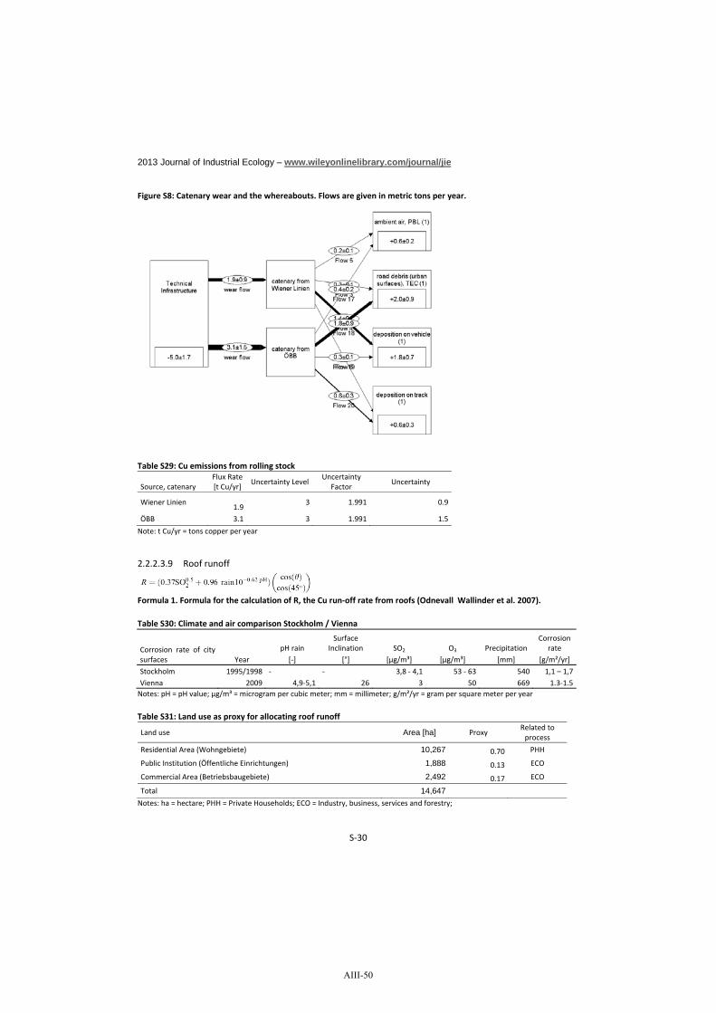
2013 Journal of Industrial Ecology – www.wileyonlinelibrary.com/journal/jie
S 30
Figure S8: Catenary wear and the whereabouts. Flows are given in metric tons per year.
Table S29: Cu emissions from rolling stock
Source, catenaryFlux Rate[t Cu/yr]
Uncertainty LevelUncertainty
FactorUncertainty
Wiener Linien1.9
3 1.991 0.9
ÖBB 3.1 3 1.991 1.5
Note: t Cu/yr = tons copper per year
2.2.2.3.9 Roof runoff
Formula 1. Formula for the calculation of R, the Cu run off rate from roofs (Odnevall Wallinder et al. 2007).
Table S30: Climate and air comparison Stockholm / Vienna
Corrosion rate of citysurfaces Year
pH rainSurface
Inclination SO2 O3 PrecipitationCorrosion
rate[ ] [°] [μg/m³] [μg/m³] [mm] [g/m²/yr]
Stockholm 1995/1998 3,8 4,1 53 63 540 1,1 – 1,7Vienna 2009 4,9 5,1 26 3 50 669 1.3 1.5Notes: pH = pH value; μg/m³ = microgram per cubic meter; mm = millimeter; g/m²/yr = gram per square meter per year
Table S31: Land use as proxy for allocating roof runoff
Land use Area [ha] ProxyRelated toprocess
Residential Area (Wohngebiete) 10,267 0.70 PHH
Public Institution (Öffentliche Einrichtungen) 1,888 0.13 ECO
Commercial Area (Betriebsbaugebiete) 2,492 0.17 ECO
Total 14,647Notes: ha = hectare; PHH = Private Households; ECO = Industry, business, services and forestry;
AIII-50

2013 Journal of Industrial Ecology – www.wileyonlinelibrary.com/journal/jie
S 31
2.2.2.3.10 Waste water flows
Table S32: Transfer Coefficients for Cu in WWTP
Material flow
TransferCoefficients Flux Rate
[%] [t Cu/yr]
Grill Material 6.0 1.0
Sewage Sludge 84.2 13.6
Effluents 9.8 1.6
Total 100 16.2Notes: t Cu/yr = metric tons copper per year
Table S33: Cu in waste water coming from anthropogenic activities in PHH
Source Flux Rate Reference
[mg/cap/yr]
Cu from food preparation 70 (Baccini et al. 1993)
Cu from washing dishes 25 (Baccini et al. 1993)
Cu in toilet paper (from recycling paper) 64 (Baccini et al. 1993)
Cu from product use 30 (I C Consultants Ltd 2001)
Cu from washing clothes 218 (Baccini et al. 1993)
Cu from cleaning living areas 436 (Baccini et al. 1993)
Total 843
Note: mg/cap/yr = milligram per capita per year
Table S34: Cu in waste water coming from humans
Source Flux Rate Reference
[mg/cap/yr]
Cu in feces 708 (I C Consultants Ltd 2001)
Cu in urin 5 (Lampert et al. 1997)
Cu in skin particles 47 (Lampert et al. 1997)
Cu in human off flows 760
Notes: mg/cap/yr = milligram per capita per year
AIII-51
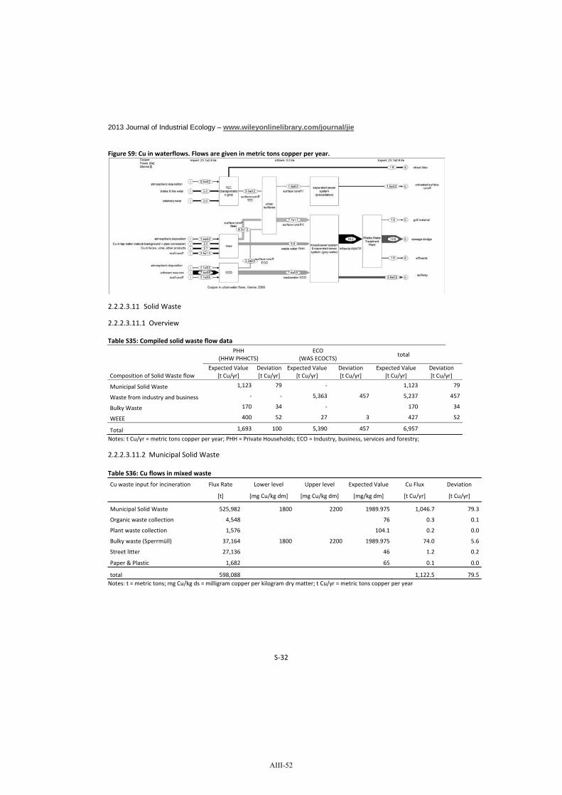
2013 Journal of Industrial Ecology – www.wileyonlinelibrary.com/journal/jie
S 32
Figure S9: Cu in waterflows. Flows are given in metric tons copper per year.
2.2.2.3.11 Solid Waste
2.2.2.3.11.1 Overview
Table S35: Compiled solid waste flow data
Composition of Solid Waste flow
PHH(HHW PHHCTS)
ECO(WAS ECOCTS)
total
Expected Value[t Cu/yr]
Deviation[t Cu/yr]
Expected Value[t Cu/yr]
Deviation[t Cu/yr]
Expected Value[t Cu/yr]
Deviation[t Cu/yr]
Municipal Solid Waste 1,123 79 1,123 79
Waste from industry and business 5,363 457 5,237 457
Bulky Waste 170 34 170 34
WEEE 400 52 27 3 427 52
Total 1,693 100 5,390 457 6,957
Notes: t Cu/yr = metric tons copper per year; PHH = Private Households; ECO = Industry, business, services and forestry;
2.2.2.3.11.2 Municipal Solid Waste
Table S36: Cu flows in mixed waste
Cu waste input for incineration Flux Rate Lower level Upper level Expected Value Cu Flux Deviation
[t] [mg Cu/kg dm] [mg Cu/kg dm] [mg/kg dm] [t Cu/yr] [t Cu/yr]
Municipal Solid Waste 525,982 1800 2200 1989.975 1,046.7 79.3
Organic waste collection 4,548 76 0.3 0.1
Plant waste collection 1,576 104.1 0.2 0.0
Bulky waste (Sperrmüll) 37,164 1800 2200 1989.975 74.0 5.6
Street litter 27,136 46 1.2 0.2
Paper & Plastic 1,682 65 0.1 0.0
total 598,088 1,122.5 79.5Notes: t = metric tons; mg Cu/kg ds = milligram copper per kilogram dry matter; t Cu/yr = metric tons copper per year
AIII-52

2013 Journal of Industrial Ecology – www.wileyonlinelibrary.com/journal/jie
S 33
Table S37: Cu concentrations is various mixed waste fractionsCu
content
Cu content in waste [mg/kg] Reference
Municipal solid waste 2000 (Skutan and Rechberger 2007, p. 82; Skutan and Brunner 2006, p. 236)
Average Organic Waste Collection (Biotonne) 76 (Umweltbundesamt 2000)
Average Plant Waste Collection (Grünschnitt) 104 (Umweltbundesamt 2000)
Cu concentration in street litter 46 (Boller 2002)
Cu concentration in bulky waste 2.000 (Hausmann 2005)
Cu concentration in paper and plastic 65 (Arx 2006)Note: mg/kg = milligram per kilogram
2.2.2.3.11.3 Waste from industry and businessTable S38: Waste from industry and business
key N°
Waste from industry and business
Amount of Wastein Vienna Cu Content Cu in waste flow
Note
[t/yr] [%]
ExpectedValue
[t Cu/yr]
Deviation[t Cu/yr]
35301 Waste from punching, blanking (isrecycled)
8,831 12.5% 1,104 191
35315 Non ferrous metal scrap (isrecycled)
2,993 55% 1,646 285
51104 Electroplating sludge 142 15 12% 37 14
51530 Cu chloride 1,506 47 65% 832 86
35310 Cu scrap from production industry 1,839 90 99,9% 1,744 290 See sec. 2.2.2.3.3
Total 5,363 457
Notes: t/yr = metric tons per year; t Cu/yr = metric tons copper per year; key N° = key number according to the Austrian wastemanagement directive
2.2.2.3.11.4 Bulky waste
Table S39: Allocation of bulky waste flows
Flow
Collected bulky waste inVienna, from PHH and ECO
Cu concentrationLower range
Cu concentrationUpper range
Geometricmean
Cu Flux
[t/yr] [mg/kg] [mg/kg] [mg/kg] [t Cu/yr]
Bulky Waste 69,422 1800.00 3300.00 2437.212 169
Notes: t/yr = metric tons per year; mg/kg = milligram per kilogram; t Cu/yr = metric tons copper per year;
AIII-53

2013 Journal of Industrial Ecology – www.wileyonlinelibrary.com/journal/jie
S 34
2.2.2.3.12 WEEETable S40: WEEE from PHH
WEEE from PHH
Flow of goods,expected value
Cu concentrationLower range
Cu concentrationUpper range
Geometricmean
Cu Flux rate Deviation
[t] [%] [%] [%] [t Cu/yr] [t Cu / yr]
Large WEEE 2,983 3.90 8.00 5.586 167 37
Fridges & Freezers 2,103 1.00 4.00 2.000 42 21
Monitors 2,387 3.90 7.80 5.515 132 28
Small WEEE 1,572 2.90 5.00 3.808 60 10
SumWaste PHH WEEE 9,044 400 52
Notes: t/yr = metric tons per year; t Cu/yr = metric tons copper per year;
Table S41: WEEE from ECO
WEEE from ECO
Flow of goods,expected value
Cu concentrationLower range
Cu concentrationUpper range
Geometricmean
Cu Flux rate Deviation
[t] [%] [%] [%] [t Cu/yr] [t Cu / yr]
Small WEEE 198 3.90 8.00 5.586 11 2
Cu in WEEE Waste 139 1.00 4.00 2.000 3 1
Large WEEE 158 3.90 7.80 5.515 9 2
Fridges & Freezers 104 2.90 5.00 3.808 4 1
SumWaste PHH WEEE 599 27 3Notes: t = metric tons; t Cu/yr = metric tons copper per year;
Table S42: Allocation of WEEE flows
Description value unit
Collected from private households 61,390,135 t/yr
Collected from economy 4,067,869 t/yr
Ratio = Proxy ECO/PHH 0,07Note: t/yr = metric tons per year; PHH = Private Households; ECO = Industry, business, services and forestry;
2.2.2.3.13 Exported products (PRO ANTEXA)
Table S43: Compiled data for exported flowsFlow Name Flux rate Deviation Calculation procedure and references
Flow acronym [t Cu/yr] [t Cu/yr]
VEH VEHECO Exported vehicles 138 68 See flow “Exported Vehicles”, sec. 2.2.2.3.4
Products fromproducing industry
950 After data are not available, we assumed that 50% of thedifference from imported Cu for producing industries (seeflow PRO EXAECO) and the waste from production (see flowWAS ECOCTS). 0.5*(4,600 2,700)=950
PRO ANTEXA 1,088
Note: t Cu/yr = metric tons copper per year;
2.2.2.3.14 Exported waste including recyclables (REC CTSECO)To estimate the recycling flow, we used the recycling potential of six generated waste flows, combined themwith individual information regarding the whereabouts in recycling facilities.
AIII-54

2013 Journal of Industrial Ecology – www.wileyonlinelibrary.com/journal/jie
S 35
Table S44: Cu waste including potential recyclables
Potential recyclables in waste flow Calculation procedure and references
Recyclables and wasteExpected Value
[t Cu/yr]Deviation[t Cu/yr]
Demolition Material (construction waste,concrete demolition, Construction anddemolition timber)
835PHH (522)ECO (223)TEC (90)
135(123)(53)(14)
See flow “Construction material”, sec. 2.2.2.3.2.835 t Cu/yr is estimated for demolition material.Even 75% (Ableidinger et al. 2007) of demolitionmaterial was sent out of the city, we assumed that100% of Cu is sent out to recycling facilities out ofVienna.
Cu scrap 3,235PHH (2,092)ECO (894)TEC (249)
532(486)(207)(62)
See flow “Construction material”, sec. 2.2.2.3.2.Cu scrap was reported in the Viennese wastestatistics with an amount of 5,254 t/yr. An averageCu content of 90 99.5% results 4,982 t Cu/yr ofwhich 3,235 are related to construction waste thatgoes to recycling facilities out of Vienna.
Cables 870PHH (369ECO (158)TEC (343)
127(86)(37)(86)
See flow “Construction material” sec. 2.2.2.3.2.The Viennese waste statistics accounted 2,400 tcables [42]; measurements reveal a Cu content of37% in cables within demolition material [47].Combining the two factors results 870 t Cu/a.
Subtotal, construction waste 4,940 563
Waste from industry and business 5,363 457 See flow “solid waste”, sec. 2.2.2.3.11
Bulky Waste 170 34 See flow “solid waste”, sec. 2.2.2.3.11
WEEE 427 52 See flow “solid waste”, sec. 2.2.2.3.11WEEE is collected and partly dismantled in Viennabut separation to the metal fractions occurs invarious specialized treatment plants outside the city(Spitzbart 2012). The total amount of Cu in WEEEcollected in Vienna is ~430 t/yr.
Recycled End of Live Vehicles 235 39 See flow “EOL vehicles”, sec. 2.2.2.3.4
Total 11,135 729
Note: t Cu/yr = metric tons copper per year
2.2.2.3.15 HarvestPlant uptake of Cu from soil range are estimated to be 43 g/(ha*a) in farmland to 51 g/(ha*a)in grassland(Zethner et al. 2007; Kühnen and Goldbach 2004) . If the plants are further harvested, this amount of Cu isactively removed from the soil. With an agricultural area of ~ 6.000 ha, the Cu flow in harvest is estimated tobe ~ 0,3 t/yr. To test this values probability, detailed harvest information (Fitzthum 2009) combined with Cutake up values for Crops, Wine and Fruit production which was published in an Austrian study (Berger et al.2011). The Sum of Cu take up in harvest is therefore estimated to be 0,3 t/yr (uncertainty factor: 1,34).
Table S45: Agricultural production
Cu in harvest products
Harvest 2008 Cu take up Cu
[ha] [kg Cu/ha/yr] [kg]
Agriculture & Horticulture 5,600 0,045 252
Wine production 600 0.01 6
Fruit production 70 0.03 2
Sum 6,270 ~ 260Notes: ha = hectare; kg Cu/ha/yr = kilogram copper per hectare per year; kg = kilogram;
AIII-55

2013 Journal of Industrial Ecology – www.wileyonlinelibrary.com/journal/jie
S 36
2.2.2.3.16 Pesticides
Table S46: Pesticide inputs on soil
Pesticide Input Area Pesticide rates Cu Flux rate
[ha] [kg Cu/ha/yr] [t/yr]
Viticulture organic 109 3.000 0.327
Fruit Production organic 12 3.000 0.036
Agriculture & Horticulture organic 1,009 1.400 1.413
Viticulture 497 1.000 0.497
Fruit Production 55 1.500 0.082
Agriculture & Horticulture 4,599 0.000 0.000
Total 6,281 2.356Notes: ha = hectare; kg Cu/ha/yr = kilogram copper per hectare per year; t = metric tons;
2.2.2.3.17 Fertilizer
Table S47: Fertilizer inputs on soil
Fertilizer Input Area Fertilizer rate Cu flux rate
[ha] [kg Cu/(ha/a)] [t/yr]
Viticulture organic 109 0.200 0.022
Fruit Production organic 12 0.200 0.002
Agriculture & Horticulture organic 1,009 0.550 0.555
Viticulture 497 0.030 0.015
Fruit Production 55 0.030 0.002
Agriculture & Horticulture 4,599 0.350 1.609
Total 6,281 2.205Notes: ha = hectare; kg Cu/ha/yr = kilogram copper per hectare per year; t/yr = metric tons per year;
2.2.2.3.18 Cu stock in technical infrastructure (TECstock)
Table S48: Cu stocks in electricity grid
Electricity gridLength of network
[km]Cu content in
[t/km]Amount of Cu [t]
min max min max
Highest voltage 54 10.72 583 583
High voltage 375 10.72 4,015 4,015
Medium voltage 6,844 5.09 34,837 34,837
Low voltage 11,255 4.07 45,809 45,809
Overhead power lines 3,747 0.75 1.34 2,807 5,012
Sum 22,276 88,052 90,257
89,154Notes: km = kilometer; t/km = metric tons per kilometer; min = minimum value; max = maximum value
AIII-56
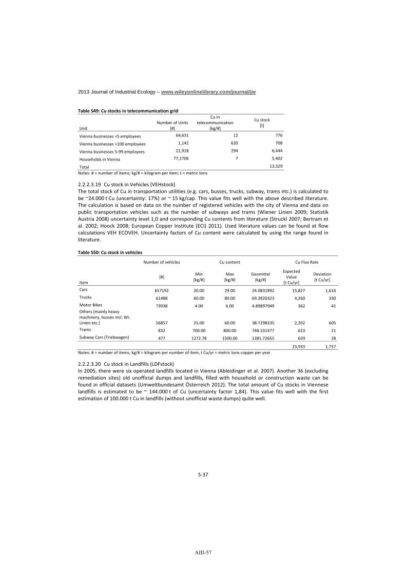
2013 Journal of Industrial Ecology – www.wileyonlinelibrary.com/journal/jie
S 37
Table S49: Cu stocks in telecommunication grid
UnitNumber of Units
[#]
Cu intelecommunication
[kg/#]
Cu stock[t]
Vienna businesses <5 employees 64,631 12 776
Vienna businesses >100 employees 1,142 620 708
Vienna businesses 5 99 employees 21,918 294 6,444
Households in Vienna 77,1706 7 5,402
Total 13,329
Notes: # = number of items; kg/# = kilogram per item; t = metric tons
2.2.2.3.19 Cu stock in Vehicles (VEHstock)The total stock of Cu in transportation utilities (e.g. cars, busses, trucks, subway, trams etc.) is calculated tobe ~24.000 t Cu (uncertainty: 17%) or ~ 15 kg/cap. This value fits well with the above described literature.The calculation is based on data on the number of registered vehicles with the city of Vienna and data onpublic transportation vehicles such as the number of subways and trams (Wiener Linien 2009; StatistikAustria 2008) uncertainty level 1,0 and corresponding Cu contents from literature (Struckl 2007; Bertram etal. 2002; Hoock 2008; European Copper Institute (ECI) 2011). Used literature values can be found at flowcalculations VEH ECOVEH. Uncertainty factors of Cu content were calculated by using the range found inliterature.
Table S50: Cu stock in vehicles
Number of vehicles Cu content Cu Flux Rate
Item[#]
Min[kg/#]
Max[kg/#]
Geomittel[kg/#]
ExpectedValue
[t Cu/yr]
Deviation[t Cu/yr]
Cars 657192 20.00 29.00 24.0831892 15,827 1,616
Trucks 61488 60.00 80.00 69.2820323 4,260 330
Motor Bikes 73938 4.00 6.00 4.89897949 362 41Others (mainly heavymachinery, busses incl. Wr.Linien etc.) 56857 25.00 60.00 38.7298335 2,202 605
Trams 832 700.00 800.00 748.331477 623 21
Subway Cars (Triebwagen) 477 1272.78 1500.00 1381.72655 659 28
23,933 1,757Notes: # = number of items, kg/# = kilogram per number of item; t Cu/yr = metric tons copper per year
2.2.2.3.20 Cu stock in Landfills (LDFstock)In 2005, there were six operated landfills located in Vienna (Ableidinger et al. 2007). Another 36 (excludingremediation sites) old unofficial dumps and landfills, filled with household or construction waste can befound in official datasets (Umweltbundesamt Österreich 2012). The total amount of Cu stocks in Vienneselandfills is estimated to be ~ 144.000 t of Cu (uncertainty factor 1,84). This value fits well with the firstestimation of 100.000 t Cu in landfills (without unofficial waste dumps) quite well.
AIII-57

2013 Journal of Industrial Ecology – www.wileyonlinelibrary.com/journal/jie
S 38
Table S51: Cu stock in landfills
Amount of Cu Uncertaintyfactor[t] Min [t] Max
Excavated Soil (1)+(2)+(3)+(4) 6,845,900 200 400 1,49Construction Waste (5) 11,300,000 900 8.000 2,90Treated municipal solid waste 27.000 71.000 1,62Slag concrete as construction material (6)+(7)+(8) 27,240,000 30.000 35.000 3,24Waste dumps (unofficial) 35,690,400 24.000 93.000 2,02Total sum of Cu stock in landfills 82.000 210.000 1,84Mean Value 144.000 1,84Notes: t = metric tons
Table S52: Landfills in ViennaLandfill Landfill Type Approved
volumeAvailablecapacity
Depositedwastevolume
Density*) Mass N°
[m3] [m3] [m3] [t/m3] [t]Deponie Max Excavated soil 97.000 0 97.000 1,7 164.900 (1)Nassbaggerung Transportbeton Excavated soil 2.900.000 300.000 2.600.000 1,7 4.420.000 (2)
Nassbaggerung Readymix Excavated soil 1.600.000 350.000 1.250.000 1,7 2.125.000 (3)
Deponie Rendezvousberg (Kleedorfer) Excavated soil 250.000 170.000 80.000 1,7 136.000 (4)Deponie Langes Feld (3 Kompartimente) Construction w.
Mass wasteMunicipal solid w.
7.400.0002.000.0001.600.000
1.750.0001.650.0001.500.000
5.650.000350.000100.000
22,42,8
11.300.000840.000280.000
(5)(6)(7)
Deponie Rautenweg Mass waste 14.000.000 3.000.000 11.000.000 2,4 26.400.000 (8)
total 29.847.000 8.720.000 21.127.000 45.665.900
Note: * = own estimation; m3 = cubic meter; t/m3 = metric tons per cubic meter; t = metric tons
Deposited wastes include excavated soil (usually from construction sites), construction waste and treatedmunicipal waste according to Austrian landfill regulations and furthermore some municipal solid waste isstored temporarily. Using Cu concentrations from earlier calculations for excavated soil (28–61 mg/kg),construction waste (80 670 mg/kg) and municipal solid waste (1000 2600 mg/kg) the total Cu stock wascalculated. Especially for the landfills “Langes Feld” and “Rautenweg” calculations are difficult. Due to theirage, it is difficult to determine a Cu content of the former input. For example, “Langes Feld” was originallybuilt to receive construction and demolition waste from World War II. Additionally to the type of landfill,slags which are used as building material in Viennese landfills and their input since 1964 (when the firstMSW incineration plan in Vienna was established) were estimated. Here, the input of 2008, calculated with~ 1.100 t/yr as well as capacities of incineration plants since 1964 were used as a base value.Additionally to official landfills, waste dumps or suspected waste dumps with a total Volume of ~ 30 Mio m³were included into calculations (Umweltbundesamt Österreich 2012). With an average density of 1,0–1,2t/m³ (Fellner 2012) and contents (partly suspected, partly tested) as a mixture of untreated municipal solidwaste and construction waste (with unknown percentages), Cu stocks are estimated to be between 24.000and 90.000 t.
AIII-58

2013 Journal of Industrial Ecology – www.wileyonlinelibrary.com/journal/jie
S 39
2.2.2.3.21 Cu stock in urban soil (UPVstock)Figure S10: Substance concentration in parks with playgrounds, given in milligram per kilogram (mg/kg). The box isdefined by the 10% and 90% percentile and the median. The red and blue bars indicate orientation values.
Table S53: Median concentrations in parks with playgrounds given in milligram per kilogram (mg/kg)As Cd Co Cr Cu Hg Mo Ni Pb V Zn B(a)P PAK6 PAK16
median 8,1 0,5 7,9 37,5 46,0 0,5 0,9 27,0 75,0 34,0 158,0 0,2 0,9 1,8Eikman & Klokeplaygrounds, BW2 20 2 30 50 50 0,5 5 40 200 50 300 1
0.01
0.1
1
10
100
1000
As Cd Co Cr Cu Hg Mo Ni Pb V Zn B(a)P PAK6 PAK16
subs
tanc
e co
ncen
tratio
n [m
g/kg
]
Min Outlier Max OutlierEikman & Kloke (multifunctional use BW I) Eikman & Kloke (playgrounds BW II)
AIII-59
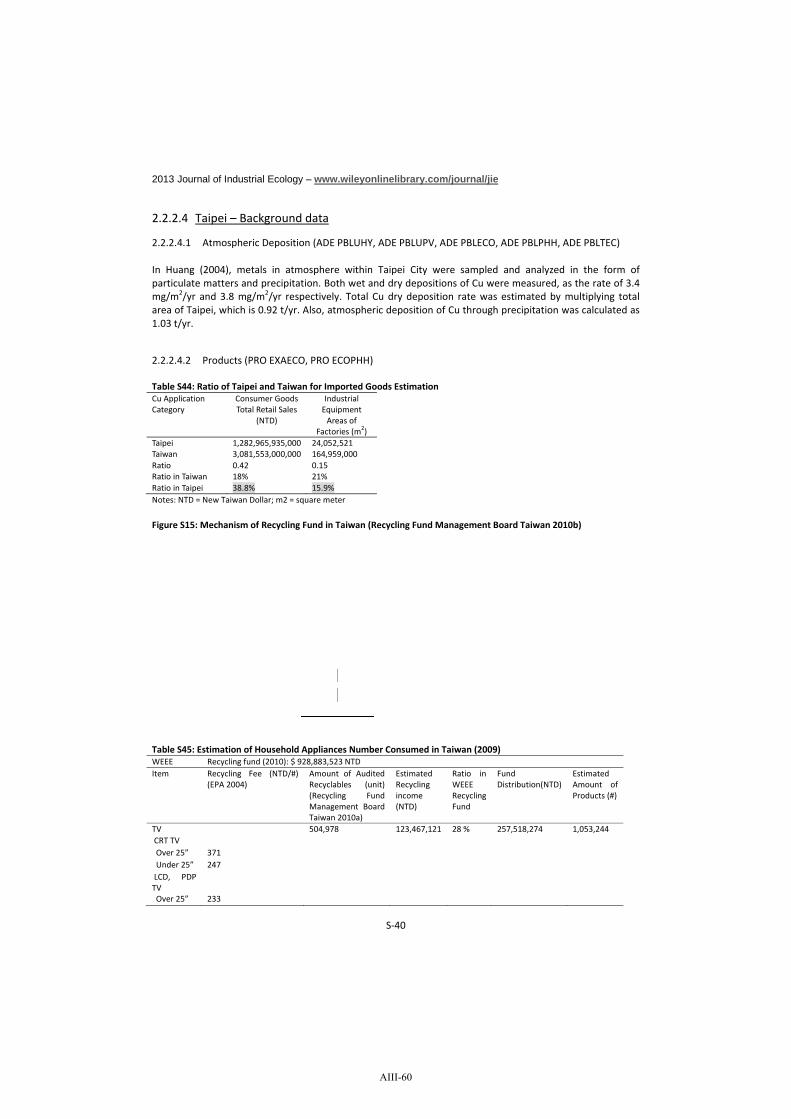
2013 Journal of Industrial Ecology – www.wileyonlinelibrary.com/journal/jie
S 40
2.2.2.4 Taipei – Background data
2.2.2.4.1 Atmospheric Deposition (ADE PBLUHY, ADE PBLUPV, ADE PBLECO, ADE PBLPHH, ADE PBLTEC)
In Huang (2004), metals in atmosphere within Taipei City were sampled and analyzed in the form ofparticulate matters and precipitation. Both wet and dry depositions of Cu were measured, as the rate of 3.4mg/m2/yr and 3.8 mg/m2/yr respectively. Total Cu dry deposition rate was estimated by multiplying totalarea of Taipei, which is 0.92 t/yr. Also, atmospheric deposition of Cu through precipitation was calculated as1.03 t/yr.
2.2.2.4.2 Products (PRO EXAECO, PRO ECOPHH)
Table S44: Ratio of Taipei and Taiwan for Imported Goods EstimationCu ApplicationCategory
Consumer GoodsTotal Retail Sales
(NTD)
IndustrialEquipmentAreas of
Factories (m2)Taipei 1,282,965,935,000 24,052,521Taiwan 3,081,553,000,000 164,959,000Ratio 0.42 0.15Ratio in Taiwan 18% 21%Ratio in Taipei 38.8% 15.9%Notes: NTD = New Taiwan Dollar; m2 = square meter
Figure S15: Mechanism of Recycling Fund in Taiwan (Recycling Fund Management Board Taiwan 2010b)
Table S45: Estimation of Household Appliances Number Consumed in Taiwan (2009)WEEE Recycling fund (2010): $ 928,883,523 NTDItem Recycling Fee (NTD/#)
(EPA 2004)Amount of AuditedRecyclables (unit)(Recycling FundManagement BoardTaiwan 2010a)
EstimatedRecyclingincome(NTD)
Ratio inWEEERecyclingFund
FundDistribution(NTD)
EstimatedAmount ofProducts (#)
TV 504,978 123,467,121 28 % 257,518,274 1,053,244CRT TVOver 25” 371Under 25” 247LCD, PDPTVOver 25” 233
AIII-60
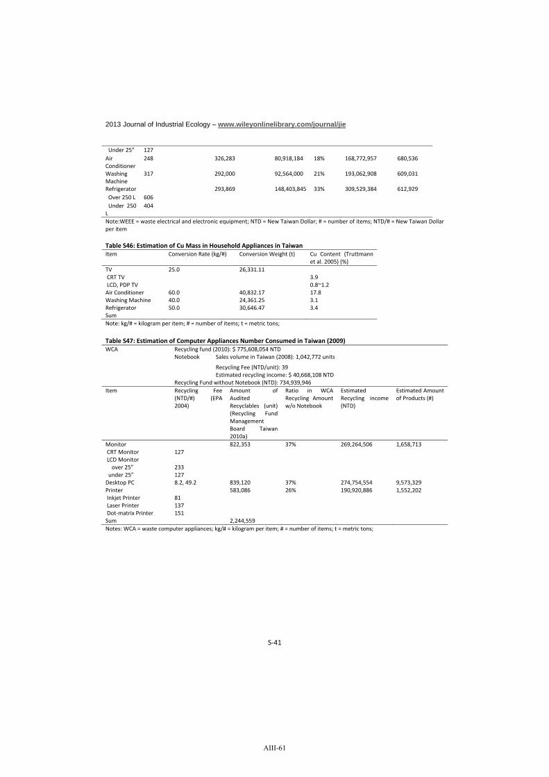
2013 Journal of Industrial Ecology – www.wileyonlinelibrary.com/journal/jie
S 41
Under 25” 127AirConditioner
248 326,283 80,918,184 18% 168,772,957 680,536
WashingMachine
317 292,000 92,564,000 21% 193,062,908 609,031
Refrigerator 293,869 148,403,845 33% 309,529,384 612,929Over 250 L 606Under 250L
404
Note:WEEE = waste electrical and electronic equipment; NTD = New Taiwan Dollar; # = number of items; NTD/# = New Taiwan Dollarper item
Table S46: Estimation of Cu Mass in Household Appliances in TaiwanItem Conversion Rate (kg/#) Conversion Weight (t) Cu Content (Truttmann
et al. 2005) (%)TV 25.0 26,331.11CRT TV 3.9LCD, PDP TV 0.8~1.2Air Conditioner 60.0 40,832.17 17.8Washing Machine 40.0 24,361.25 3.1Refrigerator 50.0 30,646.47 3.4SumNote: kg/# = kilogram per item; # = number of items; t = metric tons;
Table S47: Estimation of Computer Appliances Number Consumed in Taiwan (2009)WCA Recycling fund (2010): $ 775,608,054 NTD
Notebook Sales volume in Taiwan (2008): 1,042,772 units
Recycling Fee (NTD/unit): 39Estimated recycling income: $ 40,668,108 NTD
Recycling Fund without Notebook (NTD): 734,939,946Item Recycling Fee
(NTD/#) (EPA2004)
Amount ofAuditedRecyclables (unit)(Recycling FundManagementBoard Taiwan2010a)
Ratio in WCARecycling Amountw/o Notebook
EstimatedRecycling income(NTD)
Estimated Amountof Products (#)
Monitor 822,353 37% 269,264,506 1,658,713CRT Monitor 127LCD Monitorover 25” 233
under 25” 127Desktop PC 8.2, 49.2 839,120 37% 274,754,554 9,573,329Printer 583,086 26% 190,920,886 1,552,202Inkjet Printer 81Laser Printer 137Dot matrix Printer 151Sum 2,244,559Notes: WCA = waste computer appliances; kg/# = kilogram per item; # = number of items; t = metric tons;
AIII-61

2013 Journal of Industrial Ecology – www.wileyonlinelibrary.com/journal/jie
S 42
Table S48: Estimation of Cu in Computer Appliances in TaiwanItem Conversion Rate
(kg/#)Conversion Weight (t) Cu Content (%)
Notebook 4.0 4,171.09 1.00% (Oguchi et al.2011)
Monitor 12.0 19,904.56 7.83% (Truttmann etal. 2005)
Desktop PC 12.0 114,879.95 0.90%a
Printer 8.5 13,193.72 3.20%a
SumNotes: kg/# = kilogram per item; t = metric tons;
2.2.2.4.3 Construction Material (CON EXAECO, CON ECOTEC, CONECOPHH, CWA ECOCTS, CWA TECCTS,CWA PHHCTS)
Table S49: Estimation of Cu in Construction WasteTaipei Value UnitTotal demolished floor area 25,000 m2
Waste from C&D waste (Huang 1998) 1~1.28 tCu content in C&D waste (Huang 1998) 670~2,587 mg/kgNotes: m2 = square meter; t = metric tons; mg/kg = milligram per kilogram
Table S50: Results of Cu in Construction Waste from PHH, CTS, and ECOLand Use in Taipei Area (ha) ProportionUrbanized Area 12,993.11 100%PHH 41%Residential District 3,793.06Commercial District 866.36Administration District 80.97Cultural District 73Special District 190Others 260.45ECO 3%Industrial District 419.49TEC 56%Public Facilities 7,309.78Notes: ha = hectare
2.2.2.4.4 Vehicles (VEH ECOVEH, WAS VEHCTS, VEH UID, VEH VEHECO)
Table S51: Estimation of Sales Volume of Vehicles in Taipei 2009NewlyRegisteredNumber
SalesVolume
Average weightedweights per unit (kg)(Liu 2009)
Mass of SalesVolume (t/yr)
TaiwanCars 6,769,845 294,423Scooters/Motorcycles 14,604,330 478,268TaipeiCars 721,326 31,371 1,034 32,437,332.57Scooters/Motorcycles 1,092,788 35,787 90.85 3,251,251.27Sum 35,688,583.84
Notes: kg = kilogram; t/yr = metric tons per year
AIII-62

2013 Journal of Industrial Ecology – www.wileyonlinelibrary.com/journal/jie
S 43
Table S52: Estimation of Recycled Vehicles in TaipeiNewlyRegisteredNumber [#]
Average weighted weightsper unit (kg)(Liu 2009)
Recycled Mass(t)
TaiwanCars 6,769,845 1,034 130,791Scooters/Motorcycles 14,604,330 90.85 21,994TaipeiCars 721,326 1,034 195Scooters/Motorcycles 1,092,788 90.85 23Sum
Notes: t = metric tons; # = number of items Table S53: Estimation of Exported Vehicles
Newly Registered Number [#] Change of Registration (2009 2008)TaiwanCars 6,769,845 42,929Scooters/Motorcycles 14,604,330 238,888TaipeiCars 721,326 4,574Scooters/Motorcycles 1,092,788 17,875Sum
Note: # = Number of items
2.2.2.4.5 Solid waste (HWW PHHCTS, WAS ECOCTS)
Table S54: Result of Cu Mass in Household WasteSource of Waste Cu Content Amount (t/yr)By Cleaning Squads
184.92~577.13 mg/kg368,253.67
By People Themselves 13,974.27Recyclables (%)TV 0.8~3.9 5,302.27Air Conditioner 17.8 8,222.33Washing Machine 3.1 4,906Refrigerator 3.4 6,171.25Laptop 1 75.29Monitor 7.83 4,144.66Motherboard 0.9 4,229.16Printer 3.2 2,081.62
SumNote: t/yr = metric tons per year
2.2.2.4.6 Incineration: Mixed waste, exported residues for underground storage, residues Disposablewaste (WAS CTSINC, TTR INCEXA, RES INCLDF)
Table S55: Residues of IncineratorsAmount (t) Cu Content (mg/kg) (Chen
2008)Fly Ash 20,000 1028~1220Bottom Ash 110,000 889~3136Note: t = metric ton; mg/kg = milligram per kilogram
AIII-63

2013 Journal of Industrial Ecology – www.wileyonlinelibrary.com/journal/jie
S 44
2.2.2.4.7 Composting: Compostable waste, residues, compost as fertilizer (WAS CTSCOM, RES COMCTS,COM COMUPV)
Table S56: Estimation of Compost Generated in Taipei CityData source Uncooked food waste (t/yr) Compost (t/yr) Cu content (mg/kg)Muzha Incinerator 16,625.3 221.15 0.69Waste in Taipei City 59,371.23 (Department of
Environmental Protection ofTaipei City Government2009)
789.76 0.69
Note: t/yr = metric tons per year; mg/kg = milligram per kilogram
2.2.2.4.8 Stocks in ECO, PHH
Table S57: Estimation of the In Use Household AppliancesItem Average Number
Per HundredHouseholds inTaipei (#)
EstimatedAmount of In useStock (#)
Conversion Rate(kg/#)
ConversionWeight(t)
Cu Content (%)(Oguchi et al.2011)
TV 155.87 1,500,764.68 25.0 37,519.12 0.8~3.9Air Conditioner 224.39 2,160,496.48 60.0 129,629.79 17.8WashingMachine
99.26 955,706.05 40.0 38,228.24 3.1
Laptop 123.03 (IDCTaiwan 2008)
1,184,570.98 4.0 4,738.28 1.0
Desktop 123.03 1,184,570.98 12.0 14,214.85 0.9Note: # = number of items; kg/# = kilogram per item; t = metric ton;
Table S58: Information of the Tainan Case (construction completed in 1997)Structure Floors UsageAboveground 13 1F Shop
2F~13F Congregate HousingUnderground 3 B1~B3 Parking Lot
Table S59: Estimation of Wire and Cable Usage in BuildingsThe Tainan Case Amount Unit
Wire and Cable Used 17,763.84 kg
Total Floor Area 1.79 kg/m2
Total Floor Area in Taipei 171,185,000 m2
Estimated Wire and Cable Used 306,372,155 kg
Cu Content 40~60 (Ruhrberg 2006; Spatari et al. 2002) %
Note: kg = kilogram; kg/m2 = kilogram per square meter;
2.2.2.4.9 Stocks in VEH
AIII-64

2013 Journal of Industrial Ecology – www.wileyonlinelibrary.com/journal/jie
S 45
Table S60: Estimation of Cu Stock in TransportationVehicles Number of Registration/In
Operation (EnvironmentalProtection AdministrationExecutive Yuan 2010)
Average WeightedWeight Per Unit (kg) (Liu2009)
Cu Content
Cars 721,326 1,034 1.4%Scooters 1,092,788 90.85 1.4%Buses 2,628 60~80 kg/#
AIII-65

2013 Journal of Industrial Ecology – www.wileyonlinelibrary.com/journal/jie
S 46
2.3 Stock and flow resultsTable S54 shows the model inputs for each city in column (3), (4), (7), (8) and the balanced results in column(5), (6), (9), (10).
Table S54: Flow list.TAIPEI VIENNA
Flow Flow nameMass flow[t/yr]
± Massflow [t/yr]
Mass flow(calculated)
[t/yr]
± Mass flow(calculated)
[t/yr]Mass flow[t/yr]
± Massflow[t/yr]
Mass flow(calculated) [t/yr]
± Massflow
(calculated) [t/yr]
(1) (2) (3) (4) (5) (6) (7) (8) (9) (10)
ADE PBLECO Atmospheric Deposition ECO 0.02 0.00 0.02 0.00 1.10 0.19 1.09 0.19
ADE PBLPHH Atmospheric Deposition PHH 0.19 0.01 0.19 0.01 1.50 0.26 1.49 0.26
ADE PBLTEC Atmospheric Deposition TEC 0.28 0.02 0.28 0.02 0.90 0.15 0.90 0.15
ADE PBLUHY Atmospheric Deposition UHY 0.07 0.01 0.07 0.00 0.30 0.10 0.30 0.10
ADE PBLUPV Atmospheric deposition PV 0.29 0.02 0.29 0.02 2.80 0.50 2.76 0.49
COM ANTUPV Compost 0.04 0.01 0.04 0.00 1.40 0.30 1.40 0.21
CON ECOPHH Construction Material 8,164.59 1,420.10 8,164.59 1,420.10 6,567.00 838.00 6,567.00 838.00
CON ECOTEC Construction material 4,224.21 734.73 4224.21 734.73 2,448.00 376.00 2,448.00 376.00
CON EXAECOImported constructionmaterial
13,073.32 2,273.89 13,073.32 2,273.8911,817.00 1,390.00 11,817.00 1,390.00
CWA ECOCTS Construction waste ECO 2.79 1.36 2.82 1.36 1,275.00 217.00 1,266.04 212.19
CWA PHHCTS Construction waste PHH 150.86 73.44 223.07 69.99 2,983.00 509.00 2,933.70 443.42
CWA TECCTS Construction waste TEC 48.66 23.64 56.15 23.53 862.00 107.00 859.82 106.43
EFF WWSHYD Effluents 2.85 0.22 2.73 0.22 1.60 0.10 1.60 0.10
FER ECOUPV Fertilizer 0.00 0.00 2.20 0.30 2.20 0.30
HAR UPVECO Harvest 0.00 0.00 0.30 0.10 0.30 0.10
HHW PHHCTS Household waste 1,672.34 54.77 1,712.52 53.36 1,693.00 100.00 1,691.10 99.53
PAE TECPBL Particulate emissions 0.00 0.00 0.60 0.20 0.61 0.20
PAE VEHPBL Particulate emissions 6.10 2.67 0.84 0.03 5.00 2.50 5.94 0.63
PAE VEHTEC Particulate emissions 0.00 0.00 2.20 1.20 2.20 1.20
PES UANUPV Pesticides 0.00 0.00 2.40 0.30 2.40 0.30
PRO ECOEXA Exported Products 7,944.63 1,359.73 7,944.63 1,359.73 2,574.00 746.00 2,574.00 746.00
PRO ECOPHH Consumer goods & food 5,286.44 1,610.12 5,286.44 1,610.12 1,484.00 205.00 1,484.00 205.00
PRO EXAECO Imported products 15,773.73 2,743.58 15,773.73 2,743.58 8,827.00 728.00 8,827.00 728.00
RES INCLDF Residues 209.08 81.53 164.72 55.91 986.00 170.00 1,097.19 72.22
SPW WWSHYD Combined sewer overflow 0.00 0.00 3.80 0.80 3.86 0.78
SRO ECOWWS Surface runoff 0.02 0.01 0.02 0.01 2.20 0.50 2.18 0.49
SRO PHHWWS Surface runoff PHH 0.51 0.25 0.66 0.25 4.00 1.30 3.84 1.20
SRO TECWWS Surface runoff 0.35 0.18 0.43 0.18 3.30 1.50 3.09 1.35
SRO WMIHYD Surface Runoff 0.90 0.40 0.51 0.40 1.80 0.05 1.80 0.05
SSL WWSCTS sewage sludge 58.28 4.51 9.08 0.92 13.60 1.10 13.71 1.04
TTR INCEXAExported residues forunderground
0.00 0.0016.40 1.30 16.41 1.30
VEH ECOVEH vehicles 499.64 250.02 499.64 250.02 2,237.00 185.00 2,237.00 185.00
VEH UID Unidentified cars 0.00 0.00 498.00 330.00 498.00 330.00
VEH VEHECO EOL vehilces for export 88.95 44.42 88.95 44.42 138.00 68.00 138.00 68.00
AIII-66

2013 Journal of Industrial Ecology – www.wileyonlinelibrary.com/journal/jie
S 47
WAS CTSCOM Compostable waste 0.04 0.01 0.04 0.00 1.40 0.30 1.40 0.21
WAS CTSEXAExported waste incl.recyclables
2,738.32 184.80 2,281.03 119.6311,135.00 729.00 11,236.14 518.30
WAS CTSINC waste 209.08 81.26 164.72 55.91 1,137.00 80.00 1,113.59 72.21
WAS ECOCTS Solid waste ECO 58.42 22.64 65.28 22.54 5,390.00 457.00 5,350.26 410.20
WAS TECCTS street litter 0.00 0.00 1.80 0.05 1.80 0.05
WAS VEHCTS Waste vehicles 218.14 108.88 376.88 97.28 235.00 39.00 234.71 38.97WWAECOWWS
Wastewater ECO 0.00 0.007.40 1.90 7.07 1.59
WWAPHHWWS
Wastewater PHH 9.80 0.76 11.21 0.755.00 1.50 4.79 1.35
Note: t/yr = metric tons per year
Table S55: Stock listTaipei Vienna
Process Process name Mass [t] ± Mass [t] Mass [t] ± Mass [t]
EXA External Anthroposphere (input related)
EXAO External Anthroposphere (output related
LDF Landfill 144,000 61,000PHH Private Households 27,795 11,579 131,000 35,000DSR Dansuie/Danube River
TEC Transport / Energy / Communication Infrastructure 32,027 8,325 103,000 11,000UST Underground Storage
UHY Urban HydrosphereECO Urban Industry, Business, Services & Forestry / 215 27 40,000 14,000
UPV Urban Pedosphere & Vegetation 831 145 4,000 1,000VEH Vehicles 12,014 5,911 24,000 2,000Notes: t = metric tons
AIII-67

2013 Journal of Industrial Ecology – www.wileyonlinelibrary.com/journal/jie
S 48
Figure S11: Cu flow system of Vienna on 1st level: Snapshot for the year 2008. The stocks are given in gram per capita(g/cap) and the flows in gram per capita per year (g/cap/yr). The stock values as well as the alteration of stocks areshown in the boxes; the flows are represented as Sankey arrows proportional to the flux rate.
Figure S12: Cu flow system of Vienna on 2nd level: Snapshot for the year 2008. The stocks are given in gram per capita(g/cap) and the flows in gram per capita per year (g/cap/yr). The stock values as well as the alteration of stocks areshown in the boxes; the flows are represented as Sankey arrows proportional to the flux rate.
AIII-68

2013 Journal of Industrial Ecology – www.wileyonlinelibrary.com/journal/jie
S 49
Figure S13: Cu flow system of Taipei on 1st level: Snapshot for the year 2009. The stocks are given in gram per capita(g/cap) and the flows in gram per capita per year (g/cap/yr). The stock values as well as the alteration of stocks areshown in the boxes; the flows are represented as Sankey arrows proportional to the flux rate.
Figure S14: Cu flow system of Taipei on 2nd level: Snapshot for the year 2009. The stocks are given in gram per capita(g/cap) and the flows in gram per capita per year (g/cap/yr). The stock values as well as the alteration of stocks areshown in the boxes; the flows are represented as Sankey arrows proportional to the flux rate.
AIII-69

2013 Journal of Industrial Ecology – www.wileyonlinelibrary.com/journal/jie
S 50
3. References
Ableidinger, M., K. Arbter, W. Hauer, S. Sciri, and U. Volk. 2007. Wiener Abfallwirtschaftskonzept2007: Ist Zustand der Wiener Abfallwirtschaft. [Viennas Waste Managment Concept 2007:Status Quo.] Wien: Stadt Wien.
Arx, U. 2006. Kupfer: Verbrauch, Umwelteinträge und vorkommen. [Copper: Consumption,environmental impacts and availability.] Bern: Bundesamt für Umwelt.
Augustyn, R., P. Riess, and R. Bachl. 2010. Jahresbericht 2009 Luftgütemessungen derUmweltschutzabteilung der Stadt Wien gemäß Immissionsschutzgesetz Luft. [AnnualReport 2009 Air Quality Measurements according to Anti Pollution act conducted by thecity of Vienna.] Wien: Magistratsabteilung 22, Stadt Wien.
Baccini, P., H. Daxbeck, E. Glenck, and G. Henseler. 1993. Metapolis Güterumsatz undStoffwechselprozesse in den Privathaushalten einer Stadt. [Metabolis Material turnoverand metabolic processes in urban private households.] Zürich: Schweizerischer Nationalfondzur Förderung der Wissenschaft.
Bergbäck, B., K. Johansson, and U. Mohlander. 2001. Urban Metal Flows – A Case Study ofStockholm. Review and Conclusions.Water, Air, and Soil Pollution: Focus 1(3): 3 24.
Berger, E., G. Dersch, A. Dellantonio, K. Manner, B. Möbes Hansen, and M. Stemmer. 2011. Kupferals Pflanzenschutmittel Strategie für einen nachhaltigen und umweltschoneneden Einsatz.2. Zwischenbericht. [Copper as pesticide Strategies for sustainable and environmentalfriendly appliance.] 2. Zwischenbericht Wien: AGES Österreichische Agentur für Gesundheitund Ernährungssicherheit GmbH.
Bertram, M., T. E. Graedel, H. Rechberger, and S. Spatari. 2002. The contemporary European coppercycle: waste management subsystem. Ecological Economics 42(1 2): 43 57.
BMLFUW. 2011. Bundes Abfallwirtschaftsplan 2011. [Federal Waste Management Plan 2011.]Wien: Bundesministerium für Land u. Forstwirtschaft, Umwelt und Wasserwirtschaft.
Boller, M. 2002. Charakterisierung von Straßenabwasser Emissionen und Immissionen: VSAFortbildungskurs 2002 Straßenentwässerung der Zukunft.
Brunner, P. H. and D. M. Stampfli. 1993. Material Balance of a Construction Waste Sorting Plant.Waste Management & Research 11(1): 27 48.
Burkhardt, M., L. Rossi, N. Chevre, M. Boller, L. Steidle, J. Abrecht, F. Gächter, S. Knabl, and H.Kuppelwieser. 2005. Gewässerschutz bei Bahnanlagen Emittierte Stoffe imEisenbahnbetrieb der SBB und Grundlagen zu deren Umweltverhalten. [Water Protectionalong Railway Tracks Substance Release by Railway Operation of Swiss Federal Railways(SBB) and Fundamentals of their Environmental Behaviour.] Dübendorf, Schweiz: EAWAG.
Chen, Y. G. 2008. Statistical Model of Total Metal Concentration in Bottom Ash. Master Thesisthesis, National Taiwan University, Taipei, Taiwan.
Daxbeck, H., M. Stockinger, and B. Brand. 2006. Beitrag der Abfallwirtschaft zum KupferhaushaltÖsterreich. [Role of waste management in the Austrian copper metabolism.] Wien:Ressourcen Management Agentur.
Daxbeck, H., C. Lampert, L. S. Morf, R. Obernosterer, H. Rechberger, I. S. Reiner, and P. H. Brunner.1996. Der anthropogene Stoffhaushalt der Stadt Wien N, C und Pb. [The antropogenicmetabolism of Vienna Nitrogen, Carbon and Lead.] Wien: Technische Universität Wien.
Department of Environmental Protection of Taipei City Government. 2009. Statistics of WasteManagement in Taipei.
AIII-70

2013 Journal of Industrial Ecology – www.wileyonlinelibrary.com/journal/jie
S 51
www.dep.taipei.gov.tw/ct.asp?xItem=14974217&ctNode=39418&mp=110001. Accessed 12December 2012.
Department of Statistics. 2007. Estimation of Number of Vehicles Km Statistics in Taiwan. Taipei,Taiwan: Ministry of Transportation and Communication.
Dimitrova, D., J. Rauch, R. Gordon, and T. Graedel. 2007. Flow and Fates of Discarded Copper inSofia, Bulgaria, and New Haven CT, USA. Working Paper Number 12. Yale: Yale School ofForestry & Environmental Studies.
EAK. 2009. Tätigkeitsbericht 2008. [Annual Report 2008.] Wien: ElektroaltgeräteKoordinierungsstelle Austria GmbH (EAK).
Environmental Protection Administration Executive Yuan. 2010. Yearbook of EnvironmentalProtection Statistics, 2010.www.epa.gov.tw/ch/DocList.aspx?unit=24&clsone=501&clstwo=178&clsthree=168&busin=4177&path=9548. Accessed 12 December 2012.
EPA. 2004. Official Announcement of Fee Rates for Article and Container Recycling, Clearance, andDisposal (EPA Fei Tzu No. 0930097607C). Taipei, Taiwan: Executive Yuan EnvironmentalProtection Administration (EPA).
European Copper Institute (ECI). 2011. Transport. www.eurocopper.org/copper/coppertransport.html. Accessed 7 December 2011.
Fellner, J. 2012. Personal Communication with Fellner, J., Dichte von Altablagerungen. [Wastedensity in old landfills.].
Fenz, R. 1999. Gewässerschutz bei Entlastungsbauwerken der Mischkanalisation. [Water protectionof buildings regarding combined sewer systems.] Ph.D. thesis, Technische Universität Wien,Wien.
Figi, R., O. Nagel, M. Tuchschmid, P. Lienemann, U. Gfeller, and N. Bukowiecki. 2010. Quantitativeanalysis of heavy metals in automotive brake linings: A comparison between wet chemistrybased analysis and in situ screening with a handheld X ray fluorescence spectrometer.Analytica Chimica Acta 676(1 2): 46 52.
Fitzthum, R. 2009. Wiener Landwirtschaftsbericht 2008. [Annual agriculture report 2008.] Wien:Landwirtschaftskammer Wien.
Fricke, M. and H. U. Höhl. 2000. Schadstoffeintrag in Böden. In Müll und Abfall. München: ErichSchmidt Verlag.
Graedel, T. E., M. Bertram, K. Fuse, R. B. Gordon, R. Lifset, H. Rechberger, and S. Spatari. 2002. Thecontemporary European copper cycle: The characterization of technological copper cycles.Ecological Economics 42(1 2): 9 26.
Hauptverband der österreichischen Sozialversicherungsträger SV. 2011. Standardbeschäftigung inWien nach Wirtschaftsklassen seit 2008. Wien: Magistratsabteilung 05 Statistik.
Hausmann, M. 2005. Potential thermischer Verfahren zur stofflichen Abfallverwertung. [Potentialof thermal treatment for waste treatment.] Master thesis, Institut für Wassergüte,Ressourcenmanagement und Abfallwirtschaft, Technische Universität Wien, Wien.
Holzapfel, P. and R. Riedel. 2011. Personal Communication with Holzapfel, P. and R. Riedel,Verkehrsmodell Wien. [Traffic model Vienna.], 4 December 2011.
Hoock, R. 2008. Kupfer im Automobilbau. [Copper in car industry.] Metall 62. Jahrgang(10): 613617.
Huang, R. Y. 1998. The Status Quo and Investigation Framework of Pollution and Waste Generatedfrom Demolition. New Taipei City: Architecture and Building Research Institute, Ministry ofThe Interior.
AIII-71

2013 Journal of Industrial Ecology – www.wileyonlinelibrary.com/journal/jie
S 52
Hulskotte, J. H. J., M. Schaap, and A. Visschedijk. 2006. Brake wear from vehicles as an importantsource of diffuse copper pollution. 10th Int. Specialised Conference on Diffuse Pollution ansSustainable Basin Management, 18 22. September 2006, Instanbul. International WaterAssociation.
I C Consultants Ltd. 2001. Pollutants in Urban Waste Water and Sewage Sludge. Luxembourg:European Communities.
ICF. 2000. Wire in Automobiles: A one Million Tonne Market. Newsletter Issue 32 ICF InternationalCablemakers Federation.
ICF. 2001. Copper The Strategic Material (Newsletter Issue 35). ICF International CablemakersFederation.
IDC Taiwan. 2008. Sales Volume of PC in Taiwan 2008. www.idc.com.tw/about/archivenews.jsp.Accessed 11 December 2011.
Jien, S. H., C. C. Tsai, Z. Y. Hseu, and Z. S. Chen. 2011. Baseline Concentrations of Toxic Elements inMetropolitan Park Soils of Taiwan. Terrestrial and Aquatic Environmental Toxicology 5(1): 17.
Kalina, M., K. Leder, S. Kramer, and H. Puxbaum. 2000. Nasse Deposition im Land Wien Oktober 99September 00. [Wet deposition in Vienna, Oktober 99 September 00.] Vienna: TechnischeUniveristät Wien. Institut für Analytische Chemie. Abteilung für Umweltanalytik.
Keoleian, G., K. Kar, M. M. Manion, and J. W. Bulkley. 1997. Industrial Ecology of the Automobile: ALife Cycle Perspective. Warrendale: Society of Automotive Engineers, Inc.
Kreiner, P. 2004. Wiener Bodenbericht 2003: Untersuchung des Wiener Bodens auf Schwermetalleund polyaromatische Kohlenwasserstoffe. [Viennese soil report 2003: Investigation heavymetals and hydrocarbons in Viennese soils.] Wien: Stadt Wien.
Kroiss, H., L. S. Morf, C. Lampert, and M. Zessner. 2008. Optimiertes Stoffflussmonitoring für dieAbwasserentsorgung Wiens. [Optimized substance flow monitoring of the waste watertreatment plant in Vienna.] Wien: Technische Universität Wien.
Kronberger, R. 2011. Personal Communication with Kronberger, R., MVA Inputs 2008. Wien, 21November 2011.
Krook, J., A. Carlsson, M. Eklund, P. Frändegård, and N. Svensson. 2011. Urban mining: hibernatingcopper stocks in local power grids. Journal of Cleaner Production 19(9–10): 1052 1056.
Kubu, S. 2011. Personal Communication with Kubu, S., Roof surfaces and inclination of roofs inVienna. 6 December 2011.
Kühnen, V. and H. E. Goldbach. 2004. Schwermetallbilanzen verschiedener Betriebstypen:Eintragswege, Flüsse, Minderungspotential. [Heavy metal balances of different retailformats: Inputs, pathways, reduction potential.] www.usl.unibonn.de/pdf/Forschungsbericht%20118.pdf. Accessed 25 November 2011. Bonn:Ministerium für umwelt und Naturschutz, Landwirtschaft und Verbrauherschutz NordrheinWestfalen.
Lampert, C., W. Stark, R. Kernbeis, and P. H. Brunner. 1997. Stofffflussanalyse derSiedlungsentwässerung der beiden Regionen "Gresten" und "Grafenwörth". [Susbtance flowanalysis of regional water discharge.] Wien: Technische Universität Wien.
Lebhart, G. 2010. Statistisches Jahrbuch der Stadt Wien 2010. [Statistical Yearbook of Vienna 2010.]Vienna: Magistrat der Stadt Wien, Magistratsabteilung 5 Finanzwesen.
Lehmann, T. 2011. Personal Communication with Lehmann, T., Wastewater input into Viennaswaste water system, ratio of mixed/separated sewer system in Vienna. Vienna, 20 July 2011.
AIII-72

2013 Journal of Industrial Ecology – www.wileyonlinelibrary.com/journal/jie
S 53
Lin, J. U. 2003. A Study on the Operation Performance for the Transmission Line System of TaichungPower Supply Branch of Taiwan Power Company Master Thesis thesis, Taichung Healthcareand Management University, Taichung.
Liu, J. C. 2009. The Project of Recycling System Review and Reducing, Recycling Investigation forwasted car (EPA 97 HA14 03 A003). Taipei, Taiwan: Institute of Environment and Resources.
Magistratsabteilung 05. 2011. Personal Communication with Magistratsabteilung 05,Aussenhandelsstatistik für Wien 2008. [Trade Statistic for Vienna 2008, restricted for publicaccess.] Vienna.
Magistratsabteilung 31. 2008. Überwachungsberichte über Abnahmebeschwerden. [MonitoringReports for Water Quality Assessment, restricted for public access.] Wien: Stadt Wien.
Magistratsabteilung 48. 2009. Leistungsbericht 2009. [Business Report 2009.] Wien: Stadt Wien.Mitterbauer, G., S. Skutan, and H. Rechberger. 2009. Charakterisierung der Rostasche der MVA
Dürnrohr im Hinblick auf die Rückgewinnung von Metallen, Projektbericht ChaRo.[Characterization of bottom ash in the Waste to Energy Plant Dürnrohr with a focus onmetal recovery, project report ChaRo.] Wien: Technische Universität Wien.
Morf, L. S. and R. Taverna. 2006. Monitoringkonzept zur Ermittlung von Ursachen fürVeränderungen der Schwermetallgehalte im Wiener Restmüll. [Monitoring concept toinvestigate the change in heavy metal concentrations in residual waste of Vienna.] Zürich:GEO Partner AG Umweltmanagement.
Morf, L. S., R. Gloor, O. Haag, M. Haupt, S. Skutan, F. D. Lorenzo, and D. Böni. 2013. Precious metalsand rare earth elements in municipal solid waste – Sources and fate in a Swiss incinerationplant.Waste Management 33(3): 634 644.
Müller, B., G. Schöller, G. Rebernig, and P. H. Brunner. 2008. Analyse der Quellen vonKupfereinträgen in den Gleisschotter, im Auftrag der ÖBB Bau AG. [Identification of coppersources and pathways entering ballast.] Wien: Technische Universität Wien.
ÖBB Holding AG. 2008. Zahlen, Daten, Fakten 2008. [Data and Figures 2008.] Wien: ÖBBÖsterreichische Bundesbahn.
Odnevall Wallinder, I., B. Bahar, C. Leygraf, and J. Tidblad. 2007. Modelling and mapping of copperrunoff for Europe. Journal of Environmental Monitoring 9: 66 73.
Odnevall Wallinder, I., B. Bahar, C. Leygraf, and J. Tidblad. 2007. Modelling and mapping of copperrunoff for Europe. Journal of Environmental Monitoring 9(1): 66 73.
Oguchi, M., S. Murakami, H. Sakanakura, A. Kida, and T. Kameya. 2011. A preliminary categorizationof end of life electrical and electronic equipment as secondary metal resources. WasteManagement 31(9 10): 2150 2160.
Oonk, H., J. Hulskotte, J. Roovaart, and N. v. Duynhoven. 2005. Emissions of brake pads, emissionestimations of diffuse sources (in Dutch, version march 2005).
Ou, W. S., P. Y. Kuo, Y. C. Chao, and H. T. Lin. 2007. Research of Exhaust Carbon Dioxide of theWater and Electricity Pipeline in Life Cycle of Taiwan Buildings. Chia Nan Annual Bulletin 33:187 197.
Pfleiderer, S. 2011. Umweltgeochemie Stadtgebiet Wien. [Environmental geochemistry of the cityof Vienna, restricted for public access.] Seminar Ressourcenmanagement undAbfallwirtschaft, 4 June 2011, Wien.
Purves, D. 1966. Contamination of Urban Garden Soils with Copper and Baron. Nature 210(5040):1077 1077.
Rebernig, G. 2007. Methode zur Analyse und Bewertung der Stoffflüsse von Oberflächen einerStadt. [A method to analyse and evaluate substance flows resulting from urban surfaces.]
AIII-73
2013 Journal of Industrial Ecology – www.wileyonlinelibrary.com/journal/jie
S 54
Ph.D. thesis, Institut for Water Quality, Resource and Waste Management, ViennaUniversity of Technology, Vienna.
Recycling Fund Management Board Taiwan. 2010a. Statistics of Certified Resource RecyclingVolume. http://recycle.epa.gov.tw/Recycle/index2.aspx. Accessed 25 November 2011.
Recycling Fund Management Board Taiwan. 2010b. R Paper in July 2010.http://recycle.epa.gov.tw/epa/rpaper/9907/1_project_01.html. Accessed.
Reimann, C., T. E. Finne, O. Nordulen, A. Arnuldussen, and P. Englmaier. 2011. The Scale of anUrban Contamination Footprint: Resuls from a Transect through Oslo, Norway.Mapping theChmical Environment of Urban Areas, edited by C. Johnson, et al. Chichester, UnitedKingdom: John Wiley & Sons, Ltd.
Republik Österreich. 2001a. Verordnung über Qualitätsanforderungen an Komposte aus Abfällen(Kompostverordnung, BGBL. II Nr. 292/2001). Wien.
Republik Österreich. 2001b. Kompostverordnung (BGBl. II Nr. 292/2001), edited byBundesministerium für Land und Forstwirtschaft Umwelt und Wasserwirtschaft.
Ruhrberg, M. 2006. Assessing the recycling efficiency of copper from end of life products inWestern Europe. Resources, Conservation and Recycling 48(2): 141 165.
Rule, K. L., S. D. W. Comber, D. Ross, A. Thornton, C. K. Makropoulos, and R. Rautiu. 2006. Diffusesources of heavy metals entering an urban wastewater catchment. Chemosphere 63(1): 6472.
Schnöller, J., K. Hammer, D. Clement, and P. H. Brunner. 2010. Konzept zur nachhaltigen Nutzungvon Baurestmassen basierend auf der thematischen Strategie für Abfallvermeidung undAbfallrecycling der EU. Wien: Technische Universität Wien, Ressourcen ManagementAgentur (RMA).
Shih, F. S. 2007. Evaluation of method for dewatered sewage for waste water treatment plant – Anexample of Taipei city. Master Thesis thesis, National Taipei University of Technology,Taipei.
Skutan, S. 2008. Personal Communication with Skutan, S., Copper content of cables fromdemolished buildings. Vienna, 6 May 2011.
Skutan, S. and P. H. Brunner. 2006. Stoffbilanzen mechanisch biologischer Anlagen zur Behandlungvon Restmüll. [Substance balances of mechanical biological treatment plants for residuelwaste.] Wien: Technische Universität Wien.
Skutan, S. and H. Rechberger. 2007. Bestimmung von Stoffbilanzen und Transferkoeffizienten für dieLinie II der MVA Wels. [Determination of substance balances and transfer coefficents of theincinerator in the city of Wels.] Wien: Technische Universität Wien.
Sörme, L. and R. Lagerkvist. 2002. Sources of heavy metals in urban wastewater in Stockholm. TheScience of The Total Environment 298(1 3): 131 145.
Sörme, L., B. Bergbäck, and U. Lohm. 2001a. Century Perspective of Heavy Metal Use in UrbanAreas. A Case Study in Stockholm.Water, Air and Soil Pollution: Focus 1(3 4): 197 211.
Sörme, L., B. Bergbäck, and U. Lohm. 2001b. Goods in the Anthroposphere as a Metal EmissionSource A Case Study of Stockholm, Sweden. Water, Air, and Soil Pollution: Focus 1(3): 213227.
Spatari, S., M. Bertram, K. Fuse, T. E. Graedel, and H. Rechberger. 2002. The contemporaryEuropean copper cycle: 1 year stocks and flows. Ecological Economics 42(1 2): 27 42.
Spiegel, H. 2003. Atmospheric deposition of heavy metals onto arable land in Austria. ConcertedAction AROMIS, Banz Germany. Austrian Agency for Health and Food Safety.
Spitzbart, M. 2012. Personal Communication with Spitzbart, M., WEEE Recycling in Vienna. Vienna.
AIII-74

2013 Journal of Industrial Ecology – www.wileyonlinelibrary.com/journal/jie
S 55
Statistik Austria. 2008. Kraftfahrzeuge Bestand. [Number of registered vehicles.]www.statistik.at/web_de/statistiken/verkehr/strasse/kraftfahrzeuge_ _bestand/index.html.Accessed 3 August 2011.
Statistik Austria. 2009a. Kfz Neuzulassungen Jänner bis Dezember 2008 [Number of new registeredvehicles.] www.statistik.at. Accessed 8 February 2012.
Statistik Austria. 2009b. Kfz Gebrauchtzulassungen 2008. [Number of re registred cars 2008.]www.statistik.at. Accessed 1 March 2012.
Statistik Austria. 2009c. Hauptergebnisse der Leistungs und Strukturstatistik 2008 imProduzierenden Bereich nach Abteilungen. Wien.
Statistik Austria. 2012. Bevölkerung Österreichs 2001 2050 nach Haushaltsgröße. [AustrianInhabitants 2001 2050.]www.statistik.at/web_de/statistiken/bevoelkerung/demographische_prognosen/haushalts_und_familienprognosen/023535.html. Accessed 1 May 2012.
Struckl, W. M. 2007. Green Line Umweltgerechte Produktentwicklungsstrategien fürSchienenfahrzeuge auf Basis der Lebenszyklusanalyse des Metrofahrzeuges Oslo. [GreenLine Sustainbale production strategies for rolling stock based on life cycle assessement ofsubways in Oslo.] PhD thesis, Institut für Konstruktionswissenschaften und TechnischeLogistik (E 307), Technischen Universität Wien, Wien.
Taverna, R., C. Rolland, C. Böker, and A. Kirchner. 2011. Routinemäßiges Stoffflussmonitoring aufder MVA Spittelau Messperiode 1.5.09 30.4.10. [Routine monitoring measaures of theincinerator Spittelau in Vienna monitoring period: 1.5.09 30.4.10.] Zürich: GEO Partner AG,Magistratsabteilungen 22 und 48 der Stadt Wien, Fernwärme Wien GmbH.
Tomenendal, A. 2011. Personal Communication with Tomenendal, A., Freshwater Supply Vienna. 19July 2011.
Townsend, T., T. Tolaymat, K. Leo, and J. Jambeck. 2004. Heavy metals in recovered fines fromconstruction and demolition debris recycling facilities in Florida. Science of The TotalEnvironment 332(1 3): 1 11.
Truttmann, N., O. Cencic, J. Fellner, and H. Rechberger. 2005. Technisch naturwissenschatlicheGrundlagen zur Auswahl von Bewirtschafuntsszenarien für Elektroaltgeräte (TABEA).[Fundamentals for operation scenarios of WEEE.] Wien: Technische Universität Wien.
Umweltbundesamt. 2000. Qualität von Komposten aus der getrennten Sammlung – Ergebnisse derKompostanalysen. [Qualtity of compost from seperated collection.] UmweltbundesamtÖsterreich.
Umweltbundesamt. 2001. Begrenzung von Schadstoffeinträgen in landbaulich genutzten Böden.[Limitation of substance inputs in agricultural soils.] UBA Texte 59/01 Berlin:Umweltbundesamt.
Umweltbundesamt Österreich, A. A. 2012. Altablagerungen >25.000 m³ in Wien (Dataset), edited byS. Granzin. Wien.
USDA. 2011. National Nutrient Database. http://www.nal.usda.gov/fnic/foodcomp/search/.Accessed
van Beers, D. and T. Graedel. 2003. The magnitude and spatial distribution of in use copper stocksin Cape Town, South Africa. South African Journal of Science Volume 99(Issue 1 & 2): 61 69
van Beers, D. and T. E. Graedel. 2007. Spatial characterisation of multi level in use copper and zincstocks in Australia. Journal of Cleaner Production 15(8 9): 849 861.
Weinmar, K. 2011. Personal Communication with Weinmar, K., Kompostproduktion und verbrauchin Wien. [Compost production and consumption in Vienna.], August 2010.
AIII-75

2013 Journal of Industrial Ecology – www.wileyonlinelibrary.com/journal/jie
S 56
Wien Energie. 2010. Geschäftsbericht 2009/10. [Business Report 2009/10.] Wien: WienerStadtwerke.
Wiener Linien. 2008. Gleistabelle. [Network lenghts Tram.] Wien: Wiener Linien.Wiener Linien. 2009. Betriebsangaben 2009. [Operational data 2009.]
www.wienerlinien.at/media/files/2011/wl_betriebsangaben_2009_19482.pdf. AccessedWien:
Wiener Umweltschutzabteilung MA22. 2011. Personal Communication with WienerUmweltschutzabteilung MA22, Abfallstatistik Wien 2008 (Waste statistic for Vienna 2008).Wien, 30 June 2011.
Winther, M. and E. Slento. 2010. Heavy metal emissions for danish road transport (NERI TechnicalReport no. 780). Aarhus, Denmark: Aarhus University.
Wirtschaftskammer Österreich. 2012. Rahmendaten Importe und Exporte gebrauchter Fahrzeuge.[Data about imports and exports of second life cars.]http://wko.at/fahrzeuge/main_frame/statistik/JB/Seite5.11%202012.pdf. Accessed 9August 2012.
Wittmer, D. M. A. G. 2006. Kupfer im regionalen Ressourcenhaushalt Ein methodischer Beitrag zurExploration urbaner Lagerstätten. [Copper in the regional metabolism a methodologicalcontribution for explorating urban resource stocks.] Ph.D. thesis, ETH Zürich, Zürich.
Wocilka, H. and J. Höfner. 2011. Personal Communication with Wocilka, H. and J. Höfner,Kupferdächer in Wien. [Copper roofs in Vienna.], 30 September 2011.
Woisetschlaeger, G., S. Musser, A. Lindlbauer, and W. Wruss. 2000. Bestandsaufnahme derBodenbelastung in Wien PAK, KW, Schwermetalle (Gesamtgehalte). [Assessement of soilcontamination in Vienna.] Wien: Magistratsabeilung 22.
Zethner, G., R. Sattelberger, and A. Hanus Illnar. 2007. Kupfer und Zink im Wirtschaftsdünger vonSchweine und Geflügelmastbetrieben. [Copper and Zinc in manure from pigs and poultries.]Wien: Umweltbundesamt Österreich.
Zhang, L., Z. Yuan, and J. Bi. 2012. Estimation of Copper In use Stocks in Nanjing, China. Journal ofIndustrial Ecology 16(2): 191 202.
Zuo, X., D. Fu, and H. Li. 2012. Speciation distribution and mass balance of copper and zinc in urbanrain, sediments, and road runoff. Environ Sci Pollut Res Int 19: 4042 4048.
AIII-76

Article III
Kral, U., Brunner, P.H, Chen, P.C., Chen, S.R.. Sinks as limited resources? - A new indicator for
evaluating anthropogenic material flows. Journal of Ecological Indicators. Submitted on 18th
January 2014, 1st revisions submitted on 16th May 2014.
AIII-77

Sinks as limited resources? - A new indicator for evaluating anthropogenic material flows. Ulrich KRAL+, Paul H. BRUNNER+, Pi-Cheng CHEN++, Sih-rong CHEN++
+ Vienna University of Technology, Institute for Water Quality, Resource and Waste Management, Karlsplatz 13/226, A-1040 Vienna, Austria
++National Taiwan University, Graduate Institute of Environmental Engineering, 71 Chou-Shan Road, Taipei 106, Taiwan
Abstract Besides recyclables, the use of materials inevitably yields non-recyclable materials such as
emissions and wastes for disposal. These flows must be directed to sinks in a way that no adverse
effects arise for humans and the environment. The objective of this paper is to present a new
indicator for the assessment of substance flows to sinks on a regional scale. The indicator quantifies
the environmentally acceptable mass share of a substance in actual waste and emission flows,
ranging from 0% as worst case to 100% as best case. This paper consists of three parts: First, the
indicator is defined. Second, a methodology to determine the indicator score is presented, including
(i) substance flows analysis, and (ii) a distant-to-target approach based on an adaptation of the
Ecological Scarcity Method 2006. Third, the metric developed is applied in three case studies
including copper (Cu) and lead (Pb) in the city of Vienna, and Perfluorooctane Sulfonate (PFOS)
in Switzerland. The following results were obtained: In Vienna, 99% of Cu flows to geogenic and
anthropogenic sinks are acceptable when evaluated by the distant-to-target approach. However, the
0.7% of Cu entering urban soils and the 0.3% entering receiving waters are beyond the acceptable
level. In the case of Pb, 92% of all flows into sinks prove to be acceptable, and 8% are disposed of
in local landfills with limited capacity. For PFOS, 96% of all flows into sinks are acceptable. 4%
cannot be evaluated due to a lack of normative criteria, despite posing a risk for human health and
the environment. The examples demonstrate the need (i) for appropriate data of good quality to
calculate the sink indicator, and (ii) for standards, needed for the assessment of substance flows to
urban soils and receiving waters. This study corroborates that the new indicator is well suited as a
base for decisions regarding the control of hazardous substances in waste and environmental
management.
Keywords: Sink, substance flow analysis, resource management, environmental management,
PFOS, copper, lead.
AIII-78
Highlights
• Sinks are required to accommodate wastes and emissions.
• Anthropogenic sinks are provided where capacities of geogenic sinks are lacking.
• A new indicator discriminates between acceptable and inacceptable flows to sinks.
• The indicator is applied in three case studies on urban and national scales.
• Implications for resource, waste and environmental management are discussed.
1 Introduction
“I do not worry about peak oil whatsoever. We have plenty of oil, gas, and coal to last for hundreds
of years, and we are not running out. But we are running out of room in the atmosphere to store our
exhaust.“ Schnoor (2013) highlights the sink “atmosphere” as constraint for anthropogenic carbon
before the sources run dry. The overriding question is if we are running out of “room in sinks” for
other substances, too. Annually, millions of tons of materials are exploited from the earth crust or
are produced synthetically, and processed into consumer and investment goods. After years or
decades in use, the materials are discarded and meet their fate in terms of recycling or disposal in
sinks. Therefore, geogenic sinks are available to a certain extent and anthropogenic sinks have to
be provided where geogenic sinks are lacking. Geogenic sinks are part of biogeochemical cycles
(e.g. Abeles et al., 1971; Berg and Dise, 2004; Feichter, 2008; Fong and Zedler, 2000; ICSU, 1989;
Molina and Rowland, 1974; Paterson et al., 1996; Yanai et al., 2013). Anthropogenic sinks are
manmade and refer to technologies such as incinerators, sanitary landfills, and sewage treatment
plants (e.g. Brunner, 1999; Brunner and Tjell, 2012; ISWA, 2013; Morf and Brunner, 2005; Vogg,
2004; Zeschmar-Lahl, 2004). In general, materials must be directed to sinks in a way that no adverse
effects arise for humans and the environment (Tarr, 1996).
To avoid unacceptable overloads, several authors have suggested metrics that focus on the relation
between anthropogenic off-flows and potential impacts (table 1). In common, these metrics (i)
operate on a substance specific level, (ii) focus on human activities within regions, and (iii) work
with a set of indicators. To calculate the indicator, a combination of descriptive and normative
assessment methods is needed:
• Descriptive methods analyze the fate and behavior of substances through the anthroposphere
and the environment. For this purpose, the tools substance flow analysis (SFA) and
environmental fate modeling (EFM) have been developed (e.g. Brunner and Rechberger,
2004; Mackay et al., 2006; OECD, 2007; UNEP, 2002).To calculate pressure indicators,
researchers devoted much effort to quantify substance flows from human activities into
AIII-79

geogenic and anthropogenic sinks (e.g. Buser and Morf, 2009; Chen and Graedel, 2012;
Henseler et al., 1992; Ott and Rechberger, 2012).
• Normative methods focus on the cause-effect chain of substances. Depending on the
available knowledge, they either refer to “known damage due to known causalities”, or
“known damages due to unknown causalities”, or “unknown damage due to unknown
causalities”(adopted from Hofstetter, 1998). If damage and causalities are known, impact
indicators can be provided. Therefore the tools risk assessment (RA) and life cycle impact
assessment (LCIA) have been developed. LCIA focuses on the assessment of emissions
along the whole life cycle chain of products and services rather than on emissions from entire
human activities within regions (Loiseau et al., 2012). In general, LCIA methods rely on the
scientific treatment of cause-effect relations from the intervention level towards the impact
level. The LCIA method “Ecological Scarcity 2006” is an exception, because it considers the
definition of critical flows into sinks based on legal limits and political agreements
(Jungbluth et al., 2012). However, for the majority of substances placed on the market, the
damages and causalities are partly or totally unknown (Berg and Scheringer, 1994;
Grandjean, 2013). In this case, proxy indicators with more or less predictive power are used
to approximate potential impacts.
Table 1: Selected studies applying pressure, proxy and impact oriented indicators characterizing environmental sustainability.
Reference Spatial level Pressure
indicators 1)
Proxy
indicators 2)
Impact
indicators 3)
Alfsen et al. (1993) Norway X Gilbert et al. (1994) Netherlands X Nilsson et al. (1995) Sewage Treatment Plant X Azar et al. (1996) World X X UNCSD (1996) Not specified X X X Van der Voet (1996) European Union X X Guinée, van den Bergh et al. (1999) Netherlands X X X
Umweltbundesamt (1999) Austria X X UNCHS (2001) World X Graymore et al. (2010) World X X EEA (2012) European Union X X X
Notes: 1) Examples for pressure indicators are the amount of waste and emission flows. 2) Examples for proxy indicators are (i) the spatial and temporal range of substances (Scheringer et al. 1994), (ii) the persistence, bio-accumulation, and
toxicity of substances (European Parliament 2006), (iii) legal limits or political agreements (Frischknecht, Steiner et al. 2009), (iv) the ratio of anthropogenic to geogenic substance flows (Förstner et al. 1973, Reimann et al. 2005), and (v) exposure assessments (U.S. EPA 2011).
3) Examples for impact indicators are the number of human deaths due to certain substance flows into geogenic sinks.
Summarizing, the indicators developed so far focus on certain levels along the cause-effect chain.
This includes the intervention level (pressure indicators), the effect level (impact indicators) or a
level between intervention and effect (proxy indicators towards impacts). To our knowledge,
individual indicators have not been linked yet systematically in view of ecological and human health
assessment of regions. At present, the question “Which amounts of waste and emission flows are
AIII-80

acceptable and unacceptable, respectively?” cannot be answered with a single indicator. To
overcome this gap, Döberl and Brunner (2004) proposed to amend the tool box of sustainability
metrics by the following indicator:
processor a regionby emitted substances ofamount Total sinksfinal eappropriat intodirects processor a region substances ofAmount
Equation 1
Beyond the definition of the indicator, there is no operationalization in terms of assessment methods
presented. However, the denominator of Equation 1 refers to the intervention level and the
numerator of Equation 1 refers to a final level along the life cycle chain.
The present paper is inspired by Equation 1, and advances it further to make it operational for
application. The aim of the paper is to develop an assessment method that
• is able to consider specific substances,
• takes into account discarded material flows (wastes, emissions, substance flows from wear,
corrosion, and weathering) from human activities within a spatial unit,
• covers geogenic and anthropogenic sinks for discarded material flows,
• allows the integration of normative criteria such as proxy and impact criteria,
• consists of a quantifiable indicator.
To achieve this goal, we relate acceptable to actual substance flows into sinks. Actual flows are
determined by regional SFA, usually on an annual base. Acceptable flows can be determined by
any environmental assessment method. We have chosen a distant-to-target approach according to
the Ecological Scarcity (ES) method, and apply this framework in three case studies. The indicator
score is determined for (1) copper (Cu) in the city of Vienna, (2) lead (Pb) in the city of Vienna,
and (3) perfluorooctanesulfonate (PFOS) in Switzerland. Based on the findings, we present options
to control the indicator score. The resulting indicator serves as a guide to identify potential
constraints for sinks to accommodate waste and emission flows. The indicator is intended to support
material management in view of potential sink limitation. Accordingly, we propose to add this
indicator to existing metrics for characterizing the environmental dimension of sustainability.
AIII-81
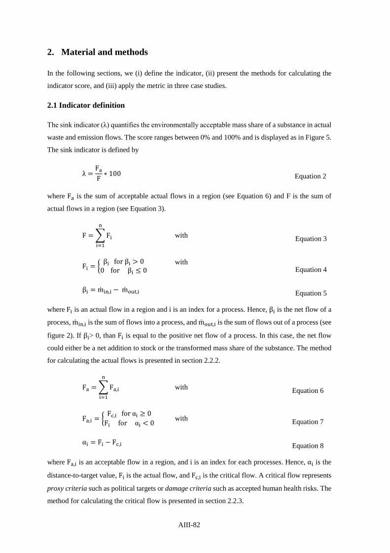
2. Material and methods
In the following sections, we (i) define the indicator, (ii) present the methods for calculating the
indicator score, and (iii) apply the metric in three case studies.
2.1 Indicator definition
The sink indicator (λ) quantifies the environmentally acceptable mass share of a substance in actual
waste and emission flows. The score ranges between 0% and 100% and is displayed as in Figure 5.
The sink indicator is defined by
λ =FaF∗ 100 Equation 2
where Fa is the sum of acceptable actual flows in a region (see Equation 6) and F is the sum of
actual flows in a region (see Equation 3).
F = �Fi
n
i=1
with Equation 3
Fi = � βi for βi > 00 for βi ≤ 0 with
Equation 4
βi = min,i − mout,i Equation 5
where Fi is an actual flow in a region and i is an index for a process. Hence, βi is the net flow of a
process, min,i is the sum of flows into a process, and mout,i is the sum of flows out of a process (see
figure 2). If βi> 0, than Fi is equal to the positive net flow of a process. In this case, the net flow
could either be a net addition to stock or the transformed mass share of the substance. The method
for calculating the actual flows is presented in section 2.2.2.
Fa = � Fa,i
n
i=1
with Equation 6
Fa,i = �Fc,i for αi ≥ 0
Fi for αi < 0 with Equation 7
αi = Fi − Fc,i Equation 8
where Fa,i is an acceptable flow in a region, and i is an index for each processes. Hence, αi is the
distance-to-target value, Fi is the actual flow, and Fc,i is the critical flow. A critical flow represents
proxy criteria such as political targets or damage criteria such as accepted human health risks. The
method for calculating the critical flow is presented in section 2.2.3.
AIII-82

Figure 1(a) shows the acceptable flow Fa,i as a function of the distance-to-target value αi. If αi < 0
then the actual flow Fi represents the acceptable flow Fa,i. If αi ≥ 0 then the critical flow Fc,i
represents the acceptable flow Fa,i. Figure 1(b) plots the actual flow Fi on both axes in combination
with the distant-to-target value αi. This produces three potential sub-flows: First, the acceptable
flow is the mass flow below the actual flow (for αi < 0) or below the critical flow (for αi ≥ 0).
Second, the unacceptable flow is the mass flow above the critical flow. Third, the tolerable flow is
the mass flow below the critical flow and above the actual flow. In other words, the tolerable flow
expresses the potential to increase the actual flow without violating normative criteria.
Figure 1 (a): Acceptable flow Fa,i as a function of the distant-to-target value αi. Example 1 demonstrates that for αi<0 the acceptable flow Fa,i is equal to the actual flow Fi. Example 2 demonstrates that for αi≥0 the acceptable flow Fa,i is equal to the critical flow Fc,i. Figure 1 (b): The combination of the actual flow Fi and the distant-to-target value αi yields two potential sub-flows: acceptable and unacceptable flows. Example 1 demonstrates for αi<0 the results of an acceptable flow. Example 2 demonstrates for αi≥0 the result of acceptable and unacceptable flows.
Figure 2: Plot of a generic process 𝑖𝑖, where ��𝑚𝑖𝑖𝑅𝑅,𝑖𝑖 is the substance flow [mass per time] entering process 𝑖𝑖, ��𝑚𝑅𝑅𝑜𝑜𝑠𝑠,𝑖𝑖 is the substance flow [mass per time] leaving process 𝑖𝑖, and ��𝑚𝑠𝑠𝑠𝑠𝑅𝑅𝑐𝑐𝑠𝑠,𝑖𝑖 is the resulting alteration of mass [mass/time] within process 𝑖𝑖.
2.2 Methods for calculating the indicator score
Fc,i Fi
Fa,i
Fc,i
αi<0 αi≥0
1 2
(a)
Fc,i Fi
Fi
Fc,i
αi<0 αi≥0
Acceptable flow
Unacceptable flow
Acceptable flow
1 2
(b)
AIII-83

To calculate the indicator score four steps are required (figure 3): First, the scope of assessment is
defined. Second, a descriptive assessment of flows yields the sum of actual flows F. Third, a
normative assessment of flows yields the sum of acceptable flows Fa. Fourth, the indicator score is
calculated.
Figure 3: Framework to calculate the indicator score.
2.2.1 Scope
Setting the scope of the assessment includes the selection of a substance, a reference region and a
period of interest. First, the notion “substance” is defined as “Matter of constant composition best
characterized by the entities (atoms, molecules, formula units) it is composed of” (Nic et al., 2012).
This is in line with the SFA framework used in this study, which defines the notion as “any
(chemical) element or compound composed of uniform units” (Brunner and Rechberger, 2004).
Second, the assessment deliberately focuses on regional flows instead of all flows along the life
cycle chain of products. A region is bounded by administrative limits. Accordingly, communities,
cities, federal states, nations or continents are subjects of the assessment. Third, setting the system
boundary in time includes the selection of a reference period (day, week, month, year, decade, and
so on) and a reference point in time (e.g. the year 2013). Temporal variations of flows within the
reference period are often neglected because of lack of data.
AIII-84

2.2.2 Descriptive assessment
To quantify the sum of actual flows F (equation 3), four steps are needed: First, to investigate into
the anthropogenic metabolism, SFA has been proven to be a practical tool. It tracks the pathway of
selected substances through systems such as households, enterprises, cities or regions. The applied
methodology is in accordance with Baccini and Bader (1996); Brunner and Rechberger (2004). The
model development focuses on the identification of relevant processes and their links in terms of
flows. Figure 4 present a framework for developing the SFA model. Model equations define the
flows and stocks with the help of input parameters. Next, balance equations are applied for each
process (figure 2, figure 4). The software STAN is used for data reconciliation and error propagation
in order to balance mass flows and stocks (Cencic, 2012). Second, Sankey-Diagrams are elaborated
to present SFA results (Schmidt, 2008). Third, the actual flows are determined. Therefore, the net
flow βi of each process (equation 5) is calculated and displayed. This kind of plot allows the
comparisons of various Sankey-Diagrams in a comparable manner. A positive net flow (βi>0)
indicates a sink process, and a negative net flow (βi<0) indicates a source process. The actual flow
Fi is defined as a positive net flow into a sub-process within the process “Waste management” and
“Environment” (equation 4). Fourth, the actual flows are summed up (equation 3).
Figure 4: The SFA model refers to a specific substance, region and period of time. It includes processes in the, production, trade and use phase, in the waste management sector, and in the environment. Flows link the processes. The flows assessed by the indicator λ include the actual flows within the flows “Waste”, “Emissions I”, and “Emissions II”.
For two out of the three case studies, we use SFA data that have already been published: Cu in
Vienna for the year 2008 (Kral et al., 2014) and PFOS in Switzerland for the year 2007 (Buser and
Morf, 2009). The third case study focuses on Pb in Vienna for the year 2008. Background datasets
can be found in the supplement information. In common, the Sankey-Diagram serves as starting
point for calculating the net flows βi and for filtering the actual flows Fi.
AIII-85

2.2.3 Normative assessment
To determine the acceptable flow Fa (equation 6), four steps are needed: First, normative criteria
and reference values define the acceptance of flows into sinks. Criteria and reference values are
derived from goal oriented frameworks with respect to waste and emissions, such as regulations,
standards, political agreements, or concepts for sustainable resource use like “clean cycles and final
sinks” (Brunner, 2010; Kral et al., 2013), and “gradle to gradle” (Mulhall and Braungart, 2010).
The definition of criteria depends on circumstances in the case study region. The circumstances
might change over time, for example, as a consequence of new scientific knowledge, by improved
data availability, and by changes in the ethical value-sphere. The circumstance might also vary from
region to region, for example, as a consequence of initiatives to increase the recycling rate, different
political agreements for accepted emission rates, and environmental quality standards. To select
normative criteria and reference values in a specific region, the outcome of stakeholders’
involvement might be considered, without being further discussed in this article. To consider
various criteria in the indicator framework, a criteria is related at any stage throughout the cause-
effect chain of a substance, and a reference value determines the normative criteria in a quantitative
manner. Table 2 gives some examples for proxy criteria at the stage of pressure, state, exposure and
effect, and damage criteria at the stage of damage. Second, the critical flows are calculated based
on models that establish causal links between the actual flow and the reference value attributed.
Hence, the actual flow Fi is varied as long as the reference value is achieved. The resulting flow is
called critical flow Fc,i. In the case of multiple criteria for a single actual flow, the most stringent
criteria is selected. Third, the distant-to-target value (equation 8) determines the acceptable flow
Fa,i (equation 7). Fourth, the acceptable flows are summed up (equation 6).
Table 2: Examples for normative criteria and reference values in context of the cause-effect chain, from the source towards the damage (adopted from Hofstetter 1998, Frischknecht 2009).
Stage Stage description Normative criteria Reference values Source Potential of waste and
emissions n.r. n.r.
Pressure Flow into sink Emission rates Waste into landfill
Legal limits, political agreements
State Substance fate in a) geogenic and b) anthropogenic sinks.
Substance concentration, accumulation or transformation rate in a) environmental media, and b) recycling goods, landfills, underground storage facilities.
Geogenic reference values in soil; Approved landfill capacity and disposal time;
Exposure Standard characteristics of exposed organism
Exposed dose, collective effective dose MAK values, BAT values
Effect Dose-Response-Relationship
Number and type of human diseases, Number of vanishing plant species
Accepted number of cases regarding an human disease
Damage Damage to human health or ecosystem quality
DALYs, QALYs, Share of vanishing plant species per area and time unit.
Value weighted DALYs, Accepted share of vanishing plant species per area and time unit
Notes: n.r. = not relevant; MAK values = Maximum Concentrations at the Workplace, BAT values = Biological Tolerance Values; DALY = disability-adjusted life years or disease-adjusted life years; QALY = quality adjusted life year;
AIII-86

In view of the case studies, the selection of normative criteria and references values is based on the
Ecological Scarcity (ES) method (Frischknecht et al., 2009) including the following adoptions:
• ES method provides critical flow data for Switzerland. We adopt the data according to local
circumstances in the case study region. For example, critical metal flows into surface waters
refer to local environmental quality standards for surface waters of the specific case study
country.
• ES method uses proxy criteria such as national reduction targets for greenhouse gas emissions
and legal standards for heavy metal concentrations in surface waters. In addition, we introduce
impact criteria such as human health risk. The integration of impact criteria demonstrates an
additional option for critical flow determination. For human health risk, the cancer risk level
(RL) and the non-cancer hazard-index (HI) represent two impact criteria.
• The ES method does not include PFOS as substance of interest. Legal limits in terms of
concentrations in various emission flows have not been published yet. To assess flows into
surface waters, we use an U.S. based reference concentration as proxy criteria.
• ES method assesses waste flows into landfills based on standards for the carbon content. We
replace this proxy criterion with the constraints given by the official permission for each
landfill. Therefore, the remaining landfill volume is divided by the approved, remaining time
for disposal. The conversion of the annual volume flow into mass yields the annual critical
flow into landfills.
• ES method aims at assessing impacts of waste and emission flows. Flows without impacts are
not taken into account. But, they are of concern for the applied method. For example, organic
substances are transformed mainly into carbon dioxide and water in incinerators, and are not
present in their original form anymore. Accordingly, we introduce proxy criteria for organic
substances in incineration. The critical flow is defined with the capacity of the incinerator in
mass per year.
The applied method is in line with ES methodology as follows:
• Heavy metals to soils: The Swiss Regulation on the Impact on Soils (Schweizer Bundesrat,
1998) aims to ensure long-term soil fertility. Accumulation of heavy metals in soil is not
accepted. ES method defines the critical flow as the heavy metal uptake through plants. This
simplified approach neglecting leaching from the soil might be justified due to a lack of more
precise regional data, but should be amended in the future.
• Hazardous waste to underground storage facilities: Switzerland has no appropriate storage
facilities and thus exports hazardous waste to foreign underground storages facilities. In
consultation with Swiss authorities, ES method sets the actual flow equal to the critical flow.
Just as Switzerland, Austria exports waste into underground storage facilities. This justifies
the same definition of the critical flow.
AIII-87

2.2.4 Indicator score
Applying descriptive and normative assessment methods result in an indicator score, ranging from
0% to 100% (Figure 5). The indicator takes 100% of actual flows into account, and discriminates
between acceptable and unacceptable flows. Either all actual flows are fulfilling criteria of
acceptability (λ=100%), at least one flow is unacceptable (0%<λ<100%), or all actual flows are
unacceptable (λ=0%). Accordingly, the positive connotation of the score can be seen as the more
the better.
Figure 5: Generic plot of the indicator score λ shows both, the amount of acceptable and unacceptable flows into sinks. The score refers to the total flows into sinks of a given substance, within a given region and within a given time period.
In general, the interpretation of the indicator score depends on the selection of (i) actual flows, (ii)
normative criteria and references values, and (iii) data availability.
The export flow “Exported waste & recycling material” crosses the spatial system boundary and
enters external regions (see figure 4). It might be that the flow is not acceptable due to local
circumstances in the export region, for instance, as a consequence of missing standards for pollution
control, a lack of environmental sound treatment and recycling facilities, and sanitary landfills. The
relevance of waste exports fraught with risk are well documented, for example, for waste electrical
and electronic and equipment (e.g. Sthiannopkao and Wong, 2013; Widmer et al., 2005). In view
of the present case studies, the flow “Exported waste & recycling material” is allocated to the
external region and not taken into account, except those into underground storage farcicalities. To
0%
100%
SubstanceRegionPeriod
Indi
cato
r sc
ore λ
[%]
Share of unacceptable flowsShare of acceptable flows
Actual scoreλ
Worst score
Best score
AIII-88

allocate flows into external sinks to the export region, critical flows for “Exported waste & recycling
material” have to be defined.
Normative criteria and reference values can be derived from goal oriented frameworks such as
regulations, standards, and political agreements. If the goals cannot be operationalized in terms of
normative criteria and reference values, or if criteria are not considered in the indicator score
calculation, the indicator score lacks of interpretational power regarding the goal oriented concepts.
For example, conclusions regarding the effectiveness of recycling initiatives fail, if a normative
criteria regarding recycling is missing. To overcome this gap, the critical flow into landfill might
be 10% lower than the actual flow, if the recycling rate should be enhanced by 10%.
Data acquisition is based on a bottom-up approach, supposing appropriate data quality and quantity.
If data is lacking, the outcomes point to data requirements that have to be met before implications
for environmental and waste management can be identified.
2.3 Case studies
The following three case studies are used to demonstrate the application of the sink indicator: Cu
in Vienna, Pb in Vienna, and PFOS in Switzerland (table 2). First, we highlight the motivation for
the case study selection and briefly explain the background. Second, we present detailed Sankey-
Diagrams including substance flows and calculate the sum of actual flows F according to Equation
3. Third, we calculate the critical flows in order to discriminate between acceptable and
unacceptable flows, respectively. The sum of acceptable flow yields Fa according to Equation 6.
Results are presented in table 3.
Table 3: Case study overview Substance Region Year Descriptive
method Number of actual flows
Number of sink processes
Type of criteria
SFA data reference
Cu Vienna 2008 SFA 8 4 Proxy criteria
Kral, Lin et al. (2014)
Pb Vienna 2008 SFA; EFM 9 7
Proxy and damage criteria
Supplement information
PFOS Switzerland 2007 SFA 6 5 Proxy criteria
Buser et al. (2009)
Notes: Cu = copper; Pb = lead; PFOS = perfluorooctanesulfonate; SFA = substance flow analysis; EFM = environmental
fate modeling;
AIII-89

2.3.1 Cu in Vienna
Copper is relevant from both a resource use and environmental impact viewpoint. On the one hand,
Cu is essential for modern lifestyles, resulting in Cu waste fractions that have to be disposed of.
From 1900-2000, about 0.7% of the Swiss Cu stock have been annually discarded in landfills
(Wittmer, 2006). On the other hand, Cu is emitted from point and non-point sources and poses a
risk for aquatic life. In Germany, it has been estimated that about 30% of total Cu loadings in
receiving waters originate from urban areas (Böhm et al., 2001). In Vienna, Cu concentrations in
sewage sludge are significantly larger than in rural areas (Kroiss et al., 2008), and Cu concentrations
in urban soils are higher than in surrounding rural areas (Pfleiderer, 2011).
The Sankey-Diagram in figure 6a represents the annual Cu flows for the city of Vienna for the year
2008. Details about the SFA study have been published by (Kral et al., 2014). Calculating the sum
of actual flows yields 1,129 t Cu/yr (figure 6b). Thereof, 97.3% are disposed of in a local landfill,
1.5% are shipped to a foreign underground storage facility, 0.8% are deposited on urban soil, and
0.4% are entering receiving waters.
To determine the critical flows, we use proxy criteria. The critical flow of bottom-ash into landfill
results from the available landfill volume of 3.45 million cubic meter, a density of 1.8 tons per cubic
meter, the approved remaining time for disposal with 19 year (Ableidinger et al., 2007), and the
actual Cu mass in bottom ash with 990 kg/yr. The critical flow for exported air-pollution-control
(APC) residues into an underground storage facility is set equal to the actual flow. This assessment
is justified, because the Viennese disposal practice meets the Swiss practice. The critical flow into
soil is taken as equal to the Cu uptake through plants, which has been calculated for green and
agricultural areas in Vienna (Kral et al., 2014). The critical flow into receiving water is based on
environmental standards for surface waters with 9.3 microgram Cu per liter (μg Cu/l )
(Bundesrepublik Österreich, 2006). There are two flows in total: The actual overflow from mixed
sewer system is 37.5 million tons of water per year (Leitner, 2013). The actual Cu concentration of
effluents from WTTP is 8.8 μg Cu/l (Kroiss et al., 2008).
Figure 6: (a) Sankey-Diagram for copper in Vienna for the year 2008. Annual flow rates and changes in stocks are given in tons per year (t/yr), for stocks in tons (t). The flows are represented as Sankey diagrams proportional to the flow rate; figures for stocks are given within the process boxes. Deviations from mass balance are due to rounding. (b) The Source-Sink-Diagram presents the net flows βi for each process i. The actual flows are positive net flows into the waste management sector and the environment. (c) The plot shows the results from normative assessment, namely the rated flows into sinks.
AIII-90

-30,000
-20,000
-10,000
0
10,000
20,000
30,000
Impo
rts
Indu
stry
, bus
ines
s &
serv
ices
Priv
ate
hous
ehol
ds
Tech
nica
l inf
rast
ruct
ure
Vehi
cles
Was
te c
olle
ctio
n, tr
ansp
ort
and
sepe
ratio
n
Inci
nera
tion
Land
fill
Und
ergr
ound
sto
rage
Was
te w
ater
col
lect
ion
&tre
atm
ent
Air
Wat
er
Soil
Expo
rtsProduction, trade & use Waste management Environment
Net
flow
βi[
t/yr]
0.1
1.0
10.0
100.0
1000.0
10000.0
Bottom-ash frommunicipal solid
waste incineration
APC residues fromMSW incineration
Stormwateroverflow from mixed
sewer system
Effluent from wastewater treatment
plant
DepositionFertilizer
PesticidesCompost
Landfill Undergroundstorage
Surface water Surface water Soil
Anthropogenic sinks Geogenic sinks
Cop
per f
low
[t/y
r]
Actual flow
Critical flow
Acceptable flow
(b)
(c)
Actual flows
(a)
AIII-91

2.3.2 Pb in Vienna
Human health is directly affected by emissions of Pb and Pb compounds. In Austria, Pb emissions
to air decreased from 218 t/yr in the year 1990 to 13 t/yr in 2009 (Anderl et al., 2011). In 1993, lead
has been banned from the Austrian petrol market. It is still used in accumulators, building coatings,
tires and paints. Due to former Pb depositions and present diffusive losses, anthropogenic Pb is
found in urban soils (Kreiner, 2004). Hence, it can be transferred to fodder and food, and may affect
human health (WHO, 2007). Up to now, the Pb content in Austrian soils lacks of systematic nation-
wide monitoring (Umweltbundesamt, 2010).
The Sankey-Diagram in figure 7a represents the annual Pb flows for the city of Vienna for the year
2008. Details about the SFA are given in the supplemental information. Calculating the sum of
actual flows yields the sum of actual flows with 191 t Pb/yr, of which 75.4% entered a local landfill,
22.9% entered a foreign underground storage facility, 0.8% entered ambient air, 0.5% entered urban
soil, and 0.3% entered receiving waters (figure 7b).
To determine the critical flows, we use (a) damage criteria for flows into geogenic sinks and (b)
proxy criteria for flows into anthropogenic sinks.
ad (a) The impact of flows into geogenic sinks is assessed in view of human health risks. Therefore,
we apply the risk assessment model CalTOX 4.0 beta (McKone and Enoch, 2002). CalTOX has
been developed to assess human exposures from continuous emissions to multiple environmental
media. Background datasets can be found in the supplemental information. The method quantifies
two damage criteria, namely the RL and the HI. To calculate the critical flows, we varied the actual
flows as long as the damage criteria result acceptable risks. To demonstrate the method, widely-
used acceptable risks of 10-6 for RL and 1 for HI are selected, without discussing further acceptable
risks (Kelly, 1991). Each actual flow is varied in a single scenario. Each variation results in two
critical flows. One meets the acceptable RL, another meets the acceptable HI. Accordingly, three
actual flows result in six scenarios. We picked out a stringent scenario, representing the minimum
ratio between the critical flow and the actual flow.
ad (b) Flows into anthropogenic sinks are determined with proxy criteria in accordance to the Cu
case study. The critical flow into landfills takes into account three different flows: Bottom ash from
incineration, excavated soil, and demolition waste. An average annual flow is calculated with
respect to landfill capacity. Therefore, the approved remaining landfill volume is divided by the
approved disposal time (Ableidinger et al., 2007). The flow into the foreign underground storage
facility is assessed in accordance with ES method. Therefore, the actual flow equals the critical
flow. This approach has been chosen because the Viennese disposal practice is equal to the Swiss
practice.
AIII-92

Figure 7: (a) Sankey-Diagram for lead in Vienna for the year 2008. Annual flow rates and changes in stocks are given in tons per year (t/yr), for stocks in tons (t). The flows are represented as Sankey diagrams proportional to the flow rate; figures for stocks are given within the process boxes. Deviations from mass balance are due to rounding. (b) The Source-Sink-Diagram presents the net flows βi for each process i. The actual flows are positive net flows into processes within the waste management sector and the environment. (c) The plot shows the results from normative assessment, namely the rated flows into sinks.
-2500
-2000
-1500
-1000
-500
0
500
1000
1500
2000
2500
Impo
rts
Indu
stry
, bus
ines
s &
serv
ices
Priv
ate
hous
ehol
d
Tech
nica
l inf
rast
ruct
ure
Vehi
cles
Was
te c
olle
ctio
n,tra
nspo
rt an
d se
pera
tion
Inci
nera
tion
Land
fill
Und
ergr
ound
sto
rage
Was
te w
ater
col
lect
ion
& tre
atm
ent
Air
Wat
er
Soil
Expo
rts
Production, trade & use Waste management Environment
Net
flow
βi[
t/yr]
0.11.0
10.0100.0
1000.010000.0
Bottom-ashfrom
municipalsolid wasteincineration
Excavatedsoil
Demolitionwaste
APC residuesfrom MSWincineration
Emissions Effluent fromwaste watertreatment
plantStormwater
overflow
Compost
Landfill I Landfill II Landfill III Undergroundstoragefacility
Air Surface water Soil
Anthropogenic sinks Geogenic sinks
Lead
flow
[t/y
r]
Actual flow
Critical flow
Acceptable flow
(b)
(c)
Actual flows
(a)
AIII-93

2.3.3 PFOS in Switzerland
Perfluorooctane sulfuric acid and its derivatives, collectively named PFOS, are persistent, bio-
accumulative and toxic substances. They are regulated under the Persistent Organic Pollutants
Regulation 850/2004 (European Parliament, 2004) and Regulation 2006/122/EG (European
Parliament, 2006). In 2010, PFOS has been added to the convention with some exemptions for
specific applications (European Commission, 2010). Hence, the European Union urges member
states to implement strategies for careful PFOS management.
In Switzerland, the Federal Office of the Environment conducted a national study regarding the
determination of stockpiles and waste fractions containing PFOS for the year 2007 (Buser and Morf,
2009). The corresponding Sankey-Diagram can be found in figure 8a. The production and use phase
as well as - in consequence of - the waste water treatment plant (WWTP) act as main PFOS sources.
Waste management provides the “anthropogenic sink” incineration, which mineralizes PFOS into
carbon dioxide, water and HF. Environment provides the geogenic sinks hydrosphere, soil and
atmosphere. Calculating the sum of actual flows yields 2,260 kg PFOS/yr, of which 77.1% entered
incineration, 0.4% entered landfills, and 22.5% entered geogenic sinks within hydrosphere,
atmosphere and soil (figure 8b). The flow from WWTP to hydrosphere is determined with a
concentration of 114 *10-9 gram PFOS per liter (ng/l) (Götz et al., 2011).
To determine the critical flows, we classified the actual PFOS flows into incineration as acceptable
flow. This is in accordance to the EU Regulation, because PFOS is mineralized if it undergoes
thermal treatment. Beyond the mineralized fraction, there is a very small PFOS fraction in
incineration ashes. Due to the large concentrations of heavy metals and certain organic refractory
substances, the ashes are classified as hazardous waste and are deposited in landfills or foreign
underground storage facilities. According to ES method, this actual flow is set equal to the critical
flow. This assessment is justified, because the Viennese disposal practice meets the Swiss practice.
For flows into geogenic sinks, there is a lack of normative criteria. To estimate the critical flow
from WWTP into surface waters, national standards are actually missing but under development
(Götz et al., 2011). We used the critical concentration of 200 ng/l PFOS. This value is a provisional
health advisory for drinking water, published by US EPA (2009). Due to the lack of regulations and
standards, other flows to the environment cannot be assessed and thus are excluded from normative
assessment.
Figure 8: (a) Sankey-Diagram for PFOS in Switzerland for the year 2007. Annual flow rates and changes in stocks are given in kilogram per year (kg/yr), for stocks in kilogram (kg). The flows are represented as Sankey arrows proportional to the flow rate; figures for stocks are given within the process boxes. Deviations from mass balance are due to rounding. (b) The Source-Sink-Diagram presents the net flows βi for each process i. The actual flows are positive net flows into processes within the waste management sector and the environment. (c) The plot shows the results from normative assessment, namely the rated flows into sinks.
AIII-94

-1500
-1000
-500
0
500
1000
1500
2000
Impo
rts
Fire
-figh
ting
foam
sto
rage
Appl
icat
ion
Serv
ice
life
End-
of-li
fe
Rec
yclin
g
Sew
erag
e
Inci
nera
tion
Was
te w
ater
trea
t. pl
ant
Land
fill
Wat
er Air
Soil
Expo
rts
Production, trade & use Waste management Environment
Net
flow
βi
[kg/
yr]
0.1
1.0
10.0
100.0
1000.0
10000.0
Solid waste &sewage sludge
Bottom-ashfrom municipal
solid wasteincineration
Effluent fromwaste water
treatment plant
Emissions fromother sources
Emissions Emissions
Incineration Landfill Surface water Surface water Soil Air
Anthropogenic sinks Geogenic sinks
PFO
S flo
w [t
/yr]
Actual flow
Critical flow
Acceptable flow
b) Actual flows
(c)
b)
AIII-95

3. Results
The following sections give an overview of the results, and discuss the composition of the indicator
score λ for each case study.
3.1 Overview
The indicator score λ for each case studies is visualized in figure 9. It quantifies the share of
acceptable flows in entire flows into sinks. The Cu metabolism in Vienna is limited by flows into
the geogenic sink urban soil and receiving waters. The PFOS metabolism in Switzerland partly
lacks of normative assessment due to lack of data, and the Pb metabolism in Vienna is restrained
by flows into anthropogenic sinks such as local landfills. To compute the indicator score, the sum
of acceptable and actual flows is needed and compiled in table 4.
Table 4: Substance flow data required for calculating the indicator score. Case study
Sink Flow Actual flow Fi [t/yr]
Critical flow
Fc,i [t/yr]
Acceptable flow
Fa,i [t/yr] Cu Landfill Bottom-ash from MSW incineration 1,097.2 2,075.5 1,097.2 Underground
storage facility APC residues from MSW incineration (exported filter cake) 16.4 16.4 16.4
Surface water Stormwater overflow from mixed sewer system 3.9 0.3 0.3
Surface water Effluent from WWTP 1.6 1.7 1.6 Soil Deposition, Fertilizer, Pesticides,
Compost 8.8 1.1 1.1
Sum F = 1,127.9 - Fa = 1,116.6 Pb Landfill I Bottom-ash from MSW incineration 94.7 198.5 94.7 Landfill II Excavated soil 17.3 4.3 4.3 Landfill III Demolition waste 31.9 29.8 29.8 Underground
storage facility APC residues from MSW incineration (exported filter cake)
43.9 43.9 43.9
Air Emissions 1.6 6.1 1.6 Surface water Stormwater overflow from mixed sewer
system Runoff from separated sewer system Effluent from WWTP
0.6 0.6 0.6
Soil Compost 1.0 1.0 1.0 Sum F = 190.9 - Fa = 175.8 PFOS Incineration Solid waste and sewage sludge 1.744 1.744 1.744 Landfill Bottom-ash from MSW incineration 0.009 0.009 0.009 Surface water Effluent from WWTP 0.420 0.737 0.420 Surface water Emissions from other sources 0.060 n.a. n.a. Soil Emissions 0.029 n.a. n.a. Air Emissions 0.001 n.a. n.a. Sum F = 2.263 - Fa = 2.173
Note: -=not relevant; n.a.=not available due to a lack of normative criteria; APC=Air pollution control; WWTP=Waste water treatment plant; t/yr=tons per year, Fa=sum of acceptable flows; F=sum of actual flows; Cu=copper, Pb=lead; PFOS=perfluorooctanesulfonate
AIII-96

Figure 9: Compilation of Indicator scores λ for the three case studies.
3.2 Cu in Vienna
99.0% of all actual Cu flows into sinks are acceptable. The sink “soil” poses a constraint for 0.7%
of all actual Cu flows only. The sink “surface water” poses a constraint for 0.3% of all actual Cu
flows. In detail, the following results have been obtained (figure 6c), whereas the percentage
numbers refer to the sum of actual Cu flows (100%≙1.128 t/yr):
• Landfill: 97.3% of flows are due to bottom-ash from MSW incineration. This is in
compliance with landfill regulation. Calculated by the approved volume and service time
of the landfill, the critical flow is 189% larger than the actual flow. Consequently, there is
no constraint for the disposal of bottom-ash until the end of the approved service time.
However, recycling is one option to disburden the landfill. If the stakeholders strive to
increase the recycling rate of bottom-ash, the indicator calculation has to include a criteria
with respect to both, the flow into the landfill and the recycled material flow (see chapter
2.2.4).
• Underground storage facility: 1.5% of flows are due to APC residues from MSW
incineration. These residues are exported and disposed of in approved underground storage
facilities.
• Water: 0.1% of flows are from effluents from WWTP, fulfilling quality standards for
surface waters. However, the actual flow is only 6% below the critical flow. Beside WWTP
effluents, Cu in stormwater overflow from mixed sewer systems enters receiving waters
too. Applying the same standards as for effluents shows that the actual flow is 11 times
99.0% 96.0% 92.1%
0%
100%
CopperVienna2008
PFOSSwitzerland
2007
LeadVienna2008
Indi
cato
r sco
re λ
[%]
Amount of actual flows without normative assessmentAmount of unacceptable flowsAmount of acceptable flows
AIII-97

larger than the critical flow. From an impact point of view, the flow complies with the
quality standards in the receiving water. For the future, the indicator score might increase
due to ongoing measures for reducing Cu bypassing waste water treatment via storm water
overflow. Retention reservoirs and collection sewers are constructed at present in order to
direct more urban surface waters including diffusive Cu losses towards WWTP (e.g. Stadt
Wien, 2013).
• Soil: 0.1% of flows are acceptable, and 0.7% of flows are unacceptable because they exceed
the critical level by a factor of eight. Cu flows into the soil are larger than the removal by
plants. If no Cu leaching from soil is assumed (cf. ES methodology), Cu will be
accumulating in specific soil compartments. The determination of the critical flow was
rather crude due to a lack of accurate local data. Consequently, the quantity and quality of
data has to be improved. This finding is in agreement with the recommendation of the
Austrian Environmental Agency for a nation-wide soil metal monitoring program
(Umweltbundesamt, 2010). Improved sampling with respect to horizontal and vertical
sample collection and including the identification of potential hot spots would allow
decreasing the uncertainty when determining the amount of unacceptable flows to the soil.
3.3 Pb in Vienna
92.1% of all actual Pb flows into sinks are acceptable. The sink “landfill” poses a constraint for
7.9% of all actual Pb flows. In detail, the following results have been obtained (figure 7c), whereas
the percentage numbers refer to the sum of actual Pb flows (100%≙191 t/yr):
• Landfills: 49.6% of flows is due to bottom-ash from MSW incineration. Due to the permit
of the landfill, the critical flow is twice as large as the actual flow. 15.9% of all actual Pb
flows originates from excavated soil to local landfills. If the landfill capacity should be
fully utilized at the end of approved disposal time, only 9.1% of all actual Pb flows (instead
of 15.9%) can be disposed of. The same pattern was found for Pb in demolition waste.
17.8% of Pb origins from demolition waste to landfills. If the landfill capacity should be
utilized at the end of approved disposal time, only 16.7% of all actual Pb flows (instead of
17.8) can be disposed of. If the disposal practice continues, landfills for excavated soil and
for demolition waste will exceed their approved landfill volume within the approved time
for disposal. In other words, the disposal of actual flows is in accordance with legal limits,
but the disposal practice faces constraints. To overcome these constraints, landfill
permissions have to be extended in time. Alternatively, waste fractions can be recycled
complying with advanced quality standards (BRV 2009), or wastes are directed to remote
landfills beyond the system limits, which increases transport distances and costs.
AIII-98

• Underground storage: 22.9% of flows originate from APC residues from MSW
incineration. The fractions are acceptable and exported into foreign underground storage
facilities.
• Air, soil, water: 0.8% of flows enter ambient air, 0.5% enters urban soil, and 0.3% enters
the water. The actual flows yield acceptable risks (RL: 7*10-6, HI: 0.26). Increasing the
actual flow into air by a factor of three results in a critical flow (HI: 1). Even though the
results yield acceptable human health risks, it has to be noted that the method is based on a
uniform approach without spatial resolution. Thus, accidental hot spots representing
possible risks for the local population are not included by this approach.
3.4 PFOS in Switzerland
96.0% of all actual PFOS flows into sinks are acceptable. 4% of all actual PFOS flows lack of
normative assessment due to insufficient knowledge. In detail, the following results have been
obtained (figure 8c), whereas the percentage numbers refer to the sum of actual PFOS flows
(100%≙2.260 t/yr):
• Incineration: 77.1% of PFOS flows are originating from solid waste and sewage sludge and
are treated by MSW incineration. This flow is mineralized and is classified as acceptable
flow, which is accordance to the EU Regulation (European Commission, 2010).
• Landfill: 0.4% of flows derives from residues of waste incineration and enters landfills in
an acceptable manner. Today’s PFOS emissions from landfills result from former rather
than from present waste disposal. They have been assessed too.
• Water: Two flows enter the aquatic sphere. 18.6% of PFOS are within WWTP effluents
and fulfill provisional drinking water standards (US EPA, 2009). Up to now in Switzerland,
legal limits are missing but under development (Götz et al., 2011). Even though standards
will be available in the future, the monitoring of PFOS is rather challenging and expensive
(e.g. Becker et al., 2008; Schultz et al., 2005). 2.7% of PFOS originate from additional
sources. This flow has not been assessed, because data and standards were missing.
• Soil and air: 1.3% of PFOS enter the soil, and 0.04% enter the air. These flows, together
with the 2.7% of flows into water have not been assessed. They pose potential threats on
human and ecological health without a clear understanding about the fate and effects.
AIII-99

4. Conclusions
A new methodology is presented to assess if sinks are a constraint for waste and emission flows.
The methodology is based on an indicator, ranging from 0% to 100%, and representing the ratio
between the amount of environmentally acceptable and unacceptable flows into sinks. To our
knowledge, it is the first indicator that indicates possible constraints for regional waste and emission
flows to sinks in a region-wide perspective. The methodology is tested by three case studies on Cu
and Pb in Vienna, and PFOS in Switzerland. The findings have several implications for material,
environmental and waste management: (i) As long as the indicator score stays below 100%, there
are unacceptable substance flows to geogenic and/or anthropogenic sinks. The information gained
while determining the new indicator is highly instrumental for developing strategies and measures
to decrease these flows and to raise the score up to a maximum value of 100%. (ii) The study shows
the important part waste management (incineration and landfilling) plays as a relevant and
necessary sink for anthropogenic material flows. (iii) For the three substances taken into account
by the case studies, there are fractions (roughly 1 to 10 %) that flow to inappropriate sinks. Still,
these flows can pose an environmental problem and should be further investigated
5. Outlook
The article starts with a statement, highlighting the constraints for anthropogenic carbon flows not
only at the supply but also at the disposal side. In the case of carbon, the United Nations Framework
Convention on Climate Change (UNFCCC) aims at managing the carbon content of the atmosphere.
So, nations periodically update and publish national inventories of anthropogenic carbon emissions
and removals by sinks. In the future, the systematic provision of source/sink inventories beyond
carbon facilitates informed decisions about substance flow management in a comprehensive
manner. This supports a sustainable resource management strategy with respect to safe sinks as
both, need and constraint for waste and emissions.
Acknowledgments
This study was supported by the Austrian Science Fund (FWF): I 549-N21 and the Taiwanese
National Research Council (NSC): NSC99-2923-E-002-006-MY3.
AIII-100

References
Abeles, F.B., Craker, L.E., Forrence, L.E., Leather, G.R., 1971. Fate of Air Pollutants: Removal
of Ethylene, Sulfur Dioxide, and Nitrogen Dioxide by Soil. Science 173, 914-916.
Ableidinger, M., Arbter, K., Hauer, W., Sciri, S., Volk, U., 2007. Wiener
Abfallwirtschaftskonzept 2007: Ist-Zustand der Wiener Abfallwirtschaft. Stadt Wien, Wien.
Alfsen, K., Sæbø, H., 1993. Environmental quality indicators: Background, principles and
examples from Norway. Environmental and Resource Economics 3, 415-435.
Anderl, M., Gangl, M., Göttlicher, S., Köther, T., Pazdernik, K., 2011. Emissionstrends 1990 -
2009 - Ein Überblick über die österreichischen Verursacher von Luftschadstoffen (Datenstand
2011). Umweltbundesamt.
Azar, C., Holmberg, J., Lindgren, K., 1996. Socio-ecological indicators for sustainability.
Ecological Economics 18, 89-112.
Baccini, P., Bader, H.P., 1996. Regionaler Stoffhaushalt. Spektrum, Akad. Verlag, Heidelberg,
Berlin, Oxford.
Becker, A.M., Gerstmann, S., Frank, H., 2008. Perfluorooctane surfactants in waste waters, the
major source of river pollution. Chemosphere 72, 115-121.
Berg, B., Dise, N., 2004. Calculating the long-term stable nitrogen sink in northern European
forests. Acta Oecologica 26, 15-21.
Berg, M., Scheringer, M., 1994. Problems in Environmental Risk Assessment and the need for
proxy measures. Fresenius Environmental Bulletin 3.
Böhm, E., Hillenbrand, T., Marscheider-Weidemann, F., Schempp, C., Fuchs, S., Scherer, U.,
2001. Bilanzierung des Eintrags prioritärer Schwermetalle in Gewässer, Berlin.
Brunner, P., 1999. In search of the final sink. Environmental Science and Pollution Research 6, 1-
1.
Brunner, P.H., 2010. Clean cycles and safe final sinks. Waste Management & Research 28, 575-
576.
Brunner, P.H., Rechberger, H., 2004. Practical Handbook of Material Flow Analysis. CRC Press
LLC, Boca Raton, Florida, U.S.
Brunner, P.H., Tjell, J.C., 2012. Do we need sinks? Waste Management & Research 30, 1-2.
AIII-101

BRV, 2009. Kurzfassung der Richtlinie für Recycling-Baustoffe. Baustoff Recycling Verband
(BRV), Wien.
Bundesrepublik Österreich, 2006. 96. Verordnung des Bundesministers für Land- und
Forstwirtschaft, Umwelt und Wasserwirtschaft über die Festlegung des Zielzustandes für
Oberflächengewässer, Wien.
Buser, A., Morf, L.S., 2009. Substance flow analysis for Switzerland: Perfluorinated surfactants
perfluorooctanesulfonate (PFOS) and perfluorooctanoic acid (PFOA), Environmental studies no.
0922, Bern, Switzerland.
Cencic, O., 2012. Software platform STAN (short for subSTance flow ANalysis). Vienna
Universtiy of Technology, Vienna.
Chen, W.-Q., Graedel, T.E., 2012. Anthropogenic Cycles of the Elements: A Critical Review.
Environmental Science & Technology 46, 8574-8586.
Döberl, G., Brunner, P.H., 2004. Substances and their (final) sinks - a new indicator for
monitoring sustainability, Indicators for Evaluating Sustainable Development - The Ecological
Dimension, Berlin, Germany.
EEA, 2012. Environmental indicator report 2012. European Environment Agency (EEA),
Copenhagen.
European Commission, 2010. Commission Regulation (EU) No 756/2010 of 24 August 2010
amending Regulation (EC) No 850/2004 of the European Parliament and of the Council on
persistent organic pollutants as regards Annexes IV and V.
European Parliament, 2004. Regulation (EC) No 850/2004 of the European Parliament and of the
Council of 29 April 2004 on persistent organic pollutants and amending Directive 79/117/EEC.
European Parliament, 2006. Directive 2006/122/ECof the European Parliament and of the Council
of 12 December 2006 amending for the 30th time Council Directive 76/769/EEC on the
approximation of the laws, regulations and administrative provisions of the Member States
relating to restrictions on the marketing and use of certain dangerous substances and preparations
(perfluorooctane sulfonates).
Feichter, J., 2008. Die Atmosphäre als Schadstoffsenke - Einfluss auf Stoffkreisläufe und Klima,
in: Gleich, A., Gößling-Reisemann, S. (Eds.), Industrial Ecology. Vieweg+Teubner, pp. 41-58.
Fong, D.P., Zedler, D.J.B., 2000. Sources, sinks, and fluxes of nutrients (N + P) in a small highly
modified urban estuary in southern California. Urban Ecosystems 4, 125-144.
AIII-102

Frischknecht, R., 2009. Skriptum zur Vorlesung: Umweltverträgliche Technologien - Analyse und
Beurteilung.
Frischknecht, R., Steiner, R., Jungbluth, N., 2009. The Ecological Scarcity Method – Eco-Factors
2006. A method for impact assessment in LCA., Bern.
Gilbert, A.J., Feenstra, J.F., 1994. A sustainability indicator for the Dutch environmental policy
theme ‘Diffusion’: cadmium accumulation in soil. Ecological Economics 9, 253-265.
Götz, C.W., Kase, R., Hollender, J., 2011. Mikroverunreinigungen - Beurteilungskonzept für
organische Spurenstoffe aus kommunalem Abwasser. Studie im Auftrag des BAFU, Dübendorf.
Grandjean, P., 2013. Science for precautionary decision-making, in: European Environmental
Agency (Ed.), Late lessons from early warnings: science, precaution, innovation. Publications
Office of the European Union, Luxembourg, pp. 623-642.
Graymore, M.L.M., Sipe, N.G., Rickson, R.E., 2010. Sustaining Human Carrying Capacity: A
tool for regional sustainability assessment. Ecological Economics 69, 459-468.
Guinée, J.B., van den Bergh, J.C.J.M., Boelens, J., Fraanje, P.J., Huppes, G., Kandelaars,
P.P.A.A.H., Lexmond, T.M., Moolenaar, S.W., Olsthoorn, A.A., Udo de Haes, H.A., Verkuijlen,
E., van der Voet, E., 1999. Evaluation of risks of metal flows and accumulation in economy and
environment. Ecological Economics 30, 47-65.
Henseler, G., Scheidegger, R., Brunner, P.H., 1992. Die Bestimmung von Stoffflüssen im
Wasserhaushalt einer Region. Vom Wasser 78, 91-116.
Hofstetter, P., 1998. Perspectives in life cycle impact assessment - A structured approach to
combine models of the technosphere, ecosphere and valuesphere. ETH Zürich, Zürich.
ICSU, 1989. The ocean as a source and sink for atmospheric trace constituents (Final report of
SCOR Working Group 72). International Council of Scientific Unions (ICSU), UNESCO, Paris.
ISWA, 2013. Sinks, a vital element of modern waste managment, in: Heiskanen, J. (Ed.), ISWA
Beacon, 2nd International Conference on Final Sinks. Aalto University, Espoo, Finnland.
Jungbluth, N., Büsser, S., Frischknecht, R., Flury, K., Stucki, M., 2012. Feasibility of
environmental product information based on life cycle thinking and recommendations for
Switzerland. Journal of Cleaner Production 28, 187-197.
Kelly, K.E., 1991. The Myth of 10-6 as a Definition of Acceptable Risk, 84th Annual Meeting Air
& Waste Management Association, Vancouver, B.C., Canada.
AIII-103

Kral, U., Kellner, K., Brunner, P.H., 2013. Sustainable resource use requires “clean cycles” and
safe “final sinks”. Science of The Total Environment 461–462, 819-822.
Kral, U., Lin, C.-Y., Kellner, K., Ma, H.-w., Brunner, P.H., 2014. The Copper Balance of Cities.
Journal of Industrial Ecology, in press, online available.
Kreiner, P., 2004. Wiener Bodenbericht 2003: Untersuchung des Wiener Bodens auf
Schwermetalle und polyaromatische Kohlenwasserstoffe. Stadt Wien, Wien.
Kroiss, H., Morf, L.S., Lampert, C., Zessner, M., 2008. Optimiertes Stoffflussmonitoring für die
Abwasserentsorgung Wiens. Technische Universität Wien, Wien.
Leitner, K., 2013. Water balance of Vienna as framework for a substance flow analysis of copper.
Vienna University of Technology, Vienna.
Loiseau, E., Junqua, G., Roux, P., Bellon-Maurel, V., 2012. Environmental assessment of a
territory: An overview of existing tools and methods. Journal of Environmental Management 112,
213-225.
Mackay, D., Shiu, W., Ma, K., Lee, S., 2006. Handbook of Physical-chemical Properties and
Environmental Fate for Organic Chemicals. Taylor & Francis Group, Boca Ration.
McKone, T.E., Enoch, K.G., 2002. CalTOX (registered trademark), A multimedia total exposure
model spreadsheet user's guide. Version 4.0(Beta). University of California, California.
Molina, M.J., Rowland, F.S., 1974. Stratospheric sink for chlorofluoromethanes: chlorine atomc-
atalysed destruction of ozone. Nature 249, 810-812.
Morf, L.S., Brunner, P.H., 2005. MVA als Schadstoffsenke - Stoffflussanalyse für Quecksilber im
MHKW Würzburg. Technische Universität Wien, Wien und Zürich.
Mulhall, D., Braungart, M., 2010. Cradle to Cradle. Criteria for the Built Environment, Nunspeet,
Netherlands.
Nic, M., Jirát, J., Kosata, B., Jenkins, A., 2012. Compendium of chemical terminology (Version
2.3.2). International Union of Pure and Applied Chemistry (IUPAC), Research Triangle Park, NC.
Nilsson, J., Bergström, S., 1995. Indicators for the assessment of ecological and economic
consequences of municipal policies for resource use. Ecological Economics 14, 175-184.
OECD, 2007. Measuring Material Flows and Resource Productivity. The OECD guide. OECD
Environment Directorate.
AIII-104

Ott, C., Rechberger, H., 2012. The European phosphorus balance. Resources, Conservation and
Recycling 60, 159-172.
Paterson, E., Sanka, M., Clark, L., 1996. Urban soils as pollutant sinks — a case study from
Aberdeen, Scotland. Applied Geochemistry 11, 129-131.
Pfleiderer, S., 2011. Umweltgeochemie Stadtgebiet Wien, Seminar Ressourcenmanagement und
Abfallwirtschaft, Wien.
Schmidt, M., 2008. The Sankey Diagram in Energy and Material Flow Management. Journal of
Industrial Ecology 12, 82-94.
Schnoor, J.L., 2013. Good news for peak emissions. Environ Sci Technol 47, 13209.
Schultz, M.M., Barofsky, D.F., Field, J.A., 2005. Quantitative Determination of Fluorinated Alkyl
Substances by Large-Volume-Injection Liquid Chromatography Tandem Mass Spectrometry -
Characterization of Municipal Wastewaters. Environmental Science & Technology 40, 289-295.
Schweizer Bundesrat, 1998. Verordnung vom 1. Juli 1998 über Belastungen des Bodens (VBBo).
Stadt Wien, 2013. Asperner Sammelkanal Entlaster in Bau, Wien.
Sthiannopkao, S., Wong, M.H., 2013. Handling e-waste in developed and developing countries:
Initiatives, practices, and consequences. Science of The Total Environment 463–464, 1147-1153.
Tarr, J.A., 1996. The search for the ultimate sink: urban pollution in historical perspective. The
university of Akron press, Akron.
Umweltbundesamt, 1999. Umweltindikatoren für Österreich - Regionale und nationale
Maßzahlen zur Dokumentation der Umweltsituation auf dem Weg zu einer nachhaltigen
Entwicklung, Umweltindikatoren für Österreich, Schloss Wilheminenberg, Wien.
Umweltbundesamt, 2010. Neunter Umweltkontrollbericht - Umweltsituation in Österreich, Wien.
UNCHS, 2001. The State of the Worlds Cities 2001. United Nations Centre for Human
Settlements (UNCHS), Nairobi.
UNCSD, 1996. Working List of Indicators of Sustainable Development. United Nations
Commission on Sustainable Development (UNCSD), New York.
UNEP, 2002. Regionally based assessment of persistent toxic substances. United Nations
Environment Programme (UNEP).
AIII-105
US EPA, 2009. Provisional Health Advisories for Perfluorooctanoic Acid (PFOA) and
Perfluorooctane Sulfonate (PFOS). U.S. Environmental Protection Agency (US EPA).
Van der Voet, E., 1996. Substances from cradle to grave: development of a methodology for the
analysis of substances flows through the economy and the environment of a region: with case
studies on cadmium and nitrogen compounds, Institute of Environmental Sciences. Leiden
University.
Vogg, H., 2004. Von der Schadstoffquelle zur Schadstoffsenke – neue Konzepte der
Müllverbrennung. Chemie Ingenieur Technik 60, 247-255.
WHO, 2007. Health risks of heavy metals from long-range transboundary air pollution. World
Health Organization (WHO), Copenhagen.
Widmer, R., Oswald-Krapf, H., Sinha-Khetriwal, D., Schnellmann, M., Böni, H., 2005. Global
perspectives on e-waste. Environmental Impact Assessment Review 25, 436-458.
Wittmer, D., 2006. Kupfer im regionalen Ressourcenhaushalt - Ein methodischer Beitrag zur
Exploration urbaner Lagerstätten. ETH Zürich, Zürich.
Yanai, R.D., Vadeboncoeur, M.A., Hamburg, S.P., Arthur, M.A., Fuss, C.B., Groffman, P.M.,
Siccama, T.G., Driscoll, C.T., 2013. From missing source to missing sink: long-term changes in
the nitrogen budget of a northern hardwood forest. Environ Sci Technol 47, 11440-11448.
Zeschmar-Lahl, B., 2004. Schadstoffverbringung in Senken durch Abfallbehandlung, Die
Abfallentsorgung auf der Zielgeraden. Abfallkolloquium 2004. Sächsisches Informations- und
Demonstrationszentrum Abfallbehandlungstechnologien,, Freiberg, pp. 71-104.
AIII-106

Supplement information for:
Kral, U, P.H. Brunner, P.C. Chen, S.R. Chen (2013). Sinks as limited resources? - A new
indicator for evaluating anthropogenic material flows. Ecological Indicators
Summary
This supplement information includes datasets for the case study about lead in Vienna. It comprises
the scope, the descriptive and normative assessment of lead flows. Figure 1 highlights the
framework to calculate the indicator score and the content of the supplement information in grey
colored boxes.
Figure 1: Framework to calculate the indicator score. Tasks documented within the supplement information are colored grey, including the section numbers. Tasks documented within the supplement information are dark grey colored.
Normative assessmentDescriptive assessment
ScopeSelection of substance, region, period (sec. 1)
Applying substance flow analysis (SFA) (sec. 2):• Identifying relevant processes & flows• Defining model equations, input parameters• Collecting data• Applying balance equations on each process
Determining actual flows:• Calculating net flows • Selecting actual flows• Visualizing results
Visualizing SFA results by the Sankey-Diagram (sec. 4.1, figure 5, 6)
Selecting normative criteria (sec. 3.1)
Proxy criteria
Applying risk assessment (sec. 3.2)
Damage criteria
Calculating critical flows (sec. 4.3)
Calculating distance-to-target values
Indicator score Calculating the indicator score λ
Summing up actual flows Summing up acceptable flows
Determining acceptable flows:• Calculating acceptable mass share of each actual
flow• Visualizing results
AIII-107

1 Scope
Lead is selected as substance of interest. The system boundary in space is set with the administrative
city limits. The system boundary in time is set with the year 2008.
2 Descriptive assessment
In the sections that follow, the calculation of actual lead flows is documented. First, the model
development includes the identification of processes and flows. Second, the model equations are
defined. Third, the flows are balanced using the software STAN.
2.1. Model development
The aim is to present a generic Pb flow model that allows the visualization of actual flows. This
requires an understanding of the key Pb flows in the city of Vienna. The determination of processes
and flows is based on previous studies, literature investigations, reports by local municipalities, and
expert interviews. The generic Pb flow model can be found in Figure 2 and Figure 3. The process
description is in accordance with Kral et al. (2013) and can be found in Table 1.
Figure 2: Generic lead flow model on top level. It covers 9 city internal processes of which 6 represent mainly anthropogenic activities (dark grey boxes) and 3 stand for environmental media (light grey boxes). Exterior processes are splitted in the supply and export as well as receiving waters in the hinterland. Regarding nomenclature, the flow acronyms refer to the type of flow (first three letters), to the source process (second three letters and to the sink process (last three letters). The stock acronyms refer to the type of stock only.
AIII-108

Figure 3: Generic lead flow model on 2nd level. It disaggregates the “Waste Management System”.
Table 1: Process characterization. Process name Characterization External anthroposphere Stands for the anthropogenic hinterland of the city. It delivers products and
construction material to the city and receives exported products, waste and recyclables.
Industry, business, services and forestry
Covers economic activities as well as related buildings. Economic activities refer to the trade of goods, material processing and distribution for final consumption. The buildings are addressed for stock calculation including construction material and installations.
Transport, energy, and communication infrastructure
Covers immobile infrastructure and corresponding lead stock in transport networks, power grids and telecommunication networks.
Vehicles Covers the mobile lead stocks such in cars, lorries, bikes, busses, trams, and trains. Private Households Covers anthropogenic activities of daily life and related buildings. Anthropogenic
activities refer to residing, nourishing, cleaning, and communication. Related buildings like flats and houses are used for stock calculation of construction material and installations.
Waste Management System Covers the collection, treatment and disposal of solid waste. The process is disaggregated which gives further insights into fluxes in view of incineration, composting and landfilling.
Waste Water Management System Covers the collection and treatment of waste water. Material stocks are not taken into account.
Underground storage External salt mines out of use act as final storage for hazardous residues from incineration.
Planetary boundary layer Stands for the lowest part of the atmosphere that is influenced by its contact with the earth surface, usually several hundred meters high.
Urban pedosphere and vegetation Consisting of urban soil and vegetation in parks, green areas and agricultural fields.
Urban hydrosphere Urban water bodies, mainly rivers, groundwater, ponds, and small lakes. Receiving waters The hydrosphere that takes up both, waste water treatment effluents and combined
sewer overflow from the city, such as the river Danube.
AIII-109

2.2 Model equations and data acquisition
This section provides a compilation of lead flow calculations. Table 2 includes the model equations
and the flow results, Table 3 includes all input parameters.
Table 2: Model Equations and flow results
AIII-110
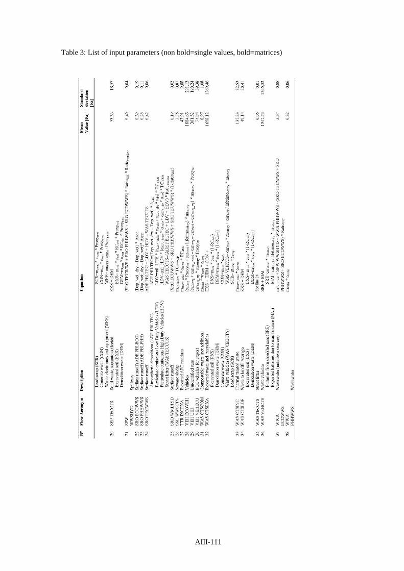
Table 3: List of input parameters (non bold=single values, bold=matrices)
AIII-111

AIII-112

AIII-113

AIII-114

2.3 Balance equations
The quantified flows from Table 2 do not fulfill the mass balance on each process. Consequently,
we balanced the flows by error propagation and data reconciliation. This step was carried out by
the software STAN (Cencic, 2012). The balanced flows are used to determine actual flows into
sinks (Table 5).
Table 4: Unbalanced versus balanced flows in t/yr.
Acronym Flow name Mass flow (unbalanced)
± Mass flow (unbalanced)
Mass flow (balanced)
± Mass flow (balanced)
ADE PBLECO Atmospheric deposition 0,17 0,03 0,17 0,03 ADE PBLPHH Atmospheric deposition 0,39 0,07 0,39 0,07 ADE PBLTEC Atmospheric deposition 0,23 0,04 0,23 0,04 ADE PBLUHY Atmospheric deposition 0,07 0,01 0,07 0,01 ADE PBLUPV Atmospheric deposition 0,73 0,12 0,73 0,10 COM COMUPV Compost as fertilizer 0,97 1,08 0,97 0,76 CON ECOPHH Construction material 0,00 0,00 0,00 0,00 CON ECOTEC Construction material 0,00 0,00 0,00 0,00
CON EXAECO Imported construction material 0,00 0,00 0,00 0,00
EFF WWSHYD Effluents 0,05 0,01 0,05 0,01 FER ECOUPV Fertilizer 0,00 0,00 0,00 0,00 HAR UPVECO Harvest 0,00 0,00 0,00 0,00 MSW ECOCTS Municipal solid waste 70,64 16,39 70,63 16,39 MSW PHHCTS Municipal solid waste 66,59 15,45 66,58 15,45 PAE ECOPBL Particulate emissions 1,13 0,08 1,13 0,07 PAE TECPBL Particulate emissions 0,00 0,00 0,00 0,00 PAE VEHPBL Particulate emission 0,40 0,12 0,40 0,10 PAE VEHTEC Particulate emissions 0,24 0,05 0,24 0,05 PAE WMSPBL Particulate emissions 0,06 0,01 0,06 0,01 PES UANUPV Pesticides 0,00 0,00 0,00 0,00 PRO ECOEXA Exported products 524,38 203,83 524,38 203,83 PRO ECOPHH Products & food 203,33 91,81 203,33 91,81 PRO EXAECO Imported products 2179,76 313,74 2179,76 313,74 RES INCLDF Residues 94,69 21,98 94,06 16,39
SEP ECOCTS Solid waste, separate collected 170,90 45,07 170,82 45,06
SEP PHHCTS Solid waste, separate collected 322,61 97,60 322,23 97,48
SEP TECCTS Solid waste, separate collected 53,36 18,57 53,35 18,57
SPW WWSHYD Spillway 0,40 0,04 0,40 0,04 SRO ECOWWS Surface runoff 0,39 0,07 0,39 0,07 SRO PHHWWS Surface runoff 0,23 0,04 0,23 0,04 SRO TECWWS Surface runoff 0,42 0,06 0,42 0,06 SRO WMIHYD Surface runoff 0,19 0,02 0,19 0,02 SSL WWSCTS Sewage sludge 3,75 0,87 3,92 0,62 TTR INCEXA Exported APC residues 43,91 9,88 43,78 9,43 VEH ECOVEH Vehicles 1804,65 291,13 1804,65 291,13 VEH UID Unidentified cars 361,52 190,24 361,52 190,24 VEH VEHECO EOL vehicles for export 74,84 39,38 74,84 39,38
WAS CTSCOM Compostable waste (net addition) 0,97 1,08 0,97 0,76
WAS CTSEXA Exported waste incl. recyclables 1698,12 1369,46 1772,92 968,58
WAS CTSINC Thermal treated waste 137,23 22,53 137,91 16,46 WAS CTSLDF Waste to landfill/storage 49,14 20,41 49,16 20,41 WAS TECCTS Street litter 0,05 0,01 0,05 0,01 WAS VEHCTS Waste vehicles 1347,74 1365,32 1273,39 968,56 WWA ECOWWS Wastewater 3,37 0,88 3,20 0,62 WWA PHHWWS Wastewater 0,32 0,06 0,32 0,06
AIII-115

3 Normative assessment
The sections that follow include the selection of the criteria, the methodology to calculate the
criteria, as well the data needed to apply the methodology.
3.1 Selection of criteria
To assess the actual flows into natural sinks, two impact indices are selected in view of human
health. The “risk level” stands for the carcinogenic risk and the “hazard-index” stands for the non-
carcinogenic risk.
3.2 Risk assessment
The sections that follow include a brief overview of the risk assessment approach and details about
the background data.
3.2.1 Approach
To compute the two impact indices, the software tool CalTOX 4.0 has been applied. The model has
been developed by Lawrence Berkeley National Laboratory. CalTOX is designed to run in
Microsoft Excel® and is available online (State of California, 2007). The CalTOX model structure
is visualized in Figure 5.The approach covers three steps in total, though methodological details
can be found in the user manual (University of California, 1994):
• First, multimedia transport simulation is used to compute the fate of lead in the
environment. The model turns out the result of substance flows and stocks in each
compartment when the system reaches an equilibrium state.
• Second, exposure assessment defines the relation between the environmental medium and
the exposure medium. The result is the “average daily dose rate” for each exposure route.
• Third, the impact indices were calculated with the dose-response relationship of lead.
Figure 4: CalTOX model structure (adopted from State of California, 1993; State of California,
2007). It consist of (a) multimedia transport simulation, (b) exposure assessment, and (c) the risk
algorithm that yields two impact indices.
AIII-116

3.2.2 Data acquisition
In general, CalTOX requires four types of input data. The points that follow include the abbreviation
from the default values, provided by the CalTOX spreadsheet.
1. Emission flows in mol/day. These data are provided by the SFA model. Therefore, 1,59 t
Pb/yr enter air, 0,97 t Pb/yr enter soil and 0,64 t Pb enter water (sec. 2, Table 17).
Table 5: Anthropogenic flows for CalTOX model inputs Flow short name Flow name
Sink Actual flow
[ton/year]
Actual flow into sink
[ton/year]
Actual flow into sink* [mol/day]
PAE ECOPBL Particulate emissions Air 1,12 1.59 21.02 PAE VEHPBL Particulate emission Air 0,41
PAE WMSPBL Particulate emissions Air 0,06 COM COMUPV Compost as fertilizer Soil 0,97 0.97 12.81 EFF WWSHYD Effluents Water 0,05
0.64 8.50 SPW WWSHYD Spillway Water 0,40 SRO WMIHYD Surface runoff Water 0,19
Note: *=Conversion factor from [ton/year] to [mol/day]: 106[g/t] * 1mol/207.21 [g*t] * 1 [year/365days]
2. Chemical properties. In total 36 parameters are needed. Default values for Pb are provided
in CalTOX and used to run the model.
3. 58 landscape properties. In total 58 parameters are needed. 11 out of 58 landscape
parameters are adopted for Vienna (Table 18). 47 out of 58 parameters are default values,
provided in CalTOX, and were used to run the model.
4. Exposure factors. In total 52 parameters are needed.21 out of 52 exposure factors are adopt-
ed for Vienna (Table 19). 31out of 52 exposure factors are default values, provided in Cal-
TOX, and were used to run the model.
Table 6: Vienna's landscape properties in CalTOX Landscape properties Variable name value
Contaminated area in m2 Area 414871000
Annual average precipitation (m/d) rain 0.002
Land surface runoff (m/d) runoff 0.0008
Atmospheric dust load (kg/m3) rhob_a 2.39E-08
Ground-water recharge (m/d) recharge 0.00003
Thickness of the ground soil layer (m) d_g 0.01
Soil particle density (kg/m3) rhos_s 1600
Water content in surface soil (vol fraction) beta_g 0.15
Fraction of land area in surface water f_arw 0.05
Ambient environmental temperature (K) Temp 285
Yearly average wind speed (m/d) v_w 319200
AIII-117

Table 7: Vienna's exposure properties in CalTOX Human Exposure Factors Variable name value
Body weight (kg) BW 74
Surface area (m2/kg) SAb 0.0254
Fluid Intake (L/kg-d) Ifl 0.0208
Fruit and vegetable intake (kg/kg-d) Ifv 0.0055
Grain intake (kg/kg-d) Ig 0.0000
Milk intake (kg/kg-d) Imk 0.0095
Meat intake (kg/kg-d) Imt 0.0021
Egg intake (kg/kg-d) Iegg 0.0004
Fish intake (kg/kg-d) Ifsh 0.0002
Soil ingestion (kg/d) Isl 0.0002
Fraction of water needs from ground water fw_gw 0.0251
Fraction of water needs from surface water fw_sw 0
Frctn frts & vgtbls that are exposed produce fabv_grd_v 0.4
Fraction of fruits and vegetables local flocal_v 0.364
Fraction of grains local flocal_g 0.069
Fraction of milk local flocal_mk 0
Fraction of meat local flocal_mt 0
Fraction of eggs local flocal_egg 0
Fraction of fish local flocal_fsh 0
Exposure duration (years) ED 30
Averaging time (days) AT 28878.8
AIII-118

4 Results
The sections that follow include the Sankey-Diagram for actual flows, the actual risk based on the
actual flows, and the critical flows in view of acceptable risks.
4.1 Sankey-Diagram
Figure 5: The Sankey diagram for lead in Vienna on an annual base for the year 2008. Flow rates
and changes in stocks are given in mass/time, for stocks in mass. The flows are represented as
Sankey arrows proportional to the flow rate; figures for stocks are given within the process boxes.
AIII-119

Figure 6: The Sankey diagram for lead in the Viennese waste management sector, on an annual
base for the year 2008. Flow rates and changes in stocks are given in mass/time, for stocks in mass.
The flows are represented as Sankey arrows proportional to the flow rate; figures for stocks are
given within the process boxes.
4.2 Actual risks
The actual flows into natural sinks yield a risk level of 7.41 E-8(Carcinogenic risk) and a hazard-
index of 0.26 (non-carcinogenic risk). Table 20 and Table 21 shows that the risk level and the
hazard-index are mainly driven by the ingestion of lead due to vegetables grown above the ground
(exposed produce).
Table 8: The analysis of carcinogenic risk Exposure route Risk Contribution rate Inhalation 1.25 E-8 16.82% Ingestion 6.15 E-8 83.01%
Water 1.34 E-9 1.81% Exposed produce 6.01 E-8 81.03% Unexposed produce 2.54 E-14 0.00% Meat 0 0%
Milk 0 0%
Eggs 0 0%
Fish 0 0%
Soil 1.23 E-10 0.17% Dermal 1.33 E-10 0.18% Total Risk 7.41 E-8 100%
AIII-120

Table 9: The analysis of hazard-index Exposure route Hazard-index Contribution rate Inhalation 1.83E-02 6.98% Ingestion 2.43E-01 92.82%
Water 5.30E-03 2.03%
Exposed produce 2.37E-01 90.61%
Unexposed produce 1.00E-07 0.00%
Meat 0 0%
Milk 0 0%
Eggs 0 0%
Fish 0 0%
Soil 4.87E-04 0.19%
Dermal 5.24E-04 0.20%
HQ 2.62E-01 100%
4.3 Critical flows
Scenario 4 yields the minimum ratio between the critical flow and the actual flow (Table 22 and
Table 23).
Table 10: Critical flows in view of the risk level. Scenario
N° Sink Actual flow (tons/year)
Critical flow (tons/year)
Tolerable flow (tons/year)
Ratio critical / actual flow
1 Air 1,59 21,93 20,34 14 Water 0,64 0,64 0,00 Soil 0,97 0,97 0,00
2 Air 1,59 1,59 0,00 Water 0,64 461,35 460,74 717 Soil 0,97 0,97 0,00
3 Air 1,59 1,59 0,00 Water 0,64 0,64 0,00 Soil 0,97 2.647,11 2.646,14 2.733
Table 11:Critical flows in view of the hazard-index.
Sink Actual flow (tons/year)
Critical flow (tons/year)
Tolerable flow (tons/year)
Ratio critical / actual flow
4 Air 1.59 6.13 4.54 4 Water 0.64 0.64 0.00 Soil 0.97 0.97 0.00
5 Air 1.59 1.59 0.00 Water 0.64 90.76 90.15 141 Soil 0.97 0.97 0.00
6 Air 1.59 1.59 0.00 Water 0.64 0.64 0.00 Soil 0.97 605.05 604.08 625
References
AIII-121

AgPU, 2004. Produktions-, Verbrauchs-und Abfalldaten für PVC in Deutschland unter
Einbeziehung der Verwertung [Data about production, consumption and waste generation for
PVC in Germany]. Arbeitsgemeinschaft PVC und Umwelt (AgPU), Bonn.
BMLFUW, 2002a. Behandlungs- und Verwertungswege für PVC-Abfälle [Treatment and
disposal routes for PVC waste]. Wien.
BMLFUW, 2002b. Stand der Technik bei Abfallverbrennungsanlagen [State of the art of waste
incineration plants]. Bundesministerium für Land- und Forstwirtschaft, Umwelt und
Wasserwirtschaft (BMLFUW), Wien.
BMLFUW, 2011a. Bundes-Abfallwirtschaftsplan 2011 [Federal Waste Management Plan 2011].
Bundesministerium für Land- und Forstwirtschaft, Umwelt und Wasserwirtschaft (BMLFUW),
Wien.
BMLFUW, 2011b. Bundes-Abfallwirtschaftsplan 2011 (Band 2) [Federal Waste Management
Plan 2011 (part 2)]. Bundesministerium für Land- und Forstwirtschaft, Umwelt und
Wasserwirtschaft (BMLFUW), Wien.
Cencic, O., 2012. Software platform STAN (short for subSTance flow ANalysis). Url:
www.stan2web.net, Access date: 28th September 2012. Vienna Universtiy of Technology,
Vienna.
EAK, 2009. Tätigkeitsbericht 2008 [Annual Report 2008]. Elektroaltgeräte Koordinierungsstelle
Austria GmbH (EAK), Wien.
EMPA, 2009. Material composition. Url: http://ewasteguide.info/material_composition, Access
date: 25th August 2012. Eidgenössische Materialprüfanstalt, Dübendorf.
Fenz, R., 1999. Gewässerschutz bei Entlastungsbauwerken der Mischkanalisation [Water
protection of buildings regarding combined sewer systems]. PhD thesis, Technische Universität
Wien, Wien.
Forum Nachhaltiges Bauen, 2013. Blei - Ökobilanz [Lead - Life cycle assessment]. Url:
http://www.nachhaltiges-bauen.de/baustoffe/Blei, Access date: 1st October 2013. Forum
Nachhaltiges Bauen.
Haider, T., Haider, M., Wruss, W., Sommer, R., Kundi, M., 2002. Lead in drinking water of
Vienna in comparison to other European countries and accordance with recent guidelines.
International Journal of Hygiene and Environmental Health 205, 399-403.
Holzapfel, P., Riedel, R., 2011. Verkehrsmodell Wien [Traffic model Vienna]. Personal
communication, reicipent: Kellner, K., retrieved on 4th December 2011.
AIII-122

Hulskotte, J.H.J., Schaap, M., Visschedijk, A., 2006. Brake wear from vehicles as an important
source of diffuse copper pollution. Conference: 10th Int. Specialised Conference on Diffuse
Pollution ans Sustainable Basin Management, 18th - 22nd September 2006, Instanbul.
I C Consultants Ltd, 2001. Pollutants in Urban Waste Water and Sewage Sludge. European
Communities, Luxembourg.
Kalina, M., Leder, K., Kramer, S., Puxbaum, H., 2000. Nasse Deposition im Land Wien Oktober
99 - September 00 [Wet deposition in Vienna, Oktober 99 - September 00]. Technische
Univeristät Wien. Institut für Analytische Chemie. Abteilung für Umweltanalytik, Wien.
König, S., 2006. Stoffflussbasiertes Verfahren zur Bestimmung von Metallfrachten in Abfällen
[Methods to determine metal flows in waste]. Master thesis, Technische Universität Wien, Wien.
Kral, U., Lin, C.-Y., Kellner, K., Ma, H.-w., Brunner, P.H., 2013. The copper balance of cities:
Exploratory insights into a European and an Asian city. Journal of Industrial Ecology. in press.
Kroiss, H., Morf, L.S., Lampert, C., Zessner, M., 2008. Optimiertes Stoffflussmonitoring für die
Abwasserentsorgung Wiens [Optimized substance flow monitoring of the waste water treatment
plant in Vienna]. Technische Universität Wien, Wien.
Kronberger, R., 2011. Solid waste Inputs to Viennese incinerators 2008. Personal communication,
reicipent: Kral, U., retrieved on 21st November 2011, Wien.
Lampert, C., Stark, W., Kernbeis, R., Brunner, P.H., 1997. Stofffflussanalyse der
Siedlungsentwässerung der beiden Regionen "Gresten" und "Grafenwörth", Studie im Rahmen
des Niederösterreichischen Klärschlammkonzeptes [Susbtance flow analysis of regional water
discharge]. Technische Universität Wien, Wien.
Lebhart, G., 2010. Statistisches Jahrbuch der Stadt Wien 2010 [Statistical Yearbook of Vienna
2010]. Magistrat der Stadt Wien, Magistratsabteilung 5 - Finanzwesen, Wien.
Lehmann, T., 2011. Wastewater input into Viennas waste water system, ratio of mixed/separated
sewer system in Vienna. Personal communication, reicipent: Kellner, K., retrieved on 20th July
2011, Wien.
Luhana, L., Sokhi, R., Warner, L., Mao, H., Boulter, P., 2004. Characterisation of Exhaust
Particulate Emissions from Road Vehicles (PARTICULATES). Deliverable 8: Measurement of
non-exhaust particulate matter. Hatfield, UK.
Magistratsabteilung 05, 2011. Aussenhandelsstatistik für Wien 2008 [Trade Statistic for Vienna
2008, restricted for public access]. Personal communication, reicipent: Kral, U., retrieved on 5th
March 2012, Wien.
AIII-123

Morf, L.S., Taverna, R., 2006. Monitoringkonzept zur Ermittlung von Ursachen für
Veränderungen der Schwermetallgehalte im Wiener Restmüll [Monitoring concept to investigate
the change in heavy metal concentrations in residual waste of Vienna]. GEO Partner AG
Umweltmanagement, Zürich.
Reisinger, H., Jakl, T., Quint, R., Schöller, G., Müller, B., Riss, A., Brunner, P.H., 2009.
Ressourcenpotenzial und Umweltbelastung der Schwermetalle Blei, Cadmium und Quecksilber in
Österreich. in: Jakl, T. (Ed.), CHEM-NEWS XVIII. Bundesministerium für Land- und
Forstwirtschaft, Umwelt und Wasserwirtschaft, Wien, pp. 56-64.
Spiegel, H., 2003. Atmospheric deposition of heavy metals onto arable land in Austria.
Conference: Concerted Action AROMIS, 24th - 25th November 2003, Kloster Banz, Germany.
State of California, 1993. CalTOX, A Multimedia Total Exposure Model For Hazardous-Waste
Sites. Part I: Executive Summary. California.
State of California, 2007. CalTOX Download Instructions. Url:
www.dtsc.ca.gov/AssessingRisk/ctox_dwn.cfm, Access date: 25th March 2012. California.
Statistik Austria, 2008. Kraftfahrzeuge - Bestand [Number of registered vehicles]. Url:
www.statistik.at/web_de/statistiken/verkehr/strasse/kraftfahrzeuge_-_bestand/index.html, Access
date: 3rd August 2011. Wien.
Statistik Austria, 2009a. Kfz-Gebrauchtzulassungen 2008 [Number of re-registred cars 2008].
Url: www.statistik.at, Access date: 1st March 2012. Wien.
Statistik Austria, 2009b. Kfz-Neuzulassungen Jänner bis Dezember 2008 [Number of new
registered vehicles]. Url: www.statistik.at, Access date: 8th February 2012. Wien.
Statistik Austria, 2012. Bevölkerung Österreichs 2001-2050 nach Haushaltsgröße [Austrian
Inhabitants 2001-2050]. Url:
www.statistik.at/web_de/statistiken/bevoelkerung/demographische_prognosen/haushalts_und_fa
milienprognosen/023535.html, Access date: 1st May 2012. Wien.
Taverna, R., Rolland, C., Böker, C., Kirchner, A., 2011. Routinemäßiges Stoffflussmonitoring auf
der MVA Spittelau - Messperiode 1.5.09-30.4.10 [Routine monitoring measaures of the
incinerator Spittelau in Vienna - monitoring period: 1.5.09-30.4.10]. GEO Partner AG,
Magistratsabteilungen 22 und 48 der Stadt Wien, Fernwärme Wien GmbH, Zürich.
Tomenendal, A., 2011. Freshwater Supply Vienna. Personal communication, reicipent: Kellner,
K., retrieved on 19th July 2011.
Umweltbundesamt, 2000. Qualität von Komposten aus der getrennten Sammlung – Ergebnisse
der Kompostanalysen [Qualtity of compost from seperated collection]. Umweltbundesamt
Österreich, Wien.
AIII-124

University of California, 1994. CalTOX™, A Multimedia Total Exposure Model For Hazardous-
Waste Sites - Spreadsheet User’s Guide. California.
USDA, 2011. National Nutrient Database. Url: www.nal.usda.gov/fnic/foodcomp/search/, Access
date: 25th November 2011. U.S. Department of Agriculture (USDA).
VDZ, 1996. Umweltverträglichkeit von Zement und Beton [Environmental impact of cement and
concrete]. Verein Deutscher Zementwerke (VDZ), Düsseldorf.
Weinmar, K., 2011. Kompostproduktion und -verbrauch in Wien [Compost production and
consumption in Vienna]. Personal communication, reicipent: Kellner, K., retrieved on 2nd August
2010.
Westerlund, K.G., 2001. Metal emissions from Stockholm traffic - wear of brake linings.
Stockholm.
Wiener Umweltschutzabteilung MA22, 2011. Abfallstatistik Wien 2008 [Waste statistic for
Vienna 2008]. Personal communication, reicipent: Kellner, K., retrieved on 30th June 2011,
Wien.
Winther, M., Slento, E., 2010. Heavy metal emissions for danish road transport. NERI Technical
Report no. 780. Aarhus University, Aarhus, Denmark.
Wirtschaftskammer Österreich, 2012. Rahmendaten - Importe und Exporte gebrauchter Fahrzeuge
[Data about imports and exports of second life cars]. Url:
http://wko.at/fahrzeuge/main_frame/statistik/JB/Seite5.11%202012.pdf, Access date: 9th August
2012.
Woisetschlaeger, G., Musser, S., Lindlbauer, A., Wruss, W., 2000. Bestandsaufnahme der
Bodenbelastung in Wien PAK, KW, Schwermetalle [Assessement of soil contamination in
Vienna]. Magistratsabeilung 22, Wien.
AIII-125