A New Implementationof the Meshless Finite Volume Method ...
24
Copyright c 2004 Tech Science Press CMES, vol.6, no.6, pp.491-513, 2004 A New Implementation of the Meshless Finite Volume Method, Through the MLPG “Mixed” Approach S. N. Atluri 1 , Z. D. Han 1 and A. M. Rajendran 2 Abstract: The Meshless Finite Volume Method (MFVM) is developed for solving elasto-static problems, through a new Meshless Local Petrov-Galerkin (MLPG) “Mixed” approach. In this MLPG mixed approach, both the strains as well as displacements are interpolated, at randomly distributed points in the domain, through lo- cal meshless interpolation schemes such as the mov- ing least squares(MLS) or radial basis functions(RBF). The nodal values of strains are expressed in terms of the independently interpolated nodal values of displace- ments, by simply enforcing the strain-displacement rela- tionships directly by collocation at the nodal points. The MLPG local weak form is then written for the equilib- rium equations over the local sub-domains, by using the nodal strains as the independent variables. By taking the Heaviside function as the test function, the local domain integration is avoided; this leads to a Meshless Finite Vol- ume Method, which is a counterpart to the mesh-based finite volume method that is popular in computational fluid dynamics. The present approach eliminates the ex- pensive process of directly differentiating the MLS inter- polations for displacements in the entire domain, to find the strains, especially in 3D cases. Numerical examples are included to demonstrate the advantages of the present methods: (i) lower-order polynomial basis can be used in the MLS interpolations; (ii) smaller support sizes can be used in the MLPG approach; and (iii) higher accuracies and computational efficiencies are obtained. keyword: Meshless Local Petrov-Galerkin approach (MLPG), Finite Volume Methods, Mixed Methods, Ra- dial Basis Functions (RBF), and Moving Least Squares (MLS). 1 University of California, Irvine Center for Aerospace Research & Education 5251 California Avenue, Suite 140 Irvine, CA, 92612, USA 2 Army Research Office, RTP, NC 1 Introduction The meshless methods have been found to be attractive, mainly due to the possibility of overcoming the draw- backs of mesh-based methods, such as the labor-intensive process of mesh-generation, locking, poor derivative so- lutions, etc. The meshless methods may also eliminate the mesh distortion problems once the solid/structure un- dergoes large deformations, in which case, adaptive re- finement and adaptive remeshing are required. Several meshless methods have been developed, based on global weak forms, such as the smooth particle hydrodynamics (SPH), and the element-free methods and so on. They require certain meshes or background cells [over the so- lution domain, for purposes of integration of the weak- form], which may also become distorted during large deformations. In contrast, the meshless local Petrov- Galerkin (MLPG) approach pioneered by Atluri and his colleagues [Atluri (2004)] is based on writing the lo- cal weak forms of PDEs, over overlapping local sub- domains. The integration of the weak-form is also per- formed within the local sub-domains; thus negating any need for any kind of meshes or background cells, mak- ing the MLPG approach a truly meshless method. The MLPG approach has been used to solve various problems successfully, including those in elasto-statics [Li, Shen, Han and Atluri (2003); Han and Atluri (2003ab,2004a)], elasto-dynamics [Han and Atluri (2004b)], fracture me- chanics [Atluri, Kim and Cho (1999)], and fluid mechan- ics [Lin and Atluri (2001)] and so on. All these suc- cesses demonstrate that the MLPG method is one of the most promising alternative methods for computational mechanics. As a general framework for meshless methods, the MLPG approach provides the flexibility in choosing the trial and test functions, as well as the sizes and shapes of local sub-domains, and employs various[unsymmetric or symmetric] weak forms of PDEs. As a special case, the Heaviside function can be chosen as the test function,
Transcript of A New Implementationof the Meshless Finite Volume Method ...
Copyright c© 2004 Tech Science Press CMES, vol.6, no.6, pp.491-513, 2004
A New Implementation of the Meshless Finite Volume Method, Through theMLPG “Mixed” Approach
S. N. Atluri1, Z. D. Han1 and A. M. Rajendran2
Abstract: The Meshless Finite Volume Method(MFVM) is developed for solving elasto-static problems,through a new Meshless Local Petrov-Galerkin (MLPG)“Mixed” approach. In this MLPG mixed approach, boththe strains as well as displacements are interpolated, atrandomly distributed points in the domain, through lo-cal meshless interpolation schemes such as the mov-ing least squares(MLS) or radial basis functions(RBF).The nodal values of strains are expressed in terms ofthe independently interpolated nodal values of displace-ments, by simply enforcing the strain-displacement rela-tionships directly by collocation at the nodal points. TheMLPG local weak form is then written for the equilib-rium equations over the local sub-domains, by using thenodal strains as the independent variables. By taking theHeaviside function as the test function, the local domainintegration is avoided; this leads to a Meshless Finite Vol-ume Method, which is a counterpart to the mesh-basedfinite volume method that is popular in computationalfluid dynamics. The present approach eliminates the ex-pensive process of directly differentiating the MLS inter-polations for displacements in the entire domain, to findthe strains, especially in 3D cases. Numerical examplesare included to demonstrate the advantages of the presentmethods: (i) lower-order polynomial basis can be used inthe MLS interpolations; (ii) smaller support sizes can beused in the MLPG approach; and (iii) higher accuraciesand computational efficiencies are obtained.
keyword: Meshless Local Petrov-Galerkin approach(MLPG), Finite Volume Methods, Mixed Methods, Ra-dial Basis Functions (RBF), and Moving Least Squares(MLS).
1 University of California, Irvine Center for Aerospace Research &Education5251 California Avenue, Suite 140Irvine, CA, 92612, USA
2 Army Research Office, RTP, NC
1 Introduction
The meshless methods have been found to be attractive,mainly due to the possibility of overcoming the draw-backs of mesh-based methods, such as the labor-intensiveprocess of mesh-generation, locking, poor derivative so-lutions, etc. The meshless methods may also eliminatethe mesh distortion problems once the solid/structure un-dergoes large deformations, in which case, adaptive re-finement and adaptive remeshing are required. Severalmeshless methods have been developed, based on globalweak forms, such as the smooth particle hydrodynamics(SPH), and the element-free methods and so on. Theyrequire certain meshes or background cells [over the so-lution domain, for purposes of integration of the weak-form], which may also become distorted during largedeformations. In contrast, the meshless local Petrov-Galerkin (MLPG) approach pioneered by Atluri and hiscolleagues [Atluri (2004)] is based on writing the lo-cal weak forms of PDEs, over overlapping local sub-domains. The integration of the weak-form is also per-formed within the local sub-domains; thus negating anyneed for any kind of meshes or background cells, mak-ing the MLPG approach a truly meshless method. TheMLPG approach has been used to solve various problemssuccessfully, including those in elasto-statics [Li, Shen,Han and Atluri (2003); Han and Atluri (2003ab,2004a)],elasto-dynamics [Han and Atluri (2004b)], fracture me-chanics [Atluri, Kim and Cho (1999)], and fluid mechan-ics [Lin and Atluri (2001)] and so on. All these suc-cesses demonstrate that the MLPG method is one of themost promising alternative methods for computationalmechanics.
As a general framework for meshless methods, theMLPG approach provides the flexibility in choosing thetrial and test functions, as well as the sizes and shapes oflocal sub-domains, and employs various[unsymmetric orsymmetric] weak forms of PDEs. As a special case, theHeaviside function can be chosen as the test function,

492 Copyright c© 2004 Tech Science Press CMES, vol.6, no.6, pp.491-513, 2004
and applied to the symmetric-weak forms over the localsub-domains; thus eliminating the domain integrals [la-beled as MLPG-5Atluri and Shen (2002)]. It has a clearphysical meaning that the local weak form represents themomentum balance law of the local sub-domains. Thisis very similar to the finite volume methods, which havebeen widely used in computational fluid mechanics. Thefinite volume methods are usually second-order accurate,based on the integral form of the governing equations,over the non-overlapping sub-domains. The MLPG5method leads to what may be called as the “Meshless Fi-nite Volume Methods [MFVM]. With the use of iterativesolvers, the finite volume methods are more efficient totreat the coupling and non-linearity in an iterative way. Inrecent years industrial computational fluid dynamics hasbeen dealing with the meshes of the order of up to 100million cells. The smooth particle hydrodynamics (SPH)uses the so-called particles, interacting with each otherthrough the meshless approximations [Lucy (1977); Gin-gold and Monaghan (1977)]. Since the standard SPHmethod has the problem to interpolate exactly when theparticles are unevenly spaced and sized, many improve-ments were made to improve the completeness of theSPH approximation, such as the normalization [Johnsonand Beissel (1996)] and the MLS approximation [Dilts(1999)].
The problems of similar scale also exist in structural anal-ysis, especially for those undergoing the large nonlineardeformations under high-speed impact loading as in thecase of a projectile penetration problem. It is well knownthat this has been beyond the capability of the traditionalfinite element methods, due to the mesh problems and thepoor accuracy of the second-order variables. For exam-ple, in projectile penetration simulations, Johnson, Stryk,Beissel, and Holmquist (2002) used a SPH based algo-rithm to convert extremely distorted finite elements intoparticles to alleviate eroding (dropping) element massfrom the calculation and to avoid solution time steps be-coming extremely small. The MFVM described in thispaper may offer a viable alternative for this class of prob-lems.
In the present work, a new meshless finite volumemethod [MFVM] is developed for solving elasto-staticproblems, through an MLPG “mixed” approach. TheHeaviside function is used as the test function, inthe local-weak-form of the equilibrium equation. In-dependent meshless approximations are used for both
the strains, as well as the displacements. The strain-displacement compatibility is enforced at nodal points byusing the collocation method; thus expressing the inde-pendent nodal strains in terms of nodal displacements.These strains are then used in the local symmetric weak-form of the equilibrium equations. It retains the samephysical meaning as the momentum balance law of thelocal sub-domains, while the accuracy of the secondaryvariables has been improved. Theoretically, the presentmethod requires that the trial functions possess only C0continuity. In contrast, C1 continuities are required forthe trial functions if the derivatives of the displacementsare directly used in the weak-form. Numerically, thestrains are interpolated directly via the meshless approx-imations, without the calculation of the derivatives ofthe shape functions. The MLPG mixed method is thuscomputationally more efficient, because the calculationof the derivatives of the interpolation functions in themeshless approximations, everywhere in the vdomain,is computationally costly. In addition, the second-orderpolynomial bases are required for the better approxima-tion, to avoid shear-locking if the MLS is used [Hanand Atluri (2004a)], in the primal MLPG method (basedonly on displacement interpolations) Also in the MLPGprimal method, a larger support size should be chosen,in order to make the MLS approximation non-singular,which leads to over-smoothed results. The present mixedmethod requires only a first-order polynomial basis in theMLS approximations of both strains as well as displace-ments. A smaller support size can be used in the presentMLPG mixed method, and the number of nodes is re-duced dramatically, especially for 3D cases. The localintegrals in the present method contain only the strains,without involving the derivatives of the displacement ex-plicitly. Thus, the present MFVM method, based on theMLPG mixed approach, is more suitable for non-linearproblems with large deformations.
The main body of the paper begins with a brief descrip-tion of the augmented RBF, and MLS approximations inSection 2. The MLPG finite volume method is formu-lated in Section 3. The numerical implementation withthe pseudo codes is presented in Section 4. Numericalexamples are given in Section 6, and the conclusions anddiscussions are given in Section 7.
A New Implementation of the Meshless Finite Volume Method 493
2 Meshless Approximations
This section summarizes, for the sake of completeness,the meshless approximations for the MLPG methods, in-cluding the radial basis functions (RBF) and the movingleast squares (MLS). More details can be found in [Atluri(2004)].
The MLS method of interpolation is generally consideredto be one of the best schemes to interpolate random datawith a reasonable accuracy, because of its completeness,robustness and continuity. With the MLS, the distributionof a function u in Ωs can be approximated, over a numberof scattered local points xi, (i = 1,2, ...,n), as,
u(x) = pT (x)a(x) ∀x ∈ Ωs (1)
where pT (x) = [p1(x), p2(x), ... , pm(x)] is a monomialbasis of order m; and a(x) is a vector containing coef-ficients, which are functions of the global Cartesian co-ordinates [x1,x2,x3], depending on the monomial basis.They are determined by minimizing a weighted discreteL2 norm, defined, as:
J(x) =m
∑i=1
wi(x)[pT(xi)a(x)− ui]2
≡ [P ·a(x)− u]T W[P ·a(x)− u] (2)
where wi(x) are the weight functions and uiare the ficti-tious nodal values.
One may obtain the shape function as,
u(x) = pT (x)A−1(x)B(x)u≡ ΦΦΦT (x)u ∀x ∈ ∂Ωx (3)
where matrices A(x) and B(x) are defined by
A(x) = PT WP B(x) = PT W ∀x ∈ ∂Ωx (4)
The weight function in Eq. (2) defines the range of in-fluence of node I. Normally it has a compact support. Afourth order spline weight function is used in the presentstudy.
The radial basis functions (RBF) approximation pos-sesses the Dirac delta function property of the shapefunctions, and leads to a simplicity of their derivatives.However, they lack completeness, as in the standardSPH. It has been improved by introducing additionalpolynomials, as the augmented RBF. The RBF approxi-mation is globally continuous only for the case when the
approximation is also global. The shape functions arenon-continuous if they are used locally [Han and Atluri(2004a)].
Consider a sub-domain Ωs, the neighborhood of a pointx, which is local in the solution domain. To approxi-mate the distribution of function u in Ωs, over a numberof scattered points xi, (i = 1,2, ...,n), the local aug-mented RBFs interpolate u(x) of u, ∀x ∈ Ωs can be de-fined by [Golberg, Chen and Bowman (1999)]
u(x) = RT (x)a+PT (x)b ∀x ∈ Ωs (5)
where RT (x) = [R1(x),R2(x), ...,Rn(x)] is a set ofradial basis functions centered around the n scat-tered points; aT = [a1,a2, ...,an] is a vector of con-stant coefficients; PT (x) = [p1(x), p2(x), ... , pm(x)] =[1,x,y, z,x2,y2, z2,xy,yz, zx, ....] is a monomial basis of or-der m; bT = [b1,b2, ...,bm] is a vector of constant coeffi-cients. The radial basis function has the following gen-eral form
Ri (x) = Ri (ri) and ri = ‖x−xi‖ (6)
To determine the coefficients a and b, one may enforcethe interpolation to satisfy the given values at the scat-tered points, as:
u(xi) = RT (xi)a+PT (xi)bi = 1,2, ...,n or
ue = R0a+P0b (7a)
and
n
∑i=1
p j(xi)ai = 0 j = 1,2, ...,m or PT0 a = 0 (7b)
By solving Eq. (7), and substituting the solution into Eq.(5), one may obtain the shape function as:
u(x) =[RT (x),PT (x)
]Gue ≡ ΦΦΦT (x)ue ∀x ∈ Ωs (8)
where the matrix G is defined as:
G ≡[
R0 P0
PT0 0
]−1
(9)
In the present study, the compactly supported RBFs areused in a local way, and chosen as the weight functionused in the MLS.

494 Copyright c© 2004 Tech Science Press CMES, vol.6, no.6, pp.491-513, 2004
3 MLPG Finite Volume Method and Numerical Dis-cretization
Consider a linear elastic body in a 3D domain Ω, with aboundary ∂Ω, shown in Figure 1. The solid is assumedto undergo infinitesimal deformations. The equations ofbalance of linear and angular momentum can be writtenas:
x
sΩ
Figure 1 : A local sub-domain around point x
σi j, j + fi = 0; σi j = σ ji; (),i ≡ ∂∂ξi
(10)
where σi j is the stress tensor, which corresponds to thedisplacement field ui; fi is the body force. The corre-sponding boundary conditions are given as follows,
ui = ui on Γu (11a)
ti ≡ σi jn j = t i on Γt (11b)
where ui and t i are the prescribed displacements and trac-tions, respectively, on the displacement boundary Γu andon the traction boundary Γt , and ni is the unit outwardnormal to the boundary Γ.
In the MLPG approaches, one may write a weak formover a local sub-domain Ωs, which may have an arbitraryshape, and contain the a point x in question. A gener-alized local weak form of the differential equation (10)over a local sub-domain Ωs, can be written as:∫
Ωs
(σi j, j + fi)vidΩ = 0 (12)
where ui and vi are the trial and test functions, respec-tively.
By applying the divergence theorem, Eq. (12) may berewritten in a symmetric weak form as [Han and Atluri(2004a)]:∫
∂Ωs
σi jn jvidΓ−∫
Ωs
(σi jvi, j − fivi)dΩ = 0 (13)
Imposing the traction boundary conditions in (11), oneobtains∫
Ls
tividΓ+∫
Γsu
tividΓ+∫
Γst
tividΓ
−∫
Ωs
(σi jvi, j − fivi)dΩ = 0 (14)
where Γsu is a part of the boundary ∂Ωs of Ωs, over whichthe essential boundary conditions are specified. In gen-eral, ∂Ωs = Γs ∪ Ls, with Γs being a part of the localboundary located on the global boundary, and Ls is theother part of the local boundary which is inside the solu-tion domain. Γsu = Γs∩Γu is the intersection between thelocal boundary ∂Ωs and the global displacement bound-ary Γu; Γst = Γs ∩Γt is a part of the boundary over whichthe natural boundary conditions are specified.
Therefore, a local symmetric weak form (LSWF) in lin-ear elasticity can be written as:∫
Ωs
σi jvi, jdΩ−∫
Ls
tividΓ−∫
Γsu
tividΓ
=∫
Γst
t ividΓ+∫
Ωs
fividΩ (15)
One may use the Heaviside function as the test functioninj the local symmetric weak form in Eq. (15), and ob-tain,
−∫
Ls
tidΓ−∫
Γsu
tidΓ =∫
Γst
tidΓ+∫
Ωs
fidΩ (16)
Eq. (16) has the physical meaning that it represents thebalance law of the local sub-domain Ωs, with the tractionboundary conditions being enforced [Atluri (2004); Li,Shen, Han, and Atluri (2003)].
With the constitutive relations of an isotropic linear elas-tic homogeneous solid, the tractions in Eq. (16) can bewritten in term of the strains:
ti = σi jn j = Ei jklεkln j (17)
where,
Ei jkl = λδi jδkl +µ(δikδ jl +δil δ jk) (18)
A New Implementation of the Meshless Finite Volume Method 495
with λ and µ being the Lame’s constants.
Consider a local sub-domain Ωs, centered on each nodalpoint x(I); then the approximation of traction vectors onthe boundary of Ωs can be expressed by considering thenodal strains as independent variables. With the use ofthe shape function in Section 2, the strains are indepen-dently interpolated, as,
εkl(x) =N
∑K=1
Φ(K)(x)ε(K)kl (19)
With Eqs. (17) and (19), one may discretize the localsymmetric weak-form of Eq. (16), as,
−N
∑K=1
[∫
Ls
Φ(K)(x)Ei jkln jdΓ] ε(K)kl
−N
∑K=1
[∫
Γsu
Φ(K)(x)Ei jkln jdΓ] ε(K)kl
=∫
Γst
t idΓ+∫
Ωs
fidΩ (20)
It clearly shows that no derivatives of the shape functionsare involved in the local integrals. Instead, if Eq. (20)is written in terms of the displacement variables, theseintegrals will involve the derivatives of the shape func-tions [Atluri (2004)]. It is well known that the meshlessapproximation is not efficient in calculating such deriva-tives everywhere in the domain, especially when theMLS approximation is used. Thus, the efficiency of thepresent method is improved over the traditional MLPG[primal] displacement methods. Secondly, the require-ment of the completeness and continuity of the shapefunctions is reduced by one-order, because the strains,which are the secondary field variables, are approximatedindependently of the displacements. Thus, lower-orderpolynomial terms are required in the meshless approxi-mations, and a smaller nodal influence size can be cho-sen, to speed up the calculation of the shape functions.On the other hand, the number of equations in Eq. (20)is less than the number of the independent strain vari-ables, because the nodal strain variables are more thanthe displacement ones[ in 3D, there are six nodal-strainvariables, but only 3 displacement nodal-variables]. Onemay reduce the number of the variables by transform-ing the strain variables back to the displacement variablesvia the collocation methods, without any changes to Eq.(20). First, the interpolation of displacements can also be
accomplished by using the same shape function, for thenodal displacement variables, and written as,
ui(x) =N
∑J=1
Φ(J)(x)u(J)i (21)
For linear elasto-statics, the strain-displacement relationsare:
εkl =12(uk,l +ul,k) (22)
The standard collocation method may be applied to en-force Eq. (22) only at each nodal point x(I), instead ofthe entire solution domain. Thus, the nodal strain vari-ables are expressed in terms of the nodal displacementvariables, as
εkl(x(I)) =12[uk,l(x(I))+ul,k(x(I))] (23)
With the displacement approximation in Eq. (21), thetwo sets of nodal variables can be transformed through alinear algebraic matrix:
ε(I)kl = H(I)(J)
klm u(J)m (24)
where the transformation matrix H is banded.
The number of system equations is then reduced to thesame number as the nodal-displacement variables, afterthe transformation. In addition, such a transformation isperformed locally, and the system matrix retains its band-edness. For numerical implementation, it is not neces-sary to calculate and store the matrix H explicitly. Theintegrals in Eq. (20) are only related to a few nodal pointswhich are near to the point of interestion, x(I), whichmeans only a very small portion of the transformationmatrix H is used. It is possible to calculate this portionfrom Eq. (24) dynamically, which is less computation-ally costly with only a few local nodal points involved.
With the meshless approximations, another problem isthat the essential boundary conditions can not be imposeddirectly even with the use of the RBF approximation, be-cause the shape function possesses the Dirac delta prop-erty only at the corresponding nodes. Although one mayimpose the essential boundary conditions at all nodes onthe prescribed displacement boundary, these conditionsare still not satisfied everywhere on the boundary, exceptat the nodal points. The reason is that the boundary val-ues everywhere on the boundary, even through the RBF

496 Copyright c© 2004 Tech Science Press CMES, vol.6, no.6, pp.491-513, 2004
approximation, depend not only on the boundary nodes,but also on the related ones inside the domain. This isquite different from those in the element-based methods,in which the boundary values are interpolated throughonly the nodes at the boundary nodes. In the presentstudy, the collocation method is also used to impose thedisplacement boundary conditions. For a nodal point x(I),if its ith displacement DOF belongs to the displacement
boundary, i.e., u(I)i ∈Γsu, the corresponding system equa-
tion can be replaced by the one generated from the collo-cation for this particular DOF, as
αui(x(I)) = αui(x(I)) (25)
This standard collocation still keeps the system equationssparse and banded.
It should be pointed out that the present method is for-mulated based on the nodal points fully within the localsub-domains, as shown in Eqs. (20), (24) and 4. It makesthe present method ready for parallel computation andwork with iterative solvers or for solving transient im-pact problems [Han and Atluri (2004b)].
4 Numerical Implementation
Several numerical aspects are discussed in this section,mainly focusing on the issues in numerical implementa-tion and related techniques. The pseudo codes in MAT-LAB are given in each topic. Even though all algorithmsare demonstrated for 2D problems in this section, theyare extendable for the 3D cases, quite easily.
4.1 Data Preparation
Although only the scattered nodal points are requiredin the meshless method, it is not efficient to define theboundaries for a complicated domain. The easiest wayis to use the robust Delaunay algorithm to triangulate thesolution domain into triangles. These triangles are onlyused to define the solution domain and have no qualityrequirement, because they are not used for the interpola-tion or the integration. The steps in Table 1 are used toprepare the data for any general problems.
4.2 Quadrature Techniques
In the present method, the tractions are involved in theintegrals, which need to be evaluated over the boundaryof the local sub-domains. Polynomial termas for the trac-tion can not be expected over the entire local boundary,
sΩ
)(
0
Ir
)( Ix
)1(x
)2(x
)3(x
)4(x
)5(x
)4(y
)1(y
)2(y
)3(y
)5(y
Figure 2 : a local sub-domain around point x
which may not be covered by all local nodes. In addi-tion, the integrals contain the normal n to the bound-ary, and the trigonometric functions are involved. Itis well known that the conventional numerical quadra-ture schemes are designed for polynomials, but are notefficient for trigonometric functions [Han and Atluri(2004)]. For 2D problems, the numerical errors may becontrolled by simply increasing the order of the Gaussquadrature scheme, or subdividing the domain of integra-tion into small segments for better accuracy. It has beenreported that the subdivision algorithm is much more ef-ficient, than in the case when the integration is performedover the entire domain with a large number of integrationpoints [Atluri, Kim and Cho (1999), Sellountos and Poly-zos (2003)]. For those nodes on the global boundary, theintersection between the local and global boundaries alsoneeds some special treatment. In the present implemen-tation, a simple subdivision algorithm is used to simplifythe numerical quadrature and improve the accuracy.
Consider a local circular sub-domain centered at node I,x(I), with a radius denoted by r(I)
0 . By drawing a line fromnode I to its neighbor node J, x(J), (J = 1,2, ...,m), apoint can be obtained at the intersection between the lineand the local circle, denoted by y(J), (J = 1,2, ...,m).A subset of these intersecting points is used to dividethe integration domain, i.e. the local circle. It shouldbe pointed out that the intersection points between thelocal and global boundaries are automatically includedin y(J). Then these special points are kept in the sub-set and used as the starting and ending points. A set ofangles is obtained for performing the numerical integra-

A New Implementation of the Meshless Finite Volume Method 497
Table 1 : Sample codes for data preparation
i) read model data
load ‘node.dat’ node; % node contains the node coordinates in rows, as % [ x1, y1; x2, y2; … ; xn yn]
load ‘element.dat’ element; % element contains the triangles in rows, as % […; n1_Ti, n2_Ti, n3_Ti; …]
numnode=size(node,1); % number of nodes numelem=size(element,1); % number of triangles
ii) search the global boundary
% mlpgedge contains the definition of the global boundary % with anti-clock-wise node pairs in rows, as % [… … … ; n1_of_Pi, n2_Pi; … …]
mlpgedge = setdiff( ... [element(:,[1 2]);element(:,[2 3]);element(:,[3 1])], ... [element(:,[2 1]);element(:,[3 2]);element(:,[1 3])], ... 'rows'); clear element; % the triangles are removed after searching the global boundary
iii) search neighbor nodes
% mlpgnode contains the neighbor node information in rows, as % [… … ; m, I, n1, n2, … n_m-1;… …] % where m is the number of the neighbor node of node I, include node I itself.
supportSize = 2.05; % the radius of the nodal influence domain testSize = 0.55; % the radius of the local sub-domain
mlpgnode = zeros(numnode,1); for i=1:numnode d =sqrt((node(:,1)-node(i,1)).^2 + (node(:,2)-node(i,2)).^2); neighNode = find(d < supportSize+testSize); mlpgnode(i,1:size(neighNode,1)+1) = [size(neighNode,1) i setdiff(neighNode,[i])']; endclear d neighNode;
tion, as θ0, θ1, · · · , θt. The starting angle θ0 is notequal to the ending angle θt for the nodes on the globalboundary. In the present study, the radii of the local sub-domains for the nodes within the solution domain are sochosen that the local sub-domains do not intersect withthe global boundary. Thereafter, the subdivided anglescover the entire local circle for these internal nodes. Thesubdivision is illustrated in Figure 2.
In addition, the subdivision can also be used to divide thelocal sub-domain in pie slices with node I as the center,
if domain integrals are required, such as the body forces.Then, all the integrals over the local sub-domain can becalculated by using the simple Gaussian quadrature.
The codes in Table 2 are used to determine the local sub-division.
4.3 Post Processing
For the MLS approximation, the fictitious nodal valuesare obtained after solving the system equations. A simpleprocedure in Table 3 is used to calculate the actual nodal

498 Copyright c© 2004 Tech Science Press CMES, vol.6, no.6, pp.491-513, 2004
Table 2 : Sample codes for quadrature techniques
i) search the starting and ending angles for the nodes on the global boundary
% mlpgangle contains the starting and ending angles for all nodes % [… … … ; starting_angle_of_Node_I, ending_angle_of_Node_I; … …] % -inf and inf are used, respectively, for the internal nodes
mlpgangle = zeros(numnode,2); dr = node(mlpgedge(:,2),:) - node(mlpgedge(:,1),:); % length of all boundary edges % calculate the angles of the boundary edges % and used as the starting angle of the first node of the edge mlpgangle(mlpgedge(:,1),1) = cart2pol(dr(:,1),dr(:,2)); mlpgangle(find(mlpgangle>pi-eps),1)=-pi; % remove the numerical tolerance
% reverse the angle of the boundary edges, % and used as the ending angle of the second node of the edge mlpgangle(mlpgedge(:,2),2) = pi+mlpgangle(mlpgedge(:,1),1);
% regularize the starting and ending angles da = mlpgangle(:,2)-mlpgangle(:,1); ii = find(da > 2*pi); mlpgangle(ii,2) = mlpgangle(ii,2)-2*pi; ii = find(da < 0); mlpgangle(ii,1) = mlpgangle(ii,1)-2*pi;
ii = setdiff([1:numnode]', mlpgedge(:,1)); % set -inf & inf for all internal nodes mlpgangle(ii,1) = -inf; mlpgangle(ii,2) = inf; clear dr da ii;
ii) sub-divide the local circle
% mlpgnode contains the sub-divided angles for integration % [… … … ; number_of_angles, sita_0, sita_1, …, sita_t; … …]
f0 = linspace(0,1,9)'; % the maximum number of the angles is set to 10 for i=1:numnode ii = mlpgnode(i,3:mlpgnode(i,1)); % neighbor nodes excluding itself sita = cart2pol(node(ii,1)-node(i,1),node(ii,2)-node(i,2)); % all intersecting angles
startangle = max(mlpgangle(i,1),min(sita)); ii = find(sita <startangle); sita(ii) = sita(ii)+2*pi;
endangle = min(startangle+2*pi,mlpgangle(i,2)); sita = sita(find(sita <=endangle)); [f,sita] = ecdf(sita); % cumulative distribution function is used for subsetting sita = sort(unique(sita(dsearchn(f,f0)))); if(sita(1) > startangle+eps) % include the starting angle as the first one sita = [startangle; sita];
end
A New Implementation of the Meshless Finite Volume Method 499
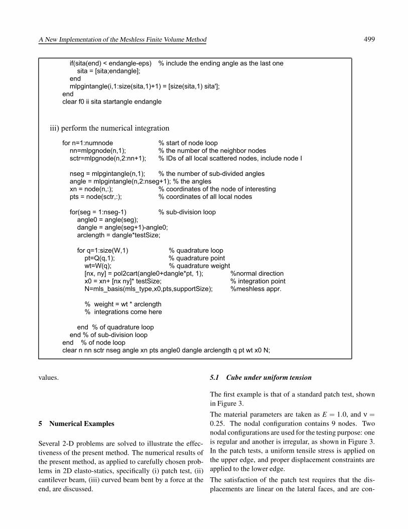
if(sita(end) < endangle-eps) % include the ending angle as the last one sita = [sita;endangle]; end mlpgintangle(i,1:size(sita,1)+1) = [size(sita,1) sita']; endclear f0 ii sita startangle endangle
iii) perform the numerical integration
for n=1:numnode % start of node loop nn=mlpgnode(n,1); % the number of the neighbor nodes sctr=mlpgnode(n,2:nn+1); % IDs of all local scattered nodes, include node I
nseg = mlpgintangle(n,1); % the number of sub-divided angles angle = mlpgintangle(n,2:nseg+1); % the angles xn = node(n,:); % coordinates of the node of interesting pts = node(sctr,:); % coordinates of all local nodes
for(seg = 1:nseg-1) % sub-division loop angle0 = angle(seg); dangle = angle(seg+1)-angle0; arclength = dangle*testSize; for q=1:size(W,1) % quadrature loop pt=Q(q,1); % quadrature point wt=W(q); % quadrature weight [nx, ny] = pol2cart(angle0+dangle*pt, 1); %normal direction x0 = xn+ [nx ny]* testSize; % integration point N=mls_basis(mls_type,x0,pts,supportSize); %meshless appr. % weight = wt * arclength % integrations come here
end % of quadrature loop end % of sub-division loop end % of node loop clear n nn sctr nseg angle xn pts angle0 dangle arclength q pt wt x0 N;
values.
5 Numerical Examples
Several 2-D problems are solved to illustrate the effec-tiveness of the present method. The numerical results ofthe present method, as applied to carefully chosen prob-lems in 2D elasto-statics, specifically (i) patch test, (ii)cantilever beam, (iii) curved beam bent by a force at theend, are discussed.
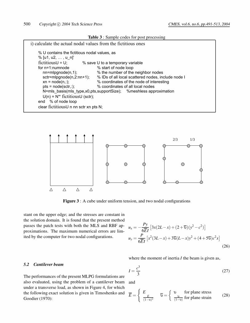
5.1 Cube under uniform tension
The first example is that of a standard patch test, shownin Figure 3.
The material parameters are taken as E = 1.0, and ν =0.25. The nodal configuration contains 9 nodes. Twonodal configurations are used for the testing purpose: oneis regular and another is irregular, as shown in Figure 3.In the patch tests, a uniform tensile stress is applied onthe upper edge, and proper displacement constraints areapplied to the lower edge.
The satisfaction of the patch test requires that the dis-placements are linear on the lateral faces, and are con-
500 Copyright c© 2004 Tech Science Press CMES, vol.6, no.6, pp.491-513, 2004
Table 3 : Sample codes for post processing
i) calculate the actual nodal values from the fictitious ones
% U contains the fictitious nodal values, as % [u1, u2, … , u_n]’
fictitiousU = U; % save U to a temporary variable
for n=1:numnode % start of node loop nn=mlpgnode(n,1); % the number of the neighbor nodes sctr=mlpgnode(n,2:nn+1); % IDs of all local scattered nodes, include node I xn = node(n,:); % coordinates of the node of interesting pts = node(sctr,:); % coordinates of all local nodes N=mls_basis(mls_type,x0,pts,supportSize); %meshless approximation
U(n) = N'* fictitiousU (sctr);
end % of node loop
clear fictitiousU n nn sctr xn pts N;
2/3 1/3
Figure 3 : A cube under uniform tension, and two nodal configurations
stant on the upper edge; and the stresses are constant inthe solution domain. It is found that the present methodpasses the patch tests with both the MLS and RBF ap-proximations. The maximum numerical errors are lim-ited by the computer for two nodal configurations.
5.2 Cantilever beam
The performances of the present MLPG formulations arealso evaluated, using the problem of a cantilever beamunder a transverse load, as shown in Figure 4, for whichthe following exact solution is given in Timoshenko andGoodier (1970):
ux = − Py
6EI
[3x(2L−x)+(2+υ)(y2 −c2)
]uy =
P
6EI
[x2(3L−x)+3υ(L−x)y2 +(4+5υ)c2x
](26)
where the moment of inertia I the beam is given as,
I =c3
3(27)
and
E =
E
E(1−υ)2
υ =
υ for plane stressυ
(1−υ) for plane strain (28)

A New Implementation of the Meshless Finite Volume Method 501
P
L
2c x
y
Figure 4 : A cantilever beam under an end load
P
P
P
(c) 441 nodes ( =0.5)d
(b) 125 nodes ( =1.0)d
(a) 39 nodes ( =2.0)d
Figure 5 : three nodal configurations for a cantilever beam
The corresponding stresses are
σx = −PI(L−x)y
σy = 0
σxy = − P2I
(y2 −c2) (29)
The problem is solved for the plane stress case with P =1, E = 1, c = 2, L = 24 and υ = 0.25. Regular uniformnodal configurations with nodal distances, d, of 2.0, 1.0,
and 0.5 are used, as shown in Figure 5. The numbers ofnodes are 39, 125, and 441, respectively.
First, the problem is solved by using the MLS approx-imation, with a support size of 1.15d and a test size of0.6d. The vertical displacements are shown in Figure6a, b, and c, for the three nodal configurations, respec-tively. They agree with the analytical solution very well.The relative error of the maximum displacement is 0.8%even when a very coarse nodal configuration with only

502 Copyright c© 2004 Tech Science Press CMES, vol.6, no.6, pp.491-513, 2004
0 0.1 0.2 0.3 0.4 0.5 0.6 0.7 0.8 0.9 10
0.2
0.4
0.6
0.8
1
x/L
Nor
mal
ized
Ver
tical
Dis
plac
emen
t
AnalyticalMLPG FVM (MLS)
Figure 6a : Normalized vertical displacement of a cantilever beam under an end loading(39 nodes with nodal distance d = 2.0)
0 0.1 0.2 0.3 0.4 0.5 0.6 0.7 0.8 0.9 10
0.2
0.4
0.6
0.8
1
1.2
x/L
Nor
mal
ized
Ver
tical
Dis
plac
emen
t
AnalyticalMLPG FVM (MLS)
Figure 6b : Normalized vertical displacement of a cantilever beam under an end loading(125 nodes with nodal distance d = 1.0)

A New Implementation of the Meshless Finite Volume Method 503
0 0.1 0.2 0.3 0.4 0.5 0.6 0.7 0.8 0.9 10
0.2
0.4
0.6
0.8
1
x/L
Nor
mal
ized
Ver
tical
Dis
plac
emen
t
AnalyticalMLPG FVM (MLS)
Figure 6c : Normalized vertical displacement of a cantilever beam under an end loading(441 nodes with nodal distance d = 0.5)
39 nodes is used, as shown in Figure 6a.
The effects of the approximation methods, the supportsize, and the test-domain size are studied for the presentmethod (MLPG FVM). The approximations are the MLSwith the first order polynomials (labeled as MLS1), theMLS with second order polynomials (labeled as MLS2),and the RBF augmented with the first order polynomi-als (labeled as RBF), respectively. The support size andthe test size are related to the nodal distance, d. Nor-mally, the ratio of the support size is greater than 1.0. Itshould be greater than 2.0 for the MLS2, to make surethat there are enough points to support the nodes on theglobal boundary. The ratio of the test-domain size is cho-sen to be less than 1.0 in the present study. They are de-tailed in the following sub-sections.
5.2.1 Effects of the test-domain size
The local sub-domain is one of the key concepts for theMLPG approach. As over-lapping sub-domains are used,the test-domain size (or the size of the sub-domain) af-fects the accuracy of the solution and the efficiency of themethod. It is very different from the non-over-lappingmethods, in which the background cells are required to
partition the solution domain. In the present study, thetest-domain size is chosen to be proportional to the nodaldistance, d. Theoretically, the ratio is very flexible. Inpractice, it is chosen to be less than 1.0 to ensure thatthe local sub-domains of the internal nodes are entirelywithin the solution domain, without being intersected bythe global boundary. It is chosen to be greater than 0.5 toensure the sub-domains are over-lapping. In the presentstudy, four ratios are used as 0.5, 0.6, 0.7 and 0.8. Thesupport size is fixed as 1.15d for the MLS1 and the RBF,and 2.5d for the MLS2.
As all methods give the reasonable results, the relative er-rors of the maximum displacements are used to examinethe effects of the test-domain size. Three nodal config-urations are used to examine the displacement errors, asshown Figure 7a,b, and c, respectively.
The MLS1 gives the most accurate results among thethree approximations. The maximum error is 0.8% evenonly 39 nodes are used. It can be seen that good accu-racy is obtained when the test-domain size is 0.6d. It isnoticeable that the accuracy is less sensitive to the test-domain size from 0.5 ∼ 0.7d, as the sub-domains areslightly over-lapping. However, the RBF approximation

504 Copyright c© 2004 Tech Science Press CMES, vol.6, no.6, pp.491-513, 2004
0.001
0.01
0.1
1
0.5 0.6 0.7 0.8
Normalized radius of test domain (r/d)
Rela
tive
disp
lace
men
t err
or
MLPG FVM (MLS 1)
MLPG FVM (MLS 2)MLPG FVM (RBF)
Figure 7a : Influence of the test-domain size in a cantilever beam under an end load(39 nodes with nodal distance d = 2.0)
0.001
0.01
0.1
1
0.5 0.6 0.7 0.8
Normalized radius of test domain (r/d)
Rel
ativ
e di
spla
cem
ent e
rror
MLPG FVM (MLS 1)
MLPG FVM (MLS 2)MLPG FVM (RBF)
Figure 7b : Influence of the test-domain size in a cantilever beam under an end load(125 nodes with nodal distance d = 1.0)

A New Implementation of the Meshless Finite Volume Method 505
0.0001
0.001
0.01
0.1
0.5 0.6 0.7 0.8
Normalized radius of test domain (r/d)
Rel
ativ
e di
spla
cem
ent e
rror
MLPG FVM (MLS 1)MLPG FVM (MLS 2)
MLPG FVM (RBF)
Figure 7c : Influence of the test-domain size in a cantilever beam under an end load(441 nodes with nodal distance d =0.5)
becomes more stable when a larger test-domain size isused. It may be due to the non-continuous shape func-tion.
5.2.2 Effects of the support size
The support size (or the size of the influence domain) is avery important in meshless methods. It is related to boththe accuracy of the solution, as well as the computationalefficiency. For a smaller size, the meshless approxima-tion algorithms may be singular and the shape functioncan not be constructed because of too few nodes. Thesupport size is also chosen to be proportional to the nodaldistance. In the present study, four ratios are used for theMLS1 and the RBF, as 1.15, 1.25, 1.5, and 1.8, and threefor the MLS2 are 2.05, 2.5 and 2.8. The test size is cho-sen as 0.6d.
The relative errors of the maximum displacements areshown in Figure 8.
Again, the MLS1 gives the most accurate results amongthe three approximations. In addition, the results are lesssensitive to the support size when the MLS1 is used witha smaller support size. It makes the present method veryefficient by speeding up the MLS approximation. The
MLS2 is also less sensitive to the support size. However,the RBF gives better results when the suitable supportsize is used.
5.2.3 Convergence rate
The convergence rate is studied with three nodal config-urations. The test-domain size is chosen to be 0.6d, andthe support size is 1.15d for the MLS1 and RBF and 2.5dfor the MLS2. The relative errors of the maximum dis-placement are used for showing the convergence rate inFigure 9.
The results clearly show that a stable convergence rateis obtained for the present MLPG finite volume methodwith all three approximations.
5.3 Curved beam
As the last example, the problem of a curved beam un-der an end load is used to evaluate the present method.The problem is shown in Figure 10, for which the fol-lowing exact solution is given in Timoshenko and Good-

506 Copyright c© 2004 Tech Science Press CMES, vol.6, no.6, pp.491-513, 2004
0.001
0.01
0.1
1
1 1.5 2 2.5 3
Normalized radius of support domain (r/d)
Rel
ativ
e di
spla
cem
ent e
rror
MLPG FVM (MLS 1)MLPG FVM (MLS 2)MLPG FVM (RBF)
Figure 8a : Influence of the support size in a cantilever beam under an end load(39 nodes with nodal distance d = 2.0)
0.0001
0.001
0.01
0.1
1
1 1.5 2 2.5 3
Normalized radius of support domain (r/d)
Rel
ativ
e di
spla
cem
ent e
rror
MLPG FVM (MLS 1)MLPG FVM (MLS 2)MLPG FVM (RBF)
Figure 8b : Influence of the support size in a cantilever beam under an end load(125 nodes with nodal distance d = 1.0)
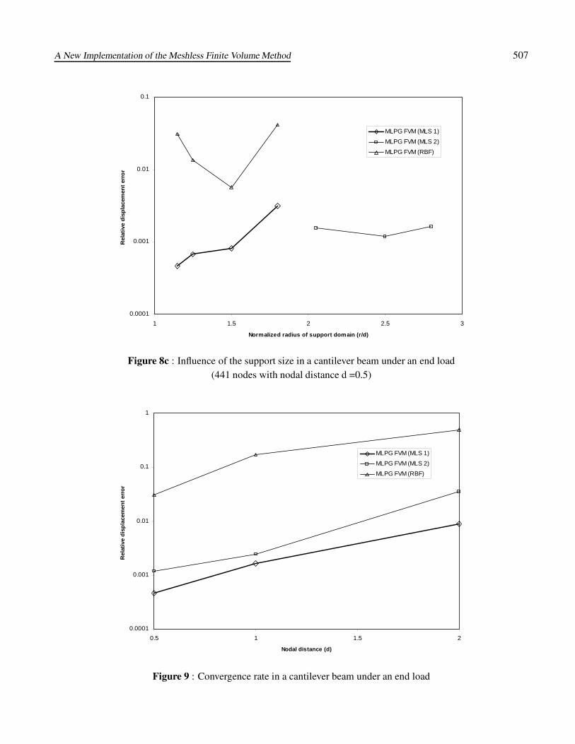
A New Implementation of the Meshless Finite Volume Method 507
0.0001
0.001
0.01
0.1
1 1.5 2 2.5 3
Normalized radius of support domain (r/d)
Rel
ativ
e di
spla
cem
ent e
rror
MLPG FVM (MLS 1)MLPG FVM (MLS 2)MLPG FVM (RBF)
Figure 8c : Influence of the support size in a cantilever beam under an end load(441 nodes with nodal distance d =0.5)
0.0001
0.001
0.01
0.1
1
0.5 1 1.5 2
Nodal distance (d)
Rel
ativ
e di
spla
cem
ent e
rror
MLPG FVM (MLS 1)
MLPG FVM (MLS 2)MLPG FVM (RBF)
Figure 9 : Convergence rate in a cantilever beam under an end load

508 Copyright c© 2004 Tech Science Press CMES, vol.6, no.6, pp.491-513, 2004
P
a
y
b
xθ
r
Figure 10 : A curved bar with an end load
ier (1970):
ur =P
E[−2Dθcosθ+ sinθ(D(1−υ) logr
+A(1−3υ)r2 +B(1+υ)
r2 )
+K sinθ+Lcos θ]
uθ =P
E[2Dθ sinθ−cos θ(−D(1−υ) logr
+A(5+υ)r2 +B(1+υ)
r2 )
+D(1+υ)cosθ+K cosθ+Lsinθ] (30)
where the constants are given as,
N = a2 −b2 +(a2 +b2) logba
A =1
2NB = −a2b2
2N
D = −a2 +b2
NL = Dπ
K = −(D(1−υ) logr0 +A(1−3υ)r20 +
B(1+υ)r2
0
)
r0 =a+b
2(31)
The corresponding stresses are
σr = P(2Ar− 2Br3 +
Dr
) sinθ
σθ = P(6Ar +2Br3 +
Dr) sinθ
σrθ = −P(2Ar− 2Br3 +
Dr)cosθ
(32)
The problem is solved for the plane stress case with P =1, E = 1, a = 13, b = 17 and υ = 0.25. Regular uniformnodal configurations with nodal distances, d, of 2.0, 1.0,and 0.5 are used, as shown in Figure 11. The numbers ofnodes are 39, 125, and 441, respectively.
The displacement and stress fields are more complicatedthan those in the case of a straight beam, with many non-polynomial terms. However, the first order MLS approx-imation is still used to solve this problem, with a supportsize of 1.25d and a test-domain size of 0.6d. The hor-izontal and vertical displacements are shown in Figure12a, b, and c, for the three nodal configurations, respec-tively. They agree with the analytical solution very well.
The relative errors of the maximum displacements areless than 2% even when only 39 nodes are used, as shownin Figure 12a, and they are reduced to less than 0.08%when 441 nodes are used. The influence of the test do-main size is also studied in this problem, as shown inFigure 13.
Again, it confirms that the MLS approximation is not

A New Implementation of the Meshless Finite Volume Method 509
P
P
P
(c) 441 nodes ( =0.5)d
(b) 125 nodes ( =1.0)d
(a) 39 nodes ( =2.0)d
Figure 11 : three nodal configurations for a curved cantilever beam
sensitive to the test-domain size when the local sub-domains are slightly over-lapped. The present methodalso gives a fast convergence rate by using three nodalconfigurations, as shown Figure 14.
6 Closure
A new Meshless Finite Volume Method (MFVM) is de-veloped through a new MLPG ”Mixed” approach. Thedifferentiation of the shape function is eliminated, byinterpolating the strains directly, as independent vari-ables in the local weak form. It reduces the continuity-requirement on the trial function by one-order, and asmaller support size can be used in the meshless approx-
imations with a lower-order polynomial basis. The com-putational efficiency is improved, due to these two keyaspects in the newly developed meshless method. Thenumerical results demonstrate the accuracy of the presentmethods for problems whose analytical solutions con-tain both polynomial and non-polynomial basis. Con-vergence studies in the numerical examples show thatthe present method possesses an excellent rate of con-vergence.
Acknowledgement: This work was supported by theArmy Research Laboratory, and the ARO, under the cog-nizance of Drs. R. Namburu, and B. LaMattina. The firsttwo authors gratefully acknowledge this support.

510 Copyright c© 2004 Tech Science Press CMES, vol.6, no.6, pp.491-513, 2004
0 15 30 45 60 75 900
0.2
0.4
0.6
0.8
1
Thita
Nor
mal
ized
Dis
plac
emen
ts
Ux AnalyticalMLPG FVM (MLS1)Uy AnalyticalMLPG FVM (MLS1)
Figure 12a : Normalized displacements of a curved cantilever beam under an end loading(39 nodes with nodal distance d = 2.0)
0 15 30 45 60 75 900
0.2
0.4
0.6
0.8
1
Thita
Nor
mal
ized
Dis
plac
emen
ts
Ux AnalyticalMLPG FVM (MLS1)Uy AnalyticalMLPG FVM (MLS1)
Figure 12b : Normalized displacements of a curved cantilever beam under an end loading(125 nodes with nodal distance d = 1.0)

A New Implementation of the Meshless Finite Volume Method 511
0 15 30 45 60 75 900
0.2
0.4
0.6
0.8
1
Thita
Nor
mal
ized
Dis
plac
emen
ts
Ux AnalyticalMLPG FVM (MLS1)Uy AnalyticalMLPG FVM (MLS1)
Figure 12c : Normalized displacements of a curved cantilever beam under an end loading(441 nodes with nodal distance d = 0.5)
0.0001
0.001
0.01
0.1
1
0.5 0.6 0.7 0.8
Normalized radius of test domain (r/d)
Rel
ativ
e D
ispl
acem
ent E
rror
s
MLPG FVM (MLS 1, d=2.0) Ux Uy
MLPG FVM (MLS 1, d=1.0) Ux Uy
MLPG FVM (MLS 1, d=0.5) Ux Uy
Figure 13 : Influence of the test-domain size in a curved cantilever beam under an end load

512 Copyright c© 2004 Tech Science Press CMES, vol.6, no.6, pp.491-513, 2004
0.0001
0.001
0.01
0.1
1
0.5 0.6 0.7 0.8
Normalized radius of test domain (r/d)
Rel
ativ
e D
ispl
acem
ent E
rror
sMLPG FVM (MLS 1, d=2.0) Ux Uy
MLPG FVM (MLS 1, d=1.0) Ux Uy
MLPG FVM (MLS 1, d=0.5) Ux Uy
Figure 14 : Convergence rate in a curved cantilever beam under an end load
References
Atluri, S. N. (2004): The Meshless Local Petrov-Galerkin ( MLPG) Method for Domain & Boundary Dis-cretizations, Tech Science Press, 680 pages.
Atluri, S. N.; Han, Z. D.; Shen, S. (2003): MeshlessLocal Patrov-Galerkin (MLPG) approaches for weakly-singular traction & displacement boundary integral equa-tions, CMES: Computer Modeling in Engineering & Sci-ences, vol. 4, no. 5, pp. 507-517.
Atluri, S. N.; Kim, H. G.; Cho, J. Y. (1999): A CriticalAssessment of the Truly Meshless Local Petrov Galerkin(MLPG) and Local Boundary Integral Equation (LBIE)Methods, Computational Mechanics, 24:(5), pp. 348-372.
Atluri, S. N.; Shen, S. (2002): The meshless localPetrov-Galerkin (MLPG) method: A simple & less-costly alternative to the finite element and boundary ele-ment methods. CMES: Computer Modeling in Engineer-ing & Sciences, vol. 3, no. 1, pp. 11-52
Atluri, S. N.; Zhu, T. (1998): A new meshless localPetrov-Galerkin (MLPG) approach in computational me-
chanics. Computational Mechanics., Vol. 22, pp. 117-127.
Dilts, G. A. (1999): Moving-Least-Squares-Particle Hy-drodynamics - I. Consistency and Stability, InternationalJournal for Numerical Methods in Engineering, vol. 44,pp. 1115-1155.
Gingold, R. A.; Monaghan, J. J. (1977): Smoothedparticle hydrodynamics, theory and application to non-spherical stars, Mon. Not. Roy. Astr. Soc., vol. 181, pp.375-389.
Golberg, M. A.; Chen, C. S.; Bowman, H. (1999):Some recent results and proposals for the use of radialbasis functions in the BEM, Engineering Analysis withBoundary Elements, vol. 23, pp. 285-296.
Han. Z. D.; Atluri, S. N. (2003a): On Simple For-mulations of Weakly-Singular Traction & DisplacementBIE, and Their Solutions through Petrov-Galerkin Ap-proaches, CMES: Computer Modeling in Engineering &Sciences, vol. 4 no. 1, pp. 5-20.
Han. Z. D.; Atluri, S. N. (2003b): Truly Meshless LocalPetrov-Galerkin (MLPG) Solutions of Traction & Dis-
A New Implementation of the Meshless Finite Volume Method 513
placement BIEs, CMES: Computer Modeling in Engi-neering & Sciences, vol. 4 no. 6, pp. 665-678.
Han. Z. D.; Atluri, S. N. (2004a): Meshless Lo-cal Petrov-Galerkin (MLPG) approaches for solving 3DProblems in elasto-statics, CMES: Computer Modelingin Engineering & Sciences, vol. 6 no. 2, pp. 169-188.
Han. Z. D.; Atluri, S. N. (2004b): A Meshless LocalPetrov-Galerkin (MLPG) Approach for 3-DimensionalElasto-dynamics, CMC: Computers, Materials & Con-tinua, vol. 1 no. 2, pp. 129-140.
Johnson, G. R.; Beissel, S. R. (1996): Normalizedsmoothing functions for SPH impact computations, In-ternational Journal for Numerical Methods in Engineer-ing, vol. 39, pp. 2725-2741.
Johnson, G.R.; Stryk, R. A.; Beissel, S.R.; Holmquist,T.J. (2002): An algorithm to automatically convert dis-torted finite elements into meshless particles during dy-namic deformation. Int. J. Impact Eng., vol. 27, pp.997-1013.
Li, Q.; Shen, S.; Han, Z. D.; Atluri, S. N. (2003):Application of Meshless Local Petrov-Galerkin (MLPG)to Problems with Singularities, and Material Discontinu-ities, in 3-D Elasticity, CMES: Computer Modeling inEngineering & Sciences, vol. 4 no. 5, pp. 567-581.
Lin, H.; Atluri, S. N. (2001): The Meshless LocalPetrov-Galerkin (MLPG) Method for Solving Incom-pressible Navier-Stokes Equations CMES: ComputerModeling in Engineering & Sciences, vol. 2, no. 2, pp.117-142.
Lucy (1977): A numerical approach to the testing of ses-sion hypothesis, Astronomical Journal, vol. 82, pp. 1013–1024.
Sellountos, E. J.; Polyzos, D. (2003): A MLPG (LBIE)method for solving frequency domain elastic problems,CMES: Computer Modeling in Engineering & Sciences,vol. 4, no. 6, pp. 619-636
Timoshenko, S. P.; Goodier, J. N. (1976): Theory ofElasticity, 3rd edition, McGraw Hill.


![Prediction of Groundwater Fluctuations Using Meshless ...nmce.kntu.ac.ir/article-1-216-en.pdfanalyze groundwater flow [5]. Mostly, the finite difference method and the finite element](https://static.fdocuments.net/doc/165x107/60ae0f5c9525d23ed35b5a68/prediction-of-groundwater-fluctuations-using-meshless-nmcekntuacirarticle-1-216-enpdf.jpg)