a new gis-based spatial modelling approach for desertification risk assessment in the
231
DIPARTIMENTO DI SCIENZE DELL’AMBIENTE FORESTALE E DELLE SUE RISORSE CORSO DI DOTTORATO DI RICERCA IN ECOLOGIA FORESTALE – XX CICLO A NEW GIS-BASED SPATIAL MODELLING APPROACH FOR DESERTIFICATION RISK ASSESSMENT IN THE MEDITERRANEAN AREA. AN ITALIAN CASE STUDY: SARDINIA ISLAND Settore Scientifico Disciplinare – AGR/05 Dottorando: Monia Santini Coordinatore: Prof. Paolo De Angelis Tutori: Co-Tutore: Prof. Riccardo Valentini Dr.ssa Paola Molinari Dr. Paolo Ciccioli
Transcript of a new gis-based spatial modelling approach for desertification risk assessment in the
DIPARTIMENTO DI SCIENZE DELL’AMBIENTE FORESTALE E DELLE SUE RISORSE
CORSO DI DOTTORATO DI RICERCA IN ECOLOGIA FORESTALE – XX CICLO
A NEW GIS-BASED SPATIAL MODELLING APPROACH FOR DESERTIFICATION RISK
ASSESSMENT IN THE MEDITERRANEAN AREA. AN ITALIAN CASE STUDY: SARDINIA ISLAND
Settore Scientifico Disciplinare – AGR/05
Dottorando: Monia Santini Coordinatore: Prof. Paolo De Angelis Tutori: Co-Tutore: Prof. Riccardo Valentini Dr.ssa Paola Molinari Dr. Paolo Ciccioli

INTRODUCTION 1 1. THE DESERTIFICATION ISSUE 5
1.1. INTRODUCTION 5 1.2. DEFINITIONS OF DESERTIFICATION 6
1.2.1. Land Degradation 6 1.2.2. Causes 7
1.2.2.1. Climate 9 1.2.2.2. Human activities 10
1.2.3. Manifestations and Effects 10 1.2.4. Reversibility 11 1.2.5. Threatened areas 11
1.3. ACTIONS AGAINST DESERTIFICATION 15 1.3.1. World action 15 1.3.2. European Actions 15 1.3.3. Italian Actions 16
1.4. DESERTIFICATION AS A RESEARCH ISSUE 16 1.4.1. First approaches 16 1.4.2. The indicators 18 1.4.3. D.P.S.I.R. framework 19 1.4.4. Projects regarding desertification 20
2. DESERTIFICATION IN THE STUDY AREA AND NEW APPROACH 28
2.1. INTRODUCTION 28 2.2. THE STUDY AREA: ISLAND OF SARDINIA 28
2.2.1. General description of the area 28 2.2.2. The desertification phenomenon in Sardinia 30
2.2.2.1. Agriculture 32 2.2.2.2. Pastoral activities 32 2.2.2.3. Urbanisation 33 2.2.2.4. Quarrying and mining activities 34 2.2.2.5. Water resources contamination 35 2.2.2.6. Fires 35 2.2.2.7. Soil erosion 35 2.2.2.8. Decline in organic matter 36
2.2.3. Previous regional experiences: state of the art 36 2.3. THE NEW PROPOSED METHODOLOGY 41
2.3.1. Vulnerability and risk 42 2.3.2. Why models? 42 2.3.3. Why GIS? 43 2.3.4. The methodology 43 2.3.5. Spatial and Temporal scale 45 2.3.6. Models 45 2.3.7. Relative importance of the degradation processes 46 2.3.8. The Integrated Desertification Index (IDI) 46
2.4. TOOLS AND SOFTWARE 48 3. THE WATER EROSION ASSESSMENT MODEL - RUSLE 50
3.1. INTRODUCTION 50 3.2. DESCRIPTION OF THE MODEL 50 3.3. PARAMETERIZATION AND MODIFICATIONS TO THE MODEL 51
3.3.1. R factor: rain erosivity 51 3.3.2. K factor: soil erodibility 52 3.3.3. LS factor: topography 54 3.3.4. C factor: vegetation cover 56 3.3.5. P factor: management practices against erosion 57

3.4. PRODUCTION AND FORMAT OF INPUT DATA 57 3.4.1. Erodible areas 58 3.4.2. R factor 59 3.4.3. K factor 60 3.4.4. LS factor 62 3.4.5. P factor 63 3.4.6. C factor 64 3.4.7. Other input data 65
3.5. SIMULATION AND RESULT DISCUSSION 66 4. THE OVERGRAZING ASSESSMENT MODEL - CAIA 71
4.1. INTRODUCTION 71 4.2. DESCRIPTION OF THE MODEL 71 4.3. PARAMETERIZATION AND MODIFICATIONS TO THE MODEL 73 4.4. PRODUCTION AND FORMAT OF INPUT DATA 76
4.4.1. Sustainable CAIA 76 4.4.2. Actual CAIA 76 4.4.3. Output structure 76
4.5. SIMULATION AND RESULT DISCUSSION 77 5. THE VEGETATION PRODUCTIVITY ASSESSMENT MODEL - MOD17 79
5.1. INTRODUCTION 79 5.2. DESCRIPTION OF THE MODEL 79
5.2.1. The GPP algorithm 80 5.2.2. Examples of validation of the model 81
5.3. PRODUCTION AND FORMAT OF INPUT DATA 83 5.3.1. Radiation use efficiency, Tmin_scalar and VPD_scalar 84 5.3.2. Climatic Data 85
5.4. GIS-BASED TOOL 85 5.5. SIMULATION AND RESULT DISCUSSION 86
6. THE SOIL PRODUCTIVITY ASSESSMENT MODEL - CENTURY 90
6.1. INTRODUCTION 90 6.2. DESCRIPTION OF THE MODEL 90
6.2.1. Examples of validation of the model 91 6.3. PRODUCTION AND FORMAT OF INPUT DATA 94
6.3.1. Textural data 97 6.3.2. Field capacity and wilting point 97 6.3.3. Density 97 6.3.4. Soil Organic Carbon (SOC) 97 6.3.5. Climatic data 98 6.3.6. C and N of litter, roots, stems and leaves 98 6.3.7. Final database 98 6.3.8. “.100” file creation 99 6.3.9. Output structure 100
6.4. SIMULATION AND RESULT DISCUSSION 100 7. THE WIND EROSION ASSESSMENT MODEL - WEAM 104
7.1. INTRODUCTION 104 7.2. DESCRIPTION OF THE MODEL 105
7.2.1. Threshold wind friction velocity 105 7.2.2. Horizontal and vertical fluxes 107 7.2.3. Examples of validation of the model 107
7.3. PARAMETERIZATION AND MODIFICATIONS TO THE MODEL 110 7.3.1. Particle Size Distribution 110 7.3.2. Wind friction velocity 112

7.3.2.1. Soil moisture factor 112 7.3.2.2. Roughness factor 113
7.4. WEAM SIMULATION TOOL 113 7.5. PRODUCTION AND FORMAT OF INPUT DATA 114
7.5.1. Erodible areas 114 7.5.2. Soil roughness 114 7.5.3. Textural composition 115 7.5.4. Vegetation/soil drag coefficient 115 7.5.5. Daily climatic data 116 7.5.6. Leaf Area Index (LAI) 116 7.5.7. Other input data 118
7.6. SIMULATION AND RESULT DISCUSSION 118 8. THE SEAWATER INTRUSION ASSESSMENT MODEL - SHARP 120
8.1. INTRODUCTION 120 8.1.1. The physical process 121
8.2. DESCRIPTION OF THE MODEL 123 8.2.1. Boundary terms 124 8.2.2. Leakage terms 124 8.2.3. Sources and sinks 125
8.3. PARAMETERIZATION, MODIFICATIONS TO THE MODEL AND CRITICALITY 126 8.3.1. Criticality of the data availability in Sardinia 126
8.4. PREPARATION AND FORMAT OF INPUT DATA 127 8.4.1. Non spatialized input data 129 8.4.2. Spatialized input data 129
8.4.2.1. Aquifer data 129 8.4.2.2. Well data 131
8.5. SIMULATION AND RESULT DISCUSSION 132 9. ANALYSIS OF IDI RESULTS 135
9.1. INTRODUCTION 135 9.2. IDI APPLICATION 135
9.2.1. Standardization of model results 135 9.2.1.1. Normalization of erosion model results 136 9.2.1.2. Normalization of productivity model results 141
9.2.2. Weighting the indices 144 9.3. IDI RESULTS 146
9.3.1. Extraction of hotspots 148 9.3.2. Comparison of IDI with a simplified-IDI 149 9.3.3. Field verification 150 9.3.4. Geographic characteristic influence over IDI 154 9.3.5. Risk evaluation on a basin scale 155 9.3.6. Risk evaluation on a municipality scale 156 9.3.7. Risk evaluation on a land use scale 158
10. METHODOLOGY APPLICATION AT LARGER SCALE: ”PARTIAL-IDI” 159
10.1. INTRODUCTION 159 10.2. TEST AREA: RIO MANNU 159 10.3. NEW INPUT PRODUCTION 161
10.3.1. Pedologic Map 161 10.3.2. Updating of the Land Use map 162 10.3.3. Precipitation data 162 10.3.4. Normalization Difference Vegetation Index 163 10.3.5. Digital Elevation Model (DEM) 163
10.4. APPLICATION OF THE MODELS TO TEST-AREA 163
10.4.1. RUSLE 163 10.4.2. WEAM 169 10.4.3. MOD17 170 10.4.4. CENTURY 171 10.4.5. CAIA 172
10.5. PARTIAL-IDI 173 11. FUTURE SCENARIOS OF DESERTIFICATION 176
11.1. INTRODUCTION 176 11.2. MODELLING OF LAND USE CHANGE 176
11.2.1. CLUE-s model 176 11.2.1.1. Main Principles 176 11.2.1.2. Driving factors 177 11.2.1.3. Model Description 177 11.2.1.4. Spatial Analysis 178 11.2.1.5. Decision rules 179 11.2.1.6. Allocation 180 11.2.1.7. Model limits 181
11.3. CLUE-S IMPLEMENTATION IN THE STUDY AREA 181 11.3.1. Driving factors 182 11.3.2. Land use 185 11.3.3. Statistical analysis 186 11.3.4. Land Use demand 187 11.3.5. Decision rules and elasticity 189 11.3.6. Convergence criteria 189 11.3.7. Restriction 190
11.4. SCENARIOS OF IDI 191 11.4.1. CENTURY 192 11.4.2. SHARP 192 11.4.3. RUSLE 192 11.4.4. WEAM 192 11.4.5. CAIA 192 11.4.6. IDI estimation 193
CONCLUSIONS 197 REFERENCES 199 ANNEX A 208 ANNEX B 218 ANNEX C 219 ANNEX D 221 ANNEX E 223
Introduction
1
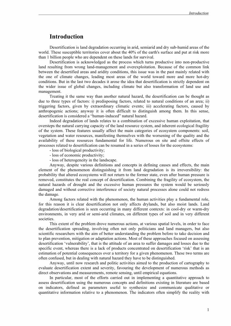
Introduction Desertification is land degradation occurring in arid, semiarid and dry sub-humid areas of the
world. These susceptible territories cover about the 40% of the earth's surface and put at risk more than 1 billion people who are dependent on these lands for survival.
Desertification is acknowledged as the process which turns productive into non-productive land resulting from wrong land-management and overexploitation. Because of the common link between the desertified areas and aridity conditions, this issue was in the past mainly related with the one of climate changes, leading most areas of the world toward more and more hot-dry conditions. But in the last two decades it arose the idea that desertification is strictly dependent on the wider issue of global changes, including climate but also transformation of land use and management.
Treating it the same way than another natural hazard, the desertification can be thought as due to three types of factors: i) predisposing factors, related to natural conditions of an area; ii) triggering factors, given by extraordinary climatic events; iii) accelerating factors, caused by anthropogenic actions; anyway it is often difficult to distinguish among them. In this sense, desertification is considered a “human-induced” natural hazard.
Indeed degradation of lands relates to a combination of excessive human exploitation, that oversteps the natural carrying capacity of the land resource system, and inherent ecological fragility of the system. These features usually affect the main categories of ecosystem components: soil, vegetation and water resources, manifesting themselves with the worsening of the quality and the availability of these resources fundamental for life. Numerous on site and offsite effects of processes related to desertification can be resumed in a series of losses for the ecosystems:
- loss of biological productivity; - loss of economic productivity; - loss of heterogeneity in the landscape. Anyway, despite various definitions and concepts in defining causes and effects, the main
element of the phenomenon distinguishing it from land degradation is its irreversibility: the probability that altered ecosystems will not return to the former state, even after human pressure is removed, constitutes the real concept of desertification. Combining the fragility of ecosystem, the natural hazards of drought and the excessive human pressures the system would be seriously damaged and without corrective interference of society natural processes alone could not redress the damage.
Among factors related with the phenomenon, the human activities play a fundamental role, for this reason it is clear desertification not only affects drylands, but also moist lands. Land degradation/desertification is seen occurring in many different contexts: in cool-dry or warm-dry environments, in very arid or semi-arid climates, on different types of soil and in very different societies.
This extent of the problem drove numerous actions, at various spatial levels, in order to face the desertification spreading, involving often not only politicians and land managers, but also scientific researchers with the aim of better understanding the problem before to take decision and to plan prevention, mitigation or adaptation actions. Most of these approaches focused on assessing desertification ‘vulnerability’, that is the attitude of an area to suffer damages and losses due to the specific event, whereas there is a lack of products concentrated on desertification ‘risk’ that is an estimation of potential consequences over a territory for a given phenomenon. These two terms are often confused, but in dealing with natural hazard they have to be distinguished.
Anyway, until now research and politic activities aimed to the production of cartography to evaluate desertification extent and severity, favouring the development of numerous methods as direct observations and measurements, remote sensing, until empirical equations.
In particular, most of the efforts carried out in implementing a quantitative approach to assess desertification using the numerous concepts and definitions existing in literature are based on indicators, defined as parameters useful to synthesize and communicate qualitative or quantitative information relative to a phenomenon. The indicators often simplify the reality with

Introduction
2
the aim of quantify complex processes sometimes difficult to measure or observe. Recently, the most useful indicators for assessing desertification are derived from the logic
model known as DPSIR (Driving force-Pressure-State-Impacts-Responses), developed by the Environmental European Agency. Anyway, these widely used indicators, also if combined together in order to give a more exhaustive assessment of desertification, show several limits. First of all they are static and too simple to represent the complexity of processes occurring on the land and their interactions with biota, and not able to represent with reliability the continuously changing world. Secondly, they are inadequate in their capability to provide future scenarios, which is one of the most urgent problem to address climate change signal and human pressures in future land degradation predictions.
For this reason the necessity of a new approach arose, an approach that is: i) capable to quantitatively estimate the risk of desertification, making an evaluation of the vulnerability relatively to the land use of a given territory, and ii) not only diagnostic but also prognostic, permitting to produce scenarios. This work had the purpose of developing a methodology for creating a plausible and feasible model to identify areas vulnerable and at risk of desertification.
In particular this was made for desertification risk evaluation in Sardinia (Italy), aiming to assess desertification risk of this region that, since last decades, suffered from severe land degradation problems. In this context, the Autonomous Regional Government of Sardinia funded the project called “Design and implementation of a G.I.S. (Geographic Information System) to monitor the areas of Sardinia at risk of desertification, with the specific indication of the components of this risk, included their parameterization”* that started in February 2005 (coordinated by Agriconsulting S.p.A. and ESRI Italia), and whose framework and implementation are the topic of this thesis.
The region of Sardinia is situated at the centre of western Mediterranean Sea; the Island is characterized by a high variability of landscapes due to their geologic, morphologic, pedologic and vegetation characteristics.
The study area, sharing many environmental characteristics with the other Mediterranean regions, shows a menacing interaction of soil erosion and overgrazing that affects the territory: the areas for breeding are often obtained through fires or ploughing to seed pasture on every kind of slope, making the soil more instable and susceptible to erosion, because of the removing of vegetation cover and the compaction of the soil, both increasing runoff processes. Among secondary factors of desertification in Sardinia there are the drought periods, the overexploitation of groundwater and consequent salinization, the high frequency and extension of firewood, the reduction of vegetation cover and the agricultural land abandonment.
We developed a new framework to assess desertification and land degradation based on a suite of models (in contrast with indicators) which are integrated in a Geographical Information Systems (GIS) environment and simulate a set of processes related to land degradation in the study area. We chose to couple GIS and models with the advantage of allowing environmental managers and scientists both to generate different scenarios simulating particular conditions and decisions both to display the outcomes in a spatial context, this functional for comparisons more easily than with tables, graphs or texts. But we differentiated our approach from the one of previous works, not only using models instead of indicators, but also distinguish the concept of vulnerability (i.e. the tendency if the territory to suffer from damages by desertification) from the one of risk (i.e. the gravity of the resulting damages according to the type of land exploitation).
This approach has the advantage to be dynamic and fully interacting with environmental and human variables, providing the possibility to derive future scenarios about desertification.
In particular our objectives were: 1) to assess the nature, the intensity and the relative influence of desertification factors; 2) to identify the direct and indirect impacts of desertification;
* “Progettazione e realizzazione di un Sistema Informativo Geografico per il monitoraggio delle aree della Sardegna a rischio di desertificazione, con la specifica indicazione delle componenti di tale rischio, compresa la parametrazione delle stesse”, bando G.U.C.E. serie n. S248-221050 del 24.12.2003

Introduction
3
3) to develop an evaluation procedure for desertification risk assessment; 4) to detect the most critical areas (Hotspots); 5) to promote software applications as decision support tool; 6) to favour the diffusion and the exchange of information. This thesis wants to present the rationale of the research, the methodological approach and
the application and validation experience. A large multi-thematic dataset was acquired, processed and re-arranged in a GIS
environment in order to model six degradation processes frequent in the study area: overgrazing, soil erosion (by wind and water), vegetation degradation, soil degradation and seawater intrusion. When necessary, the maps of model results were normalized to adimensional indices varying from 0 (representing no degradation) to 1 (representing irreversible degradation). These procedures were applied for two different periods: the early nineties and the present. Resulting degradation indices were then integrated into a final one, combining different aspects of desertification processes: their magnitude and their development rate, weighting them according to their significance and to the quality of their input data. The final Integrated Desertification Index (IDI) was classified into five levels of increasing severity and the results where verified by means of field survey in sites resulting as areas at risk.
The thesis is organized as follow. In the first part (Chapter 1) we illustrate the issue of desertification, its occurring and facing at various spatial levels until focusing on the study area (Chapter 2) and its criticalities, also describing actions already carried out in assessing desertification vulnerability, producing several cartographic products, then we introduce the new developed evaluation methodology. In the second part (Chapters from 3 to 8) we describe the degradation models used in the procedures, the modification made on them, their parameterization and their results for the two periods of reference. Afterward, in the third part we discuss the results of the application of the new GIS-modelling based methods for the study area (Chapter 9), the experience of application of the same methodology on a test areas resulted at risk from the first application in order to evaluate the performance of the methodology on a larger scale (Chapter 10), and the experiment of application of the method to simulate desertification scenarios for the future, deriving it by coupling of climate change and land use change predictions (Chapter 11). In the conclusions we resume the results of the research. The Annexes aid in more detailed description of used database (Annex A) and of several procedures for database treatment (Annexes from B to E).

PART I

Chapter 1 – The Desertification Issue
5
1. THE DESERTIFICATION ISSUE
1.1. Introduction The phenomenon known as desertification received extensive attention in last decades, since the time of the organization of the United Nations Conference On Desertification (UNCOD), hold in Nairobi in 1977, that was mainly a result of the impact of an extended drought in the West African Sahel in the early 1970s. That drought caused a loss of human lives and livestock and an invasive environmental deterioration. Although the role of the Sahelian drought in the increasing consideration of the desertification issue is commented in a lot of recent documents, papers and reports from many countries (e.g. Glantz, 1977; UN Secretariat, 1977), that drought was neither the first appearance of the desertification phenomenon nor the only reason for scientific interest in it (Glantz and Orlovsky, 1983). Indeed, despite the attention focused upon it in recent thirty years, desertification was not a new phenomenon: similar droughts occurred in 1911 and 1940, but the difference was that at the time of Sahelian episode television brought the images to the entire world. If we look at the historical occurrence during the last few centuries we can find three main epicentres of desertification: the Mediterranean region, the Mesopotamia and the Loessial Plateau of China. Particularly, what happened in the past two centuries is that the impact of human agricultural, industrial and extractive activities, when coupled with human induced climate variations, is leading to land degradation on an unprecedented extent. The Nairobi Conference in 1977 provided the biggest attention to the phenomenon (UN Secretariat, 1977). It described desertification as: "...the diminution or destruction of the biological potential of the land, which can lead ultimately to desert-like conditions…Desertification is a self-accelerating process, feeding on itself, and as it advances, rehabilitation costs rise exponentially. Action to combat desertification is required urgently before the costs of rehabilitation rise beyond practical possibility or before the opportunity to act is lost forever.” So desertification is a general land degradation problem, and the land degradation can happen in many different contexts: in cool-dry or warm-dry environments, in very arid or semi-arid climates, on different types of soil and in very different societies, both ancient and modern, both with advanced technologies and with traditional ones, both rich and poor, both capitalist and socialist and so on. As the desertification is such a complex phenomenon it requires the expertise of researchers in many different disciplines as climatology, soil science, meteorology, hydrology, range science, agronomy, veterinary medicine, as well as geography, political science, economy and anthropology. The concept has been defined in many different ways by researchers in those and other disciplines, as well as from many national and institutional perspectives, each highlighting different aspects of the phenomenon. In particular desertification is of great interest to climatologists in their efforts to understand climate variations and changes on both short and long terms. Indeed, with increasing pressure on governmental decision-makers for allowing populations to move into the climatically marginal areas, the implications of natural variations in climate became even more important in decisions relating to the use by society of its land in desertification-prone regions. One can easily assert that there will be always climatic deserts. However, man-induced extensions of these deserts or the creation of desert-like conditions in areas where they had never existed can and must be avoided. The climatologists both at national and international levels (e.g. World Meteorological Organization's Climate Programme and UNEP’s (United Nation Environment Program) World Climate Impacts Programme) have, in general, made the identification of the climatologic and meteorological aspects of desertification one of their most important priorities (Glantz and Orlovsky, 1983). In this chapter we will focus on the general concept of desertification phenomenon and on its aspects as: its relationships with land degradation, its causes, its effects, the different degrees of the phenomenon severity (reversibility or not) and the extent of the phenomenon. Then we will introduce briefly the actions undertaken at various scales (global, continental, national) together

Chapter 1 – The Desertification Issue
6
with some information about the most diffuse and used approaches (mainly in a research context) in dealing with desertification.
1.2. Definitions of desertification A review of the desertification literature shows a great confusion among definitions: there are numerous different descriptions of the process, giving the idea of the complexity of the phenomenon. This mix of meanings attributed to the concept leads to miscommunication among researchers, among policy-makers and, first of all, between researchers and policy-makers (Glantz and Orlovsky, 1983). Within the hundreds of existing definitions of desertification, many words are used to describe the phenomenon, some of which complement each other while others appear to be contradictory. The point on which they all agree, anyway, is that desertification is viewed as an adverse environmental process. The negative descriptors used in these definitions of desertification include: deterioration of ecosystems (e.g. Reining, 1978), degradation of various forms of vegetation (e.g. Le Houerou, 1975), destruction and diminution of biological potential (e.g. UNCOD, 1978), decay of a productive ecosystem (e.g. Hare, 1977), reduction of productivity (e.g. Kassas, 1977), decrease of biological productivity (e.g. Kovda, 1980), alteration in the biomass (e.g. UN Secretariat, 1977), intensification of desert conditions (e.g. WHO, 1980), impoverishment of ecosystems (e.g. Dregne, 1976) and so on. The first author defining desertification was Aubreville (1949) that looked at the phenomenon as a slow and underhand process but also as an event, which is the end state of a process of degradation. Each of used terms suggests changes from a favourable or preferred state (with respect to quality, societal value or ecological stability) to a less favoured one and each was used to describe the condition of vegetation, or moisture availability, or soil conditions, or atmospheric phenomena, depending on the particular definition. Other descriptors used in these definitions connote a movement or a transfer of the characteristics of a desert landscape into an area where such characteristics did not exist; these descriptors are: extension, encroachment, acceleration, spread, transformation etc. If one combines each of these negative and transfer descriptors with all the other factors cited in the existing definitions, desertification would include most kinds of environmental changes related to biological productivity. AGENDA 21, one of the most important documents of the United Nations Conference on Environment and Development (UNCED, 1992), describes desertification as “…land degradation in arid, semi-arid and dry sub-humid areas resulting from various factors, including climatic variations and human activities”. This definition is internationally accepted as the most complete one for describing the desertification phenomenon, being also the one officially considered by the UNCOD (1978). But finally Mainguet (1994), after a large review of the different definitions, concluded defining the process as: “the ultimate step of land degradation, the point when land becomes irreversibly sterile in human terms and with respect to reasonable economic limitation”. But this statement of the desertification perception needs to be further explained elaborating its five main concepts: (1) what is the “menace” (land degradation); 2) what are the “causes” (natural and anthropogenic); (3) what “effects” are produced by phenomenon; (4) the degree of “reversibility” of the phenomenon; (5) what are “the menaced territories” (drylands, but not only).
1.2.1. Land Degradation There are in general two main concepts in approaching desertification issue: - considering this as a loss of productivity of ecosystem caused by climatic condition changes and by human activities; - considering desertification as a long time, complex and intricate process involving, as precursor, the land degradation.

Chapter 1 – The Desertification Issue
7
Indeed, some researchers consider desertification to be a process of change, while others view it as the final result (an event) of several processes of change (land degradation). This distinction underlies one of the main disagreements about what constitutes desertification. Desertification-as-process has generally been viewed as a series of incremental (sometimes step-wise) changes in biological productivity in arid, semi-arid and sub-humid ecosystems. It can include such changes as a decline in yield of the same crop or, more drastically, a decrease in the density of the existing vegetative cover. Desertification-as-event is the creation of desert-like conditions (where perhaps none had existed in the recent past) as the end result of a process of changes (Glantz and Orlovsky, 1983). In both cases, the changes can be seen as prevailing only over the short term, with the degraded resource recovering quickly, or they may be the precursors of a strong deterioration process, causing a long-term and permanent alteration in the status of the resource. Land degradation therefore includes changes on soil quality, the reduction in available water, the diminution of vegetation resources and of biological diversity and the many other ways the overall integrity of land is menaced by inappropriate use. Despite this work will focus on the study of the desertification problem, nevertheless some parts of the study such as those concerning causes, processes and indicators will address both concepts: land degradation as fragmentary processes and desertification as the general phenomenon, since they are closely interrelated.
1.2.2. Causes There is a tendency to blame for desertification the land pressure due to the rapidly expanding population over the middle 20th century, but, although it greatly exacerbated this situation, there is a wider range of other causes to take into account. Treating it in the same way than another natural hazard (e.g. landslides, earthquakes, floods, tsunamis), we can look at the desertification as a process caused by three different types of factors (Figure 1.1): 1. predisposing factors: related to natural conditions of an area, in general stable over the time or anyway changing slowly if seen at a human time scale (e.g. topography, historical climate, vegetation and soil conditions, etc.); 2. Triggering factors: given by extraordinary climatic events; 3. Quickening factors: caused by anthropogenic actions (inadequate agricultural practices, deforestation, fires, tourism, demographic increase, poverty conditions, urbanization and industrial, waste disposal, extractive activities, etc.).
Figure 1.1 – Scheme showing the three categories of factors causing in general natural hazard and in this case desertification-linked processes. But these factors, in particular the ones comprised into the second and third category, tend to mix one another, indeed quickening factors (i.e. the “indirect” ones, as the green houses gas emissions from human activities) are the ones likely generating conditions influencing triggering factors (i.e. the “direct” ones, as the extreme climatic events). Let’s think to an increasing of aridity conditions and/or to a larger frequency of drought phenomena in alternation with brief and intense rain in particular on poorly vegetated soil: this can cause high and rapid ground degradation, for the mechanical removal of its fertile portion. Then
1. Predisposing factors (e.g. geographic location)
3. Quickening factors (e.g. human activities)
2. Triggering factors (e.g. climatic extreme events)
PROCESSES
Chapter 1 – The Desertification Issue
8
“human” activities, together with the exploitation of upland and wooden areas for pasturage in a careless and irrational way, without an adequate planning, constitute a further disequilibrium element. Another example is population concentration in the coastal zones and the intensive agrarian utilization in the adjacent territories determining water requirements that, often for a long period of the year, exceed the real availabilities. Consequently the excessive extraction from coastal aquifers often determines intrusion phenomena of sea water, that lead to the increase of desertification risk because of salting effects. Land degradation, as key element of ultimate desertification, can be the result of causes both manifest and hidden, different from an area to another and also different in time; they also exist, of course, feedback mechanisms linking one another various physical, chemical, biological and economic processes and factors belonging to different categories of the scheme in Figure 1.1. Some researchers consider climate (drought, aridity, rain erosivity) to be the major contributor to desertification processes, with human factors playing a relatively minor role. Other researchers think the contrary. For example Le Houérou (1959) concluded that "on its edges the Sahara is mainly made by man, climate being only a supporting factor" (quoted in Rapp, (1974)). In a recent book on drylands the authors noted that in the absence of accurate paleoclimatological data "it must be assumed that man is the most common cause, sometimes in combination with climatic variations but generally on his own" (Adams and Adams, 1979). A third group blames climate and man more or less equally. For example Grove (1973) noted that "desertification or desert encroachment can result from a change in climate or from human action and it is often difficult to distinguish between the two". Each of these views can be considered valid, at least at the local level, and on a case-by-case basis. This suggests that there is a region-specific bias to perceptions about desertification, which goes far the general definitions. Debates about causes of desertification occupy a large part of the desertification literature and can only be summarized here. In general desertification can be perceived as result of a long term failure to balance demand for ecosystem in drylands, in particular agricultural lands. Degradation of agriculturally used drylands relates to a combination of (1) excessive human exploitation that oversteps the natural carrying capacity of the land resource system, and (2) inherent ecological fragility of the system. The driving forces of overexploitation include: increase in population and rise of human needs; re-orientation of rural production from subsistence economy to commercial economy (Kassas, 1995); cultivation of marginal land with a high risk of crop failure and a very low economic return; poor grazing management after accidental or man-made burning of semi-arid vegetation; removal or destruction of vegetation in arid regions, often for fuelwood; groundwater overexploitation that can cause seawater intrusion into coastal aquifer; incorrect irrigation practices in arid areas originating soil salinization, acidification or contamination which can prevent plant growth etc. Following all these pressures, fragility of dryland ecosystems contributes because of (Kassas, 1992): rainfall limited and variable (recurrent incidents of drought, and consequent reduction of plant growth); reduced or thin plant cover, that does not give effective protection against erosion; low biological productivity (limited carrying capacity); softs skeletal (surface deposits showing little development), with consequent low content of organic matter. Following Figure 1.2 shows a resume of this paragraph about the causes and processes of land degradation and desertification.

Chapter 1 – The Desertification Issue
9
Figure 1.2 – Logical framework relative to desertification causes.
In the following we will focus on the two main cited factors considered as the main cause of desertification. Even if we were specifically talking about drylands, all that can be associated also to moist lands where the above mentioned factors/causes become more and more concomitant.
1.2.2.1. Climate References to climate in desertification definitions are related either to climate variability, climate change, and drought. Climate variability refers to the natural fluctuations that appear in the statistics representing the state of the atmosphere for a designated period of time, usually of the order of months to decades. Fluctuations may occur in any or all of the atmospheric variables (precipitation, temperature, wind speed and direction, evaporation, etc.). A result of those fluctuations may be the alteration of an ecosystem, and this could eventually affect societal activities that have been developed to exploit the productivity of that ecosystem. Climate change refers to the view that the statistics representing the average state of the weather for a relatively longer period of time are changing, and desertification is primarily a result of such natural shifts in climate regimes. Drought episodes have also been cited as a major cause of desertification, since during such extended dry periods desertification becomes relatively more severe, widespread and visible, and its rate of occurrence increases sharply. As the probability of droughts increases as one moves from the humid to the more arid regions, so, too, does the proneness to desertification. In the effort of understanding the future direction of climatic impacts, climate models are considered the most valuable tool for long-term climate prediction and for the construction of regional scenarios, although they have limitations and uncertainties. Most of climate models tend to produce somewhat too warm and dry regional scenarios (like for Southern Europe and the Mediterranean), it is important to assess the impact of future predictions on the hydrological system as well as on agriculture and forestry, as it was done in the European projects MICE (Modelling the Impact of Climate Change, http://www.cru.uea.ac.uk/projects/mice/)
DESERTIFICATION CAUSES
CLIMATIC VARIATIONS DROUGHT RAIN EROSIVITY
WATER RESOURCES FIRES AGRICULTURE ZOOTECHNY URBANIZATION TOURISM WASTE DISPOSAL AND MINING ACTIVITIES
NATURAL
HUMAN
PREDISPOSING FACTORS FRAGILITY OF ECOSYSTEMS LITHOLOGY HYDROLOGY PEDOLOGY MORPHOLOGY VEGETATION DEGRADED AREAS
DEGRADATION PROCESSES SOIL EROSION ORGANIC MATTER LOSS SALINIZATION CONTAMINATION POLLUTION BIODIVERSITY LOSS

Chapter 1 – The Desertification Issue
10
and PRUDENCE (Prediction of Regional Scenarios and Uncertainties for Defining EuropeaN Climate change risks and Effects, http://prudence.dmi.dk/).
1.2.2.2. Human activities We can divide human activities that affect land degradation roughly into two realms. The first is the agricultural sphere, which includes cropping and pastoral activities that affect agro-ecosystems. The second are those activities that affect the ecology of natural or quasi-natural ecosystems. Cultivation, herding and wood-gathering practices, as well as the use of technology, have all been cited in the definitions as major contributors to the desertification process in arid, semi-arid and sub-humid areas. Cultivation practices that can lead to desertification include: land-clearing practices, cultivation of marginal climatic regions, cultivation of poor soils and inappropriate cultivation tactics such as reduced fallow time, improper tillage, drainage, and water use. For example, areas that might support agriculture on a short term basis may be unable to do so on a long-term sustained basis. Rangeland use that can lead to desertification includes excessively large herds for existing range conditions (leading to overgrazing and trampling) and herd concentration around human settlements and watering points. Government policies towards their pastoral populations can also indirectly lead to desertification by, for example, not pursuing policies that encourage herders to cull their herds, by putting a floor on grain prices and a ceiling on prices that pastoralists might receive for their livestock, and so forth. Gathering fuelwood by itself or in combination with overgrazing or inappropriate cultivation practices creates conditions that expose the land to existing "otherwise benign" meteorological factors (such as wind, evaporation, precipitation runoff, solar radiation on bare soil, etc.), thereby contributing to desertification. The use of technology in arid, semi-arid and sub-humid environments is the result of the policy-makers' desire for economic development. Thus, deep wells, irrigation and cash-crop schemes, each in its own way, can increase the risk of desertification processes in an area. It has been shown that desertification can result from road building, industrial construction, geological surveys, ore mining, settlement construction, irrigation facilities, and motor transport (Glantz and Orlovsky, 1983).
1.2.3. Manifestations and Effects The costs of land degradation and desertification are most often measured in terms of lost productivity: UNEP estimates that economic losses from desertification are more than $42 billion each year. In the text of the UNCCD (United Nation Convention to combat Desertification, 2004), are highlight the following effects caused by desertification/land degradation: - loss of biological productivity; - loss of economic productivity; - loss of heterogeneity in the landscape. According to UNCCD the consequences of desertification include undermining of food production, famines, increased social costs, decline in the quantity and quality of fresh water supplies, increase poverty and political instability, reduction in land’s resilience to natural climate variability and decreased soil productivity. Thus, desertification reduces the ability of land to support life, affecting wild species, domestic animals, agricultural crops and people. It is clear that the reduction of plant cover accompanying desertification leads to accelerated soil erosion by wind and water. Then, as vegetation cover and soil layer are reduced, rain drop impact and run-off increase. As consequence, water is lost off the land instead of infiltrating into the soil to provide moisture for plants. Furthermore, a reduction in plant cover also results in a reduction in the quantity of humus and plant nutrients in the soil, and

Chapter 1 – The Desertification Issue
11
plant production drops further. As protective plant cover disappears, flood become more frequent and more severe. Different definitions of effects focus on changes in soil (e.g. salinization), or vegetation (e.g. reduced density of biomass), or water (e.g. waterlogging), or air (e.g. increased albedo). Most of them, regardless of primary emphasis, also describe changes in biological productivity, with comments related to the type, density, and value of vegetation. From this analysis we evince that desertification is self-reinforcing, i.e. once the process has started, conditions are set for continual deterioration and effects that trigger other causes.
1.2.4. Reversibility Several other concepts are important in studying desertification: the sustainability or the ability of the land to remain productive over long time periods; the resilience or that quality of a resource that makes it sustainable or resistant to degradation and, finally, the reversibility of the process. Few documents deal with the issue of reversibility of desertification. Le Houérou (1975), for example, explained briefly the conditions under which desertification might be reversible. Others said that reversibility depends on the costs of rehabilitation of desertified areas as opposed to prevention. For example, Adams (IGU, 1975, p.133) suggested that the "reversibility of desertification was a function of technology and the cost of rejuvenating an area... Irreversibility should refer to a situation in which the costs of reclamation were greater than the return from a known form of land use". But others think that the end result of desertification is irreversible. To evaluate desertification reversibility two considerations have to be taken into account : (a) when desertification might be reversed (i.e. the "time" factor), and (b) under what conditions (i.e. the "how" factor) (Glantz and Orlovsky, 1983). First, desertification may be considered by some observers to be irreversible during a season or a few seasons but may be reversible on the scale of decades, or if not decades, perhaps centuries. One author has drawn a distinction between temporary and permanent desertification (WMO Secretariat, 1982). In respect to how desertification might be reversed, the reversal might occur naturally, once the contributing causes have been removed, otherwise, human intervention might be required (e.g. Kassas, 1977) if there is a desire for the part of decision-makers to reverse it in less time than might be required to do so naturally. For example, after the incidents of drought that cause failure of plant growth and the fauna dependent on it, with the return of normal rainfall the system could redress the damage. Even with prolonged drought (desiccation), the system may eventually recuperate after the event. But combining the fragility of ecosystem, the natural hazards of drought and the excessive human pressures the system would be seriously damaged and without corrective interference of society natural processes alone could not redress the damage. This is desertification.
1.2.5. Threatened areas There is no agreement on where desertification can take place. Desertification occurs mainly in semi-arid areas (where average annual rainfall is less than 600 mm) bordering on deserts. But many researchers identify the arid, semi-arid, and sometimes sub-humid regions as the areas in which desertification can occur or where the risk of desertification is highest. But looking at desertification as final step of land degradation, we can say that it is very world-wide spread, both in drylands and in moist lands. Drylands are territories where water income (precipitation) is less than the potential water “outflow” (evapotranspiration and consumption by plant growth), we mean their ratio is less than 0.65 during part of, or the whole, year. This shortfall is the measure of aridity (Aridity Index). Drylands are classified according to this measure into four zones (World Atlas of Desertification, UNEP, 1992, UNEP, 1997): hyper-arid, arid, semiarid and dry sub-humid. Table 1.1 (Kassas, 1995) provides estimates of categories of drylands in world

Chapter 1 – The Desertification Issue
12
continents. The hyper-arid territories are natural (climatic) deserts that are extremely arid (practically rainless). The arid and semi-arid territories are rangelands and rain-fed farmlands, the dry sub-humid territories are more bio-productive (woodlands, farmlands and pasturelands). The total area of these world drylands is 41% of the total land area of the world.
Table 1.1 – World drylands in millions of hectares (UNEP/GRID, 1991), modified from Dregne et al., 1991. Although the estimates of the extent of desertification range widely (Dregne, 1983; Mabbut, 1994; Oldeman and Van Lynden, 1998), all the above territories are areas prone to desertification. They are inhabited by about 900 millions of people, whereas, according to UNCCD, over 250 million people are directly affected by desertification. Three agricultural land-use systems prevail: irrigated farmlands, rain-fed croplands, and rangelands. Table 1.2 summarizes the assessment (Dregne et al., 1991) of areas in the five continents that are at least moderately degraded. The extent of damage is highest in the rangelands (73% of all rangelands of the menaced drylands), and least extensive in irrigated farmlands (30% of irrigated drylands). Total agriculturally used drylands are 5159.6 million ha, and total damaged areas are 3562.1 million ha (69%).
Table 1.2 – Global status of desertification/land degradation in agriculturally used drylands (from Dregne et al., 1991) Others imply that the areas prone to desertification might not be restricted to arid, semi-arid, or sub-humid regions, by using such descriptive words as “extension”, “encroachment”, and “spread” of desert characteristics into non-desert regions. Still others (e.g. Mabbutt and Wilson, 1980) refer to the “intensification” of desert-like areas. Many others assert that desertification can only occur along the desert fringes. According to Le Houérou (1962), "desertification" can occur only in the 50-300 mm isohyet zone. In reality, it is evident that desertification not only affects developing countries but also industrialized nations in semi-arid and dry sub-humid regions, where land degradation processes cause a severe reduction or loss of the biological and economic productivity. In the early 1980s it was estimated that, worldwide, 61% of all productive drylands (lands where stock are grazed and crops grown without irrigation) were moderately to very severely desertified. The problem is clearly enormous.

Chapter 1 – The Desertification Issue
13
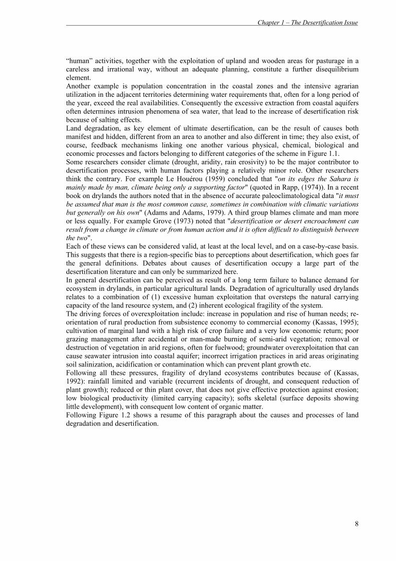
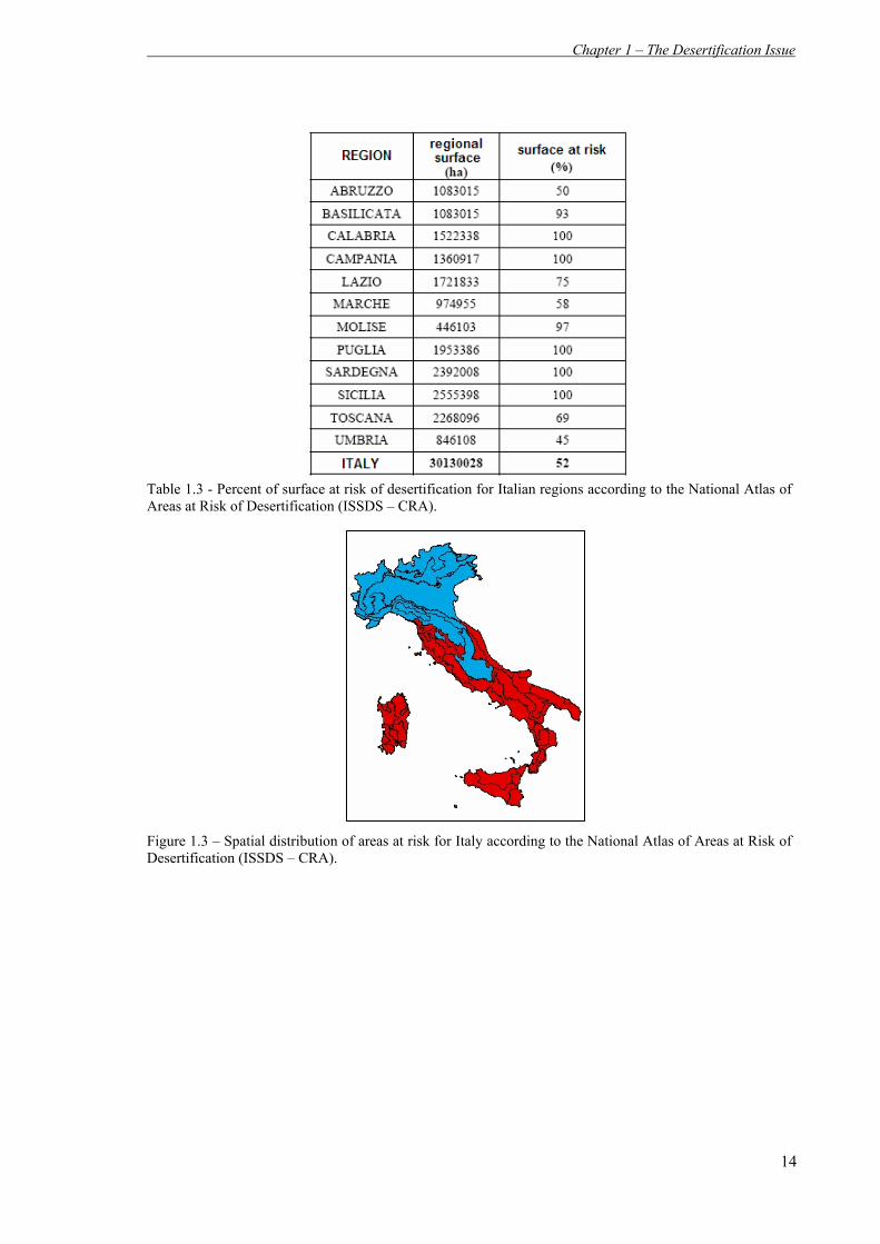
Practically there are two land use practices responsible for most of the world’s land degradation: deforestation to create cropland in the humid regions, and overgrazing in the drylands (UNEP, 1992). Soil erosion is the greatest problem in rain-fed cropland (affecting 47% of the land) whereas salinity and waterlogging are the main problems in irrigated drylands, affecting 30% of the lands (Glenn et al., 1998; Kassas, 1995). It is predicted that global warming will increase the area of desert climates by 17% in the next century. The area at risk of desertification is thus large and likely to increase, damaging in particular agricultural areas (UNEP, 1992).Worldwide, desertification is making approximately 12 million hectares useless for cultivation every year. Desertification and the consequent degradation of vulnerable ecosystems are problems that occur in all the European countries of the Northern Mediterranean, which is a complex mosaic of diversified landscapes. These Mediterranean countries such as: Spain, Portugal, Italy and Greece are considered by the UNCOD as potentially degraded areas. In a Mediterranean context, desertification is considered as the consequence of a set of important processes, active in arid and semi-arid environments (Kosmas et. al, 1999). In particular, among all the previously cited processes of desertification, water erosion is the most intense and widespread in Europe (Poesen, 1995). The area of land with a high water erosion risk in the southern EU member states is remarkable (CEC, 1992), equal to about 10% of the rural land surface. As in most other semi-arid regions, desertification in the Mediterranean region is largely a human-driven problem, which can be effectively managed only through a thorough understanding of the principal ecological, socio-cultural and economic driving forces associated with land use and climate change, and their impacts (MedAction, http://www.inea.it/medaction/documenti.cfm). Mediterranean land degradation is often linked to poor agricultural practices. Soils become salinized, dry, sterile and unproductive in response to a combination of natural hazards - droughts, floods, forest fires - and human-controlled activities, especially overgrazing. The situation was aggravated by the social and economic crisis in traditional agriculture in recent years and the resulting migration of people from rural to urban areas. The result is abandoned land, particularly on marginal and easily eroded hillsides, and weakened agricultural planning and land management. The modern economy is also contributing to the problem. Fertilizers, pesticides, irrigation, contamination by heavy metals and the introduction of exotic (invasive) plant species is undermining the long-term health of the soils of the region. Physical changes imposed on watercourses by the construction of reservoirs, the canalization of rivers and the drainage of wetlands are affecting land quality. Meanwhile, groundwater levels are declining widely, resulting among other things in saltwater intrusion into coastal aquifers. Some 80% of the region‘s available freshwater is used for irrigation. The dramatic and continuing growth of industry, tourism, intensive agriculture, and other modern economic activities along the coastlines is placing particular stress on coastal areas. For that concerning Italy, various combinations of predisposing physical factors (aridity, drought, rain erosivity, morphology, orography, highly erodible soils) have augmented in our country the effects of degradations together with human pressures. Indeed Italy shares with the northern Mediterranean countries many of features above described. In particular the desertification interests the areas of southern Italy (Sicily, Sardinia, Calabria, Apulia, Basilicata regions) exposed to climatic and human stresses. Also the central-northern regions (Tuscany, Emilia Romagna, and the Po river valley in general) show a deterioration of the climatic conditions and they are more and more susceptible to irregular precipitation, drought and aridity. It was estimate that the 52% of Italian territory (Table 1.3) is exposed to risk of degradation processes: this is the study area considered for the production of the National Atlas of Areas at Risk of Desertification (supplied by the Istituto Sperimentale per lo Studio e la Difesa del Suolo - CRA), territory largely coincident with Mediterranean biogeographic region (EEA, 2002) and divided according to following Figure 1.3.
Chapter 1 – The Desertification Issue
14
Table 1.3 - Percent of surface at risk of desertification for Italian regions according to the National Atlas of Areas at Risk of Desertification (ISSDS – CRA).
Figure 1.3 – Spatial distribution of areas at risk for Italy according to the National Atlas of Areas at Risk of Desertification (ISSDS – CRA).
Chapter 1 – The Desertification Issue
15
1.3. Actions against desertification
1.3.1. World action After stating that land degradation and desertification constitute a great problem with dramatic environmental, social and economic consequences, and after severe and protracted drought interesting African countries, the UN General Assembly decided to hold a UN Conference On Desertification (UNCOD) in 1977 in Nairobi (Kenya). The Conference produced a Plan of Action to Combat Desertification (PACD), a technically elaborate document: 28 recommendations each detailing actions to be carried out at the international, national and regional levels. The Action Plan became the framework for national and international action for the next 15 years under the general guidance of UNEP. These efforts reached a turning point with publication of the first edition of the World Atlas of Desertification (UNEP, 1992), which resulted in a revised edition (UNEP, 1997), and a subsequent series of program reviews (Dregne et al., 1991; Kassas, 1995). Despite the initial optimism, because of scarce resources, the implementation of PACD was limited. The United Nations Conference on Environment and Development (UNCED, known as Earth Summit, Rio de Janeiro, June 1992) produced an action-oriented document: AGENDA 21. In its final version it represents a world consensus on what needs to be done. Chapter 12 Managing fragile ecosystems: combating desertification and drought, addresses problems that are directly related to our subject providing guidelines for elaboration of national plans of action for (1) managing of drought and (2) combating land degradation. In 1994 the United Nations Convention to Combat Desertification (UNCCD) was signed in Paris, France, and entered into force on 1996. The aim of this treaty is to prevent and reduce land degradation, rehabilitate partly degraded lands and reclaim desertified ones. It deals with the extensive desertification phenomena of the northern Mediterranean countries and also addresses the problem in Central and Eastern Europe. The actuation of the Convention is at regional, sub-regional, national and local levels. For this reason, the Convention is completed by four annexes supplying guidelines to apply it in menaced territories, grouped into 4 geographic areas: Africa, Asia, South America/Caribbean, North Mediterranean. The elaboration and implementation of Regional Action Programmes (RAPs) and National Action Programmes (NAPs), form helpful policy instruments to combat desertification and soil degradation phenomena in these areas. Until now, over 170 countries have accepted the Convention clearly demonstrating the global nature of the problem of desertification.
1.3.2. European Actions It is specifically recognized that desertification and consequent land degradation are occurring in areas of Portugal, Spain, Italy and Greece. The European Commission and its northern Mediterranean member states are signatory partners of the UNCCD. Indeed a sub-regional group (Greece, Italy, Portugal, Spain and Turkey) has already prepared and launched a Subregional Action Programme (SRAP) with the aim of delineate common strategies and programs, not only cooperating together with the Developing Countries but also by means of planning and intervention at regional, sub-regional and national levels. At regional level, activities are being undertaken particularly through the establishment of regional thematic networks for scientific cooperation. European Commission (EC) promoted several activities for improving European research about desertification, by means of the Six Framework Programme (FP6), for the period 2003-2006. The section devoted to mechanism of Desertification focuses on “study the driving processes of the desertification in the framework of likely scenarios of multiple stresses driven by land use changes and climate changes and development of methods and tools to achieve an integrated assessment”. A great importance is given to the identification of indicators useful to assess the effects of land degradation and to the development of advanced modelling tools and actions. Furthermore, it is also established that all these strategies have to be developed in areas relevant to the UNCCD.

Chapter 1 – The Desertification Issue
16
Moreover, specific desertification research efforts at the European scale were also promoted by the EC including projects which have involved researcher from universities and research centres of different European countries working together and using an interdisciplinary approach in order to take into account all aspects concerning desertification. These projects focused their efforts on providing reliable data and information sources, to increase the understanding of the causes of desertification, in order to forecast and combat it, as well as to mitigate the effects of on-going processes. The studies were carried out both at local and at regional scale, and environmental and socio-economic factors characteristics of the Mediterranean area were taken into account. EU members are also investing in the systematic monitoring of land degradation, although there is still a need for a better coordination of the collection, analysis and exchange of data, including the countries outside the EU.
1.3.3. Italian Actions Italy is considered to be one of the countries affected by desertification as comprised in the Annex IV of the UNCCD. At national level the Convention provides that these nations are adopting specific NAPs (National Action Plans). In 1997 the Italian government instituted the National Committee to Combat Drought and Desertification (CNLSD, Comitato Nazionale per la Lotta alla Siccità e alla Desertificazione), with the task of coordinating the actuation of Convention. The committee includes components representing different cultural realities with the aim of facing desertification in its environmental, social, economic and scientific aspects. The main principle of NAP is implement the interventions and their integration both at national and local level. The NAP provides that the Region governments and the River Agencies find in their territory the areas vulnerable to desertification and define proposals of intervention to adopt in these areas, focusing on four main sectors:
- soil protection; - sustainable resource management; - reducing impact of productive activities; - re-equilibration of the territory.
The NAP focus over a fundamental concept, the desertification vulnerability: if it is easy to understand a desertified area, as it is sterile, it is more difficult to detect an area vulnerable to desertification and even more at risk of desertification (see Chapter. 2 for vulnerability/risk distinction).
1.4. Desertification as a research issue
1.4.1. First approaches Desertification has been the subject of much activity and research in the physical sciences, inside four main broad areas (Thomas, 1997): i) attempting to assess, as reliably as possible, the extent and nature of the problem and the rate at which it might increasing or diminishing (at global, national and regional scale); ii) attempting to identify the physical processes of desertification in order to understand how systems subject to degrading disturbances actually function and change; iii) aiming to identify appropriate remedial actions to stabilize or recover lands subject to desertification; iv) to assess the relationship between desertification and environmental problems and natural hazards occurring in drylands, including recent explorations of the position of desertification in the context of predicted anthropogenically-induced global climate changes. Despite the link with the physical sciences, desertification, with its social impacts and human causes, is also an issue in the domain of the social sciences. Desertification assessment has shifted from simple evaluation of the interannual movement of the desert boundaries to complex multivariate field surveys, to practical methodologies based on indicators of ecosystem functioning (e.g. rain use efficiency).

Chapter 1 – The Desertification Issue
17
Lamprey (1975) attempted to quantify the rate of advancing of the Sahara by comparing the location of the southern margin at two different times: the year 1958, according to a vegetation map produced by Harrison and Jackson (1958), and the year 1975, according to aerial and terrestrial surveys conducted by Lamprey (1975). During this 17 year period, he observed a 90–100 km displacement, thus concluding that desert edges were encroaching at about 5.5 km per year. This prompted many, a posteriori ineffective, anti-desertification actions. After Sahelian tragedy in early 70s’, desertification studies diversified using multidimensional methodologies. For example, the FAO/UNEP (1984) method was summarized by a matrix whose rows are quantitative and qualitative variables of vegetation and soil. The columns are classes of degree of desertification (slight, moderate, etc.). The elements of the matrix are, in the case of quantitative variables, the range of values of each variable corresponding to each degree of desertification status (Table 1.4). In the case of qualitative variables, there are verbal descriptions instead of values. Individual sites whose desertification status needs to be determined are visited and actual values or descriptions are recorded. The elements of the matrix are then integrated in an unexplained way into a single index that summarized the desertification status of a site into one of four classes: slight, moderate, severe and very severe (Table 1.4). The most well-known result produced by this approach was the estimation that 70% of all drylands were affected by desertification (UNEP, 1992).
Table 1.4 – FAO’s matrix. Example of the criteria for the evaluation of the desertification status proposed by FAO/UNEP (1984) But this methodology presents at least two problems: the first one is the subjectivity if data are not a measure, the second one is that this is a time-consuming methodology. Furthermore, this methodology is diagnostic but not prognostic.

Chapter 1 – The Desertification Issue
18
Then we can understand how the need to develop a practical and objective methodology based on indicators which were applicable and readily interpretable across different regions was an important lesson from the 1980s and early 1990s attempts.
1.4.2. The indicators In the sphere of dealing with desertification, the European Environmental Agency introduced the use of indicators as “parameters or values derived by other parameters, supplying numerous information relative to a phenomenon. They are quantitative information that help in explaining how some situations or conditions evolve in the space and in the time. The indicators often simplify the reality with the aim of quantify several phenomena and of communicating them” (Gentile, 1999). The indicators are very useful to efficacy describe some complex processes unless difficult to measure or observe (Rubio and Bochet, 1998). We can define an indicator in several ways: variable, parameter, measure, statistical measure, fraction, value, index etc. In general it can be both quantitative and qualitative. Indicators can be further aggregated in indices allowing a simultaneous evaluation of different changing factors; moreover they can be used to elaborate responses and actions and to predict future impacts of human activities over the environment and society. It is possible to use indicators to: i) determine conditions and environmental changes in respect to the society and development processes; ii) analyze causes and effects in order to supply useful decisional tools for responses to and prevention of a phenomenon; iii) individuate trends to predict potential impacts of human activities to decide future political strategies. We can know indicators at different spatial scales: local, national and continental. The chosen scale influences the observation duration of the phenomenon, moreover the data gathering to create indicators has to be based over a network of observations that will be representative for various systems over which the land degradation process acts. At this time, thanks to Remote Sensing and GIS disciplines, more and more indicators can be generated directly at the desired scale. It is fundamental to know what kind of indicators are more appropriated for each scale. The indicators have to be temporally sensible to changes. If we consider those characteristics of systems prone to degradation that modify themselves in few weeks or in many years, we have not an appropriate indicator. In general, the best indicators about the quality and degradation of the various system components are the ones showing significant changing in few years. We have also to specify that the validity of an indicator changes if they change also the data used to evaluate it. We can observe, indeed, that some characteristics change very slowly (e.g. topography and stream network), other ones in mid-term (e.g. vegetation and type of erosion), other ones very fast, as seasons or one year (e.g. soil moisture and grazing management). At this regard researchers speak of “fast” and “slow” variables. In terms of biophysical variables, crop yield, for example, would be a fast (or quickly changing) variable whereas soil fertility, which affects yield, is a slowly changing variable. In terms of socio-economic variables, household debt would be a fast variable whereas market access, which affects debt, is a slowly changing variable. Anyway, it is clear that, in the context of desertification, the indicators are variables that show the land degradation, but not necessarily are able to “control” it. The complex desertification phenomenon, caused by different and interrelated factors, cannot be described by a single indicator or measure (e.g. aridity index) but we need a set of indicators, each one describing an aspect of the process (Enne and Zucca, 2000). Various research projects and national institution efforts proposed some indicators and models to organize them, in particular within specific target areas (e.g. in the European projects MEDALUS (Mediterranean Desertification And Land Use), MEDACTION (Policies for land use to combat desertification) and DESERTLINKS (combating DESERTification in Mediterranean Europe: LINKing Science with Stakeholders)). Indeed while earlier research work was more concentrated on the physical dimension of desertification, the focus has been adjusted more on the involvement of local stakeholders and research on social, economic and institutional dimensions of desertification. In connecting these

Chapter 1 – The Desertification Issue
19
multi-disciplinary dimensions of the desertification problem, much knowledge has been gained on suitable indicators, such that European research has led to substantial progress in this field. In particular, we should remember that DESERTLINK project (http://www.kcl.ac.uk/projects/desertlinks/) developed a system of key indicators (Desertification Indicator system for Mediterranean Europe (DISforME)), and it is a very useful tool for monitoring desertification processes in Mediterranean area and for helping in decision support system.
1.4.3. D.P.S.I.R. framework The logic model known as DPSIR (Driving force-Pressure-State-Impacts-Responses), developed by the EEA and showed in Figure 1.4, was used to classify efficiently the information and to identify that key set of indicators better describing desertification phenomenon and the relationships and feedbacks among them.
.
Figure 1.4 – Relationship among various indicators (and their description) according to DPSIR framework The DPSIR framework is fundamental to organize information about environmental state. It assumes relationships of cause-effect among the social-economic and environmental components. The STATE indicators give an indication about the degradation of the lands at a given time. They can be qualitative and quantitative indicators, relative to the environment quality and determine its status from a temporal, spatial and functional point of view.

Chapter 1 – The Desertification Issue
20
The PRESSURE indicators are related to dangerous effects tolerated by the environment under various type of pressure (physical, human, etc.). The knowledge of pressures presupposes the estimation of determinant factors. These indicators derive by DRIVING FORCES. This category of indicators represent the anthropogenic activities and the various processes having an impact on the land degradation. In general they give a general indication of the causes of the changes in land degradation. Anyway they are principally indicators related to human activities as: intensive agricultural practices, overgrazing, population, tourism increase etc. The IMPACT indicators describe the result, both onsite (soil loss, poverty etc.) and offsite (flood, channel fulfilment) of land degradation and desertification. The RESPONSE indicators are linked to the corrective actions used to improve the STATE and to reduce the PRESSURES that influence the STATE. This type of indicators are functional to the protection programmes against desertification. They have the role of “measuring” the actions and the policies utilized to mitigate the human pressures and other factors contributing to desertification process. But we have to keep in mind that many indicators can be considered at the same time driving forces, pressures, impacts or responses.
1.4.4. Projects regarding desertification To help governmental institutions in assessing, knowing and looking for solutions to face land degradation, it is needed a precious contribution from research activities, involving many different disciplines. The Global Environmental Facility (GEF), created to provide funding to developing countries and countries in transition for measures that supply global environmental benefits, in partnership with the Food and Agriculture Organization of the United Nations (FAO), the United Nation Environment Programme (UNEP), the Global Mechanism of UNCCD and other partners, has provided resources to catalyze an international undertaking in supporting LADA (LAmd Degradation Assessment in drylands) project in order to develop and test an effective assessment methodology for land degradation in drylands, using the DPSIR scheme. The main aims of the assessment of LADA project are: 1) to identify the status and the trends of desertification;
2) to highlight the hotspots of degradation (the areas with most severe land constraints); 3) to underline the brightspots, thus the areas where actions have slowed or reversed the degradation or the priority areas where the conservation and rehabilitation could be most cost-effective.
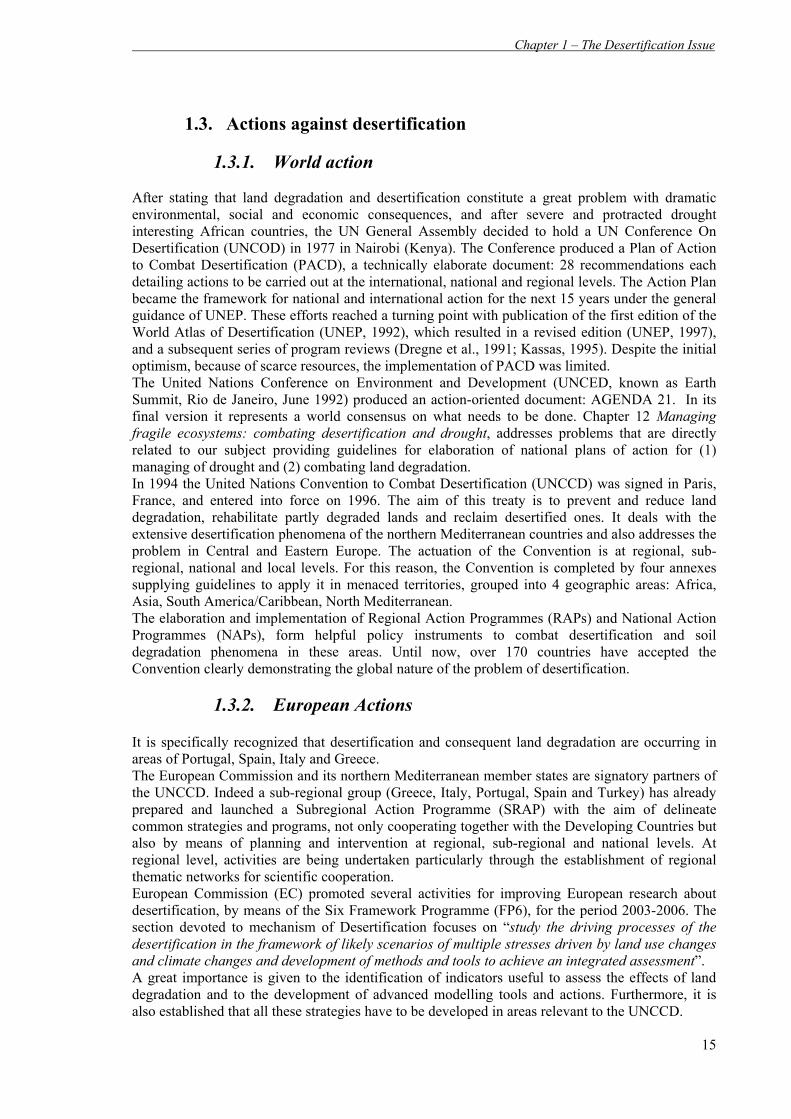
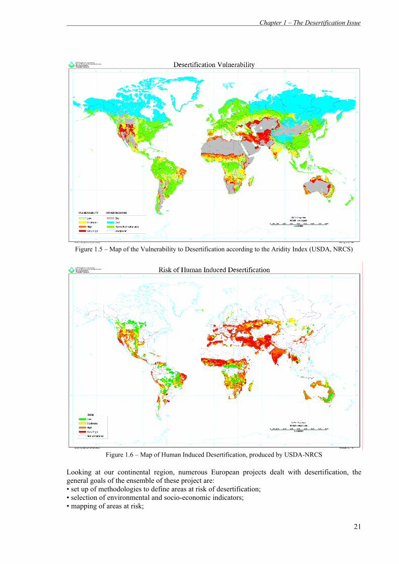
The U.S. Department of Agriculture, Natural Resource Conservation Service (USDA-NRCS) produced a Desertification Vulnerability Map according to climatic regime (Figure 1.5) distinguishing it by the Risk of Human Induced Desertification (Figure 1.6), the two main categories of factors we have already individuated.
Chapter 1 – The Desertification Issue
21
Figure 1.5 – Map of the Vulnerability to Desertification according to the Aridity Index (USDA, NRCS)
Figure 1.6 – Map of Human Induced Desertification, produced by USDA-NRCS Looking at our continental region, numerous European projects dealt with desertification, the general goals of the ensemble of these project are: • set up of methodologies to define areas at risk of desertification; • selection of environmental and socio-economic indicators; • mapping of areas at risk;

Chapter 1 – The Desertification Issue
22
• assessment of the most important land degradation processes; • implementation of monitoring systems; • individuation of measures for preventing or reducing the vulnerability or to adapt the lands; • development of Decision Support Systems (DSS); • analysis of future scenarios. Among various European projects, the MEDALUS (http://www.medalus.demon.co.uk/) is the one into which it was developed ESA methodology (Kosmas et al. 1999), a consolidated procedure representing today an international reference standard. Briefly, we can say that for each of the four components considered to be related to desertification (soil, vegetation, climate, land management) the most important variables are taken into account in order to represent sensitivity of the component itself. Each variable has to be divided into classes of increasing predisposition to desertification and to each class it is assigned a weight expressed over an homogeneous scale, generally comprised between 1 (no predisposition) and 2 (full predisposition). Clearly, this classification has to be done by experts in different disciplines. Then it is calculated the geometric mean among the variables inside each factor. In this way we obtain a specific index for each considered factor: Soil Quality Index (SQI), Climate Quality Index (CQI), Vegetation Quality Index (VQI) and Management Quality Index (MQI). This set of indices is again synthesized to obtain an ESAI (Environmentally Sensitive Area Index) according to the following relationship: ESAI = (SQI * CQI * VQI * MQI)1/4
In the next Figure 1.7 we can see an example of the scheme of application of the ESA model.
Figure 1.7 – Scheme of the ESA methodology
Also the JRC (Joint Research Centre) jointly with the INEA (Istituto Nazionale di Economia Agraria) produced a Map of areas sensible to desertification (Figure 1.8) for countries of Annex IV of the UNCCD (Portugal, Spain, Italy, Greece, Turkey), using the same above described approach.
texture, mother rock, stoniness, depth, drainage gradient…
Precipitation, aridity, exposition…
fire risk, protection against erosion, drought resistance, vegetation cover…
VARIABLES
Land use intensity, protection policies…
SOIL QUALITY INDEX (SQI)
CLIMATE QUALITY INDEX (CQI)
VEGETATION QUALITY INDEX (VQI)
MANAGEMENT QUALITY INDEX (MQI)
Index ESAII

Chapter 1 – The Desertification Issue
23
Figure 1.8 – Sensible Areas to desertification for the countries of Annex IV of UNCCD
The Project DISMED (Desertification Information System for the MEDiterranean, http://dismed.eionet.eu.int/index.html), coordinated by UNCCD in collaboration with the EEA, produced the Map of Sensitivity to Desertification Index (SDI, Figure 1.9), based on aridity index computation.
Figure 1.9 – Sensitivity to Desertification Index (SDI) map
The project DESERTLINKS, as already said, allowed the compilation of a Desertification Indicator System for MEditerranean areas (DIS4ME) and gives access to around 150 indicators of relevance to Mediterranean desertification. It has been designed to provide a tool to enable users from a wide range of backgrounds (including scientists, policymakers and farmers) to:
1. identify where desertification is a problem; 2. assess how critical the problem is; 3. better understand the processes of desertification.
Other important project are: • Project MEDACTION (http://www.icis.unimaas.nl/medaction/)

Chapter 1 – The Desertification Issue
24
• Project GEORANGE (http://www.georange.net/start.html) • Project REMECOS • Project LADAMER • Project REACTION (http://www.gva.es/ceam/reaction/) • Project DESERTWATCH (http://dup.esrin.esa.it/desertwatch/) • Project INDEX (http://www.soil-index.com/english/home.php) • Project DESERTSTOP(http://www.soilindex.com) • Project RECONDES (http://www.port.ac.uk/research/recondes/) • Project DESURVEY (http://www.desurvey.net/) • Project REDMED (http://www.gva.es/ceam/redmed/) • Project DESIRE (http://www.desire-project.eu/index.php) As already explained, Italy is one of the countries of Mediterranean area interested by desertification phenomenon. For this reason, Italian research institutions have been involved in many European projects regarding desertification. In general studies regarding the mapping of desertification risk in Italy were already carried out starting from global (Eswaran and Reich, 1998), continental (DISMED, 2003), national (CNLSD, 1998) and regional scale (UNCCD-CRIC, 2002). The first document about the desertification risk in Italy was the Map of Sensible Areas to Desertification (Carta delle Aree Sensibili alla Desertificazione) at scale 1:250’000, produced inside the CNLSD activities (Figure 1.10). With the aim of identifying the sensible areas to desertification, they have been considered following indices: • climate; • soil; • land use; • human pressures.
Figure 1.10 – Procedure for the identification of sensible areas by CNLSD

Chapter 1 – The Desertification Issue
25
From this analysis the national territory was divided into areas with none, low, medium, high sensibility (Figure 1.11).
Figure 1.11 – National Map of areas sensitive to Desertification
The prone areas have been detected by means of the annual average of the Aridity Index for the period from 1961 to 1990. The estimated vulnerable areas are 5.5% of the Italian territory, among Sardinia, Sicily, Calabria, Basilicata and Apulia regions. Other cartographic approaches have been conducted at sub-national scale using modified MEDALUS approaches: in Sardinia (Motroni et al., 2004), in Basilicata (Ferrara et al., 2005), in Tuscany (DESERTNET project), in Apulia, in Sicily and in Calabria (Iovino et. al, 2005). All these experiences applied ESAI methodology, with some changes whit respect to the original model according to specific characteristics of the studied areas. More recently, still using the MEDALUS approach, the EEA (DISMED, 2003) and FMA (Applied Meteorology Foundation) worked out a new map of the desertification risk in Italy at 1:1’250’000 scale, showed in the following Figure 1.12, where only the climate, soil and vegetation are taken onto account from the ESAI methodology.

Chapter 1 – The Desertification Issue
26
Figure 1.12 – Areas sensible to desertification in Italy
In the next example (Figure 1.13), on the contrary, also Management Quality Index (MQI) is considered in mapping desertification vulnerability (APAT-CRA/UCEA-CNLSD, 2006). In particular, here the ESA Index refers to 1961-1990 period, as the climatic data can be referred to that time.
Figure 1.13 - ESAI calculation for the Italian peninsula
Other approaches have been developed, for example the one of Pimenta et al. (1997), developed initially for the Portugal but then also applied to some Italian regions with interesting results. For this approach three indices are considered (Climatic Index, Soil Loss Index and Drought Index) and combined together in order to identify the most sensible areas. During the period 2003-2004, the ISSDS (Istituto Sperimentale per lo Studio e la Difesa del Suolo) and the Istituto Nazionale di Economia Agraria (INEA) produced the “National Atlas of Desertification Risk”, consisting in national databases and useful indicators. The Atlas represents a photograph of the state of the environment as respects to desertification.

Chapter 1 – The Desertification Issue
27
According to the CLIMAGRI project driven by the Central Office of Agricultural Ecology (UCEA-Ufficio Centrale Ecologia Agraria) of the Agricultural and Forestry Italian Ministry, the areas prone to desertification could be huger than those individuated by first tentative of CNLSD on the Map of Sensible Areas to Desertification. In particular in this context the desertification risk is evaluated as respects the climate change impacts over agricultural systems. The new aspect introduced by the CLIMAGRI project in dealing with desertification was the use of statistical analysis (Principal Component Analysis) in order to assess the relative influence of different predisposal and quickening factors that are combined (Figure 1.14) and to eliminate redundant information.
Figure 1.14 – Scheme of the procedure of CLIMAGRI project
The more prone regions to soil/land degradation resulted, anyway, Sardinia, Sicily, Calabria, Basilicata and Apulia. In particular, the results of this study indicate the Sicily and the Sardinia as the regions where the degradation processes are more advanced, because of, respectively, the scarce or absent vegetation cover influencing negatively soil erosion and the predominance of overgrazing. In conclusion we can say that, if seen together, the elaborated cartographies to map desertification at national and sub-national scale supply different results about the extension and localization of the risk, depending mainly by the scale and the detail of data used as input. Among the European project already cited, there are several “national” project producing useful instrument for desertification knowledge and facing. • Project DESERTNET (http://www.uniss.it/nrd) • Project RIADE (http://www.riade.net) • Project MEDRAP (http://uniss.it/nrd/medrap/index.htm) • Project RIMBDES (http://geolab.unifi.it) Finally, the SIDES project (SIstema informativo integrato per il monitoraggio, la valutazione, la mitigazione dei fenomeni di DESertificazione nelle aree italiane particolarmente affette) has the aim of produce an Informatic System to analyze and evaluate different types of data and information necessary to study desertification. Practically the problem is faced taking into account, at the same time, different aspects (about soil, vegetation, climate and land management) of the territory. In this context also the changes are taken into account, because in changing indicators qualitatively and quantitatively, also the sensibility to desertification can change.

Chapter 2 – Desertification in the study area and new approach
28
2. Desertification in the study area and new approach
2.1. Introduction
In the context of desertification, the Mediterranean islands have been recognized as “hot spots” because of various forms of soil degradation they show (EEA, 2000). The research experiences carried out in these regions of Mediterranean highlighted the relationship between degradation and land-use, and the need to search and apply methodologies to mitigate the phenomenon of land deterioration. The work of this thesis was developed in the context of the project “Design and implementation of a G.I.S. (Geographic Information System) to monitor the areas of Sardinia at risk of desertification, with the specific indication of the components of this risk, included their parameterization” funded by Regional Government of Sardinia and developed in collaboration with Agriconsulting S.p.A. and ESRI Italia. In this chapter we will present first the study area, the island of Sardinia, and its conditions with respect to desertification, and then we will briefly introduce the two main previous studies that dealt with this issue in the study area, underlining both their limits and their main concepts on which we agree. In the second part of the chapter we will explain our approach to evaluate desertification, the heritage from other studied methodologies and the newness we would to add to better understand the phenomenon and help policy-makers in facing the desertification process.
2.2. The study area: island of Sardinia
2.2.1. General description of the area
The Island of Sardinia is characterized by a high variability of landscapes with their morphologic, pedologic and botanical characteristics due to a particular geologic and paleoclimatic history of the region. The total area of the region is 24’089 km2, it is situated at the centre of western Mediterranean and comprised between 38°51’52’’ and 41°15’42’’ N of latitude and between 8°8’10” and 9°50’8” E of longitude (from Greenwich). The population is about 1’631’880 of people (census National Institute of Statistics (ISTAT), 2001), and about one fourth is concentrated into the area surrounding Cagliari, the biggest town on the south of the island. The resident population increases up to more than 3’000’000 inhabitants in the summer, because of the very famous tourist attractions of the Island. The mean annual temperature is strongly influenced, besides by latitude and by insular conditions, also by orography (Raimondi et al., 1996). The mean values are comprised between 11°C and 17°C, with a minimum values in January and a maximum value in July-August. The precipitation regime is highly variable, with a maximum in the winter, often after autumns very rainy (Arrigoni, 1968). During the summer there is a very low (practically null) precipitation amount. In some areas on the south of the island there are yearly precipitations less than 500 mm, whereas into inner hilly areas we can find a precipitation amount ranging from 700 to 900 mm per year. Only over the most elevated zones, in the inner mountainous areas, we can find higher precipitation values (Raimondi et al., 1996). The soil moisture regime is almost everywhere xeric. The geologic and morphologic characteristics of Sardinia are highly variable. The Paleozoic basement mainly consists in metamorphic and granite rocks outcropping in the half eastern part and in the south-western part of the island (Carmignani et al., 1992). The limestone and the dolomite sediments of Mesozoic directly lay on above mentioned formation (Pala et al., 1982), and they outcrop in the central-eastern part of the region, in the area of the Gulf of Orosei, in the north-western sector (Nurra) and in a central-southern area (Ogliastra and Sarcidano).

Chapter 2 – Desertification in the study area and new approach
29
The Cenozoic outcrops are located principally inside the huge depression extending from north to south. They consist of volcanic products (andesites, rhyodacites, ignimbrites, tuffs) and of marine, lacustrine and continental sediments (sands, marls, limestone, conglomerates, clays). A basic volcanism (basalts) began at the end of Cenozoic until the Quaternary. Basaltic flows outcrop mainly at the centre of the island. Most Quaternary deposits consist in sediments of continental origin, represented by alluvial pebbly deposits and located in the most important plains. In the coastal areas there are, also if in a discontinuous way, marine deposits (conglomerate, organic limestone and sandstone), fossil and actual dunes and tin deposits. Both the high lithologic variability and the different morphologic processes, integrated in the complex structural situation of the island, consisting in the alternation of horst and graben (e.g. Campidano depression), divided the territory into numerous morphologic regions with different characteristics: 18.5% is mountain, 67.9% is hill and 13.6% is plain (Pracchi e Terrosu Asole, 1971). The highest relief is the Gennargentu chain, touching the maximum elevation with the peak La Marmora (1834 m asl). The Sardinian soils are very different according to substrate, morphology, vegetation cover and land use (Aru et al., 1991). Only the 18% of the territory is covered by soil susceptible to irrigation: 3% by highly susceptible soils, 6% by moderately susceptible soils, and 9% by low susceptible soils. These soil are located in the internal and coastal plains, mainly over alluvial deposits of Pleistocene and Olocene, and are interested by an intensive agricultural activity, with or without irrigation. On the left part of the territory there are marginal areas for intensive agriculture showing strong limitations, but they are very important for particular crops, pasture and forest activities. The main land cover types are grassland and grazing land (almost 40% of the island's surface) and Mediterranean “macchia” (more than 20% of the surface). Hardwood forests cover almost 10% of total surface. The Sardinian flora is constituted by about 2000 species (Valsecchi, 1986) with dominant sclerophyll and xerophilous species, whose distribution is conditioned by climatic, geo-pedologic and morphologic characteristics. Inside the floristic composition the Mediterranean species dominate, and elevated is the number of endemic species. The autochthon forest formations consisting in Quercus ilex, Quercus pubescens and Quercus suber, with pure or mixed populations. As we can understand from the above description, the Sardinia falls into the biogeographic region with Mediterranean characteristics (Figure 2.1), more or less the same interested by desertification phenomena according to the National Atlas of Areas at Risk of Desertification (see Chapter 1, par. 1.2.5).

Chapter 2 – Desertification in the study area and new approach
30
Figure 2.1 – Biogeographic regions of Europe, with localization of the region of Sardinia
2.2.2. The desertification phenomenon in Sardinia
Among the main causes of desertification in Sardinia there are the drought periods, the overexploitation of groundwater and its consequent salinization, the high frequency and extension of firewood, the reduction of vegetation cover and the agricultural land abandonment. In respect to the other Italian regions at risk of desertification, we have anyway to specify that wider areas are subject to protection by laws. The areas more prone to desertification are the internal ones, in relation with the geo-pedology, the morphology and the type and intensity of human pressures. In this areas, the irrigation agricultural practices, if associated to a compatible management and to a more correct usage of water, could subtract several part of the territory to land degradation. But among the others, the most serious causes of land degradation/desertification in Sardinia are unquestionable: soil erosion and overgrazing that are strongly interrelated. If we think at DPSIR framework and its categories, we can recognize that here, for example, as the market asked for large quantities of cheese (Pressure), the result was the increase of cattle loading (Responses). This led to an increase of areas for the breeding, obtained through fires or ploughing (Driving forces) to cultivate on every kind of slope (State), having as consequence the soil degradation (Impact). Figures 2.2 show an example of this practice in various sectors of Sardinia.

Chapter 2 – Desertification in the study area and new approach
31
Figures 2.2 – Images showing an example of diffuse practice of ploughing over steep slope in various areas of the Island This aspect, fundamental for the assessment of soil degradation, is visible also comparing two maps of soils of Sardinia, the former for 60s’ and the latter for 90s’, where we can identify the clear increase of rocky outcrops and of shallow soils. Further, the economic gain apparently reached through the selling of a great quantity of cheese, whose incomes allow the reduction of deficit for the import/export balance of the region, in reality is contrasted by the loss of natural resources, and then it is not a real gain. Also as regards the tourism and the forestation, often the decisions are taken without adequate susceptibility and suitability studies aiming to compare the land use and the land quality requirement. Several works were carried out in Sardinia highlighting the presence of different factors and processes of soil degradation (chemical, physical, biological), as showed by Figure 2.3 (from Vacca et al., 2003), all these giving a contribution to general land degradation toward ultimate desertification.

Chapter 2 – Desertification in the study area and new approach
32
Figure 2.3 – Factors and processes of soil degradation in Sardinia
These degradation factors, specific of the soil, trigger other processes by inducing the variation of one or more soil properties in its fundamental attributes for life. From the land degradation point of view, involving not only soil but also other components of ecosystem, the driving factors in Sardinia are principally anthropogenic and can be aggregated into three principal groups: agricultural/pastoral/forestry activities, industrial activities and urbanization and they will be briefly analyzed only in their most evident aspects. These aspects will be then better developed and explained later in the thesis.
2.2.2.1. Agriculture
In the last decades, the national and European policies and markets imposed production choices inadequate (for extension and crops) to natural suitability of the territory, with consequent negative impacts. The intensive agriculture impacts on soil and water, in particular, by means of: - the uncontrolled use of fertilizer and pesticides that pollute superficial and underground water; - the overexploitation of water that causes its salinization and this water, if used in irrigation, has negative consequences on soil characteristics and on crops; - the strong mechanization that compacts the terrain, limiting soil permeability and infiltration and favouring erosion and runoff.
2.2.2.2. Pastoral activities
The breeding in general and the one of sheep in particular is an economic mainstay of the region. The main impacts of “overgrazing” are the defoliation and the plant destruction, the removal of nutrients and soil compaction, all leading to a change in hydrological balance of soil. But grazing is related to other factors: the amelioration techniques applied in Sardinia to improve pasture and to meet the needs, consisting in bush cutting, ploughing and seeding, increased the loss of soil in large portions of the island. As these areas are mainly located on moderately steep to steep slopes, it was observed that in autumn, after the first heavy rains, the shallow soils are eroded to the extent that, in many cases, the bedrock appears as rock outcrops (Vacca et al., 2003). Following Figure 2.4 shows this phenomenon in the area of Irgoli (North-East part of the island).

Chapter 2 – Desertification in the study area and new approach
33
Figure 2.4 – Example of erosion phenomena (left) in a grazed area that lead to the outcrop of the rock inside the erosion channels because of the total loss of soil. Here uncontrolled grazing quickens the degradation process, in particular in areas already menaced by erosion. Further, the breeders frequently apply fires to shrublands and forests to create new grazing for their cattle, without added costs.
2.2.2.3. Urbanisation
Past studies about the direct effects and the extent of urbanization in Sardinia showed that the main consumption of soil is regards the most fertile ones (Soil conservation project – CNR, 1982) (Table 2.1), that is the coasts and coastal plains, which are areas once used for rainfed or irrigated agriculture (Aru et al., 1998). Taking as a reference the well known and widely accepted Land Capability classification system (Klingebiel and Montgomery, 1961), soils with functional sterility belong to the last class, the eighth, representing soils which are left set aside, and only considered for ecological purposes.
Table 2.1 – Consumption of agricultural areas after the urban and industrial expansion in the hinterland of Cagliari (modified from Aru, 2002). Furthermore, there is an uncontrolled urban development over irrigable soils, as urban speculation has invalidated the efforts for a correct agricultural planning. An example is the recent urban

Chapter 2 – Desertification in the study area and new approach
34
expansion of the town of Olbia, a famous tourist place on the north-eastern part of the island (Figure 2.5), that occupied a surrounding irrigable area.
Figure 2.5 – Example of expansion of urban areas in lands previously occupied by agriculture (modified from Aru, 2002).
In this case we can assert that, under an apparent development form, there are hidden enormous territorial damages and destruction of natural resources, for example also the coastal dunes are menaced by expanding of tourist complexes.
2.2.2.4. Quarrying and mining activities
Also the quarrying activities (often without planning) over the alluvial plains near the rivers menace mainly the soils with highest fertility. The uncontrolled extraction of materials by quarry cultivation in the alluvial plains has strongly modified the landscape leading to the irreversible loss of soil. Table 2.2 shows the result of a study relative to Santa Lucia river basin, from which we can notice that the soils interested by quarry activities are the ones falling into the best classes (I-II) of suitability.
Table 2.2 – Soil consumption due to quarry activity in the alluvial plain of Santa Lucia river (SW Sardinia) (after Puddu and Lai, 1995, modified).
Mining activities (historically for lead, zinc, iron, silver, barium, fluorite and antimony) are the most responsible for the soil pollution and consumption; recently (1980s) almost all the mining activities were abandoned and, then, the mineral dump, as unstable and prone to accelerated erosion, constituted a serious danger for soils, rivers, lakes and the sea, with the risk of an irreversible contamination (e.g. mine of Montevecchio, SW Sardinia).

Chapter 2 – Desertification in the study area and new approach
35
2.2.2.5. Water resources contamination
In Sardinia, because of its hydrologic deficit, the agricultural practices, and in particular the intensive ones need artificial sources of water for the crops. The seawater intrusion along the coastal area is caused by excessive exploitation of groundwater to satisfy the necessity of agriculture, industry and human needs. This problem arose in particular in the Gulf of Cagliari (APAT, sheet 557 of the Geologic Map of Italy at scale 1:50 000), in the Flumendosa river valley (APAT, sheet 549 of the Geologic Map of Italy at scale 1:50 000; Ardau et al., 2002; Lecca et al., 2004), at the Cedrino river delta and in the coastal area of Capoterra (Barrocu et al., 2001). This phenomenon leads also to soil salinization if water is used for agriculture and to degradation of territory, then large tracts of arable land have been abandoned.
2.2.2.6. Fires
In recent years in Sardinia breeders needed to create pastoral areas without additional costs. The necessity to enlarge the pasture areas is mainly influenced by the number of sheep, which has recently risen to over 3’000’000. This is also the reason why the use of fires to increase pasture areas is still common in Sardinia. Following Table 2.3 shows us that fires have increased in the decade 1984-1994.
Table 2.3 – General statistics of recent fires in Sardinia (source: Assessorato Difesa Ambiente – Regione Autonoma della Sardegna)
Table 2.4 explains us as grazing lands are the ones mainly interested by fires.
Table 2.4 – Average annual fires in Sardinia (source: Assessorato Difesa Ambiente – Regione Autonoma della Sardegna)
2.2.2.7. Soil erosion
In Sardinia there is a wide lithologic variety, with rocks different both for age and for mineralogical composition, and with a different degree of susceptibility to alteration. For example in landscapes with granites, quarzites, calcareous rocks and effusive rock, the desertification risk is increased by
Chapter 2 – Desertification in the study area and new approach
36
the slow alteration of this type of rocks, and by consequent major quantity of time necessary for soil formation. Other factors contribute to slow down the pedogenic process, mainly the climate and the human activities. Indeed accelerated erosion affects large portions of the hilly and mountainous areas subject to irrational agricultural, pastoral and forestry activities, such as deep ploughing, deforestation, exotic tree species plantation, overgrazing and the use of fires to increase pasture areas (Aru, 1984; 1985). These landscapes are subject to degradation but, if correctly managed, soil and vegetation cover could regenerate quickly. For example a recent study in an area of southern Sardinia (Rio s. Lucia Basin) confirmed the efficient role that vegetation cover has in facing erosion phenomena, whereas the areas with eucalyptus, because of not rapid growing, makes this cover type under the economic marginality (Vacca et al., 2000), and we have to take into account that almost 20’000 hectares have been planted in Sardinia with Eucalyptus sp.
2.2.2.8. Decline in organic matter
Reduction of organic matter content in the forest soil has been detected in many areas used for agricultural, pastoral, and forestry activities. For instance, in Gallura (north-eastern Sardinia) ploughing and repeated use of fires for clearing pasture areas in Quercus suber forests caused a significant decline in organic matter content. In these forests mainly used for cork production well-developed ectorganic horizons are always present, with a total thickness ranging from 5 to 10 cm, and the mineral soil is generally 50 cm deep. In these areas the organic matter content in the forest floor ranges from 1.76 to 3.72 kg/m2 (Vacca, 2000). In Quercus suber forests used mainly for grazing, the ectorganic horizons are very poorly developed, with a total thickness normally ranging from 1 to 3 cm, and the mineral soil is generally 20-25 cm deep. In these areas, the organic matter content in the forest floor ranges from 0.45 to 1.84 kg/m2 (Vacca, 2000). Trastu et al. (1996) measured 34 g/kg of organic matter in surface horizons of Quercus suber forests not subjected to ploughing, and only 15 g/kg in surface horizons of ploughed forests.
2.2.3. Previous regional experiences: state of the art
In the sphere of the arrangement of “Guideline for the national policies and measures for combating desertification and drought”, approved by CNLSD and after CIPE (Interministerial Committee for the Economic Planning) deliberation, the Autonomous Region of Sardinia activated a technical secretariat with the aim of producing the Regional Programme to combat desertification involving the political authorities and often local agencies. Among various approaches, we want to highlight the procedure developed by Costantini et al. (2004) and the one elaborated by ERSAT-SAR (Regional Agency for the Development and Technical Assistance in Agriculture - Regional Agrometeorological Service; Motroni et al., 2004). For the former, in particular, we focus our attention on the introduction of a difference among: - desertified lands that are intended as tracts of land occurring in dry climates and showing “functional sterility”, that is areas where agriculture and forestry are currently no longer either economically or ecologically sustainable; - vulnerable lands, where the environmental characteristics are close to those of desertified areas, but some factors, e.g. vegetation cover or irrigation, successfully mitigate the process of desertification; - sensitive lands that are surfaces where processes leading to desertification are active, although lands do not yet have functional sterility. In this first case, the Sardinia island was one of the validation areas of the EPIC (Environmental Policy Integrated Climate, former Erosion-Productivity Impact Calculator, Sharpley and Williams, 1990) model that was used to assess desertification, in the most general context of elaboration of

Chapter 2 – Desertification in the study area and new approach
37
the Atlas of the Desertification Risk in Italy. In this case the indicators reported in Table 2.5 have been taken into account, and they are divided into three of five categories of DPSIR framework:
Figure 2.5 – Indicators considered in assessing the areas sensitive and vulnerable to the risk of desertification and drought in Italy by EPIC approach.
The validation of the method was obtained by means of a set of field observations, stored in a specific database. Each observation was georeferenced and briefly described in terms of state and causes of desertification. A picture of the landscape and an aerial photograph of the site were added to the site information. The observation was linked to the geographic database and then information about geology, morphology, land use and soils of the sites (Figure 2.6) (Costantini et al., 2004).
Figure 2.6 - GIS of the true points for validation of the EPIC procedure in Sardinia
The other approach was the one used by the ERSAT, with the task of studying measures for an efficacious fight to these problems in respect to the NAP (National Action Plan) and the Regional Plan guidelines. ERSAT developed a monitoring programme together with the SAR for the “Realization of a Geographic Information System to individuate and monitor the areas sensible to desertification in Sardinia”. The work, that in a first phase produced a Map of areas vulnerable to desertification at scale 1:250’000 (in order to compare it with other already existing products) using the Portuguese methodology (Pimenta et al., 1997), then it carried out, at the same scale, a

Chapter 2 – Desertification in the study area and new approach
38
Desertification Vulnerability Map according to ESAI methodology (Kosmas et al., 1999, see Chapter 1 – Par. 1.4.4), that has been further detailed at a bigger scale (1:100’000), also if not for the entire region. For the product (whose scale of values ranges from 3 to 9 as it is a sum of three layer each one with 3 classes of severity) the result was that the 25% of the territory is at medium high/high risk, the 42% at medium risk and the left at moderate/low risk (Figure 2.7).
Figure 2.7 – Map of desertification vulnerability according to the Pimenta et al. (1997) methodology.
The ESAI methodology was applied using both bio-physical and socio-economic factors, modifying the original methodology in order to make it more compatible to the study area and with more detailed inputs according to the scale of work. In particular, remembering the ESAs approach scheme considering four categories: soil, climate, vegetation, land management, following indicators have been taken into account to derive from their geometric mean a quality index for each category: - SQI (Soil Quality Index) : mother rock, texture, stoniness, depth, drainage and slope; - CQI (Soil Quality Index): precipitation, aridity index and aspect of the hillslopes; - VQI (Vegetation Quality Index): natural fire risk, capacity of protection from erosion, resistance to drought and vegetation cover; - MQI (Management Quality Index): land use intensity and protection policies. Then, these four indices were operated together in order to derive a final index representing vulnerability to desertification and classified in the following way (Table 2.6), where the increasing number in the subtype class indicate the increasing severity of the relative state.

Chapter 2 – Desertification in the study area and new approach
39
Table 2.6 – Classification of the ESAI index (Motroni et al., 2004)
The cartographic results are consultable on the web through a GIS viewer (Figure 2.8): http://www.sar.sardegna.it/servizi/sit/esai250.asp?wgs=1 allowing also examining the four sub-index products.
Figure 2.8 – Web pages of SAR allowing the display of the Map of the Areas Sensible to Desertification (modified from Italian version)
The results showed in this case that more than half (51%) of the island territory is at risk, belonging into the macroclass defined “critical” and comprising the classes C1, C2 and C3, with increasing severity. Then the same methodology was applied at a more detailed scale (1:100’000) for 16 areas defined by official cartography at scale 1:100’000 (Figure 2.9), and then results were verified by field survey for each of these areas (Figure 2.10).

Chapter 2 – Desertification in the study area and new approach
40
Figure 2.9 – Map showing the results of SAR-ERSAT application at scale 1:100.000
Figure 2.10 – Field validation procedure for the SAR-ERSAT methodology
Both the approaches are implemented into the GIS environment and both are taken into account in order to develop and implement our methodology.

Chapter 2 – Desertification in the study area and new approach
41
2.3. The new proposed methodology
The Sardinian Borough Council Clerk’s Office for the protection of the environment has, besides the others, the goal to mitigate the actual desertification phenomena and to prevent the potential ones, to know their causes and to determine their temporal and spatial evolution. At this aim, the main objective of policy-makers joined with local agencies and researchers is to integrate the actual knowledge in order to understand where, how and how much the human activities and the socio-economic components contribute to trigger the process under study. For this reason, the Autonomous Regional Government of Sardinia funded the project called “Design and implementation of a G.I.S. (Geographic Information System) to monitor the areas of Sardinia at risk of desertification, with the specific indication of the components of this risk, included their parameterization” that started in February 2005, and whose framework and implementation is the topic of this thesis. Before to explain the adopted methodology, we should like focus the attention on our main objectives:
- to determine, at regional scale, the characteristics of the areas subject to desertification; - to evaluate the nature and the intensity of various components contributing to the phenomenon with a different influence; - to define the direct impacts of desertification; - to identify the necessary procedures both to develop an evaluation and monitoring method and to validate it; - to identify the most critical areas (hotspots); - to suggest solutions analyzing different practices of land management that generated the brightspots (areas where there was an amelioration); - to favour the diffusion and the exchange of information; - to promote the using of software applications as decision support tool.
To answer our questions first we took into account some particular features of several previous projects working on desertification, as the ones described in Chapter 1. In particular we chose to select multiple aspects of the phenomenon under study (e.g. MEDALUS, Kosmas (1999) and Pimenta et al. (1997) approaches), also considering a different significance for each of them (e.g. CLIMAGRI project’s approach). Then we decided to consider as starting point the usefulness of “indicators”, considering: i) the FAO/UNEP Methodological Framework used within LADA project, suggesting guidelines very functioning to evaluate degradation phenomena and using DPSIR framework to classify the indicators; ii) the DISforME indicator system developed inside DESERTLINKS project, and specifically suitable for the Mediterranean area. Starting from these assumptions we divided the work into six main phases: 1) assessment of the aspects of problem in the study area (already discussed in par. 2.2.2); 2) definition of the methodology; 3) collection and integration of useful ancillary data (DATABASE); 4) informatic organization and homogenization of data in a geographic environment (GIS DATABASE); 5) whole implementation of the methodology and detection of areas at risk (ASSESSMENT); 6) Development and diffusion of GIS tool to monitor desertification phenomena and to repeat results of the risk evaluation (ASSESSMENT) also a different scales and/or simulate its evolution implementing different cases (SCENARIOS). In the following we will explain the point 2), illustrating the motivation and the general procedure developed to satisfy all our objectives, leaving to next chapters the description of other points. To better understand the methodology, how to satisfy the project requests and the necessity to overcome the limits of earlier approaches, it is necessary to illustrate the main concepts and tools that we put at the basis of our choices, and that we decided to include into the new approach as improvement of previous ones: i) the understanding and the distinction between vulnerability and risk, ii) the use of GIS instruments and iii) the use of modelling in place of static indicators.

Chapter 2 – Desertification in the study area and new approach
42
2.3.1. Vulnerability and risk
Prior approaches developed in dealing with the issue of desertification focused their attention on vulnerability, with the meaning of “fragility of an area against the pressures of land degradation”. But the outcomes required by the project title (i.e. “….areas at risk of desertification…”), comprising the evaluation of processes and factors related to desertification, lead to necessity of a clear definition of both the Vulnerability and the Risk to which the territory can be subject, because these two aspects are often confused and misinterpreted. According to scientific literature (Brooks, 2003) these two concepts can be sharply distinguished: - the vulnerability is the attitude of an area to suffer damages and losses after a specific event;
- the risk is a measure of the damage in terms of value of various elements in the area that suffers from the phenomenon (it is the expected number of lives lost, persons injured, damage to property and disruption of economic activity due to the occurrence of the catastrophic natural phenomenon), and it is given by the value of element considered at risk multiplied by the vulnerability and by the hazard (the probability that an event can occur in a specific interval of time, often represented by the return period of the considered event).
In other words hazard expresses the natural phenomenon and risk its consequences over a territory with different degrees of predisposition or vulnerability. Obviously the risk is more difficult to estimate than hazard because it involves, in addition to the hazard, estimation of the vulnerability of the elements at risk. It becomes obvious from the above definitions that it is the risk and not the hazard that can be mitigated, mainly through the reduction of the vulnerability of the elements at risk. Hazard cannot in general be mitigated except for some climate related hazards (e.g. extreme temperatures, desertification) that may be moderated through long term measures affecting the climate itself. Therefore research for natural hazards must be targeted primarily towards risk mitigation, aiming to two broad directions: 1) better understanding the physics and mechanisms generating the natural hazards; 2) measures for reducing the vulnerability of the elements at risk (Anagnostopoulus, 2006). Obviously the first direction is the one on which we are here interested and then, in this study, we chose to consider the risk simply as the combination of the environmental vulnerability and the relative significance (type of land use) of the fragile areas, as we will see later. In this way, reduction of the vulnerability could be also considered as the increasing of the capability and proneness of a territory to bear and to face the event or to adapt itself to changes.
2.3.2. Why models?
Modelling is a more and more useful and diffuse instrument in environmental research mainly if associated with advanced GIS instruments at this time available. In general models simulate the effect of an actual or potential set of processes, and predict one or more possible outputs, that approximate in different measures the real progress of studied phenomena. Models are then used to describe, explore and analyze an evolving system, trying to represent it as much authentically as possible. They allow combining detailed data and information with the knowledge of processes and in this way to individuate the behaviour of the whole system. Using models requires decisions and compromises: the model is, first of all, a simplification of a real system very complex and then, to be calculated, requires further omitting all the factors considered irrelevant for specific objectives. In particular models could be more or less simple according to input data and complexity of the modelled process. In this context, the modelling approach was chosen not only to improving the knowledge of the structure and the function of the multifaceted issue of desertification, but also to give a contribution to political decisions. The necessity of using models in environmental research is based on the fact that even if more data can be collected in environmental field, on the other hand often it is not possible to know which

Chapter 2 – Desertification in the study area and new approach
43
consequences they could have over the whole system, as the information gathering can be made only at local scale. This means that models can be used as substitute of experimentations that could be conduced only with limitation, then they became a valid instrument of support for management of problems.
2.3.3. Why GIS?
The GIS is conventionally seen as a set of tools for the input, storage, retrieval, manipulation, analysis and output of spatial data. It is capable to associate alphanumeric data to cartographic elements, allowing representing information that can be then shown as thematic digital maps. The distinguish feature of a GIS is its capability of allowing an user to answer questions concerned with geographical patterns and processes. GIS are nowadays widely used by authorities at regional and municipal levels, because many information can be managed directly from the map, tables, and diagrams. In the framework of dealing with desertification phenomena, proposed GIS application allows comparing observed data with the simulated ones, to make different types of analyses, to fast access the results and to create scenarios. It includes different functional models and makes them available through software procedures, allowing to repeat in an easy way both analyses and simulations, besides to create an unique information flow into which they are integrated the informatic layers produced by various considered processes. GIS and Decision Support Systems have an important role to play in plans to combat desertification, and in natural resources management in the menaced areas.
2.3.4. The methodology The methodological approach suggested here was to evaluate and manage the relationships among various type of indicators (DPSIR scheme), considered useful in describing desertification in the study area, starting from a deep evaluation of previous studies and from the suggestion of a expert-team (statistics, hydrogeologist, economist, botanist, geopedologist, climatologist, agronomist etc.), relations that can be explicated by means of simulation models. We mean that considering the DPSIR framework we can consider as “indicators” either the descriptors of the “state” of environment, the “driving forces” and the “pressures”: these indicators could be used as input to some schemes modelling the main processes related to desertification, then the outcomes of models (quantification of a degraded condition) can represent the “impact” of each process over the territory (Figure 2.11), still falling inside the DPSIR. Finally, the results of this application can lead to “responses”, whose effects can both mitigate the impacts and change the other categories of indicators and, then, can also change the input data of the modelling framework.
Figure 2.11 – Proposed methodology for the analysis of relationship between indicators of DPSIR paradigm. In this way, if compared with previous approaches, we did not consider the indicators only as static variables, but putting them into models, we increased their value, as they are combined together and in different way with other indicators in order to simulate more complex processes.
Driving forces Pressures
Impacts
Models State
Responses
Chapter 2 – Desertification in the study area and new approach
44
Let’s think to the role that, for example, amount of precipitation, slope and vegetation cover had in earlier approaches, when they were considered separately and then operated into a general index of degradation. In the case of our methodology they will be inserted into a model that operates them with the aim of estimate the quantity of erosion. On the other hand slope and vegetation cover can be used into a different relationship to model the impact of overgrazing. A set of indicators (variables) and a set of relations assumed among them constitute a model of original system. After individuating the desertification indicators and processes, they will be used to define not only the actual land degradation, but also the potential degradation (vulnerability) in function of environmental factors (climate and land use change prediction) that can favour it in the future. Deeply analyzing the situation of Sardinia region, its climatic, geographic, physical, geomorphologic and hydrogeological characteristics, but also its human aspect and the land use, we know it is possible to individuate some elements that the region shares with other Mediterranean areas and that contribute to its vulnerability to desertification progression. The conditions described in Par. 2.2.2 allow us to consider almost five main fundamental processes determining the desertification phenomenon, each representing a “loss”: - erosion, that we can distinguish into water and wind erosion (loss of soil); - overgrazing pressure (loss of land stability); - decrease of biomass (loss of vegetation productivity); - decrease of organic matter in the soil (loss of soil productivity); - groundwater salinization in coastal areas (loss of water quality); We understand there are many other factors in the study area, more human-related (we means the ones related to industrial activity and urbanization) that it is not possible to insert into the general model, as we are deficient in adequate indicators and input data useful to model them in a reliable way for the whole region. Also the fires, that we acknowledge as among the main forces acting on degradation of Sardinia (3044 fires with 3176 ha burned in 2005), are not easy to model, in particular because of the human intervention, that is the cause of 70% of fires in Sardinia, and that is undoubtedly unpredictable and unmodellable. So, after stating the processes mainly responsible of desertification and that they can be modelled in a easy and reliable way with the existing models, or, anyway, that it is possible to adapt the existing schemes to the specific case study, we decided to make quantitative evaluation of degradation phenomena by applying these models. For each of degradation process we followed the approach below described: -definition of the objectives of the model; -description of the process to model; -selection of some models adequate to temporal and spatial scale required and to the process to model; -evaluation of data availability; -choice of the model; -collection of input data; -application and calibration of the model; -validation of the model. Practically, each of the chosen models for the degradation process quantification in Sardinia, starting from some input data regarding principally soil, climate, vegetation, water, land use etc., gives as result a value or a quantitative index relative to soil erosion, of overgrazing pressure, of vegetation productivity, of soil carbon content, and of saltwater intrusion, respectively. When necessary, by elaborating (standardizing) the results of models, for each of these processes we attempted to derive an index varying from 0 (representing the best conditions) to 1 (representing the worst conditions), in order to work at the same scale (unitless) for all the processes and to make them comparable one another.

Chapter 2 – Desertification in the study area and new approach
45
2.3.5. Spatial and Temporal scale
The aim of this work was to supply a cartographic product about desertification risk, so it was necessary to access to spatial modelling, that requires the integrated analysis of multiple geographic distributed factors (Tomlin, 1990). Even for not spatialized input data (i.e. censuses) we must find the way for spatializing them. Our desertification study was performed in a raster environment and then all the data were homogenized (we gave them the same resolution and Geographic Spatial Reference) and converted, if necessary, into raster format. In order to find a right compromise between numerous data at fine resolution (e.g. elevation data, land use) and few ones at coarse resolution (i.e. climatic data) we decided to work with a cell size of 50 meters. The application of the methodology considered two temporal scales. First, each degradation process model was used considering data representative of single years that we chose as our reference-years: so all the inputs had to be as much as possible representative of those periods, or of their nearest surroundings. Then, a newness of our method was the effort to take into account not only a “photograph” of actual situation combining indicators referred to current conditions of different ecosystem components, but also to consider, if possible and depending on availability and accessibility of input data, the situation in the past and then the changes from the past. Indeed an area with lower degradation indices could be much more at risk with respect to another one, only because it is getting worse more quickly than the other area having a more critical situation, but stable over the time. In our case study, this approach was possible considering as past situation the early 1990s, because the large availability of data starting from that period, comparable, also if often with a different detail, with the dataset for the present (referred to the year 2005), that was taken into account as representative of actual situation. Other studies (e.g. Wang et al., 2007) already attempted to individuate changes for some indicators (e.g. vegetation indices, vegetation cover, erosion etc.) but, until now, only separately one another, without combining them in a single evaluation tool.
2.3.6. Models
Following models were chosen to simulate the degradation processes above mentioned. The RUSLE (Revised Universal Soil Loss Equation, Renard et al., 1997) is one of the most used method to estimate soil erosion by water as it can be applied in very different situations, also in very complex topographies: furthermore it is able to produced spatialized results supplying maps of erosion (in t/ha*year). As we will see in Chapter 3 this model was completely re-implemented. The model used to evaluate overgrazing, CAIA (Carico Animale di Impatto Ambientale; Madrau et al., 1998; Pulina and Zucca, 1998), describes the degradation according to grazing intensity and land carrying capacity. By coupling the cattle loading actually sustained and the characteristics of territory, we can evaluate the grazing sustainability (expressed as an index varying from 0 and 1 representing the best and the worst conditions, respectively). In Sardinia this methodology was already applied specifically to extensive and semi-extensive grazing leading to production of the Grazing Sustainability Map in a sector of central-south of the region. This model (Chapter 4) was directly and entirely implemented in a GIS environment by experts of University of Sassari. To estimate vegetation productivity MOD17 algorithm (Running et al., 1999) was used: because it is “data-oriented” (based on remote sensing acquisition), it results more reliable. The MOD17 consists in a Gross and a Net Primary Productivity algorithm designed for the MODIS (MODerate Resolution Imaging Spectroradiometer) sensor aboard the Aqua and Terra satellite platforms. In our case the algorithm was entirely re-written in order to meet the required resolution (see Chapter 5). Century model (developed by Natural Resource Ecology Laboratory, Colorado State University, Parton et al., 1987) simulates the dynamics and the cycle of different nutrients (energy, water, carbon, nitrogen etc.) for different ecosystem components (soil and vegetation). The model

Chapter 2 – Desertification in the study area and new approach
46
supplies numerous outputs, among which the soil organic carbon (SOC, gC/m2), the most important indicator of first centimetres of soil (see Chapter 6). Among various schemes and models existing to evaluate wind erosion, we considered the evolution of theories of Bagnold (1941), Owen (1964) and Shao et al. (1996) into the WEAM (Wind Erosion Assessment Model). The model originally was a “local” model that for the purpose of this project was implemented into a GIS environment according to required formats. To simulate the effects of groundwater overexploitation on migration of fresh-salt water interface into the coastal aquifers, a modified version of the model SHARP (Essaid, 1990) was used. In this case the model, initially running over a spatial gridded domain not georeferenced, was simplified and adapted to GIS format (Chapter 8).
2.3.7. Relative importance of the degradation processes
The models SHARP and CAIA have as result unitless indices ranging from 0 to 1 and representative of the most favourable and most severe conditions, respectively. The other models have as results dimensional quantities related to considered phenomenon. To evaluate the criticality of a land degradation process, the dimensional model results were normalized both considering the extreme critical values of the island and not an absolute value globally judged “severe” (e.g. FAO/UNEP/UNESCO, 1979), both working at land use scale in looking for a critical value, all that by analyzing statistical distribution of resulting quantities inside each land use class: this is to not neglect some precarious status related to land exploitation and the first step to introduce the concept of risk besides the one of vulnerability. The result was a set of indices ranging from 0 (best conditions) and 1 (worst conditions) for each respective mapping unit of the basic maps, in order to work at the same scale for each process and to make the results comparable one another. Further, it is clear that considered processes have not the same importance in the degradation of the island, so it was chosen to give a weight to each one before to combine their indices into a final index of desertification, considering three aspects: i) the judgment of experts of the island in various disciplines, ii) the evaluation of past studies and works and iii) the differences in detail of input data for different models. To assess the last point some statistical analyses (e.g. Principal Component Analysis) were carried out among inputs and output data for each model, to underline the correlation between the processes and the spatial variability given by the input data.
2.3.8. The Integrated Desertification Index (IDI)
The final phase of proposed method consisted in deriving a Integrated Desertification Index (IDI) able to take into account, following all the concepts above explained, three main aspects in defining areas at “risk” of desertification: - it is important not only the description of the actual degradation of the territory, but also how and how much this degradation is changing in the time from the past (in our case the early 1990s), we mean that the most critical area will be the ones with high values of degradation processes (approaching to one), and with an accelerated increase of this values of respects the past situation. We no longer have a synthetic index making a photograph of actual situation, but also an indication of the trend of degradation phenomena inside different areas; - the degradation processes have not the same weight over the general deterioration of the island, for example we can notice from previous studies that the occurring of erosion and grazing are the most critical aspects, also because they have strong feedbacks one another. Furthermore, also the quality and detail of the same input data in different periods has to be evaluated when weighting the different processes (it is clear that actual data are more detailed as respects the one related to 15 years ago because of improved technology in producing them); - there was a general behaviour, in previous approaches at different spatial levels, to consider arithmetic means, geometric means (e.g. Kosmas et al., 1999; Motroni et al., 2004) or sums (Grunblatt et al., 1992; Mouat et al., 1996) of the indicators in order to derive a general index of

Chapter 2 – Desertification in the study area and new approach
47
desertification. This has prevented to consider that, when occurring simultaneously, severe conditions related to different degradation processes are not acting separately, but have feedback one another and increase the general criticality. This is true also if we want to consider an unique process, for example, soil erosion, as indicators of desertification. Following previous approaches, the desertification index should assume the same value of erosion index, increasing at the same rate with it. But in reality, we can imagine and consider that, also not knowing other acting processes, increasing of soil erosion enforces other types of degradation conditions and then there is an acceleration in increase of IDI. At the same way, considering two o more processes, there is a combined action between them that is negligible if single indices are low whereas it gets worse at an accelerated rate while they become more and more high. All that is best represented by using exponential relationships to derive IDI from single degradation indices. In this way, it is assumed that the increase of single degradation index has an influence growing exponentially over the IDI. To combine all that concepts just explained, the derived relationship calculates the arithmetic mean of exponential functions of weighted degradation indices and of their variation from the past, applying a weight according to the importance of the single process and to the quality and detail of input data. The formula to derive IDI is the following:
(2.1)
where N is the number of considered processes, i represent the single process, IDi represent the degradation index of the ith process for the present and ∆IDi represent the variation from the past of the ith degradation index, positive if the index is increased from the past situation (worsening), 0 if the index is decreased or persisting equal with respect to the past (in any case this is considered an amelioration). Finally PIDi is the weight to give to the process i, whereas P∆IDi is the weight to give to variation of the index IDi between the two considered periods. The weights range from 0 to 1. It is clear the proposed formula has a minimum value of 0.1353 (in the case all the indices and variations or the weights are 0), and a maximum of 1 (in the case all the indices and variations and the weights are 1), so to this interval it was applied a linear stretch, in order to transform it in an interval between 0 and 1. As already highlighted for the single models, whose input parameters and outputs had to be organized into a GIS, also the IDI requires the same format of output, giving as results readable maps in which each cell/pixel has a value of desertification risk comprised between 0 (no desertification) and 1 (desertification). This index has then to be reclassified in order to derive definite classes of risk with different severity, as explained in Chapter 9 for this case study. Figure 2.12 resumes the proposed methodology, where starting from input data we derived a GIS database containing all the indicators ready to be used into models chosen to simulate the main degradation processes. Operating this indicators inside the flow of relationships contained into the models we obtained quantities representing degradation for each of considered process (in our case: vegetation productivity, soil productivity, groundwater salinization, overgrazing pressure, water and wind erosion) in form of maps. Then these maps, operated all together by means of map algebra tool and according to eq. 2.1, supplied a map of desertification risk (IDI) classified into levels of increasing severity. We defer to Chapter 9 the discussion about the method to derive unitless normalized quantities from model outcomes, about the weights given to each processes and about the reclassification of IDI results.
∑=
⋅∆⋅
⎥⎥⎦
⎤
⎢⎢⎣
⎡⋅=
N
1iN1IDI
ee
ee iiIDiiID IDPIDP
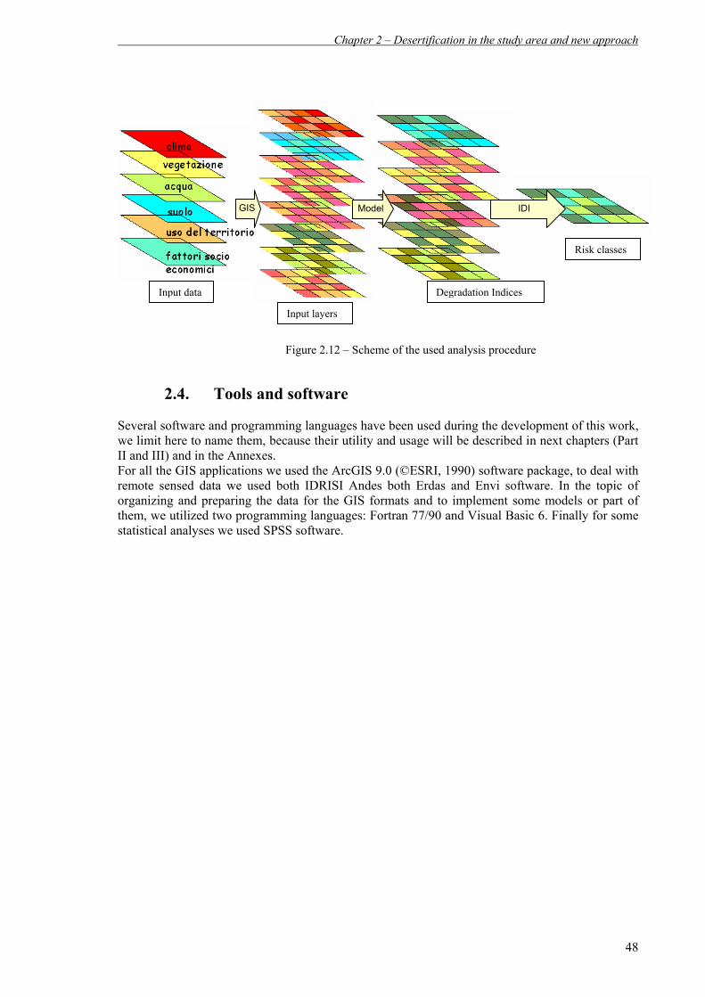
Chapter 2 – Desertification in the study area and new approach
48
Figure 2.12 – Scheme of the used analysis procedure
2.4. Tools and software Several software and programming languages have been used during the development of this work, we limit here to name them, because their utility and usage will be described in next chapters (Part II and III) and in the Annexes. For all the GIS applications we used the ArcGIS 9.0 (©ESRI, 1990) software package, to deal with remote sensed data we used both IDRISI Andes both Erdas and Envi software. In the topic of organizing and preparing the data for the GIS formats and to implement some models or part of them, we utilized two programming languages: Fortran 77/90 and Visual Basic 6. Finally for some statistical analyses we used SPSS software.
GIS Model IDI
Risk classes
Degradation Indices Input data
Input layers

PART II
Chapter 3 – The water erosion assessment model - RUSLE
50
3. The water erosion assessment model - RUSLE
3.1. Introduction
The water erosion refers to the removal of soil because of rain impact, runoff and gravity, and it is due to water under different forms: direct rain, ice-snow melting, irrigation water, rivers. But the main factor is the rain, according to drop dimensions, the angle and velocity of impact and if during the rain event there are winds or not. The main process is the running of water on the soil surface, but also the diminution of the infiltration rate, as the rain makes the soil more and more saturated and no longer capable to absorb water, causing the increasing of superficial runoff. The phenomenon is however linked to topography (slope, that influence the water velocity), to aspect of hill-slopes (influencing the soil moisture), to vegetation cover (that protects the soil), to soil structure (the presence or absence of aggregates) and to practices for cultivating and protecting soil by erosion. This process of water erosion is certainly one of the dominant degradation processes on the North of Mediterranean area and it can lead to a loss of soil often irreversible. Sardinia island is a region with a dry climate where the scarcity of water creates problems every day. Nevertheless, the rain events, often with a torrential nature, are a negative episode rather than an event mitigating the aridity. Indeed the soils are highly erodible as principally dried by interaction of sun/wind. This happens in particular over the most elevated areas where the combination of precipitation amount and steep slope can easily generate runoff through wide areas: this can create strong problems also along transport lines (e.g. the case of Foxi’s area, along the highway Cagliari-Nuoro). It starts from here the necessity to evaluate the erosion risk as help to decision support system against desertification, with the aim to carry out rational intervention and mitigation measures, both at local and at regional scale, allowing to limit the total quantity of soil loss.
3.2. Description of the model
The technology for predicting erosion consists in mathematic equations calculating the eroded quantity using as input variables the ones related to soil, to climate, to topography and to land use. Numerous formulas estimate the soil loss given by erosion, transport and deposition by water but, despite the large quantity of available models to evaluate the erosion vulnerability and risk, most of them require such a complex and different input data that for an application at small scale it becomes a complicated challenge. The RUSLE (Revised Universal Soil Loss Equation, Renard et al., 1997) is an empirical model very easy in its formulation, where to each variable influencing the erosion it is associated an index representing the effect of that variable over the erosion itself according to the value assigned to that index. To estimate soil loss, the RUSLE equation is the most used as it can be applied in different situations, also with very complex topographies, and it is largely supported by GIS tools, in order to fast obtain erosion susceptibility maps. Moreover it has often been used at different spatial scales and it is one of the models requiring less input data, easy to acquire or to derive and it allows to make appropriate choices according to the extension of the study area, the availability of data and the objectives of the study. The soil loss is calculated in our study by RUSLE as “quantity of lost sediment per unit of surface”, using following equation: A= R*K*LS*C*P (3.1)

Chapter 3 – The water erosion assessment model - RUSLE
51
where A is the output, that is the annual loss of soil for rill/sheet erosion (t/(ha*year)) R is the rain erosivity factor (MJ·mm·ha-1·h-1·y-1) K is the soil erodibility factor (T·h / MJ·mm) LS is the combined topographic slope-length and slope steepness factor (unitless) C is the vegetation cover factor (unitless) P is the factor related to practices for erosion reduction (support practice factor) (unitless)
Each of above listed factors of RUSLE can assume values representing the best conditions (lower values) or the worst conditions (higher values). In the following these factors will be analyzed with more detail (par. 3.3), describing the steps in deriving them after elaborating the ancillary data (par 3.4) and before running the model. It is important to highlight that despite a lot of literature and scientific documentation available for this model, there was not a source-code available and already implemented into GIS environment, consequently the model was completely re-written, adapting the reading of inputs, the computation and the output creation to the requests of GIS visualization and processing software used in the project. The programming language to implement RUSLE was FORTRAN 90/95, with the result of an executable file RUSLEs.exe, where “RUSLE” is the model name and “s” stands for Sardinia.
3.3. Parameterization and modifications to the model
3.3.1. R factor: rain erosivity
As already said, rain is the acting force in the water erosion process; both because of rain impact that detaches particles of soil both for runoff that transports those detaching further particles. To calculate rain erosivity index R (MJ·mm·ha-1·h-1·y-1) of RUSLE according to the official formulation in eq. 3.1, it is necessary to operate, for each single rain event within the interval of years of interest, the half-hour precipitation amounts (mm) and the maximum peak of precipitation intensity (mm/h) with kinetic energy of rain (E), in order to calculate the energy of the event itself (EI30). The formula to calculate erosivity considers the product of the storm’s energy and its maximum 30-minute intensity (for an individual storm) is (Wischmeier and Smith, 1978):
30EIRs = (3.2) where: Rs = storm erosivity (MJ*mm / (ha*h)), E = storm energy (MJ/ha), and I30 = maximum 30-minute intensity (mm/h). I30 is the average intensity over the continuous 30 minutes in the storm with the most rainfall. Storm energy is computed using (Renard et al., 1997):
k
m
kk PeE ∆= ∑
=1 (3.3)
where: e = unit energy [MJ/(mm·ha)] (energy content per unit area per unit rainfall depth) in the kth period, ∆P = the depth of rainfall (mm) in the kth period, and m = the number of periods of 30 minutes in the rainstorm. Unit energy is computed from (Brown and Foster, 1987; Renard et al., 1997):
[ ])082.0exp(72.0129.0 kk ie −−= (3.4) where ik = rainfall intensity (mm/h) for the kth period. The combined formula for the ensemble of events is:

Chapter 3 – The water erosion assessment model - RUSLE
52
(3.5) Where i indicate the single event and n the number of events. But, because of the lack in Sardinia of available meteorological data with the necessary temporal interval of acquisition (half-hour), we decided to calculate the R factor by the Arnoldus (1980) method and by the Fournier (1960) index, largely used in literature and with an adequate validation support. Indeed, a modified Fournier index is widely used to estimate erosivity where precipitation data with the needed interval are very limited. A value for the modified Fournier index, based on using annual and monthly precipitation amount values, is computed from (Renard and Freimund, 1994):
15217.4 −= FR (3.8)
where F is the Fournier index given by:
P
PiF i
∑==
12
1
2
(3.9)
with Pi = mean precipitation of the ith month (mm) P = mean annual precipitation (mm) and i varying from 1 to 12.
3.3.2. K factor: soil erodibility
The soil erodibility factor (T·h / MJ·mm) represents the attitude of soil to be eroded according to its physical and chemical properties, in particular according to following soil attributes: 1. texture (percent content of sand, silt and clay); 2. organic matter content; 3. drainage capacity; 4. soil structure. The equation for the standard soil erodibility nomograph (Wischmeier and Smith, 1978; Renard et al., 1997) is:
( )[ ]4.759
psot kkkkK
++⋅= (3.10)
where: K = soil erodibility factor
kt = texture subfactor ko = organic matter subfactor ks= soil structure subfactor, kp =soil profile permeability subfactor.
About the first component kt, the soil texture subfactor equation is given by (Wischmeier et al., 1971):
( )( )( )∑ ∑= =
⎟⎠
⎞⎜⎝
⎛∆⋅⋅−⋅⋅∆⋅=
n
i
m
kkk PPIR
k1 1
30 2082.0exp72.0129.0

Chapter 3 – The water erosion assessment model - RUSLE
53
( )( )[ ] 100001001.2 14.1clvfssltb PPPk −+= (3.11)
tbt kk = (3.12) where: Psl = percent of silt, Pvfs = percent of very fine sand based on the total soil primary particles and not just the portion of the sand content, and Pcl = percent of clay. Although eq. 3.11 was derived using regression analysis, Wischmeier et al. (1971) used judgment to graphically draw the kt relationship for Psl + Pvfs percentage above 68%. The equations fitted to the Wischmeier et al. (1971) graphical curves is:
( )[ ] 10000100681.2 14.1cltb Pk −= (3.14)
( )[ ]82.06867.0 ttbtbt kkkk −−= (3.15)
About the second component ko, the equation for the soil erodibility nomograph organic matter sub-factor is:
mo Ok −= 12 (3.16) where: Om = percent of soil organic matter contained in the soil. About the third component kp, the soil permeability subfactor is a measure of the potential of the soil profile for generating runoff. Six permeability classes that range from 1-rapid (very low runoff potential) to 6-very slow (very high runoff potential) are used to rate the soil profile for infiltrating precipitation and reducing runoff. The equation for the permeability subfactor is given by:
( )35.2 −= tp Pk (3.17) where: Pt = the soil profile permeability rating. About the fourth component ks, the soil structure subfactor refers to how the arrangements of soil primary particles in aggregates and the arrangement of aggregates in the soil affect erosion. Four structural classes are used in the nomograph: 1-very fine granular; 2-fine granular; 3-medium or coarse granular; 4-blocky, platy, or massive. These classes are defined in the USDA-NRCS soil survey manual (USDA-NRCS, 1993). The equation for the soil structure subfactor is:
( )225.3 −= ss Sk if ( ) 7≥+ sot kkk (3.18) 7=+ sot kkk if ( ) 7<+ sot kkk (3.19)
where: Ss = the soil structure class. After calculating kp, ks, kt, ko the K factor into RUSLE model could be derived choosing between two following equations: 1) (Wischmeier e Smith, 1978)

Chapter 3 – The water erosion assessment model - RUSLE
54
[ ][ ][ ]210 7101.0/)659.1(log5.00405.00034.0594.7 +−⋅+= gDeK (3.20)
considering only the textural classes, where Dg (mm) is the mean geometric diameter of particles, given by:
)ln01.0( ∑= i
ii mf
eDg (3.21) with fi = textural fraction of sand, silt, clay classes (i) mi = geometric mean of particle diameter comprised into the ith class, and it is equal 316.2 µm for sand, 10 µm for silt, 0.3162 µm for clay. 2) (Renard, 1997)
( )[ ]4.759
psto kkkkK
++⋅= (3.22)
This formula considers all the four coefficients previously calculated. As example, the erodibility degree of soil can be classified according to the following Table 3.1 (Simms et al., 2003).
Table 3.1 – Classes of erodibility according to the range of values of K factor
3.3.3. LS factor: topography
The topographic factor has the role of describing how topography influences the erosion processes. It is based on length and steepness of slope, regardless of land use. According to Foster & Wischmeier (1974) the topographic factor for irregular slopes is:
( )( )∑= −
+−
+
−
−⋅=
N
jm
jj
mjj
mjj SS
LS1 1
11
1
13.22λλ
λλ (3.23)
where Sj = slope factor for jth segment (m/m) along the path of the slope, λj = distance from the lower boundary of the jth segment to the upslope field boundary (m), m = slope length exponent Eq. 3.23 can be expanded for a three-dimensional topography:

Chapter 3 – The water erosion assessment model - RUSLE
55
( ) ( ) ( ) ( )( ) ( )( ) ( )∑
⋅−
⋅−⋅=
++
jim
inletoutlet
minlet
moutlet
jijijijiSjijiS
LS,
11
13.22,,,,,,
λλλλ
(3.24)
Where, in this case LS = topographic factor within the RUSLE for a parcel or the whole catchment (see below)
is the summation for all grid cells within the parcel or the whole catchment
λ(i,j)inlet = slope length at the inlet of grid cell (i,j) (m) λ(i,j)outlet = slope length for the outlet of grid cell (i,j) (m) S(i,j) = slope factor for grid cell (i,j) m = slope length exponent (see later) For two-dimensional applications, we have to replace slope length by “unit contributing area”. The unit contributing area can be defined as the contributing area per unit of width. To calculate the unit contributing area we have to divide the contributing area by the width over which flow can pass within a grid cell. This width depends on the flow direction and is calculated using the aspect direction (Desmet & Govers, 1996). This means: λ(i,j)inlet = As,in = Ain/D' λ(i,j)outlet = As,out = Aout/D' where As,in = unit contributing area at the inlet of the grid cell, As,out = unit contributing area at the outlet of the grid cell, D' = width over which flow can pass within the grid cell. with Aout = Ain + D’2 and D’ = D/x where D = grid spacing and x = correction factor equal to 1 if the direction toward the outlet cell is a cardinal direction, and the square root of 2 if the direction toward the outlet cell is a diagonal direction.
( ) ( )( ) ( )m
inin
min
min
mm ADAADA
DD
xxjiL
13.22,
2
112
11 ⋅−+
−+=
++
++ (3.25)
( ) ( )( ) ( )( )mmm
mm
DxjiADjiAjiL
13.22,,,
2
112
⋅⋅−+
=+
++
(3.26)
The m exponent was evaluated in the following way: = 0.5 if the slope toward the considered direction is ≥ 0.05 = 0.4 if the slope toward the considered direction is ≥ 0.035 and < 0.05 = 0.3 if the slope toward the considered direction is ≥ 0.01 and < 0.035 = 0.2 if the slope toward the considered direction is < 0.01
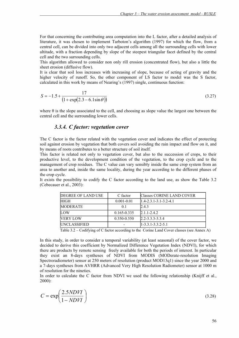
Chapter 3 – The water erosion assessment model - RUSLE
56
For that concerning the contributing area computation into the L factor, after a detailed analysis of literature, it was chosen to implement Tarboton’s algorithm (1997) for which the flow, from a central cell, can be divided into only two adjacent cells among all the surrounding cells with lower altitude, with a fraction depending by slope of the steepest triangular facet defined by the central cell and the two surrounding cells. This algorithm allowed to consider non only rill erosion (concentrated flow), but also a little the sheet erosion (diffusive flow). It is clear that soil loss increases with increasing of slope, because of acting of gravity and the higher velocity of runoff. So, the other component of LS factor to model was the S factor, calculated in this work by means of Nearing’s (1997) single, continuous function:
( )( )θsin1.63.2exp1175.1−+
+−=S (3.27)
where θ is the slope associated to the cell, and choosing as slope value the largest one between the central cell and the surrounding lower cells.
3.3.4. C factor: vegetation cover
The C factor is the factor related with the vegetation cover and indicates the effect of protecting soil against erosion by vegetation that both covers soil avoiding the rain impact and flow on it, and by means of roots contributes to a better structure of soil itself. This factor is related not only to vegetation cover, but also to the succession of crops, to their productive level, to the development condition of the vegetation, to the crop cycle and to the management of crop residues. The C value can vary sensibly inside the same crop system from an area to another and, inside the same locality, during the year according to the different phases of the crop cycle. It exists the possibility to codify the C factor according to the land use, as show the Table 3.2 (Cebecauer et al., 2003):
DEGREE OF LAND USE C factor Classes CORINE LAND COVER HIGH 0.001-0.01 1.4-2.3.1-3.1-3.2-4.1 MODERATE 0.1 2.4.3 LOW 0.165-0.335 2.1.1-2.4.2 VERY LOW 0.350-0.550 2.2-3.3.3-3.3.4 UNCLASSIFIED - 1-3.3.1-3.3.2-5.1 Table 3.2 – Codifying of C factor according to the Corine Land Cover classes (see Annex A)
In this study, in order to consider a temporal variability (at least seasonal) of the cover factor, we decided to derive this coefficient by Normalized Difference Vegetation Index (NDVI), for which there are products by remote sensing freely available for both the periods of interest. In particular they exist an 8-days syntheses of NDVI from MODIS (MODerate-resolution Imaging Spectroradiometer) sensor at 250 meters of resolution (product MOD13q1) since the year 2000 and a 7-days syntheses from AVHRR (Advanced Very High Resolution Radiometer) sensor at 1000 m of resolution for the nineties. In order to calculate the C factor from NDVI we used the following relationship (Knijff et al., 2000):
⎟⎠⎞
⎜⎝⎛−
=NDVINDVIC
15.2exp (3.28)

Chapter 3 – The water erosion assessment model - RUSLE
57
For that concerning the remote sensed NDVI, we had to make a downscaling to make these at 50 meters of resolution, for both the reference periods. For the MODIS sensor data, this has been done considering the Corine Land Cover Map relative to the year 2003 and at scale 1:25000 (Annex A). For early nineties period we started from another resolution, the 1000 m of the AVHRR sensor, to derive NDVI map at 50 meter of resolution, and we used the Corine Land Cover Map relative to the year 1990 and at scale 1:100’000 (Annex A). The downscaling methodologies used are described in detail at the end of the thesis (Annex C and D).
3.3.5. P factor: management practices against erosion
The P factor indicates the anti-erosive effect given by some actions made for soil protection or by all that can be an obstacle to erosion: i.e. installation of practices that slow runoff and thus reduce soil movement. In general, the principal countermeasures used to limit erosive effects are the ploughing/tilling according to the contour lines of elevation (transversal tillage), the arrangement of soil in strips, the arrangement with terraces and working the lands a rittochino. Given the extent of the area and the impossibility to have detailed information for each part of the region about the type of land arrangement/working, and given the lack of complete look up tables to associate to a certain type of land use an adequate P factor value, we decided to integrate the P factor inside the LS factor (that, we remember, if alone doesn’t consider the land use). The reason was that the limitation and reduction of area contributing to the flow (contributing area) is the main component over which the practices to reduce erosion can act. In this work, P factor was evaluated considering that there are areas not generating flow (non erodible areas) and/or stopping the flow itself (breaklines). This two types of areas have been inserted into the LS factor, determining a stop in the increase of contributing area computation and a zeroing of the contributing area where these breaklines occur. These areas are for example the boundaries among different land use type (where there are often furrows to drain overland flow of water), the roads and the railway lines (whose border have often bump) and rivers (whose borders have often banks). This integration between the two factors, P and LS, will also allow for example to consider the effects of probable protection works inside a given type of land use (e.g. ditch to water drainage) required by Good Agricultural Practice.
3.4. Production and format of input data
The model was written in order to deal with one of the most common GIS formats, the ASCII grid format (an ESRI owner format), which is easily importable into the GIS environment of different software (ArcGIS, IDRISI etc.). The grid is a text file that contains all values of the individual grids, presenting the values for separate cells. In this format the values for the individual cells are stored in rows and columns with a header that describes the format. All the input data of the model are in ASCII grid format and present the same characteristics of extent relative to:
1. Number of columns; 2. Number of rows; 3. X coordinate of the lower left corner; 4. Y coordinate of the upper left corner; 5. Dimension of the cell 6. No data (invalid) values (in our case always -9999)
It is not possible for the model to manage, indeed, inputs with one or more of above listed characteristics different from one to another. In order to set and standardize all the inputs, we predisposed a reference “work-mask” applied at the entire input data production chain (Figure 3.1)

Chapter 3 – The water erosion assessment model - RUSLE
58
Moreover, it was necessary the perfect spatial correspondence of cell borders and of no data distribution.
Figure 3.1 – Work mask
We list in the following the input data required to implement the model, their units of measure, their necessary time step and their format. In particular five datasets have been at the basis of derivation of inputs for the RUSLE model: the Corine Land Cover Database (for the years 1990 and 2003), the Pedologic Map of Sardinia, produced specifically for the project, the Digital Elevation Model (DEM), the remote sensed NDVI and the climatic data. The detailed description of these datasets is contained into the Annex A, but here we want to remember that for some inputs (Corine Land Cover, NDVI and climate) the processing operations described in the following have been done for two sets of data, the former relative to early nineties period and the latter relative to the actual period, as we will explain into the specific paragraphs.
3.4.1. Erodible areas We stated to consider for running of the model only the really erodible parts of the territory. To do this we reclassified the field regarding the texture of the Pedologic map according to following Table 3.3:
Class Value Coarse 1 Medium 2 Medium fine 3 Fine 4 Very fine 5 Other 6
Table 3.3 - Texture codifying The code 6 (“other”) indicates all that is non-erodible: the wet and urban areas in the Pedologic Map that is areas where there is not an erosive process because of the lack of soil. To improve the detail of this input data, we continued codifying as “other” also areas corresponding to specific classes of Corine Land Cover (for the legend we refer also to Annex A), that is:
a) CORINE 1990: Classes 1, 4, 5, 2111 (nursery and protected cultivation) and 332 (Bare rocks and cliff)
b) CORINE 2003: Classes 1, 4, 5, 2123 (nursery), 2124 (greenhouse cultivation), 3315 (river beds larger than 25 meters) e 332 (Bare rocks and cliff)
This input from original vector format of Pedologic Map was converted in grid layer.

Chapter 3 – The water erosion assessment model - RUSLE
59
3.4.2. R factor
As already said, the amount of monthly precipitation gives us an indication of the strength of erosive agent (rain) and it is directly used by the model to calculate, by means of Arnoldus (1980) formula, the R factor. The monthly precipitation data have been obtained by summing daily precipitation maps at 1 km of resolution, supplied by Laboratorio di Simulazioni Numeriche del Clima e degli Ecosistemi Marini (University of Bologna, Italy) and produced by spatializing the station data (for a maximum of 18 regional stations comprising the UCEA station and the NOAA stations, see Annex A) taking into account also relationships among climatic variables and topography, for the interpolation was used a krigging function. Following Figure 3.2 illustrates the methodology.
Figure 3.2 – Scheme showing the main operation made over the precipitation data: spatilization (interpolation) of station data into grids. In particular, in order to work with a mean climatic year and not with a single year that could be not representative, we averaged the monthly precipitation of five years for the early nineties (1991-1992-1993-1994-1995), and of five years representing actual period (2001-2002-2003-2004-2005). Monthly data were then ready to the input of model, in total we produced 24 grids, 12 monthly grids for each period of reference. Given the typical precipitation regime of the region, only in one case and in one restricted area, with a precipitation amount very low, R index resulted negative: in this case it was set to 0.
Station Precipitation Data non spatialized
Input formato ASCII
INTERPOLATION

Chapter 3 – The water erosion assessment model - RUSLE
60
3.4.3. K factor ko
The organic matter content was derived by a field of Pedologic Map of Sardinia presenting five codes for each class: 1) low, 2) medium, 3) high, 4) very high and 5) other and corresponding to ranges of percent content to which we associated the mean representative value (Table 3.4).
Table 3.4 - Codifying of soil organic matter content
This extracted representative values (Om) for each class of organic matter content were operated in the eq. 3.16 to derive the organic matter content coefficient ko. With “other” we indicated the wet and urban areas in the Pedologic Map. This input from vector format of Pedologic Map was converted in grid layer . kt
As already said the kt coefficient of K factor requires three inputs: clay content (particles smaller than 0.064 mm), silt content (particles between 0.064 mm and 2 mm) and sand content (particles larger than 2 mm), all in fraction (not percent). We distinguished five textural classes (coarse, medium, medium-fine, fine, very fine) according to the textural triangle of Figure 3.3 that, starting by percent composition of sand, silt and clay, allowed to reclassifying the field of the texture of the Pedologic Map according to Table 3.5:
Figure 3.3 – Textural composition of the five classes considered in model parameterization
Class Clay Silt Sand Coarse 0.079 0.136 0.786 Medium 0.176 0.404 0.420 Medium fine 0.170 0.760 0.070 Fine 0.460 0.270 0.270 Very fine 0.733 0.133 0.133 Other 0 0 0
Table 3.5 - Codifying of the sand, silt, clay content of soil With “other” we indicated wet and urban areas in the Pedologic Map. These input data from vector format of Pedologic Map were converted in three grid layers.
Class Code Content(%) Representative Percent Low 1 > 6 and < 12 9%
Medium 2 > 2 and ≤ 6 4% High 3 > 1and ≤ 2 1.5%
Very High 4 ≤ 1 0.5% Other 5 - -
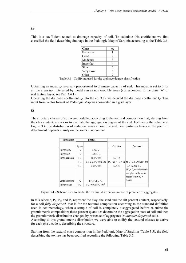
Chapter 3 – The water erosion assessment model - RUSLE
61
kp
This is a coefficient related to drainage capacity of soil. To calculate this coefficient we first classified the field describing drainage in the Pedologic Map of Sardinia according to the Table 3.6.
Class cd Eccessive 1 Good 2 Moderate 3 Imperfect 4 Slow 5 Very slow 6 Other 7
Table 3.6 - Codifying used for the drainage degree classification Obtaining an index cd inversely proportional to drainage capacity of soil. This index is set to 0 for all the areas non interested by model run as non erodible areas (correspondent to the class “6” of soil texture layer, see Par. 3.4.1). Operating the drainage coefficient cd into the eq. 3.17 we derived the drainage coefficient kd. This input from vector format of Pedologic Map was converted in a grid layer. ks
The structure classes of soil were modelled according to the textural composition that, starting from the clay content, allows us to evaluate the aggregation degree of the soil. Following the scheme in Figure 3.4, the distribution of sediment mass among the sediment particle classes at the point of detachment depends mainly on the soil’s clay content:
Figure 3.4 – Scheme used to model the textural distribution in case of presence of aggregates.
In this scheme, Pcl, Psa and Psl represent the clay, the sand and the silt percent content, respectively, for a soil fully dispersed, that is for the textural composition according to the standard definition used in sedimentology, when a sample of soil is completely disaggregated before calculate the granulometric composition; these percent quantities determine the aggregation state of soil and then the granulometric distribution changed by presence of aggregates (minimally dispersed soil). According to this granulometric distribution we were able to codify the textural classes to derive for each one a code cs describing the structure. Starting from the textural class composition in the Pedologic Map of Sardinia (Table 3.5), the field describing the texture has been codified according the following Table 3.7:
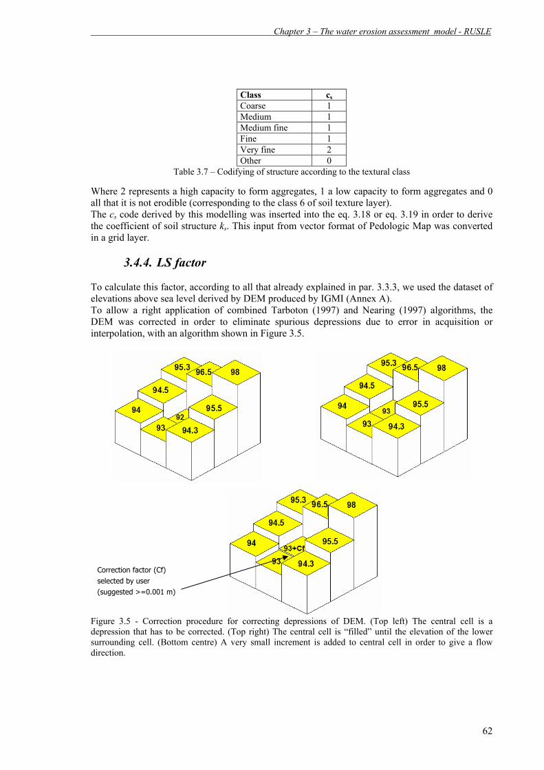
Chapter 3 – The water erosion assessment model - RUSLE
62
Class cs Coarse 1 Medium 1 Medium fine 1 Fine 1 Very fine 2 Other 0
Table 3.7 – Codifying of structure according to the textural class
Where 2 represents a high capacity to form aggregates, 1 a low capacity to form aggregates and 0 all that it is not erodible (corresponding to the class 6 of soil texture layer). The cs code derived by this modelling was inserted into the eq. 3.18 or eq. 3.19 in order to derive the coefficient of soil structure ks. This input from vector format of Pedologic Map was converted in a grid layer.
3.4.4. LS factor
To calculate this factor, according to all that already explained in par. 3.3.3, we used the dataset of elevations above sea level derived by DEM produced by IGMI (Annex A). To allow a right application of combined Tarboton (1997) and Nearing (1997) algorithms, the DEM was corrected in order to eliminate spurious depressions due to error in acquisition or interpolation, with an algorithm shown in Figure 3.5.
Figure 3.5 - Correction procedure for correcting depressions of DEM. (Top left) The central cell is a depression that has to be corrected. (Top right) The central cell is “filled” until the elevation of the lower surrounding cell. (Bottom centre) A very small increment is added to central cell in order to give a flow direction.
Correction factor (Cf) selected by user (suggested >=0.001 m)

Chapter 3 – The water erosion assessment model - RUSLE
63
3.4.5. P factor
According to all that explained in par. 3.3.5 we chose to model the practices to reduce erosion inside the LS factor, so we created a dichotomic map containing 1 for all those positions where there was not an interruption of flow, and 0 where there are features (roads, railways, river, land use boundaries) that sometimes constitute an obstacle to flow and then stop or reduce it producing a zeroing of upslope contributing area. So, this P factor was produced crossing and joining information coming from following informatic layers (Annex A): • Corine Land Cover • Pedologic Map of Sardinia • Hydrographic map • Road network map • Railway network map In practice, we rasterized the hydrographic network, the road network and the railway network vector layers giving 0 to all these elements. Then we rasterized the boundaries of different patches of land use map (Corine Land Cover) to the third level of classification, giving them the value 0 (Figure 3.6).
Figure 3.6 – Selection of features that have been converted into areas stopping the water flow
Finally we rasterized the urban areas and the wet areas polygons of Pedologic Map giving them a no data values, as in these areas there is no erosion or flow. Moreover, we gave no data values to all the Corine Land Cover classes for which the erosive process is null, that is:
c) CORINE 1990: Classes 1, 4, 5, 2111 (nursery and protected cultivation) and 332 (Bare rocks and cliff)
d) CORINE 2003: Classes 1, 4, 5, 2123 (nursery), 2124 (greenhouse cultivation), 3315 (river beds lager than 25 meters) e 332 (Bare rocks and cliff)
All these information were merged into a single grid.
Urban
Patch boundaries
Corine Land Cover Road, river and railway network

Chapter 3 – The water erosion assessment model - RUSLE
64
3.4.6. C factor
The NDVI data, useful for reconstructing the temporal variation of C factor, were obtained for the periods of interest by MODIS sensor (year 2003, Annex A), and by AVHRR sensor (year 1995, Annex A), according to the large availability of data and the best quality of images. First of all, as there were many images with numerous invalid values both for cloud problems and because of sensor errors, we carried out the gap-filling of images to recover data using a methodology that for a given invalid pixel of an image make a mean between the previous and the next images (Annex B). Then we made a downscaling to 50 meters of resolution, considering for both periods the land use map by Corine Land Cover dataset (Annex C). In order to derive NDVI data for the year 1995 comparable with the NDVI relative to the year 2003, we first calculated the relationships between the AVHRR NDVI at 1 km of resolution and the MODIS NDVI at 1 km of resolution, comparing the images regarding the same date interval for the year 2003 (Figure 3.7), and working on a land use basis (third level of the Corine Land Cover database). Then we calculated a “synthetic” MODIS NDVI for 1995, by inverting the found relationship with the AVHRR NDVI for the year 1995. This layer was downscaled first at 250 meter of resolution considering the land use map for the year 1990, then it has been re-sampled at 50 meters of resolution (Annexes C and D).
Figure 3.7 – The image shows an example of regression between the NDVI-MODIS (modis_ndvi2003161) and the NDVI-AVHRR (w20030609) images at 1 km of resolution (date: 9 june 2003), used to reconstruct the NDVI values for the year 1995 starting from the AVHRR NDVI for the year 1995, comparable with MODIS NDVI. Then from this set of NDVI images we calculated four seasonal averages at 50 meters of resolution, and these data have been corrected for the missed data by using statistical analyses. Indeed the areas characterized by no_data because of lack of values in the original images, were treated carrying out a zonal statistics between MODIS datum and Corine Land Cover: for each land use class (considered at the third level of classification), we calculated the mean value of NDVI, then this value was assigned to no_data areas present in the image according to the land use class (Figure 3.8).

Chapter 3 – The water erosion assessment model - RUSLE
65
Figure 3.8 - Zonal statistics: The mean values of NDVI calculated for each type of land use (level III of the Corine Land Cover database), were used to substitute no_data occurring in the original MODIS image. Finally we masked the areas corresponding to the code 6 of the soil texture layer, where we already decided the model had not to run.
3.4.7. Other input data Further, besides spatialized data, we needed an input file for our model, input_rusle.txt containing 14 rows with the following information: 1st row: year of simulation (4 digits, i.e. 2003 for the year 2003) 2nd-13th rows: month of simulation (2 digits, from 01 to 12) 14th row: method to calculate K factor: 1=Wischmeier and Smith (1978), 2=Renard (1997) Finally the file soil_grid_files.txt (Figure 3.9) contains the list of all the grids relative to surface/soil data, excluding the climatic ones.
NoData in the MODIS image
Mean NDVI values calculated by zonal statistic according to the land use class
Substitution of NoData with mean NDVI calculated on a land use basis

Chapter 3 – The water erosion assessment model - RUSLE
66
Figure 3.9 – Content of the file soil_grid_files.txt
3.5. SIMULATION AND RESULT DISCUSSION
Two simulations were made using the RUSLE model, the former with a set of data relative to early nineties period (the chosen range of years was 1991-1995), the latter with a set of data relative to most recent situation (reference years 2001-2005). The model spent about 90 minutes in each run for the entire regional territory, in both case the output was a grid, representing the soil loss in t/ha*year. We show in the following (Figure 3.10) the maps result of simulation that afterwards will be operated into the IDI. It is clear that, together with an increase of the total annual amount of precipitation for the period 2001-2005 as respect the period 1991-1995, there was a diffuse increase of erosion quantities, that we can notice also by maximum values of the scales, that in the most recent period is double than the past period. Figure 3.10 - The images show the RUSLE results for the two reference periods, 1991-1995 (left) and 2001-2005 (right). The values in legend are t/(ha*year) As in the two periods the other inputs are somewhat “static”, the model was sensible to climatic inputs that determine the strength of the erosive acting. On speaking about the increase of precipitation, we have to specify that the tendency is an diminution of their frequency but an

Chapter 3 – The water erosion assessment model - RUSLE
67
augment of their intensity. Indeed in last decades we assisted to a more and more marked alternation of long drought periods (when the soil is subjected to drying and to fracture creation) and rare rainy periods, with brief precipitation episodes but intense and torrential. In this way the soil is soon incapable to infiltrate water in the subsoil, causing an augment of runoff and of solid transport. Looking at the spatial distribution of steepest slopes and low vegetation covers, we notice that the model was sensible also to these inputs. Considering in particular the simulation about the most recent period, we can individuate three “hotspots” of erosion: an area of the Gennargentu chain, an area directly to North-East of the Campidano’s depression and the last one to the south-east borders of the Nurra area. Analyzing the distribution of differences between the two periods of reference, it seems that the positive differences (that is erosion larger in the recent period as respects the past one) are distributed over the bare areas with an agricultural use (Campidano area and Sassari province area), all that confirm the sensibility of the model to vegetation cover and in particular to its seasonal variability. In the next Figure 3.11 to the left we can see the distribution of the main land use classes, to the right the differences in erosion quantity between the two reference periods.
Figure 3.11 – Map of reclassified land use (left) and map of the differences in erosion between the recent period and the past one (right: red areas = positive difference; blue areas = negative difference) Deeply and spatially analyzing the model results and their occurring according to the land use, we noticed the necessity to find a way for masking the model output of some areas like bare rocks,

Chapter 3 – The water erosion assessment model - RUSLE
68
very steep areas (quasi vertical walls), sparsely or not vegetated lands, for which we cannot speak of desertification phenomena, but of areas “naturally desertified”. First we individuated those areas whose RUSLE results were equal or larger than 30t/ha*year. Indeed these areas represent part of the territory where we can have a wrong perception of the desertification because their conditions are not linked to the phenomenon (these values are outliers of value distribution). Then we extracted the areas with sparse or no vegetation, that is the 333, 3241, 3242 Corine Land Cover classes. Finally we extracted the areas with a slope greater than 25%. The final mask was obtained combining the areas where all of the three above described characteristics occurred. In the next Figure 3.12 we can see an example of the output of the methodology to mask area “naturally desertified”, over which to carry out a smoothing of the RUSLE values.
Figure 3.12: Overlay of three extreme situations considered in extracting the mask with the areas to consider “naturally desertified” and where to apply a smoothing of the RUSLE model output: blue areas are the ones with a RUSLE result larger than 30 t/ha*y, red areas are the masked CORINE classes, green areas are the ones with a slope larger than 25%. Finally, black areas are the ones where previous conditions combine together.
Inside the masked areas we applied an inverse stretching algorithm from 0 to 90% to calibrate RUSLE value. In the following Figures 3.13 and 3.14 it is shown the calibration result. As we can see, without the smoothing the range of values is significantly wider.

Chapter 3 – The water erosion assessment model - RUSLE
69
Figure 3.13: Output of the RUSLE model without calibration
Figure 3.14: Output of the RUSLE model with calibration
Then, to calibrate RUSLE model, we have not carried out new runs, but we applied a posteriori a smoothing procedure, before to put the index in the IDI formula.

Chapter 3 – The water erosion assessment model - RUSLE
70
In validating model results we considered several works carried out to measure the runoff and the erosion under different land use (e.g. Vacca et. al, 2000). A detailed study concerns for example the Santa Lucia’s river basin, on the south of island, where they were carried out experiments about erosion in the period 1992-1997, giving mean values of erosion for different land use ranging from 0.8 to 1 t/ha*year: making a mean over the same basin of erosion values estimated by our application of RUSLE, we obtained a quantity of 1.3 t/ha*y, that is the same order of magnitude. Further, experimental data taken by the ISSDS (Istituto Sperimentale per lo Studio e la Difesa del Suolo) database and regarding several (44) Italian lakes and rivers, we extracted the typical values of erosion for two sub-basins called Mulargia and Flumendosa (whose location is reported in Figure 3.15), having together a mean value of erosion of 5.56 t/ha*year. A zonal statistic over these two basins that, in our database, are comprised into the larger basin simply called basin of Flumendosa gave us a result of about 6.5 t/ha*year.
Figure 3.15 - Location of the two sub-basins of the Flumendosa basin for which they exists data of erosion (t/ha*year) in the ISSDS database. Anyway, as already said in Chapter 2, to associate to each erosion quantity a degradation index, we had to normalize the resulted quantities for a value considered critical. To normalize we chosen to consider the local reality and, in order to avoid underestimation of local criticality, do not consider an absolute value retained critic for erosion. The standardization procedure is explained in Chapter 9, as the methodology of post-processing over model results has been implemented directly into the IDI tool.

Chapter 4 – The overgrazing assessment model - CAIA
71
4. The overgrazing assessment model - CAIA
4.1. Introduction
The irrational practice of stock raising (Yassoglou, 1999) is considered one of the most important factors of soil degradation in arid and semiarid regions and it is evident in some regions with an arid climate (Greek islands, Sardinia and Sicily in Italy, southern Spain, Morocco). In these areas the breeding, jointly with fire employment for pastureland cleaning and preparation, caused in the past a strong reduction of soil fertility (Pulina et al., 1997). The cattle/sheep breeding is the main branch of Mediterranean agricultural activities, in this region, indeed, it is estimated there are more than one hundred millions of heads of cattle. Sardinia is one of the Italian regions where the anthropogenic pressure due to sheep farming provokes diffuse degradation phenomena (Rivoira et al., 1997). According to the most recent information, on a regional territory of 24’089 km2, about the 80% consists in agricultural areas with about 762’800 heads, of which the 56% are sheep used for milk production (D’Angelo et al., 2000). At this time in Sardinia the lands devoted to pasture are not enough to meet the needs of animals: for example, while the forage production is concentrated in spring, the energetic requirements of sheep are in autumn and winter. In the past this was resolved by transhumance (Enne et al., 1998), but in the last 40 years there was an intensification of grazing in the hilly areas, causing a modification of the landscape and an increase of degradation/desertification phenomena. Establishing a set of indicators useful in evaluating the impact of overgrazing on desertification is a very difficult challenge, as the agro-pastoral systems are very variable in space and in time.
4.2. Description of the model The evaluation of the grazing intensity was made by means of the model CAIA (Carico Animale di Impatto Ambientale –Environmental Impact Grazing Pressure) (Pulina e Zucca, 1998), that we will define hereafter as actual CAIA, integrated in this work with the model of Madrau et al. (1998) about grazing sustainability (sustainable CAIA), with the aim of relating the overgrazing and the land degradation. This was made taking into account: - the different action of soil-trampling that each animal with its weight produces, and that is parameterized for different species; - the impact over the vegetation according to the behaviour of animals in looking for the food; - the productive level of animals; - the management of grazing by the breeders; - the soil suitability in tolerating the presence of grazing animals, considering factors as the slope, the aspect and the pedologic characteristics. Each action relative to grazing heads or to the pasture management, with actual CAIA, can be evaluated by using several sub-coefficients whose sum identifies the b coefficient representing a weighting factor of specific live weight X of the Fully-Grown Unit (FGU) present over a the territory with surface S (Pulina et al., 1995). The coefficient weighting the live weight is: b = ba + bb + bc + bd
where: ba is tied to soil-trampling (considering that the foot pressure is about 1 and 0.5 Kg/cm2 for bovines and ruminants, respectively (Pulina et al., 1995), and that the sheep tend to graze in groups); bb is linked to the impact on vegetation; bc is related to the animal productivity;

Chapter 4 – The overgrazing assessment model - CAIA
72
bd is linked to grazing management. Considering these assumptions the grazing intensity effectively present over the territory (actual CAIA) can be evaluated for a dataset with k dimension (species of animals for each territorial unit), using the product: (X*B*b)/S where: X is a vector with dimension (1,k), whose values indicate the number of FGU for the different species; B is a matrix (k, 20) of the twenty sub-coefficients b (ba, bb, bc, bd); b is the vector (20, 1) of the sub-coefficients and S is the total surface (in Ha) of the area of interest. The evaluation of the soil suitability for grazing was made through the implementation of a model developed by Madrau et al. (1998). This model represents an application, over the Sardinia territory and its pastureland, of the more famous Framework for Land Evaluation (FAO, 1976) and of next Guidelines: Land Evaluation for Extensive Grazing (FAO, 1988). Considering the large variability of Sardinian pasturelands, the overgrazing evaluation was done individuating the different landscape units of the island and including among the attributes of the territory also the climate and the vegetation. For each of these units the characteristics of the most diffuse pedologic types were considered and, on the basis of the evaluation scheme, the results are associated to one of the five classes classifying the grazing sustainability (S1, S2, S3, N1, N2). The first three classes, in a decreasing manner, identify the areas suitable to activity of grazing and/or susceptible to grazing improvement, the other ones represent the areas inadequate to pasture activity. The inputs considered in this work for the sustainable CAIA were: - the elevation, influencing the microclimate and, together with the air temperature, causing variations for the growing period of pasture and the accessibility of grazed surface; - the slope, limiting the land work and contributing to increase erosion events; - the aspect, influencing the heat that surface receives and the daily and seasonal variations of air and soil temperature as regards the local mean; - the vegetation cover, contributing to soil protection against water erosion processes; - the presence of rocks on the surface, characterizing the soils and limiting the arable layer thickness and then the growing of pasture; - the drainage, that, if insufficient, can cause damages to the crops and/or to the use of machinery; - soil depth, important because allows the presence of vegetation cover and better permits the water storage, contrasting desertification phenomena (Pittalis, 2002). - the texture, influencing numerous physical properties acting on soil capability to sustain the grazing; - the Available Water Content (AWC), allowing to estimate the water effectively available for the crops. The evaluation of the grazing sustainability of soils (sustainable CAIA) is possible defining the five classes predicted by the model on the basis of overlay functions among maps and successive reclassifying. The final estimation of overgrazing index resulted from the comparison between the grazing head load actually sustained by a territory (actual CAIA) and the ones that the territory can potentially tolerate (sustainable CAIA). The final index, obtained still by GIS operations, ranges from 1 to 0, for areas interested or not by overgrazing, respectively. Figure 4.1 shows the general flow chart of the model.

Chapter 4 – The overgrazing assessment model - CAIA
73
Figure 4.1 – Scheme showing the organization of the model CAIA
4.3. Parameterization and modifications to the model
The actual CAIA, calculated from (X*B*b) / S is expressed as Animal Units of Environmental Impact - UAIA (1 UAIA = impact of a Conventional Animal of 500 kg of body weight). This matrix calculus is made in an automatic manner, through a script written in Visual Basic and implemented into a GIS environment. To derive the X vector it was necessary first to derive the value of FGU weight that for the different species found in Sardinia can be approximated with following values:
• Bovine, FGU weight= 450 kg • Sheep, FGU weight = 48,5 kg • Goats, FGU weight = 52 kg
After obtaining the FGU for the different species it is possible to create the X vector multiplying these values by the values of heads present for each type of animal dividing by 500 (weight of Conventional Fully-Growth Head). For the b factor, we remember this factor is the vector of sub-coefficients with dimensions (20,1) and it assumes the values in the following Table 4.1, calibrated for the Sardinia reality. Species ba bb bc Productive level bd grazing type
bc1 0 Wild type bd1 0 Extensive Bovine
0.2 0.4 bc2 0.2 crossbreeds bd2 0.2 Semi-extensive bc1 0.2 Low bd1 0.2 bc2 0.4 Medium Extensive Ovine
0.3 0.3 bc3 0.6 High bd2 0.6
Semi-extensive bc1 0.2 Low bd1 0.2 bc2 0.4 Medium Extensive Sheep
0.2 0.6 bc3 0.6 High bd2 0.6
Semi-extensive Table 4.1 - Value of coefficients to calculate the coefficient b

Chapter 4 – The overgrazing assessment model - CAIA
74
B is the incidence matrix with dimension (k,20) of twenty sub-coefficients b (ba, bb, bc, bd) relative to k informatic rows. S is the territory surface of the agricultural farm. In particular there are five parameters to supply to the model: the consistence of heads, the location of the farm, the productive level of type of animals (Table 4.2), the grazing management (Table 4.3) and the surface of the farm.
DESCRIPTION VALUE rustic race 0 crossbreeds 0.2 Low 0.2 Medium 0.4 High 0.6
Tab. 4.2 – Codifying of the productivity level factor according to the type of animal
DESCRIPTION VALUE (BOVINE AND SHEEP) VALUE (OVINE) Extensive 0 0.2 Semi-extensive 0.2 0.6
Tab. 4.3 – Codifying of the grazing management factor
After creating a table (with a record for each farm from the AGEA database, see Annex A) about the above mentioned data and imported into GIS environment, these data were spatialized according to the map sheet at scale 1:2000 obtaining two shapefiles, the former about the data of early nineties (referring to the year 1995) and the latter about the actual period (referring to the year 2004) For the sustainable CAIA model some modifications were done adding, in respect to the model described in bibliography, the characteristics relative to salinity and organic matter content that, together with the texture, the drainage and the AWC allow us to define a further attribute: the soil fertility. Further, the weights were defined during the phase of model tuning. In the following Tables 4.4, 4.5, 4.6 and 4.7, it is reported the parameterization of sustainable CAIA according to the values for each characteristics above mentioned. S1 S2 S3 N1 N2
Value (%) 0-2 2-5 5-15 15-40 >40 Rockiness weight 1 8 10 25 300 Value (%) 0-2 2-5 5-15 15-40 >40 Stoniness weight 1 5 10 30 250 Value (%) The classification depends from landscape unit Depth weight 6 20 30 60 Value (%) 5-7 8-11 12-15 16-20 >20 Fertility weight 1 7 10 20 50
Table 4.4 – Inputs derived by Pedologic Map and their correspondence with aptitude classes

Chapter 4 – The overgrazing assessment model - CAIA
75
S1 S2 S3 N1 N2 Description Medium Medium-Fine Fine-Very Fine Coarse Texture Value 1 2 3 5 Description good moderate imperfect-fast slow very fast-very slowDrainage Value 1 2 3 4 5 Description high and medium high medium low Available
Water Content Value 1 3 4
Description Very low Medium Very high Salinity Value 1 4 20 Description Very high High Medium Low Soil
Organic Matter Content Value 1 2 3 4 Table 4.5 – Inputs derived by soil characteristics and their correspondence with aptitude classes S1 S2 S3 N1 N2
Value (%) 0-2 2-6 6-15 15-55 55-100 Slope weight 1 5 10 70 300 Value (%) S1 SW N1 Aspect weight 1 5 10
Value (%) <600 600-800 800-1000 >1000 Elevation
weight 5 15 30 500 Table 4.6 – Inputs derived by surface characteristics and their correspondence with aptitude classes S1 S2 S3 N1 N2
Value (%) >40 10-40 <10 Vegetation Cover weight 5 30 50
Table 4.7 – Inputs derived by vegetation characteristics and their correspondence with aptitude classes The calculation of the sustainable CAIA derived, then, by operations of Overlay Mapping among all the just described input data in a GIS environment. Through this function, the sum of values associated to each informatic layer has been used to define the classes of soil suitability to grazing, according to the following formula: CASP = (R + P + Pr + F + S + A + Q +V) whose classification is defined in Table 4.8
CLASSES CASP SUSTAINABLE CAIA S1 0-40 1 S2 41-100 0.75 S3 101-174 0.5 N1 175-350 0.25 N3 >351 1
Tab. 4.8 – Codifying of the sustainable CAIA value according to the CASP result As already said, the sustainability of the grazing for a given territory is defined by the ratio between the actual CAIA and the sustainable CAIA. Indeed, inside each class of the layer of sustainable CAIA, we have to consider the mean of the values of the actual CAIA of farms inside that class. The final vector layer was converted in GRID with resolution of 50 meters, representing the informatic layer relative to actual CAIA that was compared with the GRID of sustainable CAIA in order to derive the final CAIA result.

Chapter 4 – The overgrazing assessment model - CAIA
76
4.4. Production and format of input data As already said, the input data needed to run the whole CAIA model derived from different sources. The processing of input data was made, spatially, over the surfaces deriving from intersection of sustainable CAIA units and the ones of the land uses really interested by grazing.
4.4.1. Sustainable CAIA
Surface characteristics For this type of information the Digital Elevation Model (Annex A) was basically used: from the original grid of elevation, the processing of elevation by means of the Surface Analysis Tools implemented into Spatial Analyst of ArcGIS, produced two further input grids: 1. Slope 2. Aspect These grids were reclassified in range of values according to the codifying reported in Table 4.6. Soil characteristics: The source used to prepare input data relative to soil was the Pedologic Map of Sardinia (Annex A), that was rasterized for some fields to produce grids relative to: rockiness, stoniness, texture, soil depth, drainage, AWC, salinity, organic matter content and fertility. In particular the layer fertility was obtained by combining the raster weight of texture, drainage, AWC, salinity and organic matter. The raster of soil depth was obtained by crossing the map of basins of erosion with Pedologic Map, deriving homogeneous landscape units. Vegetation data The vegetation layer used was the information contained into the Corine Land Cover database for which we rasterized the classes reported in Table 4.9.
Vegetation cover CORINE LAND COVER classes >40 2.4.3 - 3.2.3.1 - 3.1.1.2.2
10-40 2.1.1.1 - 2.1.1.2 - 2.4.4 <10 2.1.2.1 - 2.3.1 - 3.2.1 - 3.2.3.2
Tab. 4.9 – Codifying of the vegetation cover according to CORINE classes
This raster was then reclassified according to the codifying in Table 4.7.
4.4.2. Actual CAIA
To spatialize the farm data the basilar layer was the Map Sheet at scale 1:2000 (Annex A), that for the Sardinian territory is completed and directly related to zootechnical data (AGEA, Annex A) by means of a code indicating the properties and referred to the farm.
4.4.3. Output structure
The output file is a grid obtained by the ratio actual CAIA / sustainable CAIA. This output, rightly classified (see Table 4.10), define the index of overgrazing indicating, for values ranging from 0 to 1, the area not interested or interested by overgrazing, respectively.

Chapter 4 – The overgrazing assessment model - CAIA
77
Actual CAIA / Sustainable CAIA Final Classification
>1 1 1 - 0.75 0.75
0.75 - 0.50 0.5 0.50 - 0.25 0.25
0.25 - 0 0 No data Null
Table 4.10 – Classification of overgrazing index derived from CAIA model
4.5. Simulation and result discussion
For the CAIA model two simulations were made, the first one with the data relative to the early nineties period and the second one with the data relative to the actual period. In the following images (Figures 4.2 and 4.3) we show the results of the model, with superimposition of municipality limits. The legend shows the values described in Table 4.10.
Figure 4.2 – Results of CAIA model for the early nineties period, classified according to Table 4.10.
As showed in the following Table 4.11, about the 20% of the territory devoted to grazing is interested by areas sensitive to overgrazing. This high sensitivity is clear mainly on the northern part of the island. For the overgrazing situations, to a high number of heads is often linked a scarce aptitude of interested soils, with consequent diminution of productivity.

Chapter 4 – The overgrazing assessment model - CAIA
78
CAIA index SURFACE (Ha) SURFACE (%) 0 293684.2 28.6
0.25 253074.4 24.7 0.5 170477.2 16.6
0.75 102442.3 10 1 206127.6 20.1
Table 4.11 – Area and percent distribution of CAIA model classes for the first period of simulation High percentages of mean and moderate grazing activity (16.6 and 24.7 %) are located in the central southern part of the island, but also in the northern part, as in the Nurra and in Gallura. In the first case the soil quality compensate the grazing load in that area, for the other part, the type of animals (goats and bovine) are less impacting than sheep. The model output for the year 2005 (Figure 4.3 and Table 4.12) shows an augmenting trend for the classes representing the overgrazing activity and a decrease of the first classes representing a negligible or moderate action due to grazing.
Figure 4.3 – Results of CAIA model for the actual period, classified according to Table 4.10.
CAIA index SURFACE (Ha) SURFACE (%)
0 238024.4 23.2 0.25 240970.5 23.5 0.5 182250.8 17.8
0.75 110908.9 10.8 1 253617 24.7
Table 4.12 – Area and percent distribution of CAIA model classes for the second period of simulation In particular we can observe an increase of classes at risk in the central-southern and central-northern of the island.

Chapter 5 - The vegetation productivity assessment model – MOD17
79
5. The vegetation productivity assessment model - MOD17
5.1. Introduction
One of the biophysical variables that serves as a good indicator of the climatic, ecological, geochemical and human influences on the biosphere is terrestrial Net Primary Productivity (NPP), the net amount of carbon fixed by plants over time. The rate at which light energy is converted to plant biomass is termed primary productivity. The total sum of the converted energy is called Gross Primary Productivity (GPP). The NPP is the difference between GPP and energy lost during plant respiration (Campbell, 1990). The spatial variability of NPP over the globe is enormous, ranging from about 1000 gC/m2 for evergreen tropical rain forests to less than 30 gC/m2 for deserts (Lieth and Whittaker, 1975). Because of the increasing atmospheric CO2 and global climate changes, NPP over large areas is changing (Myneni et al., 1997; VEMAP, 1995; Melillo et al., 1993). The knowledge of the regional variability of processes of carbon cycle requires a spatially detailed and comprehensive analysis of global land surface processes. Since 1999, the NASA Earth Observing System (EOS) produces a regular global estimate of near-weekly photosynthesis and annual NPP of the entire terrestrial earth surface over a grid of 1km-sized cells, each having net photosynthesis (PSNnet) and NPP computed individually (MOD17 product from MODIS). These two products have both theoretical and practical utility. The theoretical use (mainly of Net Photosynthesis) is primarily for defining the seasonally dynamic terrestrial surface CO2 balance for global carbon cycle studies such the "missing sink” of carbon issue (Tans et al., 1990). The spatial and seasonal dynamics of CO2 fluxes are also of high interest in global climate modelling, because CO2 is an important greenhouse gas (Keeling et al., 1996; Hunt et al., 1996). The practical utility of these PSN/NPP products is the possibility of measure crop yield, range forage and forest production, and other economically and socially significant products of vegetation growth. These estimates are of fundamental importance for global political and economic decision making. The main advantage is that these products are available for all users worldwide. Moreover, this daily PSNet defines terrestrial CO2 fluxes more correctly than simple NDVI correlations often done, allowing to increase understanding on how the seasonal fluxes of net photosynthesis are related to seasonal variations of atmospheric CO2.
5.2. Description of the model Monteith (1972, 1977) proposed the theory of a conservative ratio between Absorbed Photosynthetically Active Radiation (APAR, W/m2) and Net Primary Production (NPP, gC/m2*year), starting from the observation that the NPP of well-watered and fertilized annual crop plants was linearly related to the amount of solar energy they absorbed. APAR depends on the geographic and seasonal variability of day length and potential incident radiation, as modified by cloud cover and aerosols, and on the amount and geometry of displayed leaf material. Also if APAR well correlated with observed NPP, different relationships are observed for different vegetation types, and for the same vegetation type under different growth or environmental conditions (Russell et al., 1989). As numerous other factors influence NPP, the effort to parameterize the empirical relationship NPP-APAR over the global range of climate and vegetation types is a very difficult challenge. It is important to note that the radiation use efficiency (ε) theory requires an estimate of APAR, while the usual application of remote sensing data (see later) provides an estimate of FPAR (Fraction of Photosyntethically Active Radiation), the Fraction of incident PAR (Photosyntethically Active Radiation, W/m2) that is absorbed by the surface.

Chapter 5 - The vegetation productivity assessment model – MOD17
80
Measurements or estimates of PAR are therefore required in addition to the remotely sensed FPAR in order to estimate APAR. APAR = PAR * FPAR (4.1) In spite of the strong theoretical and empirical relationship between remotely sensed surface reflectance and FPAR, accurate estimates of NPP will depend at least as strongly on the quality of the global daily estimates of PAR. Currently, large-scale meteorological data are provided by the NASA Data Assimilation Office (DAO; http://polar.gsfc.nasa.gov/index.php) (Atlas and Lucchesi, 2000) at a resolution of 1° x 1.25°. Anyway it has been shown that differences in autotrophic respiration costs may account for some of the important differences in ε between vegetation types (Hunt, 1994), suggesting that APAR may be more closely related to the GPP than to NPP. The approach used in this work considers APAR to predict GPP instead of NPP.
5.2.1. The GPP algorithm
The efficiency ε in converting the PAR into APAR varies widely with different vegetation types (according to photosynthesis that is immediately used for maintenance respiration) and with climatic conditions. To quantify these biome- and climate-induced ranges of ε, the global NPP was simulated in advance with a complex ecosystem model, BIOME-BGC (Running and Hunt, 1993), and computed the ε or conversion efficiency from APAR to final NPP. This Biome Parameter Look-Up Table (BPLUT) contains parameters for minimum Temperature and VPD limits and specific leaf area and respiration coefficients for representative vegetation in each biome type (Running et al., 2000; White et al., 2000). In particular it is recognized there is no production by plant below a given temperature (Tmin, in °C) and above a given Vapour Pressure Deficit (VPD, in Pa). These two factors (VPD and Tmin) influence the final conversion efficiency ε and they are taken into account by means of two reduction factors (Tmin_scalar and VPD_scalar) of the potential εmax : ε = εmax * Tmin_scalar * VPD_scalar (4.2) These scalar attenuation factors are obtained by functions similar to the ones in Figure 5.1 and they depend from the Tmin and VPD in input, comprised into a range different from a vegetation type to another (Tmin_min and Tmin_max for Tmin, VPDmin and VPDmax for VPD), besides the limit of this range the attenuation factors become 0 (if Tmin < Tminmin or VPD > VPDmax, that is under critical conditions) or 1 (if Tmin > Tminmax or VPD < VPDmin, that is under optimal conditions).
Figure 5.1 – Graphs showing the attenuation factors Tmin_scalar (left) and VPD_scalar (right) for the εmax, values for each biome, according to the Tmin e VPD To obtain the GPP (gC*m2/day) it has been used the relationship:

Chapter 5 - The vegetation productivity assessment model – MOD17
81
GPP = ε * APAR with APAR = (SWRad*0.45) * FPAR (3) where SWRad is the Short Wave incoming Radiation (W/m2), its 0.45 fraction is the PAR. The core science of the algorithm above explained (called MOD17 algorithm, Running et al., 1999) is shown in Figure 5.2, where Land Cover refers to at-launch land cover product (MOD12 product) to characterize a set of biome-specific radiation use efficiency parameters (εmax, Tmin_min, Tmin_max, VPDmin and VPDmax) useful to calculate ε (Table 5.1); FPAR is an 8-day estimate of FPAR from MOD15 product; SWRad, Tmin and VPD are often daily estimates from DAO database.
Figure 5.2 – Schematic flow chart of the MOD17 algorithm.
While GPP is calculated on a daily basis, 8-day syntheses of GPP are created multiplying by 8 the daily value, so there are 46 of these 8-day estimate (becoming 5-day for the end of the year, 6-days in leap year).
Table 5.1 – Biome Property Look Up Table, the classes (reclassification of the Corine Land Cover database) correspond to: 2) Agricultural areas; 3) Grassland; 4) Shrubland; 5) Evergreen Needleleaf forest; 6) Evergreen broadleaf forest; 7) Deciduous forest; 8) Mixed forest; 9) Areas with tall shrubs; 10) Areas with short shrubs; 11) Agroforestry areas.
5.2.2. Examples of validation of the model
Within a vegetation class, the GPP (gC/m2*year) is an indicator of the quality and the vigour of the vegetation conditions, the NPP (gC/m2*year) gives the same type of indications, as GPP and NPP are strictly correlated by a respiration factor, that can be modelled according to the vegetation type. With the aim of using an index varying from 0 to 1 indicating the quality of vegetation, obtained by the normalization of one of these two quantities, using GPP or NPP assumes the same meaning. In general, the ratio between NPP and GPP, for different land use classes, ranges from 0.3 and 0.7 and remains within a restricted range inside the same class. For that concerning the MOD17 model, in scientific literature they were used three types of methodologies to validate results: direct measures of biomass, direct measure of carbon flux from experimental towers and measurements of CO2 in atmosphere. Following Table 5.2 shows the result of different validation experiments about the MOD17 output for different types of vegetation. Table 5.2 – Comparison between measured and simulated (MOD17) NPP data for three types of land use (from Cohen et al., 2004).
Land Cover
FPAR
PAR
εmax ε
APAR
Tmin, VPD GPP

Chapter 5 - The vegetation productivity assessment model – MOD17
82
In particular the project BigFOOT (http://www.fsl.orst.edu/larse/bigfoot/) has an evident scientific relief, as within the project they are carried out comparisons between the carbon estimates by the satellite-based model, by measurement towers and by direct measurement in the field, about different type of vegetation. This project allowed a careful validation of MOD17 algorithm. In Figure 5.3 there is an example for a broadleaf forest site, for which it was done a comparison between GPP measured in the field and the one computed through MOD17 algorithm, on a daily basis.
Figure 5.3 – Daily comparison between GPP field based and GPP – MOD17 computed for a broadleaf forest site (from Cohen et al., 2004). Following Figure 5.4 shows a comparison between ground based and satellite based measurement of NPP, on an annual basis; Figure 5.5 shows, on the contrary, a comparison between carbon fluxes by direct measurement and estimated by the model, giving also the ratio NPP/GPP.
Figure 5.4 – Annual comparison between NPP from field measurements and MOD17 algorithm (Cohen et al., 2004).
Figure 5.5 – Annual comparison between carbon flux (gC/m2*year) from field measurements and from MOD17 algorithm (Cohen et al., 2004).

Chapter 5 - The vegetation productivity assessment model – MOD17
83
For that concerning the European sites, from numerous validation experiments, we can notice the good response (Figure 5.6) of the MOD17 algorithm (GPP_mod17) if compared with tower measurements (GPP_eddy).
Figure 5.6 – Comparison example between GPP from MOD17 algorithm and GPP from tower measurements, each colour refers to a different land use type. (From Reichstein et al., 2002 (top) and Heinsch et al., 2006 (bottom))
5.3. Production and format of input data
The FPAR data useful for reconstructing the temporal (8-days) variation of GPP and then the final (annual) GPP were obtained for the periods of interest by MODIS sensor (MOD15A2 product for the actual period represented by images of the year 2003, see Annex A), and by AVHRR sensor (for the early nineties period represented by images of the year 1995, see Annex A), according to the large availability of data and the best quality of images. In order to derive FPAR data for the early nineties period, comparable with the FPAR relative to the actual period, we first calculated the relationships, on a land use basis (third level of the Corine Land Cover) between the AVHRR NDVI (Annex A) at 1 km of resolution and the MODIS FPAR at 1 km of resolution, considering only the images regarding the same date interval, both for the year 2003. After extracting the regression lines (with FPAR-MODIS as dependent variable and NDVI-AVHRR as independent variable) for all the matching dates, these relationships have been re-

Chapter 5 - The vegetation productivity assessment model – MOD17
84
applied to the available AVHRR images for the 1995 (reference year for the past periods of simulation) obtaining an “synthetic” FPAR-MODIS for the year 1995. Developed methodology to prepare FPAR images for input to the model consists in four different treatment phases:
• Projection – Mosaicing – Cut of images (see Annex A) • Gap Filling (see Annex B) • Downscaling from 1000 m to 250m of resolution (see Annex C) • Downscaling from 250 m to 50m of resolution (see Annex C)
As already explained, all the necessary inputs for GPP computation are (Table 5.3):
INPUT Unit of measure FPAR from 0 to 1 VPD Pa Tmin °C Short Wave radiation MJ/(m2*day) Land use 1 Re-classification of CORINE LAND COVER 2003 and 1990 into 6
macroclasses for the downscaling Land use 2 Re-classification of CORINE LAND COVER 2003 and 1990 into 11
macroclasses for biome-parameterization Table 5.3 – Inputs necessary for the GPP calculation by MOD17 algorithm
Where we have to specify that the layer Land Use 1 is a reclassification of Corine Land Cover database (Table 5.4) and it served for downscaling (see Annex C and D) and the classification in the layer Land Use 2 (Table 5.5) served for parameterization of the model. But we have to remember that, to obtain the FPAR at 50 meters of resolution by means of downscaling (Annexes C and D) we needed further two NDVI products supplied by MODIS sensor (Annex A), at resolution of 1000 m and 250 meters respectively.
MODIS classes
CORINE LAND COVER classes DESCRIPTION
1 1 Artificial surfaces 2 2 Agricultural surfaces 3 3.1.1-3.1.3.1 Broadleaf forest and Mixed forest with prevalent broadleaf 4 3.1.2-3.1.3.2 Needleleaf forest and Mixed forest with prevalent needleleaf 5 3.2-3.3 Shrubland, herbage, open areas with scarce or absent vegetation 6 4-5 Wet areas and water bodies
Table 5.4 – Reclassification of the Corine Land Cover classes (Land Use 1) used for the downscaling (see Annexes C and D)
5.3.1. Radiation use efficiency, Tmin_scalar and VPD_scalar
The radiation use efficiency ε, the minimum Temperature and the Vapour Pressure Deficit attenuation factors depend from the crop or forest types. In the following Table 5.5 we report a description of the 11 biome classes parameterized for model running (Table 5.1) These macro-classes were derived by re-classification of Corine Land Cover classes, for each of the periods of interest, according to the first and second columns in the Table. Then we obtained a vector map of land use (Land Use 2). Joining the first column of Table 5.5 with the first row of Table 5.1 we can obtain for each polygon of the map the parameters to use in the model to calculate GPP.

Chapter 5 - The vegetation productivity assessment model – MOD17
85
MODIS classes CORINE classes Description 1 1 Artificial Surfaces 2 2.1.1-2.1.2-2.1.3-2.4.1-2.4 Agricultural surfaces 3 3.2.1-3.3.3 Grassland 4 2.2.1-2.2.2-2.2.3 Shrubland 5 3.1.2 Evergreen Needleleaf Forest 6 3.1.1.1 Evergreen Broadleaf Forest 7 3.1.1(left) Deciduous Broadleaf 8 3.1.3 Mixed Forest 9 3.2.3 Areas with tall shrub
10 3.2.4 Areas with short shrub 11 2.4.4 Agroforestry areas
Table 5.5 – Reclassification of the CORINE LAND COVER classes (Land Use 2) used to parameterize the model
This reclassified CORINE LAND COVER vector map with now associated all these attributes was then rasterized for the different attributes in order to obtain all the grids useful for input of the MOD17 algorithm.
5.3.2. Climatic Data
The daily minimum temperature data were obtained from maps at 1 km of resolution, supplied by Laboratorio di Simulazioni Numeriche del Clima e degli Ecosistemi Marini (University of Bologna, Italy) and produced by spatializing the station data (for a maximum of 18 regional stations comprising the UCEA stations and the NOAA stations, see Annex A) taking into account also relationships among climatic variables and topography in spatializing procedure. On the contrary Short Wave radiation data were obtained by the MARS database (Annex A), assembled by the MARS (Monitoring Agriculture with Remote Sensing) Project JRC-Ispra, supplied at about 50 km of resolution and they have been re-sampled to 50 m for the project purposes. In particular, in order to work with a mean climatic year and not with a single year that could be not representative, we averaged the daily values of five years of early nineties (1991-1992-1993-1994-1995), and of five years representing actual period (2001-2002-2003-2004-2005). Both datasets, representing mean daily values of minimum Temperature (°C) and of Short Wave Radiation (MJ/(m2*day)) were averaged on a 8-days basis, compatibly with temporal resolution of satellite data. A procedure to calculate VPD was written starting from mean temperature (t_mean, °K) and dew point temperature (t_dewp, °K) (still supplied by Laboratorio di Simulazioni Numeriche del Clima e degli Ecosistemi Marini from station data) after the 8-days synthesis of these parameters. The used formula to derive VPD was:
⎪⎭
⎪⎬⎫
⎪⎩
⎪⎨⎧
⎥⎦
⎤⎢⎣
⎡⎟⎟⎠
⎞⎜⎜⎝
⎛−⋅−⎥
⎦
⎤⎢⎣
⎡⎟⎟⎠
⎞⎜⎜⎝
⎛−⋅⋅=
dewpttmeantVPD
_15.273184.19exp
_15.273184.19exp611
5.4. GIS-based tool
To automate the computation process it was written a macro running into ArcGIS (Figure 5.7) that, starting from input grids, processes them in order to obtain the final grids of GPP. The input ArcINFO grids are, for each year of simulation:
• the land cover database reclassified according to Table 5.5 (first and second columns) into 11 classes;

Chapter 5 - The vegetation productivity assessment model – MOD17
86
• the land cover database reclassified according to Table 5.4 into 6 classes; • 46 grids reporting the 8-day Vapour Pressure Deficit (kPa), minimum Temperature (°C)
and Shortwave radiation (MJ/m2*day). Moreover there are two tables to create the masks from the quality check images (see Annex B) and to apply the gap-filling procedure. For each 8-days synthesis run we needed: - seven images of FPAR, one for the reference 8-day period, and one image for each of three previous and following periods, and their relative quality check grids, in order to apply the gap-filling procedure (Annex B); - one image for the NDVI at 1000 m of resolution for the reference date and its correspondent quality check image; - one image for the NDVI at 250 m of resolution for the reference date and its correspondent quality check image; Then from this sets of FPAR images downscaled to 50 meters of resolution (Annex C and D) it was calculated an 8-days sum of GPP.
Figure 5.7 – Image showing the ArcGIS tool to apply the GIS-based MOD17 model
5.5. Simulation and result discussion
The estimate of the vegetation productivity from remote-sensed data allows also to derive spatial and temporal trends, highlighting the presence of sites with more degradation as respects other ones and to make a temporal analysis of the degradation phenomenon itself. For the model MOD17 two simulations were done, the former using the input data relative to early nineties period (first period of simulation) and the latter using the input data relative to the actual period (second period of simulation). The outputs are two ArcINFO grids, for each simulation, containing the value of the GPP (gC/(m2*year)). About the final sum of 8-days GPP we want to highlight that, given the poor quality of winter and autumn images even after the gap-filling procedure (the reason of this is mainly the cloud cover), we decided to sum the results only of the summer and spring periods, that anyway comprise the

Chapter 5 - The vegetation productivity assessment model – MOD17
87
vegetative period and the one of maximum productivity that could much more suffer from losses in productivity. So they were multiplied by 8 the GPP grids of the days of the year from 89 to 265, then these grids were added to derive the final GPP. The left areas without information because of a combination of invalid values of data were corrected applying a zonal statistic on a land use basis (see Par. 3.4.6 Chapter 3). Obtained results in applying the model in Sardinia were compared with averaged data in different validation experiments for the same land use and management, showing a good agreement with model results, mainly about the capacity of distinguish productivity gap among different land uses. We want to highlight here that the added value in applying the MOD17 model in Sardinia consisted in the detailed climatic and biophysical input data and in downscaling procedure designed to met the required spatial detail. In the following (Figure 5.8) we reported the GPP (gC/m2*year) maps, for the two reference periods, obtained from model running. Figure 5.8 – MOD17 result for the GPP (gC/m2*year) for the first period of simulation (left) and the second one (right) The most evident result, making a difference between the two periods and comparing it with the spatial distribution of land use classes (land use 1 layer), is that there is a positive balance of production for the natural vegetation, whereas the major losses are for the agricultural areas, as shown in the following Figure 5.9, where, to the left, there is a map of land use distribution (land use 1 layer) and to the right are reported (in red) the areas with a productivity deficit in the actual situation as respect the past one.

Chapter 5 - The vegetation productivity assessment model – MOD17
88
Figure 5.9 – Map of reclassified land use (left) and of the productivity difference (right) between the actual and the past period: the red areas represent a loss of productivity, the blue ones a gain of productivity. Figure 5.10 also confirms this conclusion.
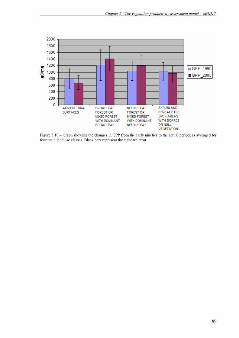
Chapter 5 - The vegetation productivity assessment model – MOD17
89
Figure 5.10 – Graph showing the changes in GPP from the early nineties to the actual period, as averaged for four main land use classes. Black bars represent the standard error.

Chapter 6 – The soil productivity assessment model - CENTURY
90
6. The soil productivity assessment model - CENTURY
6.1. Introduction
Several areas of the world are particularly vulnerable to environmental changes (Warren et al., 1996) or are degraded (UNEP, 1992), because of the reduction in the permanent plant cover (Le Houérou, 1995). This degradation includes reduced Soil Organic Carbon (SOC) levels, lower soil nutrient content, lower water holding capacity and increased risk of erosion (Batjes, 1999). Conversion of native land to cultivated land generally decreases SOC. The understanding of SOC dynamics and SOC distribution at a regional level is an essential step when quantifying regional and global C budgets (Paustian et al., 1997). The modelling of SOC content is a way of indirectly assessing C sequestration to complement direct measurements. Modelling may also help in the identification of areas with a large potential for increased SOC sequestration as well as making it possible to predict and understand future changes due to changing climate, altered land use and different land management practices. To be successful, these models need to incorporate both human and environmental factors when predicting regional SOC changes. The linking of dynamic simulation models to spatially explicit data permitted refined estimates of potential SOC sources and sinks, including their variation in space and time. Many severely degraded semi-arid environments have probably lost substantial amounts of SOC during the last century (Lal, 2001). Potentially, this loss could be counteracted through land management, accomplishing a positive contribution to local soil properties in addition to a simultaneous uptake of atmospheric CO2.
6.2. Description of the model CENTURY is a ‘lumped parameter’ ecosystem model simulating biogeochemical fluxes of C, N, P and S, primary production and water balance on a monthly time step (Parton et al., 1987; 1988; Metherell et al., 1993). The primary purpose of the model is to supply a tool for ecosystem analysis enabling the evaluation of changes in climate and the management of ecosystems. Originally it was developed to study Soil Organic Matter (SOM) dynamics in grassland soils (Parton et al., 1987), but it has been modified and expanded to simulate agricultural systems (Cole et al., 1989) and savannah systems. Driving variables are monthly precipitation and monthly average minimum and maximum temperatures. Soil texture, litter N, lignin content and tillage disturbance are also important soil characteristics. It is possible to include the effects of fires, fertilization, irrigation, grazing, various cultivation and harvest methods, etc. in the simulations. The model was widely used and validated (Burke et al., 1989; Parton et al., 1993; 1994; 1996; Bromberg et al., 1996; Smith et al., 1997; Mikhailova et al., 2000) for various ecosystems of Central and North America, Africa, Europe and Asia against field observations of soil organic matter dynamics (Parton et al., 1987; 1988). Values of parameters that control these routines are generally not altered in calibration of the model to a particular site. The model operate using general principles: i) the plant residue decomposition and the SOM content are based on soil texture, structure and composition; ii) the soil temperature, influencing the process of the microbiologic degradation of SOM, increase exponentially with the increasing of environmental temperature, whereas the soil moisture is a function of precipitation and potential evapotranspiration. In this case we used the CENTURY model to simulate dynamics of SOC in the soil estimating the crop, forest and grassland productivity. The version 4.0 of the model, whose scheme is represented in Figure 6.1, was used in our simulation. It was developed with the aim of including a large number of crop systems and management (crop rotations, tillage practices, fertilization, irrigation, grazing, and harvest

Chapter 6 – The soil productivity assessment model - CENTURY
91
methods), with the aim of analyzing the management and climate change effects over the productivity and the sustainability of crop ad forest systems.
Figure 6.1 – Scheme showing the structure of the CENTURY model.
In the Figure 6.2 we described an example of processes simulated inside the model for forest ecosystem.
Figure 6.2 - Compartment diagram for the Forest CENTURY model. The soil organic matter (SOM) component has several individual pools not shown in this figure (from Ryan et al., 1996).
6.2.1. Examples of validation of the model
Century model and the used parameters for the different classes of land use were validated through the analysis of results of more than 800 experiments and more than 60 experimental stations. Examined database contains studies on various type of land use. In general, long term experiments (1-5 years) were carried out for a validation of the model at global scale. In particular it has been developed a database by the CASMGS (Consortium for Agricultural Soils Mitigations of Greenhouse Gases - USA) containing results of experiments regarding soil carbon content changes according to land use and management practices. Results refer to validation experiments both in America and in Europe and constituted a suitable validation support for the

Chapter 6 – The soil productivity assessment model - CENTURY
92
present study. The field measurement data reported in literature were used to evaluate the result of CENTURY in our application on a land use basis. These validation data contain measures of SOC in the soil and show a good correlation with the results of CENTURY model in the same sites of measurement, as we can see in Figure 6.3, where there is a comparison between simulated and measured SOC for a grazed area.
Figure 6.3 - Comparison between measured and simulated SOC (right) quantities (from Zhang et al., 2007). Following graphs (Figure 6.4) show, for different land uses and management, a comparison between the measured and simulated soil organic carbon content:
Figure 6.4 – Comparison between C values measured and simulated by CENTURY (http://www.nrel.colostate.edu/projects/century/Century_Slides.ppt) In the following (Figure 6.5) it is reported the result of a CENTURY simulation regarding the first 20 cm of soil, compared with measured quantities, showing a good correlation. (r2 = 0.93).

Chapter 6 – The soil productivity assessment model - CENTURY
93
Figure 6.5 – Comparison between measured and simulated C quantities for the first 20 cm of soil (http://www.nrel.colostate.edu/projects/century/Century_Slides.ppt).
Finally they are reported (Figure 6.6) the correlations between measured and simulated quantities of soil organic carbon for different type of management.
Figure 6.6 – Comparison between the values of C in the soil as measured and simulated by the CENTURY for different types of management (http://www.nrel.colostate.edu/projects/century/Century_Slides.ppt).

Chapter 6 – The soil productivity assessment model - CENTURY
94
6.3. Production and format of input data
CENTURY model needs several input data and parameters, whose list is reported in Table 6.1. Input Unit of measure Mean of monthly precipitation amount cm/month Standard deviation of monthly precipitation amount cm/month Minimum air temperature at 2 meters °C Maximum air temperature at 2 meters °C Latitude of simulation site ° Longitude of simulation site ° Sand fraction in the soil unitless Silt fraction in the soil unitless Clay fraction in the soil unitless Soil density g/cm-3 Wilting point cm H2O per cm of soil Field capacity cm H2O per cm of soil pH Initial surface C with slow turnover (gC/m2) Initial soil C with slow turnover (gC/m2) Initial soil C with intermediate turnover (gC/m2) Initial soil C with fast turnover (gC/m2) Initial surface ratio C/N with slow turnover unitless Initial soil C/N ratio with slow turnover unitless Initial soil C/N ratio with intermediate turnover unitless Initial soil C/N ratio with fast turnover unitless Carbon content in the superficial litter (gC/m2) Carbon content in the soil litter (gC/m2) Initial C/N ratio of superficial litter with slow turnover unitless Initial C/N ratio of soil litter with slow turnover unitless Initial leaf C in forest ecosystems (gC/m2) Initial leaf C/N ratio in forest ecosystems unitless Initial wood C in forest ecosystems (gC/m2) Initial wood C/N ratio in forest ecosystems unitless Initial root C in forest ecosystems (gC/m2) Initial root C/N ratio in forest ecosystems unitless Initial carbon on death wood (gC/m2) Initial carbon on death root (gC/m2)
Table 6.1 – List of necessary input data to run CENTURY model All the data have been spatialized and included inside a unique database. These inputs are contained in a file with extension “.100”, whose preparation is described in Par. 6.3.8. This file is a text file containing all the input parameters and data for the model running (Figure 6.7). The file has two columns, the former with the value of parameters (according to the above cited units of measure), the latter with the correspondent variable name used in the model, formatted according to the requests of the model.
F

Chapter 6 – The soil productivity assessment model - CENTURY
95
Figure 6.7 – Example of a part of .100 file The .100 file production required a complex series of overlay, codifying and spatial analysis operations on order to generate the complete set of model parameters and inputs. For both the periods of simulation (early nineties and actual period) we created three “surfaces” of distribution to spatialize all the required inputs.
1. Forest Layer (FL) 2. Arboricolture Layer (AL) 3. Seeded cultivation Layer (SL)
That we will illustrate below. All these layers are in vector format with polygon geometry and they differ for the type of information reported: 1. FL contains the spatialized information about forest types from Corine Land Cover
database. It was created extracting from Corine Land Cover the land use classes relative to forest cover and re-classifying them in five macro-classes according to the following Table 6.2:
Corine Classes Century Classes 311 Broadleaf forest 312 Needleleaf forest 313 Mixed forest
322; 323; 324d Mediterranean “macchia” 321 Grassland/Pasture
Table 6.2 – Reclassification of the Corine Land Cover forest classes 2. AL contains the spatialized information about arboricolture from Corine Land Cover
database. It was created extracting from Corine Land Cover the four classes in Table 6.3:
CORINE Classes CENTURY classes 221 Vineyard 222 Orchard 223 Olive-Grove
2122 Rice Table 6.3 –CORINE LAND COVER arboriculture classes used to create AL
3. SL contains the spatialized information about crop types from seeded cultivation database. It was created by merging three different informatic layers (see Annex A): - Corine Land Cover - Map Sheet at scale 1:2000 (MS) - Crop data from AGEA (Italian Agriculture Agency, see Annex A)

Chapter 6 – The soil productivity assessment model - CENTURY
96
The alphanumeric tables relative to seeded cultivation supplied by AGEA were spatialized over the regional territory of Sardinia through a join between the MS and the relative cultivation code on the tables. For each polygon they are associated more than one cultivation. The MS was then overlaid with the CORINE LAND COVER classes reported in Table 6.4, in order to individuate, within each MS, the area effectively characterized by an agricultural use, excluding all other uses (Figure 6.8).
CORINE Classes
21 (except 2122; 2123; 2124) 24
Table 6.4 –Corine Land Cover seeded cultivation classes used to create SL
Figure 6.8 - (Left) MS before intersection with CORINE class 2; (Right) MS after intersection with CORINE class 2
Then we merged FL, AL and SL to form a unique informatic layer: the spatialization basis (SB), a polygon layer with associated a table with a “Type” field containing following “values”: “AGEA”: for the seeded cultivation polygons from SL “BROADLEAF”: for polygon relative to broadleaf forest from FL; “NEEDLELEAF”: for polygon relative to needleleaf forest from FL; “MIXED”: for polygon relative to mixed needleleaf and broadleaf forest from FL; “MACCHIA”: for polygon relative to Mediterranean Macchia from FL; “GRASSLAND”: for polygon relative to grassland/pasture from FL; “VINEYARD”: for polygon relative to vineyard from AL “OLIVE”: for polygon relative to olive-grove from AL “ORCHARD”: for polygon relative to orchard from AL “RICE”: for polygon relative to rice from AL This layer was used for further overlay operations useful to associate to each polygon several pedologic, climatic and vegetation parameters, as described in the next paragraphs.

Chapter 6 – The soil productivity assessment model - CENTURY
97
6.3.1. Textural data
The sand, silt, clay fractions have been included crossing the Pedologic Map and SB and further reclassifying resulted layer according to the Table 3.5.
6.3.2. Field capacity and wilting point These two input data were obtained applying a series of pedotransfer functions related to textural characteristics of the soil (Saxton et al., 1986):
%))*%*10285.4%*1088.4%*0715.0396.4exp( 2524 claysandsandclayA −− ⋅−⋅−−−=
%))*%*10484.3%*00222.014.3( 252 claysandclayB −⋅−−−= where clay% is the percent content of clay silt% is the percent content of silt sand% is the percent content of sand At this point, the raw wilting point (wp_raw) was calculated from:
B
Arawwp
1
15_ ⎟⎠⎞
⎜⎝⎛=
and the raw field capacity (fc_raw): B
Arawfc
1
33.0_ ⎟⎠⎞
⎜⎝⎛=
Then we applied several corrections in order to compute the final wilting point (wp) and the field capacity (fc) (http://www.nrel.colostate.edu/projects/century/soilCalculatorHelp.htm):
)_*15.0(_ rawwprawwpwp −+=
)_*07.0(_ rawfcrawfcfc +=
6.3.3. Density As this input is an attribute of the Pedologic Map, it was included in the database for the CENTURY model by the union of SB with the Pedologic Map.
6.3.4. Soil Organic Carbon (SOC)
To derive this input, we crossed the Pedologic Map (from which we have the soil organic matter content in %) and the SB layer and then we applied following relationship to the resulting map in order to derive the SOC: (SOM *density)/100 = SOM in g/cm3 (SOM g/cm3*20cm) = SOM in g/cm2 (SOM g/cm2 * 10000) = SOM in g/m2 As SOM/SOC=1.7, then SOC in g/m2= SOM in g/m2/ 1.7

Chapter 6 – The soil productivity assessment model - CENTURY
98
6.3.5. Climatic data
The climatic variables useful for running the model are: 1) Mean of the monthly precipitations (cm); 2) Standard deviation of the monthly precipitations (cm); 3) Mean of monthly maximum temperatures (°C); 4) Mean of monthly minimum temperatures (°C).
This values have been computed over two periods of thirty years, using the data from 1961 to 1990 for the simulation of the early nineties period, and the data from 1971 to 2000 for the recent period, including for the nineties the data spatialized by the Laboratorio di Simulazioni Numeriche del Clima e degli Ecosistemi Marini (University of Bologna, Italy). To associate to each polygon of SB a value of above cited climatic variables, we made a zonal statistic using the polygons itself as zone layer and calculating the means of those variables inside each unit of the polygon layer.
6.3.6. C and N of litter, roots, stems and leaves
To include data about C and N of the various vegetation/soil components, we used a series of codifying tables from literature (Table 6.5) applied only to the forest and arboriculture components (except the rice class).
Needleleaf Broadleaf Forest and
arboricolture
MixedForest
MediterraneanMacchia Parameter Unit of
measure
4.4 28.4 16.4 59 C soil 10^3 kg/ha 0.25 2.825 1.538 5.9 N soil 10^3 kg/ha
8 1 4.5 2 C Foliage 10^3 kg/ha 63 84 73.5 21.4 C stem 10^3 kg/ha 25 24 24.5 11 C coarse root and/or stump 10^3 kg/ha 1.4 2.4 1.9 0.58 C fine root 10^3 kg/ha
Table 6.5 –Values of some parameters requested by the model and relative to C and N contents in soil/vegetation components.
6.3.7. Final database
The last operation was adding a numeric ID for identifying each polygon of the SB. As the model ran one time for each polygon (having homogeneous characteristics) but offline from GIS environment, by means of field “ID” it has been possible to fast associate (to spatialize) the results in to the initial map. At the end of all the overlay, union, intersection and re-classifying operations above described, SB consisted in a vector layer with associated a table containing all the requested parameters. (Figure 6.9).

Chapter 6 – The soil productivity assessment model - CENTURY
99
Figura 6: Base di spazializzazione Figure 6.9 –Final Map SB of polygon units for which the model has run, the table of attribute of vector data contains, for each polygon, all the inputs required by the model. The land cover of each polygon determines the management applied to that polygon, i.e. the management is identical for each land cover type for the entire area. This was a necessary simplification as detailed management and crop information is lacking. In general, land management was based on interviews, field observations and literature (phenologic calendars and good agricultural practices handbook).
6.3.8. “.100” file creation As already said, the input required by CENTURY is a file with extension “.100” (Figure 6.7) for each location of simulation (in our case: a polygon). Then each record of the attribute table of SB was converted in file ”.100” To do this a GUI tool was written in Visual Basic (named file100.exe) in order to automate and make faster the process of creating input files and directories (Figure 6.10) as requested by the model.

Chapter 6 – The soil productivity assessment model - CENTURY
100
Figure 6.10 - Tool written in Visual Basic to create automatically input files and directories requested by CENTURY.
6.3.9. Output structure
The final output consisted in two tables that were spatialized into the vector SB layer and then this layer was rasterized into two grids representing the simulated spatialized value of soil organic carbon (gC/(m2*year)) for each period of simulation, that is assumed as the soil productivity.
6.4. Simulation and result discussion For the CENTURY model two simulations were carried out: the former with data relative to the early nineties (first period of simulation), the latter with data relative to the actual period (second period of simulation). In each simulation the first 1000 years of simulation without management served to allow to system to reach the equilibrium, using stochastic meteorological data generated from the existing ones. All spatially distributed data used were in vector format, for each polygon with a unique combination of spatially distributed variables (soil texture, precipitation, land cover, crop-type and management etc.), the CENTURY model was executed once. This reduced the number of model executions, avoiding redundant calculations and hence reducing the calculation time significantly. After simulations, considering the typical values of soil productivity according to the land use and management, an analysis of obtained results for the Sardinia regions was carried out. Field measurements from literatures were used to evaluate the results of the CENTURY model. Figure 6.11 shows the differences between the two simulations for four main land use classes, suggesting that forested areas suffer from a decrease of soil fertility, whereas the agricultural areas and the other natural areas, with less vegetation, have had a little increase of SOC.

Chapter 6 – The soil productivity assessment model - CENTURY
101
Figure 6.11 – Comparison, for the two reference periods, of SOC (gC/m2) per year vs. four main categories land use classes. Black bars represent the standard error. Looking at the results on a land use basis with a larger detail (Figure 6.12), the 331 Corine Land Cover class (sand, dunes, beaches) demonstrated a large diminution of soil organic carbon, but this class has no vegetation and so it is already without organic carbon and then it is not interesting for our purposes. Other classes are present only in the most recent database and then we cannot consider them for a comparison with the past.
0
1000
2000
3000
4000
5000
6000
7000
8000
9000
10000
211
212
213
221
222
223
231
241
242
243
244
311
312
313
321
322
323
324
333
334
soc_1990soc_2005
Figure 6.12 – Comparison, for the two reference periods, of soil organic carbon (gC/m2) per year vs. the land use classes (CORINE LAND COVER CLASSIFICATION). Black bars represent the standard error. We can conclude that the SOC content had not great variation between the two periods according to the model results. The reason could be that the model is highly sensitive to the management practices similar in the two periods of simulation, then we can suppose CENTURY could be a more useful instrument mainly for long term simulations, where these two most influencing inputs can have a more evident variability. In the following we report the maps (Figure 6.13) of CENTURY results relative to SOC (gC/m2) in the soil where it is clear the spatial distribution of results.

Chapter 6 – The soil productivity assessment model - CENTURY
102
Figure 6.13 – Results of the CENTURY model showing the spatial distribution of SOC values (gC/m2*year). But the CENTURY model has many other outputs, one of which concerning the vegetation productivity NPP (Net Primary Production in gC/m2*year): we reported the graph (Figure 6.14) relative to the mean quantities for each land use, according to the classification already used for the MOD17 model (see Table 5.4), in order to compare the outputs of the two models (NPP for CENTURY and GPP for MOD17).
Figure 6.14 – Comparison, for the two reference periods, of vegetation productivity (NPP, in gC/m2) per year vs. the land use classes (the same reclassification used to evaluate MOD17 results, see Table 5.4). Black bars represent the standard error.
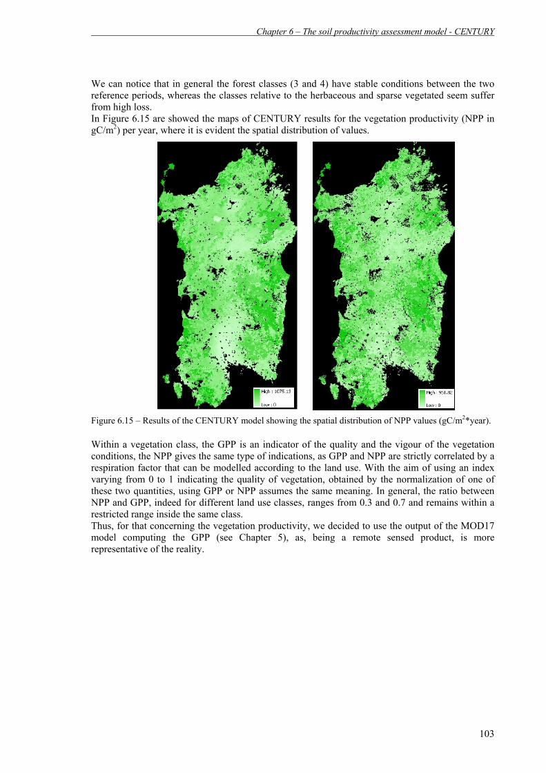
Chapter 6 – The soil productivity assessment model - CENTURY
103
We can notice that in general the forest classes (3 and 4) have stable conditions between the two reference periods, whereas the classes relative to the herbaceous and sparse vegetated seem suffer from high loss. In Figure 6.15 are showed the maps of CENTURY results for the vegetation productivity (NPP in gC/m2) per year, where it is evident the spatial distribution of values.
Figure 6.15 – Results of the CENTURY model showing the spatial distribution of NPP values (gC/m2*year). Within a vegetation class, the GPP is an indicator of the quality and the vigour of the vegetation conditions, the NPP gives the same type of indications, as GPP and NPP are strictly correlated by a respiration factor that can be modelled according to the land use. With the aim of using an index varying from 0 to 1 indicating the quality of vegetation, obtained by the normalization of one of these two quantities, using GPP or NPP assumes the same meaning. In general, the ratio between NPP and GPP, indeed for different land use classes, ranges from 0.3 and 0.7 and remains within a restricted range inside the same class. Thus, for that concerning the vegetation productivity, we decided to use the output of the MOD17 model computing the GPP (see Chapter 5), as, being a remote sensed product, is more representative of the reality.
Chapter 7 – The wind erosion assessment model - WEAM
104
7. The wind erosion assessment model - WEAM
7.1. Introduction
According to UNCCD and then to a European approach (DESERTLINKS project), wind erosion is an indicator of desertification and interacts with other (biophysical and socio-economic) indicators of land degradation. Various effects derive from soil erosion by wind: - the on-site effects are damages to crops, loss of fertile topsoil and loss of soil structure resulting in yield reduction and the need for additional inputs, and the long term soil degradation; - the off-site effects are mainly the result of dust penetration into residential areas (visibility reduction and health hazard) and into machinery. The wind erosion, whose main consequence is the loss of superficial soil, is very frequent in southern Europe. The removing of soil material is selective, much more than for the water erosion, as only the most fine particles (clay and organic matter), with their nutrient loading, are taken away leaving only a poor soil with a coarse texture. Besides the direct effect of removing soil, other indirect effects of the phenomenon regard the atmospheric pollution because of the presence of dust particle, the cover of the most fertile layers of soil and, in most extreme cases, the complete cover of areas and the formation of dunes. They exist three types of dynamics occurring over a soil interested by wind erosion: creep is the phenomenon whereby soil particles larger than ~1000 µm and soil aggregates that are too large to be picked up by wind move along the ground because of wind forces and impact with other soil grains. In the process of saltation, some grains are lifted by the air but fall back to the surface after a short distance. Saltation can be thought as the horizontal flux of soil across the surface. These are the most damaging particles for crops. Saltating particles also lead to suspension of smaller particles including PM10 (ten micron diameter Particulate Matter). Suspension occurs when grains smaller than ~20-30 µm become entrained in turbulent air motion and are transported to long distances. The vertical flux of dust corresponds to the mass of particles suspended. As for other degradation processes, there are natural and predisposing conditions to erosive agent, but also human activities play a key role in favouring wind erosion. For example, among the acknowledged causes the overgrazing seems to be the most influencing factor, not neglecting the fact that the most sensitive areas to wind erosion are the ones less suitable for other uses. Figure 7.1 show the extent of areas vulnerable to wind erosion according to U.S. Department of Agriculture, Natural Resource Conservation Service (USDA-NRCS)
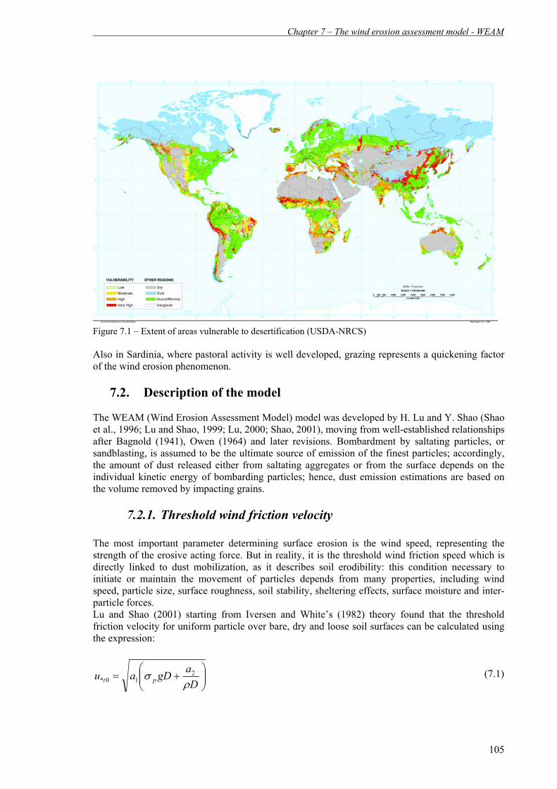
Chapter 7 – The wind erosion assessment model - WEAM
105
Figure 7.1 – Extent of areas vulnerable to desertification (USDA-NRCS) Also in Sardinia, where pastoral activity is well developed, grazing represents a quickening factor of the wind erosion phenomenon.
7.2. Description of the model
The WEAM (Wind Erosion Assessment Model) model was developed by H. Lu and Y. Shao (Shao et al., 1996; Lu and Shao, 1999; Lu, 2000; Shao, 2001), moving from well-established relationships after Bagnold (1941), Owen (1964) and later revisions. Bombardment by saltating particles, or sandblasting, is assumed to be the ultimate source of emission of the finest particles; accordingly, the amount of dust released either from saltating aggregates or from the surface depends on the individual kinetic energy of bombarding particles; hence, dust emission estimations are based on the volume removed by impacting grains.
7.2.1. Threshold wind friction velocity
The most important parameter determining surface erosion is the wind speed, representing the strength of the erosive acting force. But in reality, it is the threshold wind friction speed which is directly linked to dust mobilization, as it describes soil erodibility: this condition necessary to initiate or maintain the movement of particles depends from many properties, including wind speed, particle size, surface roughness, soil stability, sheltering effects, surface moisture and inter-particle forces. Lu and Shao (2001) starting from Iversen and White’s (1982) theory found that the threshold friction velocity for uniform particle over bare, dry and loose soil surfaces can be calculated using the expression:
(7.1)
⎟⎟⎠
⎞⎜⎜⎝
⎛+=
DagDau pt ρ
σ 210*
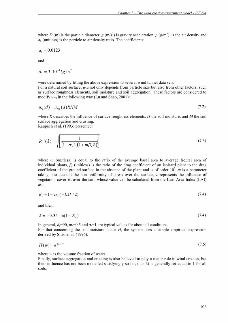
Chapter 7 – The wind erosion assessment model - WEAM
106
where D (m) is the particle diameter, g (m/s2) is gravity acceleration, ρ (g/m3) is the air density and σp (unitless) is the particle to air density ratio. The coefficients:
0123.01 =a and
242 /103 skga −⋅=
were determined by fitting the above expression to several wind tunnel data sets. For a natural soil surface, u*t0 not only depends from particle size but also from other factors, such as surface roughness elements, soil moisture and soil aggregation. These factors are considered to modify u*t0 in the following way (Lu and Shao, 2001):
(7.2)
where R describes the influence of surface roughness elements, H the soil moisture, and M the soil surface aggregation and crusting. Raupach et al. (1993) presented:
(7.3)
where σr (unitless) is equal to the ratio of the average basal area to average frontal area of individual plants, βr (unitless) is the ratio of the drag coefficient of an isolated plant to the drag coefficient of the ground surface in the absence of the plant and is of order 102, m is a parameter taking into account the non uniformity of stress over the surface, λ represents the influence of vegetation cover Ev over the soil, whose value can be calculated from the Leaf Area Index (LAI) as:
(7.4) and then:
(7.4)
In general, βr=90, mr=0.5 and σr=1 are typical values for about all conditions. For that concerning the soil moisture factor H, the system uses a simple empirical expression derived by Shao et al. (1996):
(7.5)
where w is the volume fraction of water. Finally, surface aggregation and crusting is also believed to play a major role in wind erosion, but their influence has not been modelled satisfyingly so far, thus M is generally set equal to 1 for all soils.
RHMdudu tt )()( 0** =
( )( )⎥⎦⎤
⎢⎣
⎡+−
=−
λβλσλ
rr mR
111)(1
)2/exp(1 LAIEv −−=
)1ln(35.0 vE−⋅−=λ
wewH 7.22)( =

Chapter 7 – The wind erosion assessment model - WEAM
107
7.2.2. Horizontal and vertical fluxes
Following Lu and Shao (1999), WEAM predicts size-resolved dust fluxes F(d) (gm-2s-1) as:
(7.6)
where d is the particle diameter (m), Q(d) (kg m-1s-1) is the size-resolved horizontal flux of saltating particles, Cα is a coefficient of order 1, g (m/s2) is the gravity, f is the total volumetric fraction of dust in the sediment, ρp is the bulk soil density (kg m-3) and p (N m-2) is the soil penetration resistance. The horizontal flux Q(d) can be before modelled as (Owen, 1964):
(7.7)
where the coefficient c is of order 1, ρ (kg m-3) is the air density, u* (m s-1) is the actual friction velocity and u*t (m s-1) is the threshold friction velocity. According to all that just explained, we can understand the direct input data of the model are:
• Particles Size Distribution • In situ density (g/cm3) • Particle density (g/cm3) • Vegetation roughness (basal area/frontal area) • Volumetric water content of soil (%) • Friction wind velocity (m/s) • Non erodible elements fraction coverage • Penetration resistance (N/m2)
According to the availability of these data or the existence of other data useful to derive them, we made some modification to the model algorithm as illustrated in par. 7.3.
7.2.3. Examples of validation of the model
The flux estimated by the model (t/ha*year) is directly proportional to concentration, in the air, of emitted particles (µg/cm3). As the concentration measurements are more common than the flux measurements, validation experiment of WEAM model carried out by developer team regarded the comparison between observed and simulated concentration, as shown in the following graphs in Figures 7.2 and 7.3.
)(12.0
)( dQp
gfCdF pρα=
⎩⎨⎧
<≥−
=)(0)(])/)((1)[/(
)(**
**2
**3*
duuduuuduguc
dQt
ttρ

Chapter 7 – The wind erosion assessment model - WEAM
108
Figure 7.2 – Comparison between observed and WEAM-modelled TSP (Total Suspended Particles) concentration (Shao et al., 2003)
Figure 7.3 – Comparison between observed and WEAM-modelled particle concentration, with a diameter less than 11 micron (left) and 2 micron (right). (Shao et al., 2003) In following Table 7.1 we reported other results of validation experiments, where for events with several day duration, we can notice the good agreement between simulated and observed data.

Chapter 7 – The wind erosion assessment model - WEAM
109
Table 7.1 – Comparison between TSP (Total suspended particle) concentration (µg m-3) as observed (Cobs) and modelled (Cmod) by WEAM for several events (modified from Shao et al., 2003). Plotting these results in a graph (Figure 7.4) shows an R2 of about 0.73.
R2 = 0.7353
1
10
100
1000
10000
1 10 100 1000 10000
Figure 7.4 – Correlation between observed and modelled concentration values relative to events listed in Table 7.1. The unit of measure of the quantities on the logarithmic axes is (µg m-3)

Chapter 7 – The wind erosion assessment model - WEAM
110
7.3. Parameterization and modifications to the model Starting from the supplied source code of the model, whose programming language is FORTRAN 90, the same language was used to introduce several modifications to the code until the creation of an executable file WEAM_sar.exe, where “WEAM” is the model name and “sar” stands for Sardinia.
7.3.1. Particle Size Distribution The original edition of Shao & Lu code considers four types of soil (sand, sandy loam, loam, clay) and for each there are two types of particle size distribution already parameterized within the source code. One is the fully dispersed particle size distribution, regarding the soil composition when it is fully disaggregated, that provides a resultant ‘percentage clay’ parameter which is an efficient index of soil capability to form micro-aggregates. Another one is the minimally dispersed particle size distribution which reflects soil in-situ size distribution. For the WEAM theory, the Particle Size Distribution (PSD) of removed volume can be modelled by weighting the distribution aforementioned. In our study, we distinguished five textural classes (coarse, medium, medium-fine, fine, very fine) according to the textural triangle of Figure 3.3, that, starting by percent composition of sand, silt and clay, allowed also to reclassifying the field of texture description of the Pedologic Map according to Table 3.5 (fully dispersed distribution). These textural compositions were used to reconstruct synthetic distributions whose parameters (mean, standard deviation) are read by the model and utilized in the flux integration above described. Udden (1914) and Wentworth (1922) were among the first ones to conclude that particle-size distributions (PSDs) are log-normal and in general a number of modes from 1 to 4 are enough to describe distribution. This means that both types of distribution, for each population (mode) composing them, can be represented by the formula:
(7.8) where p(d) represent the function distribution for a given diameter, d is the diameter, wi the fraction of the population in respect to the total, σi is the standard deviation of that population, Di is the mean diameter of population. First, starting from textural distribution of a soil without aggregates (fully dispersed) that is the one in the Pedologic Map of Sardinia as is the standard distribution used in sedimentology, it was necessary to model an other type of distribution, that is the one related to the presence of soil aggregates and then the most representative of in-situ conditions (minimally dispersed). This was done using the relationships already illustrated in Figure 3.4. Results of this modelling procedure are shown in Tables 7.2. Table 7.2 – For each type of soil in the Pedologic Map of Sardinia, the textural percent content of minimally dispersed distribution.
Textural class clay (%) silt (%) sand (%)
coarse 2 13.6 84.4
medium 4.60 40.40 55.00
medium fine 4.40 76.00 19.60
fine 12.00 0.00 88.00
very fine 76.80 16.80 6.40
( )⎟⎟⎠
⎞⎜⎜⎝
⎛ −−
=∑= i
iDd
i
in
iew
ddp σ
πσ2
lnln
1
2
21)(

Chapter 7 – The wind erosion assessment model - WEAM
111
A size-frequency curve-fitting program called MIX 3.1, developed by Macdonald and Green (1988) for ecological population studies, was here used to perform these sediment population analyses. For each MIX analysis, we must first estimate the mean, proportion and standard deviation of each component population within a PSD and enter them as input parameters. A Chi-Squared (χ 2) statistic is used by the software to test the goodness-of-fit. Graphical output (Figure 7.5) is in the form of a particle-size relative frequency histogram with best-fit normal frequency curves for each population within the total PSD.
Figure 7.5 – Example of graphs of mixed textural distribution of soil given by several (four in this case) log-normal distributions, for the medium textural class reported in Pedologic Map. Fully dispersed soil (left) and minimally dispersed (right). From these distributions, the software extracted the statistical parameters, whose an example is shown in Table 7.3, for the medium textural class.
Table 7.3 – Example of parameters of modes of granulometric distribution implemented in the model and referred to the medium class of the Pedologic Map of Sardinia. Also according to the soil density parameter ρp (kg/m3), we introduced its computation starting from textural data in the Pedologic Map of Sardinia, following the theory of Saxton (1986):
(%)))log*1276.0((%))*4251.7(668.0(*65.2*920 10 clsap −−+=ρ (7.9) were sa(%) is the sand percent content and cl(%) is the clay percent content.

Chapter 7 – The wind erosion assessment model - WEAM
112
7.3.2. Wind friction velocity
Further modifications to the model regarded the accounting for the temporal variability for some inputs, in particular, given the high sensitivity of the model to soil moisture and to vegetation presence, we considered daily and seasonal variability, respectively, of these two inputs, working inside the code to derive from these data the model parameters.
7.3.2.1. Soil moisture factor
It is worth saying that moisture content is a key parameter for assessing water role in particle interspaces (Fècan et al., 1999) and the model has been proven to be highly sensible to its value. Several studies (e.g. Ravi, 2001) suggest that wind erosion is mainly affected by the highly variable moisture content of the first few millimetres of soil, whose primary source is atmospheric humidity. Wind tunnel tests (Gregory and Darwish, 1990) showed that atmospheric humidity plays an important role in determining moisture content at the soil surface, where wind indeed exerts its stress. This dependence from air humidity is significant especially in arid environments and seasons. Accordingly, we attempted to model soil moisture w for more superficial soil (few millimetres) on the basis of the air relative humidity (RH). From the latter parameter, the soil matrix potential (ψ) is derived from the following theoretical relation:
(7.10)
where R is the gas constant (8.31 J/mol K), M is water’s molecular weight (g) and T the absolute air temperature (K). RH was calculated starting from the meteorological daily data about mean temperature and dew point temperature (both in °K)
(7.11)
where lv = latent heat of vaporization of water (2.5E6 J/Kg), Rv = gas constant for water vapor (461.5 JK / Kg), Td = dew point temperature (°K) and T = temperature (°K). Then, we inverted the empirical relation in (Gardner, 1970) to derive volumetric soil moisture from matric potential Ψ :
(7.12)
where a and b are parameters depending on the soil type (Saxton et al., 1986). Although many studies about the effect of sediment water content on aeolian transport related such dynamics to the water content on a volumetric base (w, m3/m3), this parameter does not contain information on how tightly the water is held by the soil. However, Chepil (1956) and Chen et al. (1996) consider inter-particle forces developed by the adsorbed water film being much lower than inter-particle capillary forces. Capillary forces, which are referred to as the water potential (w’), induce a reinforcement of cohesion and are more closely associated with soil texture and structure; indeed the water potential around the grains is negligible for sands and increase with clay percent content, following a second order polynomial equation (Fècan et al., 1999):
RHM
TR ln⎟⎠⎞
⎜⎝⎛ ⋅
=ψ
10011exp
11exp
0
0 ⋅
⎟⎟⎠
⎞⎜⎜⎝
⎛⎟⎟⎠
⎞⎜⎜⎝
⎛−⋅
⎟⎟⎠
⎞⎜⎜⎝
⎛⎟⎟⎠
⎞⎜⎜⎝
⎛−⋅
=
TTRl
TTRl
RH
v
v
dv
v
baw −=ψ

Chapter 7 – The wind erosion assessment model - WEAM
113
(7.13) Thus, in this study the soil moisture enlargement factor H was parameterized as:
(7.14) (7.15)
7.3.2.2. Roughness factor
Natural vegetation has a twofold role in protecting soil from wind erosion: it absorbs part of the wind momentum by increasing surface roughness (Stockton and Gillette, 1990) and protects the soil surface from erosion, both by direct sheltering and by providing a “wake area” with high turbulence and zero mean velocity. Soil erosion also depends on the presence of clods, rocks, crop residues etc. (Raupach et al., 1993), that can be treated together as non-erodible elements. Experimental studies showed that wind erosion thresholds observed on rough surfaces are significantly higher than those observed on smooth surfaces (Gillette and Stockton, 1989). Thus, also amount, stability and geometry of aggregates on the surfaces are a major factor affecting susceptibility of soil to wind erosion. The impact of roughness elements on threshold wind friction velocity (R) was modelled, following Raupach et al. (1993), as:
(7.16)
where the first term under the square root accounts for coverage, while the second accounts for drag; λ is the roughness density, σ is the basal-to-frontal area ratio (commonly assumed to be 1); m is a parameter indicating uniformity (if 1) or non-uniformity (if <1) of the surface stress: m=0.5 was assumed here; β is the ratio of the drag coefficients of roughness element over that of the bare soil, β=CR/CS. Numerous studies (e.g. Crawley and Nickling, 2003; Raupach et al., 1993, Okin and Gillette, 2004) assessed β at about 90-100 for vegetated surfaces and 1 for bare soils; these values were also used here as showed later.
7.4. WEAM simulation Tool The WEAM model, among all the models used in the present work, was the one with the longest simulation time and with large impact over internal resources of the processor. Indeed it works on a daily basis according to the time steps of climatic input data, and it need to make two mathematical integrations, the former over the interval of saltating particles and the latter over the interval of suspended particle. We developed then a tool named WEAM (Figure 7.6) by means of VB programming language, that make a “partitioned” simulation on a 5-days basis: in particular it creates regularly the input file for the model every 5 days of simulation, and finally sum the 73 (number of 5-days intervals in a year) outputs in a final map of quantity of vertical flux (gm-2s-1). This tool use GIS format as input and output, but it runs offline by GIS.
%)(17.0%)(0014.0(%)' 2 clclw +=
( )[ ] ''21.11'1
5.068.0 wwforwwHwwforH
>−+=
<=
( )( )βλλσ mR +−= 11

Chapter 7 – The wind erosion assessment model - WEAM
114
Figure 7.6 – Image showing the window to start WEAM simulation, dividing it into 73 runs, one every 5 days.
7.5. Production and format of input data
The model was written in order to deal with one of the most common GIS formats (an ESRI owner format), in particular the ASCII grid format already explained. It was necessary the perfect spatial correspondence of cell borders and of no data distribution, as explained in the Chapter 3 (par. 3.4). We list in the following the input data required to implement the model, their units of measure, the necessary time step and the format of data. In particular four datasets have been at the basis of derivation of input data for the WEAM model: the Corine Land Cover Database, the Pedologic Map of Sardinia, produced specifically for the project, the remote sensed LAI, and the climate dataset. The detailed description of these datasets is contained into the Annex A, but here we want to remember that for some inputs (Corine Land Cover, LAI and climatic datasets) the processing operations described in the following were done for two sets of data, the first relative to early nineties period and the second relative to the actual period.
7.5.1. Erodible areas We stated to consider for running of the model only the really erodible parts of the territory. To do this we reclassified the field of texture description of the Pedologic Map according to Table 3.3 (see Par. 3.4.1).
7.5.2. Soil roughness
It represents the roughness height (cm) of vegetation, given to each type of land use by means of a Look Up Table (Pineda et al., 2004) and distinguished between the summer-spring and the winter-autumn seasons. This parameters served to calculate wind friction velocity starting from the wind velocity. To codify this input we use the Corine Land Cover databases for the two periods of interest, giving to each class a value using following Table 7.4.

Chapter 7 – The wind erosion assessment model - WEAM
115
Table 7.4 – Value used to codifying the roughness height of vegetation according to the Corine Land Cover classes
These inputs data from vector format has been converted in grid format.
7.5.3. Textural composition
Clay content (particle smaller than 0.064 mm), silt content (particle between 0.064 mm and 2 mm) and sand content (particle larger than 2 mm), all in percent, are necessary inputs for soil matric potential definition and for size distribution modelling. The field of texture description of the Pedologic Map was reclassified according to Table 7.5:
Class Clay(%) Silt(%) Sand(%) Coarse 7.9 13.6 78.6 Medium 17.6 40.4 42.0 Medium fine 17.0 76.0 7.0 Fine 46.0 27.0 27.0 Very fine 73.3 13.3 13.3 Other 0 0 0
Table 7.5 - Codifying of the sand, silt, clay percent content of soil for the different textural classes contained into the Pedologic Map of Sardinia. With “other” we indicated the wet-urban areas of Pedologic Map. These inputs data from vector format of Pedologic Map have been converted in grid format.
7.5.4. Vegetation/soil drag coefficient
This parameter, previously called β, served to evaluate the R factor about the increase of threshold wind friction velocity. It is a parameter assessed by literature as equal to 90 in vegetated areas and equal to 1 in areas without vegetation (Okin and Gillette, 2004). The codifying was made considering the Corine Land Cover for the two periods of interest and using following classification in Tables 7.6 and 7.7:
CORINE 1990 classes Value CORINE 2003 classes Value 1;4;5;332 0 1; 4; 5;2123;2124;3315;332 0 331 1 3311;3312;3314 1 Remaining 90
Remaining 90 Tables 7.6 (left) and 7.7 (right) – Codifying of the Corine Land Cover classes to assign a value of β parameter. After reclassifying, we rasterized these vector layers obtaining two ASCII grids.
CORINE LAND COVER class Winter roughness Summer roughness 1 50.00 50.00 211, 212, 213, 231 5.00 15.00 221,222, 223, 241, 242, 243, 244 20.00 20.00 311, 312, 313 50.00 50.00 321 0.10 0.12 322, 323, 324 10.00 11.00 331, 332, 333, 334 10.00 10.00 4 20.00 20.00 5 0.01 0.01

Chapter 7 – The wind erosion assessment model - WEAM
116
7.5.5. Daily climatic data Climatic input data were: • Dewpoint Temperature (°K); • Mean Air Temperature (°K); • Wind speed (m/s). The wind velocity gives us an idea of the force of acting agent and it is directly used by the model to calculate the friction velocity useful to verify the overcoming of the threshold wind speed for the erosion and then the fluxes. The two temperature variables served to calculate, jointly with textural data, the soil moisture and the H factor increasing the value of the threshold wind friction velocity. The daily data were obtained by daily maps at 1 km of resolution, supplied by the Laboratorio di Simulazioni Numeriche del Clima e degli Ecosistemi Marini group (University of Bologna, Italy) and produced by spatializing the station data (for a maximum of 18 regional stations comprising the UCEA station and the NOAA stations, see Annex A) taking into account also relationships among climatic variables and topography. In particular, in order to work with a mean climatic year and not with a single year that could be not representative, we averaged the monthly data of five years of early nineties (1991-1992-1993-1994-1995), and of five years representing actual period (2001-2002-2003-2004-2005). Daily data were then ready to the input of model. We produced 365 (days) x 3 (parameters) x 2 (reference years) grids relative to climatic data. We created several automatic procedures by Python programming language (Figure 7.7), for the correct formatting:
Figure 7.7 – Part of the Python code written to format and homogenise climatic input data of WEAM
Resulting grids are ASCII grids, in particular 365 grids for each variable.
7.5.6. Leaf Area Index (LAI) The LAI data useful for reconstructing the temporal (8-days) variation of this variable were obtained for the periods of interest by MODIS sensor (MOD15A2 product for the actual period represented by images of the year 2003, Annex A). In order to derive LAI data for the early nineties period, comparable with the LAI relative to the actual period, we first calculated the relationships between the AVHRR NDVI (seeChapter 3 and Annex A) at 1 km of resolution and the MODIS LAI at 1 km of resolution, considering only the images regarding the same date interval, both for the year 2003, and working on a land use basis (third level of the Corine Land Cover database). After extracting the regression lines (with LAI-MODIS as dependent variable and NDVI-AVHRR as independent variable) for all the matching dates, these relationships were re-applied to the available NDVI-AVHRR images for the 1995 (reference year for the past periods of simulation) obtaining a “synthetic” LAI-MODIS for the year of reference.

Chapter 7 – The wind erosion assessment model - WEAM
117
Developed methodology to prepare images for input to the model consists in four different treatment phases for the images:
• Projection – Mosaicing – Cut of images (Annex A) • Gap Filling (Annex B) • Downscaling from 1000 m to 50m of resolution for the actual data (Annex C) • Downscaling from 1000 m to 50m of resolution for the past data (Annex D)
Both temporal datasets (LAI-MODIS for the years 1995 (derived) and 2003 (real)) contained images with numerous invalid values because of both cloud problems and sensor errors, so we carried out the gap filling of images to recover data using a methodology that for a given invalid pixel of an image make iteratively a mean of the pixel values between the previous and the next image (see Annex B for the explanation of the method). Then we made a downscaling first to 250 meter of resolution considering the MODIS-NDVI product at 250 m of resolution for the 2003 and then the land use map for the year 2003 to further downscaling to 50 m (Annex C). For the 1995 dataset we used the land use map for the year 1990 for downscaling it from 1000 m to 250 m of resolution, then this map has been re-sampled at 50 meters of resolution (see Annex D). Then from this set of LAI images we calculated seasonal averages at 50 meters of resolution, and these data were corrected for the missed data by using statistical analyses. Indeed the areas characterized by no_data because of lack of values in the original images, have been treated carrying out a zonal statistics between LAI datum and Corine Land Cover: for each land use class (considered at the third level of the dataset), we calculated the mean value of LAI, then this value was assigned to no_data areas present in the image according to their land use Figure 7.8).
Figure 7.8 - Zonal statistics: they have been computed the mean values of LAI on a land use basis (third level of Corine Land Cover) for the 2003 seasonally-averaged grids, then these values have been associated to the same land use classes where existed no-data.

Chapter 7 – The wind erosion assessment model - WEAM
118
Finally we masked the areas corresponding to the code 6 of the soil texture layer, where the model did not run.
7.5.7. Other input data
Further, besides spatialized data, we needed an input file for our model, input_weam.txt, containing 10 rows with the following information: 1st row: input data available and representative of soil moisture: 1=dew point temperature
(°K); 2=soil moisture (mm); 2nd row: method to calculate H factor: 1=Shao; 2= Fècan; 3rd row: day of begin of simulation; 4th row: number of days of simulation, set to 5; 5th row: year of simulation 6th-10th rows: julian day of simulation (e.g. 001, 002, 003)
7.6. Simulation and result discussion
Two simulations were made using the WEAM model, the former with a set of data relative to early nineties period (the chosen range of years is 1991-1995), the latter with a set of data relative to most recent situation (reference years 2001-2005). The output is a ArcINFO grid with associated, for each cell, the value of soil loss (t/ha*year) due to wind erosion. We show in the following (Figure 7.9) the maps resulted by two simulations. It is clear that, according to the wind regime and for the same land use, the areas interested by a not negligible wind erosion are in both periods mainly the ones of coastal sectors.
Figure 7.9 – The images show the WEAM results for the two periods of reference, the early nineties (left) and the actual period (right), the values are in t/(ha*year)

Chapter 7 – The wind erosion assessment model - WEAM
119
As explained, all that we made before running was a detailed daily reconstruction of climatic data (wind speed and temperature–based variable) to take into account the daily variability of several input data as atmospheric conditions and soil moisture. Also as regards the vegetation cover we tried to account for the seasonal variability as much as possible, mainly because the model is highly sensitive to this input. Leaving the strength of the erosive agent out of consideration, in the effort to highlight a land use more vulnerable than another to wind erosion, we cannot neglect a statistical descriptive analysis of erosion values inside each land use type, with the aim of extracting mean and range of values. Fort this reason we report in the Table 7.8 the distribution of mean and standard deviation of erosion values inside each land use class (third level Corine Land Cover) for the actual period. We can notice the phenomenon is limited to few classes, in particular to the agricultural ones. Indeed by analyzing data present in literature it is evident the importance of the phenomenon mainly for agricultural sites that suffer from frequent removing of soil, management changes and alternation of periods with more or less vegetation cover.
LAND USE CODE MEAN STD 211 0.02717 0.40798 212 0.05639 0.63981 221 0.60299 3.56874 222 2.88589 8.73840 223 0.16413 1.78427 231 0.00000 0.00000 241 0.07201 1.10625 242 0.81045 4.38202 243 1.07355 4.76903 244 0.14146 1.76461 331 13.94150 24.70080 333 0.06839 0.39080
Table 7.8 – Statistics of soil loss values (t/ha*year) for the land use classes for which the WEAM model ran
Unfortunately in literature there are scarce information about the assessment of wind erosion allowing to derive a “look up table” between land use and typical erosion values or at least a range of standard values for a given wind event. In particular the calibration experiments for the wind erosion models are over limited temporal scales (single events) and at a smaller spatial scale (grid with resolution of some km) because often these models are coupled with atmospheric circulation models. The extrapolation of annual values of erosion by event-based data is dangerous, if we cannot reconstruct as best as possible the temporal series of wind speed (erosivity) and the correspondent conditions on the ground (erodibility). These results have been compared with different databases present in literature and deriving from experimental results (they don’t exist experimentations made in Sardinia) allowing to confirm the erosion model validity as estimator of emitted particle quantity (see par. 7.2.3).

Chapter 8 – The saltwater intrusion assessment model - SHARP
120
8. The seawater intrusion assessment model - SHARP
8.1. Introduction The entity of soil salinization along the coasts, a typical problem of the Mediterranean areas, is somewhat difficult to estimate, both for the complexity of the process and for the temporal and spatial variability of the phenomenon itself. We can anyway distinguish between two types of salinization: the former related to natural causes, as the closeness of marsh and ponds, the latter linked to anthropogenic actions and due to an inappropriate use of water resources mainly for irrigation purposes. This second reason, triggered by an uncontrolled use of groundwater, can have in its turn two influencing factors: i) a predisposing factor given by the fact that the groundwater goes up through rock formations rich in salt, and ii) a quickening factor due to the disequilibrium arising into the coastal aquifers because of the overexploitation of groundwater. Indeed the over-pumping from the wells of coastal aquifers favours the infiltration, into the fresh groundwater, of sea salt water that, if used for irrigation, can lead to soil degradation and damages for the crops, besides the impossibility to employ that water for human use. In particular, in the last 40 years the population increase in the coastal areas exasperated the seawater intrusion phenomenon, in particular during the Mediterranean dry summers, when both the irrigation requests both the tourist presence reach the peak. The most important indirect effect of this phenomenon is that the soil salinization forces the farmers to modify their crops toward less productive and profitable crops but better tolerant the salt. For that concerning Sardinia, its groundwater resources of Sardinia are very scarce and restricted to the fractured and altered rocks (in particular the sedimentary ones) and to the alluvial plains near the mouth of main rivers and streams. There are anyway several sectors showing an interesting hydrogeological situation and they consist in the Campidano’s Quaternary depression to the South-West (extending from the Oristano’s bay to the one of Cagliari, with gravelly-sandy formations in the upper part and clayey in the lower part,) and by the calcareous areas of the Nurra and of the Sassari surroundings to the North-West and of Iglesiente to the South-West. To the East there is the Orosei’s area characterized by Jurassic limestone formations. The Sassari’s limestone (Miocene), covered to the North by Quaternary sands, has a thickness up to 500 m and extends on a marly series. Its secondary permeability (because of fractures) is not very large, but its reserves are significant. In the Nurra’s sector the Mesozoic calcareous area is about one fifth in extension of the one of Sassari surroundings, and this formation is thick several hundreds of meters with a high permeability but a low recharge. Finally the limestone of Iglesiente (Cambrian) constitutes a significant aquifer with a secondary permeability given by cracking and karstification, with a thickness up to 300 meters. It is known that this aquifer, since several decades, suffered from a lowering of the water table level (the piezometric level reached -100/-50 meters a.s.l.) because of the mining exploitation. As already said, along the river channels, in particular the Tirso and Coghinas rivers, there are strips of sand and gravel, whose thin thickness (under 20 meters) and the medium-low permeability do not allow a significant water resource presence: they are an exception several sectors along the Tirso river and the Muravera plain to the mouth of the Flumendosa and of the Rio Sa Picocca rivers.Volcanic, intrusive and metamorphic formations constitute a local and negligible resource. Referring to the situation of Sardinian coastal aquifers, they exist previous detailed works, regarding both modelling of the seawater intrusion phenomenon, both quantitative and qualitative monitoring of groundwater conditions. In particular, the first studies regarding the process date back to the early seventies, when the alarming phenomenon detected in the coastal area of Muravera (south-east coast) was considered due to the rising of salt-water through saline rock formations. Since that moment there were several survey activities (logs, geognostic and geophysics campaign, etc.) to monitor the area.

Chapter 8 – The saltwater intrusion assessment model - SHARP
121
8.1.1. The physical process
Along the coastal areas it occurs the phenomenon of the floating of fresh groundwater over the sea groundwater (denser) that invades the aquifer (Figure 8.1).
Figure 8.1 – Scheme of the connection “fresh water – salt water” along the coastal aquifers in the case of (top) an unconfined aquifer and (bottom) a confined aquifer. If we consider this phenomenon static, to have equilibrium in each point, it is necessary that:
gHgHgHP fifpmiA ρρρ +== (8.1)
where:
AP =hydrostatic pressure in a point A [ML-2]
iH =interface fresh-salt water depth from sea level [L]
mρ =sea water density [ML-3]
pH =piezometric height of groundwater level on the sea level [L]
fρ =fresh water density [ML-3]
g =gravity acceleration [LT-2] If we divide all terms by g we obtain:
fifpmi HHH ρρρ += (8.2)
from which we derive
fm
fpi HH
ρρρ−
= (8.3)
This is the Ghyben (1989) - Herzberg’s (1901) law that regulates the equilibrium fresh-salt water without considering groundwater flow. From this law we can notice that the “fresh-salt” interface depth Hi depends from the piezometric height of the groundwater level over the sea level and by density of two liquids.

Chapter 8 – The saltwater intrusion assessment model - SHARP
122
Assuming:
fρ =999.175 kg/m3
mρ =1026.031 kg/m3 we obtain
pi HH 2.37= (8.4)
that is a good approximation, because the inverse of the difference of density between the two liquids assumes values ranging from 33 and 40. In reality, as demonstrated by Hubbert (1940), the interface is deeper because of the fresh water down-flow toward the sea. Moreover we have to keep in mind that the contact between fresh groundwater and seawater is gradual, through a transition zone with decreasing salinity from lowest to highest sectors (Figure 8.2).
Figure 8.2 – Image showing the relationship between fresh and salt water in the underground of coastal aquifers, and the transition zone between the two domains. The above described relationship between fresh and salt water represents a natural equilibrium that can be easily disturbed by the intensive irrational use of the water resource (but also, if we consider a long term situation, by more and more increasing sea level). The consequence of overexploitation of water from wells (larger that the groundwater sustainability) is a piezometric surface depression, a hydraulic load decrease and a progressive invasion to the hinterland aquifer of salt water (Figure 8.3).
Figure 8.3 – Image showing the relationship between fresh and salt water in the underground of coastal aquifers, in the case of overexploitation of coastal aquifer.

Chapter 8 – The saltwater intrusion assessment model - SHARP
123
8.2. Description of the model To simulate the seawater intrusion phenomenon we chosen the SHARP model (Essaid, 1990) whose approach is of considering a sharp interface of separation between fresh and salt water in an aquifer consisting in one or more superimposed levels. If all that caused a simplification of the existing transition zone between the two domains of water, nevertheless it allowed to face the problem not in three but in two dimensions by means of an integration of flow equation between the two domains. This approach, also if it gives no information about the transition zone, it is anyway able to represent the general dynamic of the system and the responses of the interface to groundwater pumping or recharge. Obviously we simplified both the domains and the studied phenomenon, leading to a numerous assumptions, also according to some limits imposed by quality and quantity of input data, as we will see later. Each aquifer is an independent system consisting in two coupled domains (with a common limit that is the interface): the fresh water and the salt water domain. Within each flow domain (Figure 8.4) there are two continuity equations to consider:
ff
f qt
S −∇=∂
∂φ (8.5)
ss
s qt
S −∇=∂∂φ
(8.6)
where f
ff z
γρ
φ += is the piezometric height (m) of the freshwater layer
and s
ss z
γρ
φ += is the piezometric height (m) of the saltwater layer
with z is the interface elevation (m) ρs, ρf = fluid pressure for the salt and fresh water, respectively (ML-1T-2) γs, γf = specific weight for the salt and fresh water, respectively (ML2T-2) qs, qf = discharge for the salt and fresh water, respectively (LT-1) Ss, Sf = specific storage coefficient for the salt and fresh water (L-1)
Figure 8.4 – Freshwater and saltwater flow domains in a confined aquifer Previous equations (8.5) and (8.6) can be integrated over the vertical dimension, within their respective domains. In the vicinity of the interface, the lower boundary of the saltwater domain is the bottom of the aquifer which has an elevation of ζ0. The interface is the upper boundary of the saltwater domain and its elevation is given by ζ1. The freshwater domain is bounded on the bottom by the interface (ζ1). In the case of a confined aquifer, the elevation of the top of the aquifer (ζ2) is the upper boundary. For an unconfined aquifer, the top of the freshwater domain (ζ2) is given by the water table elevation.

Chapter 8 – The saltwater intrusion assessment model - SHARP
124
Vertical integration of the freshwater and saltwater flow equations implies the Dupuit approximation of vertical equipotential lines and horizontal flow within the aquifer. This approximation reduces the problem to two spatial dimensions (X and Y).
8.2.1. Boundary terms
To satisfy continuity of pressure at the interface, the fluid pressure in the freshwater domain must equal the fluid pressure in the saltwater domain:
sssfff pp γςφγςφ )()( 11 −=−−= (8.7) Where ζ1 is the interface elevation. Solving for the interface elevation:
fs δφφδς −+= )1(1 (8.8) where
)( fs
f
γγγ
δ−
= (8.9)
8.2.2. Leakage terms
Leakage through a confining layer can be calculated by applying Darcy's law in one dimension (Figure 8.5):
Figure 8.5 - Leakage through a confining layer. The following assumptions are made:
1) the effects of storage within the confining layer are negligible; 2) flow through the confining layer is essentially vertical.
When the conductivity of the aquifer is two or more orders of magnitude greater than the conductivity of the confining layer, the flow lines are nearly horizontal in the aquifers and vertical through the confining. Moreover, if the water on both sides of the confining layer has the same density, Darcy's law can be formulated in terms of hydraulic head differences across the layer. With these two simplifying assumptions, the flow equation for the leakage is:
( )baBKq φφ −−=
''
1 (8.10)

Chapter 8 – The saltwater intrusion assessment model - SHARP
125
where 'K [LT-1] is the hydraulic conductivity; B’ [L] is the thickness of the confining layer; φa and φb [L] are the hydraulic heads above and below the confining layer respectively.
8.2.3. Sources and sinks
The potential sources (or sinks) of freshwater and saltwater in a given point are pumping (or injection), recharge, and leakage from the overlying or underlying confining layers. The proportion of freshwater and saltwater extracted from a well depends on the position of the interface relative to the elevation of the screened interval of the well (grey part in Figure 8.6).
Figure 8.6 - A well penetrating freshwater and saltwater in an aquifer (Tht is the total open interval of the well, Thf is the length of the open interval penetrating freshwater). The rate of freshwater extraction at a given point is determined by a linear apportionment of the total extraction from the well based on the proportion of the open interval of the well penetrating the freshwater zone:
tt
nfn
f PThTh
P ≈ (8.11)
where:
nfP = freshwater pumping from a node at time level n [L3/T];
nfTh = length of the open interval penetrating the freshwater zone at time level n [L];
tTh = total open interval of the well [L];
tP = total pumping from the well [L3/T] The saltwater pumping from the well at time level n n
sP is given by
nft
ns PPP −= (8.12)
Positive values of Pt represent extraction of water from a well, negative values represent injection of water into a well. After considering the main factors playing an important role in the process (specific storage coefficient, effective porosity, hydraulic conductivity inside each domain, recharge, pumping, leakage) the resolved differential equation give the piezometric height of the freshwater table Φf and of saltwater table Φs, from which we can obtain the interface elevation considering eqs. (8.8) and (8.9).

Chapter 8 – The saltwater intrusion assessment model - SHARP
126
8.3. Parameterization, modifications to the model and criticality The SHARP model supplied by the USGS (United States Geological Survey) with the source code (written in FORTRAN 77) remained the same from a computational point of view, whereas it was modified for the part regarding the input and the output structure, in order to homogenise the data format to the one of the other models and to make them easily manageable by GIS software. After these modifications made on the model, the following list of input data was finally necessary to the run: -aquifer type, if confined or unconfined; -stratigraphic data about geologic formations representing the aquifer and about those having the role of confining impermeable layer (aquiclude). -aquifer bottom elevation; -aquifer thickness; -bathymetry; -aquifer recharge by water; -piezometric level; -well pumping; -thickness of the open interval of the well. For that concerning the output, this is still an ASCII grid, indicating, as in the original model, under a specific point of the grid, the presence of freshwater, of mixed water or of salt water. The new codifying code, as respects the original one, is (Table 8.1):
Old code New code Description F 0.5 Freshwater zone M 0.75 Mixed water zone S 1 Salt water zone - 0 Not interested aquifers
Table 8.1 – New codifying of the model output representing the type of aquifer in the underground of the cells of the output grid.
8.3.1. Criticality of the data availability in Sardinia It is clear that the input data preparation consisted in joining together different informatic layers, deriving from different sources and with different resolution and quality. We considered in particular the works of Barroccu et al. (2001) about the coastal alluvial area of Capoterra, of Ardau et al. (2002), Lecca et al. (2004), Lorrai et al. (2001) about the coastal plain of Muravera and of Cau et al. (2002) and Lecca et al. (2003) for the studies about the Oristano’s sector. We referred to these works, together with their relative hydrogeological studies and the ones comprised inside several elaborations of the CARG project (realization of the Geologic Map of Italy at scale 1:50.000, sheets n. 557 - Cagliari and n. 549 - Muravera), for the typology and hydrodynamic characteristics of aquifers and their stratigraphic/hydraulic relationships. For a first aquifer distinction we used the Map of Aquifer at scale 1:500.000 (Annex A), several sheets of the Geologic Map of Italy at scale 1:100.000 and some information present in literature or extracted by several detailed hydrogeological studies comprised into the Illustration Notes of the Geologic Map of Italy at scale 1:50000 supplied by the CARG project above mentioned. Moreover we made use of the database furnished by APAT (National Environmental Protection Agency for the Environmental protection and technical services – Annex A), containing many attributes about wells and their stratigraphy. Nevertheless, despite the large quantity of available data, many problems arose in the activity of input preparation and derivation. The main reason of this is that it is very difficult to model a situation referring to the underground and not to the surface. Further, data about wells were clearly incomplete, inhomogeneous and in

Chapter 8 – The saltwater intrusion assessment model - SHARP
127
some case wrong: this is because these types of data in Italy are managed by local agencies and the well excavation was often, in the past, without a clear regulation by laws. For example we want to underline that, for the aquifer relative to the Campidano’s plain and in particular for the Oristano’s surroundings, a paper of Lecca et al. (2003) referred to about 500 wells used and monitored for their work (also if they estimated almost 25000 wells in the area) against the 27 wells available in the APAT database. Moreover we cannot neglect the importance that the compilation of the stratigraphy assumes: first it is very difficult to reconstruct precisely a stratigraphy during the well excavation by the drilling residues, then the accuracy of the stratigraphic sequence is very dependent by the experience of the expert who compiles the stratigraphy. For all these reasons there are many inconsistencies in the data, then we tried to extract from these data a representative situation, sacrificing the spatial variability occurring within the aquifer. To select the aquifers to use in running the model we considered different aspects:
- it is impossible, only from stratigraphic data, to gather information about confined aquifers and the thickness of their confining layers or isolation works during the well drilling (these information could be useful to ascribe a piezometric level to an aquifer or another inside the same well);
- numerous past works dealt with seawater intrusion phenomenon in Sardinia for a given number of aquifers;
- many of the deepest confined aquifer have a salt water problem linked to the interaction between water and evaporites (e.g. Cagliari) or to a past marine transgression causing until now an effect of mixing between salt and fresh water;
- the aquifer is not only the main geologic formation (e.g. the alluvium) according to the geologic map, but, because of obvious hydraulic connections between permeable formations (e.g. alluvium and fractured sandstone) we took into account a wider system consisting in different lithologies with hydraulic continuity, constituting all together an unconfined aquifer.
For that concerning the information about open interval of the wells, having no precise information and considering the most common practice, we considered this open interval equal to the height of the water column in the well. The most time consuming operation was the reconstruction of the piezometric surface (the water table level), as we had to select only the wells interesting the same aquifer and realized in a period close to the reference period for running the model and better representing the groundwater condition at that period. Moreover, it is clear from hydrogeology that the interpolation of the water table level doesn’t allow to create too irregular surfaces with large topographic gradients or with sudden changes of directions: indeed the water table level has often very gentle gradients (e.g. a gradient of 5% is considered elevated and it occurs only toward areas of groundwater confluence, where the section available for the flow becomes more and more restricted). By means of a continuous process of check and filtering, we eliminated not suitable wells to interpolate the water table surface and we calculated the water table gradient and direction for each step.
8.4. Preparation and format of input data As already said, referring to specific previous studies and to literature, we applied the model in ten coastal aquifers, unconfined, that we can divide, lithologically, into 3 categories:
- Alluvial deposits with various content of gravel-sand-clay; - Limestone and fractured dolomite; - Sandstone and fractured calcarenites (Arenarie of San Vito, Arenarie of Pirri etc.).
Starting from the Geologic Map, we selected as aquifer typologies the ones corresponding to the Arenarie and to limestone and conglomerate/sand/silt (alluvium) outcropping along the coastline.

Chapter 8 – The saltwater intrusion assessment model - SHARP
128
Initially each aquifer was selected according to the number and density of wells (wells had to be at least 4 and far one another no more than 1 km) and to the lithological characteristics. Considering a maximum extension in the hinterland of 5 km for the studied phenomenon, we extracted a grid for each aquifer (the grid dimension was generally 104 pixels in order of magnitude), where we gave 1 to the cells corresponding to the aquifer and no data elsewhere. The ten aquifers (Fig. 8.7) have been indicated with an ID number and with a toponym referring to the most important town in the sector interested by aquifer:
- 3_CAGLIARI - 6_PULA - 8_COSTA_VERDE - 9_CARBONIA - 16_MURAVERA - 20_CAPOTERRA - 21_QUARTU_S_ELENA - 23_ORISTANO - 24_ALGHERO - 25_PORTO_TORRES
Figure 8.7 – Localization of aquifer used to run the SHARP model.
Chapter 8 – The saltwater intrusion assessment model - SHARP
129
8.4.1. Non spatialized input data To parameterize some inputs, as the hydraulic conductivity and the effective porosity, we referred to detailed studies and to book of Celico (1988). Generally, despite very similar characteristics for various type of aquifer formations, we considered a decreasing porosity from the limestone, to the sandstone, to the alluvium, and a higher permeability for the formations interested by cracking and/or karstification (secondary permeability) as respects the porous formations (primary permeability). Parameters and input data homogeneous (not spatialized) for the whole aquifer are contained into the text file input_sharp. The most important are the hydraulic conductivity along x direction, the hydraulic conductivity along y direction, the freshwater specific storage coefficient, the saltwater specific storage coefficient and the porosity. Further, we defined 4 parameters, constant for all the simulations and relative to the water conditions at 15°C: Freshwater density 999.175 kg/m3 Saltwater density 1026.031 kg/m3 Freshwater viscosity 1.14E-6 m2/s Saltwater viscosity 1.18E-6 m2/s
8.4.2. Spatialized input data For each of selected aquifers we prepared the ASCII grids relative to the aquifer and to the wells:
- ASCII grid with a code for the type of aquifer: confined=0, unconfined=1; - ASCII grid for the leakage coefficient by confining layer (only in areas of confined
aquifer), in m/s; - ASCII grid with the elevation (m asl) of the piezometric static level above the confining
layer (only in areas of confined aquifer); - ASCII grid with the elevation (m asl) of the piezometric level of the groundwater; - ASCII grid with the aquifer thickness (m); - ASCII grid whit the level (m asl) of the aquifer bottom (indicatively considered constant) - ASCII grid for the bathymetry (m asl); - ASCII grid for the aquifer recharge.
Further 4 ASCII grids have valid values only to the cell relative to well position:
- ASCII grid with an order number of the simulated aquifer (in our case is always 1 as we considered only the first level);
- ASCII grid with the pumped water quantity in m3/s: - ASCII grid with the elevation (m asl) of the bottom of the well representing the bottom of
the open interval of the well itself; - ASCII grid with the elevation (m asl) of the piezometric static level representing the top of
the open interval.
8.4.2.1. Aquifer data
Type of aquifer For each aquifer interested by simulation the typology was derived by analysis of the Geologic Map, of the Permeability Map and by data present in literature. We gave a value equal to 1 to the points where there is the unconfined aquifer, 0 elsewhere.

Chapter 8 – The saltwater intrusion assessment model - SHARP
130
Leakage Terms In the case of working with unconfined aquifer this term is equal to 0 everywhere. Unit of measure is m/s.
Piezometric level above the confining layer In the case of working with unconfined aquifer this term is equal to 0 everywhere. Unit of measure is m. Piezometric level of the water table After carefully selecting of useful wells to reconstruct the water table level, from the APAT database we spatialized the field relative to the elevation of the static level of well. The interpolation methodology is the SPLINE contained into the ArcToolbox of ArcGIS software where we chosen the option TENSION, that makes more gentle the water table gradient. Then we needed to set to zero all the values of the grid where there is not the aquifer. Unit of measure is m. Level of the bottom of aquifer We created a grid containing the level of the bottom of aquifer (m asl), that we consider constant, to meet the computational requirements of the model. Unit of measure is m. Thickness of the aquifer We created a grid containing the aquifer thickness (m) obtained subtracting from the DEM elevations the ones of the bottom of the aquifer. The external points out of the aquifer have a value equal to 0. Aquifer recharge For that concerning the recharges, we prepared grids, for the whole region, where we calculated these recharges due to the precipitation considered as effective infiltration, considering the Turc’s formula (1955) to compute the effective precipitation (that is precipitation less evapotranspiration component) and the potential infiltration coefficient (c.i.p.) that was parameterized according to information contained into the Geolitologic/Permeability Map (Annex A). The infiltration is given by the product between the effective precipitation and the c.i.p. The Turc’s law (1955) for the real evapotranspiration, considers that:
( )229.0 LPPET += (8.13)
where: P (mm) = annual mean precipitation L = 300+25T+0.05T3
T (°C) = annual mean temperature At this point the effective precipitation is calculated as:
ETPPeff −= (8.14) For the precipitation (mm) and the temperatures (°C) we used the averages elaborated over the range of years of simulation, in order to consider a mean climatic year (for the early nineties and the actual period, respectively).
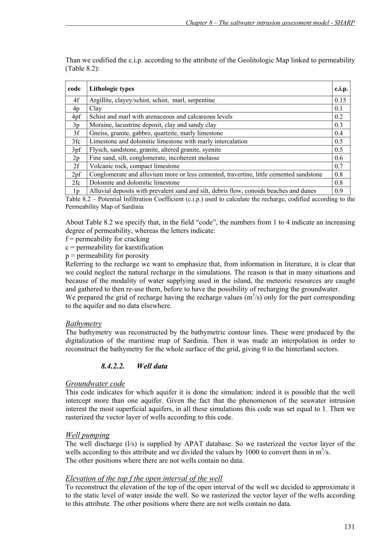
Chapter 8 – The saltwater intrusion assessment model - SHARP
131
Than we codified the c.i.p. according to the attribute of the Geolitologic Map linked to permeability (Table 8.2): code Lithologic types c.i.p.
4f Argillite, clayey/schist, schist, marl, serpentine 0.15 4p Clay 0.1 4pf Schist and marl with arenaceous and calcareous levels 0.2 3p Moraine, lacustrine deposit, clay and sandy clay 0.3 3f Gneiss, granite, gabbro, quartzite, marly limestone 0.4 3fc Limestone and dolomitic limestone with marly intercalation 0.5 3pf Flysch, sandstone, granite, altered granite, syenite 0.5 2p Fine sand, silt, conglomerate, incoherent molasse 0.6 2f Volcanic rock, compact limestone 0.7 2pf Conglomerate and alluvium more or less cemented, travertine, little cemented sandstone 0.8 2fc Dolomite and dolomitic limestone 0.8 1p Alluvial deposits with prevalent sand and silt, debris flow, conoids beaches and dunes 0.9
Table 8.2 – Potential Infiltration Coefficient (c.i.p.) used to calculate the recharge, codified according to the Permeability Map of Sardinia About Table 8.2 we specify that, in the field “code”, the numbers from 1 to 4 indicate an increasing degree of permeability, whereas the letters indicate: f = permeability for cracking c = permeability for karstification p = permeability for porosity Referring to the recharge we want to emphasize that, from information in literature, it is clear that we could neglect the natural recharge in the simulations. The reason is that in many situations and because of the modality of water supplying used in the island, the meteoric resources are caught and gathered to then re-use them, before to have the possibility of recharging the groundwater. We prepared the grid of recharge having the recharge values (m3/s) only for the part corresponding to the aquifer and no data elsewhere. Bathymetry The bathymetry was reconstructed by the bathymetric contour lines. These were produced by the digitalization of the maritime map of Sardinia. Then it was made an interpolation in order to reconstruct the bathymetry for the whole surface of the grid, giving 0 to the hinterland sectors.
8.4.2.2. Well data
Groundwater code This code indicates for which aquifer it is done the simulation: indeed it is possible that the well intercept more than one aquifer. Given the fact that the phenomenon of the seawater intrusion interest the most superficial aquifers, in all these simulations this code was set equal to 1. Then we rasterized the vector layer of wells according to this code. Well pumping The well discharge (l/s) is supplied by APAT database. So we rasterized the vector layer of the wells according to this attribute and we divided the values by 1000 to convert them in m3/s. The other positions where there are not wells contain no data. Elevation of the top f the open interval of the well To reconstruct the elevation of the top of the open interval of the well we decided to approximate it to the static level of water inside the well. So we rasterized the vector layer of the wells according to this attribute. The other positions where there are not wells contain no data.
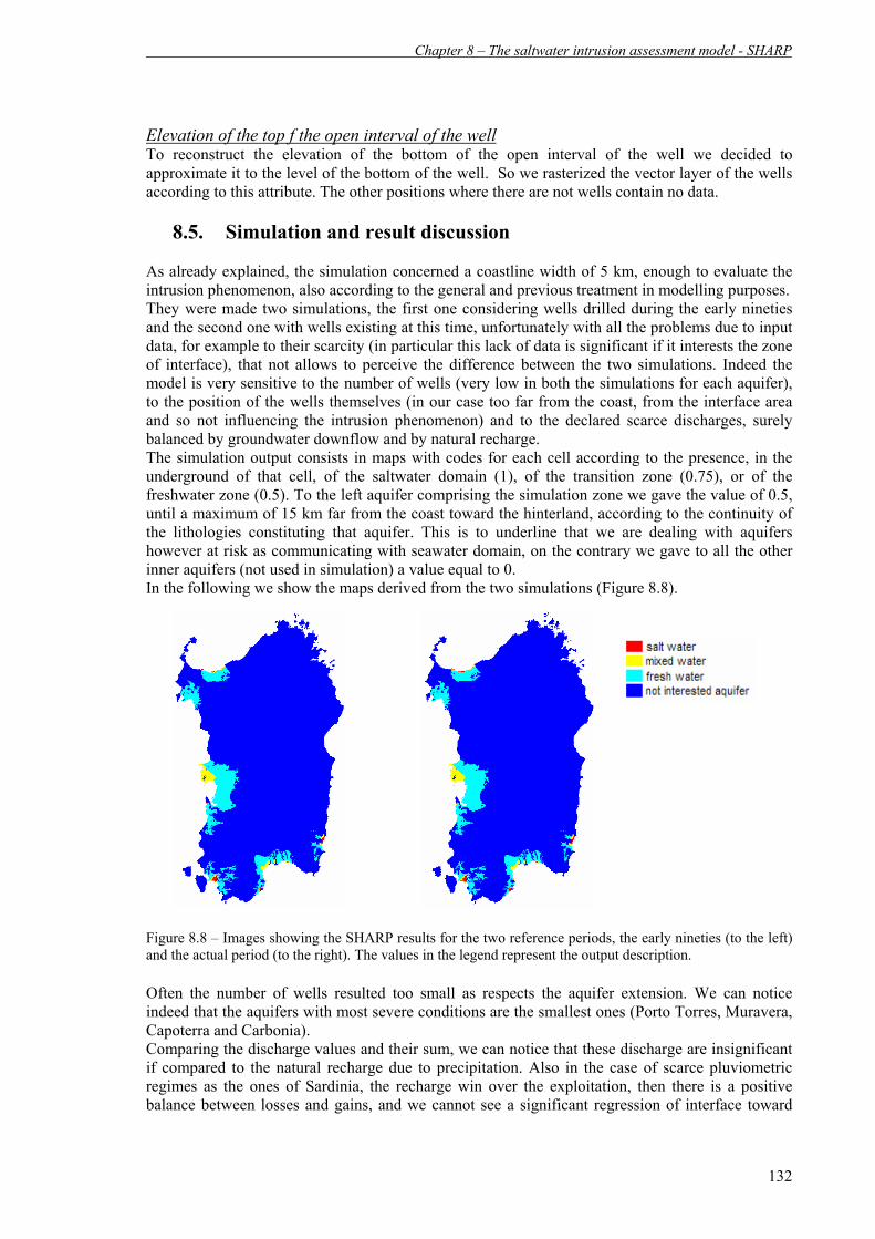
Chapter 8 – The saltwater intrusion assessment model - SHARP
132
Elevation of the top f the open interval of the well To reconstruct the elevation of the bottom of the open interval of the well we decided to approximate it to the level of the bottom of the well. So we rasterized the vector layer of the wells according to this attribute. The other positions where there are not wells contain no data.
8.5. Simulation and result discussion As already explained, the simulation concerned a coastline width of 5 km, enough to evaluate the intrusion phenomenon, also according to the general and previous treatment in modelling purposes. They were made two simulations, the first one considering wells drilled during the early nineties and the second one with wells existing at this time, unfortunately with all the problems due to input data, for example to their scarcity (in particular this lack of data is significant if it interests the zone of interface), that not allows to perceive the difference between the two simulations. Indeed the model is very sensitive to the number of wells (very low in both the simulations for each aquifer), to the position of the wells themselves (in our case too far from the coast, from the interface area and so not influencing the intrusion phenomenon) and to the declared scarce discharges, surely balanced by groundwater downflow and by natural recharge. The simulation output consists in maps with codes for each cell according to the presence, in the underground of that cell, of the saltwater domain (1), of the transition zone (0.75), or of the freshwater zone (0.5). To the left aquifer comprising the simulation zone we gave the value of 0.5, until a maximum of 15 km far from the coast toward the hinterland, according to the continuity of the lithologies constituting that aquifer. This is to underline that we are dealing with aquifers however at risk as communicating with seawater domain, on the contrary we gave to all the other inner aquifers (not used in simulation) a value equal to 0. In the following we show the maps derived from the two simulations (Figure 8.8).
Figure 8.8 – Images showing the SHARP results for the two reference periods, the early nineties (to the left) and the actual period (to the right). The values in the legend represent the output description. Often the number of wells resulted too small as respects the aquifer extension. We can notice indeed that the aquifers with most severe conditions are the smallest ones (Porto Torres, Muravera, Capoterra and Carbonia). Comparing the discharge values and their sum, we can notice that these discharge are insignificant if compared to the natural recharge due to precipitation. Also in the case of scarce pluviometric regimes as the ones of Sardinia, the recharge win over the exploitation, then there is a positive balance between losses and gains, and we cannot see a significant regression of interface toward

Chapter 8 – The saltwater intrusion assessment model - SHARP
133
the hinterland. This is obviously very far from real situation where we know about a overexploitation of the resource. For that concerning the recharge, by test-runs made during the model calibration (see Figure 8.9 about the Muravera aquifer), we noted that the model is very sensitive to the recharge: we made several test-runs excluding the recharge, considering the fact that the possibility of that situation is not far from the reality. Indeed because of the agricultural and irrigation practices in the regions, the precipitation are gathered before recharging the groundwater. This run with zero recharge simulated an evident regression of the interface toward the hinterland as respect the run with recharge, demonstrating that also with a small number of wells, without recharges, the model can simulate the phenomenon.
Figure 8.9 – (Left) Map of bathymetric lines and sketch of Muravera coastal aquifer by satellite (centre). (Top right) results of SHARP simulation considering an high recharge (high precipitation) and (bottom right) results of SHARP simulation considering a null recharge (no precipitation). It is supposed that applying the model over wider temporal scales could highlight major differences at the end of simulation as respects the initial conditions, giving a more important weight to this model, mainly if it will be possible to have more and more detailed input data. Indeed, considering all these uncertainties and imprecision and the sensitivity of the model to some inputs (e.g. the number and position of wells, the pumping and the recharge) we want to underline that for further and more reliable applications they will be necessary many more data and with a detail able to avoid some of difficulties met in the hydrogeological study above described. The model remains an useful tool for further simulation, in particular with most complete datasets in the areas already largely interested by the phenomenon.

PART III
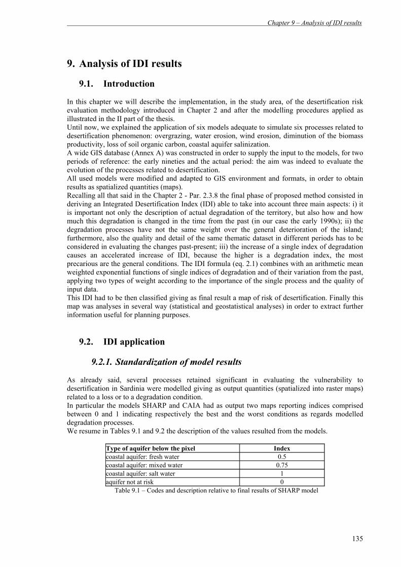
Chapter 9 – Analysis of IDI results
135
9. Analysis of IDI results
9.1. Introduction In this chapter we will describe the implementation, in the study area, of the desertification risk evaluation methodology introduced in Chapter 2 and after the modelling procedures applied as illustrated in the II part of the thesis. Until now, we explained the application of six models adequate to simulate six processes related to desertification phenomenon: overgrazing, water erosion, wind erosion, diminution of the biomass productivity, loss of soil organic carbon, coastal aquifer salinization. A wide GIS database (Annex A) was constructed in order to supply the input to the models, for two periods of reference: the early nineties and the actual period: the aim was indeed to evaluate the evolution of the processes related to desertification. All used models were modified and adapted to GIS environment and formats, in order to obtain results as spatialized quantities (maps). Recalling all that said in the Chapter 2 - Par. 2.3.8 the final phase of proposed method consisted in deriving an Integrated Desertification Index (IDI) able to take into account three main aspects: i) it is important not only the description of actual degradation of the territory, but also how and how much this degradation is changed in the time from the past (in our case the early 1990s); ii) the degradation processes have not the same weight over the general deterioration of the island; furthermore, also the quality and detail of the same thematic dataset in different periods has to be considered in evaluating the changes past-present; iii) the increase of a single index of degradation causes an accelerated increase of IDI, because the higher is a degradation index, the most precarious are the general conditions. The IDI formula (eq. 2.1) combines with an arithmetic mean weighted exponential functions of single indices of degradation and of their variation from the past, applying two types of weight according to the importance of the single process and the quality of input data. This IDI had to be then classified giving as final result a map of risk of desertification. Finally this map was analyses in several way (statistical and geostatistical analyses) in order to extract further information useful for planning purposes.
9.2. IDI application
9.2.1. Standardization of model results As already said, several processes retained significant in evaluating the vulnerability to desertification in Sardinia were modelled giving as output quantities (spatialized into raster maps) related to a loss or to a degradation condition. In particular the models SHARP and CAIA had as output two maps reporting indices comprised between 0 and 1 indicating respectively the best and the worst conditions as regards modelled degradation processes. We resume in Tables 9.1 and 9.2 the description of the values resulted from the models.
Type of aquifer below the pixel Index coastal aquifer: fresh water 0.5 coastal aquifer: mixed water 0.75 coastal aquifer: salt water 1 aquifer not at risk 0
Table 9.1 – Codes and description relative to final results of SHARP model

Chapter 9 – Analysis of IDI results
136
Overgrazing intensity at the pixel Index Very high 1 High 0.75 Medium 0.50 Low 0.25 Very low 0 Unclassified Null
Table 9.2 – Codes and descriptions relative to final results of CAIA model On the contrary the erosion models (WEAM and RUSLE) and the models about productivity (CENTURY and MOD17) had as final output some quantities indicating the erosion amount (t/ha*year) and the productivity (gC/m2*year), respectively. So, in order to derive from these dimensional quantities again indices varying from 0 to 1 in line with the other outputs, we studied a procedure for normalizing them, different for the two types of models (erosion and productivity).
9.2.1.1. Normalization of erosion model results The RUSLE and WEAM models gave as output a quantity indicating a loss of soil due to erosion, expressed as t/ha*year. To normalize this quantity and assign then to each pixel of final map a value ranging from 0 to 1 according to the severity of risk, we decided first to think on a land use basis. For each land use type we had to estimate a value of erosion considered critical: it is clear, indeed, that the same quantity of loss of soil can be more or less severe according to the use of the land in a given territory interested by the erosion process. Moreover, same land uses in different parts of the region can have more comparable values of erosion rather than land uses different one another. In this way it would be possible to say if two areas far-away each other but with the same land use have or not the same vulnerability conditions. For example, normalizing the loss of soil calculated for a cultivated area with the maximum value of erosion found at regional scale and falling, for example, over a very sloped area, bare and not utilized, could lead to an underestimation of the phenomenon where the vulnerability (quantity of loss) is lower, but the risk is higher as we are dealing with a productive area, for which also moderate losses in quantity can be critical. Considering the different detail of the Corine Land Cover datasets for the two periods of reference, we worked for both the outputs of these models getting a re-classification at the third level of the Corine Land Cover itself. Then they were made statistical analyses on a land use basis allowing to derive, for each land use, a statistical descriptive analysis of the distribution of erosion quantities, focusing in particular on: - the mean value of the distribution; - the standard deviation of the distribution; Deeply analyzing the histogram of distribution we decided to consider as critical conditions the ones defined by a value at + 2 standard deviations from the mean (Figure 9.1), that also coincided with a point of natural break (it is a point value that best group similar values and maximize the differences between classes of histogram) for most of the land uses classes.

Chapter 9 – Analysis of IDI results
137
Figure 9.1 – Example of histogram of output values of the RUSLE model, in this case for the broadleaf forest class. As critical value it was chosen the one at + 2 standard deviations from the mean, that often coincide with a break value (blue bar = 11.81) of the natural break algorithm in classifying the histogram. We delete from the histogram the outliers. At this point, given a generic value E of erosion and E2SD the chosen critical value, the following procedure was applied in order to normalize E and to derive an erosion index EI: If E < E2SD then
SDEEEI2
=
else if E ≥ E2SD
1=EI Normalizing according to the maximum of the curve of the histogram, for each land use, could mean underestimate many situations (only one pixel could be at very critical conditions, not excluding that this maximum value could derive by combination of extreme input values due to errors inside the datasets (outliers) and they could not be representative). In our case we considered outliers (errors) the values beyond the 90° percentile. On the contrary normalizing only according to a value distant one standard deviation from the mean could mean to overestimate critical conditions, given the distribution of values. In the Figure 9.2 there is a comparison, for the RUSLE model, among the hotspots resulted by the model output (left, in red) in (t/ha*year), the standard deviation of the distribution resulted from the zonal statistics on a land use basis (centre) and the resulting index after normalizing above described (right). We can notice there was an increase of hotspots, not resulting from previous direct model output.

Chapter 9 – Analysis of IDI results
138
Figure 9.2 – (Left) Erosion map (t/ha·year) resulted from the model simulation; (centre) standard deviation map obtained by a zonal statistics on a land use basis (third level of the CORINE LAND COVER database); (Right): map of the normalized index according to procedure described in the text. All that is for the RUSLE model. The Table 9.3 reports the results of the statistical analysis given on a land use basis for the RUSLE model, listing, for each land use class: the number of pixel interested, the area (in m2), the maximum, the range, the mean, the standard deviation and the critical value according to the choices made to derive it (two times the standard deviation).
CLASS N. PIXEL AREA MAX RANGE MEAN STD CRITICAL
VAL 111 111899 279747000 88.18410 88.18410 0.07677510 1.204580 2.48593510 112 67412 168530000 102.59100 102.59100 0.20638300 1.575180 3.35674300 121 29699 74247500 64.34650 64.34650 0.05586340 0.801880 1.65962340 122 5682 14205000 32.64410 32.64410 0.11732500 1.188920 2.49516500 123 1924 4810000 14.31890 14.31890 0.03119040 0.548574 1.12833840 124 3243 8107500 5.65043 5.65043 0.00503087 0.110202 0.22543487 131 23164 57910000 172.93500 172.93500 0.33281900 3.346480 7.02577900 132 1379 3447500 17.27430 17.27430 0.12130200 1.031080 2.18346200 133 8668 21670000 39.08420 39.08420 0.17332800 1.499960 3.17324800 141 1721 4302500 31.36930 31.36930 0.05369470 0.901035 1.85576470 142 8965 22412500 51.45770 51.45770 0.08373890 0.920864 1.92546690 143 947 2367500 21.69090 21.69090 0.18950100 1.396240 2.98198100 211 1151368 2878420000 214.21100 214.21100 5.01584000 5.842200 16.70024000 212 1405762 3514410000 102.25500 102.25500 2.77679000 4.481740 11.74027000 221 63808 159520000 52.97410 52.97410 2.92231000 3.792770 10.50785000 222 41055 102638000 41.84720 41.84720 1.08633000 2.267660 5.62165000 223 174410 436025000 128.87700 128.87700 4.05965000 5.350070 14.75979000 231 38028 95070000 69.38100 69.38100 4.43283000 5.215610 14.86405000 241 251333 628332000 81.93570 81.93570 4.51769000 5.082640 14.68297000 242 172492 431230000 89.09310 89.09310 3.34247000 4.452200 12.24687000

Chapter 9 – Analysis of IDI results
139
243 109161 272902000 81.32160 81.32160 4.64890000 5.101740 14.85238000 244 202866 507165000 108.27000 108.27000 5.46518000 5.689560 16.84430000 311 1808682 4521700000 469.37400 469.37400 2.27993000 5.167890 12.61571000 312 84291 210728000 212.46700 212.46700 1.75132000 5.427940 12.60720000 313 33107 82767500 99.35810 99.35810 1.84008000 4.475650 10.79138000 321 519734 1299340000 286.66800 286.66800 7.20843000 12.000000 31.20843000 322 59561 148902000 272.83400 272.83400 12.35630000 21.297700 54.95170000 323 2405236 6013090000 330.80000 330.80000 4.62359000 6.965140 18.55387000 324 430269 1075670000 169.91700 169.91700 3.57523000 5.683970 14.94317000 331 11777 29442500 109.90900 109.90900 2.76026000 7.801080 18.36242000 332 32493 81232500 142.65400 142.65400 0.33826800 3.364730 7.06772800 333 251261 628153000 489.58500 489.58500 11.67930000 22.345400 56.37010000 411 5959 14897500 25.65510 25.65510 0.03643320 0.481360 0.99915320 421 12328 30820000 17.17240 17.17240 0.01722940 0.252076 0.52138140 422 19905 49762500 4.96449 4.96449 0.00117476 0.049467 0.10010956 423 249 622500 13.23390 13.23390 0.14443500 1.083750 2.31193500 511 3135 7837500 69.97640 69.97640 0.23148600 2.323880 4.87924600 512 38717 96792500 142.13300 142.13300 0.08314520 1.591410 3.26596520 521 30305 75762500 9.34078 9.34078 0.00429804 0.119475 0.24324804 522 243 607500 1.55517 1.55517 0.02405150 0.172777 0.36960550 523 62 155000 0.00000 0.00000 0.00000000 0.000000 0.00000000
Table 9.3 – Statistics of erosion values of RUSLE made over the third level (first column) of the Corine Land Cover database. The critical value is considered the one far +2 standard deviations from the mean. We want to underline that the critical values for several land use classes, derived by statistical analyses over the value distribution on a land use class basis, well reflect some values reported in literature even for the Sardinia region by numerous studies (e.g. Vacca et al., 2000). For example, one of these studies carried out over different land use (e.g. Santa Lucia River at the south of the island) shows critical values of erosion comprised between 2 and 12 t/ha*year. The threshold values extracted for the same type of land use (Eucalyptus) show values with the same order of magnitude. It is evident, speaking about not precise values but of order of magnitude, that using a critical value of 200 t/ha*year for erosion (as suggested by FAO/UNEP/UNESCO, 1979), could have underestimate largely the phenomenon in that area. Further, in particular for agricultural areas, the critical values (with a mean of about 13 t/ha*year) obtained by normalization methodology, are very similar, at least for the order of magnitude, to those reported in literature (Øygarden et al., 2003), according to the following classification (where we assumed the very high risk as the critical condition):
1. Low (<0.5 t/ha) 2. Medium (0.5-2 t/ha) 3. High (2-8 t/ha) 4. Very high (>8 t/ha)
At the end, both for RUSLE and for WEAM, the normalized index was then classified in the following way (Table 9.4), matching the one chosen for the IDI and explained below (Par. 9.3).
Description of Erosion Risk Index 5 – Very high 0.7 – 1 4 – High 0.5 – 0.7 3 – Medium 0.3 – 0.5 2 – Low 0.15 – 0.3 1 – Very low 0.0 – 0.15
Table 9.4 – Table showing the classification of the erosion risk values.

Chapter 9 – Analysis of IDI results
140
To compare each other the classified indices between the two periods, it was decided first of all to use an aggregating algorithm to evaluate jointly maps at 250 meters of resolution in order to overcome the difference in detail between the datasets of two periods. In the aggregation algorithm we took into account the maximum value of the pixel, this because even the presence of a single pixel belonging to the class of higher risk had to be considered however critical. The resulting maps for RUSLE model (Figure 9.3) show, besides a light “shift” of the areas at “risk” between the two periods toward the centre of the island, the remaining of critical conditions in areas that will be interesting in the analysis of final output (see later).
Figure 9.3 – Spatialization of classified erosion indices for the RUSLE model, for the early nineties period (left) and the actual period (right) Following map in Figure 9.4 shows, still for RUSLE model, the areas at risk with the meaning of areas where both there is actually a risk condition (class 3 or 4 or 5), both where there has been a worsening in respect to the past.
Risk

Chapter 9 – Analysis of IDI results
141
Figure 9.4 – Map showing as critical the areas that both suffered from a worsening in respect to the past and have now an erosion risk from medium (class 3) to very high (class 5). In particular the percent distribution analysis of the risk classes (Table 9.5) shows that, at a resolution of 250 meters, there was an increase of the total areas interested by the sum of classes 3-4-5: from the 55.4% of the early nineties to 58.4% of the actual period.
Table 9.5 – Distribution (%) of the water erosion risk classes for the past period (left) and the actual one (right)
9.2.1.2. Normalization of productivity model results The productivity models CENTURY and MOD17 gave as output the annual carbon productivity (gC/m2*year) for the soil and the vegetation, respectively. To normalize this quantity and assign then to each pixel of the final map a value ranging from 0 to 1 according to the severity of risk, we decided first to think on a homogeneous territorial unit basis and not only on a land use basis. These homogeneous units area are characterized not only by the same land use, but also by the same range of minimum temperatures and precipitations, the two variables that can determine a situation more or less critical inside the same land use for the productivity, even as seen by the sensitivity of models. For each one of these homogeneous units was then necessary to derive a value of productivity considered critical: we can indeed guess that a same value can be more or less critical according to the use of land in the territory and to the micro-climate to which it is typically exposed. Taking into account the different detail of the CORINE LAND COVER layer for the two periods of reference, we worked for the CENTURY model with a reclassification to the third level, while for the MOD17 we reclassified the land use according to the macro-classes already used for the downscaling (Table 5.4).
PAST RISK % 1 26.68006 2 17.94848 3 16.46923 4 11.17993 5 27.7223
ACTUAL RISK % 1 21.63634 2 19.96818 3 19.59111 4 13.11044 5 25.69393

Chapter 9 – Analysis of IDI results
142
The map of the annual mean of minimum temperatures was reclassified into four classes: 1-4°C, 4-8°C, 8-12°C, 12-16°C according to an equal interval; the map of annual mean of precipitations was classified in this way: 0-410 mm, 410-580 mm, 580-750 mm, 750-920 mm according to a breakpoint method. From the combination of these two layers with the one of land use it was derived a map reporting the homogeneous units to use in the normalization procedures (Figure 9.5).
Figure 9.5 - Map of precipitation classes (a), temperature classes (b) and reclassified land use (c) used to define homogeneous units (d) over which to made statistical analyses to normalize the output of MOD17 model. We made then some statistics on the basis of homogeneous units allowing to derive in particular, for each unit: - the mean of distribution; - the standard deviation of distribution;
at this point we considered as alarming conditions for the productivity the ones defined by a value far -1 standard deviation from the mean, after a careful examination of curve of distribution, also if critical values often considered at global scale are lower. At this point, given a generic value of productivity P and the critical value PSD, the following procedure was applied in order to normalize P and to derive an erosion index PI: If P > PSD then
PP
PI SD=
else if P ≤ PSD
1=PI Normalizing according to the absolute minimum of the histogram (in general 0) could mean to underestimate most of the situations (only one pixel should be at very critical conditions, not excluding that this minimum values could derive by combination of extreme input values due to errors inside the datasets that cannot be representative).

Chapter 9 – Analysis of IDI results
143
In Figure 9.6 there is a comparison between the hotspots (left, in red) resulted by the CENTURY output (gC/m2*year), the mean of the distribution (gC/m2*year) resulted by a zonal statistics on a homogeneous unit basis (centre) and the resulting index after the normalization above described (right). We can notice there was a large increase of hotspots that did not result from direct model output.
Figure 9.6 – CENTURY model results: (Left) Soil productivity map (gC/m2*year) resulted from the model simulation; (centre) map of the means obtained by a zonal statistics on a homogeneous unit basis as explained in the text; (Right): map of the normalized index according to procedure described in the text. Both for CENTURY and for MOD17, the normalized index we then classified in the following way (Table 9.6), matching the one chosen for the IDI and explained below (Par. 9.3).
Description of Productivity Loss Risk Index 5 – Very high 0.7 – 1 4 – High 0.5 – 0.7 3 – Medium 0.3 – 0.5 2 – Low 0.15 – 0.3 1 – Very low 0.0 – 0.15
Table 9.6 – Table showing the classification of the loss of productivity risk values. In comparing each other the classified indices between the two years for the productivity models, it was decided first of all to use an aggregating algorithm in order to evaluate jointly maps at 250 meters of resolution to overcome the difference in detail between the datasets of two periods. Also in this case (par 9.2.1.1), in the aggregation algorithm we took into account the maximum value of the pixel. Making the difference between the classified indices for the two years (Figure 9.7), it is highlighted a situation more or less stable over the two years of reference, with very few hotspots or brightspots referring to improved or worsened areas. All that suggests for both the periods a situation however delicate for the vegetation in general, (probably related to climatic regime consisting in high temperatures and low precipitations), but without an accelerated trend toward the worst situations.

Chapter 9 – Analysis of IDI results
144
Figure 9.7 – Map of the differences of indices between the actual situation and the past one, after re-aggregating the output at 250 meters of resolution.
9.2.2. Weighting the indices According to the previous operations and the IDI formula, there are twelve grids of input for the final desertification index computation: the first six for the results obtained by simulation models of the actual periods, the last six for the results derived by simulation models of the past period. Then they are necessary the grids of reclassified land uses, of the minimum temperatures and of the mean precipitations, all useful in normalizing procedures above described. For each process, the indices relative to actual period and to early nineties years derive from the same model, but the input dataset is characterized by some unhomogeneities for that concerning the detail and the resolution (first of all the land use layer, a fundamental input for all the models and mainly for the downscaling procedure, that for the actual period has a scale of 1:25’000, for the past period has a scale of 100’000). Moreover, the processes have not the same influence over the desertification phenomenon: some of them are significant, other ones are less important, all that according to an expert knowledge of the territory and according to past studies. Besides the grids of model results they were introduced in the IDI formula some weights for the normalized indices and for the variations of normalized indices between the two periods of simulation. In particular we gave a lower weight to the indices variation ∆ID because of the different detail of the two sets of data and, in the case of the MOD17 model, also because the lack of an original MODIS datum for the early nineties period that was derived synthetically through calibration with the images of another sensor (AVHRR, see Chapter 5 – Par. 5.3). We made a series of evaluations to avoid, for example, that a model less reliable than another influenced too much the final result, taking anyway into account that the performances, at this time, of the single models as applied in this study, are proportional to the influence of single processes over the desertification phenomenon.

Chapter 9 – Analysis of IDI results
145
Further, assuming that used models have a valid scientific support and documented validation experiments, nevertheless this could be not enough: a model scientifically valid but with a poor quality of inputs cannot give good results. In these situations are often the models simpler and less sophisticated to give satisfying results (e.g., RUSLE, CAIA). Indeed, considering other factors as the complexity of simulated process and the major or minor reliability of the model for the study area, we gave a decreasing weight from CAIA and RUSLE, to MOD17, to CENTURY, to WEAM, to SHARP. Then, to consider the importance and the complexity of models and the quality of inputs, we made following assumptions:
- the CAIA model is studied over the territory of Sardinia and then it is strongly reliable. Anyway we decided to give a lower weight to the difference between the two periods because of the difference in detail of input data (e.g. the land use layer);
- the RUSLE model is very simple, it doesn’t require sophisticated operations and furthermore it is well tested for every type of land use, also in two dimensions and into a GIS environment: fort his reason it can be considered a good estimator, also considering the big work of choice and refining of inputs. For that concerning the two runs, we have to recognize that the input data have different resolution (for example NDVI, see Chapter 3 – Par. 3.4.6);
- the MOD17 model refers to remote sensed data, the nearest to the reality. Despite this added value to modelling approach, we needed a downscaling procedure that forced us to give a lower weight to this model as regards the two previous models. Considering the difference between the detail of data for the runs of the two years, also in this case it is the land use to play a fundamental role;
- the CENTURY model is a very complex model and sophisticated in its procedures and having a very strong scientific support, but for this reason it results to be more delicate in input choice: for that we gave a lower weight to this model as regards the MOD17. For that concerning the differences between two years, also in this case we had to consider the difference in resolution among the inputs.
- The WEAM model is a semi-empirical model. Nevertheless there are several inputs, as the roughness vegetation to which the model is sensible, whose preparation is very difficult and also in the scientific field it is still an open issue. For the spatial attribution of this parameter, as well as in the downscaling of LAI, again the detail differences among the inputs of the two periods suggest to differently weight the indices.
- The SHARP model is a very complex model, that considers very sophisticated physical processes, and then it was very delicate in input preparation activity. Indeed the simulation resulted affected by the poor quality and scarcity of input data. So we gave a very low weight to this model and to variation of its indices.
We resume in the Table 9.10 the final weights given to the indices and their variations:
Table 9.10 – Chosen weights to give to indices and their variation in the IDI calculation
MODELS Weights CAIA 1.00 variation_CAIA 0.25 RUSLE 1.00 variation _RUSLE 0.25 MOD17 0.80 variation _MOD17 0.20 CENTURY 0.60 variation _CENTURY 0.15 WEAM 0.40 variation _WEAM 0.10 SHARP 0.20 variation _SHARP 0.05
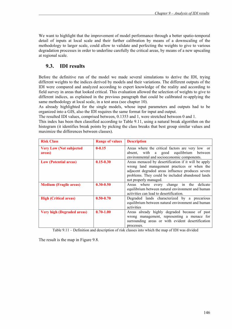
Chapter 9 – Analysis of IDI results
146
We want to highlight that the improvement of model performance through a better spatio-temporal detail of inputs at local scale and their further calibration by means of a downscaling of the methodology to larger scale, could allow to validate and perfecting the weights to give to various degradation processes in order to underline carefully the critical areas, by means of a new upscaling at regional scale.
9.3. IDI results Before the definitive run of the model we made several simulations to derive the IDI, trying different weights to the indices derived by models and their variations. The different outputs of the IDI were compared and analyzed according to expert knowledge of the reality and according to field survey in areas that looked critical. This evaluation allowed the selection of weights to give to different indices, as explained in the previous paragraph that could be calibrated re-applying the same methodology at local scale, in a test area (see chapter 10). As already highlighted for the single models, whose input parameters and outputs had to be organized into a GIS, also the IDI requires the same format for input and output. The resulted IDI values, comprised between, 0.1353 and 1, were stretched between 0 and 1. This index has been then classified according to Table 9.11, using a natural break algorithm on the histogram (it identifies break points by picking the class breaks that best group similar values and maximize the differences between classes).
Risk Class Range of values Description
Very Low (Not subjected areas)
0-0.15 Areas where the critical factors are very low or absent, with a good equilibrium between environmental and socioeconomic components.
Low (Potential areas) 0.15-0.30 Areas menaced by desertification if it will be apply wrong land management practices or when the adjacent degraded areas influence produces severe problems. They could be included abandoned lands not properly managed.
Medium (Fragile areas) 0.30-0.50 Areas where every change in the delicate equilibrium between natural environment and human activities can lead to desertification.
High (Critical areas) 0.50-0.70 Degraded lands characterized by a precarious equilibrium between natural environment and human activities
Very high (Degraded areas) 0.70-1.00 Areas already highly degraded because of past wrong management, representing a menace for surrounding areas or with evident desertification processes.
Table 9.11 – Definition and description of risk classes into which the map of IDI was divided The result is the map in Figure 9.8.

Legendnull or very low risk
low risk
medium risk
high risk
very high risk
not applicable
1:1000000scale
Figure 9.8 - Map of reclassifed IDI as explained in the text
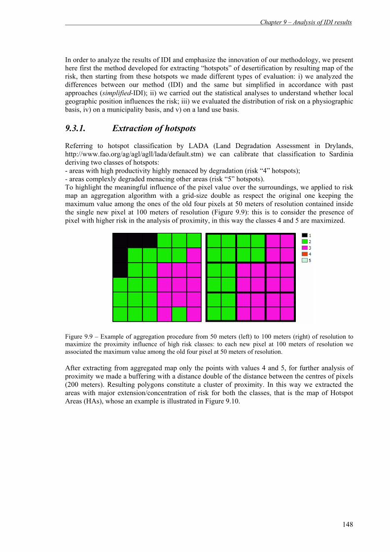
Chapter 9 – Analysis of IDI results
148
In order to analyze the results of IDI and emphasize the innovation of our methodology, we present here first the method developed for extracting “hotspots” of desertification by resulting map of the risk, then starting from these hotspots we made different types of evaluation: i) we analyzed the differences between our method (IDI) and the same but simplified in accordance with past approaches (simplified-IDI); ii) we carried out the statistical analyses to understand whether local geographic position influences the risk; iii) we evaluated the distribution of risk on a physiographic basis, iv) on a municipality basis, and v) on a land use basis. 9.3.1. Extraction of hotspots Referring to hotspot classification by LADA (Land Degradation Assessment in Drylands, http://www.fao.org/ag/agl/agll/lada/default.stm) we can calibrate that classification to Sardinia deriving two classes of hotspots: - areas with high productivity highly menaced by degradation (risk “4” hotspots); - areas complexly degraded menacing other areas (risk “5” hotspots). To highlight the meaningful influence of the pixel value over the surroundings, we applied to risk map an aggregation algorithm with a grid-size double as respect the original one keeping the maximum value among the ones of the old four pixels at 50 meters of resolution contained inside the single new pixel at 100 meters of resolution (Figure 9.9): this is to consider the presence of pixel with higher risk in the analysis of proximity, in this way the classes 4 and 5 are maximized.
Figure 9.9 – Example of aggregation procedure from 50 meters (left) to 100 meters (right) of resolution to maximize the proximity influence of high risk classes: to each new pixel at 100 meters of resolution we associated the maximum value among the old four pixel at 50 meters of resolution. After extracting from aggregated map only the points with values 4 and 5, for further analysis of proximity we made a buffering with a distance double of the distance between the centres of pixels (200 meters). Resulting polygons constitute a cluster of proximity. In this way we extracted the areas with major extension/concentration of risk for both the classes, that is the map of Hotspot Areas (HAs), whose an example is illustrated in Figure 9.10.

Chapter 9 – Analysis of IDI results
149
Figure 9.10 – Procedure for proximity analysis to extract Hotspot Areas (HAs). Left: northwest part of Sardinia with location of pixels at risk 4 and 5 according to the classification in Table 9.11; Top right: zoom to an area with high concentration of pixels at risk; Bottom right: result of proximity analysis (aggregation, buffering) as described in the text. Starting from extraction of these HAs, we made a series of analyses below described. 9.3.2. Comparison of IDI with a simplified-IDI First we compared two cases deriving from two runs of the model: a) a simplified-IDI, consisting in using no weights for the evaluated processes, that is considering all the processes have the same influence on the territory (PIDi=1 in eq. 2.1) and considering only the present situation (P∆IDi=0 in eq. 2.1, that is equal to consider no change from the past); and b) an IDI, consisting in using degradation indices derived applying models for the two periods (early nineties and surrounding of actual period) and giving decreasing weights to processes according to classification in Table 9.10. In the case b) it is also given a lower weight to “variation” of indices ∆IDi (see eq. 2.1) between the two periods as regards the weight given to indices IDi because of differences in the detail of input data (in this example, for all the processes, P∆IDi =0.25 PIDi, as shown in Table 9.10). In Table 9.12 we compared the differences in surface of HAs for the two approaches, showing how the consideration or not of past situation, of the detail and quality of input data and of the expert-team judgment in indicating the most influencing processes leads to a great difference in outputs: IDI estimates 16% of the territory as hotspots of risk, whereas the simplified-IDI estimate the 31%.
Case Hotspots 4 (Ha) Hotspots 5 (Ha) Hotspot 4 % Hotspot 5 % Total %
Simplified-IDI 644351 105180 26.75 4.37 31.12
IDI 358994 35850 14.90 1.49 16.39
Table 9.12 – Resulting areas in Hectares and in percent of the total island surface for each type of HAs both for Simplified-IDI and IDI, as explained in the text. Field inspections (see below) in these HAs to validate the results suggested that the IDI satisfactorily detect them, whereas simplified-IDI tends to overestimate the risk.

Chapter 9 – Analysis of IDI results
150
9.3.3. Field verification The IDI results were verified during a field survey made in the weeks from December 4th – 7th, 2006 and May 8th – 11th 2007. The following Figure 9.11 shows the location of the municipalities whose territory was deeply visited.
Figure 9.11 – Areas of Sardinia deeply investigated during the field survey carried out in order to validate the IDI results. The verification was made jointly with experts of University of Sassari mainly in the areas resulted at high risk (HAs) from IDI computation. In the following Figure 9.12 they are reported particulars of the visited areas highlighting the municipality comprising the territory surveyed.
Figure 9.12 – Zoom from Figure 9.11 in areas interested by deep field validation, highlighting their municipality boundaries.

Chapter 9 – Analysis of IDI results
151
The field validation confirmed the results of the IDI, in particular that the larger contribution to desertification is due to overgrazing management and soil erosion combination, causing very precarious conditions in these areas. Table 9.13 and Figure 9.13, show the location and the environmental description of checked areas and an example of the severe situation for the Irgoli site (north-eastern part of the island), respectively. SITE LON LAT HAs Description
s1 9.032 39.446 4 Agricultural area with several signs of rill incision s2 9.046 39.475 no Agricultural area without sign of degradation
s3 9.053 39.511 5 Area lacking of vegetation cover, devoted to grazing, sloped and with signs of grazing amelioration procedures
s4 9.039 39.582 4 Agricultural areas surrounded by highly grazed area s5 8.920 39.567 no Signs of ploughing on gently sloped areas, deep soil without stoniness s6 8.959 39.598 no Signs of ploughing on gently sloped areas, deep soil without stoniness s7 9.025 39.635 4 Sloped ploughed areas s8 8.931 39.656 no Signs of ploughing on gently sloped areas, deep soil without stoniness s9
9.244
40.313
5
Sloped area with alternation of schlerophyllus vegetation and bare/grass cover, showing signs of irregular land-work often in the direction of slope for pasture seeding, also signs of rill/sheet erosion.
s10 9.456 40.419 4 s11 9.467 40.461 4
Sparsely vegetated (shrubs) and very sloped areas with diffuse sign of ploughing in the direction of slope, some sing of rill/sheet erosion
s12 9.654 40.454 4 s13 9.693 40.476 5 s14 9.704 40.480 4
Land interested by grazing, with sparse or low vegetation (shrubs), degraded soil with high stoniness, with deep incision due to rill erosion, up to outcropping of mother rock.
s15 8.670 40.533 4 s16 8.628 40.600 4 s17 8.563 40.607 5 s18 8.485 40.660 4
Areas devoted to grazing and intensive and extensive agriculture
s19 8.471 40.743 no s20 8.639 40.741 no s21 8.289 40.746 no
Agricultural land, with gently slope, without signs of degradation
s22 8.194 40.735 4 Agricultural areas also devoted to grazing, with medium slope s23 8.204 40.781 4 Agricultural areas also devoted to intense grazing, with high slope s24 8.243 40.831 no Agricultural areas also devoted to grazing, with medium slope
Table 9.13 - Codifying, location (longitude and latitude, in decimal degrees) of checked sites, report of the type of HAs resulting form the hotspot analysis, if present, and description of the real conditions detected during the survey.

Chapter 9 – Analysis of IDI results
152
Figure 9.13 – (Top left) Field survey points (yellow triangles) and road map (red line); (Left) Example of superimposition of HA limits (red line) over an aerial photograph in a surveyed location resulting as a hotspot: it resulted a grazed area with evident erosion phenomena (top right) leading to total loss of soil and to the outcropping of rock (bottom right). (Field survey, December 2006). At this point, in order to extract the map of Macro Hotspots Areas (MHAs) for case b), with the aim of bounding wider zones with a more delicate equilibrium, we carried out an analysis of clustering of HAs by means of an hotspot analysis procedure (Getis-Ord Gi* statistics, implemented into ArcGIS software) that tells us whether and where features with high values (risk 5) or features with low values (risk 4) tend to cluster in the study area, looking at each feature within the context of neighbouring features and weighting this clustering tendency by means of a Z-score (Ebdon, 1985), that represents the statistical significance of clustering. For statistically significant positive Z-Scores, the larger the Z-score is, the more intense the clustering of high values. For statistically significant negative Z-scores, the smaller the Z-Score is, the more intense the clustering of low values. In our case the chosen significance level was 0.05, then we extracted polygons with Z-scores ≥ 2 to emphasize the MHAs of class 5. Results showed two large MHAs and three smaller MHAs given by a high concentration (clustering) of hotspots of class 5 (Figure 9.14).

Chapter 9 – Analysis of IDI results
153
Figure 9.14 – Macro Hotspot Areas (MHAs) of class 5 (in black) extracted by clustering analysis of previous Hotspot Areas (HAs) for case b), as explained in the text, dark grey areas refer to clustering of classes 4, light grey areas represent no significant clustering. Further, the two hugest MHAs confirm two large critical areas detected by a previous work at regional scale (Motroni et al., 2004, see Fig. 2.9). In successive analyses we took into account only the IDI results.
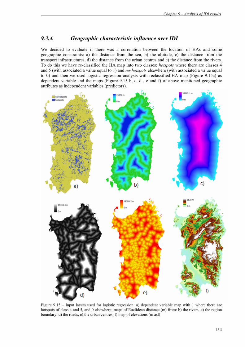
Chapter 9 – Analysis of IDI results
154
9.3.4. Geographic characteristic influence over IDI We decided to evaluate if there was a correlation between the location of HAs and some geographic constraints: a) the distance from the sea, b) the altitude, c) the distance from the transport infrastructures, d) the distance from the urban centres and e) the distance from the rivers. To do this we have re-classified the HA map into two classes: hotspots where there are classes 4 and 5 (with associated a value equal to 1) and no-hotspots elsewhere (with associated a value equal to 0) and then we used logistic regression analysis with reclassified-HA map (Figure 9.15a) as dependent variable and the maps (Figure 9.15 b, c, d , e and f) of above mentioned geographic attributes as independent variables (predictors).
Figure 9.15 – Input layers used for logistic regression: a) dependent variable map with 1 where there are hotspots of class 4 and 5, and 0 elsewhere; maps of Euclidean distance (m) from: b) the rivers, c) the region boundary, d) the roads, e) the urban centres; f) map of elevations (m asl)

Chapter 9 – Analysis of IDI results
155
Results of logistic regression analysis are coefficients describing the weight that a predictor has over the presence/absence of the risk in a map unit. From the analysis (logistic regression) of spatial relationship between these geographic characteristics (predictors) and the distribution of highest risk classes (HAs at risk 4 and 5), no significant influence for all the considered predictors was found, suggesting that desertification has not preference for particular “isolation/accessibility” conditions and confirming that the phenomenon is very complex and not reducible only to geographic attributes (predisposing factors). 9.3.5. Risk evaluation on a basin scale Hydrographic basins represent territorial units adequate for analysis of environmental variables, as naturally constituted by physiographic units well defined and for which it is possible to evaluate independently the erosion/deposition processes, previously acknowledged (Chapter 2 – Par. 2.2.2) as a primary factor of desertification in Sardinia. After extracting the main basins of the island from the specific dataset (http://www.clc2000.sinanet.apat.it/cartanetms/), we calculated the extent of the surface occupied by each type of HAs (class 4 and 5) inside each basin, highlighting the ones interested by wider risk. Results (Table 9.14 and Figure 9.16) showed that the north-western basins (Mannu, Coghinas and Temo river basins) together with the Flumendosa river basin in the central-eastern part of the island are the most affected: in all these basins the area at risk is at least one fourth of the total surface. These are indeed the basins with high cattle loading and presenting morphology and lithology favouring the erosion.
BASIN NAME Hotspot risk
4 (Ha) Hotspot
risk 5 (Ha) BASIN
AREA (Ha) % Hotspot
risk 4 % Hotspot
risk 5 0 - Liscia 3276 317 56710 5.78 0.56 1 - Coghinas 55363 5503 248151 22.31 2.22 2 - Padrogiano 3342 112 44968 7.43 0.25 3 - Mannu di Porto Torres 18717 1850 66877 27.99 2.77 4 - Barca 5532 138 35353 15.65 0.39 5 - E Posada 12438 895 69684 17.85 1.28 6 - Tirso 64038 3865 350619 18.26 1.10 7 - Temo 20385 1495 83730 24.35 1.79 8 - Cedrino 24149 1939 108945 22.17 1.78 9 - Rio di Mare Foghe 3854 120 42518 9.06 0.28 10 - Flumendosa 40114 6679 186792 21.48 3.58 11 - Mannu 21759 1154 171915 12.66 0.67 12 - Mogoro 2013 19 58417 3.45 0.03 13 - Durci 3465 398 37549 9.23 1.06 14 - Mannu 3636 287 59255 6.14 0.48 15 - Sa Picocca 4393 302 39190 11.21 0.77 16 - Cixerri 5903 620 57568 10.25 1.08 17 - Palmas 4271 337 47752 8.94 0.71
Table 9.14 – HAs evaluation on a basin scale. Code-name of the basins (first column), area (in hectares) of HAs at risk 4 (second column) and 5 (third column), basin area in hectares (fourth column), percent of HAs at risk 4 (fifth column) and 5 (sixth column). The numbers in the first column are the same reported in Figure 9.16.

Chapter 9 – Analysis of IDI results
156
Figure 9.16 – Hotspot analysis on a basin scale. Percent of area covered by HAs for each basin of the island: the numbers recall the code of basins in the first column of Table 9.14. The most affected basins are the ones of Rio Mannu (30.8%), Temo (26.1%), Flumendosa (25%) and Coghinas (24.5%) rivers. 9.3.6. Risk evaluation on a municipality scale We made the same type of analysis above illustrated considering the smallest administrative units, the municipalities, in order to detect the ones whose land is more prone to desertification. The distribution of HAs in this case (Figure 9.17) seems to reflect the two largest MHAs above described (see Figure 9.14), suggesting an interaction of natural conditions and local management and policies in determining the fragility of areas.

Chapter 9 – Analysis of IDI results
157
Figure 9.17 – Hotspot analysis on a municipality scale. Percent of area covered by HAs for each municipality of the island: the most affected sectors are the ones in the north-western part and in the central-south-eastern part of the island. This result is comparable with a socio-economic analysis, still on a municipality scale (Idda and Pulina, 2006, unpublished), made taking into account several indicators as population density, poverty, land use, agricultural/environmental management, infrastructures and land ownership to evaluate a socio-economic risk of desertification. These indicators are operated by means of a geometric mean and the result (an index ranging from -2 to 3.5) individuated the central/south-eastern sectors as the most fragile. After stretching this social risk from 0 to 1 and classifying it in the same categories defined in Table 9.11, its overlay (sum) with classified mean IDI on a municipality basis shows where the two types of risk combine and interact giving the most precarious and severe conditions, that is still in the central/south-eastern sectors. Result of overlay in Figure 9.18 show where the two risk are minimum (value 2) ad where there is the worst combination (value 8), that is where the two risks range in the classes from medium to very high risk (3, 4, 5). It is worth to note that the municipalities with most highly severe conditions are aggregated inside the central-eastern MHAs. So mainly in this sector, besides the menace due to the diffuse presence of HAs at risk 5 in the proximities, there are precarious socio-economic situations, interacting with environmental conditions in a cause-effect relationship.
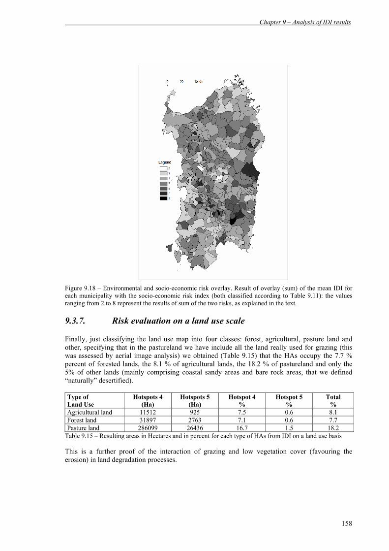
Chapter 9 – Analysis of IDI results
158
Figure 9.18 – Environmental and socio-economic risk overlay. Result of overlay (sum) of the mean IDI for each municipality with the socio-economic risk index (both classified according to Table 9.11): the values ranging from 2 to 8 represent the results of sum of the two risks, as explained in the text. 9.3.7. Risk evaluation on a land use scale Finally, just classifying the land use map into four classes: forest, agricultural, pasture land and other, specifying that in the pastureland we have include all the land really used for grazing (this was assessed by aerial image analysis) we obtained (Table 9.15) that the HAs occupy the 7.7 % percent of forested lands, the 8.1 % of agricultural lands, the 18.2 % of pastureland and only the 5% of other lands (mainly comprising coastal sandy areas and bare rock areas, that we defined “naturally” desertified). Type of Land Use
Hotspots 4 (Ha)
Hotspots 5 (Ha)
Hotspot 4 %
Hotspot 5 %
Total %
Agricultural land 11512 925 7.5 0.6 8.1 Forest land 31897 2763 7.1 0.6 7.7 Pasture land 286099 26436 16.7 1.5 18.2
Table 9.15 – Resulting areas in Hectares and in percent for each type of HAs from IDI on a land use basis This is a further proof of the interaction of grazing and low vegetation cover (favouring the erosion) in land degradation processes.

Chapter 10 – Methodology application at lager scale: “partial-IDI”
159
10. Methodology application at larger scale: ”partial-IDI”
10.1. Introduction
In the Chapter 9 we showed the methodology for extracting the Hotspot Areas for the classes of risk 4 and 5 and we did an analysis of distribution of these areas on different bases: hydrographic basins, municipalities, land use. In this chapter we applied the developed methodology to a test area in order to better calibrate the whole procedure. The selection of the test area, according to the driving forces more representative of the desertification, was made mainly on the basis of an integrated analysis of following factors:
1. Concentration of high and very high risk pixels, according to the geostatistical evaluation of territorial data;
2. Identification of areas morphologically and physiographically homogeneous, to evaluate dynamics of erosion phenomena, influent over the degradation of the island;
3. Representativeness according to processes determining desertification in Sardinia. In the following paragraphs we describe the test area and the application of the methodology to this area, specifying first that given the distance to the sea of the chosen area, in this case the SHARP model was not applied. Then we want to highlight that in this case we applied only the “assessment” part of the IDI formula (actual period) as we were not able to collect data more detailed for the early nineties period, for which we had already used the data with the best detail available in the regional application.
10.2. Test area: Rio Mannu
Starting from the analysis on a physiographic basis described in Chapter 9 Par. 9.3.5, a basin at high risk degree (Figure 10.1) was extracted in order to re-apply the procedure after gathering more detailed data by field campaign.
Figure 10.1 - (Left) Hotspot areas distribution (fraction of surface) on a basin basis, numbers below the diagram show a basin identifier for the most critical basins; (Right) Extracted basin and Hotspot Area (risk 4 and 5) spatial distribution.
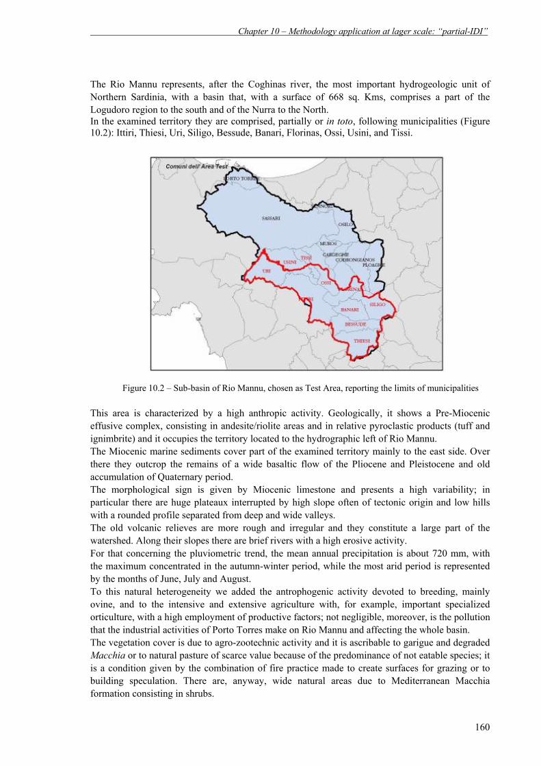
Chapter 10 – Methodology application at lager scale: “partial-IDI”
160
The Rio Mannu represents, after the Coghinas river, the most important hydrogeologic unit of Northern Sardinia, with a basin that, with a surface of 668 sq. Kms, comprises a part of the Logudoro region to the south and of the Nurra to the North. In the examined territory they are comprised, partially or in toto, following municipalities (Figure 10.2): Ittiri, Thiesi, Uri, Siligo, Bessude, Banari, Florinas, Ossi, Usini, and Tissi.
Figure 10.2 – Sub-basin of Rio Mannu, chosen as Test Area, reporting the limits of municipalities
This area is characterized by a high anthropic activity. Geologically, it shows a Pre-Miocenic effusive complex, consisting in andesite/riolite areas and in relative pyroclastic products (tuff and ignimbrite) and it occupies the territory located to the hydrographic left of Rio Mannu. The Miocenic marine sediments cover part of the examined territory mainly to the east side. Over there they outcrop the remains of a wide basaltic flow of the Pliocene and Pleistocene and old accumulation of Quaternary period. The morphological sign is given by Miocenic limestone and presents a high variability; in particular there are huge plateaux interrupted by high slope often of tectonic origin and low hills with a rounded profile separated from deep and wide valleys. The old volcanic relieves are more rough and irregular and they constitute a large part of the watershed. Along their slopes there are brief rivers with a high erosive activity. For that concerning the pluviometric trend, the mean annual precipitation is about 720 mm, with the maximum concentrated in the autumn-winter period, while the most arid period is represented by the months of June, July and August. To this natural heterogeneity we added the antrophogenic activity devoted to breeding, mainly ovine, and to the intensive and extensive agriculture with, for example, important specialized orticulture, with a high employment of productive factors; not negligible, moreover, is the pollution that the industrial activities of Porto Torres make on Rio Mannu and affecting the whole basin. The vegetation cover is due to agro-zootechnic activity and it is ascribable to garigue and degraded Macchia or to natural pasture of scarce value because of the predominance of not eatable species; it is a condition given by the combination of fire practice made to create surfaces for grazing or to building speculation. There are, anyway, wide natural areas due to Mediterranean Macchia formation consisting in shrubs.

Chapter 10 – Methodology application at lager scale: “partial-IDI”
161
The characteristic quality of selected area and the diversification of geomorphology and of impacts over the territory, seem valid assumptions to consider the area well representative of the regional reality and, then, adequate for the verification and tuning of produced regional output.
10.3. New input production
The resolution for the modelling of considered test area passed from 50 meters to 25 meters, then it was necessary the acquisition of more detailed data (in particular for that concerning the Pedologic Map through field survey) or the derivation of them from datasets at coarser resolution, that will be described below.
10.3.1. Pedologic Map
The Pedologic Map at finer resolution was elaborated referring to following parameters useful as inputs: - Rockiness; - Superficial stoniness; - Drainage; - Soil depth; - Texture; - Available Water Content; - Soil organic matter - Soil organic carbon - Field capacity - cm H2O per cm of soil - Wilting point - cm H2O per cm of soil
For the sampling activities, the Rio Mannu area was divided in a grid of 450 cells of about 50 hectares, whose the centroids were considered. Of these 450 points 400 descriptive points were chosen and 150 of these points were sampled (Figure 10.3) by experts of the University of Sassari and analyzed to extract parameters necessary to elaborate the inputs of the models.
Figure 10.3 – Map of the sampling grid and of point whose pedologic characteristics were analyzed.

Chapter 10 – Methodology application at lager scale: “partial-IDI”
162
10.3.2. Updating of the Land Use map The land use map Corine Land Cover 2003 was updated through field survey at the time of field sampling and photo interpretation analysis made over ortophotos. They have been detected land use boundaries and updated the limits of pedologic formations with the aim of producing a more detailed map.
10.3.3. Precipitation data
For the inputs relative to monthly precipitation, necessary for RUSLE and CENTURY models, they have been used the data from 417 meteo stations, supplied by the Regional Administration (referring to the period 1982-2003), whose location is shown in Figure 10.4.
Figure 10.4 – Distribution of meteorological stations reporting the monthly precipitation data for the period 1982-2003.
The data were in tabular format and report the monthly precipitation (mm) for each measurements station, to which we associated the latitude/longitude coordinates. To produce grids containing surface with the spatialized datum of monthly precipitation we applied the kriging interpolation technique contained into the toolset Interpolation of the Spatial Analyst toolbox of ArcGIS. For this aim we selected several stations both inside and outside (in the surrounding of) the test area (Table 10.1):
Villanova Monteleone Reinamare (C.ra) Ittiri Putifigari Rudas (C.ra) Olmedo F.C. Chiesi Bidighinzu-Diga (C.M.)Uri Plaghe Cargeghe Osilo Sassari (Genio Civile) Torralba FF.SS. Ardara Romana Bancali
Table 10.1 – Stations used to interpolate precipitation data in the Test Area

Chapter 10 – Methodology application at lager scale: “partial-IDI”
163
10.3.4. Normalization Difference Vegetation Index
We acquired a set of remote sensed data by ASTER (Advanced Spaceborne Thermal Emission and Reflection Radiometer, see Annex A) sensor, data from which to derive some indices linked to vegetation. The RUSLE and WEAM model application inside the test area required indeed the elaboration of NDVI and LAI, respectively, and their spatialization at 25 meters of resolution. Moreover from NDVI it is possible to derive the FPAR through empirical relationships existing in literature. These indices will be derived from analysis of remote sensed products ASTER, that, in terms of radiometric resolution, spatial and spectral, represent an adequate tool for vegetation analysis in small areas. The following images (Table 10.2) were acquired for the test area (given the variable satellite orbit in some cases it was necessary to acquire two adjacent scenes to cover exactly the area of interest for a given date).
DATE IMAGE NAME CLOUD COVER PERCENT 13/06/04 AST_L1A.003:2024369836 15% 13/06/04 AST_L1A.003:2024369828 14% 03/10/04 AST_L1A.003:2026058390 0% 03/10/04 AST_L1A.003:2026058392 0% 22/12/04 AST_L1A.003:2027138357 21% 22/12/04 AST_L1A.003:2027138382 30% 12/08/05 AST_L1A.003:2030439284 0% 31/03/06 AST_L1A.003:2033719485 0% 31/03/06 AST_L1A.003:2033719489 0%
Table 10.2 – Date, name and characteristics of acquired ASTER images
10.3.5. Digital Elevation Model (DEM) For that concerning the Digital Elevation Model (DEM), both direct and indirect inputs of some models, the Regional Administration supplied a layer at 10 meters of resolution for the area of interest. The DEM was obtained using the spot heights of a Triangulated Irregular Network (TIN) together with the contour lines. With successive elaborations, through the interpolation, it was obtained a regular mesh of points (GRID) with a resolution of 10 meters. Given the resolution for the application in the test area (25 m) this grid was re-sampled from 10 to 25 meters of resolution and used as input to the models. For the re-sampling we applied the BILINEAR technique. We preferred to use this DEM rather the one by IGMI at 25 meters of resolution as starting from a finer detail, also if re-sampled, this allowed to remedy to errors (i.e. pits, flat areas) in general present and due to interpolation methodology for the contour lines and spot heights.
10.4. Application of the models to test-area
10.4.1. RUSLE For the RUSLE model, besides acquiring of detailed data for NDVI computation, we modified the procedures for preparing some data, in particular the ones necessary for the R factor (rain erosivity) and the C factor (vegetation cover). To calculate the erosivity index R (MJ.mm.ha-1h-1y-1) for the test areas we considered directly the monthly precipitations and we used the Arnoldus (1980) method and the Fournier (1960) Index, the

Chapter 10 – Methodology application at lager scale: “partial-IDI”
164
most used in literature and then with an adequate validation support: these maps were directly used as input for the R factor of the RUSLE, as in the case of regional application. For the vegetation cover factor C, in this case, as we needed a finer detail, we used the ASTER products allowing to derive the NDVI at 15 meters of resolution. After georeferencing and mosaicing of images, if necessary, we derived the NDVI from the ratio:
rir
rirNDVIρρρρ
+−
=
where ρir represents the reflectance of the band of the near infrared (0.78 - 0.86 µm), while ρr the one of the red band (0.63 - 0.69 µm). The use of an index consisting in a band ratio allowed also to remedy to the problem of shadow, indeed the two bands are almost affected in the same way by the minor reflectance of wave, then rationing them it is possible to simplify the effect on both the bands. At this point the NDVI images at 15 meter of resolution were derived and then they were re-sampled to 25 meters of resolution, each one representative of a season. The relationship between the C factor and NDVI is the same applied to the regional scale that is the following (Knijff et al., 2000):
⎟⎠⎞
⎜⎝⎛−
=NDVINDVIC
15.2exp
For the left inputs, they were prepared in the same way than for the regional application and consisted in:
- updating of land use for the data regarding the features of the landscape limiting the runoff, to calculate the combined LS and P factors;
- using of Pedologic Map for the content of soil organic matter, the structure, the texture, the drainage capacity, all playing a role in calculation of K factor.
The model run in the Rio Mannu area produced quantities of erosion ranging from 0 (non-erodible areas) to 516.77 t/ha*year. Comparing the erosion map (Figure 10.5) with the DEM we can evince the highest values are more concentrated on steepest hillslope areas, along the river incisions.
Figure 10.5 – RUSLE results for the RIO MANNU sub-basin

Chapter 10 – Methodology application at lager scale: “partial-IDI”
165
Then we analyzed the model results according to four classes of elevations, four classes of slope and eight classes of exposition. The elevation classes were divided according to the natural break technique, the classes are based over groups better maximizing the differences among the classes. The breaks are put where there are the higher “jumps” in the value distribution. The classes were: 1 (blue): 41.12 -227 m asl 2 (green): 227 – 361 m asl 3 (light blue): 361 – 481.26 m asl 4 (red): 481.26 -738.24 m asl In the Figure 10.6 we can see that, analyzing the distribution of erosion values according to the elevation class, the differences among the averages are not to evident (ranging from 22. 2 to about 29.2 t/ha*year).
Figure 10.6 – Averages of erosion values for each elevation class
Also the slope values were divided in classes according to the natural break, the classes were: 1 (blue): 0 – 7.4° 2 (green): 7.4 – 15.05° 3 (light blue): 15.05 – 24.13° 4 (red): 24.13 - 60.93° In the Figure 10.7 we can see that, analyzing the distribution of erosion values according to the slope class, the differences among the means are very evident, with erosion values increasing with the increase of slope, highlighting the high sensitivity of the RUSLE model to the LS factor.
Figure 10.7 – Averages of erosion values for each slope class

Chapter 10 – Methodology application at lager scale: “partial-IDI”
166
The aspect classes were divided according to the technique of the equal interval: The classes were: 1 (blue): Flat areas 2 (light green): North 3 (light blue): North East 4 (red): East 5 (pink): South East 6 (yellow): South 7 (dark blue): South West 8 (dark green): West 9 (dark cyan): North West In the following Figure 10.8 we can see, analyzing the distribution of erosion values for each exposition class, the erosion values increase for aspects toward the south. The reason of this can be that the soils toward the south are the most fragile because they are exposed to frequent episodes of drying and imbibitions.
Figure 10.8 – Averages of erosion values for each aspect class The analysis of the distribution of the average values according to the land uses classes (at the third level of the Corine Land Cover database) shows very high values for the grazed areas and the areas with sparse vegetation (Figure 10.9).

Chapter 10 – Methodology application at lager scale: “partial-IDI”
167
Figure 10.9 – Averages of erosion values for each land use class (third level of the Corine Land Cover database, see legend in Annex A for the description of the classes) Comparing the regional output at 50 meters of resolution and this one at 25 meters for this area, we can notice that, assuming as more reliable the output at 25 meters of resolution, the values at 50 meters of resolution are underestimated in the most sloped areas, this is because the model is highly sensible to the slope through the LS factor. In the Figure 10.10 we reported this comparison where we can note the correspondence between the sloped areas (visible in Figure 10.10a from the hillshade model of DEM) and the negative values (light yellow) in the Figure 10.10b, corresponding to situations where in the regional result there is an underestimation as regards the local result.

Chapter 10 – Methodology application at lager scale: “partial-IDI”
168
Figure 10.10 – a) DEM hillshade in the Rio Mannu test area; b) differences between the model output quantities for the run at 50 meters of resolution and the one at 25 meters. In the following Figure 10.11 we report the distribution of the classified index for the results with two resolutions, showing as the detail difference can cause a different percent of areas at low or high risk.
Figure 10.11 – Comparison of the distribution of classified index for the two simulations, both for the test area We can notice that, considering the outputs with finer detail as the most reliable, the “regional” application overestimate the high risk (classes 4 and 5), with a percent cover varying from 29% (at 50 metres of resolution) to 18% (at 25 meters of resolution). Finally we made a comparison on the spatial correspondence of those classified indices, considering a subdivision in high risk (classes 4 and 5) and medium-low risk (classes 1-2-3) categories. In the Figure 10.12 below we report the map showing in red the areas where there is not matching of the two categories between the two resolutions, while in green areas there is correspondence. We highlight that the distribution pattern follow the same of Figure 10.10b.

Chapter 10 – Methodology application at lager scale: “partial-IDI”
169
Figure 10.12 – Comparison of the correspondence of the high risk classes (4 and 5) and medium-low (1, 2 and 3) in the two runs with different detail: the red areas indicate where the response is different, the green ones where the response is the same.
10.4.2. WEAM For that concerning the WEAM model, we made some modification for the preparation of the seasonal LAI to estimate the vegetation cover fraction protecting the soil from wind erosion. In particular we started from the seasonal NDVI derived from the ASTER images. The used relationship to derive first the cover fraction Cf was derived from the one of (Knijff et al., 2000):
( )( )NDVINDVIf eC −−−= 15.21
Then the seasonal LAI as derived inverting the relationship of Choudhury (1989):
( )21*100 LAIf eC −−=
Assuming random distribution of foliage above the soil and uniform leaf-angle distribution. The left inputs were prepared at the same way than at the regional scale application:
• updating the land use for the inputs regarding the roughness and the drag coefficient of vegetation;
• using the Pedologic Map for the texture of soil. For that concerning the meteorological data (Mean Temperatures, Dew Point Temperatures, Wind speed), on the contrary, we resampled to 25 meters the data used for regional scale application. As we could imagine, given the location of the test area in the inner part of the island, the wind regimes are not enough to cause wind erosion, because of a “topographic barrier” against a phenomenon that is however of low influence for the whole island. The output of this model was negligible.

Chapter 10 – Methodology application at lager scale: “partial-IDI”
170
10.4.3. MOD17 For the model MOD17 only one modification in the application was made, regarding the production of the FPAR data (with an 8-days synthesis) to use in calculation of the GPP. Starting from the seasonal images of NDVI derived from ASTER (Par. 10.3.4), we derived a seasonal FPAR, according to the relationship (Chang and Wetzel 1991): FPAR = 1.5 (NDVI - 0.1) NDVI ≤ 0.547 FPAR = 3.2 (NDVI) - 1.08 NDVI > 0.547 Then we calculated the ratios between the images of FPAR at 25 meters of resolution obtained for the 4 seasonal images (dates) of ASTER and the ones of FPAR at 50 meters of resolution relative to the same date (see Chapter. 5). Then these “seasonal” ratios (at 25 meters of resolution) were multiplied by the other FPAR images at 50 meters of resolution, each ratio according to the correspondent season of image. Finally we obtained 46 images of FPAR at 25 meters constituting the model inputs for the MOD17. For the left inputs, they were prepared as for the regional application: - updating the land use useful for the ε data (radiation use efficiency) and for the parameters regarding the scalar factors of minimum Temperatures and of Pressure Vapour Deficit. For that concerning the meteorological data (Minimum Temperatures, Vapour Pressure Deficit, Short Wave Radiation) they have been re-sampled to 25 meters the data used for the regional application. The model run produced following results (Figure 10.13) showing a good correspondence with the results at 50 meters of resolution, that it is clear also looking at the minimum and maximum reported in the legend and also at the statistics of distribution.
Figure 10.13 – Outputs of the MOD17 model for the test area at 25 (top) and 50 (bottom) meters of resolution.

Chapter 10 – Methodology application at lager scale: “partial-IDI”
171
This correspondence reflected well also in normalized and classified index percent distribution both on a land use class basis and considering the whole test area territory.
10.4.4. CENTURY
For that concerning the CENTURY model, some modifications for the test area regarded the precipitation datasets. For the monthly data, we used the measurements of the 417 stations from 1982 to 2003 ( Par. 10.3.3) having a more detail than the dataset used at regional scale. So the grids derived by interpolation (12 grids for each of 22 years) were averaged obtaining a grid for each month, from which we then extracted the means for each polygon where we ran the model. For the left inputs, we prepared them at the same way than for the regional application:
- updating land use for the new overlays with the Map Sheets (Chapter 6, Par. 6.3); - using the Pedologic Map for the textural data, the field capacity, the wilting point, the
organic carbon and the organic matter. For that concerning the other meteorological data (Mean monthly minimum temperature, Mean monthly Maximum Temperature and standard deviation of Precipitation) on the contrary, they have been simply re-sampled to 25 meters the data used at regional scale. For the CENTURY model we want to underline that, in the two runs at different resolutions, the results of normalized indices are similar, there are only changes from the class 4 to the class 5 or viceversa. The two thirds of the classes that suffered from modifications between the two runs are relative to the agricultural areas. In the Figure 10.14 we can see the map reporting in grey the areas with the same result between the two runs, and in blue the areas with different results that, anyway, consists for the 95% of cases in 1 class of difference.
Figure 10.14 – Map showing the areas where the two classified outputs (at 25 and at 50 meters) are the same (grey) and the areas where the two outputs are different (blue).

Chapter 10 – Methodology application at lager scale: “partial-IDI”
172
10.4.5. CAIA
For the model CAIA, some modifications were made to the input data: in particular the vegetation cover data (from Corine Land Cover database) were updated delimiting the grazed areas through photointerpretation and field survey. The value of actual CAIA was defined according to the zootechnical data on a Map Sheets (Annex A) basis in the study area, then this vector layer was converted to a grid with 25 meters of resolution, representing the informatic layer of actual CAIA. For the sustainable CAIA, the input data derived from pedologic information and from field sampling and successive analyses. By means of geostatistical techniques (co-kriging) these parameters were spatialized: rockiness, depth, stoniness and fertility. During the field campaign it was also possible to validate the actual CAIA results for the application at regional scale. As shown in the Figure 10.15 and in Table 10.3, the model output shows that the 35% of the grazed territory in interested by overgrazing phenomena, given by the fact that the animal loading remains in a continuous manner over the same domain the whole year. In this way there are not “rest periods” for the grazing allowing the grazing sustainability.
Figure 10.15 – Output of the CAIA model in the test AREA
OUTPUT SURFACE (ha) SURFACE (%) 0 1239.5 7.4
0.25 3702.4 22.0 0.50 3336.0 19.8 0.75 2710.2 16.1
1 5870.8 34.8 Table 10.3 – Percent distribution of the CAIA index in the test area

Chapter 10 – Methodology application at lager scale: “partial-IDI”
173
Some areas are at the same time used for the agriculture and for the grazing, negatively impacting over the territory (e.g. the areas of Ossi e Ittiri, where the overgrazing causes also erosion phenomena and compacting of soil, in this areas the CAIA values was about 1). In most cases the vulnerability can be ascribed to geomorphology (steep slopes and stoniness), low fertility of areas devoted to grazing, favouring the water erosion. According to the soil survey we can then confirm that the evaluation of impact of overgrazing is coherent with the CAIA results for the different typologies of territory. The results of the CAIA model are coincident for the two applications at different resolution, also if there are some local differences. In some areas falling inside the municipalities of Ittiri, Banari e Bessude there are some differences but the error relative to the study at regional scale remained inside 1 class, this is obviously due to more detailed input data. Then, the methodology used to evaluate the areas with “overgrazing” risk seemed adequate for the aim, considering that the regional results will be improved when there will be at one’s disposal detailed data for the whole regional territory.
10.5. Partial-IDI After running the IDI only for the part relative to actual conditions (partial-IDI) and with the same weights given for the previous regional application, we made a field validation on the test areas confirming the ability of the developed tool to detect areas at different risk of desertification. We show here a comparison between the results of two applications: the former at 25 meters of resolution (Figure 10.16) and the latter extracted by the regional application 50 meters of resolution, but only for the actual period (Figure 10.17).
Figure 10.16 - Reclassified output for the test Area (partial-IDI), for the run at 25 meters of resolution.

Chapter 10 – Methodology application at lager scale: “partial-IDI”
174
Figure 10.17 - Reclassified output for the test Area (partial IDI), for the run at 50 meters of resolution
We can notice the general distribution of hotspots remains the same, but it is accentuated in the run at 25 meters, mainly in the Southern part. In general we can highlight a diminution of “risk 4” areas and an increase of “risk 3” areas. In the Figure 10.18 below the green areas represent the areas were the output was the same, whereas the red areas represent the areas where the results were different.
Figure 10.18 - Map showing the distribution of areas where there are no differences of results between the two applications (green), and the areas where there are differences (red). Anyway all the variations remain inside one class, as we can see in the following Figure 10.19, representing the distribution, in number of pixels, of the differences between the two applications.

Chapter 10 – Methodology application at lager scale: “partial-IDI”
175
Figure 10.19 - Distribution (in number of pixels) of the differences between the two applications of Partial-IDI at different resolutions. The Rio Mannu area can be confirmed as an area with a delicate equilibrium and with precarious conditions, in particular we can highlight a new hotspot to the south of area and other ones sparse in the territory and due in particular to the better detail of inputs of the models regarding the two most important processes: overgrazing and water erosion.

Chapter 11 – Future scenarios of desertification
176
11. Future scenarios of desertification
11.1. Introduction
In the past two centuries the impact of human activities on the land has grown exponentially, changing entire landscapes, impacting the soils, the hydrological cycles and the climate and leading in some cases to desertification. The underlying driving forces of land use changes can be recognized as a multitude of economic, technological, institutional, cultural and demographic factors. With the aim of dealing with land use change predictions for environmental management, models are a very useful tool. Indeed by means of scenarios they allow to identify future land use location inside the environmental changes. The aim of the work reported in this Chapter was to evaluate desertification risk scenarios taking into account both bio-physical and socio-economic factors, and using the well developed CLUE-s model (Verburg et al., 2002) to supply different scenarios of probable land use changes for the future, driven both by climate changes (according to climate predictions for the end of this century) and by evaluation of plausible human needs. The power of this model is the possibility to make all the simulations one wants supposing, for example, different policies and regulations for the future. The island conditions of Sardinia favour the use of this model as this territory can be considered, for certain aspects, as a close system. In the next paragraphs we will introduce the model and the choices made for its application in the study area, we will give details about the whole methodology and its implementation and we extracted finally the results for two applications of the model at regional scale considering two different demand scenarios.
11.2. Modelling of land use change
11.2.1. CLUE-s model With CLUE model (Velkamp and Fresco, 1996), in contrast to other empirical models of land use changes, it is possible to simulate multiple land-use types simultaneously through the dynamic simulation of competition between land-use types. As CLUE model considers mixed pixels, that is a pixel can be occupied by different fractions of land use, and taking into account the extent of our study area, we chose to use the modified modelling approach for our applications of the model, that is CLUE-s (the Conversion of Land Use and its Effects at Small regional extent) version (Verburg et al., 2002). In the following we will illustrate the main concepts over which CLUE-s scheme is based and its structure.
11.2.1.1. Main Principles
As already said, land-use and land-cover changes are the result of many interacting processes. These processes can be driven by several variables influencing the actions of the involved agents of land-use and cover change. These driving factors often include demographic factors (e.g., population increase and pressure), economic, technological, policy, institutional, social, cultural factors, and last but not least biophysical factors (Turner II et al., 1995; Kaimowitz and Angelsen, 1998). All these factors influence land-use change in different ways: directly and indirectly. Further they can influence either the rate or the velocity of land use change or determine the location of land-use change. As the driving forces are highly variables in space and time, it is necessary to take into account all those drivers related to the same period in starting analyses of land use change and it is important to

Chapter 11 – Future scenarios of desertification
177
consider their spatial variability: especially for factors that are significant in determining the location of change it is essential that these factors can be spatialized. Other properties relevant for land use systems are stability and resilience, concepts referring to the ability of the ecosystem or society to adapt themselves to perturbations, or the magnitude of disturbance that can be tolerated before a system changes its structure (Holling, 1992).
11.2.1.2. Driving factors
The economists model the relation between the location factors and land use assuming that, in equilibrium, land is devoted to the use that generates the highest potential profitability, reflected in land rents. Social factors influence location choices of households, whose determinants are cultural values, norms and preferences (lifestyles) of individuals and their financial, temporal, and transport means. Policies at national or sub-national level have influence on land use. In particular, policies that have a spatial manifestation (for example, the creation of protected areas) influence the spatial pattern of land-use change. The CLUE-s model allows the incorporation of a large number of factors important for land-use change derived from the different disciplinary understandings. We want to specify that CLUE-s permits to consider not only static driving factors, that are the driving factors not changing during simulation, but also some dynamic driving factors: in this case the predictors are supposed changing during simulation according to time-related datasets.
11.2.1.3. Model Description
The CLUE-S model can be divided into two modules, a module of non-spatial demand and a module of allocation spatially explicit (Figure 11.1). In the non-spatial demand module the changes in land use are estimated for a series of years at the aggregate level, only as total quantities in the study area, without considering the location of these changes.
Figure 11.1 Non-spatial and spatial modules on which CLUE-s model is based (from Engelsman, 2002).
To assess the land-use demand it is possible to extrapolate trends in land use change from the past into the future and, when necessary, these trends can be corrected for changes in population growth and/or diminishing land resources. For policy analysis it is also possible to base land use demands on advanced models of macro-economic changes, which can serve to provide scenario conditions as consequence of policy decisions.
DRIVING FACTOR ACTUAL LAND USE
LOGISTIC REGRESSION
PROBABILITY FOR ALL
CHANGES IN DRIVING
ALLOCATION
AREA RESTRICTION
CONVERSION STABILITY
Spatial Non spatial
DEMAND OF ALL LAND USE TYPES

Chapter 11 – Future scenarios of desertification
178
The choice for one of the models depends mainly on the availability of input data. The results of the demand module is the area (in Ha, created for every time step considered in the simulation) covered by the different land use types and it is used as direct input for the spatial module of the CLUE-s model. Land use conversions are expected to take place at locations with the highest 'preference' for the specific type of land use at that moment in time. The spatial module has to translate the changes in demand into changes in land use pattern within the study region using a raster-based system. If the simulation comprehends several years, for every year of simulation a land use prediction map can be created. To work, the allocation module needs decision rules and the results of a statistical analysis as input, indicating together the potential locations for conversion. Then the model allocates these demands for land-use conversions at specific locations within the study area. Figure 11.2 gives an overview of the procedure.
Figure 11.2 - Schematic representation of the procedure to allocate changes in land use to a raster based map. The empirical analysis clarifies the relationships between the spatial distribution of land use and a series of factors that are drivers and constraints of land use. The results of this empirical analysis are used within the model when simulating the competition between land-use types for a specific location. In addition, a set of decision rules is specified by the user to restrict the conversions that can take place based on the actual land-use pattern and to specific policies.
11.2.1.4. Spatial Analysis
The pattern of land use reflects the spatial organization of land use in relation to the underlying biophysical and socio-economic conditions. Apart from land use, it is necessary to gather data representing the driving forces assumed at the basis of land use in the study area. The list of assumed driving forces is based both over literature (Lambin et al., 2001; Kaimowitz and Angelsen 1998; Turner II et al., 1993) and/or knowledge of the specific conditions in the study area. Data can originate from remote sensing (e.g., land use, elevation), secondary statistics (e.g., population distribution), maps (e.g., soil, vegetation), and other sources. To allow a straightforward analysis, the data are converted into a grid based system with a cell size that depends on the finer and most frequent resolution of the available data. The relations between land use and chosen driving factors are thereafter evaluated using stepwise logistic regression. Logistic regression is an often used methodology in land-use change research (e.g. Geoghegan et al., 2001; Serneels and Lambin, 2001). In this model logistic regression is used to indicate the probability of a certain grid cell to be devoted to a land-use type given a set of driving factors.
Driving factors Actual Land Use
Logistic Regression
Probability for each Land Use
Elasticity to conversion
Allocation Demand
Competition
Decision Rules
Chapter 11 – Future scenarios of desertification
179
Logistic regression calculates the occurrence of an event, using the independent variables as predictor values. This method is used when a dependent is a dichotomy (0 or 1) and the independents are continuous variables or categorical variables (Garson, 2002). In this study, logistic regression equation, for each land use, is
(11.1)
where Pi is the probability of a grid cell for the occurrence of the considered land-use type and the x are the driving factors. By means of logistic regression it is possible to select the most relevant driving factors from an initial larger set of factors that are assumed to influence the land-use pattern. This choice is made according to the value of beta coefficients, showing the degree of influence of driving factor over the dependent variable. Finally, variables that result with no significant contribution to explain land-use pattern (β≈0) are excluded from the final regression equation. By the results of the regression, probability maps can be calculated for each land use and for every year of the simulation: it is possible to take into account also the updated values of the driving factors that are changing in time (e.g. population density, climate). Logistic regression produces odds ratios associated with each predictor value. These ratios are the exponents of the logit coefficient and therefore also called the exponent of β (Exp (β)). The odds of an event represent the probability of the event occurring divided by the probability of the event not occurring. The odds ratio for a predictor tells the relative amount by which the odds of the outcome increase (odds ratio > 1) or decrease (odds ratio < 1) when the value of the predictor value is increased by 1 unit. Because all independents have different units it is not possible to immediately find the most important variable in the model. Because of the impossibility to compare the different Exp (β) of the driving factors with each other, the relatively influence can be calculated. This is called the odds max ratio. This odds max ratio is calculated by taking the Exp (β) of the non-categorical driving factors and their total range. Relative influence = Exp (β * range) for exp(β) > 1 Relative influence = -1/ Exp (β * range) for exp(β) < 1 The goodness of fit for the logistic regression can be evaluated with the ‘Relative Operating Characteristics’ (ROC) method (Pontius and Schneider, 2000) which evaluates the predicted probabilities by comparing them with the observed values. The accuracy of the model is measured in area beneath the ROC-curve. The values differ from 0.5 to 1, with 0.5 if the model does not predict the changes any better than a random approach. If the value is 1 the discrimination is perfect.
11.2.1.5. Decision rules
Decision Rules for land use type allocation can be specified by the user, there are three types of decision rules:
• spatial policies, delineating protected areas such as nature reserves or national parks or all areas where no changes can be allowed;
• for each land-use type they exist the conditions under which the land-use type is allowed to change in the next time step. These decision rules are implemented to give to each land-use type a certain resistance (or reversibility) to change in order to generate the stability in the land-use structure that is typical for many landscapes. Different situation can be described by the relative elasticity for change (ELASu) for the land-use type into any other land use type. The relative elasticity ranges between 0 and 1, the higher the defined elasticity, the more difficult it gets to convert this land-use type. There are also land use types that operate in between these two extremes. This situation is representative for the land use types that are not likely to change after their first establishment. But it is clear that on the long term, when there is a land use type that is more profitable, the land use will change.
nni
i xxxxP
P⋅++⋅+⋅+⋅+=⎟⎟
⎠
⎞⎜⎜⎝
⎛−
βββββ ...1
log 3322110
Chapter 11 – Future scenarios of desertification
180
The stability settings are based on the knowledge of the experts about the location or observed behaviour in the recent past. The settings can also be tuned during the calibration of the model;
• it is necessary to consider the possibility to convert or not a land use type into another (for example is unlikely that urban use will be converted into forest use).
11.2.1.6. Allocation
Competition and actual allocation of land-use change are made in an iterative procedure given the probability maps, the decision rules in combination with the actual land-use map and the demand for the different land-use types. In the allocation module the demand of the different land use types form each year is spatially allocated. This allocation procedure (Figure 11.3) follows four steps (Verburg et al., 2001):
1. the number of grid cells that have to be taken into account in the allocation are counted, whereas the grid cells that are either part of a protected area or not allowed to change for another reason are excluded from further calculations;
2. for all grid cells i the total probability for each land use u (TPROPi,u) is calculated. The total probability is calculated according to the following equation: TPROPi,u = Pi,u + ELASu + ITERu (11.2) where Pi,u is the probability derived by logistic regression, ITERu is an iteration variable that is specific of the land use, ELASu is the relative elasticity for change specified in the decision rules and is only given a value if grid cell i is already under land use type u in the year considered, ELASu equals zero if all changes are allowed;
3. a preliminary allocation is made with an equal iteration variable ITERu for each land use type. In this step the land use type with the highest probability is allocated in the considered grid cell;
4. the total allocated area of the different land use types is now compared to the demand. If the number of allocated grid cells of a certain land use type is too high, the iteration variable is decreased. If the number of allocated grid cells is too low compared to the demand, the iteration variable is increased. Within the iterative procedure there is a continuous interaction between macro-scale demands and local land-use suitability as determined by the regression equations. Instead of only being determined by the local conditions, captured by the logistic regressions, it is also the regional demand that affects the actually allocated changes. This allows the model to “override” the local suitability: it is not always the land-use type with the highest probability according to the logistic regression equation (Pi,u) that is allocated into the grid cell;
The steps 2 to 4 are repeated until the allocated land use matches with the demand within the convergence criteria specified by user (that had to select the maximum deviation allowed for a land use and the mean deviation allowed considering all the land uses). When the allocation matches the demand the final result is saved. Now the model can proceed to the next time step (usually years). If convergence is not reached into 20000 iterations, the model is assumed have no solutions.

Chapter 11 – Future scenarios of desertification
181
Figure 11.3 – CLUE-s allocation scheme. Representation of the iterative procedure for land use change allocation (modified from Verburg et al., 2004) until the satisfaction of demands and of convergence criteria.
11.2.1.7. Model limits
Actual version of the model has some limits we took into account in preparing simulation and in making decisions about input data: the model is able to work with a maximum of 15 land use classes and 30 driving factors, and the maximum size of grids is 2500x2500 pixels.
11.3. CLUE-s implementation in the study area To describe the CLUE-s model application carried out to simulate land use changes in Sardinia, we will explain in this paragraph following steps, resumed in Figure 11.4:
• it was necessary to collect all data about the study area considered useful to implement the methodology, that is to collect the land use and the predictor variables layers;
• the data were homogeneneized in order to respect the same reference system, resolution and spatial extent;
• the collected data were analyzed statistically together with the information of actual land use;
• we prepared all the input data needed for simulation: aggregate demands of land use and maps of independent (driving factors) and dependent (land use) variables;
• we prepared some scenarios of changes taking into account most important climate parameters and socio-economic variables;
• we made different simulations, adjusting and varying some model parameters according to the performance required by model.

Chapter 11 – Future scenarios of desertification
182
Figure 11.4 – Flow chart of the structure of the simulation made by the model (from Engelsman, 2002).
11.3.1. Driving factors
All used data were clipped according to the administrative limit of Sardinia region. All the input data, spatialized or not, had to be imported into GIS format (GRID structure) and homogenized (e.g. the Reference System and the Resolution had to be the same: the datum was World Geodetic System WGS84, the Projection was UTM - Universal Transverse Mercator, zone 32 N), in order to allow an easy implementation of the procedure, to make all the necessary analyses and overlays among different layers and information and to supply the results with the same structure. As already said, changes in land use pattern can be caused by a number of different factors. These factors are called driving factors of land use change. After several attempts in choosing the driving factors for adequately running the model we selected the most adequate ones, so in the following we will describe in detail the used dataset and the operation made on them. All driving factor data were derived from datasets that already existed. All data were thoroughly checked and updated. The chosen final resolution of this data set was a 100-meter grid, so the surface of one grid cell was 1 Ha. In particular we chose to work with 12 driving factors falling into different categories: socio-economic, accessibility, geography, biophysics, climate etc. (Table 11.1).
Data collection and processing
Statistical Analysis
Model configuration
Simulation
Scenarios
Adjustments
Calibration

Chapter 11 – Future scenarios of desertification
183
Code Factor Description 0 Organic carbon topsoil Organic Carbon in the first 20 cm of soil (% of total) 1 Altitude Altitude (m a.s.l.)
2 Population density Population density expressed as ab/km2 with municipality detail (ISTAT - 2001)
3 Distance from cities Distance from the external boundaries of urban centres (m) 4 Distance from major roads Distance from main roads (m) 5 Distance from Roads Distance from secondary roads (m)
6 Employed in agriculture Employed in the agricultural sector according to census ISTAT-2005 (municipality scale)
7 Soil Organic Matter 0 not present- 1 < 1% - 2 1.1 <SOM< 2% - 3 2.1% <SOM< 6% - 4 6%<SOM< 12%
8 Rain Mean annual precipitation (mm) 9 Summer rain Mean summer precipitation (June-July-August) (mm)
10 Slope Slope (°)
11 Soil texture 1 coarse - 2 medium - 3 medium fine - 4 fine - 5 very fine - 6 not erodible
12 Temperature max Mean maximum temperature (°C) 13 Temperature min Mean minimum temperature (°C)
Table 11.1 – List of the driving factors considered for the application of CLUE-s All variables were exported as ASCII text file. This file format can be import by SPSS for the statistical analyses and by CLUE-s for modelling. In the following we will describe the driving factors: Altitude The elevations regulate the distribution of certain land uses, it is then of fundamental importance to predict future scenarios. To obtain the spatialization of this factor we used the DEM (see Annex A) resampled at 100 meters of resolution. Slope The slope is very influent in distribution of land use classes: for example a slope too high doesn’t permit the mechanized work of the land and then the probability to find agricultural land uses decreases. The slope is computed as tangent of the angle of surface with the horizontal, multiplied by 100 (that is a slope of 45° is equal to 100%) using the specific tool into ArcGIS. Annual precipitation amount The precipitation amount can have a strong influence over the distribution of land uses classes mainly for the ones comprising the vegetation. This datum was obtained from meteorological data of NOAA and UCEA stations and was spatialized at 1 km of resolution considering some relationships between the meteorological parameters and orography, then it was resampled to 100 meters of resolution. This driving factors was considered dynamic and so we considered also the same data for the scenario (A2 by IPCC) produced by the PRUDENCE (http://prudence.dmi.dk/) project for the 2040 and rescaled to 1 km of resolution (Annex A) by the Laboratorio di Simulazioni Numeriche del Clima e degli Ecosistemi Marini (University of Bologna, Italy), this again considering relationships between topography and climate variables. The also this input was resampled to 100 meters of resolution. Summer precipitation In the Mediterranean area, the summer precipitation assume more importance than the annual precipitation. This datum was obtained by summing the precipitation of June, July and August and, as for the previous layer, this driving factor was considered as a dynamic one and then we considered also scenarios. All these inputs were resampled to 100 meters of resolution.

Chapter 11 – Future scenarios of desertification
184
Minimum and maximum annual temperature In the same way than for the last driving factor we considered the data about annual mean maximum and minimum temperatures (°K) for the actual period and the scenario for the year 2040, all resampled to 100 meters of resolution. Population density The most recent and detailed data about population amount is the census (ISTAT – National Institute of Statistics) carried out in 2001. This census contains data on a municipality level. This census data can be considered representative for the year 2000. In order to derive the population density this values was divided, on a municipality basis, by the area of the municipality territory itself. It was decided to consider this driving factor as a dynamic driving factor. At this aim we needed prediction of population amount to derive population density for the future: the same ISTAT supplies several forecast about population until the year 2051. There are three possible dynamics of population, the first one with a low impact (strong decrease), the central one with a mean impact (mean decrease) and the last one with a high impact (low decrease). We chose to work with the medium impact prediction. For the year 2051 (prediction) there are no such spatially detailed data as for 2000. The total population of 2051 is only available at regional level. In order to use a population density map for the future on a regional level, a calculation was made. To do this calculation it was assumed that the relative distribution of the population (density) did not change over the years at a regional basis. The outcome of these calculations is the population density number of every municipality in the year 2051 expressed by the following formula: Population density 2051 = (Total population 2051 / Total population 2001) x Population density 2001
Distance from the road – main road An other significant feature influencing land use is the degree of accessibility to transportation network, so we decided to consider this information as driving factor in the model. It has been used the layer about the highways and national roads and it has been calculated the Euclidean distance (© ESRI) from these vector lines, obtaining a raster at 100 meters of resolution. Distance from the urban centres Some data about accessibility seem of fundamental importance in land use distribution. One of these is the remoteness from the urban centres. Starting from the Corine Land Cover dataset we extracted the classes 111 and 112 representing the continuous and discontinuous urban fabric, respectively and then we calculate the Euclidean Distance from these polygons creating a raster at 100 meters of resolution and matching with the assumed spatial extent. This layer represents, for each cell, the distance (in meters) of the middle of that cell from the nearest urban centre. Employees in agricultural sector Still from ISTAT there are at one’s disposal censuses relative to labour force devoted to agriculture for the year 2005, giving, for the whole Italian territory, the number of employees on a municipality basis. These data have been spatialized and transformed in labour force density for agriculture (employees per sq. kms). Soil organic carbon The soil organic carbon is very important in defining the suitability of soil mainly for agricultural activities, if there is no enough organic carbon it is necessary to integrate it for the needs of crops. Generally the organic carbon corresponds to a fraction of organic matter (the ratio is assumed to be 1:1.7).

Chapter 11 – Future scenarios of desertification
185
The classes about the organic matter of soil contained into the Pedologic Map (Annex A), according to the content in percent, are:
1. Very low ( < 1 %) 2. Low (1 - 2 %) 3. Medium (2 - 6 %) 4. High ( > 6 %)
This layer was rasterized at 100 m of resolution and, as this variable can be considered an ordinal variable (increasing value corresponds to increasing carbon content) we decided to treat it like a continuous variable (see, e.g., Kirkwood and Sterne, 2003, pp. 201–204).
Textural data The textural layer was obtained reclassifying the field of texture in the Pedologic Map according to Table 3.3 As this variable can be considered an ordinal variable (increasing value corresponds to increasing fine fraction content) we decided to treat it like a continuous variable.
11.3.2. Land use
Land use data derived by Corine Land Cover database. We decided to use the most recent one (fourth level detail) whose spatial limits are more detailed. In order to take into account the limits of the model in working with a maximum of 15 land use classes, we reclassified the land use according to following table (Table 11.3), whose 13 macro-classes satisfy the land use categories we are interested in. CLUE classes
CORINE classes Description Surface (ha)
0 1.1 - 1.4 Urban fabric - Artificial, non-agricultural vegetated areas 47482
1 1.2 - 1.3 Industrial, commercial and transport units - Mine, dump and construction sites 18296
2 3.2.3.1 - 2.4.3 –
3.1.1.2.2
Macchia – Land principally occupied by agriculture, with significant areas of natural vegetation – Cork plantation 439603
3 2.2 Permanent crops 69850
4
2.4.4 - 2.1.1.1 - 2.1.1.2 - 2.1.2.1 -
3.2.1 - 2.3.1
Agro-forestry areas - Crops in non irrigated areas – Artificial grassland - Simple system and horticultural crops – Natural Pasture – Permanent
grassland 822947
5 3.2.3.2 Garigue 273164 6 2.4.1 - 2.4.2 Temporary crops associated to permanent crops – Complex crop system 105883 7 3.3 Open areas with scarce or absent vegetation 73188 8 4.1 - 4.2 Moist areas 9541 9 5.1 - 5.2 Hydrological crops 18066
10 3.1 (without 3.1.1.2.2) Forested areas (without cork plantation) 396916
11 3.2.2.1 - 3.2.2.2 -
3.2.4
Shrub – Non arboreous cliff formations – Areas with shrub vegetation in evolution 122443
12 2.1.2.2 - 2.1.2.3 - 2.1.2.4
Rice-field – Nurseries – Greenhouse cultivation 5978
Table 11.3 – New codes (first column) for macro-classes of land use used to run CLUE-s model, derived aggregating the classes at the fourth level (second column) of Corine Land Cover database. In the third column there is the description of classes, while in the fourth column the surface in hectares.

Chapter 11 – Future scenarios of desertification
186
Then the polygons were rasterized, as required by spatial modelling approach, by means of the CELL CENTER method (for which in the conversion the considered output cell gets the value of the polygon falling at the centre of the cell): in this way the differences (in percent) between the area of each land use in the vector layer and in the raster layer were very low, less than 1% for each land use class. The result of rasterization was the map in Figure 11.5.
Figure 11.5 – Map of macro-classes of land use utilized to run CLUE-s model, derived aggregating the classes at the third level (second column) of CORINE LAND COVER database.
11.3.3. Statistical analysis
After the preparation of data the statistical analysis was carried out in order to derive the influence of driving factors over the occurrence of a certain type of land use. We arranged the grids of dependent variable (land use classes) and the ones of 14 predictors: after exporting tables from these grids, the software used for the statistical analysis was SPSS: the 15 grids (1 for the dependent variable and 14 for the independent ones) were the inputs for the logistic regression. Logistic regression produces odds ratios associated with each predictor value. These ratios are the exponents of the logit coefficients β , shown in Table 11.4.

Chapter 11 – Future scenarios of desertification
187
Table 11.4 – Beta coefficient β derived from logistic regression Because of the impossibility to compare the different Exp(β) of the driving factors with each other, the relatively influence can be calculated (par 11.2.1.4), shown in Table 11.5.
Table 11.5 – Relative influence of driving factors, calculated according to the procedure explained in the text. Results of ROC analysis show a good performance (86.6% of accuracy) of the model. Finally, we want to underline that the ability of the model was tested making a test-run (with the same classes) using as input layer of land use the one relative to the year 1990 and using as demand the total of land use areas for the dataset relative to the year 2003. The accuracy of this reconstruction was verified by comparison of distribution of simulated land uses with the real distribution in the 2003 layer. It was obtained that the land uses matched fort he 88.6 % of pixels in the map.
11.3.4. Land Use demand
The demand module can be produced based on the specific needs of the study area. Different options were possible; for example using linear trend extrapolations (Scenario 1) or economic models (Scenario 2). Scenario 1
The land use demand extraction for the future was made considering the demographic prediction for the year 2051 (ISTAT), already used to derive the dynamics of population density, following these steps: - the variation (decrease) of population was evaluated. The population decreased of 16’628 units; - land use changes between 1990 and 2000 were examined, reclassifying also the land use cover for 1990 according to the Table 11.3. Then this layer was rasterized with the same technique described in par. 11.3.2.

Chapter 11 – Future scenarios of desertification
188
- using GIS operation it was derived a grid giving, for each cell, a value related to a specific combination of land use in 1990 and 2000. This allowed to understand what pixels are changed, from which class and toward which class and what pixels remain with the same land use; - we assumed this direction of change will be the same in the future: that is, for example, if the class 1 or remained class 1 or converted into class 0 or 2 it is assumed, for the future, that class 1 only or will remain class 1, or will turn toward class 0 or toward class 2, no new types of conversion are allowed. This was to support the conceptual framework in deriving the land use demand from past trends for the future, taking into account we have no at our disposal projection at this regard, and that the information from the past is a reliable way to make projection for the future; - at this point we calculated the probable population change by ISTAT projection, consisting in a decrease of 241’208 units. Scaling the changes occurred from 1990 to 2000 with a decrease of 16’628 inhabitants according to the new forecasted decrease, we derived following (Table 11.6) land use demand, whose total sum has to match with the sum of class area relative to 2000.
Table 11.6 – Demands (in Ha) of land use classes for the year 2040 for the Scenario 1
Scenario 2 A further land use demand scenario was developed starting from the work of Idda and Pulina (2007, unpublished) that followed these steps: - evaluation of past trends of land use in the region (Table 11.7);
Table 11.7 – Trend of land use change in Sardinia in the last 60 years. - definition of the actual land use demand in Sardinia; - definition of tendencies characterizing international economic, social and institutional contest and then the analysis of local land use variability; - analysis of evolution of factors influencing the land use dynamic in the region; - definition of an economic contest for the year 2040; - proposal of the land use demand for the year 2040 applying a socio-economic model (Table 11.8)
Class CLUE Surface (Ha) 0 47482 1 18835 2 115,325 3 43947 4 646566 5 757762 6 9813 7 29954 8 7411 9 18066
10 677182 11 25034 12 5980

Chapter 11 – Future scenarios of desertification
189
CLUE classes Surface (Ha) 0 64559 1 18317 2 470454 3 118715 4 889793 5 394456 6 44129 7 44546 8 6824 9 17794
10 304957 11 25035 12 3440
Table 11.8 – Land use demand for the 2040 according to the results of Idda and Pulina model (2007)
11.3.5. Decision rules and elasticity
Into the CLUE-s models decision rules have to assess what conversions are allowed. According to the type of land use, the changes have not the same possibility to occur, in particular, some changes are improbable at a human temporal scale or anyway at the scale considered for this application. So, in dealing with the scenarios for the second half of this century, we allowed all changes between land use except the ones from artificial classes (0, 1 and 2) to all the other classes. Moreover, we have to give to each land use a stability coefficient (see Par. 11.2.1.5). A land use type very dynamic has a stability coefficient of 0, on the contrary a stable land use type has a factor equal to 1. In this application following elasticity of land uses (Table 11.9) was considered:
CLASSES Elasticity0 1 1 1 2 0.85 3 0.65 4 0.95 5 0.8 6 1 7 0.1 8 0.9 9 1
10 0.7 11 0.8 12 1
Table 11.9 – Elasticity in conversion for land use type classes used in simulation
11.3.6. Convergence criteria
It is important also to decide how much “bias” one wants to allow in result of simulation (future allocation) as respect the land use demand. This has been possible by means of two convergence criteria that had to be reached to stop the simulation:
• the fist convergence criterion is the maximum deviation allowed for the area allocation of a land use class;
• the second convergence criterion is the mean deviation allowed for the area allocation considering together all the land use classes.

Chapter 11 – Future scenarios of desertification
190
Convergence criteria were adjusted during simulation in order to approach the least deviation possible, maintaining it, anyway, lower than 5% for a single land use (first convergence criterion) and below 1% as average of 13 land use classes (second convergence criterion).
11.3.7. Restriction
Parks, protected areas, natural reserves and all the areas subjected to protection require restrictions avoiding land use changes inside their areas. The model is able to consider these areas in allocation of land use changes. We considered the marine protected areas, the national park and the protected areas by directive 92/43/CEE (Direttive “Habitat” - Areas of Community interest and Special Protection Areas). The map of protected areas is shown in Figure 11.6
Figure 11.6 – Map of restricted areas (black) considered in the simulation

Chapter 11 – Future scenarios of desertification
191
11.4. Scenarios of IDI According to the two land use demands extracted for the year 2040 we show in this paragraph the results of the CLUE-s model application, giving a map of land use distribution (Figure 11.7).
Figure 11.7 – (Left) Scenario 1 and (Right) Scenario 2 of land use distribution for the year 2040 according to the result of CLUE-s model At this point we applied from these land use layer the degradation process models already illustrated in the second part of the thesis with the aim of extracting two scenarios of IDI for the future. In the following we briefly resume the application of the model highlighting some particular choices due to the fact that we are dealing with different and fewer land use classes as regards the first application of IDI in chapters 9 and 10.
Chapter 11 – Future scenarios of desertification
192
11.4.1. CENTURY
The CENTURY model requires as input a detailed spatialization of the crop types. The land use used by the CLUE-s application doesn’t allow to reach this type of detail, then to resolve this problem we decided to estimate the SOC and the NPP (it is not possible to estimate the vegetation productivity from MODIS data for the future, so we used for this process the other output of the Century model already illustrated in Chapter 6) by means of statistical tools. The procedure can be resumed as follow: for each land use class into which the Corine Land Cover was reclassified for the CLUE-s application we made a linear regression separately among the SOC and NPP for the actual situation and the four climatic inputs of the model (minimum and maximum monthly temperature, monthly mean precipitation and monthly standard deviation of precipitation), assuming in this way that the management of aggregated classes will not change. This allowed deriving some coefficients of influence of climatic variables over the quantity of productivity estimated for each land use. Inverting the regression relationship and using the same climatic parameters but with the data of climate scenario for the year 2040 we obtained, for each land use class, a value of productivity for the future.
11.4.2. SHARP
For that concerning this model, it is clear that the most adequate scenario has to consider the increasing trend of the resource exploitation. At this regard, given the impossibility of acting over the number or position of new wells, we decided to model the increasing use of water by reducing the natural recharge of aquifers. The pluviometric regime of scenarios will lead to a recharge lower and lower. This recharge was calculated following the same methodology described in Chapter 8.
11.4.3. RUSLE
To apply the RUSLE model, we made following parameterization: 1) we used precipitation scenarios to calculate the R factor by Arnouldus (1980) theory and by Fournier (1960) index; 2) For the NDVI, we first made a mean of actual NDVI for each of land use classes used in the CLUE-s application, and then we associated these means to the land use class distribution modelled for the year 2040. The other inputs remained constant.
11.4.4. WEAM
Regard this model, we utilized the scenarios of daily wind speed (m/s) and mean temperature (°K) available for the year 2040. But the 2040’s scenarios do not contain the dew point temperature (°K) parameter, rather it has soil moisture information that we introduced directly in the model. For the LAI parameter, we applied the procedure already used for the NDVI derivation (par. 11.4.3). Finally, for the roughness input, given the association of more land use classes into a single land use class for the CLUE-s application, we derive a new codifying by a spatial weighted average of the roughness of the original land use classes falling inside the same CLUE-s land use class.
11.4.5. CAIA
To elaborate a scenario for the CAIA model, we want to highlight the following choices: 1) the grazed areas are already defined by the class 4 of CLUE-s classification, this class was directly chosen for the aims of CAIA modelling. 2) for the zootechnic consistence, we used the scenario elaborated by Prof. Lorenzo Idda and Pietro Pulina inside their economic analysis to produce the CLUE-s scenario 2 (Idda and Pulina, 2007, unpublished).

Chapter 11 – Future scenarios of desertification
193
11.4.6. IDI estimation
Following all the procedures already described in Chapter 9, the complete IDI tool was applied two times according to the two scenarios produced, in order to estimate the Desertification Index given by the changes supposed between the actual situation and two simulated future predictions for the year 2040. IDI scenario 1 The first scenario (Figure 11.8) shows a worsening of risk condition as regards the IDI results for actual situation (see Chapter 9). Comparing the two outputs, indeed, we can notice a diminution of distribution percent of classes 1 and 2 and an increasing of classes 3, 4 and 5.
Figure 11.8 – (Left) Map of risk class distribution for the Scenario 1 and (Right) graph showing the percent distribution IDI scenario 2 Also the second scenario (Figure 11.9) shows a worsening of risk condition as regards the IDI result for actual situation (see Chapter 9). Comparing the two outputs, indeed, we can notice a diminution of distribution percent of class 2 (passing from 59.1% to 22.3 %) and an increase of classes 3, 4 and 5, augmenting from 25.7 to 57.7%, from 6.23 to 12.7% and from 0.52 to 1% respectively.

Chapter 11 – Future scenarios of desertification
194
Figure 11.9 – (Left) Map of risk class distribution for the Scenario 2 and (Right) graph showing the percent distribution Examining this Scenario 2, that it is more reliable as socio-economic based, and the distribution of difference between the actual IDI and the one of scenario, we can evince a general worsening regards the risk conditions. In Figure 11.10 we can see a positive asymmetry of differences of classes between the two runs: it is evident the variation of + 1 class of risk from actual situation to the one of scenario (in particular the change of class 2 into class 3).

Chapter 11 – Future scenarios of desertification
195
Figure 11.10 – Graph showing the differences in class between the actual IDI and the scenario 2
Analyzing the differences on a land use basis (Figure 11.11), we can see that the land use classes 4 and 5 are characterized by a mean value of risk class equal or larger than 3 (mean risk). These classes comprise land use type with low levels of vegetation cover, in particular we can see that the land use class 5 (garigue) shows a prevalent risk class 4 (high risk). It is particularly interesting the result of land use class 10 (forest classes) with a mean value near 2 (low risk). A similar behaviour has the land use class 11.
Figure 11.11 – Graph showing the mean risk in the Scenario 2 for some land use classes

Chapter 11 – Future scenarios of desertification
196
Table 11.10 – Table showing the statistical analysis of risk class distribution for the IDI scenario 2 Considering the Table 11.3, we evince the land use classes 2, 4, 5 and 10 are the most representative and they cover in total the 85% of the surface. The first three land use classes are strongly indicative of a high predisposition to desertification. The land use class 10 shows a different behaviour: the null or low risk and the quasi total absence of high risk areas suggest that for this land use type the predisposition to desertification is very low (Figure 11.12).
Figure 11.12 – Distribution of risk classes on a land use basis: (top-left) land use class2; (top-right) land use class 4; (bottom-left) land use class 5; (bottom-right) land use class 10. We can underline that the IDI-scenario results are in line with the land use scenario, predicting a diminution of classes characterized by a high vegetation cover to favour the land use type with low cover and linked to human activities. All that could make the territory more vulnerable and at risk of desertification.
Conclusions
197
Conclusions
The objective of this study was to determine the degree of desertification risk for lands in the Sardinia region (Italy). Investigation of the processes, causes and extent of land degradation through the analysis of the change in land use and climate over the past years has been at the basis of our work.
With the aim of improving previous approaches that dealt with desertification vulnerability and to overcome their limits, we developed a new methodology producing an Integrated Desertification Index (IDI). A GIS database was processed in order to spatially model several degradation processes frequent in the study area: overgrazing, soil erosion, vegetation degradation, soil degradation and seawater intrusion. When necessary, the maps of model results were normalized to unitless indices varying from 0 (representing no degradation) to 1 (representing irreversible degradation). These procedures were applied for two different periods: the early nineties and the present. Resulting degradation indices were then integrated into a final one (IDI), combining different aspects of desertification processes: their magnitude and their development rate, weighting them according to their significance and to the quality of their input data. The IDI was classified into five levels of increasing severity. This methodology has following advantages:
1) it is possible to take into account not only actual conditions, but also the changes that there have been from past situation, in order to detect what processes are getting worse, and at which rate;
2) we did not consider the general vulnerability of the island on an absolute scale of evaluation and given only by predisposing factors, but we made specific analyses on a land use basis, in order to weight the “losses” according to the employ and productivity of an area. This was to move toward the concept of risk, for which vulnerable areas can be more or less at risk according to their mean susceptibility that is strongly related to its land use and productivity;
3) it is possible a vertical scalability: we can try to use this approach at different spatial scales according to the detail of input data: indeed after the regional application, the model was tested also at basin scale, in an area resulted at high risk from the regional application (Rio Mannu river basin), with the aim of: i) verifying the reliability of the developed scheme to work at different scales; ii) assessing the local situation in an area at risk by means of the collection of more detailed input data;
4) it is allowed a horizontal scalability: we can re-apply the method with a different number of models-processes, according to the characteristics of the study area, the more influencing factors and the availability of input data. This is possible because we did not work with the quantities (“losses”) directly derived from models, but with normalized indices, all with the same range of values.
We recall briefly the main steps followed in implementing the methodology in the study area. In the most general terms, we needed (i) pre-processing of spatial datasets relevant to desertification (more than one hundred datasets used for our application came from different sources and had to be homogenized); (ii) developing a flowchart to represent the desertification risk assessment model and (iii) executing the model using GIS operations until to derive the IDI.
In order to analyze the results of IDI and emphasize the innovation of our methodology, we presented first the method developed for extracting “hotspots” of desertification by resulting map of the risk, for which about the 16% of the territory is at high or very high risk. As GIS capabilities allow numerous types of analysis, starting from extracted hotspots we made different evaluations, in particular further spatial statistic elaborations led to a comprehensive knowledge of features in the most critical areas. No correlation was found between desertification risk and geographic constraint, whereas detection of more interested watersheds, municipalities and land use classes showed a very worrying situation in north-western and central-south eastern sectors. From the IDI results, we can individuate three critical areas: the first one to the north-east of the Campidano’s valley, the second one to the north of the Gennargentu in the Nuoro’s province and another one much wider in the north-western zone, in the territory of Sassari’s province.

Conclusions
198
This work demonstrates the efficiency of the IDI to identify areas at risk. Indeed results of the model, following the deep calibration and evaluation of the Sardinian reality, well represented the conditions detected during the field survey for validation in December 2006 and in May 2007, whose observations are stored in a specific database.
This risk, still mainly biophysical, was combined with maps of socio-economic conditions and vulnerability in order to understand the relative impacts of the ensemble of processes according to the land use, the social condition and the human well being of the different part of the region: in this way it was more satisfactorily applied our concept of risk.
Anyway we want to highlight that although hotspot extraction involved risk classes “high” and “very high”, we must not neglect the areas at “medium” risk presenting an equilibrium which is however precarious.
This study resulted very effective despite limitations resulting from some still inadequate and inaccurate input data, and the need to better calibrate the weights given to different processes within the study area. We highlight, anyway, that a careful evaluation of the weights to give to indices and to the variations of indices could be improved through a calibration of methodology at a larger scale, the verification and then the re-applying at regional scale.
Indeed it was applied partially (that is only for the assessment of the actual conditions because of the lack of past more detailed data) the IDI for a test area located in a sub-basin of the Rio Mannu river, in the North-Western part of the island. This study allowed confirming some choices made previously in applying the same methodology for the whole region: it was opportune to maintain the same weights for the models than in the regional application, this because the test areas is well representative of the regional trend about the different importance to give to degradation processes.
First, during the data collection in the test area, they were carried out further field verifications about the degradation condition assessed in the regional study. Then we were able to verify that the “spatial” scalability of the methodology permits to highlight or lessen risk situations that it was not possible to detect at coarser resolutions. An example is the detail of the pedologic data for the CAIA model that allowed discussing about the low grazing sustainability of an area previously neglected.
The result of the “partial” IDI applied in the test area highlighted areas “under pressure”, with a precarious equilibrium, where degradation phenomena are strongly acting.
In particular this application, as the field verification, confirmed the overgrazing and erosion have feedback mechanisms that increase the risk where the two processes occur simultaneously.
Finally it is worth to note that, besides the land use (useful to approach the concept of risk, for which vulnerable areas can be more or less at risk according to the employ of those areas), also the climate is a basilar aspect of the methodology, indeed all the considered models have among their input some climatic variables. For this reason, we decided to use land use and climate change scenarios for the future in order to reapply the methodology also for prediction purposes.
Indeed, despite some simplifications that forced to work at coarser resolution but not avoidable when dealing with future scenarios, the IDI structure well helped for implementing desertification process models into a single index. In particular one scenario of climate was considered, derived from emission scenario A2 supplied by IPCC for the year 2040 and two land use change scenarios, the former considering a trend extrapolated from the past according to the demography dynamics, the latter making a deep evaluation of economy/market directions and predictions.
In both cases the results suggest a probable worsening and an increase (about the double) of risk classes (high and very high) constituting hotspots.
This tool can assist public decision-makers in mapping and analyzing the possible turn of
degradation phenomena into desertification in regions with similar characteristics and can give an idea of the possible directions and velocity of desertification event, supplying an enormous contribute to mitigation and prevention intervention.

References
199
References - Adams R. and Adams M., 1979. Drylands: Man and Plants. St. Martin's Press, New York. - Anagnostopoulos, S. A.. A brief report on research needs for natural hazards international symposium
Climate Change Research Challenges Brussels, 2-3 February 2006. - Ardau F., Balia R., Barbieri G., Barrocu G., Gavaudò E. and Ghiglieri G., 2002. Recent Developments
In Hydrogeological And Geophysical Research In The Muravera Coastal Plain (Se Sardinia, Italy), 17th Salt Water Intrusion Meeting, Delft, The Netherlands, 6-10 May 2002.
- APAT – Carta Geologica d’Italia alla scala 1:50.000, Foglio 557 – Cagliari e Note Illustrative, Ente Realizzatore: Regione Autonoma della Sardegna.
- APAT – Carta Geologica d’Italia alla scala 1:50.000, Foglio 549 – Muravera e Note Illustrative, Ente Realizzatore: Regione Autonoma della Sardegna.
- APAT-CRA/UCEA-CNLSD, 2006. La vulnerabilità alla desertificazione in Italia: raccolta, analisi, confronto e verifica delle procedure cartografiche di mappatura e degli indicatori a scala nazionale e locale. Manuali e Linee Guida.
- Arnoldus H.M.J., 1980. An approximation of the rainfall factor in the universal soil loss equation. In: Assessment of erosion (M. De Boodt and D. Gabriels). Wiley & Sons, England, 127-132.
- Arrigoni P.V., 1968. Fitoclimatologia della Sardegna, Webbia, 23: 1-100. - Aru A., 1984. Aspects of desertification in Sardinia. In: R. Fantechi and N.S. Margaris (Eds.),
Desertification in Europe, Proceedings of the Information Symposium in the EEC Programme on Climatology, held in Mytilene, Greece, 15-18 April 1984, Commission of the European Communities, D. Reidel Publishing Company: 194-198.
- Aru A., 1985. The soils of Sardinia and their state of conservation. Geoökodynamik, 6: 71-84. - Aru A., 2002. La desertificazione in ambiente mediterraneo: processi, cause, mitigazione. Parte 2 [A.
Aru - Relazione al Comitato delle Regioni dell'Unione Europea – Commissione Sviluppo Sostenibile, Santa Margherita di Pula, Sardegna, 3 Ottobre 2002]
- Aru A., Baldaccini P., Dessena M.A., Fantola F., Lai M.R., Loddo S., Madrau S., Puddu R., Serra G., Tomasi D., Vacca A. and Vacca S., 1998. La qualità del suolo per un ambiente sostenibile: il caso Sardegna. Boll. Soc. It. Sc. Suolo, 47: 311-334.
- Aru A., Baldaccini P., Vacca A., Delogu G., Dessena M.A., Madrau S., Melis R.T. and Vacca S., 1991. Nota illustrativa alla carta dei suoli della Sardegna. Dipartimento di Scienze della Terra Università degli Studi di Cagliari, Assessorato Regionale alla Programmazione Bilancio ed Assetto del Territorio, Cagliari, 83 pp.
- Atlas R.M. and Lucchesi R., 2000. File Specific for GEOS-DAS Celled Output, Goddard Space Flight Center, Greenbelt, Maryland.
- Aubreville A., 1949. Climats, Forêts et Désertification de l'Afrique Tropicale. Paris, Société d'Editions Géographiques, Maritimes et Coloniales.
- Bagnold R.A., 1941. The Physics of Blown Sand and Desert Dunes, Methuen & Co. ed., London. - Barrocu G., Sciabica M.G. and Muscas L., 2001. G.I.S. and Modeling for Studying Saltwater Intrusion
in the Capoterra Alluvial Plain (Sardinia - Italy), First International Conference on Saltwater Intrusion and Coastal Aquifers— Monitoring, Modeling, and Management. Essaouira, Morocco, April 23–25, 2001.
- Batjes N. H., 1999. Management Options for Reducing CO2 concentrations in the atmosphere by increasing carbon sequestration in the soil. Dutch National Research Programme on Global Air Pollution and Climate Change & Technical Paper 30, 410-200-031. Wageningen: International Soil Reference and Information Centre, 114 pp.
- Bromberg J.G., McKeown R., Knapp L., Kittel T.G.F., Ojima D.S. and Schimel D.S., 1996. Integrating GIS and the CENTURY model to manage and analyze data. In: Goodchild M.F., Steyaert L.T., Parks B.O., Johnston C., Maidment D., Crarie M. and Glendinning S. (Eds). GIS and Environmental Modeling: Progress and Research Issues, pp. 429–432. Boulder: GIS World Books, 567 pp.
- Brooks N., 2003. Vulnerability, risk and adaptation: a conceptual framework. Tyndall Centre Working Paper No. 38.
- Brown L.C. and Foster G.R., 1987. Storm erosivity using idealized intensity distributions. Transactions of American Society of Agricultural Engineers, 30(2): 379-386.
- Burke I. C., Yonker C. M., Parton W.J., Cole C. V., Flach K. and Schimel D. S., 1989. Texture, climate, and cultivation effects on soil organic matter context in U.S. grassland soils. Soil Sci. Soci Am. J, 53: 800-805.

References
200
- Campbell N. A., 1990. Biology. Redwood City, CA, The Benjamin/Cummings Publishing Company, Inc.
- Carmignani L., Barca S., Carosi R., Di Pisa A., Gattiglio M., Musumeci G., Oggiano G. and Pertusati P.C., 1992. Schema dell’Evoluzione del Basamento Sardo. In: Carmignani L. et al. (eds.). Struttura della Catena Ercinica in Sardegna: Guida alla escursione sul basamento paleozoico. Centrooffset, Siena: 11-33.
- Cau P., Lecca G., Muscas L., Barrocu G. and Uras G., 2002. Seawater Intrusion In The Plain Of Oristano (Sardinia, Italy), 17th Salt Water Intrusion Meeting, Delft, The Netherlands, 6-10 May 2002.
- Cebecauer T., Suri M., Hofierka J. and Fulajtar E., 2003. CORINE land cover in the context of soil erosion assessment at a regional scale, outputs attained in the framework of scientific Project No. 2/1037/23 at the Institute of Geography of the SAS in 2003 supported by the VEGA Grant Agency and in part by the GeoModel s.r.o. company.
- CEC, CORINE—Soil Erosion Risk and Important Land Resources in the Southern Regions of the European Community, Office for Official Publications of the European Communities (1992).
- Celico P., 1988. Prospezioni Idrogeologiche, vol.1 e 2, Liguori Editore. - Chang J.T. and Wetzel P.J., 1997. Effects of spatial variation of soil moisture and vegetation on the
evolution of a prestorm environment: A numerical case study. Monthly Weather Review, 119: 1368-1390.
- Chen W., Zibhao L., Zhenshan L. and Zuotao Y., 1996. Wind Tunnel test of the influence of soil moisture on erodibility of loessial sandy loam soil by wind. J. Arid Environ., 34: 391-402.
- Chepil W. S., 1956. Influence of moisture on erodibility of soil by wind. Soil Sci. Soc. Am. Proc., 20: 288-292.
- Choudhury B. J., 1989. Estimating evaporation and carbon assimilation using infrared temperature data: Vistas in modelling. Theory and Applications of Optical Remote Sensing, G. Asrar, Ed., John Wiley and Sons, 628-690.
- CNLSD (Comitato Nazionale per la Lotta alla Siccità e Desertificazione), 1998. Carta del rischio di desertificazione in Italia. Uffici tecnici dello Stato. Servizio Idrografico e Mareografico, Roma.
- CNR (Consiglio Nazionale delle Ricerche), 1982. Conservazione del suolo – Atti. - Cohen W.B., Turner D.P., Running S.W. and Gower S.T., 2004. Evaluation of MODIS Product Quality:
Land Cover, LAI, and GPP/NPP, Bigfoot. University of Montana, August 17th-19th, 2004. - Costantini E. A. C, Bocci M., L’Abate G., Fais A., Leone G., Loj G., Magini S., Napoli R., Nino P.,
Urbano F. 2004 Mapping the state and risk of desertification in Italy by means of remote sensing, soil gis and the EPIC model. methodology validation in the Sardinia island, Italy. International Symposium: Evaluation and Monitoring of Desertification. Synthetic Activities for the Contribution to UNCCD, Tsukuba, Ibaraki, Japan, February 2 2004, NIES publication.
- Crawley D.M. and Nickling W.G., 2003. Drag Partition For Regularly Arrayed Rough Surfaces.Bound-Lay. Meteorol., 107: 445–468.
- D’Angelo M., Enne G., Madrau S., Percich L., Previtali F., Pulina G. and Zucca C., 2000. Mitigating land degradation in Mediterranean Agro-silvo-pastoral systems: a GIS based approach. Catena 40: 37-49.
- Desmet P.J.J. and Govers G., 1996. Comparison of Routing Algorithms for Digital Elevation Models and their Implications for Predicting Ephemeral Gullies. International Journal of GIS, 10: 311-331.
- DISMED, 2003. Map of Sensitivity to Desertification and Drought in the Mediterranean Basin - Italy. http://www.ibimet.cnr.it/programmi/Pcase/dismed_products.
- Dregne H.E., 1976. Desertification: Symptoms of a crisis. In Desertification, Process, Problems, Perspectives. University of Arizona Press.
- Dregne H.E., 1983. Desertification of Arid Lands. Harwood, New York. - Dregne H., Kassas M. and Rozanov B., 1991. A new assessment of the world status of desertification.
Desertification Control Bulletin, 20: 6-18. - Ebdon D., 1985. Statistics in Geography. Blackwell. - EEA (Environmental European Agency), 2000. Down to earth: Soil degradation and sustainable
development in Europe. Environmental issues series No 16. European Environment Agency, Copenhagen Denmark, 32 pp.
- Environmental European Agency (EEA), 2002. Publication: Europe’s biodiversity – biogeographical regions and seas.
- Engelsman W., 2002. Simulating land use changes in an urbanizing area in Malaysia: An application of the CLUE-S model in the Selangor river basin. Wageningen University.

References
201
- Enne G., Pulina G., d’Angelo M., Previstali F., Madrau S., Caredda S. and Francescani A.H., 1998. Agropastoral activities and land degradation in Mediterranean areas: the case study of Sardinia. - In: Thornes J., Brandt, Geeson N. [Eds] Mediterranean Desertification: a Mosaic of Processes and Responses.
- Enne G. and Zucca C., 2000. Desertification indicators for the European Mediterranean region. State of the art and possible methodological approaches. ANPA, Roma. pp. 261.
- ESRI (1990), Understanding GIS: The ArcInfo Method, 400 pp., ESRI Press, Redlands, Calif. - Essaid H.I., 1990. The computer model SHARP, a quasi-three-dimensional finite-difference model to
simulate freshwater and saltwater flow in layered coastal aquifer systems: U.S. Geological Survey Water-Resources Investigations Report 90-4130, 181 pp.
- FAO, 1976. A Framework for Land Evaluation. Soils Bulletin 32. 72 pp. Rome: FAO Publication. - FAO, 1988. Guidelines: Land evaluation for extensive grazing, Soils Bulletin 58. Soil Resources,
Management and Conservation Service: FAO, Rome, 132. - FAO, 1990. Guidelines for soil description, 3rd edition, Rome - FAO/UNEP, 1984. Provisional methodology for assessment and mapping of desertification. Food and
Agriculture Organization of the United Nations, United Nations Environmental Programme, Rome, 84 pp.
- FAO/UNEP/UNESCO, 1979. Provisional Methodology of soil degradation assessment, 73 pp. - Fècan F., Marticorena B. and Bergametti G., 1999. Parametrization of the increase of the aeolian erosion
threshold wind friction velocity due to soil moisture for arid and semi arid areas, Ann. Geophysicae, 17: 149-157.
- Ferrara A., Bellotti A., Faretta S., Mancino G., Baffari P., D’Ottavio A. and Trivigno V., 2005. Carta delle aree sensibili alla desertificazione della Regione Basilicata. Forest@ 2(1): 66-73. [online] URL: http://www.sisef.it/
- Foster G.R. and Wischmeier W.H., 1974. Evaluating irregular slopes for soil loss prediction. Trans. Am. Soc. Agric. Eng. 17: 305–309.
- Fournier F., 1960. Climat et Erosion. Universitaries de France, Paris. - Gardner W.R., 1970. Field measurement of soil water diffusivity, Soil Sci. Soc. Am. Proc., 34: 832-833. - Garson G.B., 2002. PA 765 Statenotes: An online textbook.
http://www2.chass.ncsu.edu/garson/pa765/logistic.htm - Gentile A.R., 1999. Towards the development of a system of policy relevant indicators on soil. European
Soil Forum, Berlin 1999. - Ghyben B., 1889. Nota in verband met voorgenomen putboring nabij Amsterdam, Inst. Ing. Tijdschr., La
Hague [in German] (notes on the probable results of the proposed well drilling near Amsterdam) - Gillette D. A. and Stockton P. H., 1989. The effect of non erodible particles on wind erosion at erodible
surfaces. J. Geophys. Res., 94, 12885-12893. - Glantz M.H., 1977. Desertification: Environmental Degradation in and around Arid Lands. Boulder,
Westview Press. - Glantz M.H. and Orlovsky N.S., 1983. Desertification: A review of the concept. Desertification Control
Bulletin, 9: 15-22. - Glenn E., Stafford Smith M. and Squires V., 1998. On our failure to control desertification: implications
for global change issues, and a research agenda for the future. Environmental Science & Policy 1(2): 71-78.
- Geoghegan J., Villar S.C., Klepeis P., Mendoza P.M., Ogneva-Himmelberger Y., Chowdhury R.R., Turner II B. L. and Vance C., 2001: Modelling tropical deforestation in the southern Yucata´n peninsular region: Comparing survey and satellite data. Agriculture, Ecosystems and Environment 85: 25–46.
- Gregory J.M. and Darwish M.M., 1990. Threshold friction velocity prediction considering water content. Proc. Am. Soc. Agric. Eng., New Orleans, Paper No. 90-2562.
- Grove A.T., 1973. Desertification in the African Environment. In Drought in Africa: Report of the 1973 Symposium (D. Dalby and R.J. Harrison Church, eds.) London, School of Oriental and African Studies.
- Grunblatt J., Ottichilo W.K. and Sinange R.K., 1992. A GIS approach to desertification assessment and mapping. Journal of Arid Environments 23: 81–102.
- Hare K., 1977. Connections between climate and desertification. Environmental Conservation 4(2): 82. - Harrison M.N. and Jackson J.K., 1958. Ecological classification of the vegetation of the Sudan. Sudan
Government, Khartoum, Sudan. - Heinsch F.A., Maosheng Zhao, Running S.W., Kimball J.S., Nemani R.R., Davis K.J., Bolstad P.V.,
Cook B.D., Desai A.R., Ricciuto D.M., Law B.E., Oechel W.C., Hyojung Kwon, Hongyan Luo, Wofsy

References
202
S.C., Dunn A.L., Munger J.W., Baldocchi D.D., Liukang Xu, Hollinger D.Y., Richardson A.D., Stoy P.C., Siqueira M.B.S., Monson R.K., Burns S.P., Flanagan L.B., 2006. Evaluation of Remote Sensing Based Terrestrial Productivity From MODIS Using Regional Tower Eddy Flux Network Observations, IEEE TRANSACTIONS ON GEOSCIENCE AND REMOTE SENSING, VOL. 44, NO. 7.
- Herzberg A., 1901. Die Wasserversorgung einiger Nordsee Bäder. J. Gasbeleucht. Verw. Beleuchtungsarten Wasserversorg, 44: 815–819 et pp. 842–844 [in German] (Water supply of a few hydrothermal spas in the North Sea).
- Holling C.S., 1992. Cross-scale morphology, geometry, and dynamics of ecosystems. Ecological Monographs, 62: 447–502.
- Hubbert M.K., 1940. The theory of groundwater motion. Journ. Geol., 48. - Hunt E.J., 1994. Relationship between woody biomass and PAR conversion efficiency for estimating net
primary production from NDVI, International Journal of Remote Sensing, 15: 1725-1730. - Hunt E.R. Jr, Piper S.C., Nemani R., Keeling C.D., Otto R.D. and Running S.W., 1996. Global net
carbon exchange and intra-annual atmospheric CO2 concentrations predicted by an ecosystem process model and three-dimensional atmospheric transport model. Global Biogeochem Cycles 10: 431–456
- Idda L. and Pulina P., 2006. Elaborazione e Tuning di un modello socioeconomico per la valutazione del rischio di desertificazione - Un’applicazione alla regione Sardegna. Project’s Report, unpublished.
- Idda L. and Pulina P., 2007. Dinamica dell’uso del suolo in Sardegna. Interpretazione econometrica e simulazione al 2040 ad uso del modello CLUE-S. Project’s Report, unpublished.
- IGU (International Geophysical Union) Working Group on Desertification, 1975. Proceedings of the IGU Meeting on Desertification, Cambridge September 22th-26th, 1975.
- Iovino F., Ferrari E., Aramini G., Paone R. and Vasta F., 2005. Individuazione delle aree vulnerabili alla desertificazione in Calabria. Estimo e territorio, 11: 30-39.
- Iversen J.D. and White B.R., 1982. Saltation Threshold on Earth, Mars and Venus. Sedimentology, 29: 111–119.
- Kaimowitz D. and Angelsen A., 1998. Economic models of tropical deforestation - A review. Center for International Forestry Research, Bogor.
- Kassas M., 1977. Arid and semi-arid lands: Problems and prospects. Agro-Ecosystems, 3:186. - Kassas M., 1992. Desertification. In: Dregne, H.E. (Ed.), Degradation and Restoration of Arid Lands,
Texas Technical University, pp. 11-25. - Kassas M., 1995. Desertification: a general review. Journal of Arid Environments, 30(2): 115-128. - Keeling C.D., Chin J.F.S. and Whorf T.P., 1996. Increased activity of northern vegetation inferred from
atmospheric CO2 measurements. Nature, 382: 146-149. - Kirkwood B. R. and Sterne J. A. C. (2003): Essential Medical Statistics (second ed.), Blackwell Science,
Oxford. - King, D., J. Daroussin, and R. Tavernier. 1994. Development of a soil geographic database from the soil
map of the European Communities. CATENA. 21, 37-56. - Klingebiel A.A. and Montgomery P.H., 1961. Land Capability Classification. Agricultural Handbook
No. 210, US Department of Agriculture, Soil Conservation Service. - Knijff, van der J.M., Jones R.J.A. and Montanarella L., 2000. Soil Erosion Risk Assessment in Italy.
European Soil Bureau, JRC, Space Applications Institute. - Kosmas C., Poesen J. and Briassouli H., 1999. Key indicators of desertification at the ESA scale. In: the
MEDALUS project – Mediterranean desertification and land use. European Commission, Brussels. - Kovda V., 1980. Land Aridization and Drought Control. Boulder Westview Press. - Lal R., 2001. Potential of desertification control to sequester carbon and mitigate the greenhouse effect.
Climatic Change, 51: 35–72. - Lambin E.F., Turner B.L., Geist H.J., Agbola S.B., Angelsen A., Bruce J.W., Coomes O.T., Dirzo R.,
Fischer G., Folke C., George P.S., Homewood K., Imbernon J., Leemans R., Li X., Moran E.F., Mortimore M., Ramakrishnan P.S., Richards J.F., Skånes H., Steffen W., Stone G.D., Svedin U., Veldkamp T.A., Vogel C. and Xu J., 2001. The causes of land-use and land-cover change: moving beyond the myths. Global Environmental Change, 11: 261–269.
- Lamprey H.F., 1975. Report on the desert encroachment reconnaissance in northern Sudan, October 21–November 10, 1975. Khartoum: National Council for Research, Ministry of Agriculture, Food and Resources. 16 pp.
- Lecca G. and Cau P., 2003. Estimating the impact of a discontinuous confining layer on the seawater intrusion using a stochastic approach the Oristano coastal aquifer site (Sardinia, Italy), Third International Conference on Saltwater Intrusion and Coastal Aquifers - Monitoring, Modeling, and Management. Merida, Mexico, March 30 – April 2, 2003.

References
203
- Lecca G., Cau P. and Ardau F., 2004. Modeling study of the seawater intrusion in the Muravera coastal plain (SE Sardinia, Italy). 18th SWIM, Cartagena (Spain), 31 May - 3 June 2004.
- Le Houérou H.N., 1962. Les pâturages naturels de la Tunisie aride et désertique. Paris, Inst. Sces. Econ. Appl. Tunis.
- Le Houérou H.N., 1975. The nature and causes of desertization. In Proceedings of the IGU Meeting on Desertification, Cambridge, September 22th-26th, 1975. (Also reprinted in Desertification (M.H. Glantz, ed.) Westview Press, 1977).
- Lieth H. and Whittaker R.H., 1975. In: H. Lieth and R.H. Whittaker, Editors, Primary Productivity of the Biosphere, Speinger, New York.
- Lorrai E., Lecca G., Lai M.R., Cadeddu A. and Giacomelli A., 2001. Saltwater intrusion in the Muravera plain (Italy), First International Conference on Saltwater Intrusion and Coastal Aquifers - Monitoring, Modeling, and Management. Essaouira, Morocco, April 23th–25th, 2001.
- Lu H., 2000. An integrated wind erosion modelling system with emphasis on dust emission and transport, Ph.D. Thesis, The University of New South Wales, Sydney, Australia, 2000.
- Lu H. and Shao Y., 1999. A new model for dust emission by saltation bombardment. J. Geophys. Res., 104: 16827-16842.
- Lu H. and Shao Y., 2001. Toward quantitative prediction of dust storms: an integrated wind erosion modelling system and its applications. Environmental Modelling and Software, 16: 233-249.
- Mabbutt J.A. and A.E. Wilson, 1980. Social and Environmental Aspects of Desertification. Tokyo, UN University.
- Mabbutt J.A., 1994. Climate change: some likely multiple impacts in Southern Africa, Food Policy 1994, 165-191.
- Macdonald P. and Green P., 1988. User’s guide to program MIX: an interactive program for fitting mixture of distributions, Ontario, Canada, I.D. Systems.
- Madrau S., Loi G. and Baldaccini P., 1998. Modello per la valutazione della attitudine al miglioramento dei pascoli dei suoli della Sardegna. Monografia.
- Mainguet M., 1994. Desertification: Natural background and human mismanagement. 2nd edition. Springer-Verlag Berlin Heidelberg, Germany.
- Melillo J.M., McGuire A.D., Kicklighter D.W., Moore B., Vorosmarty C.J. and Schloss A.L., 1993. Global climate-change and terrestrial net primary production. Nature 363: 234–240.
- Metherell A.K., Harding L.A., Cole C.V. and Parton W.J., 1993. CENTURY Soil Organic Matter Model Environment, Technical Documentation, Agroecosystem Version 4.0. Technical Report No. 4, United States Department of Agriculture, Agricultural Research Service, Great Plains System Research Unit. 250 pp.
- Mikhailova E.A., Bryant R.B., DeGloria S.D., Post C.J. and Vassenev I.I., 2000. Modeling soil organic matter dynamics after conversion of native grassland to long term continous fallow using the CENTURY model. Ecological Modelling, 132: 247–257.
- Monteith J.L., 1972. Solar radiation and productivity in tropical ecosystems. Journal of Applied Ecology, 9: 747-766.
- Monteith J.L., 1977. Climate and efficiency of crop production in Britain. Philosophical Transactions of the Royal Society of London, Ser. B: 277-294.
- Motroni A., Canu S., Bianco G. and Loj, G., 2004. Realizzazione di un Sistema Informativo Territoriale per lo studio delle aree sensibili alla desertificazione in Sardegna., SAR (Servizio Agrometereologico Regionale per la Sardegna), technical report.
- Mouat D., Lancaster J., Wade T., Wickham J., Fox C., Kepner W. and Ball T., 1997. Desertification evaluated using an integrated environmental assessment model. Environmental Monitoring and Assessment, 48: 139–156.
- Myneni R.B., Keeling C.D., Tucker C.D., Asrar G. and Nemani R.R., 1997. Increased plant growth in the northern high latitudes from 1981–1991. Nature, 386: 698–702.
- Nearing M.A., 1997. A single, continuous function for slope steepness influence on soil loss. Soil Science Society of America Journal, 61(3): 917-919.
- Okin G. S. and Gillette D. A., 2004. Modelling Wind Erosion and Dust Emission on Vegetated Surfaces, in Spatial Modelling of the Terrestrial Environment, ISBN: 0-470-84348-9, R. Kelly, N. Drake and S. Barr eds., John Wiley & Sons Ltd Publ..
- Oldeman L.R. and Van Lyden G.W.J., 1998. Revisiting the GLASOD methodology. In: R. Lal, W.H. Blum, C. Valentine & B.A. Stewart, eds. Methods for assessment of soil degradation, pp. 423-440. Boca Raton, USA, CRC/Lewis Publishers.
- Owen P. R., 1964. Saltation of uniform grains in air. J. Fluid Mech., 20: 225-242.

References
204
- Øygarden L. and Grønlund A., 2003. Indicators for soil erosion in Norway – OECD Expert Meeting on Soil Erosion and Soil Biodiversity Indicator, Rome, March 2003 http://webdomino1.oecd.org/comnet/agr/ soil_ero_bio.nsf/viewHtml/index/$FILE/Publication.htm.
- Pala A., Pecorini G., Porcu A. and Serra S., 1982. Schema Geologico-Strutturale della Sardegna. In: Ricerche Geotermiche in Sardegna con particolare riferimento al Graben del Campidano. CN:-PFE-SPEG-RF 1° Pisa.
- Parton W.J., Schimel D.S. Cole, C.V. and Ojima D.S., 1987. Analysis of factors controlling soil organic matter levels in Great Plains grasslands. Soil Science Society of America Journal 51: 1173-1179.
- Parton W.J., Stewart J.W.B. and Cole C.V., 1988. Dynamics of C, N, P and S in grasslands soils: a model. Biogeochemistry, 5: 109-131.
- Parton W.J., Scurlock J.M.O., Ojima D.S., Gilmanov T.G., Scholes R.J., Schimel D.S., Kirchner T., Menaut J.C., Seastedt T., Moya E.G., Kamnalrut A. and Kinyamario J.I., 1993. Observations and modeling of biomass and soil organic matter dynamics for the grassland biome worldwide. Global Biogeochemical Cycles, 7: 785–809.
- Parton W.J., Ojima D.S. and Schimel, D.S., 1994. Environmental change in grasslands: assessment using models. Climatic Change, 28: 111–114.
- Parton W.J., Coughenour M.B., Scurlock J.M.O., Ojima D.S., Gilmanov T.G., Scholes R.J., Schimel D.S., Kirchner T. B., Menaut J.C., Seastedt T.R., Garcia Moya E., Kamnalruth A., Kinyamario J.I. and Hall D.O., 1996. Global grassland ecosystem modelling: development and test of ecosystem models for grassland systems. In: Breymeyer, A. I., Hall, D. O., Mellilio, J. M. and Agren, G. I. (Eds), Global Change: Effects on Coniferous Forests and Grasslands, pp. 229–279. New York: John Wiley & Sons, 459 pp.
- Paustian K., Levine E., Post W.M. and Ryzhova I.M., 1997. The use of models to integrate information and understanding of soil C at the regional scale. Geoderma, 79: 227–260.
- Pimenta M.T., Santos M.J. and Rodrigues R., 1997. A proposal of indices to identify desertification prone areas. CCD Portugal-Istituto da Agua.
- Pineda N., Jorba O., Jorge J. and Baldasano J.M., 2004. Using NOAA AVHRR and SPOT VGT data to estimate surface parameters: application to a mesoscale meteorological model. Int. J. Remote Sensing, 25(1): 129-143.
- Pittalis D., 2002. Applicazione di una metodologia per l’individuazione di aree sensibili alla desertificazione nel territorio comunale di Sassari mediante elaborazione GIS. Tesi di laurea, Facoltà di Scienze Agrarie. A.A. 2001/2002.
- Poesen J., 1995. Soil erosion in Mediterranean environments. In: Desertification in an European context: Physical and socio-economic aspects, Fantechi, R., Peter, D., Balabis, P. and Rubio, J.L. (eds). Proceedings of the European School of Climatology and Natural Hazards Course, Alicante, Spain. European commission, Final Report.
- Pontius Jr.R.G. and Schneider L., 2001. Land-use change model validation by an ROC method. Agric. Ecosyst. Environ., 85, 239–248.
- Pracchi R. and Terrosu Asole A., 1971. Atlante della Sardegna, Roma. - Puddu R. and Lai M.R., 1995. Soil, geological and environmental survey in the Rio S.Lucia catchment
basin (southern Sardinia, Italy). In: R. Fantechi, D. Peter, P. Balabanis, J.L. Rubio (Eds.), Desertification in a European context: Physical and socio-economic aspects, Proceedings of the European School of Climatology and Natural Hazards Course, held in El Campello, Pueblo Acantilado, Alicante, Spain, from 6 to 13 October 1993, Report EUR 15415 EN:583-602.
- Pulina G., D’Angelo M., Dettori S., Caredda S. and Enne G., 1997. Attività agropastorali e degrado ambientale nel bacino del Mediterraneo. Genio Rurale, LIX, 6: 48-53.
- Pulina G., Zanda A. and Enne G., 1995. The impact of animal husbandry on soil degradation. In: Enne G., Aru A. and Pulina G. (Eds) “Land Use and Soil Degradation: MEDALUS in Sardinia”. Università degli studi di Sassari, pp. 231 – 238.
- Pulina G. and Zucca C., 1998. Un nuovo indicatore territoriale per la valutazione dell’impatto del pascolamento in ambiente mediterraneo. L’Informatore Agrario, Verona , LV 42, 105-109.
- Raimondi S., Baldaccini P. and Madrau S., 1996. Caratteristiche del clima e del pedoclima dei suoli della Sardegna negli anni 1951- 80. Atti Convegno SISS Il ruolo della Pedologia nella Pianificazione e gestione del Territorio, pag. 297-307, Cagliari.
- Rapp A.H.N., Le Houerou H.N. and Lundholm B., 1976. Can Desert Encroachment Be Stopped? A Study with Emphasis on Africa. Stockholm, Swedish Natural Science Research Council.
- Raupach M. R., Gillette D. and Leys J., 1993. The effect of roughness elements on wind erosion threshold. J. Geophys. Res., 98: 3023-3029.

References
205
- Ravi S., 2001. The effect of air humidity on soil susceptibility to wind erosion. Master Thesis, Agricultural University, Kerala, India.
- Reichstein M., Baldocchi M., Running S., Tenhunen J., Zhao M., Valentini R., Rambal S., Ourcival J. M., Granier A., Bouriaud O., Grünewald T. and Bernhofer C., 2002. Validation effort of MODIS GPP/NPP/LAI products Validation effort of MODIS GPP/NPP/LAI products, AGU Fall Meeting, 2002.
- Reining P. (compiler), 1978. A Handoook on Desertification Indicators (based on the Science Associations' Nairobi Seminar on Desertification, Washington, American Association for the Advancement of Science).
- Renard K.G., Foster G.R., Weesies G.A., McCool D.K. and Yoder D.C., 1997. Predicting soil erosion by water : A guide to conservation planning with the Revised Universal Soil Loss Equation (RUSLE). U.S. Department of Agriculture, Agriculture Handbook 703, pp. 384.
- Renard K.G. and Freimund J.R., 1994. Using monthly precipitation data to estimate the R-factor in the revised USLE. J. Hydrol., 174: 287–306.
- Rivoira G., Porqueddu C. and Caredda S., 1997. I rischi erosivi in Sardegna. L’Informatore Agrario 47: 69-72.
- Rubio J.L. and Bochet E., 1998. Desertification indicators as diagnosis criteria for desertification risk assessment in Europe. Journal of Arid Environments, 39(2): 113-120.
- Running, S.W. and Hunt, E.R., Jr., 1993. Generalization of a forest ecosystem process model for other biomes, BIOME-BGC, and an applicationfor global-scale models. In: J.R. Ehleringer and C. Field (Editors), Scaling Physiological Processes: Leaf to Globe. Academic Press, San Diego, CA, pp. 141-158.
- Running S.W., Nemani R., Glassy J.M. and Thornton P.E., 1999. MODIS Daily Photosynthesis (PSN) and Annual Net Primary Production (NPP) Product (Mod17): Algorithm Theoretical Basis Document. V.4.0. Internet file: http://modarch.gsfc.nasa.gov/MODIS/ATBD.
- Running S.W., Thornton P.E., Nemani R. and Glassy J.M., 2000. Global terrestrial gross and net primary productivity from the Earth Observing System. Methods in Ecosystem Science. O. Sala, R. Jackson and H. Mooney. New York, Springer Verlag: 44-57.
- Russell G., Jarvis P.G. and Monteith J.L., 1989. Absorption of radiation by canopies and stand growth. In: G. Russell, B. Marshall and P.G. Jarvis (Editors), Plant canopies: their growth, form and function. Cambridge University Press, Cambridge, pp. 21-40.
- Ryan M.G., Aber J.D. Ågren G.I., Friend A.D., Linder S., McMurtrie R.E., Parton W.J., Raison R.J. and Rastetter, E.B., 1996. Comparing models of ecosystem function for temperate conifer forests. I. Model description and validation. In. Breymeyer A., Hall D.O., Melillo J.M. and Ågren G.I., (eds.) Global Change: Effects on Forests and Grasslands, J.Wiley, 313-362.
- Saxton K.E., Rawls W.J., Romberger J.S. and Papendick R.I., 1986. Estimating generalized soil-water characteristics from texture. Soil Sci. Soc. Am. J., 50(4): 1031-1036.
- Serneels S. and Lambin E.F., 2001. Proximate causes of land use change in Narok district Kenya: a spatial statistical model. Agriculture, Ecosystems and Environment, 85: 65–82.
- Shao Y., 2001. A model of mineral dust emission. J. Geophys. Res., 106: 20239–20254. - Shao Y, Raupach M.R. and Leys J. F., 1996. A model for predicting aeolian sand drift and dust
entrainment on scales from paddock to region. Aust. J. Soil Res., 34: 309–342. - Shao Y., Yang Y., Wang J., Song Z., Leslie L.M., Dong C., Zhang Z., Lin Z., Kanai Y., Yabuki S. and
Chun Y., 2003. Northeast Asian dust storms: Real-time numerical prediction and validation. J. Geophys. Res., 108(D22), 4691, doi:10.1029/2003JD003667.
- Sharpley A.N. and Williams J.R., 1990. EPIC-Erosion/Productivity Impact Calculator. USDA Tech. Bull. 1768.
- Simms A.D., Woodroffe C.D. and Jones B.G., 2003. Application of RUSLE for erosion management in a coastal catchment, southern NSW - University of Wollongong, Faculty of Science – Papers.
- Smith P., Smith J.U., Powlson D.S., McGill W.B., Arah J.R.M., Chertov O.G., Coleman K., Frankoe U., Frolking S., Jenkinson D.S., Jensen L.S., Kelly R.H., Klein-Gunnewiek H., Komarov A.S., Li C., Molina J.A.E., Mueller T., Parton, W.J., Thornley J.H.M. and Whitmore A.P., 1997. A comparision of the performance of nine soil organic matter models using datasets from seven long-term experiments. Geoderma, 81: 153–225.
- Stockton P.H. and Gillette D.A., 1990. Field measurement of the sheltering effects of vegetation on erodible land surfaces. Land Degrad. Rehabil., 2: 77-85.
- Tans P.P., Bakwin P.S. and Guenther D.W., 1996. A feasible global carbon cycle observing system: a plan to decipher today's carbon cycle based on observations. Global Change Biology, 2: 309-318.
- Tarboton D. G., 1997. A new method for the determination of flow directions and upslope areas in grid digital elevation models. Water Resources Research, 33: 309-319.

References
206
- Thomas D.S.G., 1997. Science and the desertification debate. Journal of Arid Environments 37: 599–608.
- Tomlin C.D., 1990. Geographical Information Systems and Cartographic Modelling. Prentice-Hall, Englewood Cliffs, NJ.
- Trastu S., Usai D., Aru A., Camarda I. and Baldaccini P., 1996. Prime considerazioni sulla degradazione delle aree sughericole in Sardegna. Agricoltura Ricerca, 164-165-166: 93-112.
- Turc L., (1955). Le bilan d’eau des sols. Relations entre le précipitations, l’évapotranspiration potentielle. Ann. Agron., 1.
- Turner II B.L., Ross R.H. and Skole D.L., 1993. Relating land use and global land cover change. IGBP Report 24, HDP Report 5.
- Turner II B.L., Skole D.L, Sanderson S., Fischer G., Fresco L.O. and Leemans R., 1995. Land-use and land-cover change—Science/research plan. IGBP Report No. 35, HDP Report No. 7. Stockholm and Geneva.
- Udden J. A., 1914. Mechanical composition of clastic sediments, Bull Geol. Soc. of Am., 25, 655-744. - UNCCD, 2004. The United Nations Convention to Combat Desertification: An Explanatory Leaflet
[Online]. Available: http://www.unccd.int/main.php - UNCCD-CRIC, 2002. Italy national report. Report of the The Ministry of Environment and Territorial
Protection, Roma, pp. 43. - UNCED, 1992. Convention on Desertification, United Nations Conference on Environment and
Development, Rio de Janeiro, Brazil, June 3–14, 1992. - UNCED (United Nations Conference on Environment and Development), 1992. Managing fragile
ecosystems: combating desertification and drought, Agenda 21. United Nations, New York (Chapter 12). - UNEP, 1991. Status of Desertification and Implementation of the UN Plan of Action to Combat
Desertification. Nairobi: UNEP, 94 pp. - UNEP, 1992. World atlas of desertification. Edward Arnold, London. - UNEP, 1997. World atlas of desertification (revised edn). Edward Arnold, London. - UNCOD (United Nations Conference on Desertification), 1978. Round-up, Plan of Action and
Resolutions. New York, United Nations. - UN Secretariat of the Conference On Desertification, 1977. Desertification: An overview, In
Desertification: Its Causes and Consequences. New York, Pergamon Press. - USDA-NRCS - Soil Survey Division Staff, 1993. Soil survey manual. Soil Conservation Service. U.S.
Department of Agriculture Handbook 18. - Vacca A., 2000. Effect of land use on forest floor and soil of a Quercus suber L. forest in Gallura
(Sardinia, Italy). Land Degrad. Develop., 11:167-180. - Vacca A., Loddo S., Ollesch G., Puddu R., Serra G., Tomasi D. and Aru A., 2000. Measurement of
runoff and soil erosion in three areas under different land use in Sardinia (Italy). Catena, 40: 69-92. - Vacca A., Loddo S., Serra G. and Aru A., 2003. Soil degradation in Sardinia (Italy): main factors and
processes. In P. Zdruli, P. Steduto, S. Kapur (Eds.), 7th International Meeting on Soils with Mediterranean Type of Climate (Selected Papers), Options Méditerranéennes, Series: Mediterranean Seminars, Volume A54, Valenzano (BA), Italy.
- Valsecchi F., 1986. Le piante endemiche della Sardegna:188-189. Boll. Soc. Sarda Sci. Nat., 25: 193-202.
- Veldkamp A. and Fresco L.O., 1996. CLUE-CR: an integrated multi-scale model to simulate land use change scenarios in Costa Rica. Ecological Modeling, 91:231–248.
- VEMAP Members, 1995. Vegetation/Ecosystem Modeling and Analysis Project (VEMAP):Comparing biogeography and biogeochemistry models in a continental-scale study of terrestrial ecosystem responses to climate change and CO2 doubling. Global Biogeochemical Cycles, 9: 407-437.
- Verburg P.H., Kok K., de Koning F., Soepboer W. and Veldkamp A., 2001. CLUE: an integrated, GIS-based model to stimulate the dynamics of land use in developing countries.
- Verburg P.H., Soepboer W., Veldkamp A., Limpiada R., Espaldon V. and Mastura S.S.A., 2002. Modeling the Spatial Dynamics of Regional Land Use: The CLUE-S Model. Environmental Management, 30(3): 391–405.
- Verburg P., Veldkamp T., Overmars K., Lesschen J.P. and Kasper K., 2004. Manual for the CLUE-S model. Wageningen University, Wageningen.
- Wang G., Chen J., Li Q. and Ding H., 2007. Monitoring desertification using the integrated CA GIS and RS with AHP-derived weights: a case study of Beijing and its neighboring areas in recent 20 years,

References
207
Proceedings of SPIE -- Volume 6753 Geoinformatics 2007: Geospatial Information Science, Jingming Chen, Yingxia Pu, Editors, 67532X (Jul. 25, 2007).
- Warren A., Sud Y. C. and Rozanov B., 1996. The future of deserts. Journal of Arid Environments, 32: 75–89.
- Wentworth C. K., 1922. The shape of beach pebbles, US Geol. Surv., Prof Pap. 131C. - White M., Thornton P., Running S.W. and Nemani R.R., 2000. Parameterization and Sensitivity
Analysis of the BIOME–BGC Terrestrial Ecosystem Model: Net Primary Production Controls. Earth Interactions 4.
- Wischmeier W.H., Johnson C.B. and Cross B.V., 1971. A soil erodibility monograph for farmland construction sites. Journal of Soil and Water Conservation. 26: 189-193.
- Wischmeier W.H. and D.D. Smith, 1978. Predicting rainfall-erosion losses: A guide to conservation planning. Agriculture Handbook (AH) 537. U.S. Dept. of Agriculture, Washington, DC.
- WMO (World Meteorological Organization), 1980. Expert Meeting on Meteorological Aspects of Desertification, December 1980. Report of the Meeting, point 2.4. Geneva, WMO.
- WMO Secretariat, 1982. Unpublished draft by N.G. Kove. Geneva, WMO. - Yassoglou N.J., 1999. Land, desertification vulnerability and management in Mediterranean landscapes.
In Balabanis P., Peter D., Ghazi A., Tzogas M. [Eds] Mediterranean desertification: research results and policy implications. Proceedings of the International Conference held in Crete, 29 October – 1 November 1996 . European Commission - Directorate General Research. Luxembourg. EUR 19303, pp. 87-113.
- Zhang Y.Q., Tang Y.H., Jiang J. and Yang Y.H., 2007. Characterizing the dynamics of soil organic carbon in grasslands on the Qinghai-Tibetan Plateau. Science in China Series D: Earth Sciences, 50(1): 113-120.

Annex A
208
ANNEX A Dataset In this Annex we will describe briefly the main layers of the used dataset, in particular we focus our attention on ancillary data from which they were derived other datasets used in the project. 1) CORINE LAND COVER (for the years 1990, 2000 and 2003) The CORINE programme (1985-1990, funded by European Commission) led to production of CORINE LAND COVER dataset for the year 1990, that today contains information relative to 31 European and North-African countries. The information have been obtained by interpretation of satellite images (Landsat Thematic Mapper 5) and stored in an Geographic Information System (GIS). Successively the project Image & Corine Land Cover 2000 (I&CLC2000) was coordinated by the Environmental European Agency (EEA) and the Joint Research Centre (JRC) in Ispra (Italy) using satellite images (Landsat 7 Enhanced Thematic Mapper +). Produced Corine Land Cover (CLC) is a map of the European environmental landscapes taking as reference the year 2000. It provides comparable digital maps of land cover for each country for much of Europe. In the following (Table A1) we report the legend at the third level, common to the two products, and the one about we referred in the whole text of the thesis.
1 Artificial surfaces 11 Urban fabric 111 Continuous urban fabric 112 Discontinuous urban fabric 12 Industrial, commercial and transport units 121 Industrial or commercial units 122 Road and rail networks and associated land 123 Port areas 124 Airports 13 Mine, dump and construction sites 131 Mineral extraction sites 132 Dump sites 133 Construction sites 14 Artificial, non-agricultural vegetated areas 141 Green urban areas 142 Port and leisure facilities 2 Agricultural areas 21 Arable lands 211 Non-irrigated arable land 212 Permanently irrigated land 213 Rice fields 22 Permanent crops 221 Vineyards 222 Fruit trees and berry plantations 223 Olive groves 23 Pastures 231 Pastures 24 Heterogeneous agricultural areas 241 Annual crops associated with permanent crops 242 Complex cultivation patterns 243 Land principally occupied by agriculture, with significant areas of natural vegetation 244 Agro-forestry areas 3 Forest and semi natural areas 31 Forests
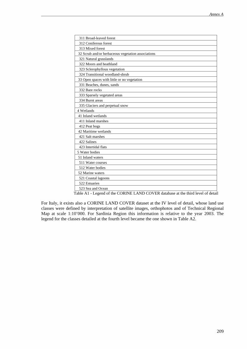
Annex A
209
311 Broad-leaved forest 312 Coniferous forest 313 Mixed forest 32 Scrub and/or herbaceous vegetation associations 321 Natural grasslands 322 Moors and heathland 323 Sclerophyllous vegetation 324 Transitional woodland-shrub 33 Open spaces with little or no vegetation 331 Beaches, dunes, sands 332 Bare rocks 333 Sparsely vegetated areas 334 Burnt areas 335 Glaciers and perpetual snow 4 Wetlands 41 Inland wetlands 411 Inland marshes 412 Peat bogs 42 Maritime wetlands 421 Salt marshes 422 Salines 423 Intertidal flats 5 Water bodies 51 Inland waters 511 Water courses 512 Water bodies 52 Marine waters 521 Coastal lagoons 522 Estuaries 523 Sea and Ocean
Table A1 - Legend of the CORINE LAND COVER database at the third level of detail
For Italy, it exists also a CORINE LAND COVER dataset at the IV level of detail, whose land use classes were defined by interpretation of satellite images, orthophotos and of Technical Regional Map at scale 1:10’000. For Sardinia Region this information is relative to the year 2003. The legend for the classes detailed at the fourth level became the one shown in Table A2.

Annex A
210
Table A2 - Legend of the CORINE LAND COVER database at the fourth level of detail All these layers are in vector polygon format. 2) Pedologic Map of Sardinia at scale 1:50’000 This map is a cartographic representation (vector polygon), at scale 1:50’000, of a set of pedologic parameters. The territory is divided into landscape units with homogeneous pedologic characteristics. In the following we list the parameters contained in the map and their codifying. Soil depth(cm):
Class Depth (cm) 1 >75 cm deep soils 2 30-75 cm moderately deep soils 3 15-30 cm thin soils 4 <15 cm very thin soils
Table A3 - Codifying of soil depth classes

Annex A
211
Rockiness (%) The superficial rockiness is the percent of rock outcrop according to FAO guidelines (FAO, 1990):
Class Rockiness (%) N None 0 % V Very Few 0 – 2 % F Few 2 – 5 % C Common 5 – 15 % M Many 15 – 40 % A Abundant 40 – 80 % D Dominant ≥ 80 %
Table A4 – Codifying of soil rockiness classes Stoniness (%) The superficial stoniness is the percent of coarse fragments (diameter > 2 mm) on the soil surface, described according to FAO guidelines (FAO, 1990):
Class Stoniness (%) N 0 % None V 0 – 2 % Very Few F 2 – 5 % Few C 5 – 15 % Common M 15 – 40 % Many A 40 – 80 % Abundant D ≥ 80 % Dominant
Table A5 – Codifying of soil stoniness classes Texture The soil texture is described according to the clay, silt, sand content.
Class Texture description 0 None 1 Coarse 18% ≤ clay and >65% sand 2 Medium 18% ≤ clay < 35% and ≥ 15% sand, or 18% ≤ clay and 15% ≤ sand <65% 3 Medium fine <35% clay and <15% sand 4 Fine 35% ≤ clay < 60% 5 Very fine ≤ 60% clay 6 Not applicable
Table A6 – Codifying of soil texture classes Drainage The soil profile drainage is described according to FAO guidelines (FAO, 1990):
Class Drainage description E Excessively rapid S Moderately rapid W Good M Moderate I Imperfect P Slow V Very Slow
Table A7 – Codifying of soil drainage classes

Annex A
212
Permeability Class Permeability
E Very slow < 0,1 cm/h S slow 0,1 – 0,5 cm/h D Moderately slow 0,5 – 2,0 cm/h M Moderate 2,0 – 6,0 cm/h R Rapid 6,0 – 12,5 cm/h Y Very rapid 12,5 – 25,0 cm/h X Extremely rapid ≥ 25 cm/h
Table A8 – Codifying of soil permeability classes AWC Topsoil Available Water Capacity
Class AWC description <100 mm/m Low
100-140 mm/m Medium 140-190 mm/m High
>190 mm/m Very high Table A9 – Codifying of soil AWC classes Soil fertility (soil organic matter content)
Class Fertility <1 Low 1-2 Medium 2-6 High >6 Very high
Table A10 – Codifying of soil fertility classes Density This is a continuous value whose unit of measure is g/cm3
Salinity
Class (mmhos/cm) Salinity description <4 Very low 6-8 Medium >12 Very high
Table A11 – Codifying of soil salinity classes 3) Map sheets The Map Sheets are cadastral maps at scale 1:2’000 grouped by municipality (i.e. each municipality comprehends one or more Map Sheets without sharing them with other municipalities). The format is vector polygons. 4) AGEA crop data 1995-2004 This dataset contains data about crops by AGEA (Agency for the Grants in Agriculture) relative to the years 1995 and 2004 respectively, spatialized over the Map Sheets at scale 1:2’000. To each Map Sheet it is associated the type and the extension (in hectares) of the cultural type. 5) AGEA zootechnical data 2004 This dataset contains information about the use of the land and the supplementary helps to zootechny in Sardinia, with a Map Sheet detail. Then there are AGEA data about the zootechnical consistence of bovine and ovine of Sardinia for the years 1995, 2003 and 2004, having a municipality detail. The format is vector polygons.

Annex A
213
6) Forest Map 1:100’000 This dataset (vector polygons) contains a classification of the regional territory in classes of forest cover. 7) Geolithology/Permeability Map 1:100’000 This is a cartographic representation (vector polygons) of geolithologic classes of Sardinia according to their permeability. 8) Geologic Map These are cartographic representation (both vector polygons at 1:200’000 and raster layers of sheets at scale 1:100’000) of geologic formations of Sardinia. 9) Digital Elevation Model It is a spatialized representation of terrain elevation. Each cell supplies a value of the elevation above the sea level. This dataset consists in a mosaic of IGM (Italian Military Geographic Institute) sections (http://www.igmi.org) at scale 1:25’000 for the whole territory of Sardinia. This datum was derived first scanning the IGM topographic map at scale 1:25’000, digitizing the contours lines and elevation points, then interpolating, georeferencing and mosaicing them until obtain a raster layer at 25 meters of resolution. 10) Railway maps This dataset contains the vector railway lines of Sardinia, obtained through the digitizing of railway network (using ortophotos and Regional Technical Map at scale 1:10’000). 11) GroundWater Resources This dataset (vector polygons) contains more informatic layers relative to hydrogeological characteristics of groundwater. Particularly useful was the theme describing the aquifer hydraulic properties. The scale is 1:500’000. 12) Hydrographic map This dataset (polyline and polygon dataset) identify the water bodies of the region (lakes, rivers, streams). It was derived digitizing the stream network using ortophotos and Regional Technical Map at scale 1:10’000. 13) Organic Carbon in Topsoil This datum is a raster digital data (obtained from http://eusoils.jrc.it/ESDB_Archive/octop/octop_data.html) and it is a representation at 1 km of resolution of the Topsoil Carbon content in percent. 14) Ortophotos This is a mosaic of digital ortophoto (black and white, referred to the year 1998) of Sardinia. Pixel resolution is 1 meter.
15) Wells The Agency for the Environment Protection and the Technical Services (APAT) computerized, in the context of the National Law 464/84, the information relative to wells. The Point dataset contains the following characteristics:
- geographic location (latitude-longitude); - depth of the static level of the wells; - elevation of the well a.s.l.; - piezometric elevation of the water table; - presence/absence of the groundwater and number of aquifer met; - maximum and mean discharge;

Annex A
214
- well depth; - top and bottom of the aquifer layer; - stratigraphy.
16) Meteorological data There are 17 meteorological stations whose data are managed by National Oceanic & Atmospheric Administration (NOAA): ASINARA ISLAND, GUARDIAVECCHIA, ALGHERO, CAPOCACCIA, MACOMER, OLBIA/COSTA SMERALDA, FONNI, CAPOFRASCA, PERDASDEFOGU, CAPO S. LORENZO, MOUNT SERPEDDI, DECIMOMANNU, CARLOFORTE, ISOLA DI CARLOFORTE, CAPO BELLAVISTA, CAGLIARI/ELMAS, LAMEZIA TERME, CAPO CARBONARA. These climatic data have daily time step and are referred to period from 1994 to 2005 and they regard in particular: mean temperature (°K), dew point temperature (°K), sea level pressure (Pa), wind speed (m/s), maximum wind speed (m/s), gust (m/s) maximum temperature (°K), minimum temperature (°K), total precipitation amount (mm), total snow fall amount (mm).
Moreover there are 6 meteorological stations whose data are managed by the Central Office of Agricultural Ecology (UCEA): ALGHERO, OLBIA, COSTA SMERALDA, CHILIVANI, CAPO BELLAVISTA, CAGLIARI ELMAS, SANTA LUCIA. The climatic parameters acquired by these stations have a daily time step and are referred to years comprised between 1994 and 2005, the list of variables can be found at http://www.politicheagricole.it/ucea/forniture/index3.htm Starting from these point data, they were derived spatializations for the years from 1991 to 1995 and from 2001 to 2005. the interpolations were carried out by the (a) Laboratorio di Simulazioni Numeriche del Clima e degli Ecosistemi Marini (University of Bologna, Italy) specifically for the project.
The spatialization was made at 1 km of resolution for the following variables: mean temperature (°K), dew point temperature (°K), precipitation (mm/day), daily maximum temperature (°K), daily minimum temperature (°K), mean wind speed (m/s), maximum wind speed (m/s) using the krigging procedure. For that concerning the solar radiation (W/m2), this parameter was acquired from MARS-STAT database (JRC, Ispra, Italy). The MARS-STAT Data Base contains meteo interpolated data from 1975, covering the EU member states, the central European eastern countries, the new Independent states and the Mediterranean countries. The daily meteorological data are interpolated into a 50x50 km grid. Further, they were used some spatialization of daily averages of meteo data, considering following periods of ten years: 1961-1970; 1971-1980; 1981-1990. These data were originally acquired by the PRUDENCE project web site. All this data were supplied as NetCDF format files available on the website of the Prudence project (http://prudence.dmi.dk/). The data were imported in raster format. The spatialized data (at 1 km of resolution by (a)) are: 2-m air mean daily temperature (°K), precipitation (mm/day), soil moisture (mm), 2-m maximum daily temperature (°K), 2-m minimum daily temperature (°K), mean daily wind speed (m/s), maximum daily wind speed (m/s), Incident Short Wave radiation (W/m2), Net Long Wave radiation (W/m2), Incident Short Wave radiation (W/m2). Then they were acquired directly from the regional services (Agro-meterological regional service) the data about 417 meteorological station of the region only for the precipitation parameter, whose values were supplied in a table format on a monthly basis, for the period from 1982 to 2003. 17) Road maps This dataset contains the vector road lines of Sardinia, obtained through the digitizing of road network (using orthophotos and Regional Technical Map at scale 1:10’000).

Annex A
215
18) Phenologic calendar This dataset stores information relative to sowing periods, bloom and harvesting of cultivated types. 19) Population census (1991-2001) This dataset contains results of the ISTAT (Italian National Institute of Statistics) censuses for the years 1991 and 2001 about socio-demographic-economic data at municipality detail. 20) Employment census (1992-2003) The data about employment (ISTAT) allowed to analyze the trend of work of the whole labour force. The detail of this datum is regional. 21) European soil database Another data source about soil characteristics for this study was the European Soil Database (ESDB), which originates from national soil surveys, following harmonization to provide a seamless spatial and thematic cover of European soil properties (King et al., 1994). The ESDB consists of two main databases, the Soil Geographic Database (SGDB) and the Pedo-Transfer Rules Database (PTRDB). Both databases were used to produce an European Raster Database, which contains a selected number of thematic soil properties as spatial data layers in raster format. This product is now available under request as raster layer at 1 km of resolution. 22) MODIS products FPAR/LAI (MOD15A2 product) The MODerate-resolution Imaging Spectroradiometer (MODIS) Leaf Area Index (LAI) and Fraction of Photosynthetically Active Radiation (FPAR) products are 1km global data products updated once each 8-day period throughout each calendar year. LAI defines an important structural property of a plant canopy as the one sided leaf area per unit ground area. FPAR measures the proportion of available radiation in the photosynthetically active wavelengths (400 to 700 nm) that a canopy absorbs. LAI and FPAR are related to functional process rates of energy and mass exchange.
MOD15A2 Image Characteristics ~ 10° x 10° lat/long Image dimensions 1200x1200 rows/columns Spatial Resolution 1000 meters Projection Sinusoidal Data format HDF-EOS Bands 4 Temporal Resolution 8 days
Table A12 – Characteristics of MOD15A2 image products NDVI (MOD13Q1 and MOD13A2 product) The MODIS Normalized Difference Vegetation Index (NDVI) products are contained into two datasets: the MOD13Q1 at 250 meters of resolution and the MOD13A2 at 1000 meters of resolution. Each scene of the product has following characteristics.
MOD13Q1 MOD13A2 Image Characteristics ~ 10° x 10° lat/long ~ 10° x 10° lat/long Image dimensions 4300x4100 rows/columns 1200x1200 rows/columns Spatial Resolution 250 meters 1000 meters Projection Sinusoidal Sinusoidal Data format HDF-EOS HDF-EOS Bands 11 11 Temporal Resolution 16 days 16 days
Table A13 – Characteristics of MOD13A2 and MOD13Q1 image products

Annex A
216
PRE-ELABORATION OF MODIS DATA The tool MODIS Reprojection Tool (supplied by Land Processes Distributed Active Archive Centre (LP-DAAC) - http://edcdaac.usgs.gov/landdaac/tools/modis/index.asp) was used to project and mosaic the images into the UTM Reference System - WGS84 zone 32N. Not only the images with associated the parameters (LAI, FPAR or NDVI) were processed, but also their relative images of quality check, showing the quality (reliability) of each pixel value. First we mosaiced the two images containing each one about half of the Sardinia territory and then we clipped the total images according to the following geographic limits:
North 41.35° East 10° South 38.7° West 8°
Table A14 – Characteristics of MOD13A2 and MOD13Q1 image products The process is resumed in the Figure A1.
Figure A1 – Example of original raster images (left) and after mosaicing and projection (right)
23) ASTER products They were acquired a set of remote sensed data from ASTER (Advanced Spaceborne Thermal Emission and Reflection Radiometer http://asterweb.jpl.nasa.gov/index.asp) sensor on TERRA satellite. The sensor is composed by three separated instruments differing for they spectral and radiometric characteristics: VNIR: Visible and Near InfraRed SWIR: ShortWave InfraRed TIR: Thermal InfraRed

Annex A
217
VNIR is the most appropriate instrument for our purposes because it has a resolution of 15 m, an image dimension of 3600 sq. km, and it register the signal on three bands comprised between 0.52 and 0.86 µm (Table A15).
Figure A15 – Characteristics of the VNIR System They were acquired 4 images, each one representative of one season, of the ASTER On-Demand L2 Surface Reflectance VNIR product supplying the reflectance values, this for the test area (see Chapter 10). In some case, according to the orbit position of the satellite, it was necessary to acquire two images and mosaic them. 24) AVHRR products Normalized Difference Vegetation Index (NDVI) composites are produced from multiple AVHRR (Advanced Very High Resolution Radiometer) daily observations that have been composed together to create a nearly cloud-free image showing maximum greenness. An NDVI ratio is produced from bands one and two of the AVHRR composite to produce a derived NDVI band composite, at 7 days of resolution.
Image characteristics AVHRR Spatial Resolution 1000 meters Projection Lambert Azimuthal Equal-Area Data format HDF-EOS Bands 1 Temporal Resolution 7 days
Figure A16 – Characteristics of the AVHRR products
VNIR characteristics Spatial resolution 15 meters Image Dimension 60 km x 60 km
Band 1 0.52 µm - 0.60 µm Band 2 0.63 µm- 0.69 µm Spectral ranges Band 3 0.78 µm - 0.86 µm

Annex B
218
ANNEX B Gap filling procedure for the LAI, FPAR and NDVI MODIS images In the following we will refer to PARAM (it stands for PARAMeter) to indicate LAI, NDVI and FPAR parameters. Further, we have to specify that, when in the following we will refer to an 8-days synthesis, it will regard LAI and FPAR images, for the NDVI images we have to assume a 16-days synthesis. The developed GAP FILLING procedure (whose flow chart is reported in Figure B1 for the LAI parameter) had the aim of eliminating from the original image the pixels not satisfying a given qualitative level selected using a look up table giving, for each value of the quality check image, the suggestion of accepting it or not. First we created a mask of pixels to be substituted in the PARAM image for the considered date (date t), referring to the quality check image for the same day. The we superimposed this mask to the images of the previous and next date (date t-1 and date t+1), already masked with their respective quality checks. In this way we found the values of the valid pixels in these two images, occupying the position to substitute to the date t. The mean of these two values of the previous and successive date is assigned to the correspondent pixel in the treated images of date t . At this point we create a further mask of pixels “invalid” after the first phase and the cycle is repeated with the images of the dates t-2 and t+2 and dates t-3 e t+3. In the case, during these steps, it will be not possible to obtain a valid values, as there are invalid values for the same pixel in all the images, to this pixel it will be assigned a no data value.
Figure B1 – Flow chart of the Gap-Filling procedure in the case of LAI parameter
Example: let us imagine to do the gap-filling of the image dated January 25th, 2003 (referred to the 8-days synthesis January 25th-February 1st), the first correction will be made with the images relative to the 8-days synthesis immediately precedent (17th January) and successive (2nd February), while the two successive corrections will consider respectively the dates of 9th January and of 10th February, and of 1st January and 27th December.

Annex C
219
ANNEX C Downscaling methodology for the MODIS products for the year 2003 The objective of this methodology was to re-scale the remote sensed product of LAI (Leaf Area Index) and FPAR (Fraction of Photosynthetically Active Radiation), in the following simply PARAM, from the resolution of 1000 m to 50 m. In particular the downscaling procedure was divided into two steps: the former from 1000 m to 250 m (regarding the LAI and FPAR), the latter from 250 m to 50 m (regarding LAI, FPAR and NDVI). Downscaling from 1000m to 250m After the gap-filling (Annex B) we obtained corrected images at 1000 m of resolution. To downscale these images to 250 meters of resolution we decided to use the relationship existing between the PARAM (FPAR or LAI) and the NDVI: in this case the 16-days synthesis of NDVI was divided into two syntheses of 8 days in order to match with the 8-days syntheses of PARAM. In the following (Figure C1) we reported an example of regression lines examined between LAI and NDVI images for the same date, on a land use basis (third level of the Corine Land Cover database). We extracted a relationship for each date.
Figure C1 – Example of regression line between the PARAM (in this case LAI) and NDVI (MODIS) at 1 km of resolution, useful to find the relationship used in the downscaling of datum from 1000 m to 250 m. While the PARAM is available only at resolution of 1000 m, the NDVI is both at 1000 m and at 250 m of resolution (13Q1 product). For each date, the found relationship was then re-applied using the NDVI at 250 m of resolution and deriving a “synthetic” PARAM value at 250 meters of resolution.

Annex C
220
Downscaling from 250 m to 50m To pass to 50 m of resolution for PARAM we used a methodology considering the land use to which the parameter is associated. For the year 2003 we created an image at 250 meters of resolution of the land use, reclassified according to the Table C1:
Land Use 1 Urban 2 Agricultural Surfaces 3 Broadleaves forest and mixed with prevalent broadleaf 4 Needleleaves forest and mixed with prevalent needleleaf 5 Areas with shrub vegetation or sparse vegetation 6 Wet areas and water bodies
Table C1 – Reclassification of the macro-classes applied to the Corine Land Cover 2003 Considering this Map we made a zonal statistics of the values correspondent to the same land use class, obtaining a value of PARAM for each typology, and we associated this mean value to the same map of land use, but resampled to 50 m (Figure C2), this layer is referred as Raster1. Figure C2 – Sketch of result of the zonal statistics over the PARAM layer and the successive resampling to 50 meters of resolution. At this point we averaged the PARAM values of the 25 pixels at 50 meters of resolution contained into a pixel at 250 meters of resolution (that can also be a mixed pixel), obtaining a mean value at 250 meters of resolution, then we re-sampled this result to 50 meter of resolution, obtaining the layer Raster2. Dividing the Raster1 by the Raster2, we obtained a raster of weights that is able to consider also the frequency of pixel at 50 meters of resolution for each class present into a pixel of 250 meters of resolution. Multiplying this weight for the remote sensed datum at 250 meters previously downscaled, we obtain a layer at 50 m relative to the PARAM. In some case we can obtain from this procedure saturated values (greater than 100, the maximum value acceptable in the image), these values are set to 100. Finally, all the values were multiplied by 0.1 (fort he LAI) and 0.01 (for the FPAR), in order to re-scale the PARAM (LAI or FPAR) to the right range of values. This procedure was used also to downscale the NDVI MODIS from 250 to 50 meters of resolution.

Annex D
221
ANNEX D Downscaling methodology for the MODIS products for the 1995 images The objective of this methodology was to re-scale the synthetically remote sensed products (see Par. 3.4.6 Chapter 3, Par. 5.3 Chapter 5 and Par. 7.5.6 chapter 7) of NDVI (Normalized Difference Vegetation Index), FPAR (Fraction of Photosynthetically Active Radiation) and LAI (Leaf Area Index), in the following simply PARAM, from the resolution of 1000 m to 50 m starting from the real or synthetic image relative to the early nineties. Downscaling from 1000m to 50m To pass to 250 m of resolution of the PARAM datum we used a methodology considering the land use to which the parameter is associated. For the year 1990 we created an image at 1000 meters of resolution of the land use, reclassified according to the Table D1:
Land Use 1 Urban 2 Agricultural Surfaces 3 Broadleaves forest and mixed with prevalent broadleaf 4 Needleleaves forest and mixed with prevalent Needleleaf 5 Areas with shrub vegetation or sparse vegetation 6 Wet areas and water bodies
Table D1 – Reclassification of the macro-classes applied to the Corine Land Cover2003 Considering this Map we made a zonal statistics of the values correspondent to the same land use class, obtaining a value of PARAM for each typology, and we associated this mean value to the same map of land use, but resampled to 250 m (Figure D2), this layer is referred as Raster1.
Figure D2 – Result of the zonal statistics over the PARAM layer and the successive resampling to 250 meters of resolution. At this point we averaged the values of the 20 pixels at 250 meters of resolution contained into a pixel at 1000 meters of resolution (that can also be a mixed pixel), obtaining a mean value at 1000 meters of resolution, then we re-sampled again the layer to 250 meter of resolution, obtaining the layer Raster2.

Annex D
222
Dividing the Raster1 by the Raster2, we obtained a raster of weights that are able consider also the frequency of pixel at 250 meters of resolution for each class present into a pixel of 1000 meters of resolution. Multiplying this weight for the remote sensed datum at 1000 meters, we obtain a layer at 250 m relative to the PARAM. In some case there we obtained from this procedure saturated values (greater than 100 for FPAR and LAI, and greater than 10000 for NDVI, the maximum values acceptable), that we reset to 100 or 10000, respectively. Finally, all the values were multiplied by 0.1 (fort he LAI), 0.01 (for the FPAR) and by 0.0001 for NDVI, in order to re-scale the PARAM to the right range of values. Successively, the downscaling to 50 meters of resolution was a simple resampling, because of the lack of detailed data to reach this resolution by means of more reliable procedures.
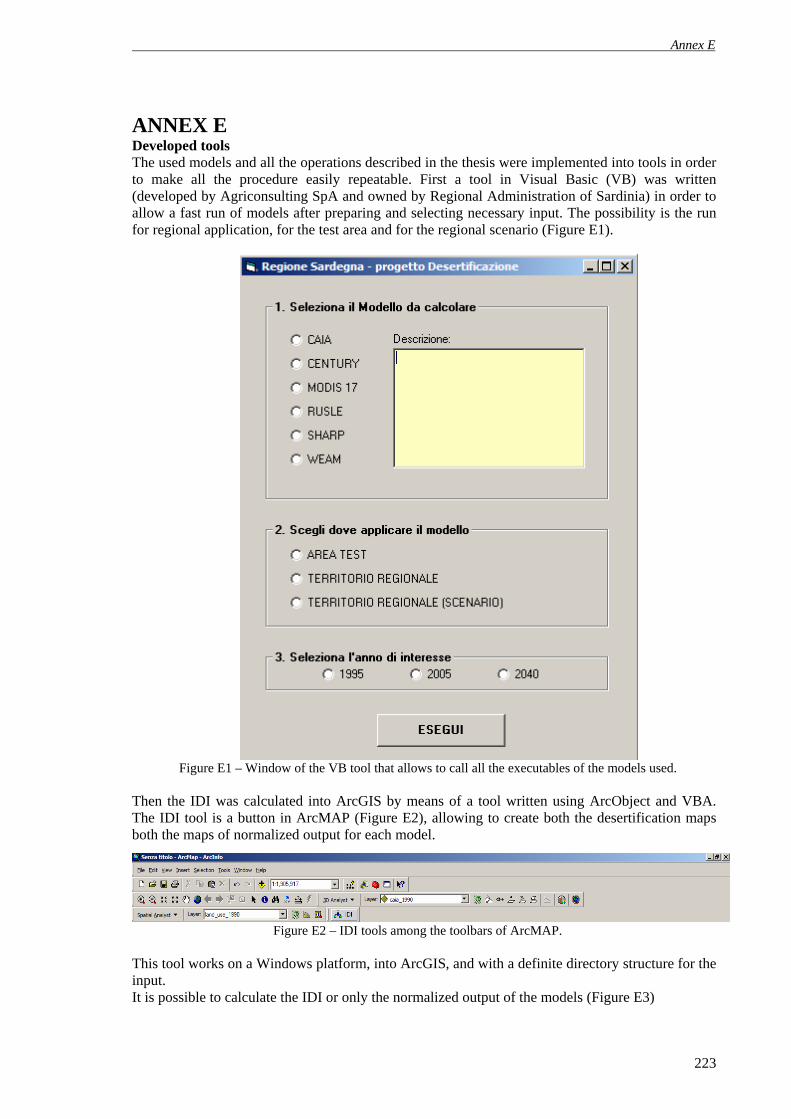
Annex E
223
ANNEX E Developed tools The used models and all the operations described in the thesis were implemented into tools in order to make all the procedure easily repeatable. First a tool in Visual Basic (VB) was written (developed by Agriconsulting SpA and owned by Regional Administration of Sardinia) in order to allow a fast run of models after preparing and selecting necessary input. The possibility is the run for regional application, for the test area and for the regional scenario (Figure E1).
Figure E1 – Window of the VB tool that allows to call all the executables of the models used. Then the IDI was calculated into ArcGIS by means of a tool written using ArcObject and VBA. The IDI tool is a button in ArcMAP (Figure E2), allowing to create both the desertification maps both the maps of normalized output for each model.
Figure E2 – IDI tools among the toolbars of ArcMAP. This tool works on a Windows platform, into ArcGIS, and with a definite directory structure for the input. It is possible to calculate the IDI or only the normalized output of the models (Figure E3)

Annex E
224
Figure E3 – Window of the IDI tool that allows to choose the area for the application, to select the parameters (directories of input etc.) and to choose if showing as result only the IDI or also the normalized output of the model Then the tool permits to choose the weights to give to the models (Figure E4)
Figure E4 – Window of the IDI tool that allows to choose the weights to give to the indices and to the variation of them and to select the name of output map. This tool was also developed as tool of Arctoolbox into ArcGIS and as AML (Arc Macro Language) executable.

Università degli Studi della Tuscia Dipartimento di Scienze dell’Ambiente Forestale e delle sue Risorse (DISAFRI) Via S. Camillo de Lellis, snc 01100 Viterbo Corso di Dottorato di Ricerca in Ecologia Forestale Coordinatore: Prof. Paolo De Angelis Tesi di Dottorato di Ricerca in Ecologia Forestale (XX ciclo) di: Monia Santini Marzo 2008

Ringraziamenti
I miei ringraziamenti vanno prima di tutto al Prof. Riccardo Valentini che mi ha permesso di gestire ed affrontare con molta indipendenza il tema della ricerca, dandomi piena fiducia anche nell’avvicinarmi ad argomenti per me completamente nuovi.
Questo lavoro, certo, non sarebbe stato possibile senza il gruppo migliore che mi potesse capitare per svolgerlo, sia dal punto di vista professionale che umano; per questo ringrazio la Dr.ssa Paola Molinari, il Dott. Gabriele Caccamo, il Dott. Alberto Laurenti e il Dott. Sergio Noce, con i quali ho lavorato in un clima fantastico anche nei momenti più difficili.
Il mio grazie va anche al Dr. Claudio Belli per il supporto dato da Terrasystem, a tutto il gruppo degli esperti dell’Università di Sassari, senza i quali una parte del lavoro non sarebbe stata possibile: il Dott. Daniele Pittalis, la Dott.ssa Ileana Iocola, il Dott. Domenico Soru, e a tutti coloro che hanno revisionato e valutato il lavoro passo passo, in quanto responsabili diretti, permettendomi di migliorarlo: l’Ing. Nicoletta Sannìo, la Dr.ssa Francesca Cotza e la Dott.ssa Silvia Serra della Regione Sardegna.
Ringrazio ovviamente il Dr. Paolo Ciccioli per i suoi costanti e sempre utili consigli ed il Prof. Paolo de Angelis per la serietà con cui ha sempre coordinato noi dottorandi.
Ma al di là del lavoro della tesi, questo periodo di dottorato è stato allietato dalla presenza e dal supporto del gruppo del Laboratorio di Ecologia Forestale in cui ho lavorato, in particolare Cristina, Manuela, Massimo, Nicola e Renato, persone straordinarie con le quali ho condiviso momenti piacevolissimi.
E per questi ultimi due anni devo molto del mio entusiasmo e della mia crescita ad un gruppo di ricerca speciale fatto di persone decisamente impagabili per avermi dato la possibilità di fare esperienze professionali ed umane uniche: il Prof. Salvatore Grimaldi, il Dr. Fernando Nardi, il Dr. Andrea Petroselli.
Infine, un pensiero a parte merita la mia famiglia, sulla quale ho sempre potuto contare e per la quale ogni parola sarebbe insufficiente a descrivere la mia gratitudine: Noemi, Francesco, Papà e Mamma.