A NEW DESIGN METHODOLOGY FOR MODULAR BROADBAND …

The Pennsylvania State University

The Graduate School

College of Engineering

A NEW DESIGN METHODOLOGY FOR MODULAR BROADBAND ARRAYS BASED ON FRACTAL TILINGS

A Thesis in

Electrical Engineering

by

Waroth Kuhirun

Submitted in Partial Fulfillment of the Requirements

for the Degree of

Doctor of Philisophy

August 2003

© 2003 by Waroth Kuhirun

We approve the thesis of Waroth Kuhirun. Date of Signature ____________________________ ___________________ Douglas H. Werner Associate Professor of Electrical Engineering Thesis Adviser Chair of Committee ___________________________ ___________________ Raj Mittra Professor of Electrical Engineering ____________________________ ____________________ James K. Breakall Professor of Electrical Engineering ____________________________ ____________________ Pingjuan L. Werner Associate Professor of Engineering ____________________________ _____________________ Brian Weiner Associate Professor of Physics ____________________________ _____________________ W. Kenneth Jenkins Professor of Electrical Engineering Head of the Department of Electrical Engineering

iii

Abstract

In this thesis, a new and innovative technique based on the theory of fractal tilings

is introduced for the design of modular broadband arrays. These arrays are unique in the

sense that they possess a fractal boundary contour that tiles the plane without gaps or

overlaps. The first of these new array configurations that will be considered is directly

related to the family of space-filling and self-avoiding fractals known as Peano-Gosper

curves. The elements of the fractal array are uniformly distributed along a Peano-Gosper

curve, which leads to a planar array configuration with parallelogram cells that is

bounded by a closed Koch curve. These unique properties are exploited in order to

develop a design methodology for deterministic arrays that have no grating lobes even

when the minimum spacing between elements is increased to at least one-wavelength.

This leads to a class of arrays that are relatively broadband when compared to more

conventional periodic planar arrays with square or rectangular cells and regular boundary

contours. This type of fractal array differs fundamentally from other types of fractal array

configurations that have been studied previously that have regular boundaries with

elements distributed in a fractal pattern on the interior of the array.

An efficient iterative procedure for calculating the radiation patterns of these

Peano-Gosper fractal arrays to arbitrary stage of growth P is also introduced in this

thesis. Moreover, we note that Peano-Gosper arrays are self-similar since they may be

formed in an iterative fashion such that the array at stage P is composed of seven

identical stage P-1 sub-arrays (i.e., they consist of arrays of arrays). This lends itself to a

convenient modular architecture whereby each of these sub-arrays could be individually

controlled. In other words, the unique arrangement of tiles forms sub-arrays that could be

iv

designed to support simultaneous multibeam and multifrequency operation. Finally,

several other examples of fractal tilings that lead to broadband array configurations will

be considered including terdragon and 6-terdragon arrays.

This thesis also introduces several new self-scalable arrays that can be generated

by repeated application of a ring subarray generator, including pentagonal, octagonal, and

honeycomb arrays. These arrays have the advantage that they can be recursively

generated, allowing development of rapid algorithms for calculating their radiation

patterns. They are also shown to possess relatively low sidelobe levels. Lastly, the

radiation characteristics of some basic three-dimensional volumetric fractal arrays

generated using concentric sphere subarrays will be briefly considered.

v

TABLE OF CONTENTS Page LIST OF TABLES............................................................................................... ix LIST OF FIGURES .............................................................................................. x ACKNOWLEDGEMENTS................................................................................ xx Chapter 1 Background............................................................................................... 1

1.1 Fractal Arrays using Circular and Concentric Ring Subarray Generator .................................................................... 4

1.1.1 Sierpinski Gasket Array Pattern.......................................... 8

1.1.2 Self-Scalable Hexagonal Array Pattern ............................. 14

1.2 Mathematical Tools for determining the Performance of Fractal Arrays ............................................................................... 25 1.2.1 Directivity .......................................................................... 25

1.2.2 Plot of Array Factor in Terms of n or Ψ .......................... 26

2 Fractal Arrays Using Ring Subarray Generators .................................... 30

2.1 Self-Scalable Pentagonal Arrays....................................................... 30

2.2 Self-Scalable Octagonal Arrays........................................................ 40

2.3 Honeycomb Fractal Arrays ............................................................... 50

vi

TABLE OF CONTENTS (continued)

Chapter Page

2.3.1 Results of Honeycomb Fractal Arrays............................... 51

2.4 Conclusion ........................................................................................ 53

3 Generalized Principle of Pattern Multiplication and Multiple-Generator Fractal Arrays ......................................................... 55 3.1 Conventional Principle of Pattern Multiplication ............................. 55

3.2 Generalized Principle of Pattern Multiplication ............................... 56

3.3 Fractal Arrays Generated by Multiple Generators............................ 59

4 Peano and Sierpinski Dragon Fractal Arrays.......................................... 62

4.1 Construction of the Peano Curve ...................................................... 62

4.2 Construction of the Peano Fractal Array .......................................... 66

4.3 The Construction of Sierpinski Dragon Array.................................. 79

4.4 Sierpinski Dragon Arrays ................................................................. 82

5 The Peano-Gosper Fractal Array ............................................................ 89

5.1 Construction of Peano-Gosper Curves.............................................. 90

5.2. Construction of the Peano-Gosper Fractal Array............................. 93

5.3. Results............................................................................................ 101

5.4. Conclusions.................................................................................... 113

6 Broadband Arrays Produced by Fractal Tilings.................................... 114

6.1 The Terdragon and the 6-Terdragon Arrays ................................... 114

6.1.1. Construction of the Terdragon Fractal Array ................................................................... 117

vii

TABLE OF CONTENTS (continued) Chapter Page

6.1.2. Construction of the 6-Terdragon Fractal Array ................................................................... 120

6.1.3. Radiation Characteristics of the Terdragon and 6-Terdragon Fractal Arrays .................... 122

6.1.4 Conclusions...................................................................... 139

7 Coordinate Transformation for 3-D Antenna Arrays and its Application to Beamforming............................................................ 140

8 3-D Fractal Arrays Using Concentric Sphere Array Generators ............................................................................................. 147 8.1 Introduction..................................................................................... 147

8.2 Synthesis of 3-D Fractal Arrays using Concentric Sphere Array Generators................................................................. 148

8.2.1 Menger Sponge (3-D Sierpinski Carpet) Array ............... 151

8.2.1.1 Results of Menger Sponge Arrays .................... 156

8.2.2 3-D Sierpinski Gasket Arrays .......................................... 159

8.2.2.1 Results of the Stage 3 3-D Sierpinski Gasket Array ..................................................... 164

8.3 Conclusions..................................................................................... 168

9 Conclusions and Future Work ............................................................. 169

9.1 Conclusions .................................................................................... 169

9.2 Future Work .................................................................................... 172

References......................................................................................................... 174

Appendix: A.1 Directivity of 2-D (Planar) Arrays containing N in-phase isotropic elements .................................................. 179

viii

TABLE OF CONTENTS (continued)

Chapter Page

A.2 Directivity of 3-D Antenna Arrays containing

N isotropic Elements ...................................................................... 182

A.3 Array Factor of 2-D (Planar) Arrays Expressed in terms of

Ψ or n ........................................................................................... 185

ix

LIST OF TABLES

Page 2.1 Comparison of maximum directivity for a stage 3 unmodified self-scalble octagonal array and a stage 3 modified self-scalable octagonal array..........................................................................................................50 4.1 The parameters xn and yn expressed in terms of dmin ................................................84

5.1 Expressions for ),( nn yx in terms of the array parameters α,mind ,andδ ..........................................................................................................100 5.2 The maximum directivity for several different Peano-Gosper fractal arrays...................................................................................109 5.3 Comparison of maximum directivity for a stage 3 Peano-Gosper array with 344 elements and a 19x19 square array with 361 elements...........................110 6.1 Expressions of xn and yn in terms of the parameters dmin, α and δ .........................120

6.2 Maximum directivity for several different terdragon fractal arrays .......................134

6.3 Maximum directivity for several different 6-terdragon fractal arrays ....................135

6.4 Comparison of maximum directivity of a stage 6 terdragon array of 308 elements with a 18x18 square array of 324 elements ......................................136 6.5 Comparison of maximum directivity of a stage 3 6-terdragon array of 79 elements with a 9x9 square array of 81 elements ..............................................136

x

LIST OF FIGURES

1.1 Geometry for an M-ring subarray generator where each ring has a total of N elements. The location of the mnth element is shown .......................5 1.2 Ring subarray generators ...................................................................................6 1.3 Sierpinski gasket ................................................................................................9 1.4 Various stages of growth for the Sierpinski gasket array .................................10 1.5 Plot of the Sierpinski gasket array factor for various stages of growth with kr = 3.........................................................................................................12 1.6 Plot of the Sierpinski Gasket array factor for various stages of growth with kr = 1.5......................................................................................................14 1.7 Self-scalable hexagonal antenna array..............................................................15 1.8 Figures representing the self-scalable hexagonal antenna array.......................16 1.9 The array factor pattern of self-scalable hexagonal array (Stage 1) .................19 1.10 The array factor pattern of self-scalable hexagonal array (Stage 2) .................20 1.11 The array factor pattern of self-scalable hexagonal array (Stage 3) .................22 1.12 The array factor pattern of self-scalable hexagonal array (Stage 4) .................23 1.13 The array factor pattern of self-scalable hexagonal array (Stage 5) .................25 1.14 Figure to show representation of array factor for 2-D (Planar) arrays in terms of nx and ny ..........................................................................................27 1.15 Figure to show representation of array factor for 3-D arrays in terms

of nx, ny and nz ...................................................................................................29 2.1 5-element ring subarray generator ....................................................................30 2.2 Geometry relating expansion ratio δ and dmin for a pentagon subarray generator............................................................................................31 2.3 Self-scalable pentagonal antenna array.............................................................33

xi

2.4 Array factor plot for self-scalable pentagonal array at stage 3 .........................34 2.5 Array factor of the self-scalable stage 3 pentagonal antenna array at stage 3 with minimum spacings of 0.5λ (dashed curve) and λ (solid curve) at °= 0ϕ ....................................................................................35 2.6 5-element subarray generator modified by inserting an element at the center......................................................................36 2.7 Self-scalable pentagonal array whose subarray generator is

modified by inserting one element at the center ..............................................37

2.8 Array factor plots for self-scalable pentagonal array at stage 3 modified by inserting an element at the center of the generator......................39

2.9 The array factor of the stage 3 modified self–scalable pentagonal

array for minimum element spacings 0.5λ (dashed curve) and λ (solid curve) at ϕ = 0° ............................................................................40

2.10 8-element ring subarray generator ...................................................................41 2.11 Geometry relating to expansion ratio δ and dmin

for an octagonal subarray generator.................................................................41 2.12 Self-scalable octagonal antenna array..............................................................43 2.13 Array factor plots for self-scalable octagonal array at stage 3.........................44 2.14 Array factor of self-scalable stage 3 octagonal antenna array with minimum spacing of 0.5λ (dashed curve) and λ (solid curve) at ϕ = 0° ..................................................................................45 2.15 Self-scalable octagonal array whose subarray generator is modified by inserting an element at the center ............................................47 2.16 Array factor plots for self-scalable octagonal array at stage 3 inserting an element at the center of the generator ..........................................48

2.17 Array factor of self–scalable octagonal array at stage 3 with minimum spacings of 0.5λ (dashed curve) and λ (solid curve) modified by inserting an element at ϕ = 0°.............................49 2.18 Stage 3 honeycomb fractal array......................................................................51

xii

2.19 Plot of normalized array factor of the stage 3 honey comb fractal array with dmin = λ ............................................................................................52 2.20 Plot of array factor of the stage 3 honeycomb array sliced at ϕ = 0° for dmin = 0.5λ (dashed curve) and dmin = λ (solid curve) ....................52 4.1(a) Initiator of the Peano curve..............................................................................62 4.1(b) Generator for the horizontal generating line....................................................63 4.1(c) Generator for the vertical generating line ........................................................64 4.2(a) Peano curve (at stage 1) ...................................................................................65 4.2(b) Peano curve (at stage 2) ..................................................................................66 4.3 Initiator element of the Peano curve array.......................................................67 4.4 Subarray generator of the Peano curve array...................................................67

4.5 Figure to illustrate fp,11(θ,φ) and fp,21(θ,φ) ........................................................69

4.6(a) Construction of the Peano fractal array (at step 1) ..........................................74 4.6(b) Construction of the Peano fractal array (at step 2) .........................................74

4.6(c) Construction of the Peano fractal array (at step 3) ..........................................75 4.6(d) Construction of the Stage 2 Peano fractal array (at step 4)..............................75 4.7(a) Peano fractal array (at stage 1).........................................................................76 4.7(b) Peano fractal array (at stage 2).........................................................................77 4.8 Plot of normalized array factor for a stage 3 Peano fractal array with minimum spacing dmin = λ with respect to nx and ny ...............................................78 4.9 Normalized array factor of the Peano curve array at °= 0ϕ , stage 3, dmin = 0.5λ (dashed curve) and dmin = λ (solid curve) ........................79 4.10(a) Initiator of Sierpinski dragon ...........................................................................80 4.10(b) Stage 1 Sierpinski dragon curve, generator is shown by solid curve, whereas the dashed line represents the initiator ...........................80

xiii

4.10(c) Construction of the Sierpinski dragon curve (stage 2).....................................80 4.11 Sierpinski dragon .............................................................................................81 4.12(a) The stage 3 Sierpinski dragon array.................................................................85 4.12(b) The stage 5 Sierpinski dragon array.................................................................85 4.13 Plot of the normalized Sierpinski dragon array factor at stage 5 with dmin = λ with respect to nx and ny...................................................................86 4.14 Plot of stage 3 Sierpinski dragon normalized array factor for ϕ = 0° with minimum spacings of dmin = λ (solid curve) and dmin = 0.5λ (dashed curve) ........................................................................87 4.15 Plot of stage 5 Sierpinski dragon normalized array factor for ϕ = 0° for minimum spacings of dmin = λ (solid curve) and dmin = 0.5λ (dashed curve) ...............................................................................88 5.1 The Peano-Gosper curve initiator ....................................................................90 5.2 The Peano-Gosper curve generator..................................................................91 5.3 The first three stages in the construction of a self-avoiding Peano-Gosper curve. The initiator is shown as the dashed line superimposed on the stage 1 generator. The generator (unscaled) is shown again in (b) as the dashed curve superimposed on the Stage 2 Peano-Gosper curve ..........................................92 5.4 Gosper islands and their corresponding Peano-Gosper curves for (a) stage 1, b) stage 2, and (c) stage 4 ........................................................93 5.5 Element locations and associated current distribution for Stages 1-3 Peano-Gosper fractal arrays with minimum spacing between elements and expansion factor denoted by mind and ,δ respectively. Note that the spacing mind between consecutive array elements along the Peano-Gosper curve is assumed to be the same for each stage .................................................................................94 5.6 Generating elements with n = 1 to n = 7 are located along the stage 1 Peano-Gosper curve.............................................................................95

xiv

5.7 Plots of the normalized stage 3 Peano-Gosper fractal array factor versus θ for ϕ = 0°. The dashed curve represents the case where 2/min λ=d and the solid curve represents the case where λ=mind .................................................................................101 5.8 Plots of the normalized stage 3 Peano-Gosper fractal array factor versus θ for ϕ = 90°. The dashed curve represents the case where 2/min λ=d and the solid curve represents the case where λ=mind ..............................................................................................102 5.9 Plot of the normalized stage 3 Peano-Gosper fractal array factor versus ϕ for θ = 90° and dmin = λ .......................................................102 5.10 Plot of the normalized stage 3 Peano-Gosper curve fractal array factor as a function of nx = sin θ cosϕ and ny = sin θ sin ϕ with dmin = λ .......................................................................103 5.11 Plot to show maximum allowable angle (θmax) versus minimum spacing between adjacent elements dmin in λ for the stage 3 Peano-Gosper fractal array ............................................................................104 5.12 Plot of the normalized stage 3 Peano-Gosper fractal array factor versus θ for ϕ = 26° and dmin = λ .................................................................105 5.13 Plots of the normalized array factor versus θ with ϕ = 0° for a uniformly excited 19x19 periodic square array. The dashed curve represents the case where 2/min λ=d and the solid curve represents the case where λ=mind ................................106 5.14 Plots of the normalized array factor versus θ with ϕ = 0° and λ2min =d for a stage 3 Peano-Gosper fractal array (solid curve) and a uniformly excited 19x19 square array (dashed curve).......................................................................................106 5.15 Plots of the normalized array factor versus θ for ϕ = 0° with mainbeam steered to θo = 45° and ϕo = 0°. The solid curve represents the radiation pattern of a stage 3 Peano-Gosper fractal array with 2/min λ=d and the dashed curve represents the radiation pattern of a uniformly excited 19x19 square array with 2/min λ=d ............................................................................................111

xv

5.16 Modular architecture of the Peano-Gosper array based on the tiling of Gosper islands. A stage 2 and stage 4 Peano-Gosper array are shown divided up into seven stage 1 and stage 3 Peano-Gosper sub-arrays respectively...........................................................112 6.1(a) Initiator for a terdragon curve ........................................................................114 6.1(b) Construction of a stage 1 terdragon curve. The solid curve denotes the generator whereas the dashed curve denotes the initiator...........114

6.1(c) Construction of a stage 2 terdragon curve. The solid curve denotes the generator for the terdragon curve or the stage 2 terdragon curve whereas the dashed curve denotes the stage 1 terdragon curve ..............................................................................................115

6.2 Stage 6 terdragon curve .................................................................................115 6.3 The first stage in the construction of a 6-terdragon. The initiator is shown as the dashed line superimposed on the stage 1 generator.............116 6.4 Stage 3 6-terdragon........................................................................................116 6.5 Element locations and associated current distribution for the stage 1, stage 3, and stage 6 terdragon fractal arrays with the minimum spacing between elements and expansion factor denoted by dmin and δ, respectively. dmin is assumed to be the same for each stage ........................................................................................117 6.6 Element locations and associated current distribution for the stage 1, stage 2 and stage 3 6-terdragon fractal arrays with the minimum spacing between elements and expansion factor denoted by dmin and δ respectively. dmin is assumed to be the same for each stage ...............................................121 6.7 Plot of the normalized array factor for the stage 6 terdragon fractal array factor with minimum spacing dmin = λ in terms of nx and ny ..........................................................................................................................................122 6.8 Plot of the normalized array factor of the stage 6 terdragon fractal array with minimum spacing dmin = λ in terms of nx and ny .........................................................................................................................................................123 6.9 Plot of the normalized array factor for the stage 3 6-terdragon fractal array factor with minimum spacing dmin = λ in terms of nx and ny .........................................................................................................................................................124

xvi

6.10 Plot of the normalized array factor of the stage 3 6-terdragon fractal array with minimum spacing dmin (0.5λ ≤ dmin ≤ λ) ............................125 6.11 Plot of the normalized stage 6 terdragon fractal array factor versus θ for ϕ = 0° for dmin = λ/2 (dashed curve) and dmin = λ (solid curve) ...............................................................................126 6.12 Plot of the normalized stage 6 terdragon fractal array factor versus θ for ϕ = 90° for dmin = λ/2 (dashed curve) and dmin = λ (solid curve) ...............................................................................126

6.13 Plot of the normalized stage 3 6-terdragon fractal array factor versus θ for ϕ = 0° for dmin = λ/2 (dashed curve) and dmin = λ (solid curve) ...............................................................................127 6.14 Plot of the normalized stage 3 6-terdragon fractal array factor versus θ for ϕ = 90° for dmin = λ/2 (dashed curve) and dmin = λ (solid curve) ...............................................................................127 6.15 Plot of the normalized stage 6 terdragon fractal array factor versus ϕ for θ = 90° and dmin = λ ................................................................128 6.16 Plot of normalized stage 3 6-terdragon fractal array factor versus ϕ for θ = 90° and dmin = λ ................................................................129 6.17 Plot of the normalized stage 6 terdragon fractal array factor versus θ for ϕ = 97° .......................................................................................129 6.18 Plots of the normalized stage 3 6-Terdragon fractal array factor versus θ for ϕ = 11° ............................................................................130 6.19 Plot of the normalized array factor versus θ at ϕ = 0° for a uniformly excited 18x18 periodic square array for dmin = λ/2 (dashed curve) and dmin = λ (solid curve)....................................131

6.20 Plot of the normalized array factor versus θ with ϕ = 0° for a uniformly excited 9x9 periodic square array for dmin = λ/2 (dashed curve) and dmin = λ (solid curve)....................................131

xvii

6.21 Plot of the normalized array factor versus θ with ϕ = 0° with dmin = 2λ for the stage 6 terdragon fractal array (solid curve) and a uniformly excited 18x18 square array (dashed curve).......................................................................................133 6.22 Plot of the normalized array factor versus θ for ϕ = 0° and dmin = 2λ for stage 3 6-terdragon fractal array (solid curve) and a uniformly excited 18x18 square array (dashed curve) .........................133 6.23 Plots of the normalized array factor versus θ for ϕ = 0° and dmin = λ/2 with mainbeam steered to θo = 45° and ϕo = 0°. The solid curve represents the radiation pattern of a stage 6 terdragon fractal array, and the dashed curve represents the radiation pattern of a uniformly excited 18x18 square array.........................138 6.24 Plots of the normalized array factor versus θ for ϕ = 0° and dmin = λ/2 with mainbeam steered to θo = 45° and ϕo = 0°. The solid curve represents the radiation pattern of a stage 3 6-terdragon fractal array, and the dashed curve represents the radiation pattern of a uniformly excited 9x9 square array .......................138 7.1 Rectangular coordinates (xn,yn,zn) and cylindrical coordinates ( )nnn z,,ϕρ and projection plane in the direction of ϕ = ϕo and θ = θo ..............141 7.2 Projection plane and the cylindrical coordinate system.................................144 8.1 Fractal spherical array initiator (stage 0) .......................................................149 8.2 Fractal spherical array (stage 1).....................................................................150 8.3 Menger sponge subarray generator, where each individual element is represented by a cube ...................................................................152 8.4 Subarray generator of Menger sponge arrays where each individual element is denoted by an “• ”. The minimum spacing between elements is dmin......................................................................................................153 8.5 Stage 2 Menger sponge (3-D Sierpinski carpet) array where an individual element is located at the center of each cube ................154 8.6 Top view of the stage 2 Menger sponge array in terms of minimum interelement spacing dmin.........................................................................................154

8.7 Front view of the stage 2 Menger sponge array, in terms of minimum interelement spacing dmin.........................................................................................155

xviii

8.8 Auxiliary view of the stage 2 Menger sponge array, in terms of interelement spacing dmin. The z′ -axis is oriented to the

direction of °= 45θ and °= 0ϕ . The scale is expressed in terms of dmin ......................................................................................................................................................155

8.9 Plot of the normalized array factor for the stage 2 Menger sponge array with minimum spacing of dmin = λ where mainbeam is steered to the direction of °== 0oθθ and °== 0oϕϕ .............................................156

8.10 Plot of the normalized array factor sliced at ϕ = 0º for the stage 2 Menger sponge array with minimum spacing of dmin = λ where mainbeam is steered to the direction of

°== 0oθθ and °== 0oϕϕ ...........................................................................157 8.11 Plot of the normalized array factor for the stage 2 Menger Sponge Array with minimum spacing of dmin = λ where mainbeam is steered to the direction of °== 45oθθ and °== 0oϕϕ . The horizontal and vertical axes denote xn and yn , respectively,

where 1222 =++ zyx nnn ..................................................................................158

8.12 Plot of the normalized array factor for the stage 2 Menger Sponge Array with minimum spacing of dmin = λ where mainbeam is steered to the direction of °== 45oθθ and °== 0oϕϕ ...........................159 8.13 Stage 1 of the 3-D Sierpinski gasket contains 4 tetrahedrons; each of which represents an individual element located at the center ....................................................................................................160 8.14 Subarray generators of the Sierpinski gasket array........................................160 8.15 Determining minimum spacing dmin of the subarray generators [63] ............161 8.16 Stage 3 3-D Sierpinski gasket ........................................................................162 8.17 Top view of the stage 3 3-D Sierpinski gasket array, scaled in terms of minimum interelement spacing dmin ........................................................................163

8.18 Front view of the stage 3 3-D Sierpinski gasket array, scaled in terms of minimum interelement spacing dmin...................................................163 8.19 Auxiliary view of the stage 3 3-D Sierpinski gasket array, in terms of minimum interelement spacing dmin. The z′ -axis is directed to the direction of °= 45θ and °= 0ϕ .....................164

xix

8.20 Plot of the normalized array factor for the stage 3 3-D Sierpinski gasket array with minimum spacing of dmin = λ/2 where the mainbeam is steered to the direction of °== 0oθθ and °== 0oϕϕ . The horizontal and vertical axes denote xn′ and yn′ , respectively, where 1222 =′+′+′ zyx nnn .........165

8.21 Plot of the normalized array factor sliced at ϕ = 0º of the stage 3 3-D Sierpinski gasket array with minimum spacing of dmin = λ/2 where mainbeam is steered to the direction of °== 0oθθ and °== 0oϕϕ ..........................................................................166 8.22 Plot of the normalized array factor of the stage 3 3-D Sierpinski

gasket array with minimum spacing of dmin = λ/2 where mainbeam is steered to the direction of °== 45oθθ and °== 0oϕϕ . The horizontal and vertical axes denote xn and yn , respectively, where

1222 =++ zyx nnn .............................................................................................167

8.23 Plot of the normalized array factor sliced at ϕ = 0° of the stage 3 3-D Sierpinski gasket array with minimum spacing of dmin = λ where mainbeam is steered to the direction of

°== 45oθθ and °== 0oϕϕ .........................................................................168

xx

ACKNOWLEDGEMENTS

I wish to express my appreciation to my advisor, Associate Professor Douglas H.

Werner of The Pennsylvania State University, for his guidance during the course of my

research.

I wish to thank Raj Mittra, James K. Breakall, Pingjuan L. Werner and Brian

Weiner for serving on my doctoral committee and for their suggestions.

In addition, I wish to thank my fellow students in the Electrical Engineering

Department who were willing to help in many ways.

I acknowledge and thank Deborah Zimmerman, Melissa Stark and Bonnie King

for helping prepare this document, and Surapong Lertrattanapanich for helping produce

figures that appear in this document.

Finally, my dissertation would not have been possible without the dedicated

support of my family and friends. First and foremost, I must thank my parents, Vibulya

and Raweporn Kuhirun.

1

Chapter 1

Background

The term “fractal”, originally coined by Mandelbrot [1], means broken or

irregular fragments. For fractals that have the property known as “self-similarity”, parts

of their structure are similar to the whole in some way [2]. The concept of fractal

geometry was originated to describe complex shapes in nature that cannot be easily

characterized using classical Euclidean geometry.

Concepts based on fractal geometry have been finding an increasing number of

uses in engineering and science [3]-[10]. For example, fractal electrodynamics

represents the rapidly growing field of research which combines electromagnetic

theory with fractal geometry. The goal of fractal electrodynamics is to study the

radiation, scattering, propagation and guiding of electromagnetic waves by multiscale

structures.

Several case studies of radiation and scattering phenomena have shown that the

fractal dimension of a scattering body was encoded in an easily decipherable way.

These studies showed the possibility that such phenomena might be characteristic of a

large class of fractal structures illuminated by electromagnetic waves. This early work

led to speculation that fractal electrodynamics techniques might have useful

applications in remote sensing.

Some of the earliest research in the area of fractal electrodynamics was carried

out by Berry [11] [12] who introduced the term diffractals, and by Jakeman [13]-[16]

who studied scattering from fractal surfaces and slopes. Berry [11] investigated the

2

behavior of waves encountering fractal structures, known as “diffractals”. In particular,

the effect of the echo power’s time delay from the reflection of a quasi-monochromatic

outgoing pulse by a multiscale random surface was considered in [11]. In addition,

initial studies of diffraction by fractal objects and apertures were discussed in [17]-

[27]. Allain et al. [17] investigated optical Fourier transforms of fractals, and optical

diffraction from fractals [18].

Certain fractal structures appear to be good candidates for efficient small

antennas due to their special geometrical features. In 1995, Cohen showed some

numerical calculations on large perimeter fractal loops and dipoles [28]-[31], providing

evidence that such small antennas might feature a low resonance frequency with a

relatively large input resistance. Cohen [38] investigated fractally shaped Minkowski

island loop antennas known as Minkowski island quads. This study was further

discussed in [29] and [31]. Moreover, Cohen [30] studied fractally shaped dipoles,

known as Cohen dipoles. The study of Cohen dipoles was further discussed in [31].

Puente et al. [32], [33] showed that, by fractally shaping small monopoles, an

improvement in the performance with respect to other classical Euclidean antennas

could be achieved. A design approach for a multiband Sierpinski gasket fractal

monopole was introduced in further variations on this design for monopole and dipole

antennas. The variations are considered in [35]. Not only can the use of fractal antennas

be implemented in the form of monopoles and dipoles, but they can also be

implemented as microstrip patch antennas, which has been demonstrated by Romeu et

al. [36], [37].

3

Puente [38] also investigated the impact of the Sierpinski antenna’s spacing

perturbation on operating bands and studied the multiband properties of a fractal tree

antenna whose structure is generated randomly by a technique known as

electrochemical deposition [39]. A deposit was grown from a layer of electrolyte

placed between two plates. Once the process had been completed, an image was taken

with a CCD camera and printed, using standard printed circuit techniques. Later,

Puente [40] developed an iterative model for fractal antennas which was applied in

particular to the Sierpinski gasket antenna to predict its performance as a function of

flare angle, comparing the measured experimental data obtained from the model.

Kim and Jaggard [41] reported the first application of fractals to the design of

low sidelobe arrays based on the theory of random fractals. The time-harmonic and

time-dependent radiation by bifractal dipole arrays was discussed in [42]. Lakhtakia et

al. [43] showed that the diffracted field of a self-similar screen is also self-similar,

based on results obtained using a particular fractal screen constructed from a Sierpinski

carpet. Werner and Werner [44] showed that self-scaling arrays can produce fractal

radiation patterns by studying the property of a nonuniform linear array, the so-called

Wierstrass array, and [8] showed how a radiation pattern synthesis technique could be

developed for Wierstrass arrays. Later, Liang et al. [45] extended this work to the case

of concentric ring arrays, and developed a synthesis technique for fractal radiation

patterns from concentric ring arrays was developed. The design of Koch arrays and

low sidelobe Cantor arrays was discussed in [4]. The size of Koch arrays was reduced

by El-Khamy [46], using windowing and quantization techniques. Haupt and Werner

4

[3] have shown that a fractal array can be generated by applying a repeated operation

on linear as well as planar subarrays.

Kuhirun [47] has demonstrated that fractal arrays can also be generated by

applying a repeated operation on circular and concentric ring subarrays. Later, Werner

et al., [48], [49] considered a more in-depth study of fractal arrays generated by

applying a repeated operation on circular and concentric ring subarrays. Baharav [50]

proposed an alternative way to generate fractal arrays, i.e., uniformly spaced arrays

with fractally distributed excitations. For the purpose of this work, we will consider

various extensions to the concept of generating fractal arrays through a repeated

operation on circular and concentric ring subarrays, multiple subarray generators and

concentric sphere subarray generators.

1.1 Fractal Arrays Using Circular and Concentric Ring Subarray Generators

This section contains a brief discussion of fractal arrays generated by using

circular and concentric ring subarrays [47-49]. Let us consider a circular and/or

concentric ring subarray generator and assume that all elements of the subarray are

isotropic. Under these conditions, an expression can be derived for the electric field

intensity in the far field for the concentric ring array shown in Figure 1.1 [51]. The

array factor AF(θ,ϕ) associated with the far-zone electric field intensity of the M-

concentric ring array with N elements in each individual ring shown in Figure 1.1, can

be expressed in the form [51].

∑∑= =

+−=M

m

N

nmnnmmn jjkrIAF

1 1

])cos(sinexp[),( βϕϕθϕθ (1.1)

5

where θ, ϕ are the far-zone field point angles, ϕn is the azimuthal angle associated

with the nth element of each individual ring, and rm is the radius of the mth ring shown

in Figure 1.1. An example of a subarray generator which consists of M-concentric ring

arrays each containing four elements (indicated by X’s) is illustrated in Figure 1.2(a).

The array factor given in Equation (1.1) can be applied to a generalized fractal ring

array, but the array factor is rather complicated to analyze. For simplicity, we first

Figure 1.1 Geometry for an M-ring subarray generator where each ring has a total of N elements. The location of the mnth element is shown.

(r,ϕ,θ)

θ

ϕ

(rm,ϕmn,θmn)

z

y

x

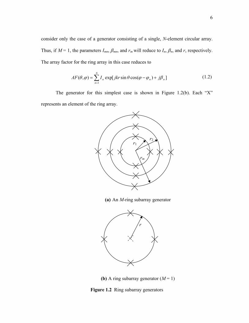
6

consider only the case of a generator consisting of a single, N-element circular array.

Thus, if M = 1, the parameters Imn, βmn, and rm will reduce to In, βn, and r, respectively.

The array factor for the ring array in this case reduces to

])(cossin[exp),(1

nn

N

nn jθjkrIAF βϕϕϕθ +−= ∑

=

(1.2)

The generator for this simplest case is shown in Figure 1.2(b). Each “X”

represents an element of the ring array.

(a) An M-ring subarray generator

(b) A ring subarray generator (M = 1)

Figure 1.2 Ring subarray generators

r1

r

r2

rm

7

Using an algorithm similar to (1.3) in [1], the ring array can be treated as the first stage

of a fractal array. To generate the second stage, the ring array is expanded by a factor

of δ. We then substitute for each antenna element in the expanded array a ring array

identical to that used in the first stage. Thus, we may write

( )( )[ ]∏ ∏= =

−− +Ψ•==2

1

2

1

1112 exp)Ψ()Ψ(

p pnn

pn

p rjIAFAF βδδrrrr

, (1.3)

where

( ) ( ) ( )[ ]( ) ( ) ( )[ ]kjik

kji

ˆcosˆsinsinˆcossin

ˆcosˆsinsinˆcossin2Ψ

θϕθϕθ

θϕθϕθλπ

++=

++=r

(1.4)

and ),Ψ(1

rAF the array factor of the generator (stage 1) in (1.5), can be expressed in

terms of θ and ϕ by

( ) ])(cossin[exp),(),(1

11 nn

N

nn jθjkrIAFAFAF βϕϕϕθϕθ +−===Ψ ∑

=

r (1.5)

This recursive algorithm can be generalized to stage P as

( )( )( )∏ ∏ ∑= = =

−−

+−==P

p

P

p

N

nnn

pn

pP krjIAFAF

1 1 1

111 cossinexp)Ψ()Ψ( βϕϕθδδ

rr (1.6)

By following an analysis identical to that presented in [3], it can be shown that (1.6)

has the highly desirable property of the array factor being self-similar with respect to

frequency as P → ∞. In other words, the array factors are self-similar if the frequency

is multiplied by the similarity factor δ as P → ∞.

As in [2], it can be shown that the radiation characteristics of fractal array

structures are a log-periodic (LP) function of frequency with a log period of δ as

described by (1.7).

8

)Ψ(Ψ(rr

qnormalizednormalized AF)AF δ= (1.7)

This can be interpreted as a frequency shift satisfying (25) in [3]. Thus, if

ff qq δ= (1.8)

where q is an integer, and f is the frequency associated with Ψr

in (1.7), then the array

factor at both frequencies qf and f are equal.

So far, the ideal case where the array has an infinite number of elements has

been discussed. However, all practical arrays have a finite number of elements because

arrays containing an infinite number of elements cannot be constructed in practice.

Equations (1.7) and (1.8) are no longer exact for truncated arrays. However, the array

factor for an ideal fractal antenna array can be approximated by that of a truncated

fractal antenna array. Depending on the generators and the expansion ratio δ, a wide

variety of patterns for fractal antenna arrays can be generated. Several of these patterns

are briefly discussed in the next two sections.

1.1.1 Sierpinski Gasket Array Pattern

Named after Sierpinski, a famous Polish mathematician, the Sierpinski gasket is

one of the basic and most commonly found patterns of fractal geometry [6]. The

Sierpinski Gasket can be constructed through the following four stages.

We start with a blackened, “filled-in” triangle and repeat steps of operation by

first dividing the blackened, “filled-in” triangle into four smaller blackened, “filled-in”

triangles and then, removing the middle triangle as shown in Figure 1.3(a). This is

9

stage 1. We can repeat these steps of operations infinitely to the remaining blackened,

“filled-in” triangles at further stages in the way shown in Figure 1.3(b), (c), and (d).

(a) Stage 1 (b) Stage 2

(c) Stage3 (d) Stage 4

Figure 1.3 Sierpinski gasket

A Sierpinski gasket antenna array can be made using an equilateral triangular

ring array as a generator, with an expansion factor of δ = 2. Several stages in the

growth of the Sierpinski gasket fractal antenna array are shown in Figure 1.4. For

simplicity, assume that all elements on the subarray generator are isotropic, equally

10

excited, and in phase with each other, more precisely speaking, In = 1 and βn = 0 for all

values of n.

Comparing Figure 1.3(a), (b), (c), and (d) to the corresponding Figure 1.4(a),

(b), (c), and (d), respectively, it follows that each element of the array shown in Figure

1.4 can be represented by the corresponding blackened, “filled in” triangle in Figure

1.3. Each element is located at the centroid of the corresponding blackened triangle.

Thus, this configuration is reasonably named the Sierpinski gasket antenna array.

(a) Stage 1 (P = 1) (b) Stage 2 (P = 2)

(c) Stage3 (P = 3) (d) Stage 4 (P = 4)

Figure 1.4 Various stages of growth for the Sierpinski gasket array

11

If we let δ = 2 with three elements in the generator, then (1.6) can be used to

find an expression for the array factor of the pattern, which is given by:

)Ψ2()Ψ( 11

1

rr−

=Π= p

P

pP AFAF (1.9)

If we let In = 1, βn = 0 and N = 3, we can write (1.6) as:

)]3

)1(2(cossin2[exp),( 1

3

1

1∏ ∑= =

−

−−=P

p n

pP

πnθrjkAF ϕϕθ (1.10)

The array factor pattern at ϕ = °0 is shown in Figure 1.5 and Figure 1.6 for various

stages of growth with kr = 3 and kr = 1.5, respectively.

0 10 20 30 40 50 60 70 80 90 100-30

-25

-20

-15

-10

-5

0

theta (degrees)

Mag

nitu

de (d

B)

(a) Stage 1

12

0 10 20 30 40 50 60 70 80 90 100 -30

-25

-20

-15

-10

-5

0

theta (degrees)

Mag

nitu

de (d

B)

(b) Stage 3

0 10 20 30 40 50 60 70 80 90 100 -30

-25

-20

-15

-10

-5

0

theta (degrees)

Mag

nitu

de (d

B)

(c) Stage 5

Figure 1.5 Plot of the Sierpinski gasket array factor for various stages of growth with kr = 3

13

0 10 20 30 40 50 60 70 80 90 100-30

-25

-20

-15

-10

-5

0

theta (degrees)

Mag

nitu

de (d

B)

(a) Stage 1

0

10 20 30

40 50 60 70 80 90

100 -30

-25

-20

-15

-10

-5

0

theta (degrees)

Mag

nitu

de (d

B)

(b) Stage 3

14

(c) Stage 5

Figure 1.6 Plot of the Sierpinski gasket array factor for various stages of growth with kr = 1.5

As can be seen from Figure 1.5 and Figure 1.6, the array factors at kr = 3 and 1.5 tend

to converge to each other as P increases. This agrees with (1.7), meaning that the array

factor of a fractal antenna array is repeated every log-period of δ = 2 as in this

particular case.

1.1.2 Self-Scalable Hexagonal Array Pattern

The self-scalable hexagonal array is generated by an equilateral hexagonal

subarray with an expansion ratio δ = 2. The geometry of the array is shown in Figure

1.7.

0 20 40 60 80 100-30

-25

-20

-15

-10

-5

0

theta (degrees)

Mag

nitu

de (d

B)

15


(c) Stage 3

Figure 1.7 Self-scalable hexagonal antenna array

1

1

1

1

1

1

2

2

1

1

1

1

1

1

2

2

1

1

1

1

1

1

2

2

1

1

1

1

1

11

1

1

1

1

1

11

1

1

1

1

2

2

1

1

1

1

1

2

1

1

2

1

1

3

3

1

1

2

3

2

2

3

2

1

1

1

1

1

1

2

3

3

2

1

1

2

3

3

2

1

1

1

2

2

1

1

1

2

1

2

1

3

3

1

1

3

3

1

2

2

2

2

1

3

3

1

1

3

3

1

2

1

2

1

1

1

2

2

1

1

1

2

3

3

2

1

1

2

3

3

2

1

1

1

1

1

1

2

3

2

2

3

2

1

1

3

3

1

1

2

1

1

2

1

1

1

1

1

2

2

1

1

1

1

11

16

Each of these arrays could also be represented by the scheme illustrated in Figure 1.8,

with elements located on the vertices of each of the hexagons.


(c) Stage 3

Figure 1.8 Figures representing the self-scalable hexagonal antenna array

17

With an appropriate choice of δ = 2, there are some “fictitious” elements which

have other elements stacked on top of them. The number of elements, which are

stacked upon each other at various stages, is shown in Figure 1.7. In reality, each stack

of elements can be represented by a single element; thus the number of physical

elements can be reduced considerably compared with the number of generated or

fictitious elements.

We next consider the array factor characteristics for the self-scalable hexagonal

array. The array factor for a fractal array at stage P (P = 1,2,3,4,5) is given in (1.6),

where

∑=

−−=6

11 )]

6)1(2cos(sinexp[),(

nnjkrAF πϕθϕθ (1.11)

At higher stages, the array factor of the hexagonal array derived from (1.6) and (1.11)

can be represented as:

∏ ∑= =

−

−−=P

p n

pP

πnθrjkδAF1

6

1

1 )]6

)1(2(cossin[exp),( ϕϕθ (1.12)

The array factor given in (1.12) is plotted for the case where °= 0ϕ in Figures 9-13.

18

0 10 20 30 40 50 60 70 80 90 -60

-50

-40

-30

-20

-10

0

theta (degrees)

Mag

nitu

de (d

B)

(a) kr = 6

0 10 20 30 40 50 60 70 80 90 -60

-50

-40

-30

-20

-10

0

theta(degrees)

Mag

nitu

de (d

B)

(b) kr = 3

19

0 10 20 30 40 50 60 70 80 90 -60

-50

-40

-30

-20

-10

0

theta (degrees)

Mag

nitu

de (d

B)

(c) kr = 1.5

Figure 1.9 The array factor pattern of a self-scalable hexagonal array (Stage 1)

0 10 20 30 40 50 60 70 80 90 100-60

-50

-40

-30

-20

-10

0

theta (degrees)

Mag

nitu

de (d

B)

(a) kr = 6

20

0 10 20 30 40 50 60 70 80 90

100 -60

-50

-40

-30

-20

-10

0

theta (degrees)

Mag

nitu

de (d

B)

(b) kr = 3

0 10 20 30 40 50 60 70 80 90 100 -60

-50

-40

-30

-20

-10

0

theta (degrees)

Mag

nitu

de (d

B)

(c) kr = 1.5


21

0 10 20 30 40 50 60 70 80 90 100 -60

-50

-40

-30

-20

-10

0

theta (degrees)

Mag

nitu

de (d

B)

(a) kr = 6

0 10 20 30 40 50 60 70 80 90 100 -60

-50

-40

-30

-20

-10

0

theta (degrees)

Mag

nitu

de (d

B)

(b) kr = 3

22

0 10 20 30 40 50 60 70 80 90 100 -60

-50

-40

-30

-20

-10

0

theta (degrees)

Mag

nitu

de (d

B)

(c) kr = 1.5


0 10 20 30 40 50 60 70 80 90 100 -80

-70

-60

-50

-40

-30

-20

-10

0

theta (degrees)

Mag

nitu

de (d

B)

(a) kr = 6

23

0 10 20 30 40 50 60 70 80 90 100-80

-70

-60

-50

-40

-30

-20

-10

0

theta (degrees)

Mag

nitu

de (d

B)

(b) kr = 3

0 10 20 30 40 50 60 70 80 90 100 -80

-70

-60

-50

-40

-30

-20

-10

0

theta (degrees)

Mag

nitu

de(d

B)

(c) kr = 1.5


24

0 10 20 30 40 50 60 70 80 90 100 -80

-70

-60

-50

-40

-30

-20

-10

0

theta (degrees)

Mag

nitu

de (d

B)

(a) kr = 6

0 10 20 30 40 50 60 70 80 90 100-80

-70

-60

-50

-40

-30

-20

-10

0

theta (degrees)

Mag

nitu

de (d

B)

(b) kr = 3

25

0 10 20 30 40 50 60 70 80 90 100-80

-70

-60

-50

-40

-30

-20

-10

0

theta (degrees)

Mag

nitu

de (d

B)

(c) kr = 1.5


1.2 Some Useful Expressions for the Analysis of Fractal Arrays

This section introduces some mathematical analysis techniques and expressions

that are useful for evaluating the performance of fractal arrays. The results presented

here will be applied to the analysis of fractal arrays throughout this thesis.

1.2.1 Directivity

The directivity of N-element arrays for broadside operation can be determined

by assuming that all individual elements are isotropic. The directivity D for 2-D arrays

may be conveniently expressed in the form (see Appendix for details and derivation):

26

( )( )∑∑∑

∑

=

−

==

=

−

−+

=N

m

m

n mn

mnmn

N

nn

N

nn

rrkrrk

III

ID

2

1

11

2

2

1

sin2 rr

rr (1.13)

and for 3-D arrays

( ) ( )∑∑∑

∑

=

−

==

=

−+−−+−+−

+

=N

m

m

n mn

mnmnmnmnmn

N

nn

N

nn

rrkrrkrrk

III

ID

2

1

11

2

2

1

sinsinrr

rrrr ββββ

(1.14)

where In, nrr and ϕn are the current amplitude excitation, position vector of magnitude rn

and azimuthal angle for the nth element.

1.2.2 Plot of Array Factor in Terms of n or Ψr

The characteristics of the array factor associated with an N- element array of the

form

∑∑==

Ψ•=•=N

nnn

N

nnn rjInrjkInAF

11)exp()ˆexp()ˆ(

rrr (1.15)

can be conveniently illustrated by a plot in terms of n or, more precisely, nx, ny, and nz.

In the case of 2-D arrays, the array factor does not depend on the component nz.

Hence, for this situation, the array factor depends only on nx and ny. The array factor in

27

dB can be represented as a 2-D contour plot. It can be shown (see Appendix A.3) that

the visible region in this case is given by 1≤+ yx nn rr or λπ2

≤Ψ+Ψ yx

rr .

Figure 1.14 Figure to show representation of array factor for 2-D (planar) arrays in terms of nx and ny

Moreover, the polar coordinates ( )ϕρ , are represented by ( )ϕθ ,sin where θ and ϕ are

the vertical and horizontal angles of the far-field point, respectively.

In addition, this representation of the array factor for 2-D arrays not only

illustrates the array factor pattern for a particular minimum spacing dmin, but is also

useful for finding the array factor pattern for various minimum spacings by taking

advantage of the scaling property.

( ) ( )nAFnaAF ˆˆ 21 = (1.16)

nx

ny

(sin θ ,ϕ)

28

where ( )nAF ˆ1 and ( )nAF ˆ2 are the array factors in terms of n with the minimum

spacings dmin = d1 and d2 = ad1, respectively.

By exploiting the translational property, we can calculate the maximum

allowable angle to which the 2-D array can be steered from broadside. To explain the

way in which to calculate the maximum allowable angle θmax, consider a plot of the

array factor in terms of nx and ny. Let us also suppose that the closest high sidelobe

undesirable region is at distance b (1<b<2) away from the origin. Hence, the angle θmax

can be determined by the formula

1sin maxmax−==+ bnn yoxo θ (1.17)

and hence,

( )1arcsinmax −= bθ (1.18)

In the case of 3-D arrays (see Appendix A.4), the array factor depends not only

on nx and ny but also on nz. The visible region is 1ˆ =n or .1=++ zyx nnn rrr It follows

that the spherical coordinates ( )θϕ,,r of the region 1ˆ =n are ( )θϕ,,1 where φ and θ

are the horizontal and vertical angles of the far-field point, respectively. In addition, the

plot of the array factor for a 3-D array can be useful for determining the maximum

allowable angle θmax and array factor pattern for various minimum spacings. However,

the analysis for 3-D arrays is much more complicated than that for 2-D arrays and will

be considered beyond the scope of this thesis. Hence, there is no further discussion on

the analysis using this plot for 3-D arrays.

29

Figure 1.15 Figure to show representation of array factor for 3-D arrays in terms of nx, ny and nz

ny

nz

nx

(1, ϕ, θ )

30

Chapter 2

Fractal Arrays Using Ring Subarray Generators

Associated with the fractal arrays previously discussed, this section presents new

self-scalable pentagonal and octagonal arrays that are generated using 5-element and 8-

element subarray generators respectively. These arrays have the advantage that they can

be recursively generated, allowing development of rapid algorithms for calculating their

radiation patterns. They also possess relatively low sidelobe levels.

2.1 Self-Scalable Pentagonal Arrays

The self-scalable pentagonal array is a fractal array generated by a 5-element ring

subarray generator. Figure 2.1 shows the 5-element ring subarray whose individual

generating elements are located on each of the vertices of a pentagon.

1

1

1

1

1

r

Figure 2.1 5-element ring subarray generator

31

Similar to the case of the self-scalable hexagonal array, the self-scalable pentagonal array

is generated in a way allowing stacking of some of the elements upon each other at

higher stages of growth. Each stack of generated elements can be represented by a single

element. This implementation can reduce the number of real elements, while the current

distribution on the array becomes nonuniform, leading to lower sidelobe levels.

To generate the pentagonal array with a non-uniform current distribution, the

expansion ratio δ is selected in such a way that the generated elements will stack upon

each other. Referring to the geometry shown in Figure 2.2, it follows that:

δrcos 72° + rcos 72° = δr + rcos 144° (2.1)

where

δ = the expansion ratio of the fractal pentagonal antenna array

r = the radius of the 5-element subarray generator

144° 72°

72°

δr

r

dmin

Figure 2.2 Geometry relating expansion ratio δ and dmin for a pentagon subarray generator

32

Consequently, solving (2.1) for δ, yields

δ = 618.172cos1

144 cos-72 cos=

°−°° (2.2)

With this choice of expansion ratio δ, there will be some elements that overlap for higher-

order stages of growth. Each stack of elements could be implemented in practice by using

only one element with excitation current amplitude equal to the sum of the individual

element excitations. The antenna elements shown in Figure 2.3 are represented by dots.

The number adjacent to each element represents the relative excitation current amplitude

on each element.

1

1

1

1

1

1

1 1

1 1

2 1 2

1 2 1

1 2

2 1

1 1 1

1 1


33

1 1 1

2 1 1 1 2 1

1 1 2 1 2 3 2

3 1 13

2 4 1 1 1 4 3 1

3 2 1 2 2 2 2 4 1

1 2 3 2 2 4 1

3 1

2 4 1 1 1 3 3 1 2 3 2

1 1 1 2 1 2 1 1

2 1 1

1 1

(c) Stage 3

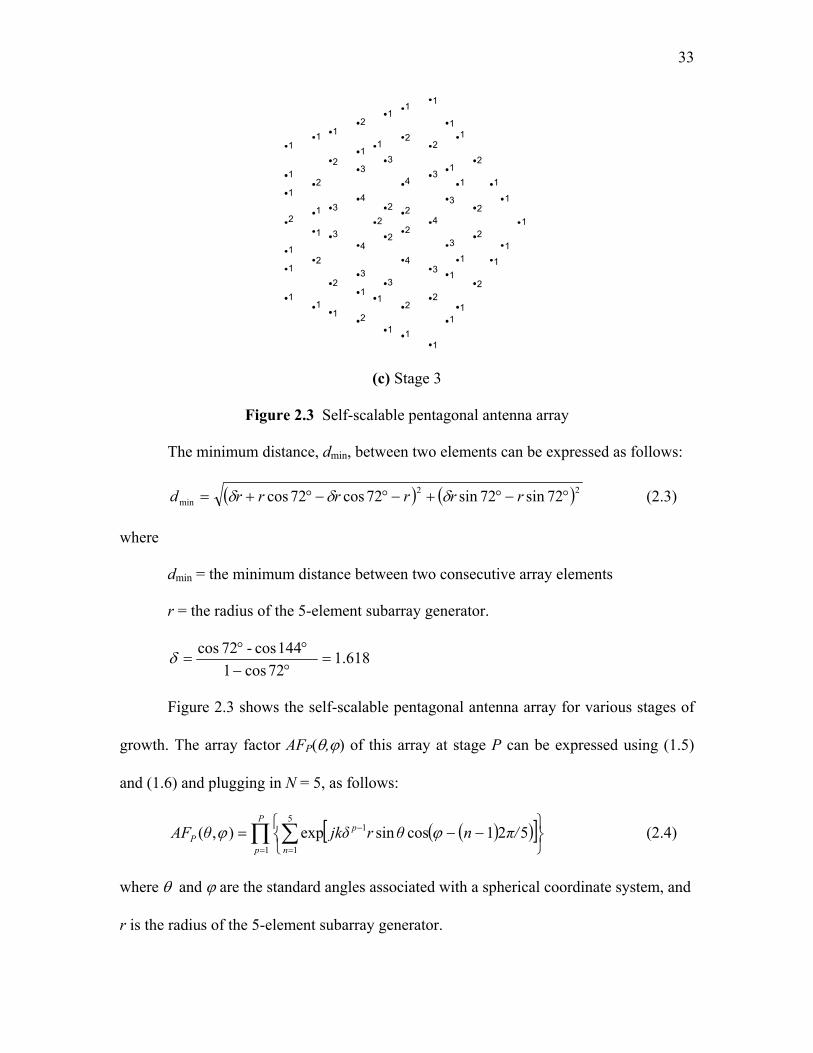
Figure 2.3 Self-scalable pentagonal antenna array

The minimum distance, dmin, between two elements can be expressed as follows:

( ) ( )22min 72sin72sin72cos72cos °−°+−°−°+= rrrrrrd δδδ (2.3)

where

dmin = the minimum distance between two consecutive array elements

r = the radius of the 5-element subarray generator.

618.172cos1

144 cos-72 cos=

°−°°

=δ

Figure 2.3 shows the self-scalable pentagonal antenna array for various stages of

growth. The array factor AFP(θ,ϕ) of this array at stage P can be expressed using (1.5)

and (1.6) and plugging in N = 5, as follows:

( )( )[ ]∏ ∑= =

−

−−=P

p n

pP π/nθrjkδθAF

1

5

1

1 521cossinexp),( ϕϕ (2.4)

where θ and ϕ are the standard angles associated with a spherical coordinate system, and

r is the radius of the 5-element subarray generator.

34

(

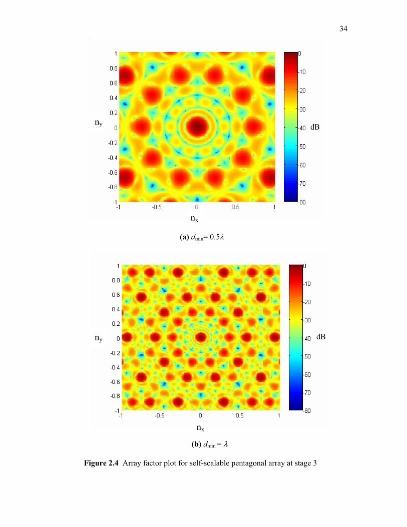
(a) dmin= 0.5λ

(b) dmin = λ

Figure 2.4 Array factor plot for self-scalable pentagonal array at stage 3

nx

ny

ny

nx

dB

dB

35

Figure 2.4(a) and (b) show contour plots of the self-scalable pentagonal array

factor where the x- and y-axes represent nx and ny, respectively. Figure 2.4(a) illustrates

that, with dmin = 0.5λ, sidelobes are low relative to those for dmin = λ shown in Figure

2.4(b). Figure 2.4(b) shows that, with dmin = λ, grating lobes are in the visible region (the

unit circle centered at the origin). In other words, grating lobes are present when dmin = λ.

Slices of the plot for the array factor versus θ with various minimum spacings, dmin =

0.5λ and dmin = λ at a fixed stage 3 are shown in Figure 2.5.

0 10 20 30 40 50 60 70 80 90-45

-40

-35

-30

-25

-20

-15

-10

-5

0

Theta (degrees)

Arra

y Fa

ctor

(dB

)

Figure 2.5 Array factor of the self-scalable stage 3 pentagonal antenna array at stage 3 with minimum spacings of 0.5λ (dashed curve) and λ (solid curve) at ϕ = 0°

Figure 2.5 shows the array factor of the self-scalable pentagonal antenna array for

stage P = 3 evaluated at °= 0ϕ with minimum spacings of 0.5λ and λ. The array factor

36

for the case where dmin = λ is shown by a solid curve whereas for the case where dmin =

0.5λ it is shown by a dashed curve. This figure indicates for both cases that sidelobe

levels are still relatively high compared to the mainbeam.

The sidelobe level of the stage 3 array factor at ϕ = 0° can be reduced by inserting

an element at the center of the subarray generator. Figure 2.6 shows the geometry for the

5-element pentagonal subarray generator with a sixth element added at the origin.

The fractal array generated by this subarray generator at stages 1, 2, and 3 are

shown in Figure 2.7(a), Figure 2.7(b) and Figure 2.7(c), respectively.

1

1

1

1

1

1

r

Figure 2.6 5-element subarray generator modified by inserting an element at the center

37

1

1

1

1

1

1

1

1 1

1 1 1

1 2 1 1

1 2 1

2 1 1 1 1

1 1 2

1 2 1 1

1 1 1

1 1

1


11

12 1 1

11 1 2 1 1

1 1 1 1 21

1 2 1 3 2 1 1 21 3 1

11

1 1 32 2 1 2 5 1 1 1 1 1

11 5 2 1 2 1 3 1 1

1 3 1 1 2 2 11

21 2

2 2 2 2 1 1 5 2 1 1 11 1 2

1 3 1 1 2 2 1 21 5 2 1 2

11 3 1 1

2 2 1 2 5 1 1 1 1 11 1 1 3

1 3 1 11 2 1 3 2 1 1 2

11 1 1 1 2

1 1 2 1 11

2 1 11

11

(c) Stage 3

Figure 2.7 Self-scalable pentagonal array whose subarray generator is modified by inserting one element at the center

The array factor of the modified self-scalable pentagonal antenna array can be expressed

as:

( )( )[ ]∏ ∑= =

−

−−+=P

p n

pP π/nθrjkδθAF

1

5

1

1 521cossinexp1),( ϕϕ (2.5)

38

The minimum spacing dmin of the modified self-scalable pentagonal antenna array

is:

rd =min (2.6)

This differs from the formula that was derived for the self-scalable pentagonal antenna

array given in (2.3).

(a) dmin = 0.5λ

ny

nx

dB

39

ny

(b) dmin = λ

Figure 2.8 Array factor plots for the self-scalable pentagonal array at stage 3 modified by inserting an element at the center of the generator

By comparison with the unmodified case, the plot of array factor for the self-

scalable pentagonal array modified by inserting an element at the center of the generator,

which is illustrated in Figure 2.8(a), has relatively low sidelobes for the case where dmin =

0.5λ. For the case where dmin = λ, as represented in Figure 2.8(b) the plot still has high

sidelobes in the visible region (in the unit circle centered at the origin). Figure 2.9 shows

the array factor of the modified stage 3 self-scalable pentagonal array at °= 0ϕ . The

figure shows that high sidelobe levels remain present in the case where dmin = λ (solid

nx

dB

40

curve). In the case where dmin = 0.5λ (dashed curve) there are no grating lobes present in

the radiation pattern, as represented in Figure 2.8(a) and Figure 2.9.

0 10 20 30 40 50 60 70 80 90 -45

-40

-35

-30

-25

-20

-15

-10

-5

0

Theta (degrees)

Arra

y Fa

ctor

(dB

)

Figure 2.9 The array factor of the stage 3 modified self–scalable pentagonal array for minimum element spacings 0.5λ (dashed curve) and λ (solid curve) at ϕ = 0°

2.2 Self-Scalable Octagonal Arrays

Similar to the case of the self-scalable pentagonal array, the self-scalable

octagonal array is a fractal array generated by a ring subarray generator. The ring

subarray generator in this case is the 8-element subarray shown in Figure 2.10. It is found

that with a certain expansion ratio δ, there will be some stacking of elements causing the

current distribution on the fractal array to be nonuniform. An expression for the

41

expansion ratio δ can be obtained from the geometry illustrated in Figure 2.11. This

expression is given by

δ = cot (22.5°) (2.7)

1

1

1

1

1

1

1

1

r

Figure 2.10 8-element ring subarray generator

δr

r 22.5°

22.5°

dmin

Figure 2.11 Geometry relating to expansion ratio δ and dmin for an octagonal subarray generator

42

Using the expansion ratio given in (2.7), each stack of generated elements can be

implemented as a single physical element by adjusting the excitation currents in the

appropriate way. Also, the minimum spacing between array elements can be expressed

as:

)sin(22.52min °= rd (2.8)

where

dmin = the minimum spacing between real elements

r = the radius of the 8-element subarray generator.

Figure 2.12 shows the pattern of the self-scalable octagonal antenna array with the

expansion ratio, δ = cot 22.5° for several stages P = 1, 2 and 3. Each real element

location is represented by a dot. The figure also shows the relative excitation current

amplitude associated with each element.

The array factor at stage P for the fractal array shown in Figure 2.12 can be

expressed as follows:

( )( )[ ]∏ ∑= =

−

−−=P

p n

pP πnθrjkδθAF

1

8

1

1 4/1cossinexp),( ϕϕ (2.9)

43

1

1 1

1 1

1 1

1

11 1

11 2

1 2

1

1

2 2 1

2

1

11

2 1 2

1

2

1

1

1

1

2

1

2 1 2

1 1

1

2 1

2 2

1

1

21

2 1 1

1 1 1


11 11 1 1 2 2 11 1 21 21 1 11 1 13 1

112 13 33 13 3 1

22

13 21 2 3

2 2

11

2 1 14 2 44 22 12 24

1 121 1

2 3 3 2 1 3

1 13 3 32 31 33 1

332 1 11

3 214

313 1 21 1 1

13 3

44

33

11 2 11 2

3 1

42 1

313 2 12

3 1 3 2 1

11 1

231

21

1

1 1

2 1

3 2 1

1 1 1

2 3 1 3 2 1

231 3 12

41

3211 21

1 3

3 4

43

3 1 1

1 12 1 313 412

31 1

1233 133 13 23 33

1 13 1

2 3 3 2 1 1 2

1 14 2 21 22 44 2 41

12

1 1

22

3 2 12 3

1 2

21

3 3 1 33 31 211131 111 1 12 12 1 1

1 2 2 11 11 11

(c) Stage 3

Figure 2.12 Self-scalable octagonal antenna array

44

(a) dmin = 0.5λ

(b) dmin = λ

Figure 2.13 Array factor plots for the self-scalable octagonal array at stage 3

ny

nx

ny

nx

dB

dB

45

Figures 2.13(a) and (b) show plots of array factor for the self-scalable octagonal

array at Stage 3 in terms of nx (x-axis) and ny (y-axis). Figures 2.13(a) and (b) illustrate

the array factor plot where dmin = 0.5λ and dmin = λ, respectively. Figure 2.13(a) shows

high sidelobes in the visible region while Figure 2.13(b) shows grating lobes in the

visible region, with the unit circle centered at the origin. The grating lobes are higher than

the large sidelobes shown in Figure 2.13(a). This means that relatively high sidelobes

appear for this array in the both cases where dmin = 0.5λ and dmin = λ.

Figure 2.14 shows plots of the array factor pattern of the self-scalable octagonal

antenna array for stage P = 3 evaluated at ϕ = 0° with the minimum spacings between

elements, dmin, of 0.5λ (dashed curve) and λ (solid curve). The figure confirms that there

is at least one high sidelobe in the latter case.

0 10 20 30 40 50 60 70 80 90-80

-70

-60

-50

-40

-30

-20

-10

0

Theta (degrees)

Arra

y Fa

ctor

(dB

)

Figure 2.14 Array factor of the self-scalable stage 3 octagonal antenna array with minimum spacing of 0.5λ (dashed curve) and λ (solid curve) at ϕ = 0°

46

Similar to the self-scalable pentagonal antenna array, the self-scalable octagonal

antenna array can be modified by inserting an element at the center of the subarray

generator, as shown in Figure 2.15(a). The modified self-scalable octagonal antenna array

at stages 1, 2, and 3 are shown in Figure 2.15.

1

1 1

1 1 1

1 1

1

11 1

11 2

1 1 2

1

1

1 2 2 1 1

2

1

11 1

2 1

1 2

1

1

2

1 1

1

1 1 1

1

1 1

2

1

12

1 1

2 1 1

1

1

21

1 2 2 1

1

1

2 11

2 1 1

1 1 1


47

11 11 11 2 1 2 1

1 1 1 21 21 1 1 111

131

112 11 13 33 1 1 13 3

11

12

21

3 2 2 1 11 1 2 2 32

21

11

121

142 11 11 44 22 11 12 24

11

11

1 12

111

1 2 2 3 3 2 2 11

13

1 11

11

133 32 21 31 33

111 11 33

21

113

112

214

313 12 1 2 22 2 1

12 1

13

34

42

23

3 11

22 2 2 212

1 31

211

421

313

1

2 21

1 112

13 11 1 22 31 21 1

12 1

11 1

1

2

13

11

1 11

22

21

1 1 1 1 11

22

21

1 11

13

1

2

11 1

1

1 21

1 12 13 22 1 11 312

11 1

12 2

13

13

124

112

13 1

212 2 2 22

11 3

32

24

43

31

1 21

1 2 22 2 1 21 313

412

211

311

1233 11 11

133 13 12 23 33

11

11

1 13

11

1 2 2 3 3 2 2 11

112

1 11

11

142 21 11 22 44 11 11 24

112

11

11

22

3 2 2 1 11 1 2 2 31

22

11

13 31 1 1 33 31 11 21

113

11

11 1 1 12 12 1 1 11 2 1 2 11 1

1 11

(c) Stage 3

Figure 2.15 Self-scalable octagonal array whose subarray generator is modified by inserting an element at the center The array factor of the modified self-scalable octagonal antenna array can be expressed

as:

( )( )[ ]∏ ∑= =

−

−−+=P

p n

pP πnθrjkδθAF

1

8

1

1 4/1cossinexp1),( ϕϕ (2.10)

The minimum spacing dmin of the modified self-scalable octagonal antenna array is given

by

( )°= 522sin2min .rd (2.11)

48

(a) dmin = 0.5λ

(b) dmin = λ Figure 2.16 Array factor plots for the self-scalable octagonal array at stage 3 inserting an element at the center of the generator

ny

nx

ny

nx

dB

dB

49

Figures 2.16(a) and (b) show plots of the array factor for the self-scalable octagonal array

at Stage 3 modified by inserting an element at the center of the generator in terms of nx

and ny. Figure 2.16(a) shows the array factor plot in the case where dmin = 0.5λ whereas

Figure 2.16(b) illustrates the array factor plot in the case where dmin = λ. Although for

dmin = 0.5λ, the sidelobes are relatively low compared to the large sidelobes for the

unmodified self-scalable octagonal array, for dmin = λ, grating lobes are present in the

visible region. The array factor of the modified self-scalable octagonal array is plotted in

Figure 2.17 for minimum spacings between elements, dmin = 0.5λ (dashed curve) and dmin

= λ (solid curve), evaluated at ϕ = 0°.

Comparing Figure 2.14 to Figure 2.17, the sidelobe level of the stage 3 array

factor of the self-scalable octagonal antenna array with the minimum spacing

0 10 20 30 40 50 60 70 80 90 -80

-70

-60

-50

-40

-30

-20

-10

0

Theta (degrees)

Arra

y Fa

ctor

(dB

)

Figure 2.17 Array factor of the self–scalable octagonal array at stage 3 for ϕ = 0° with minimum spacings of 0.5λ (dashed curve) and λ (solid curve) modified by inserting an element at the center of the generator

50

dmin = 0.5λ at ϕ = 0° is high relative to the mainbeam. While introducing an inserted

element at the center of the subarray generator clearly results in a considerable reduction

in the sidelobe level for a minimum spacing dmin = 0.5λ, no such reduction occurs for

dmin = λ and the maximum directivity for both cases increases as shown in Table 2.1.

Table 2.1 Comparison of maximum directivity for a stage 3 unmodified self-scalable octagonal array and a stage 3 modified self-scalable octagonal array

Maximum Directivity (dB)

Element Spacing

(dmin/λ) Stage 3 Unmodified Self-

Scalable Octagonal Array

Stage 3 Modified Self-

Scalable Octagonal Array

0.5 21.51 26.11

1 23.41 23.90

2.3 Honeycomb Fractal Arrays Honeycomb fractal arrays are generated using ring subarray generators. Like the

self-scalable hexagonal arrays discussed in Chapter 1, honeycomb fractal arrays are also

generated using a 6-element subarray generator. However, unlike the self-scalable

hexagonal array generator, the subarray generator for honeycomb fractal arrays is rotated

by an angle of π /2 from one stage to the next.

The array factor of the honeycomb array may be expressed in the form:

51

( ) ( ) ( )∏ ∑= =

−

−+

−

−=P

p n

pP pnrkjAF

1

6

1

1

21sin

621cosexp),( πθπϕδϕθ (2.12)

where the expansion ratio .3=δ

The honeycomb array at Stage 3 with the associated current amplitude excitation

for each individual element is illustrated in Figure 2.18.

1

1

1

2

1

1

3

2

1

3

3

1

3

3

3

1

2

3

4

1

4

2

3

4

2

4

4

2

1

1

3

4

4

3

4

4

3

4

1

4

4

3

3

4

4

1

4

3

4

4

3

4

4

3

1

1

2

4

4

2

4

3

2

4

1

4

3

2

1

3

3

3

1

3

3

1

2

3

1

1

2

1

1

1

Figure 2.18 Stage 3 honeycomb fractal array

2.3.1 Radiation Characteristics of Honeycomb Fractal Arrays

Figure 2.19 demonstrates that grating lobes are present when the array has a

minimum spacing dmin = λ, since sidelobes with the same intensity as the mainbeam are

present in the visible region (the unit circle centered at the origin). In particular, the

normalized array factor of the Stage 3 honeycomb fractal array sliced at φ = 0° is shown

52

in Figure 2.20. This plot is generated by substituting r = dmin , φ = 0° and P = 3 into

(2.12). Since grating lobes are present, the array is not desirable for broadband

applications which require high directivity. However, for element spacings of dmin = 0.5λ,

the honeycomb array appears to possess relatively low sidelobes.

Figure 2.19 Plot of normalized array factor of the stage 3 honey comb fractal array with dmin = λ

0 10 20 30 40 50 60 70 80 90 -80

-70

-60

-50

-40

-30

-20

-10

0

Theta (degrees)

A

rray

Fac

tor (

dB)

Figure 2.20. Plot of array factor of the stage 3 honeycomb array sliced at ϕ = 0° for dmin = 0.5λ (dashed curve) and dmin = λ (solid curve)

nx

ny dB

53

2.4 Conclusion

Figures 2.4, 2.8, 2.13, and 2.16 show that with the minimum spacing dmin = 0.5λ,

the array factor patterns of the self-scalable pentagonal and self-scalable octagonal array

have relatively low sidelobes, whereas with a minimum spacing dmin = λ, the array factor

patterns of the self-scalable pentagonal and self-scalable octagonal arrays have large

sidelobes.

Next, we make a comparison of Figure 2.4 to Figure 2.8 and Figure 2.13 to Figure

2.16. For the case of the modified self-scalable octagonal array, sidelobes are evidently

lower that those for the unmodified self-scalable octagonal array. However, in the case of

modified self-scalable pentagonal array, with dmin = 0.5λ, the sidelobes are not

significantly lower than those found in the case of the unmodified self-scalable

pentagonal array. However, even for the case where both self-scalable pentagonal and

octagonal arrays are modified by inserting an element at the center of the generators, the

sidelobe levels are still high relative to the mainbeam when the minimum element

spacing is dmin = λ.

Figure 2.19 shows a plot of the normalized array factor of the Stage 3 honey-

comb fractal array whose geometry is illustrated in Figure 2.18. In this case, we see that

high sidelobes are also present in the visible region when the array has a minimum

spacing dmin =λ. However, for element spacings of dmin = 0.5λ, the honeycomb array

appears to possess relatively low sidelobes.

The fractal arrays investigated so far have high sidelobes in the visible region dmin

= λ. This characteristic is undesirable where high directivity is needed for broadband

54

antenna arrays. Because of this, other kinds of fractal arrays will be further investigated

in an effort to identify candidates for broadband operation.

55

Chapter 3

Generalized Principle of Pattern Multiplication and Multiple-Generator Fractal Arrays

The conventional principle of pattern multiplication, which is briefly reviewed in

Section 3.1, is based on the assumption that the subarray generators replacing each

individual element are identical and their orientations are the same. The conventional

principle of pattern multiplication is not adequate for some more complicated array

configurations. Examples of such cases include the Peano and Peano-Gosper curve

arrays, which are discussed in Chapter 4 and 5, respectively. The generalized principle of

pattern multiplication is introduced in Section 3.2, as an effective methodology for

evaluating the radiation patterns produced by these more complex array configurations.

Section 3.3 introduces the array factor expression for fractal arrays generated

using multiple generators, which are discussed extensively in Chapters 4 and 5.

3.1 Conventional Principle of Pattern Multiplication

Initially, let us suppose that there is an antenna array that contains identical

elements, each with the same orientation. The array at the present stage is generated by

replacing each individual elements at the previous stage by a subarray generator whose

individual elements are identical. Also, the orientations of each of the individual elements

are assumed to be the same. Furthermore, the associated array factor of the subarray

generator and the array factor at the pth stage are assumed to be ),( ϕθpb and ),,( ϕθpAF

56

respectively. Hence, the associated array factor of the Pth stage array can be expressed

as:

,),(),(0

∏=

=P

ppP bAF ϕθϕθ (3.1)

3.2 Generalized Principle of Pattern Multiplication As mentioned earlier, the conventional principle of pattern multiplication is not

adequate for applying to more complicated cases where, for each stage, each individual

element is replaced by N different generators (or identical generators with different

orientations). By introducing a matrix ),( ϕθAF defined as:

=

),(...),(.........

),(...),(),(

1

111

ϕθϕθ

ϕθϕθϕθ

NNN

N

AFAF

AFAFAF (3.2)

where ),( ϕθijAF is the array factor associated with the #i element(s) of the subarray

generated by the #j generating element.

In this case, the array factor ),( ϕθAF may be expressed as:

∑∑= =

=N

i

N

jijAFAF

1 1),(),( ϕθϕθ

(3.3)

57

Now, let us suppose that we consider the procedure for generating an array

containing P stages. Further, let us suppose that there is an initiator array containing

generating elements numbered from 1 to N. The array factor, in this case, may be

represented by the matrix ),( ϕθAF introduced in (3.2) as follows:

==

),(000...000),(

),(),(

,0

11,0

00

ϕθ

ϕθϕθϕθ

NNb

bBAF (3.4)

where ),(0 ϕθB is a diagonal matrix. The entry, ),(,0 ϕθiib , is the array factor associated

with the #i generating element(s).

Next, at stage p > 0, we consider replacing each individual #j element with the j

subarray generator. Note that there are N different subarray generators; each of which

contains elements with different numbers 1 to N. The array factors of these N generators,

can be represented by a matrix denoted by ( )ϕθ ,pB , which can be expressed as:

( )

=),(...),(

.........),(...),(

,

,01,

1,11,

ϕθϕθ

ϕθϕθϕθ

NNNp

Npp

p

bb

bbB (3.5)

where the #j column corresponds to the j subarray generator; ),(, ϕθijpb is the array factor

associated with #i elements of the j subarray generator.

58

By applying the conventional principle of pattern multiplication, at stage 1, the

array factor associated with the #i element generated by the #j generating element can be

expressed as:

∑=

=N

kkjikij bbAF

1,0,1,1 ),(),(),( ϕθϕθϕθ (3.6)

or the array factor can be represented in the matrix form:

),(),(),( 011 ϕθϕθϕθ BBAF = (3.7)

By mathematical induction, the array factor matrix representation ),( ϕθPAF can be

expressed as:

),()...,(),(),( 00

ϕθϕθϕθϕθ BBBAF P

P

ppPP ∏

=− == (3.8)

In summary, the array factor is generated using the following procedure:

1. Start with n )( N≤ isotropic elements where b0,ii(θ,ϕ) is the array factor associated with the #i element. Label the #i element with #i. Note that b0,ij(θ,ϕ) = 0, .ji ≠

2. At stage 1, replace the #j element with the subarray whose array factor

associated with the #i element(s) generated by the #j generating element(s) is ).,(,1 ϕθijb

3. At further stages p ),( P≤ replace the #j element(s) with the subarray whose array factor associated with the #i element(s) generated by the #j generating element(s) is ).,(, ϕθijpb

The array factor generated by the procedure outlined above may be expressed as:

59

∑∑= =

=N

i

N

jijPP AFAF

1 1, ),(),( ϕθϕθ (3.9)

where

∏=

−=P

ppPP

0

),(),( ϕθϕθ BAF

3.3 Fractal Arrays Generated by Multiple Generators

The fractal arrays discussed in Chapter 1 are generated using ring subarray

generators. Due to their geometrical complexity, the conventional principle of pattern

multiplication may not be applied in these cases. Instead, the array factor expression for

more complex-structured antenna arrays may be written as a summation of all elements

of a matrix ),( ϕθAF as follows:

∑∑= =

=N

i

N

jAFAF

1 1),(),( ϕθϕθ ij (3.10)

where the array factor matrix representation ),( ϕθAF is of the form:

( )∏−=

−−−−

−−− ΨΨΨ=Ψ=

2

1

22

2)()()()(),( 11

)1(1

1

P

Pp

Ppp

PP δδδϕθ αα cfaAFAF (3.11)

where

60

( )

=Ψ−−−

NN

PP

a

aa

...000...000...00...0

)( 22

11

112

δαa and

=Ψ−

NN

P

c

cc

...000...000...00...0

)( 22

11

12δc

are diagonal matrices. The ith diagonal entry aii of the matrix ( ) )( 112

Ψ−−−

PP δαa is the array

factor of a subarray generated by the #i element and the jth diagonal entry cjj of the matrix

)( 12 Ψ−Pδc is the array factor of a subarray associated with the jth initiator element. The

term )( 1)1( Ψ−

−−p

p δαf is a matrix; the entry of the ith row and the jth column, fij, is the

array factor of a subarray of #i elements replacing the #j element. Also, note that the

subscript –(p-1)α means that the all subarrays are rotated clockwise by an angle of

(p-1)α.

If we set P1 = 0 and P2 = P, then, the matrix representation for ( )ϕθ ,AF can be

expressed as:

( )∏=

−−−−

−−− ΨΨΨ=Ψ=

P

p

Ppp

PP

0

11)1(

11 )()()()(),( δδδϕθ αα cfaAFAF (3.12)

where P represents the stage of the associated fractal array. By some mathematical

manipulation, the array factor can be expressed in the form

P

P

ppP CFACBAAF PPP

== ∏

=0

),( ϕθ (3.13)

where

[ ] [ ]NNN aaaa .............. 111 ==A (3.14)

61

=

NNN

N

p

ff

ff

..............................

......

1

111

F , and (3.15)

=

=

NNN

P

c

c

c

c

...

.........

111

C (3.16)

Also, note that ai and ci are the diagonal entries of the matrices ( ) )( 11 Ψ−−−

Pp δαa

and )( 1Ψ−Pδc , respectively, and fij is the entry of the ith row and jth column of

)( 1)1( Ψ−

−−p

p δαf .

The array factor formulations discussed so far in this section are expressed in

general terms. Specific applications of this generalized principle of pattern multiplication

will be considered in detail for the Peano and Peano-Gosper fractal arrays discussed in

Chapters 4 and 5, respectively.

62

Chapter 4

Peano and Sierpinski Dragon Fractal Arrays

Motivated by a fractal curve, known as the Peano Curve, each element of the

Peano fractal array is located at equally spaced intervals along the curve. Peano curves

are more complicated than the type of fractals discussed in the first two chapters. The

initiator for Peano curves is a straight line segment. Also, they have two generators rather

than one. Each generator is identical in shape but different in orientation.

4.1 Construction of the Peano Curve

The Peano curve may be constructed by following the steps outline below [4]:

1. Start with the horizontal initiator (i.e., the line segment of the unit length) shown

in Figure 4.1(a)

1

Figure 4.1(a) Initiator of the Peano curve

63

2. At stage 1, replace the initiator with the generator shown in Figure 4.1(b)

1

31

31

31

31

Figure 4.1(b) Generator for the horizontal generating line

3. At stage 2, replace all the generated horizontal lines at the previous stage with the generator shown in Figure 4.1(b) scaled by the factor of s =1/3, and replace all the generated vertical lines at the previous stage with the generator shown in Figure 4.1(c) scaled by the factor of s =1/3.

64

31

1

31

31

31

Figure 4.1(c) Generator for the vertical generating line

65

4. For further stages, repeat step 3.

Figure 4.1(a) shows the initiator of the Peano Curve. By replacing the initiator

with the generator shown in Figure 4.1(b), the Peano Curve at stage 1 is obtained as

shown in Figure 4.2(a) whereas the Peano curve at stage 2 is shown in Figure 4.2(b).

1

31

31

31

31

Figure 4.2(a) Peano curve (at stage 1)

66

31

31

31

1

31

91

Figure 4.2(b) Peano curve (at stage 2)

As mentioned earlier, Peano curves are more complicated than the fractal curves

discussed in the first two chapters. The curves have two generators; each of which is

identical in shape but different in orientation.

4.2 Construction of Peano Fractal Arrays

The steps in the construction of the Peano fractal array are listed below:

1. Start with an initiator element associated with the horizontal line initiator of the Peano curve. Label it “ # 1” as shown in Figure 4.3.

67

#1

dmin

Figure 4.3 Initiator element of the Peano curve array

The array factor may be described as

.1),( =ϕθAF (4.1)

At stage 1, replace the initiator element in the previous step with the subarray generator as shown in Figure 4.4.

#1

#1

#1

#1

#2

# 2

#1

dmin

#2

#2

dmin dmin

dmin

dmin

Figure 4.4 Subarray generator of the Peano curve array

Label each element of the subarray generator associated with the horizontal generated line with “#1” and each element of the subarray generator associated with the vertical generated line with “#2” (not available at stage 1). Now, the generated elements at the previous stage become the generating elements at the present stage. The array factor can be described as

68

),(),(2

1i11, ϕϕ θfθAF

i∑=

= , (4.2)

where ),θ(, ϕijpf , the entry of fp ),( ϕθ in the ith row and jth column, is the array factor of the subarray due to the #i generated elements replacing each of the #j generating elements, expanded by the expansion ratio of 3p-1. Hence, the array factor ),( ϕθAF can be rewritten as

),(),θ(2

1

2

1ϕϕ θAFAF

i jji,∑∑

= =

= , (4.3)

where

=

0001

),(),(),(),(

),θ(22,121,1

12,111,1

ϕϕϕϕ

ϕθfθfθfθf

AF

The terms f1,11(θ,φ) and f1,21(θ,φ) are illustrated by Figure 4.5 by letting p = 1.

2. At step 2, expand the array at the previous stage with the expansion ratio of δ = 3 and replace each of the #1 generating elements at the previous stage with the subarray shown in Figure 4.4 and each of the #2 generating elements with the subarray generator shown in Figure 4.4 rotated by 90°. Label each element of the subarray generator associated with the horizontal generated line with “#1” and each element of the subarray generator associated with the vertical generated line with “#2”. Now, the generated elements at the previous stage become the generating elements in the present stage. Hence, the array factor AF(θ,ϕ) can be represented by (4.3), where

=

0001

),(),(),(),(

),(),(),(),(

),θ(22,221,2

12,211,2

22,121,1

12,111,1

ϕϕϕϕ

ϕϕϕϕ

ϕθfθfθfθf

θfθfθfθf

AF (4.4)

69

#1 #1

#1

#1

#1

δ p-1dmin δ p-1dmin δ p-1dmin

δ p-1dmin

δ p-1dmin

#2

# 2

dmin

#2

#2

dmin dmin

δ p-1dmin

δ p-1dmin

),(),(),(),(

p,22p,21

p,12p,11

ϕϕϕϕ

θfθfθfθf

Figure 4.5 Figure to illustrate fp,11(θ,φ) and fp,21(θ,φ)

70

3. At step 2, expand the array at the previous stage with the expansion ratio of δ = 3 and replace each of the #1 generating elements at the previous stage with the subarray shown in Fig. 4.4 and each of the #2 generating elements with the subarray generator shown in Fig. 4.4 rotated by 90°. Label each element of the subarray generator associated with the horizontal generated line with “#1” and each element of the subarray generator associated with the vertical generated line with “#2”. Now, the generated elements at the previous stage become the generating elements in the present stage. Hence, the array factor AF(θ,ϕ) can be represented by (4.3), where

=

0001

),(),(),(),(

),(),(),(),(

),(22,221,2

12,211,2

22,121,1

12,111,1

ϕϕϕϕ

ϕϕϕϕ

ϕθfθfθfθf

θfθfθfθf

θAF (4.4)

4. Repeat step 2 for further stages. Consequently, AF(θ,ϕ) can be represented by (4.3), where

=∏

= 0001

),(),(),(),(

)(1 22,21,

12,11,P

p pp

pp

θfθfθfθf

θ,ϕϕϕϕ

ϕAF (4.5)

5. In the final step, replace the #1 element with two antenna elements aligned horizontally and the #2 element with two antenna elements aligned vertically. Similar to the previous step, the array factor AF(θ,ϕ) can be represented by (4.3), where

( ) ( )( ) ( )

=

=

∏

∏

=

=

ϕθϕθϕθϕθ

ϕϕϕϕ

ϕϕ

ϕϕϕϕ

ϕϕ

ϕ

,,,,

),(),(),(),(

),(00),(

0001

),(),(),(),(

),(00),(

),(

2221

1211

1 22,21,

12,11,

22

11

1 22,21,

12,11,

22

11

cccc

θfθfθfθf

θaθa

θfθfθfθf

θaθa

θ

P

p pp

pp

P

p pp

ppAF

(4.6)

a11 ),( ϕθ = the array factor associated with the horizontal 2-element subarray replacing each of the #1 (horizontal) generated elements.

a22 ),( ϕθ = the array factor associated with the vertical 2-element subarray

replacing each of the #2 (vertical) generated elements.

c(θ,ϕ) =

0001

71

In summary, the array factor at stage P, AFP(θ,ϕ) can be written as:

∑∑= =

=2

1

2

1),(),(

i jP θAFθAF ϕϕ P,ij (4.7)

where

),(),(),θ(),(1

ϕϕϕϕ θθθP

ppP cfaAF ∏

=

= (4.8)

The matrix )( ϕθ,PAF represents the array factor of the stage P Peano curve array. Its

elements )( ϕθ,ijP,AF are the array factor of the subarray generators due to the #i

generator element generated by the #j generating element.

The 2x2 diagonal matrix a(θ,ϕ) is given by

a ),( ϕθ =

),(0

0),(

22

11

ϕϕ

θaθa

(4.9)

It represents the array factors of the 2-element subarray generators, where a11 ),( ϕθ is the

array factor associated with the horizontal 2-element subarray replacing each of the #1

(horizontal) generated elements. Similarly, a22 ),( ϕθ is the array factor associated with

the vertical 2-element subarray replacing each of the #2 (vertical) generated elements.

fp,i,j ),( ϕθ , the entry of fp ),( ϕθ in the ith row and jth column, is the array factor of the

subarray due to the #i generated elements replacing each of the #j generating elements,

expanded by the expansion ratio of 3p-1. Finally,

c ),( ϕθ =( ) ( )( ) ( )

=

0001

,,,,

2221

1211

ϕθϕθϕθϕθ

cccc

(4.10)

is the diagonal matrix that represents the array factor of the initiator element(s). In this

case, the procedure starts with only a single #1 initiator element assumed to be isotropic.

72

In this case, there is only one non-zero constant entry assumed to be one in the first row

and column. The expression for ),( ϕθAF given in (4.6) may be rewritten as follows:

(4.11)000),(

),(),(),(),(

),(00),(

),( 11

1 22,21,

12,11,

22

11

= ∏

=

ϕϕϕϕϕ

ϕϕ

ϕθc

θfθfθfθf

θaθa

θP

p pp

ppAF

By rearranging (4.9), it follows that (4.7) can be expressed in the form:

[ ]

= ∏

= 0),θ(

),θ(),θ(),θ(),θ(

),θ(),θ()( 11

1 p,22p,21

p,12p,112211

ϕϕϕϕϕ

ϕϕϕc

ffff

aaθ,AFP

pP (4.12)

Using the following substitutions:

( )

= ϕθϕθ cossin

2cos2, min

11dka (4.13)

( )

−=

2cossin

2cos2, min

22πϕθϕθ

dka (4.14)

[ ] [ ][ ] [ ]

=

2,21,22,11,1

,,,,

2221

1211

)(θf)(θf)(θf)(θf

p,p,

p,p,

ϕϕϕϕ

(4.15)

73

where

( )

( )

( )

( )

≠

−+++

−+−

=

−+−+

−++

=

−

−

−

−

jijdk

jdk

jijdk

jdk

ji

p

p

p

p

,2

14

cossin2

2cos2

21

4cossin

22cos2

,2

12

cossin2

cos2

21cossin

2cos21

],[

min1

min1

min1

min1

ππϕθδ

ππϕθδ

ππϕθδ

πϕθδ

(4.16)

and

==

=otherwise. 0,

1ji ,1),( ϕθijc (4.17)

Now, the array factor is of the form (3.13), where

CFACAB PP

== ∏

=

P

pAF

0

),( ϕθ (4.18)

where

( ) [ ] ( ) ( )[ ]ϕθϕθϕθ ,, 221121 aaaa === ,aA (4.19)

( ) ( )( ) ( )

[ ] [ ][ ] [ ]

=

=

=

2,21,22,11,1

,,,,

2221

1211

2221

1211

ϕθϕθϕθϕθ

ffff

ffff

pF , and (4.20)

( ) ( )( )

=

=

==

01

,,

,22

11

2

1

ϕθϕθ

ϕθcc

cc

cC . (4.21)

74

An example of construction of the Peano curve array at stage 2 is shown in Figure

4.6. Also, the Peano fractal array at stages P = 1 and 2 are shown in Figure 4.7

#1

dmin

Figure 4.6(a) Construction of the Peano fractal array (at step 1)

#1 #1

#1

#1

#2 #2

#2 #2

#1

dmin

dmin

dmin

dmin dmin

Figure 4.6(b) Construction of the Peano fractal array (at step 2)

75

#1 #1

#1

#1

#2 #2

#2 #2 #1 #1 #1

#1

#1

#2 #2

#2 #2 #1

#1 #1

#1

#1

#2 #2

#2 #2 #1

#1 #1

#1

#1

#2 #2

#2 #2 #1

#2

#2 #2 #2 #1

#1

#1

#1 #2

#2

#2 #2 #2 #1

#1

#1

#1 #2

#2

#2 #2 #2 #1

#1

#1

#1 #2

#2

#2 #2 #2 #1

#1

#1

#1 #2

#1 #1

#1

#1

#2 #2

#2 #2 #1

dmin

3dmin 3dmin

3dmin

3dmin

3dmin

Figure 4.6(c) Construction of the Peano fractal array (at step 3)

1

2

4

2

2

4

4

4

2

2

4

4

4

4

4

2

2

4

4

4

4

4

4

42

2

4

4

4

4

4

4

4 2

2

4

4

4

4

4

2

2

4

4

4

2

2

4

2

1

dmin 3dmin 3dmin dmin dmin

3dmin

3dmin

dmin

dmin

Figure 4.6(d) Construction of the Stage 2 Peano fractal array (at step 4)

76

1

2

4

2

2

4

2

1

dmin

3dmin

dmin

dmin

dmin dmin

Figure 4.7(a) Peano fractal array (at stage 1)

77

1

2

4

2

2

4

4

4

2

2

4

4

4

4

4

2

2

4

4

4

4

4

4

42

2

4

4

4

4

4

4

4 2

2

4

4

4

4

4

2

2

4

4

4

2

2

4

2

1

dmin 3dmin 3dmin dmin dmin

3dmin

3dmin

dmin

dmin

Figure 4.7(b) Peano fractal array (at stage 2)

Figure 4.8 illustrates a plot of the array factor as a function of nx and ny for the

stage 3 Peano fractal array with minimum spacing dmin = λ. The plot shows that grating

lobes are present in the visible region. Figure 4.9 shows the array factor of the Peano

fractal array at stage P = 3 with the minimum spacing between elements dmin = 0.5λ and λ

at ϕ = 0°. While no grating lobes are present in the half wavelength spaced case,

relatively high sidelobes (grating lobes) are evident in the full wavelength spaced case.

Hence, this array may not be suitable for broadband applications.

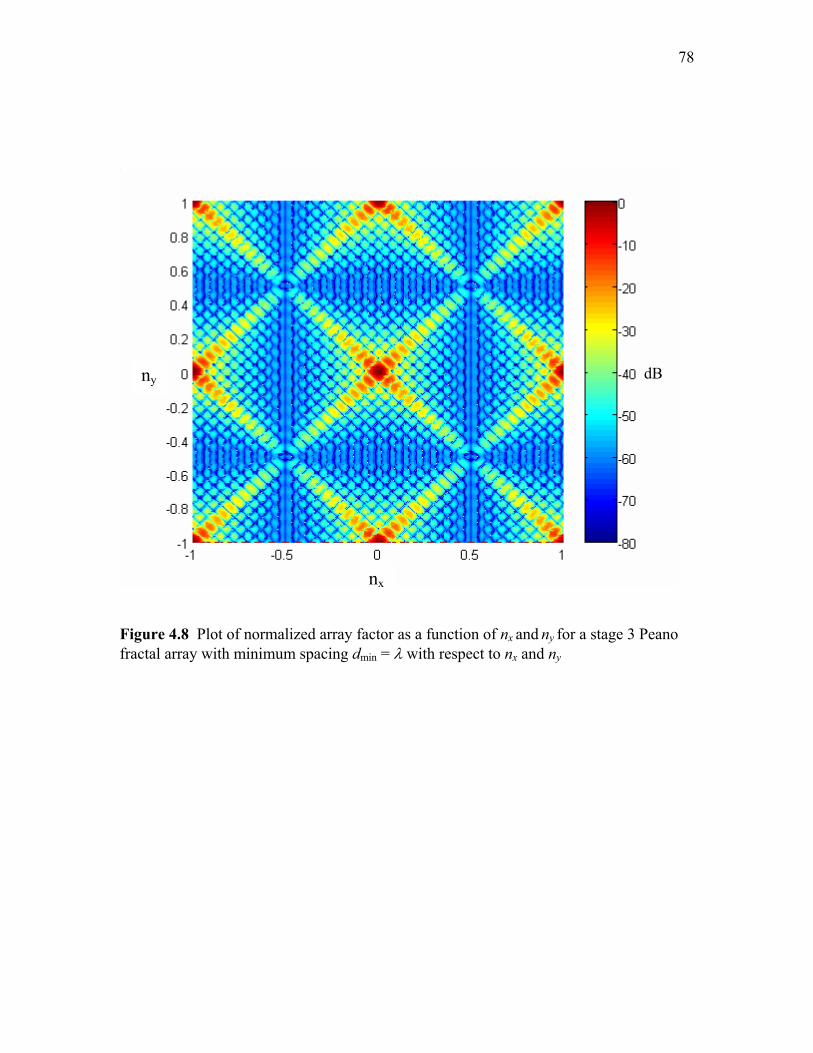
78

Figure 4.8 Plot of normalized array factor as a function of nx and ny for a stage 3 Peano fractal array with minimum spacing dmin = λ with respect to nx and ny

ny

nx

dB

79

0 10 20 30 40 50 60 70 80 90 -80

-70

-60

-50

-40

-30

-20

-10

0

Theta (degrees)

Arra

y Fa

ctor

(dB)

Figure 4.9 Normalized array factor of the Peano curve array at °= 0ϕ , stage 3, dmin = 0.5λ (dashed curve) and dmin = λ (solid curve)

4.3 The Construction of Sierpinski Dragon Array

In this section we will consider a new type of fractal array, which we call the

Sierpinski dragon array. The steps in the generation of the Sierpinski dragon fractal curve

are summarized below [53]:

1. Start with the initiator (line segment) show in Figure 4.10(a).

2. At stage 1, replace the initiator by the generator shown in Figure 4.10(b). Hence, the generator becomes the Sierpinski dragon curve at stage 1.

80

3. For further stages, replace each individual line by the generator shown, in Figure 4.10(b), which is scaled by a factor s = 1/2 and rotated by angles corresponding to Figure 4.10(c), which shows Sierpinski dragon curves superimposed for stages P = 1, 2 and 3.

Figure 4.10(a) Initiator of Sierpinski dragon

Figure 4.10(b) Stage 1 Sierpinski dragon curve, generator is shown by solid curve, whereas the dashed line represents the initiator

Figure 4.10(c) Construction of the Sierpinski dragon curve (stage 2)

4. Generate higher order Sierpinski dragon curves by a replication of the iterative process describe in step 3.

81

Figure 4.11 shows the Sierpinski dragon curves for stages 1, 3, and 5.


(c) Stage 5

Figure 4.11 Sierpinski dragon

82

4.4 The Sierpinski Dragon Array

Similar to the Peano fractal array discussed earlier, the Sierpinski dragon fractal

array may be constructed by a procedure which is similar to that of the Peano fractal

array. The associated array factor ),( ϕθPAF may be expressed as:

CFACAB pP

== ∏

=

P

pPAF

0

),( ϕθ (4.22)

where

[ ]61 ... aa=A (4.23)

=pp

pp

ff

ff

6661

1611

............

...

pF (4.24)

=

0...01

C (4.25)

( )

−= iikda ϕϕθ cossin

2cos2 min (4.26)

6

2)1( πϕ −= ii (4.27)

83

P1pp FFF

= ∏∏

−

=−

=

1

11

P

p

P

p (4.28)

[ ])66( x

pijf=pF (4.29)

[ ]∑∈

−−=ijNn

njnpp

ij krjf ]cos[sinexp γϕϕθ (4.30)

221nn

pnp yxr += −δ (4.31)

<+

=

>

=

0,arctan

0,0

0,arctan

nn

n

n

nn

n

n

xxy

x

xxy

π

γ (4.32)

62)1( πϕ −= jj (4.33)

2=δ (4.34)

84

[ ]

{ } { } { }{ } { } { }

{ } { } { }{ } { } { }

{ } { } { }{ } { } { }

==

231231

123123

312312

)66(

φφφφφφ

φφφφφφ

φφφφφφ

xijNN (4.35)

Table 4.1 The parameters xn and yn expressed in terms of dmin

n

xn

yn

1 2mind

− min83 d

2 0 min4

3 d

3 2mind min8

3 d

The geometry for the Sierpinski dragon array at stages P = 3 and 5 is illustrated in

Figure 4.12.

85

1

2 2

2

2

2

2

2

2

2

2

2

2

2

2

2

2

2

2

2

2

2

2

2

2

2

2

1

Figure 4.12(a) The stage 3 Sierpinski dragon array

12 2

2

2

2

2

2

2

2

2

2

2

2

2

2

2

2

2

2

2

2

2

2

2

2

2

2

2

2

2

2

2

2

2

2

2

2

2

2

2

2

2

2

2

2

2

2

2

2

2

2

2

2

2

2

2

2

2

2

2

2

2

2

2

2

2

2

2

2

2

2

2

2

2

2

2

2

2

2

2

2

2

2

2

2

2

2

2

2

2

2

2

2

2

2

2

2

2

2

2

2

2

2

2

2

2

2

2

2

2

2

2

2

2

2

2

2

2

2

2

2

22

2

2

2

2

2

2

2

2

2

2

2

2

2

2

2

2

2

2

2

2

2

2

2

2

2

2

2

2

2

2

2

2

2

2

2

2

2

2

2

2

2

2

2

2

2

2

2

2

2

2

2

2

2

2

2

2

2

2

2

2

2

2

2

2

2

2

2

2

2

2

2

2

2

2

2

2

2

2

2

2

2

2

2

2

2

2

2

2

2

2

2

2

2

2

2

2

2

2

2

2

2

2

2

2

2

2

2

2

2

2

2

2

2

2

2

2

2

2

21

Figure 4.12(b) The stage 5 Sierpinski dragon array

86

Figure 4.13 Plot of the normalized Sierpinski dragon array factor at stage 5 with dmin = λ with respect to nx and ny

Figure 4.13 shows a plot of the normalized array factor. The x- and y-axes denote

ϕθ cossin=xn and ϕθ sinsin=yn . This figure demonstrates that high sidelobes are

present in the visible region when λ=mind since red spots, which represent high sidelobe

levels, are located inside the unit circle centered at the origin. In particular, plots of the

normalized array factor versus θ of the stage 3 and stage 5 Sierpinski dragon array with

dmin = 0.5λ and λ sliced at ϕ = 0° are shown in Figures 4.14 and 4.15, respectively.

These figures also demonstrate that high sidelobe levels are present when the minimum

spacing dmin = λ. This characteristic is not desirable for broadband applications.

nx

ny dB

87

0 10 20 30 40 50 60 70 80 90-80

-70

-60

-50

-40

-30

-20

-10

0

Theta (degrees)

Arr

ay F

acto

r (dB

)

Figure 4.14 Plot of stage 3 Sierpinski dragon normalized array factor for ϕ = 0° with minimum spacings of dmin = λ (solid curve) and dmin = 0.5λ (dashed curve)

88

0 10 20 30 40 50 60 70 80 90-80

-70

-60

-50

-40

-30

-20

-10

0

Theta (degrees)

Arr

ay F

acto

r (dB

)

Figure 4.15 Plot of stage 5 Sierpinski dragon normalized array factor for ϕ = 0° for minimum spacings of dmin = λ (solid curve) and dmin = 0.5λ (dashed curve)

89

Chapter 5

The Peano-Gosper Fractal Array

Fractal concepts were first introduced for use in antenna array theory by Kim and

Jaggard [41] who developed a design methodology for quasi-random arrays that is based

on properties of random fractals. In other words, random fractals were used to generate

array configurations that are somewhere between completely ordered, i.e., periodic, and

completely disordered, or random. The main advantage of this technique is that it yields

sparse arrays that possess relatively low sidelobes, a feature typically associated with

periodic arrays but not random arrays. They are also robust, with respect to element

failure, a feature which is typically associated with random arrays but not periodic arrays.

More recently, the fact that deterministic fractal arrays can be generated recursively, i.e.,

through successive stages of growth starting from a simple generating array, was

exploited by Werner et al. [48]. It is discussed earlier in the thesis in Chapters 1-3 in

order to develop rapid algorithms for use in efficient radiation pattern computations and

adaptive beamforming, especially for arrays with multiple stages of growth that contain a

relatively large number of elements. It was also demonstrated in [48] that fractal arrays

generated in this recursive fashion are examples of deterministically thinned arrays. A

more comprehensive overview of these and other topics related to the theory and design

of fractal arrays may be found in [49].

Techniques based on simulated annealing and genetic algorithms have been

investigated for optimization of thinned arrays [54-58]. A typical scenario involves

optimizing an array configuration to yield the lowest possible sidelobe levels by starting

90

with a fully populated uniformly spaced array and either removing certain elements or

perturbing the existing element locations. Genetic algorithm techniques have been

developed in [59-61] for evolving thinned aperiodic phased arrays with reduced grating

lobes when steered over large scan angles. The optimization procedures introduced in

[54-58] have proven to be extremely versatile and robust design tools. However, one of

the main drawbacks in these cases is that the design process is not based on simple

deterministic design rules and leads to arrays with non-uniformly spaced elements.

In this chapter the radiation properties of a new class of deterministic fractal

arrays are investigated whose geometry is based on self-avoiding Peano-Gosper curves.

5.1 Construction of Peano-Gosper Curves

The procedure to construct the Peano-Gosper curve is described as follows [1]:

1. Start with the same initiator as the Peano curve shown in Figure 5.1.

1

Figure 5.1 The Peano-Gosper curve initiator

2. At Stage 1, replace the initiator with the generator shown in Figure 5.2.

3. At Stage 2, turn the generator counterclockwise as shown in Figure 5.2 until the link between both ends is aligned in the same direction as that of each line segment of the generator(s) in the previous stage. Scale the generator until the size of the links at both ends is the same as that of each line segment of the generator. Replace each line segment of the generated curve at the previous stage with an appropriately scaled version of the generator.

4. Repeat step 3 for further stages.

91

1

d

α

60°-α

60°

α

Figure 5.2 The Peano-Gosper curve generator


92

Figure 5.3 The first three stages in the construction of a self-avoiding Peano-Gosper curve. The initiator is shown as the dashed line superimposed on the stage 1 generator. The generator (unscaled) is shown again in (b) as the dashed curve superimposed on the Stage 2 Peano-Gosper curve

The first three stages in the construction of a Peano-Gosper curve are shown in

Figure 5.3 [1]. Figure 5.4 shows stages 1, 2, and 4 Gosper islands bounding the

associated Peano-Gosper curves which fill the interior. The boundary contour of these

Gosper islands are formed by a variant of a closed Koch curve. One of the notable

features of Gosper islands is that they can be used to cover the plane via a tiling [1].

Furthermore, Gosper island tiles are self-similar and can be divided into seven smaller

tiles, each representing a scaled copy of the original. This property is known as pertiling.

(c) Stage 3

93


(c) Stage 4 Figure 5.4 Gosper islands and their corresponding Peano-Gosper curves for (a) stage 1, (b) stage 2, and (c) stage 4

5.2 Construction of the Peano-Gosper Fractal Array

The first three stages (i.e., P=1, P=2, and P=3) in the construction of a fractal

array based on the Peano-Gosper curve are shown in Figure 5.5.

94

1

2

2

2

2

2

2

1

1

2

2

2

2

2

2

2

2

2

2

2

2

2

2

2

2

2

2

2

2

2

2

2

2

2

2

2

2

2

2

2

2

2

2

2

2

2

2

2

2

2

2

2

2

2

2

1

2

2

2

2

2

1

2

2

2

2

2

2

2

2

2

2

2

2

2

2

2

2

2

2

2

2

2

2

2

2

2

2

2

2

2

2

2

2

2

2

2

2

2

2

2

2

2

2

2

2

2

2

2

2

2

2

2

2

2

2

2

2

2

2

2

2

2

2

2

2

2

2

2

2

2

2

2

2

2

2

2

2

2

2

2

2

2

2

2

2

2

2

2

2

2

2

2

2

2

2

2

2

2

2

2

2

2

2

2

2

2

2

2

2

2

2

2

2

2

2

2

2

2

2

2

2

2

2

2

2

2

2

2

2

2

2

2

2

2

2

2

2

2

2

2

2

2

2

2

2

2

2

2

2

2

2

2

2

2

2

2

2

2

2

2

2

2

2

2

2

2

2

2

2

2

2

2

2

2

2

2

2

2

2

2

2

2

2

2

2

2

2

2

2

2

2

2

2

2

2

2

2

2

2

2

2

2

2

2

2

2

2

2

2

2

2

2

2

2

2

2

2

2

2

2

2

2

2

2

2

2

2

2

2

2

2

2

2

2

2

2

2

2

2

2

2

2

2

2

2

2

2

2

2

2

2

2

2

2

2

2

2

2

2

2

2

2

2

2

2

2

2

2

2

2

2

2

2

2

2

2

2

2

2

2

2

2

2

2

2

2

2

2

2

2

2

2

2

2

2

2

2

2

2

2

2

2

2

2

2

2

2

2

2

2

2

2

2

2

2

2

2

2

2

2

2

2

2

2

2

2

2

2

2

2

2

2

2

2

2

2

1

2

2

2

2

Figure 5.5 Element locations and associated current distribution for Stages 1-3 Peano-Gosper fractal arrays with minimum spacing between elements and expansion factor denoted by mind and ,δ respectively. Note that the spacing mind between consecutive array elements along the Peano-Gosper curve is assumed to be the same for each stage.


(c) Stage 3

95

Also indicated in Figure 5.5 are the location of the elements and their corresponding

values of current amplitude excitation. The minimum spacing between array elements is

assumed to be held fixed at a value of mind for each stage of growth.

The procedure to construct the fractal array associated with the Peano-Gosper curve

is as follows:

1. Start with an initiator element. Label it “#1”. The array factor AF(θ,ϕ) in this case for a single isotropic source can be written as:

.1),θ( =ϕAF (5.1)

2. At stage 1, replace the initiator with the generated elements corresponding to the #1 generating element shown in Figure 5.6.

#1

#2

#3

#4

#5

#6

#7

α α 60°-α

60°

ddδd min

min =

dmin

rn

ϕn

Figure 5.6 Generating elements with n = 1 to n = 7 are located along the stage 1 Peano-Gosper curve

96

3. Similar to the case considered previously for the Peano curve array, the array factor AF(θ,ϕ) can be expressed as:

,),(),(3

1

3

1,∑∑

= =

=i j

jiAFAF ϕθϕθ (5.2)

where

cfAF 1=),( ϕθ

Also similar to the case of the Peano curve array, 1f = ( ) ,1 ϕθf = [f1,i,j( )ϕθ, ]3x3 is the matrix that represents the array factor of the subarray generators. The expression f1,i,j( )ϕθ, is the array factor of the subarray due to the #i generated elements replacing each of the #j generating elements and, 33)],([ xijc ϕθ=c (5.3)

where

==

==otherwise ,0

1,1),(

jic ijij δϕθ

4. At further stages, expand the array at the previous stage with the expansion ratio of δ = 1/d, replace each of the generated elements at the previous stage with the corresponding subarray generator shown in Figure 5.6 which is rotated counterclockwise by the angle of (i-1)π/3-(p-1)α. The array factor AF(θ,ϕ) can then be expressed by (5.2), where

.),(1

cfAF p∏=

=P

p

θ ϕ (5.4)

Note that fp,i,j( ),ϕθ, the entry of the ith row and jth column of fp( )ϕθ, is the array factor of the subarray due to the #i generated elements replacing each of the #j generating elements, expanded by the expansion ratio of δ p-1, where δ = 1/d and rotating by the angle (p-1)α More specifically,

[ ]∑∈

+−+−−=ijNn

njnpp

ij pPkrjf ])1(cos[sinexp αγϕϕθ (5.5)

97

221nn

pnp yxr += −δ (5.6)

<+

=

>

=

0,arctan

0,0

0,arctan

nn

n

n

nn

n

n

xxy

x

xxy

π

γ (5.7)

32)1( πϕ −= jj (5.8)

where the values of xn and yn are listed in Table 5.1

5. At the final stage, replace all the generated elements with the two elements aligned in the associated direction with the label of each of the generated elements. Similarly, with respect to the previous step, the array factor AF(θ,ϕ) can be expressed by (5.2), where

.),θ(1

cfaAF p∏=

=P

pϕ (5.9)

and a = a ( )ϕθ, = [ai,j(θ,ϕ)]3x3, is the 3x3 diagonal matrix that represents the array factors of the 2-element subarray generators. Note that

d = sin(α)/sin(2π/3) and α = arctan 5/3 (5.10)

where both d and α shown in Figure 5.2 can be derived from the following expression:

( )αd

αd

−°−°==

° 120180sin2

sin120sin1 (5.11)

98

By manipulating (5.1)-(5.11), a set formula for copying, scaling, rotating, and

translating of the generating array defined at stage 1 (P = 1) is used to recursively

construct higher-order Peano-Gosper fractal arrays (i.e., arrays with P>1). This fact can

be used to show that the array factor for a stage P Peano-Gosper fractal array may be

conveniently expressed in terms of the product of P 3x3 matrices which are pre-

multiplied by a vector AP and post-multiplied by a vector C, so that

( ) CBA PP=ϕθ ,PAF (5.12)

where

( ) ( ) ( )[ ] [ ]321332211 ,,, aaaaaa == ϕθϕθϕθPA (5.13)

( )

−+−= αϕϕθ )1(cossin

2cos2 min Pkda ii (5.14)

3

2)1( πϕ −= ii (5.15)

=

001

C (5.16)

PP

P

ppP FBFB 1

1−

=

== ∏ (5.17)

99

[ ])33( x

pijp f=F (5.18)

[ ]∑∈

+−+−−=ijNn

njnpp

ij pPkrjf ])1(cos[sinexp αγϕϕθ (5.19)

221nn

pnp yxr += −δ (5.20)

<+

=

>

=

0,arctan

0,0

0,arctan

nn

n

n

nn

n

n

xxy

x

xxy

π

γ (5.21)

32)1( πϕ −= jj (5.22)

=

53arctan α (5.23)

αδ

sin1

23

= (5.24)

Note that the parameter δ represents the scale factor used to generate Peano-Gosper

arrays. The values of ijN required in (5.19) are found from

100

[ ] ( )

{ } { } { }{ } { } { }{ } { } { }

==

6,5,3,17,4226,5,3,17,47,426,5,3,1

33XijNN (5.25)

Finally, the values of nx and ny for 71−=n are listed in Table 5.1. At this point we

recognize that the compact product representation given in (5.17) may be used to develop

an efficient iterative procedure for calculating the radiation patterns of these Peano-

Gosper fractal arrays to an arbitrary stage of growth P. This property may be useful for

applications involving array signal processing [48,49].

Table 5.1 Expressions for ),( nn yx in terms of the array parameters α,mind , and δ

n

xn

yn

1 0.5dmin(cosα-δ) -0.5dminsinα

2 0 0

3 dmin(0.5δ-1.5cosα) 1.5dminsinα

4 dmin(0.5δ-2cosα-0.5cos(π/3+α)) dmin(0.5sin(π/3+α)+2sinα)

5 dmin(0.5δ-1.5cosα-cos(π/3+α)) dmin(sin(π/3+α)+0.5sinα)

6 dmin(0.5δ-0.5cosα-cos(π/3+α)) dmin(sin(π/3+α)+0.5sinα)

7 dmin(0.5δ-0.5cos(π/3+α)) 0.5dminsin(π/3+α)

101

5.3 Results

Figure 5.7 and Figure 5.8 contain plots of the normalized array factor versus θ

for a Stage 3 Peano-Gosper fractal array with o0=ϕ and o90=ϕ , respectively. The

dashed curves represent radiation pattern slices for a Peano-Gosper array with element

spacings of 2/min λ=d while the solid curves represent the corresponding radiation

pattern slices for the same array with λ=mind . Figure 5.9 shows a plot of the

normalized array factor (in dB) for the case where λ=mind , o90=θ , and .3600 oo ≤≤ ϕ

0 10 20 30 40 50 60 70 80 90-80

-70

-60

-50

-40

-30

-20

-10

0

Theta (degrees)

A

rray

Fac

tor (

dB)

Figure 5.7 Plots of the normalized stage 3 Peano-Gosper fractal array factor versus θ for ϕ = 0°. The dashed curve represents the case where 2/min λ=d θ and the solid curve represents the case where λ=mind

102

0 10 20 30 40 50 60 70 80 90-80

-70

-60

-50

-40

-30

-20

-10

0

Theta (degrees)

A

rray

Fac

tor (

dB)

Figure 5.8 Plots of the normalized stage 3 Peano-Gosper fractal array factor versus θ for ϕ = 90°. The dashed curve represents the case where 2/min λ=d and the solid curve represents the case where λ=mind

0 50 100 150 200 250 300 350 -80

-70

-60

-50

-40

-30

-20

-10

0

Phi (degrees)

A

rray

Fac

tor (

dB)

Figure 5.9 Plot of the normalized stage 3 Peano-Gosper fractal array factor versus ϕ for θ = 90° and dmin = λ

103

Figure 5.10 Plot of the normalized stage 3 Peano-Gosper curve fractal array factor as a function of nx = sin θ cosϕ and ny = sin θ sin ϕ with dmin = λ

Figure 5.10 demonstrates the total absence of grating lobes even with elements spaced

one wavelength apart. In fact, the highest sidelobes in the azimuthal plane are 23.85 dB

down from the mainbeam at .0o=θ For instance, the plot shown in Figure 5.9 indicates

that one of these sidelobes is located at the point corresponding to o90=θ and .26o=ϕ

A plot of the normalized array factor versus θ for this Peano-Gosper array at o26=ϕ is

shown in Figure 5.12.

The maximum allowable angle steered from broadside may also be determined by

Figure 5.10. By choosing (nx, ny) = (0.92, -0.4) in Figure 5.10 to be on the boundary of

nx

ny dB

104

visible region, the maximum allowable angle steered from broadside (θ max) may be

obtained using (1.18), ( )1arcsinmax −= bθ , where b is the distance from the origin to the

chosen threshold point. The distance b may be obtained as 0032.14.092.0 22 =+ .

Consequently, the maximum allowable angle θ max, for minimum spacing of dmin = λ, is

.18.0 o For minimum spacings of dmin = 0.5 λ to λ, the maximum allowable angle steered

from broadside may be obtained by modifying (1.18) in the following way:

>

−°

≤

−≤

−

=11,90

110,1arcsin

min

minminmax

bd

bd

bd

λ

λλ

θ (5.26)

A plot of maximum allowable angleθ max versus dmin is shown in Figure 5.11.

0.5 0.55 0.6 0.65 0.7 0.75 0.8 0.85 0.9 0.95 1 0

10

20

30

40

50

60

70

80

90

Minimum Spacing dmin (λ)

Max

imum

Allo

wab

le S

teer

ed A

ngle

(deg

rees

)

Figure 5.11 Plot to show maximum allowable angle (θmax) versus minimum spacing between adjacent elements dmin in λ for the stage 3 Peano-Gosper fractal array

105

0 1 0 2 0 3 0 4 0 5 0 6 0 7 0 8 0 9 0-8 0

-7 0

-6 0

-5 0

-4 0

-3 0

-2 0

-1 0

0

T h e ta (d e g re e s )

Arra

y Fa

ctor

(dB)

Figure 5.12 Plot of the normalized stage 3 Peano-Gosper fractal array factor versus θ for ϕ = 26° and dmin = λ

The curves in Figure 5.12 demonstrate the remarkable feature exhibited by the

family of Peano-Gosper fractal arrays that no grating lobes appear in the radiation pattern

when the minimum element spacing is changed from a half-wavelength to at least a full

wavelength. This property may be attributed to the unique arrangement, i.e., tiling of

parallelogram cells in the plane that forms an irregular boundary contour by filling a

closed Koch curve. For comparison purposes, we consider a uniformly excited periodic

19x19 square array of comparable size to the Stage 3 Peano-Gosper fractal array, which

contains a total of 344 elements. Plots of the normalized array factor for the 19x19

periodic square array are shown in Figure 5.13 for element spacings of 2/min λ=d

(dashed curve) and λ=mind (solid curve). A grating lobe is clearly visible for the case

in which the elements are periodically spaced one wavelength apart.

106

0 10 20 30 40 50 60 70 80 90-80

-70

-60

-50

-40

-30

-20

-10

0

Theta (degrees)

Arra

y Fa

ctor

(dB)

Figure 5.13 Plots of the normalized array factor versus θ with ϕ = 0° for a uniformly excited 19x19 periodic square array. The dashed curve represents the case where

2/min λ=d and the solid curve represents the case where λ=mind

0 10 20 30 40 50 60 70 80 90 -80

-70

-60

-50

-40

-30

-20

-10

0

Theta (degrees)

Arr

ay F

acto

r (dB

)

Figure 5.14 Plots of the normalized array factor versus θ with ϕ = 0° and λ2min =d for a stage 3 Peano-Gosper fractal array (solid curve) and a uniformly excited 19x19 square array (dashed curve)

107

The solid curve shown in Figure 5.14 is a plot of the Stage 3 Peano-Gosper fractal array

factor for the case where the minimum spacing between elements is increased to two

wavelengths (i.e., λ2min =d ). For comparison purposes, a plot of the array factor for a

uniformly excited 19x19 square array with elements spaced two wavelengths apart has

been included in Figure 5.14 as the dashed curve. The two grating lobes that are present

in the radiation pattern of the conventional 19x19 square array are clearly identifiable

from this plot.

The array factor for a stage P Peano-Gosper fractal array with PN elements may

be expressed in an alternative form given by:

[ ]{ }∑∑==

+−=•=PP N

nnnnn

N

nnnnP krjInrjkjIAF

11)cos(sinexp)ˆexp()exp(),( βϕϕθβϕθ (5.27)

where

nI and nβ represents the excitation current amplitude and phase of the nth element respectively

nr is the horizontal position vector for the nth element with magnitude rn and angle ϕn

n is the unit vector in the direction of the far-field observation point

An expression for the maximum directivity of a broadside stage P Peano-Gosper fractal

array of isotropic sources may be readily obtained by setting 0=nβ in (5.27) and

substituting the result into

108

∫ ∫= π π

ϕθθϕθπ

ϕθ2

0 0

2

2

max

sin),(41

),(

ddAF

AFD

P

PP (5.28)

This leads to the following expression, which is proven in the Appendix, for the

maximum directivity given by:

( )( )∑∑∑

∑

=

−

==

=

−−

+

=PP

P

N

m

m

n mn

mnmn

N

nn

N

nn

P

rrkrrk

III

ID

2

1

11

2

2

1

sin2

(5.29)

Table 5.2 includes the values of maximum directivity, calculated using (5.29), for several

Peano-Gosper fractal arrays with different minimum element spacings mind and stages of

growth P. Table 5.3 provides a comparison between the maximum directivity of a Stage

3 Peano-Gosper array and that of a conventional uniformly excited 19x19 planar square

array. These directivity comparisons are made for three different values of array element

spacings (i.e., ,2/,4/ minmin λλ == dd and λ=mind ). In the first case, where the

element spacing is assumed to be 4/min λ=d , we find that the maximum directivity of

the Stage 3 Peano-Gosper array and the 19x19 square array are comparable. This is also

found to be the case when the element spacing is increased to 2/min λ=d (see Table 5.2).

However, in the third case where the element spacing is increased to λ=mind , we see

that the maximum directivity for the stage 3 Peano-Gosper array is about 10 dB higher

than its 19x19 square array counterpart. This is because the maximum directivity for the

Stage 3 Peano-Gosper array increases from 26.54 dB to 31.25 dB when the element

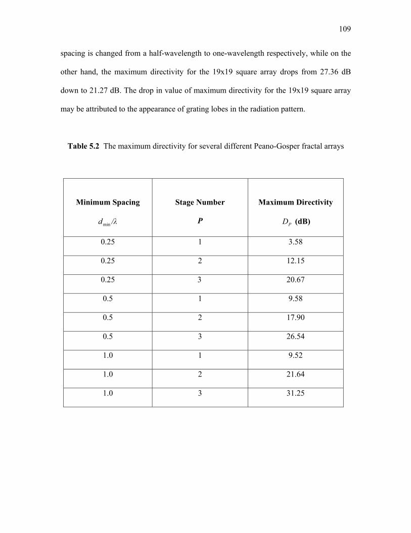
109

spacing is changed from a half-wavelength to one-wavelength respectively, while on the

other hand, the maximum directivity for the 19x19 square array drops from 27.36 dB

down to 21.27 dB. The drop in value of maximum directivity for the 19x19 square array

may be attributed to the appearance of grating lobes in the radiation pattern.

Table 5.2 The maximum directivity for several different Peano-Gosper fractal arrays

Minimum Spacing

/λdmin

Stage Number

P

Maximum Directivity

PD (dB)

0.25 1 3.58

0.25 2 12.15

0.25 3 20.67

0.5 1 9.58

0.5 2 17.90

0.5 3 26.54

1.0 1 9.52

1.0 2 21.64

1.0 3 31.25

110

Table 5.3 Comparison of maximum directivity for a stage 3 Peano-Gosper array with 344 elements and a 19x19 square array with 361 elements


Element Spacing

dmin / λ

Stage 3 Peano-Gosper Array

19x19 Square Array

0.25

20.67 21.42

0.5

26.54 27.36

1.0

31.25 21.27

Next, we consider the case where the mainbeam of the Peano-Gosper fractal array

is steered in the direction corresponding to θ = θo and ϕ = ϕo. In order to accomplish

this, the element phases for the Peano-Gosper fractal array are chosen according to

)cos(sin noonn kr ϕϕθβ −−= (5.30)

Normalized array factor plots with the mainbeam steered to θo = 45° and ϕo = 0° are

shown in Figure 5.15; one for a Stage 3 Peano-Gosper fractal array where the minimum

spacing between elements is a half-wavelength (solid curve) and the other for a

conventional 19x19 uniformly excited square array with half-wavelength element

spacings (dashed curve). This comparison demonstrates that the Peano-Gosper array is

superior to the 19x19 square array in terms of its overall sidelobe characteristics.

111

-80 -60 -40 -20 0 20 40 60 80 -80

-70

-60

-50

-40

-30

-20

-10

0

Theta (degrees)

Arra

y Fa

ctor

(dB)

Figure 5.15 Plots of the normalized array factor versus θ for ϕ = 0° with mainbeam steered to θo = 45° and ϕo = 0°. The solid curve represents the radiation pattern of a stage 3 Peano-Gosper fractal array with 2/min λ=d and the dashed curve represents the radiation pattern of a uniformly excited 19x19 square array with 2/min λ=d

Finally, we note that Peano-Gosper arrays are self-similar since they may be

formed in an iterative fashion so that the array at stage P is composed of seven identical

stage P-1 sub-arrays, i.e., they consist of arrays of arrays. For example, the Stage 2

Peano-Gosper array is composed of seven Stage 1 sub-arrays. Likewise, the Stage 3

Peano-Gosper array consists of seven Stage 2 sub-arrays, and so on. Figure 5.16

illustrates schematically this unique arrangement or tiling of sub-arrays for a Stage 2 and

a Stage 4 Peano-Gosper array.

112

Figure 5.16 Modular architecture of the Peano-Gosper array based on the tiling of Gosper islands. A stage 2 and stage 4 Peano-Gosper array are shown divided up into seven stage 1 and stage 3 Peano-Gosper sub-arrays respectively

This lends itself to a convenient modular architecture whereby each of these sub-arrays

could be individually controlled. In other words, the unique arrangement of tiles forms

sub-arrays that could be designed to support simultaneous multibeam and multifrequency

operation.

Stage 1

Stage 2

Stage 4

113

5.4 Conclusions

A new class of self-similar fractal arrays, called Peano-Gosper fractal arrays, have

been introduced in this chapter. The elements are uniformly distributed along a self-

avoiding Peano-Gosper curve, which results in a deterministic fractal array configuration

composed of a unique arrangement of parallelogram cells bounded by an irregular closed

Koch curve. One of the main advantages of these Peano-Gosper fractal arrays is that they

are relatively broadband compared to conventional periodic planar phased arrays with

regular boundary contours. In other words, they possess no grating lobes even for

minimum element spacings of at least one-wavelength. An efficient iterative procedure

useful for rapidly calculating the radiation patterns of Peano-Gosper fractal arrays to

arbitrary stage of growth P was also presented.

114

Chapter 6

Other Broadband Arrays Produced by Fractal Tilings

6.1 The Terdragon and the 6-Terdragon Arrays

The terdragon is one type of fractal comprised of conjoined triangles tiling a region.

The construction of a terdragon may be described as follows:

1. Start with an initiator (line segment) shown in Figure 6.1(a).

Figure 6.1(a) Initiator for a terdragon curve

2. At stage 1, replace each individual line with the generator which is scaled by a

factor ( )°=30cos2

1s and rotated clockwise by an angle of 30°

Figure 6.1(b) Construction of a stage 1 terdragon curve. The solid curve denotes the generator whereas the dashed curve denotes the initiator

115

3. For further stages, repeat step 2.

Figure 6.1(c) Construction of a stage 2 terdragon curve. The solid curve denotes the generator for the terdragon curve or the stage 2 terdragon curve whereas the dashed curve denotes the stage 1 terdragon curve

Figure 6.2 shows the stage 6 terdragon curve generated by applying the construction

procedure introduced earlier.

Figure 6.2 Stage 6 terdragon curve

116

The 6-terdragon curve may now be constructed by joining together six terdragon

curves around a common central point. The construction of a 6-terdragon curve at stage 1

is illustrated in Figure 6.3. Figure 6.3 shows that the 6-terdragon may be generated by six

terdragons; each of which is rotated by an angle of 2(i-1)π /3, i = 1, 2,....3. The stage 3 6-

terdragon curve is shown in Figure 6.4.

Figure 6.3 The first stage in the construction of a 6-terdragon curve. The initiator is shown as the dashed line superimposed on the stage 1 generator.

Figure 6.4 Stage 3 6-terdragon curve

117

6.1.1 Construction of the Terdragon Fractal Array

A Stage 1, Stage 3, and Stage 6 fractal array based on the terdragon are shown in

Figure 6.5.

1

2

2

1

2

1

2

4

4

4

2

2

6

6

2

2

4

4

4

2

1

2

Stage 1 Stage 3

2

2

2

4

2

6

4

2

4

4

1

2

4

6

6

6

2

2

6

4

4

66

4

4

6

2

2

6

6

6

6

2

2

4

6

4

2

4

6

6

6

6

6

4

2

2

6

6

6

4

2

4

6

6

6

6

6

6

6

6

4

2

4

6

6

6

2

2

4

6

6

6

6

6

6

2

4

2

6

6

4

2

2

6

2

6

6

6

6

6

6

4

2

2

4

6

4

6

2

6

4

4

4

6

6

4

6

2

6

6

6

6

6

6

6

6

6

6

4

6

6

6

6

4

6

6

2

6

6

6

6

6

6

2

6

6

6

6

6

6

6

6

6

2

6

4

6

6

6

6

4

6

2

2

6

4

6

6

6

6

4

6

2

6

6

6

6

6

6

6

6

6

2

6

6

6

6

6

6

2

6

6

4

6

6

6

6

4

6

6

6

6

6

6

6

6

6

6

2

6

4

6

6

4

4

4

6

2

6

4

6

4

2

2

4

6

6

6

6

6

6

2

6

2

2

4

6

6

2

4

2

6

6

6

6

6

6

4

2

2

6

6

6

4

2

4

6

6

6

6

6

6

6

6

4

2

4

6

6

6

2

2

4

6

6

6

6

6

4

2

4

6

4

2

2

6

6

6

6

2

2

6

4

4

66

4

4

6

2

2

6

6

6

4

2

1

4

4

2

4

6

2

4

2

2

2

Figure 6.5 Element locations and associated current distribution for the stage 1, stage 3, and stage 6 terdragon fractal arrays with the minimum spacing between elements and expansion factor denoted by dmin and δ, respectively. The spacing dmin is assumed to be the same for each stage

Stage 6

118

Figure 6.5 also shows the location of the elements and their corresponding current

excitation values. The minimum spacing between array elements is held fixed at a value

of dmin for each stage of growth. The array factor of a stage P terdragon fractal array may

be expressed in terms of P 3x3 matrices which are pre-multiplied by a vector AP and

post-multiplied by a vector C such that

( ) CBA PP=ϕθ ,PAF (6.1)

where

[ ]321 aaa=PA (6.2)

( )( )[ ]αϕϕθ 1cossincos2 min −+−= Pkda ii (6.3)

( )3

21 πϕ −= ii (6.4)

[ ]T001=C (6.5)

∏=

−==P

pP1PpP FBFB

1

(6.6)

[ ]( )33xp

ijf=pF (6.7)

119

[ ]∑∈

+−+−−=ijNn

njnpp

ij pPjkrf ])1(cos[sinexp αγϕϕθ (6.8)

221nn

pnp yxr += −δ (6.9)

<+

=

>

=

0,arctan

0,0

0,arctan

nn

n

n

nn

n

n

xxy

x

xxy

π

γ (6.10)

3,2,1where3

2)1( =−= jjjπϕ (6.11)

°= 30α (6.12)

( )°= 30cos2δ (6.13)

Note that the parameter δ represents the scale factor used to generate the terdragon and

the 6-terdragon fractal arrays. Also, we note that if Nij = φ , then ,0=pijf where the values

of ijN required in (6.8) are found from

[ ]( )

{ } { }{ } { }

{ } { }

==

3,123,12

23,1

33

φφ

φ

xijNN (6.14)

The values of xn and yn required in (6.9) and (6.11) for n = 1-3 are listed in Table 6.1.

120

Table 6.1 Expressions of xn and yn in terms of the parameters dmin, α and δ

n

xn

yn

1 -δdmin/2 -δdmin/4

2 0 0

3 δdmin/2 δdmin/4

6.1.2 Construction of the 6-Terdragon Fractal Array

The first three stages (i.e., P = 1, P = 2, and P = 3) in the construction of a fractal

array based on the 6-terdragon curve are shown in Figure 6.6.

1

1

4

4

1

4

6

4

1

4

4

1

1

1

2

4

2

1

4

4

1

4

6

4

2

6

6

4

6

4

6

6

2

4

6

4

1

4

4

1

2

4

2

1

Stage 1 Stage 2

121

2

1

2

4 4

4

2

2

2

1

2

4

6

6

4

4

4

1

2

4

4

6

6

6

6

6

4

2

4

6

6

6

6

6

6

2

4

6

6

6

6

6

4

2

6

6

6

6

6

6

4

2

4

6

6

6

6

6

4

4

2

1

4

4

4

6

6

4

2

1

2

2

2

4

4

4

2

1

2

Stage 3

Figure 6.6 Element locations and associated current distribution for the stage 1, stage 2 and stage 3 6-terdragon fractal arrays with the minimum spacing between elements and expansion factor denoted by dmin and δ respectively. The spacing dmin is assumed to be the same for each stage Figure 6.6 also shows the location of the elements and their corresponding current

excitation values. The minimum spacing between array elements is held fixed at a value

of dmin for each stage of growth. The array factor of a stage P 6-terdragon fractal array

may be expressed in terms of P 3x3 matrices which are pre-multiplied by a vector AP and

post-multiplied by a vector CP such that

( ) PPP CBA=ϕθ ,PAF (6.15)

[ ]TPPP ccc 3,2,1,=PC (6.16)

122

( )( )iP

iP dkc ϕϕθδ −= − cossincos2 min1

, (6.17)

The matrices AP and BP are defined in (6.2) and (6.6).

6.1.3 Radiation Characteristics of the Terdragon and 6-Terdragon Fractal Arrays

Figure 6.7 Plot of the normalized array factor for the stage 6 terdragon fractal array with minimum spacing dmin = λ in terms of nx and ny

The maximum allowable angle steered from broadside of the stage 6 terdragon

fractal array may be determined from Figure 6.7. By choosing (nx, ny) = (0.95, 0.6) in

Figure 6.7 to be on the boundrary of the visible region, the maximum allowable angle

steered from broadside (θ max) may be obtained using (1.18), ( )1arcsinmax −= bθ , where b

ny

nx

dB

123

is the distance from the origin to the chosen threshold point. The distance b may be

obtained as 1236.16.095.0 22 =+ . Consequently, the maximum allowable angle θ max,

for minimum spacing of dmin = λ, is .09.7 o For minimum spacings dmin = 0.5 λ to λ, the

maximum allowable angle steered from broadside may be obtained by modifying (1.18)

as:

>

−°

≤

−≤

−

=11,90

110,1arcsin

min

minminmax

bd

bd

bd

λ

λλ

θ (6.18)

A plot of maximum allowable angleθ max versus dmin is shown in Figure 6.8.

0.5 0.55 0.6 0.65 0.7 0.75 0.8 0.85 0.9 0.95 10

10

20

30

40

50

60

70

80

90

Minimum Spacing dmin

Max

imum

Allo

wab

le S

teer

ed A

ngle

(deg

rees

)

Figure 6.8 Plot to show maximum allowable angle (θmax) versus minimum spacing between adjacent elements dmin in λ for the stage 6 terdragon fractal array

124

Figure 6.9 Plot of the normalized array factor for the stage 3 6-terdragon fractal array with minimum spacing dmin = λ in terms of nx and ny

The maximum allowable angle steered from broadside for the stage 3 6-terdragon

fractal array may be determined from Figure 6.9. By choosing (nx, ny) = (0.5, 0.9) in

Figure 6.9 to be on the boundary of the visible region, the maximum allowable angle

steered from broadside (θ max) may be obtained from (1.18), ( )1arcsinmax −= bθ , where b

is the distance from the origin to the chosen threshold point. The distance b may be

obtained as 029.19.05.0 22 =+ . Consequently, the maximum allowable angle θ max, for

minimum spacing of dmin = λ, is .66.1 o For minimum spacings dmin = 0.5 λ to λ, the

maximum allowable angle steered from broadside obtained using (6.18) is shown in

Figure 6.10 which contains a plot of the maximum allowable angleθ max versus dmin.

ny

nx

dB

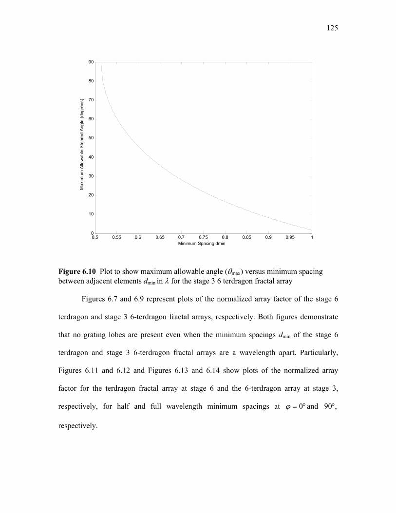
125

Figure 6.10 Plot to show maximum allowable angle (θmax) versus minimum spacing between adjacent elements dmin in λ for the stage 3 6 terdragon fractal array

Figures 6.7 and 6.9 represent plots of the normalized array factor of the stage 6

terdragon and stage 3 6-terdragon fractal arrays, respectively. Both figures demonstrate

that no grating lobes are present even when the minimum spacings dmin of the stage 6

terdragon and stage 3 6-terdragon fractal arrays are a wavelength apart. Particularly,

Figures 6.11 and 6.12 and Figures 6.13 and 6.14 show plots of the normalized array

factor for the terdragon fractal array at stage 6 and the 6-terdragon array at stage 3,

respectively, for half and full wavelength minimum spacings at °= 0ϕ and ,90°

respectively.

0.5 0.55 0.6 0.65 0.7 0.75 0.8 0.85 0.9 0.95 1 0

10

20

30

40

50

60

70

80

90

Minimum Spacing dmin

Max

imum

Allo

wab

le S

teer

ed A

ngle

(deg

rees

)

126

0 10 20 30 40 50 60 70 80 90-80

-70

-60

-50

-40

-30

-20

-10

0

Theta (degrees)

Ar

ray

Fact

or (d

B)

Figure 6.11 Plot of the normalized stage 6 terdragon fractal array factor versus θ with ϕ = 0° for dmin = λ/2 (dashed curve) and dmin = λ (solid curve)

0 10 20 30 40 50 60 70 80 90 -80

-70

-60

-50

-40

-30

-20

-10

0

Theta (degrees)

Arra

y Fa

ctor

(dB)

Figure 6.12 Plot of the normalized stage 6 terdragon fractal array factor versus θ with ϕ = 90° for dmin = λ/2 (dashed curve) and dmin = λ (solid curve)

127

0 10 20 30 40 50 60 70 80 90 -80

-70

-60

-50

-40

-30

-20

-10

0

Theta (degrees)

A

rray

Fac

tor (

dB)

Figure 6.13 Plot of the normalized stage 3 6-terdragon fractal array factor versus θ with ϕ = 0° for dmin = λ/2 (dashed curve) and dmin = λ (solid curve)

0 10 20 30 40 50 60 70 80 90 -80

-70

-60

-50

-40

-30

-20

-10

0

Theta (degrees)

A

rray

Fac

tor (

dB)

Figure 6.14 Plot of the normalized stage 3 6-terdragon fractal array factor versus θ with ϕ = 90° for dmin = λ/2 (dashed curve) and dmin = λ (solid curve)

128

Figure 6.15 and Figure 6.16 show plots of the normalized array factor (in dB) for the

case where dmin = λ and θ = 90° versus azimuth for the stage 6 terdragon and the stage 3

6-terdragon fractal array, respectively. These plots show that no grating lobes are present

anywhere in the azimuthal plane of the stage 6 terdragon and stage 3 6-terdragon fractal

arrays, even with elements spaced one-wavelength apart. In fact, the highest sidelobes in

the azimuthal plane are -19 dB and -16.8 dB, respectively, when the mainbeam is at θ =

0°. For example, the highest sidelobe occurs at ϕ = 97° for th stage 6 terdragon fractal

array when θ = 90° and dmin = λ (Figure 6.15). In the case of the stage 3 6-terdragon

fractal array, the highest sidelobe occurs at ϕ = 11° under the same conditions (see Figure

6.16).

0 50 100 150 200 250 300 350 -80

-70

-60

-50

-40

-30

-20

-10

0

Phi (degrees)

Arr

ay F

acto

r (dB

)

Figure 6.15 Plot of the normalized stage 6 terdragon fractal array factor versus ϕ for θ = 90° and dmin = λ

129

0 50 100 150 200 250 300 350 -80

-70

-60

-50

-40

-30

-20

-10

0

Phi (degrees)

Arra

y Fa

ctor

(dB

)

Figure 6.16 Plot of normalized stage 3 6-terdragon fractal array factor versus ϕ for θ = 90° and dmin = λ

0 10 20 30 40 50 60 70 80 90 -80

-70

-60

-50

-40

-30

-20

-10

0

Theta (degrees)

Arra

y Fa

ctor

(dB

)

Figure 6.17 Plot of the normalized stage 6 terdragon fractal array factor versus θ for ϕ = 97°

130

0 10 20 30 40 50 60 70 80 90 -80

-70

-60

-50

-40

-30

-20

-10

0

Theta (degrees)

Arr

ay F

acto

r (dB

)

Figure 6.18 Plot of the normalized stage 3 6-trdragon fractal array factor versus θ for ϕ = 11°

As in the case of the Peano-Gosper fractal arrays [62], these curves show that for

terdragon and 6-terdragon fractal arrays that no grating lobes appear in the radiation

pattern when the minimum spacing is changed from half-wavelength to at least a full-

wavelength. For comparison purposes, we consider a uniformly excited periodic 18x18

square array of comparable size to the stage 6 terdragon array, which contains a total of

308 elements and a uniformly excited periodic 9x9 square array of comparable size to the

stage 3 6-terdragon fractal array, which contains a total of 79 elements. Plots of the

normalized array factor for the 18x18 square and the 9x9 square array are shown in

Figure 6.19 and Figure 6.20, respectively, for element spacings of dmin = λ/2 (dashed

curve) and dmin = λ (solid curve). A grating lobe is clearly visible for the case in which

the elements are periodically spaced one wavelength apart. The solid curves shown in

Figures 6.21 and 6.22 are plots of the stage 6 terdragon and stage 3 6-terdragon arrays,

131

respectively, for the case where the minimum spacing between elements is increased to

two wavelengths (i.e., dmin = 2λ).

0 10 20 30 40 50 60 70 80 90 -80

-70

-60

-50

-40

-30

-20

-10

0

Theta (degrees)

A

rray

Fac

tor (

dB)

Figure 6.19 Plot of the normalized array factor versus θ at ϕ = 0° for a uniformly excited 18x18 periodic square array with dmin = λ/2 (dashed curve) and dmin = λ (solid curve)

0 10 20 30 40 50 60 70 80 90 -90

-80

-70

-60

-50

-40

-30

-20

-10

0

Theta (degrees)

A

rray

Fac

tor (

dB)

Figure 6.20 Plot of the normalized array factor versus θ with ϕ = 0° for a uniformly excited 9x9 periodic square array with dmin = λ/2 (dashed curve) and dmin = λ (solid curve)

132

For comparison, plots of the array factor for a uniformly excited 18x18 and 9x9 square

array with elements spaced two wavelengths apart have been included in Figure 6.21 and

Figure 6.22, respectively. The two grating lobes that are present in the radiation pattern of

the conventional 18x18 square and 9x9 square arrays are clearly evident in these plots.

The array factor of a stage P terdragon, 6-terdragon, or NxN square array with NP

elements may be expressed in the alternative form:

[ ]∑∑==

+−=•=PP N

nnnnn

N

nnnnP krjInrjkjIAF

11

)cos(sinexp)ˆexp()exp(),( βϕϕθβϕθ r

(6.19)

where nI and nβ represent the excitation current amplitude and phase of the nth

element, nrr is the horizontal position vector of the nth element (with magnitude rn and

phase angle ϕn), and n is the unit vector in the direction of the far-field observation point.

An expression for the maximum directivity of a broadside stage P terdragon, 6-terdragon,

or NxN square array of isotropic sources can be readily obtained by setting 0=nβ in

(6.19) and substituting the result into

∫ ∫= ππ

ϕθθϕθπ

ϕθ2

0 0

2

2

max

sin),(41

),(

ddAF

AFD

P

PP (6.20)

133

0 10 20 30 40 50 60 70 80 90 -80

-70

-60

-50

-40

-30

-20

-10

0

Theta (degrees)

A

rray

Fac

tor (

dB)

Figure 6.21 Plot of the normalized array factor versus θ with ϕ = 0° with dmin = 2λ for the stage 6 terdragon fractal array (solid curve) and a uniformly excited 18x18 square array (dashed curve)

0 10 20 30 40 50 60 70 80 90 -80

-70

-60

-50

-40

-30

-20

-10

0

Theta (degrees)

Arr

ay F

acto

r (dB

)

Figure 6.22 Plot of the normalized array factor versus θ for ϕ = 0° and dmin = 2λ for the stage 3 6-terdragon fractal array (solid curve) and a uniformly excited 18x18 square array (dashed curve)

134

This leads to the following expression for the maximum directivity given by [2]:

( )( )∑∑∑

∑

=

−

==

=

−−

+

=PP

P

N

m

m

n mn

mnmn

N

nn

N

nn

P

rrkrrk

III

ID

2

1

11

2

2

1

sin2 rr

rr (6.21)

Table 6.2 Maximum directivity for several different terdragon fractal arrays

Minimum Spacing

/λdmin

Stage Number

P

Maximum Directivity

PD (dB)

0.25 1 1.5

0.25 3 6.2

0.25 6 19.5

0.5 1 5.7

0.5 3 12.4

0.5 6 25.6

1.0 1 5.6

1.0 3 13.4

1.0 6 29.8

135

Table 6.3 Maximum directivity for several different 6-terdragon fractal arrays.

Minimum Spacing

/λdmin

Stage Number

P

Maximum Directivity

PD (dB)

0.25 1 4.0

0.25 2 8.8

0.25 3 13.4

0.5 1 10.7

0.5 2 15.0

0.5 3 19.4

1.0 1 10.8

1.0 2 17.9

1.0 3 23.8

Tables 6.2 and 6.3 show the maximum directivity values, calculated using (6.21) for the

terdragon and 6-terdragon arrays, respectively, for several different minimum element

spacings dmin and stages of growth P. Tables 6.4 and 6.5 compare maximum directivity

values of a stage 6 terdragon fractal array with those of a conventional uniformly excited

18x18 planar square array, and a comparison between the maximum directivity of a stage

3 6-terdragon fractal array, with those of a conventional uniformly excited 9x9 planar

square array, respectively. These directivity comparisons are made for three different

values of array element spacings (i.e. dmin = λ/4, λ/2, and λ). In the first case, where the

136

element spacing is assumed to be dmin = λ/4, we find that the maximum directivity values

of the stage 6 terdragon array and the 18x18 square array are comparable and so are those

of the stage 3 6-terdragon array and 9x9 square array. This is also true when the element

spacing is increased to dmin = λ/2 (see Table 6.4 and Table 6.5).

Table 6.4 Comparison of maximum directivity of a stage 6 terdragon array of 308 elements with a 18x18 square array of 324 elements

Maximum Directivity (dB) Element Spacing

(dmin/λ) Stage 6 Terdragon Array 18x18 Square Array

0.25 19.48 21.0

0.5 25.6 26.9

1 29.83 20.9

Table 6.5 Comparison of maximum directivity of a stage 3 6-terdragon array of 79 elements with a 9x9 square array of 81 elements


Element Spacing

(dmin/λ) Stage 3 6-Terdragon Array 9x9 Square Array

0.25 13.36 15.0

0.5 19.38 20.7

1 23.75 16.3

137

However, in the third case where the element spacing is increased to dmin = λ, we

see that the maximum directivity values of the stage 6 terdragon fractal array and the

stage 3 6-terdragon fractal array are higher than the corresponding conventional array by

about 9 and 7 dB, respectively. This is because the maximum directivity for the stage 6

terdragon fractal array and the stage 3 6-terdragon array increase from 25.6 to 29.8 and

from 19.4 to 23.8, respectively, when the element spacing is changed from a half to full-

wavelength, while, on the other hand, the maximum directivity value for the 18x18 and

9x9 square arrays drop from 26.9 to 20.9 and from 20.7 to 16.3, respectively. This drop in

the maximum directivity value may be attributed to the appearance of grating lobes in the

radiation pattern.

Next, we consider the case where the mainbeam of the terdragon and the 6-

terdragon fractal arrays are steered in the direction corresponding to θ = θo and ϕ = ϕo. In

order to accomplish this, the element phases for the terdragon and the 6-terdragon fractal

arrays are chosen according to

)cos(sin noonn kr ϕϕθβ −−= (6.22)

Normalized array factor plots with the mainbeam steered to θo = 45° and ϕo= 0° are

shown in Figure 6.23 and Figure 6.24. The solid curves represent plots for the stage 6

terdragon and stage 3 6-terdragon fractal arrays, respectively, and the dashed curves

represent those for the conventional 18x18 and 9x9 uniformly excited square arrays. The

minimum spacing between elements for these cases is a half-wavelength. This

comparison demonstrates that the terdragon and the 6-terdragon fractal arrays are

superior to the 18x18 and 9x9 square arrays, respectively, with diminished overall

sidelobe characteristics.

138

-80 -60 -40 -20 0 20 40 60 80 -80

-70

-60

-50

-40

-30

-20

-10

0

Theta (degrees)

Arra

y Fa

ctor

(dB)

Figure 6.23 Plots of the normalized array factor versus θ for ϕ = 0° and dmin = λ/2 with mainbeam steered to θo = 45° and ϕo = 0°. The solid curve represents the radiation pattern of a stage 6 terdragon fractal array, and the dashed curve represents the radiation pattern of a uniformly excited 18x18 square array

-80 -60 -40 -20 0 20 40 60 80 -80

-70

-60

-50

-40

-30

-20

-10

0

Theta (degrees)

Arra

y Fa

ctor

(dB)

Figure 6.24 Plots of the normalized array factor versus θ for ϕ = 0° and dmin = λ/2 with mainbeam steered to θo = 45° and ϕo = 0°. The solid curve represents the radiation pattern of a stage 3 6-terdragon fractal array, and the dashed curve represents the radiation pattern of a uniformly excited 9x9 square array

139

6.1.4 Conclusions

A new class of self-similar tiled arrays, called terdragon and 6-terdragon fractal

arrays, has been introduced in Section 6.1. Similar to the case of the Peano-Gosper fractal

arrays, the elements of the terdragon and 6-terdragon fractal arrays are uniformly

distributed along terdragon and 6-terdragon curves, respectively, which result in

deterministic array configurations. As is true with the Peano-Gosper fractal arrays, one

of the main advantages of these terdragon and 6-terdragon fractal arrays is that they are

relatively broadband compared to conventional periodic phased arrays. In other words,

they possess no grating lobes even for minimum spacings of at least one-wavelength.

Efficient iterative procedures useful for rapidly calculating the radiation patterns of

terdragon and 6-terdragon fractal arrays to arbitary stage of growth P were also

presented.

140

Chapter 7

Coordinate Transformation for 3-D Antenna Arrays and its Application to Beamforming

Three-dimensional antenna arrays are arrays of antenna elements that occupy

three-dimensional space. These antenna arrays are presumably better as directional

antenna arrays than their planar counterparts since the occupied area projected onto the

plane perpendicular to the mainbeam direction of 3-D antenna arrays is less sensitive to

the variations in mainbeam direction. This chapter introduces coordinate transformations

applicable to direction scanning of 3-D antenna arrays. This is used for beamforming of

the 3-D fractal antenna arrays introduced in the next chapter.

Consider an N-element antenna array located in three-dimensional space. Suppose

that the nth element of the 3-D array is located at the rectangular coordinate (xn, yn, zn)

shown in Figure 7.1 with the position vector nrr . Suppose that the nth element of the array

has current amplitude excitation In and relative phase βn. In terms of the position

vector nrr , the array factor of this 3-D antenna array can be expressed as:

∑=

+•=N

nnnn nrkjInAF

1

)]ˆ([exp)ˆ( βr (7.1)

where n is a unit vector in the direction of the field point.

141

θ

ϕ

the rectangular coordinates (xn,yn,zn) or the cylindrical coordinates ( )nnn z,,ϕρ

x

y

z

mainbeam direction ϕ = ϕo and θ = θo

and unit direction vector 'z

the nth element

z′

unit direction vector x′ in direction of θ = θo+π and ϕ = -ϕo

a plane perpendicular to the mainbeam direction

x′

y′

nr

r

nρ

Figure 7.1 Rectangular coordinates (xn,yn,zn) and cylindrical coordinates ( )nnn z,,ϕρ and projection plane in the direction of ϕ = ϕo and θ = θo

142

The expression for the array factor in terms of rectangular coordinates (xn, yn, zn)

is very complicated. Therefore, in order to avoid this complexity, we transform the

expression from the rectangular coordinates ( )nnn zyx ,, to the cylindrical coordinates

)( n nn z,, ′′′ ϕρ . This can be performed in two steps. First, we transform the coordinate

(xn,yn,zn) to the coordinate )( nnn z,y,x ′′′ by using a transformation T determined by (7.2),

=

′′′

n

n

n

n

n

n

zyx

Tzyx

(7.2)

The transformation T may be represented using two matrices associated with rotation and

translation. In other words, the transformation T may be represented using matrices Tr

and Tt. Hence, the expression in (7.2) may be represented in matrix form as:

tr TT +

=

′′′

n

n

n

n

n

n

zyx

zyx

(7.3)

The matrix Tr may be found by the relation between the unit vectors x , y and z

associated with the rectangular coordinates ),,( nnn zyx and the unit vectors x′ˆ , y′ˆ and

z′ˆ associated with the coordinates ),,( nnn zyx ′′′ , where the unit vector z′ˆ is in the

mainbeam direction and the unit vectors x′ˆ and y′ˆ are orthogonal to each other and

aligned on a plane perpendicular to the mainbeam direction. The unit vector x′ˆ may be

143

selected to be a unit vector in the direction of θ = θo+π/2 and ϕ = ϕo. By the right hand

rule, the unit vector y′ˆ may be defined as x zy ′×′=′ ˆˆˆ . Hence, yx ′′ ˆ,ˆ and z′ˆ may be

expressed as:

−=

′′′

zyx

zyx

ˆˆˆ

cossinsincossin0cossin

sin-sincoscoscos

ˆˆˆ

ooooo

oo

ooooo

θϕθϕθϕϕ

θϕθϕθ (7.4)

This implies that the matrix Tr corresponding to (7.4) is:

−=

ooooo

oo

ooooo

cossinsincossin0cossin-

sinsincoscoscos

θϕθϕθϕϕ

θϕθϕθ

rΤ (7.5)

and the matrix Tt may be expressed as:

−=

c00000000

tT (7.6)

The constant c in (7.6) is arbitrary. For simplicity, the constant c is selected so that max

{zn}= 0. Therefore, the coordinates ),,( nnn zyx ′′′ may be expressed as (7.7)

144

−+

−=+

=

′′′

czyx

zyx

zyx

n

n

n

n

n

n

n

n

n

00000000

cossinsincossin0cossin-

sinsincoscoscos

ooooo

oo

ooooo

θϕθϕθϕϕ

θϕθϕθ

tr TT (7.7)

The next step is to transform the rectangular coordinates )z,,( nnn yx ′′′ to the

coordinates ),( nnn z, ′′′ ϕρ shown in Figure 7.2.

y′

z '

θ ′

ϕ′

( )nnn z′′′ ,,ϕρ

The plane perpendicular to the direction ϕ =ϕo and θ = θo or the unit direction vector z′ˆ in Fig. 7.1

x′

nr ′

Figure 7.2 Projection plane and the cylindrical coordinate system

145

The array factor in (7.1) can be rewritten as:

∑=

′++′−′′′=′′N

nnnnnn zkθkjI,θAF

1)])(cossin([exp)( βϕϕρϕ (7.8)

The mainbeam can be steered to the direction of θ = θo and ϕ = ϕo or in the direction of

the z′ -axis shown in Figures 7.1 and 7.2, by setting the phase term of (7.8) to be in phase

in the direction of 0θ =′ . This leads to the equation

0constant ==′+ nn zkβ . (7.9)

Hence, the phase βn can be expressed as:

'zcf'kz nnn πβ 2−=−= (7.10)

The phase βn is obviously proportional to the frequency f. It should be noted that the

array factor of the planar array whose mainbeam is steered to the direction of θ = θo and

ϕ =ϕo can be expressed as:

])cos()sin([e),( nN

1n

nnn

θkjIθAF βϕϕρϕ +−= ∑=

(7.11)

where

( ) ( )nnn k ϕϕθρβ −−= oo cossin , (7.12)

k = 2π/λ (the wave number in free space)

146

nρ and ϕn are the associated polar coordinates of the nth element and

In is the relative current amplitude excitation of the nth element

may be derived using the principle introduced earlier, i.e., by setting the constant c = 0 in

(7.7), we find that the planar arrays discussed in previous sections can be treated as a

particular case of 3-D arrays. Obviously, by inspection, 'zn may be expressed as:

( ) ( )noonnz ϕϕθρ −=′ cossin (7.13)

Therefore, by applying (7.10), the phase βn of the nth element in (7.12) may be easily

derived.

147

Chapter 8

3-D Fractal Arrays Using Concentric Sphere Array Generators

8.1 Introduction

Three-dimensional volumetric fractal arrays have elements that are located in

three dimensional space. Their structures exhibit a property known as “self-similarity”.

Different from that of the 2-D (planar) arrays, the area projected to the plane

perpendicular to the mainbeam direction of the 3-D arrays is not significantly dependent

on the mainbeam direction. Hence, 3-D fractal arrays would supposedly perform better as

directional arrays than 2-D fractal arrays. For simplicity, in this chapter, only fractal

arrays generated using a concentric sphere array generator are investigated. Unlike fractal

planar antenna arrays, 3-D fractal arrays frequently contain more than one element in the

mainbeam direction. In practice, real elements always exert mutual coupling on each

other. However, the analysis and synthesis performed in this chapter neglects all mutual

effects between elements since these effects depend upon individual element geometries.

This chapter will focus on the synthesis of Menger sponge and 3-D Sierpinski gasket

arrays. Analysis of these arrays is discussed only briefly since the analysis of 3-D arrays

is much more complicated than that of 2-D arrays.

148

8.2 Synthesis of 3-D Fractal Arrays Using Concentric Sphere Array Generators

The synthesis of 3-D fractal arrays is more complicated than the synthesis of 2-D

fractal arrays. For simplicity, only 3-D fractal arrays using concentric sphere subarrays

are discussed in this chapter. The array factor of a 3-D fractal array generated using

sphere subarray generators may be expressed as:

,)()(1

11∏

=

− Ψ=ΨP

p

pP AFAF

rrδ (8.1)

where

( ) ( ) ( )[ ]kjik ˆcosˆsinsinˆcossin θϕθϕθ ++=Ψr

(8.2)

and ),(1 Ψr

AF the array factor of the generator (stage 1) in (8.1), is given by

])(cossin[exp),(),(1

1 nnnn

N

nn jkzjθjkIAFAF ++−== ∑

=

βϕϕρϕθϕθ (8.3)

As described in Chapter 7, the array factor ( )ϕθ,1AF may be expressed in the coordinates

),( ϕθ ′′ using (7.8):

( ) ∑=

′++′−′′′=′′=N

nnnnnn zkθkjI,θAFAF

111 )])(cossin([exp)(, βϕϕρϕϕθ (8.4)

The mainbeam can be steered to the direction of the axisz′+ by controlling the phase in

the appropriate way. The phase may be expressed as:

149

.'kznn −=β (8.5)

The procedure for synthesizing these fractal arrays is outlined below:

a. Define an initiator and subarray generator of the specific 3-D fractal antenna array. Specify the current excitation of each individual element and the mainbeam direction shown in Figure 7.1.

b. Each individual element may be located in the cylindrical coordinate

system ( )z′′′ ,,ϕρ . Noting that the mainbeam direction coincides with the z′ -direction shown in Figure 7.1 and Figure 7.2 in the previous chapter. The transformation from the rectangular coordinates ( )zyx ,, to the cylindrical coordinates ( )z′′′ ,,ϕρ is introduced in Chapter 7. The phase of each individual element of the subarray generator may be calculated from (8.5).

c. Generate 3-D fractal arrays using the procedure described below.

The 3-D fractal arrays may be generated by an operation, similar to the operation

to generate the 2-D fractal arrays described in Chapter 1. The construction process for a

fractal array begins by starting with an element (initiator) as shown in Figure 8.1.

Figure 8.1 Fractal spherical array initiator (stage 0)

150

Stage 1: Surround the antenna with m concentric spheres of radius rm, and substitute the initiator antenna shown in Figure 8.1 with a generator as shown in Figure 8.2.

Figure 8.2 Fractal spherical array (stage 1)

Stage 2: Expand the size of the array by a factor of δ shown in Figure 8.2 Reiterate the operation performed in stage 1.

Stage P (P > 2): Repeat all further stages similar to the operation performed in stage 2.

By (8.1), the recurrence relation for the array factor can be expressed as:

)()()( 11 ΨΨ=Ψ − AFAFAF PP δ (8.6)

By this recurrence relation, the current amplitude and phase excitation of each individual

generated element are consistent with (8.1), each of which may be expressed as:

11m

Pn

Pn III ′

−′= (8.7)

rm

151

and

11m

Pn

Pn ′

−′ += βδββ (8.8)

where PnI and P

nβ are the current amplitude excitation and phase of the nth element at

stage P generated from the ( )thn′ element at stage P-1 by using the ( )thm′ element of the

subarray generator, respectively, where

( ) mnNn g ′+′= ; Ng is the number of elements of the subarray generator.

1−′

PnI and 1−

′Pnβ are the current amplitude excitation and phase of the

( )thn′ generating element at stage P-1, respectively.

1mI ′ and 1

m′β are the current amplitude excitation and phase of the ( )thm′ element of the subarray generator, respectively.

Consequently, the iterative equation given in (8.8) can be used to derive (7.10) for fractal

arrays that use a spherical subarray generator. This can be interpreted as meaning that the

mainbeam direction of the fractal array is the same as that of the spherical subarray

generator. Also,

we note that the phase βn of the nth element may be computed using the expression:

.'kznn −=β (8.9)

8.2.1 Menger Sponge (3-D Sierpinski Carpet) Array

Menger sponge (also called 3-D Sierpinski carpet) arrays are a special type of

antenna array that occupies 3-D spaces. Their structure is defined to be consistent with

152

the Menger sponge fractal. Menger sponge (3-D Sierpinski carpet) arrays may be

generated using the subarray shown in Figure 8.3. Each individual element is represented

by a cube where the associated element is located at its center. The subarray generator

may be conveniently represented in the form shown in Figure 8.3.

Figure 8.3 Menger sponge subarray generator, where each individual element is represented by a cube Figure 8.4 indicates the location of each individual element denoted by an “x”. The

coordinates for each of these elements are (-dmin, dmin , dmin), (0, dmin, dmin), (dmin, dmin,

dmin), (-dmin,0, dmin), (dmin,0, dmin), (-dmin,- dmin, dmin), (0,- dmin, dmin),( dmin,- dmin, dmin), (-

dmin, dmin,0), (dmin, dmin,0), (-dmin,- dmin,0),( dmin,- dmin,0), (-dmin, dmin,- dmin), (0, dmin,- dmin),

(dmin, dmin,- dmin), (-dmin,0, dmin), (dmin,0,- dmin),(- dmin,- dmin,- dmin), (0,- dmin,- dmin) and

(dmin,- dmin,- dmin).

153

2dmin

2dmin

2dmin

Figure 8.4 Subarray generator of Menger sponge arrays where each individual element is denoted by an “• ”. The minimum spacing between elements is dmin

By choosing δ = 3, the stage 2 Menger sponge (3-D Sierpinski carpet) array is

shown in Figure 8.5, where each individual element is located at the center of a cube.

Figure 8.6 shows the top view of the stage 2 Menger sponge array whereas Figure 8.7

shows the front view of the stage 2 Menger sponge array. Figure 8.8 shows an auxiliary

view of the stage 2 Menger sponge array in the zx ′−′ plane, where the −′z axis is

oriented in the direction of °== 45oθθ and °== 0oϕϕ . The associated array factor

( )ϕθ ,AF may be determined from (8.4). The relative current amplitude excitation In are

uniform (In =1, for all n) but the relative phase βn may be determined by (8.5), such

that 'kznn −=β as shown in Figure 8.8.

154

Figure 8.5 Stage 2 Menger sponge (3-D Sierpinski carpet) array where an individual element is located at the center of each cube

-5 -4 -3 -2 -1 0 1 2 3 4 5-4

-3

-2

-1

0

1

2

3

4

X axis

Y a

xis

Figure 8.6 Top view of the stage 2 Menger sponge array in terms of minimum interelement spacing dmin.

155

-5 -4 -3 -2 -1 0 1 2 3 4 5-4

-3

-2

-1

0

1

2

3

4

X axis

Z ax

is

Figure 8.7 Front view of the stage 2 Menger sponge array, in terms of minimum interelement spacing dmin

-6 -4 -2 0 2 4 6-11

-10

-9

-8

-7

-6

-5

-4

-3

-2

-1

0

X prime axis

Z pr

ime

axis

Figure 8.8 Auxiliary view of the stage 2 Menger sponge array, in terms of interelement spacing dmin. The z′ -axis is oriented to the direction of °= 45θ and °= 0ϕ . The scale is expressed in terms of dmin

156

8.2.1.1 Radiation Characteristics of Menger Sponge Arrays

Figure 8.9 and Figure 8.10 shows plots of the normalized array factor in dB scale

for the stage 2 Menger sponge array with minimum spacing of dmin = λ, where the

mainbeam is steered to the direction of °== 0oθθ and °== 0oϕϕ .

Figure 8.9 Plot of the normalized array factor for the stage 2 Menger sponge array with minimum spacing of dmin = λ where the mainbeam is steered to the direction of

°== 0oθθ and °== 0oϕϕ

ny

nx

dB

157

0 10 20 30 40 50 60 70 80 90-80

-70

-60

-50

-40

-30

-20

-10

0

Theta (degrees)

Nor

mal

ized

Arr

ay F

acto

r (dB

)

Figure 8.10 Plot of the normalized array factor sliced at ϕ = 0º for the stage 2 Menger sponge array with minimum spacing of dmin = λ where the mainbeam is steered to the direction of °== 0oθθ and °== 0oϕϕ

Figure 8.9 shows that, with minimum spacing one wavelength apart, grating lobes are

present in the radiation pattern represented by the visible region (unit circle centered at

the origin (nx,ny) = (0,0)). In particular, the normalized array factor versus θ sliced at ϕ =

0° is illustrated in Figure 8.10 which demonstrates that there is one grating lobe present

in this particular cut (the other grating lobe is not shown in Figure 8.10).

Figure 8.11 and Figure 8.12 show the case where mainbeam is steered to the

direction of °== 45oθθ and °== 0oϕϕ with minimum element spacing of one

wavelength. Figure 8.11 shows that there are large sidelobes present in the radiation

158

pattern represented by the visible region (unit circle centered at the origin, (nx,ny) = (0,0)).

As shown in Figure 8.12, the normalized array factor versus θ sliced at ϕ = 0° indicates a

relatively high sidelobe level compared to the overall radiation pattern.


°== 45oθθ and °== 0oϕϕ . The horizontal and vertical axes are denoted by xn and yn ,

respectively, where 1222 =++ zyx nnn

nx

ny

dB

159


°== 45oθθ and °== 0oϕϕ

8.2.2 3-D Sierpinski Gasket Arrays

3-D Sierpinski gasket arrays are 3-D antenna arrays whose structures are

associated with a 3-D version of the Sierpinski gasket. Their subarray generators contain

4 elements. Each of which is located at a vertex of a tetrahedron. The rectangular

coordinates of the nth element ( )nnn zyx ,, are given by [65]

( )minmin 612/1,0,33/1 dd − , ( )minmin 612/1,2/,36/1 dd −±− , and ( )min64/1,0,0 d .

Figure 8.13 shows the stage 1 3-D Sierpinski gasket which contain 4 tetrahedrons; each

of which represents an individual element of the subarray generator. Each individual

element of the subarray generator is denoted by an “x” in Figure 8.14.

-80 -60 -40 -20 0 20 40 60 80-80

-70

-60

-50

-40

-30

-20

-10

0

Theta (degrees)

Nor

mal

ized

Arr

ay F

acto

r (dB

)

160

Figure 8.13 Stage 1 of the 3-D Sierpinski gasket contains 4 tetrahedrons; each of which represents an individual element located at its center

Figure 8.14 Subarray generator of the Sierpinski gasket array

dmindmin

161

The minimum spacing dmin between elements shown in Figure 8.14 may be

determined from the geometry shown in Figure 8.5 [63]. The resulting expression is

found to be

64

minrd = (8.10)

(a) Bottom View (b) Side View

Figure 8.15 Determining minimum spacing dmin of the subarray generators [63]

By choosing the expansion ratio δ = 2, the stage 3 3-D Sierpinski gasket array

may be represented by the stage 3 Sierpinski gasket in Figure 8.16 where each

tetrahedron represents an array element. In other words, each individual element is

located at the centroid of the associated tetrahedron.

r

r

dmin

r

r

dmin/2

162

Figure 8.16 Stage 3 3-D Sierpinski gasket.

Figure 8.17 represents the top view of the stage 3 3-D Sierpinski gasket array

which contains 64 elements. Each individual element is denoted by an “x”. The

horizontal and vertical axes represent the x- and y- axes, respectively. Figure 8.18 shows

the front view of the stage 3 3-D Serpinski gasket array. Also, each individual element is

denoted by an“x”. The horizontal and vertical axes represent the x- and z- axes,

respectively, whereas Figure 8.19 represents an auxiliary view of the stage 3 3-D

Sierpinski gasket array where the horizontal and vertical axes denote the x′ - and z′ -

axes, respectively. The associated array factor ( )ϕθ ,AF may be determined by (8.4). The

relative current excitation In are uniform (In = 1, for all n) but the relative phase βn may

be determined by (8.5), 'kznn −=β as shown in Figure 8.19.

163

-3 -2 -1 0 1 2 3 4 5

-3

-2

-1

0

1

2

3

X axis

Y a

xis

Figure 8.17 Top view of the stage 3 3-D Sierpinski gasket array, scaled in terms of minimum interelement spacing dmin

-2 -1 0 1 2 3 4

-1

-0.5

0

0.5

1

1.5

2

2.5

3

3.5

4

X axis

Z ax

is

Figure 8.18 Front view of the stage 3 3-D Sierpinski gasket array, scaled in terms of minimum interelement spacing dmin

164

-3 -2 -1 0 1 2 3

-5

-4.5

-4

-3.5

-3

-2.5

-2

-1.5

-1

-0.5

0

X prime axis

Z pr

ime

axis

Figure 8.19 Auxiliary view of the stage 3 3-D Sierpinski gasket array, in terms of minimum interelement spacing dmin. The z′ -axis is oriented in the direction of °= 45θ and °= 0ϕ

8.2.2.1 Results of the Stage 3 3-D Sierpinski Gasket Array

Figure 8.20 and Figure 8.21 show plots of the normalized array factor of the stage

3 3-D Sierpinski gasket array with minimum spacing of dmin = λ where the mainbeam is

steered to the direction of °= 0θ and °= 0ϕ ; Figure 8.20 shows a plot of the normalized

array factor in terms of nx and ny where nz is assumed to be nonnegative, as well as Figure

8.21 shows a plot of array factor sliced at a specific angle ϕ = 0°. Figure 8.20 shows that

there are relatively large sidelobes present in the radiation pattern represented by the unit

circle centered at the origin, (nx,ny) = (0,0).

165

Figure 8.20 Plot of the normalized array factor for the stage 3 3-D Sierpinski gasket array with minimum spacing of dmin = λ/2 where the mainbeam is steered to the direction of °== 0oθθ and °== 0oϕϕ . The horizontal and vertical axes denote xn and yn ,


nx

ny dB

166

Figure 8.22 and Figure 8.23 show plots of the normalized array factor of the stage 3 3-D

Sierpinski gasket array with minimum spacing of dmin = λ where mainbeam is steered to

the direction of °= 45θ and °= 0ϕ . Figure 8.22 shows a plot of the normalized array

factor in terms of nx and ny where nz is assumed to be nonnegative, as well as Figure 8.23

shows a plot of the normalized array factor versus θ sliced at a specific angle ϕ = 0°.

Figure 8.22 demonstrates that the overall sidelobe level is still high. This is an

undesirable characteristic for broadband applications.

0 10 20 30 40 50 60 70 80 90-80

-70

-60

-50

-40

-30

-20

-10

0

Theta (degrees)

Nor

mal

ized

Arr

ay F

acto

r (dB

)

Figure 8.21 Plot of the normalized array factor sliced at ϕ = 0º for the stage 3 3-D Sierpinski gasket array with minimum spacing of dmin = λ/2 where the mainbeam is steered to the direction of °== 0oθθ and °== 0oϕϕ

167

Figure 8.22 Plot of the normalized array factor of the stage 3 3-D Sierpinski gasket array with minimum spacing of dmin = λ/2 where mainbeam is steered to the direction of

°== 45oθθ and °== 0oϕϕ . The horizontal and vertical axes are denoted by xn and yn ,


Although the 3-D fractal arrays investigated so far are undesirable to broadband

applications, the half-power beamwidth of the 3-D fractal arrays do not significantly

depend on the steered angle of the mainbeam. This charateristic is different from that of

the 2-D fractal arrays. The 3-D fractal arrays with more complicated structures, e.g., 3-D

Peano-Gosper fractal arrays, could be suitable candidates for broadband directional

arrays.

nx

ny

dB

168

Figure 8.23 Plot of the normalized array factor sliced at ϕ = 0° of the stage 3 3-D Sierpinski gasket array with minimum spacing of dmin = λ where the mainbeam is steered to the direction of °== 45oθθ and °== 0oϕϕ 8.3 Conclusions

While most of the results obtained so far for 3-D arrays are undesirable for

broadband applications, it is observed that the half-power beamwidth of these 3-D fractal

arrays do not significantly depend on the steered angle of the mainbeam. Hence, more

complex-structured 3-D fractal arrays may potentially perform well in antenna

applications requiring high directivity, rapid computations, minimal sidelobe emissions,

and adaptive beamforming.

-80 -60 -40 -20 0 20 40 60 80 -80

-70

-60

-50

-40

-30

-20

-10

0

Theta (degrees)

Nor

mal

ized

Arr

ay F

acto

r (dB

)

169

Chapter 9

Conclusions and Future Work

9.1 Conclusions

The potential benefits of fractal arrays include their multiband/broadband

performance, the ability to exploit the recursive nature of fractals to develop rapid

beamforming algorithms, and the ability to develop schemes for low sidelobe designs.

Moreover, systematic approaches to thinning and efficient design strategies for large 2-D

arrays are possible. Also, it has been shown that they require a minimal amount of

switching when implemented as reconfigurable apertures. The research in this thesis has

led to a new design methodology for modular broadband arrays that is based on the

theory of fractal tilings. This type of fractal array differs fundamentally from other types

of fractal arrays considered in the past that have regular boundaries with elements

distributed in a fractal pattern on the interior. Examples of broadband array

configurations based on fractal tilings developed and studied in this thesis include Peano-

Gosper, Terdragon, and 6-Terdragon arrays.

Several new self-scalable arrays have also been introduced in this thesis,

including pentagonal, octagonal, and honeycomb arrays. These arrays were shown to

possess relatively low-sidelobe characteristics with the added advantage that they can be

generated recursively. This allows for the development of rapid beamforming algorithms

for these arrays. Finally, some preliminarily investigations into the radiation

characteristics of two different 3-D fractal arrays have also been presented. These studies

indicate that the beamwidth of 3-D fractal arrays are less sensitive to the mainbeam scan

direction than their 2-D counterparts.

170

Chapter 1 includes a literature review of fractals and their applications in

electromagnetics. Moreover, Chapter 1 also introduces a family of fractal arrays that are

generated using concentric ring subarrays. Specific examples considered in Chapter 1

include Sierpinski gasket arrays and self-scalable hexagonal arrays. These arrays have

the advantage that they can be recursively generated via a compact product representation

for their array factors.

Chapter 2 further investigates other configurations of fractal arrays that can be

constructed using ring subarray generators. These include self-scalable pentagonal, self-

scalable octagonal, and honeycomb arrays. For both self-scalable pentagonal and self-

scalable octagonal arrays where the minimum element spacing is a half-wavelength, it

was found that the overall sidelobe level can be made lower by inserting an element at the

center of the associated subarray generators. Although, for the case of self-scalable

octagonal arrays, the corresponding beamwidth increases by inserting an element at the

center of the generator, the maximum directivity is seen to increase for minimum element

spacings of both a half wavelength as well as a wavelength.

Chapter 3 reviews briefly the conventional principle of pattern multiplication and

introduces the generalized principle of pattern multiplication. The conventional principle

of pattern multiplication is based on the assumption that the generators for all the

individual elements are the same in their structure, size, and orientation. To eliminate this

assumption, the generalized principle of pattern multiplication is introduced. In this case,

the array factor can be expressed in terms of a summation of all the entries in a particular

matrix representation. This matrix has the property that it can be expressed in terms of the

product of other matrices; each of which represents the array factor for a previously

171

generated subarray. This generalized principle of pattern multiplication is applied in

Chapters 4, 5 and 6 where fractal configurations are formed by generators which are

identical in shape and size but different in orientation.

Chapter 4 introduced the Peano fractal array and the Sierpinski dragon fractal

array. The Peano and Sierpinski dragon fractal arrays do not perform well as broadband

arrays. However, their structures are relatively simple and lead to a better understanding

of the more complicated array configurations introduced later in Chapters 5 and 6.

Chapters 5 and 6 discuss a new class of modular broadband arrays that are based

on applications of tiling theory. These arrays were found to be relatively broadband when

compared to conventional periodic planar arrays that have square or rectangular cells and

regular boundary contours. The analysis presented in Chapter 5 focuses on a specific type

of tiled array called the Peano-Gosper array. Its structure corresponds to the self-avoiding

Peano-Gosper curve. Chapter 6 introduces the terdragon and related 6-terdragon arrays.

Elements of the Peano-Gosper, terdragon and 6-terdragon fractal arrays are distributed

uniformly along a self-avoiding space-filling curve. These arrays are also shown to

belong to the class of deterministic arrays that are almost uniformly excited. For all of

these arrays, it is shown that grating lobes do not appear in their radiation patterns even

when the minimum spacing between elements is increased up to a wavelength. Hence,

these arrays all exhibit broadband operating characteristics. Moreover, both Peano-

Gosper arrays and 6-Terdragon arrays can be partitioned into several identical subarrays;

each of which also represents a broadband array. Hence they can be used for applications

where simultaneous multibeam and multifrequency operation is required.

172

Chapter 7 introduces a convenient coordinate transformation which is used for

beamforming of the 3-D fractal arrays considered in Chapter 8. Chapter 8 presents the

results of a preliminary investigation of the radiation characteristics of 3-D fractal arrays

constructed from concentric sphere generators. Specific configurations considered

include the 3-D Sierpinski carpet (also known as the Menger sponge) and 3-D Sierpinski

gasket arrays. The beamwidth of these 3-D fractal arrays are shown to be less sensitive to

the mainbeam direction than in the case of their 2-D fractal array counterparts.

9.2 Future Work

There are several possible areas that can be explored as future work which build

upon the research presented in this thesis. These include:

• Develop and evaluate the performance of more sophisticated self-scalable array

designs based on concentric ring subarray generators.

• Investigate the radiation characteristics of other array configurations with

irregular boundary contours based on fractal tilings.

• Investigate the relationship between the fractal dimension of the irregular

boundary contour and the corresponding bandwidth of arrays formed via fractal

tilings.

• Develop design approaches for fractal arrays conformal to the surface of curved

objects such as cylindrical and spherical platforms.

• Expand on the preliminary analysis presented in this thesis for generating 3-D

volumetric fractal arrays.

173

• Develop effective beamforming and sidelobe suppression techniques for 3-D

volumetric fractal arrays.

174

References

[1] B. B Mandelbrot, The Fractal Geometry of Nature, New York: W.H. Freeman and

Company, 1977. [2] J. Feder, Fractals, Plenum Press, New York, 1988.

[3] R. L. Haupt, and D. H. Werner, “ Fractal Constructions of Linear and Planar Arrays,” Antennas and Propagation Society International Symposium, Vol. 3, pp. 1968-1971,

1997. [4] C. P. Baliarda, and R. Pous, “Fractal Design of Multi-band and Low Side-Lobe

Arrays,” IEEE Trans. Antennas Propagat., Vol. 44, pp. 730-739, May 1996. [5] D. J. Jaggard, “Prolog Section on Fractals in Electrical Engineering,” Proc. IEEE,

Vol. 81, pp.1423-1427, October 1993. [6] H., -O. Peitgen and D. Saupe, Chaos and Fractals New Frontiers of Science, New

York: Springer-Verlag, 1992. [7] D. H. Werner and P. L. Werner, “Frequency-Independent Features of Self-Similar Fractal Antennas,” Radio Science, Vol. 31, pp.1331-1343, November-December 1996. [8] D. H. Werner and P. L. Werner, “On the Synthesis of Fractal Radiation Patterns,”

adio Science, Vol. 30, pp. 24-45, January – February 1995. [9] D.L Jaggard, On Fractal Electrodynamics, in Recent Advances in Electromagnetic

Theory, H. N. Kritikos and D. L. Jaggard, Eds., New York, Springer- Verlag, 1990. [10] J. L. Vehel, E. Lutton, and C. Tricot, Fractals in Engineering from Theory to

Industrial Applications, Springer Verlag, 1997. [11] M.V. Berry, “Diffractals,” J. Phys. A: Math. Gen., Vol. 12, pp. 781-797, 1979.

[12] M.V. Berry and T.M. Blackwell, “Diffractal Echoes,” J. Phys. A: Math. Gen., Vol.14, pp. 3101-3110, 1981.

[13] E. Jakeman, “Scattering by a Corrugated Random Surface with Fractal Slope,” J.

Phys. A, Vol. 15, L55-L59, 1982. [14] E. Jakeman, “Fresnel Scattering by a Corrugated Random Surface with Fractal

Slope,” J. Opt. Soc. Am., Vol. 72, pp.1034-1041, 1982.

175

[15] E. Jakeman, “ Fraunhofer Scattering by a Sub-Fractal Diffuser,” Optica Acta, Vol. 30, pp. 1207-1212, 1983.

[16] E. Jakeman, “Scattering by Fractals,” in Fractals in Physics, L. Pietronero ans E.

Tosatti, eds., Elsevier Science Publishers B.V. New York, pp.55-60, 1986. [17] C. Allain and M. Cloitre, “Optical Fourier Transforms of Fractals,” in Fractals in

Physics, L. Pietronero and Tosatti, eds, Elsevier Science Publishers B.V., New York, pp.61-64, 1986.

[18] C. Allain and M. Cloitre, “Optical Diffraction on Fractals,” Phys. Rev. B, Vol.33,

3566-3569, 1986. [19] C. Bourrely, P. Chiappetta, and B. Torresani, “Light Scattering by Particles of

Arbitrarily Shape: A Fractal Approach,” J. Opt. Soc. Am. A, Vol. 3, pp. 250-255, 1986.

[20] C. Bourrely and B. Torresani, “Scattering of an Electromagnetic Wave by an

Irregularly Shaped Opject,” Optics Comm., Vol. 58, pp. 365-368, 1986. [21] C. Allain and M. Cloitre, “Spatial Spectrum of a General Family of Self-Similar

Arrays,” Phys. Rev. A, Vol. 36, pp. 5751-5757, 1987. [22] D. L. Jaggard and X. Sun, “Scattering from Bandlimited Fractal Fibers,” IEEE.

Trans. Ant. and Propagat., Vol. 37, pp.1591-1597, 1989.

[23] M.M. Beal and N. George, “Features in the Optical Transforms of Serrated Apertures and Disks,” J. Opt. Soc. Am. A, Vol. 6, pp.1815-1826, 1989.

[24] X. Sun and D. L. Jaggard, “Scattering from Fractally Fluted Cylinders,” J.

Electromagnetic Wave Appl., Vol. 4, pp.599-611, 1990. [25] Y. Kim, H. Grebel, and D. L. Jaggard, “Diffraction by Fractally Serrated Apertures,”

J. Opt. Soc. A, Vol. 8, pp.20-26, 1991. [26] D. L. Jaggard, T. Spielman, and X. Sun, “Diffraction by Cantor Targets,” in

Conference Proceedings of the 1991 AP-S/URSI Meeting, London, Ontario, 1991.

[27] T. Spielman and D. L. Jaggard, “Diffraction by Cantor Targets: Theory and Experiment,” in Conference Proceedings of the 1992 AP-S/URSI Meeting, Chicago, Illinois, 1992.

[28] N. Cohen, “Fractal Antennas: Part 1,” Communications Quarterly, pp.7-22, Summer

1995.

176

[29] N. Cohen, R. G. Hohlfeld, “Fractal Loops and The Small Loop Approximation,” Communications Quarterly, pp. 77-81, Winter 1996.

[30] N. Cohen, “Fractal and Shaped Dipoles,” Communications Quarterly, pp.25-36, Spring 1996.

[31] N. Cohen, “Fractal Antennas: Part 2,” Communications Quarterly, pp.53-66,

Summer 1996. [32] C. Puente, “Fractal Antennas,” Ph.D. Dissertation at the Dept. of Signal Theory and

Communications Letters, Universitat Politecnica de Catalunya (UPC), June 1997. [33] C. Puente, J. Romeu, R. Pous, J. Ramis, and A. Hijazo, “Small but long Koch fractal

monopole,” IEE Electronics Letters, Vol. 34(1), pp.9-10, January 1998. [34] C. Puente, J. Romeu, R. Pous, X. Garcia, and F. Benitez, “Fractal Multiband

Antenna Based on the Sierpinski Gasket,” IEE Electronics Letters, Vol. 32 (1), pp.1-2, January 1996.

[35] C. Puente, J. Romeu, R. Pous, and A. Cardama, “On the Behavior of the Sierpinski Multiband Fractal Antenna,” IEEE Trans. on Antennas and Propagation, Vol.46 (4), pp.517-524, April 1998.

[36] J. Romeu, C. Borja, and S. Blanch “High Directivity Modes in the Koch Island Fractal Patch Antenna,” IEEE Antennas and Propagation Society International Symposium,Vol.3, pp.1696-1699, 2000.

[37] C. Borja, G. Font, S. Blanch, and J. Romeu, “High Directivity Fractal Boundary

Microstrip Antenna,”, Electronics Letters , Vol. 36(9), pp.778-779, April 2000.

[38] C. Puente, J. Romeu, R. Bartolome, and R. Pous, “Perturbation of the Sierpinski Antenna to Allocate the Operating Bands,” IEE Electronics Letters, Vol. 32 (24), pp.2186-2188, November 1996.

[39] C. Puente , J. Claret, F. Sagues, J. Romeu, M. Q. Lopez-Salvans, and R. Pous, “Multiband Properties of a Fractal Tree Antenna Generated by Electrochemical Deposition,” IEE Electronics Letters, Vol. 32 (25), pp.2298-2299, December 1996.

[40] C. Puente, C. Borja, M. Navarro, and J Romeu, “An Iterative Model for Fractal

Antennas: Application to the Sierpinski Gasket Antenna,” IEEE Trans. Antennas Propagat., Vol. 48(5), pp.713-719, May 2000.

[41] Y. Kim and D. L. Jaggard, “The Fractal Random Array,” Proc. IEEE, Vol. 74(9),

pp.1278-1280,1986.

177

[42] A. Lakhtakia, V. K. Varadan, and V. V. Varadan, “Time-harmonic and Time-dependent Radiation by Bifractal Dipole Arrays,” Int. J.Electronics, Vol. 63(6), pp.819-824, 1987.

[43] A. Lakhtakia, N. S. Holter, and V. K. Varadan, “Self-Similarity in Diffraction by a

Self-Similar Fractal Screen,” IEEE Trans. Antennas Propagat., Vol.35(2), pp.236-239, Febuary 1987.

[44] D. H. Werner and P. L. Werner, “Fractal Radiation Pattern Synthesis,” Proceedings

of the URSI National Radio Science Meeting, Boulder, Colorado, pp.66, January 1992.

[45] X. Liang, W. Zhensen, and W. Wenbing, “Synthesis of Fractal Patterns From

Concentric-Ring Arrays,” IEE Electronics Letters, Vol. 32(21), pp.1940-1941, October 1996.

[46] S. El-Khamy, “Simplifying and Size Reduction of Kaiser-Koch Multiband Fractal

Arrays Using Windowing and Quantization Techniques,” pp.B13/1 -B13/9, 17th NRSC, 2000.

[47] W. Kuhirun, “The Analysis of Fractal Arrays using Circular and Concentric Ring

Subarray Generators for Low Sidelobes,” MS Paper at the Pennsylvania State University, December 1997.

[48] D. H. Werner, R. L. Haupt, and P. L. Werner, “Fractal Antenna Engineering: The

Theory and Design of Fractal Antenna Arrays,” IEEE Antenna and Propagation Magazine, Vol. 41(5), October 1999.

[49] D. H. Werner, and R. Mittra, Frontiers in Electromagnetics, IEEE Press, 2000.

[50] Z. Baharav, “Fractal Arrays Based on Iterative Fuctions System (IFS),” IEEE Antennas and Propagation International Symposium , Vol. 4, pp.2686-2689, 1999.

[51] M. T. Ma, Theory and Application of Antenna Array, John Wiley & Sons, 1974.

[52] David W. Lewis, Matrix Theory, World Scientific, 1991

[53] Gerald A. Edgar, Measure, Topology, and Fractal Geometry, Springer-Verlag, 1990

[54] D. J. O’Neill, “Element Placement in Thinned Arrays Using Genetic Algorithms,” OCEANS ’94, Oceans Engineering for Today’s Technology and Tomorrows Preservation, Conference Proceedings, Vol. 2, pp. 301-306, 1994.

178

[55] G. P. Junker, S. S. Kuo, and C. H. Chen, “Genetic Algorithm Optimization of Antenna Arrays with Variable Interelement Spacings,” 1998 IEEE Antennas and Propagation Society International Symposium, AP-S Digest, Vol. 1, pp. 50-53, 1998.

[56] C. A. Meijer, “Simulated Annealing in the Design of Thinned Arrays Having Low

Sidelobe Levels,” COMSIG’98, Proceedings of the 1998 South African Symposium on Communications and Signal Processing, pp. 361-366, 1998.

[57] A. Trucco, and V. Murino, “Stochastic Optimization of Linear Sparse Arrays,”

IEEE Journal of Oceanic Engineering, Vol. 24, No. 3, pp. 291-299, July 1999. [58] R. L. Haupt, “Thinned Arrays Using Genetic Algorithms,” IEEE Trans. Antennas Propagat., Vol. 42, No. 7, pp. 993-999, July 1994. [59] M. G. Bray, D. H. Werner, D. W. Boeringer, and D. W. Machuga, “Thinned

Aperiodic Linear Phased Array Optimization for Reduced Grating Lobes During Scanning with Input Impedance Bounds,” Proceedings of the 2001 IEEE Antennas and Propagation Society International Symposium, Boston, MA, Vol. 3, pp. 688-691, July 2001.

[60] M. G. Bray, D. H. Werner, D. W. Boeringer, and D. W. Machuga, “Matching

Network Design Using Genetic Algorithms for Impedance Constrained Thinned Arrays,” Proceedings of the 2002 IEEE Antennas and Propagation Society International Symposium, San Antonio, TX, Vol. 1, pp. 528-531, June 2002.

[61] M. G. Bray, D. H. Werner, D. W. Boeringer, and D. W. Machuga, “Optimization of

Thinned Aperiodic Linear Phased Arrays Using Genetic Algorithms to Reduce Grating Lobes During Scanning,” IEEE Transactions on Antennas and Propagation, Dec. 2002.

[62] B. B. Mandelbrot, The Fractal Geometry of Nature, New York: W. H. Freeman and

Company, 1977. [63] I. S. Gradshteyn, and I. M. Ryzhik, Table of Integrals, Series, and Products, Fifth

Edition, New York: Academic Press, 1994. [64] http://mathworld.wolfram.com/Tetrahedron.html

179

Appendix

A.1 Directivity of 2-D (Planar) Arrays Containing N In-phase Isotropic Elements

The directivity of a 2-D (planar) array containing N in-phase isotropic elements

where the array factor is in the form ∑=

•=N

nnn nrjkInAF

1

)ˆexp()ˆ( r can be expressed as

( )∑∑∑

∑

=

−

==

=

−

−+

=N

m

m

n mn

mnmn

N

nn

N

nn

rrkrrk

III

ID

2

1

11

2

2

1

sin2 rr

rr (A.1)

Proof:

Assuming that all the elements are isotropic, in phase, and coplanar, the

directivity D of such an antenna array may be determined from the expression:

( )

( )∫ ∫= π

0

2π

0

2

2

max

sin,41

,

θϕθϕθπ

ϕθ

ddAF

AFD (A.2)

Consider an N-element antenna array whose array factor may be expressed as:

∑=

•=N

nnn nrjkInAF

1

)ˆexp()ˆ( r (A.3)

180

or

∑=

−=N

nnnn jkrIAF

1

))cos(sinexp(),( ϕϕθϕθ (A.4)

where In, nrr and ϕn are the current amplitude excitation, position vector of magnitude rn,

and the azimuthal angle, respectively, associated with the nth element and n is the unit

vector in the direction of the far-field point.

We obtain an expression for the directivity D, by substituting (A.3) into (A.2)

which yields

( )( )

( )( )∑∑ ∫ ∫∑

∑

∑∑ ∫ ∫∑

∑

=

−

==

=

=

−

==

=

−+

=

−+

=

N

m

m

nmn

mnN

nn

N

nn

N

m

m

nmn

mnN

nn

N

nn

ddnrrkIII

I

ddnrrjkIII

ID

2

1

1 0

2

01

2

2

1

2

1

1 0

2

01

2

2

1

ˆcossin2

sinˆexp4

Re2

.

.

θϕθπ

θϕθπ

π π

π π

rr

rr

(A.5)

Suppose we define the integral appearing in the denominator of (A.5) as

( )( )

( )( ) θϕφϕθθ

θϕθ

π π

π π

ddrrk

ddnrrkT

mnnm

mnmn

∫ ∫

∫ ∫

−−=

•−=

0

2

0

0

2

0

cossincossin

ˆcossin

rr

rr

(A.6)

where φmn is an angle associated with the mth and nth elements.

By setting mnφϕϕ −=′ and θsinnm rrkx rr−= in (A.6) and using [65],

181

,)sincos(21x)(

2

00 θθ

π

π

dxJ ∫= (A.7)

the integral term reduces to

( ) .sinsin20

0∫ −=π

θθθπ drrkJT nmmnrr (A.8)

Finally, by introducing the transformation ,2πθθ −=′ and using,

θθθ dxJ cos)cos(x

sinx 2π

00∫= (A.9)

the term Tmn may be rewritten as:

( ) ( )∫∫ ′′′−=′′′−=−

2

00

2

2

0 coscos4coscos2

ππ

π

θθθπθθθπ drrkJdrrkJT mnnmmnrrrr .

(A.10)

Hence,

( )( )mn

mnmn rrk

rrkT rr

rr

−

−=

sin4π (A.11)

and the directivity D can be expressed as:

182

( )( )∑∑∑

∑

=

−

==

=

−

−+

=N

m

m

n mn

mnmn

N

nn

N

nn

rrkrrk

III

ID

2

1

11

2

2

1

sin2 rr

rr (A.12)

A.2 Directivity of 3-D Antenna Arrays Containing N Isotropic Elements

The directivity of a 3-D (volumetric) array containing N isotropic elements where

the array factor is in the form of ∑=

+•=N

nnnn nrjkInAF

1

)ˆexp()ˆ( βr can be determined

from

( ) ( )∑∑∑

∑

=

−

==

=

−

+−−+−+−+

=N

m

m

n mn

mnmnmnmnmn

N

nn

N

nn

rrkrrkrrk

III

ID

2

1

11

2

2

1

sinsinrr

rrrr ββββ

(A.13)

Suppose we assume that all the elements are isotropic, each of which is located in

a three dimensional space. The directivity D of the antenna array can then be determined

from (A.2):

( )

( )∫ ∫= π

0

2π

0

2

2

max

sin,41

,

θϕθϕθπ

ϕθ

ddAF

AFD (A.14)

183

Consider an N-element antenna array whose array factor may be expressed as:

∑=

+•=N

nnnn nrjkInAF

1

)ˆexp()ˆ( βr (A.15)

or

,))cos(sinexp(),(1∑=

+−=N

nnnnn jkrIAF βϕϕθϕθ (A.16)

where In, nrr and ϕn are the current amplitude excitation, position vector of magnitude rn,

and the horizontal angle, respectively, associated with the nth element and n is the unit

vector in the direction of the far-field point.

We obtain an expression for the directivity D, by substituting (A.15) into (A.14)

which yields

( )( )

( )( )∑∑ ∫ ∫∑

∑

∑∑ ∫ ∫∑

∑

=

−

==

=

=

−

==

=

−+•−+

=

−+•−+

=

N

m

m

nmnmn

mnN

nn

N

nn

N

m

m

nmnmn

mnN

nn

N

nn

ddnrrkII

I

I

ddnrrjkII

I

ID

2

1

1 0

2

01

2

2

1

2

1

1 0

2

01

2

2

1

ˆcossin2

sinˆexp4

Re2

θϕββθπ

θϕθββπ

π π

π π

rr

rr

(A.17)

184

Considering the integral in the denominator of (A.17)

( )( ) θϕββθπ π

ddnrrkT mnmnmn ∫ ∫

−+•−=

0

2

0

ˆcossin rr

At this point it is convenient to introduce a new spherical coordinate system )~,~,~( θϕr as

shown in Figure A.1.

Figure A.1 Figure to determine the term Tmn in the new spherical coordinate system )~,~,~( θϕr

The nth element

The mth element

mn rr rr−

z ′′

x ′′

y ′′

nθ ′′

ϕ ′′

)~,~,~( θϕr

185

The term Tmn can thus be expressed in terms of the new coordinates as follows:

( )

( )( )[ ] θββθθπ

θϕββθθ

π

π π

′′−+′′−′′=

′′

′′−+′′−′′=

∫

∫ ∫

drrk

ddrrkT

mnmn

mnmnmn

0

0

2

0

coscossin2

coscossin

rr

rr

Introducing the variable θ ′′= cosu , Tmn can be expressed as:

( )( )

( )( )

( ) ( )mn

mnmnmnmn

mnmn

mnmnmn

rrkrrkrrk

duurrk

duurrkT

rr

rrrr

rr

rr

−

+−−+−+−=

−+−=

−+−−=

∫

∫

−

−

ββββπ

ββπ

ββπ

sinsin2

cos2

cos2

1

1

1

1

Hence,

( ) ( )∑∑∑

∑

=

−

==

=

−+−−+−+−

+

=N

m

m

n mn

mnmnmnmnmn

N

nn

N

nn

rrkrrkrrk

III

ID

2

1

11

2

2

1

sinsinrr

rrrr ββββ (A.18)

A.3 Array Factor of 2-D (Planar) Arrays Expressed in terms of Ψ

ror n

By setting nβ = 0, the array factor of an N-element antena array contained in the

x-y plane may be written as:

186

( )( )

( )( ) ),(exp)êxp()ˆ(

)Ψ,Ψ(ΨΨexp)Ψexp()Ψ(),(

11

11

yx

N

nnynxn

N

nnn

yx

N

nnynxn

N

nnn

nnAFynxnjkInrjkInAF

AFyxjIrjIAFAF

=+=•==

=+=•==

∑∑

∑∑

==

==

r

rrrϕθ

where Ψr

is a vector whose component along the x- and y-axes are xΨ and yΨ ,

respectively, and n is a unit vector whose components along the x-and y-axes are nx and

ny, respectively. The function

( ) ( ) ( ) ( )∑∑==

•=•==ΨN

nnn

N

nnn nrjkIrjInAFAF

11

êxpΨexpˆ rrrr

has the following properties:

1. The visible region is 1ˆ =≤+ nnn yxrr or kyx =Ψ≤Ψ+Ψ

rrr

2. The visible region of the function

( ) ( ) ( )( ) ( )( )∑∑==

−•=−•=−=−N

nonn

N

nnno nnrjkIrjInnAFAF

11oo ˆêxpΨΨexpˆˆΨΨ rrrrrr

is ( ) ( ) 1ˆˆ =−≤−+− oyoyxox nnnnnn rrrr or k=−≤−+− oyoyxox ΨΨΨΨΨΨrrrrrr

3. ( ) ( )ΨΨrr

−= AFAF and ( ) ( )nAFnAF ˆˆ −=

4. ( ) ( )nAFnaAF ˆˆ 21 = where a is a scalar quantity and ( )nAF ˆ1 and ( )nAF ˆ2 are the

array factors in terms of n with the minimum spacings dmin = d1 and d2 = ad1,

respectively.

187

Proof

1. Property 1 is a direct consequence of the fact that

( ) ( ) ( )kjinnnn zyxˆcosˆsinsinˆcossinˆ θϕθϕθ ++=++= vvv

and, the vector znr is always perpendicular to the planar array. Hence,

( )( )

( )( )),(

exp)ˆexp()ˆ(

)Ψ,Ψ(ΨΨexp

)Ψexp()Ψ(),(

11

1

1

yx

N

nnynxn

N

nnn

yx

N

nnynxn

N

nnn

nnAF

ynxnjkInrjkInAF

AFyxjI

rjIAFAF

=

+=•==

=+=

•==

∑∑

∑

∑

==

=

=

r

rrrϕθ

2. Property 2 can be derived by replacing nandΨr

by

ly.respective,ˆˆandΨΨ o onn −−rr

3. Properties 3 and 4 follow directly from the definitions.

A.4 Array Factor of 3-D (Volumetric) Arrays Expressed in Terms of Ψr

or n

By setting nβ = 0, the array factor of an N-element antena array in 3-D space is given

by

188

( )( )

( )( ) ),,(exp

)êxp()(

)Ψ,Ψ,Ψ(ΨΨΨexp

)Ψexp()Ψ(),(

1

1

1

1

zyx

N

nnznynxn

N

nnn

zyx

N

nnznynxn

N

nnn

nnnAFznynxnjkI

nrjkInAF

AFzyxjI

rjIAFAF

=++=

•==

=++=

•==

∑

∑

∑

∑

=

=

=

=

rr

rrrϕθ

where Ψr

is a vector whose component in the x-, y- and z-axes are ,Ψ,Ψ yx and zΨ

respectively, and nr is a unit vector whose components along the x-and y-axes are nx and

ny, respectively. The function

( ) ( ) ( ) ( )∑∑==

•=•==N

nnn

N

nnn nrjkIrjInAFAF

11

êxpΨexpˆΨ rrrr

has the following properties:

1. The visible region is 1ˆ =≤++ nnnn zyxrrr or kzyx =≤++ ΨΨΨΨ

rrrr

2. The visible region of the function

( ) ( ) ( )( ) ( )( )∑∑==

−•=Ψ−•=−=−N

nnn

N

nonn nnrjkIrjInnAFAF

1o

1oo ˆêxpΨexpˆˆΨΨ rrrrrr

is ( ) ( ) ( ) 1ˆˆ oooo =−≤−+−+− nnnnnnnn zzyyxxrrrrrr or

.ΨΨΨΨΨΨΨΨ oooo kzzyyxx =−≤−+−+−rrrrrrrr

3. ( ) ( )ΨΨrr

−= AFAF and ( ) ( )nAFnAF ˆˆ −=

4. ( ) ( )nAFnaAF ˆˆ 21 =

189

where ( )nAF ˆ1 and ( )nAF ˆ2 are the array factors in terms of n with the minimum

spacings dmin = d1 and d2 = ad1, respectively.

Proof: These properties may be shown by generalizing the proof for the 2-D case.

Vita The author was born on June 5, 1972, in Bangkok, Thailand. Mr. Kuhirun

attended Chulalongkorn University in and received a B.Eng in 1994. Mr. Kuhirun has a

position as an instructor in Electrical Engineering at Kasetsart University. Subsequently,

Mr. Kuhirun received a scholarship from the Thai Government to study in the United

States while his position as an instructor was held. He received an MSEE in 1998. After

graduation, Mr. Kuhirun pursued his PhD in Electrical Engineering and expects to

graduate in summer 2003.

A NEW DESIGN METHODOLOGY FOR MODULAR BROADBAND …

Documents

Transcript of A NEW DESIGN METHODOLOGY FOR MODULAR BROADBAND …