A NEW APPROACH TO NONLINEAR MODELLING OF DYNAMIC SYSTEMS...

Int. J. Appl. Math. Comput. Sci., 2016, Vol. 26, No. 3, 603–621DOI: 10.1515/amcs-2016-0042

A NEW APPROACH TO NONLINEAR MODELLING OF DYNAMIC SYSTEMSBASED ON FUZZY RULES

ŁUKASZ BARTCZUK a, ANDRZEJ PRZYBYŁ a, KRZYSZTOF CPAŁKA a,∗

aInstitute of Computational IntelligenceCzestochowa University of Technology, ul. Armii Krajowej 36, 42-200 Czestochowa, Poland

e-mail:lukasz.bartczuk,andrzej.przybyl,[email protected]

For many practical weakly nonlinear systems we have their approximated linear model. Its parameters are known or can bedetermined by one of typical identification procedures. The model obtained using these methods well describes the mainfeatures of the system’s dynamics. However, usually it has a low accuracy, which can be a result of the omission of manysecondary phenomena in its description. In this paper we propose a new approach to the modelling of weakly nonlineardynamic systems. In this approach we assume that the model of the weakly nonlinear system is composed of two parts: alinear term and a separate nonlinear correction term. The elements of the correction term are described by fuzzy rules whichare designed in such a way as to minimize the inaccuracy resulting from the use of an approximate linear model. This givesus very rich possibilities for exploring and interpreting the operation of the modelled system. An important advantage ofthe proposed approach is a set of new interpretability criteria of the knowledge represented by fuzzy rules. Taking them intoaccount in the process of automatic model selection allows us to reach a compromise between the accuracy of modellingand the readability of fuzzy rules.

Keywords: nonlinear modelling, dynamic systems, fuzzy systems, interpretability of fuzzy systems, evolutionary algo-rithms.

1. Introduction

The modelling of real systems and physical phenomenais very important from a theoretical and a practicalpoint of view. It is used to develop control and failuredetection systems, communication, analysis of chemicaland biological processes, etc. (see, e.g., Boukezzoulaet al., 2007; Witkowska and Smierzchalski, 2012; Xieet al., 2006; Adjrad and Belouchrani, 2007; Huijbertset al., 2000). It aims to ensure that the created modelwas accurate and computationally undemanding. As aresult, it can work in real time (see, e.g., Bagarinaoet al., 2003; DeHaan and Guay, 2006; Fei et al., 2011). Adesirable feature of the model is also its transparency andinterpretability because they guarantee the possibility ofa better understanding of the analysed phenomenon (see,e.g., Johansson et al., 2011; Gacto et al., 2011; Rüping,2006).

It should be noted that real objects are nonlinearin nature and, therefore, to build their models is nota trivial task. It is much easier to build a model

∗Corresponding author

of a linear object. Such models are also much lesscomputationally demanding. The result is that very oftennonlinear objects are modelled by means of one or severalconnected linear models (see, e.g., Murray-Smith andJohansen, 1997; Banerjee et al., 1997). An importantadvantage of this approach is an easier way to build amodel which is based on the theoretical description ofthe known physical phenomena. The representation of themodel is interpretable, thereby these methods are referredto as a white box (see, e.g., Nelles, 2001; Ikonen andNajim, 2001; Roffel and Betlem, 2004). However, itshould be noted that, due of the need to adopt simplifyingassumptions, these methods are often not adequatelyaccurate.

One way of building models of nonlinear systemsis to observe the system response to a given inputsignal and to attempt to reproduce this dependence inthe model (see, e.g., Ljung, 2010; Háber and Keviczky,1999; Grabowski and Callier, 2001). Such methodsare oriented primarily toward achieving high accuracyduring reproduction of input-output dependencies, which

lukasz.bartczuk,andrzej.przybyl,[email protected]

604 Ł. Bartczuk et al.

is, however, accomplished at the expense of the lack ofinterpretability of the obtained model. For this reason,this approach is referred to as a black box. However,in many application areas such an approach is suitable.Examples of methods belonging to that group are neuralnetworks (see, e.g., Tadeusiewicz et al., 2014; Mrugalski,2014; Tadeusiewicz and Figura, 2011; Salapa et al.,2014; Horzyk and Tadeusiewicz, 2004; Tadeusiewicz,2010; Puig et al., 2007). They are classified as theso-called computational intelligence methods (see, e.g.,Patton et al., 2005; Rutkowski, 2008; Wilamowski, 2005).They are universal approximators, which makes themuseful tools for modelling complex, nonlinear dynamicobjects (see, e.g., Tan, 2004; Nelles, 2001; Pedro andDahunsi, 2011). Unfortunately, in neural networks allinformation about the analysed phenomenon is storedin the form of numerical weights, whose values aredetermined while forming the model. The result is thatobtaining interpretable information about the modelledphenomenon is difficult, if not impossible.

Between the methods belonging to the white boxgroup and those belonging to the black box one there areapproaches included in the so-called grey box category(Bohlin, 2006; Kristensen et al., 2004). Their creatorstry to combine the best features of the previouslymentioned methods. The resulting models are basedon physical laws describing the analysed phenomena,while their parameters are determined by the analysis ofthe system’s behaviour. Thus, a compromise betweenaccuracy of the model and its interpretability can bereached. Examples of methods belonging to this group arefuzzy systems and neuro-fuzzy systems, also included inthe methods of computational intelligence (Gacto et al.,2011; Rutkowski, 2008; Cpałka, 2009b). As opposed toneural networks, in fuzzy systems the information aboutthe internal structure of the model can be easily readbecause knowledge is represented in a readable form,e.g., as fuzzy rules (Gacto et al., 2011; Rutkowski, 2008;Cpałka, 2009b). The key aspect of the design of a fuzzysystem is to determine its parameters, including fuzzysets present in fuzzy rules. In the literature we canfind many approaches that allow us to accomplish thistask, among others, gradient methods (Medasani et al.,1998; Rutkowski and Cpałka, 2005), clustering methods(Starczewski et al., 2010; Malchiodi and Pedrycz, 2013),or population based algorithms (Cpałka, 2009a; 2009b;Cpałka et al., 2014; 2013). The latter perform verywell in practice because in addition to the shape and theposition of the membership function, they also allow usto determine the form of fuzzy rules and a convenientimplementation of interpretability criteria.

In this paper we propose a new approach tomodelling nonlinear systems, which can be placedbetween methods from the white and grey boxes. Theproposed approach has been applied to weakly nonlinear

dynamic systems with linear inputs and nonlineardynamics (Caughey, 1963). They are important from apractical point of view and are described in Section 2. Themain features of the proposed method can be summarizedas follows:

• It is based on the linear model and generates devia-tions from this model. Direct use of the linear modelin the areas in which the system characteristics arenonlinear may cause a sharp decline in modellingaccuracy. We assume that modelling the deviationsfrom the linear model, i.e., based on linear stateequations, significantly reduces or eliminates theeffect of the decrease in modelling accuracy. Itshould be noted that our method is an interestingcombination of the classic approach to modelling andthe approach utilizing the potential of computationalintelligence. Similar solutions have not beendiscussed in the literature.

• It utilizes neuro-fuzzy systems to generate valuesof corrections to the existing linear model. Inneuro-fuzzy systems knowledge is stored in the formof readable IF-THEN fuzzy rules. In addition,the parameters of these rules can be automaticallydetermined by machine learning. This makes itpossible to extract the information in which areas andhow the linear model has been improved for greateraccuracy. Similar solutions have not been discussedin the literature.

• It uses an evolutionary method for determining thestructure and parameters of the neuro-fuzzy sys-tems used. Evolutionary methods are optimizationtechniques inspired by nature which, owing to theiradvantages (summarised at the beginning of Section4), are being dynamically developed. The useof evolutionary methods allowed, among others,parallel optimization of the structure (the form ofrules) and parameters of neuro-fuzzy systems, takinginto account the adopted interpretability criteria.

• It takes into account new aspects of interpretability ofneuro-fuzzy systems during their automatic creation.As mentioned earlier, the use of neuro-fuzzy systemscannot directly guarantee obtaining models whichcan be easily interpreted. Therefore, in the proposedmethod we have taken into account constraints in thedesign of neuro-fuzzy systems to get a model whoseknowledge can be easily interpreted.

This paper is organized as follows. Section 2contains a description of the idea of the proposed methodfor modelling nonlinear systems. Neuro-fuzzy systemsused in modelling nonlinear systems are presented inSection 3. Section 4 describes the method of designingsuch a system with evolutionary methods. The results

A new approach to nonlinear modelling of dynamic systems based on fuzzy rules 605

of simulations are presented in Section 5. The paper issummarized in Section 6.

2. Idea of the proposed approach

2.1. Modelling of weakly nonlinear dynamic systems.In the dynamic system the response depends not only oncurrent input values but also on the values of the currentstate of the system. In a general case the nonlinear systemdynamics are described by the following equation:

dx

dt= f(x,v), (1)

where x is a vector of state variables, f (x,v) isa nonlinear function that represents the changes in thesystem state and v is the vector of input values. In thispaper we focus on the modelling of weakly nonlineardynamic systems. These are those whose trend ofoperation is linear. Consequently, their way of operationcan be approximated by linear dependencies. For suchsystems nonlinearities cause a deviation from the linearapproximation, which results, e.g., from slight changes inthe parameters of certain elements of the circuit, etc. Anexample of a simple weakly nonlinear dynamic systemis an electrical circuit consisting of real (i.e., non-ideal)elements like capacitors, resistors and inductors. In thiscircuit in the coil with a ferromagnetic core the inductanceslightly changes in response to a change in the value of theelectric current. Similarly, the resistance, inductance andcapacitance change in response to temperature variations.Another example is the kinetic friction coefficient, whichcan slightly change due to changes in the relative speedof two moving bodies. A practical example is also theasymmetry in the magnetic field distribution in electricmotors, which is not included in the widely used analyticalmodels of such systems.

In the literature on the modelling of weakly nonlineardynamic systems we can often see the following way oftheir approximation:

dx

dt= f(x,v) ≈ Ax+Bv, (2)

where A is a system matrix (defining the systemdynamics, i.e., the impact of the state variable on the statechange) and B is an input matrix (defining the impact ofthe system input on the state change). Equation (2) canbe applied when it is possible to determine the values ofmatrices A and B and the resulting accuracy is sufficient.However, because the obtained accuracy is often notsufficient, new methods of approximation of nonlineardynamic objects are still being sought. This is realizedto simplify the analysis of the model in comparisonwith, e.g., an analysis of the model that is based on atheoretical description of the known physical phenomena.The simplification is a result of, among other things,

the possibility of using well-known methods in the fieldsof control theory that have been developed for linearsystems.

2.2. Modelling of weakly nonlinear systems with lin-ear inputs and nonlinear dynamics. The modellingof weakly nonlinear systems with nonlinear inputs andnonlinear dynamics can be based on the equivalentlinearization technique (Caughey, 1963). In this method itis assumed that the general formula describing the modelof the system (1) is expressed by the following stateequation:

dx

dt= Ax+Bv + ηg (x,v) , (3)

where g (·) is a function which defines the nonlinearityof the system and η determines the impact of functiong (·) on the entire object. Equation (3) can beused for modelling any nonlinear system (not onlyweakly nonlinear systems) because the function g (·)can theoretically represent any nonlinearity. However,determination of the function g (·) for the whole rangeof operation for the modelled system is difficult, if notpossible. For this reason the range of modelling ofweakly nonlinear systems is usually limited only to thesurroundings of some typical operating point (xs,vs). Insome strictly defined range around this point the modelledobject behaves in a manner similar to the linear one.

Then the influence of the component ηg (x) inEqn. (3) is small, so the equation can be simplified to theform represented by Eqn. (2). Such a class of systems, i.e.,when η is “small in some sense”, may be treated as weaklynonlinear system according to the explanation given byCaughey (1963).

In the equivalent linearization technique, Eqn. (3)can also be represented in alternative form as

dx

dt= Aeqx+Beqv + e (x,v) , (4)

where matrices Aeq and Beq describe the model of thesystem considered linear at the operating point (xs,vs)and have the following form:

Aeq = A+PA,Beq = B+PB.

(5)

In the case of systems with linear inputs and nonlineardynamics (Schröder, 2000) the matrix PB is zero. Thecorrection matrix PA is estimated for the operating pointconsidered in such a way that the error term e (·) of thelinear approximation is as small as possible. Finally,the model of the weakly nonlinear dynamic systemconsidered in some strictly defined range around sometypical operating point (xs,vs) can be written as follows:

dx

dt≈ (A+PA)x+Bv. (6)


2.3. Modelling of weakly nonlinear dynamic systemswith linear inputs and nonlinear dynamics with in-telligent correction of the linear model. The valuesof coefficients of the matrix PA depend on the currentoperating point. The correction matrix values depend onthe selected operating point, so they are changing whenmoving away from this point. This can significantly affectthe modelling accuracy. It is the most important drawbackof such a modelling method.

Due to the inconvenience described earlier, in thispaper it is assumed that the values of the matrix PA

are not constant but they are functions that take intoaccount the current state x of the system being modelled,so Aeq (x) = A + PA (x). Due to this, these valuesmay change with the change of the current operatingpoint (belonging to the set of predefined operating points).Taking this fact into account, finally we can write

dx

dt≈ (A+PA (x))x+Bv. (7)

In the remainder of this paper we consider onlylinearisable dynamic models given by (1), which can bedescribed by (7).

Fig. 1. Idea of the proposed method for correction modellingof weakly nonlinear dynamic systems with linear inputsand nonlinear dynamics.

For generating values of the matrix PA (x) inEqn. (7) we suggest the use of selected methods ofartificial intelligence, i.e., fuzzy systems and populationbased algorithms (see Fig. 1). Other features of theproposed methods can be summarized as follows.

Hallmark 1. They are used to model weakly nonlineardynamic objects for which the general form of theapproximated linear model is known. This means thatthe values of the matrices A and B are known andthey result from, e.g., the knowledge of the parametersof the analytical model that approximately describes thesystem dynamics. This knowledge may result from

information about physical properties of materials usedfor the construction of the modelled system. Theseproperties arise from physical constants (like, e.g.,permeability coefficient, heat capacity, etc.) and physicalcharacteristics (like, e.g., the number of turns of inductor,physical size, etc.). The knowledge about parameters ofthe analytical model may also result from a previouslyconducted identification procedure using one of the manywell-known identification methods (see, e.g., Przybyłand Jelonkiewicz, 2003). However, the problem ofdetermining the coefficients of the matrices A and Bis a separate issue and is not within the scope of thispaper. When the proposed method has the generalform of an approximated linear model, it is able toautomatically select the values of the correction matrixPA to improve the accuracy of the modelling, takinginto account individual characteristics of the modelledreal-world object. The correction matrix PA can changewith the change of the current operating point.

Hallmark 2. They concern the modelling of weaklynonlinear dynamic systems, for which the matrices A andB are known and the model which uses those matrices iscorrect in terms of theoretical and practical assumptions.This makes it possible to focus on practical aspects of theoperation and omit the need for a theoretical analysis ofsome special situations which result from ambiguity ordiscontinuities of the system being modelled. Such ananalysis would be necessary in the modelling of dynamicsystems in the general case. For this reason the ideaspresented in this paper are limited to weakly nonlinearsystems with linear inputs and nonlinear dynamics.

Hallmark 3. They use the possibilities of fuzzy sets andsystem theory. In particular, a fuzzy system with multipleinputs and multiple outputs. The current values of thestate vector are used as the input values of the system,and on this basis the system generates values of thecorrection matrix PA. The number of the system outputsdepends on the dimensions of the correction matrixPA. This approach has a very important advantage—areadable form of the fuzzy IF. . . THEN. . . rules allowsdescribing the source of nonlinearity (a deviation fromthe approximated linear model) occurring in the modelledsystem. It should be noted that in this method anyknown architecture of the fuzzy system can be used (inparticular a typical Mamdani type architecture describedin Section 3). The type of fuzzy system applied is not anovel element of this paper.

Hallmark 4. They use automatic selection of values of thematrix PA realized using the capabilities of supervisedlearning (see, e.g., Rutkowski, 2008). This is done ina manner typical for computational intelligence systems,such as artificial neural networks or neuro-fuzzy systems.We assume that in order to train the system the datafrom non-invasive identification of a modelled real world


system are used. The method employed to train theneuro-fuzzy system is described in detail in Section 4. Itshould be noted that the method is known in the literatureand is not a novel element of this paper (an appropriatedescription of mathematical analysis and rigorous designmethods for fuzzy control systems may be found in theworks of Kluska (2009; 2015)). However, a novel elementof this paper is the fact that the fuzzy rules describingsources of nonlinearity are formed in a very flexible wayand the algorithm promotes readable rules. This makesit possible, e.g., to detect that the first element of thematrix PA is affected only by the last element of the statevector x.

Hallmark 5. They take into account appropriatelyformulated criteria for the clarity of fuzzy rules usedto model the correction matrix PA (described inSection 3.1). It is worth noting that in many papers onnonlinear modelling fuzzy systems are used directly formodelling dependence f (x,v) in Eqn. (1). In someapplications this approach works well, but if the problemis complex and then, in order to achieve reasonableaccuracy, multiple rules are needed. A large number ofrules makes them very difficult to analyse. In the proposedapproach deviations from the approximated linear modelcan be described more easily by fuzzy rules than wholenonlinear object. Moreover, in this paper some newreadability criteria of fuzzy rules are formulated and usedin the training process in order to increase the readabilityof rule-based notation of the correctional matrix PA.

3. Neuro-fuzzy systems for modellingnonlinear systems

In this section, a multiple-input multiple-output (MIMO)fuzzy system is described. The parameters of thissystem are chosen as a result of a population based(supervised) algorithm which is presented in Section 4.These parameters can also be set by a gradient algorithm(analogously as, for example, weights in artificial neuralnetworks). For this reason, in the sequel the fuzzy systemconsidered will be called a neuro-fuzzy system. Sucha system is based on IF-THEN fuzzy rules, in whichthe values of inputs and outputs linguistic variables arecharacterized by fuzzy sets (see, e.g., Rutkowski andCpałka, 2005; Rutkowski, 2008).

3.1. Multiple input multiple output neuro-fuzzy sys-tem. The utilized MIMO neuro-fuzzy system preformsa mapping W → Z, where W ⊂ R

n, Z ⊂ Rm

(Rutkowski, 2008). Such a system is composed of severalcooperating functional blocks. The fuzzifier realizes amapping from a crisp input space W to the fuzzy setsdefined in W. The most commonly used fuzzifier is thesingleton one (see, e.g., Rutkowski, 2008), which maps

input values w = [w1, . . . , wn] ∈ W into a fuzzy setA′ ⊆ W characterized by a membership function

μA′(w) =

1 if w = w,

0 if w = w.(8)

A collection Ai = Ai,1, . . . , Ai,|Ai| of fuzzy setsis defined on Wi for each system input i = 1, . . . , n,where |Ai| is the number of elements of collection Ai andn is the number of system inputs. In turn, a collectionBj = Bj,1, . . . , Bj,|Bj| of fuzzy sets is defined on Zj

for each system input j = 1, . . . ,m, where |Bj | is thenumber of elements of collection Bj and m is the numberof system outputs. Each fuzzy set Ai,l is characterized bymembership function μAi,l

(wi), l = 1, . . . , |Ai|, and eachfuzzy set Bj,l is characterized by membership functionμBj,l

(zj), l = 1, . . . , |Bj |. Thus the fuzzy rule base canbe defined as a collection R = R1, . . . , R|R|, where |R|is the number of elements of this collection. Each rule canbe written in the following form:

R(k) :

IF w1 IS Ak

1 AND . . . AND wn IS Akn

THEN z1 IS Bk1 AND . . . AND zm IS Bk

m,

(9)where W = [w1, . . . , wn] ∈ W, Z = [z1, . . . , zm] ∈ Z,Ak

i ∈ Ai is a fuzzy set from collection Ai used in the k-thrule and Bk

j ∈ Bj is a fuzzy set from collection Bj usedin the k-th rule.

Fuzzy inference determines a mapping from thefuzzy set in input space W to the fuzzy sets in output

space Z. Each of the rules (9) generates fuzzy sets Bk

j ⊂Z given by the compositional rule of inference:

Bk

j = A′ (Ak → Bkj ), (10)

where Ak = Ak1 × · · · ×Ak

n, and Ak → Bkj means fuzzy

implication (Rutkowski, 2008; Rutkowski and Cpałka,2005). The membership function characterizing set Bk

j

can be defined by sup-star composition (denoted by “”)and expressed as

μB

kj(zj)

= supw∈W

(TμA′(w), μAk→Bk

j(w, zj)

), (11)

where t-norm T · is a generalization of the usualtwo-valued logical conjunction (see, e.g., Rutkowski,2008). It should be noted that for a singleton fuzzifier (8)the formula (11) becomes

μB

kj(zj) = μAk→Bk

j(w, zj)

= Ij(μAk(w), μBkj(zj)),

(12)


where Ij (·) is an inference operator associated withthe j-th system output. It can be defined as a t-norm(Mamdani type systems) or as a logical implication(logical type systems). In this paper we consider Mamdanitype systems (see, e.g., Rutkowski, 2008), so we usethe t-norm as an inference operator (e.g., the algebraicminimum). It should be noted that in our method weassume that we can use a different inference operator foreach system output. This is realized in order to increasethe flexibility of modelling.

The last functional block of the neuro-fuzzy systemconsidered, i.e., the defuzzifier, performs a mapping from

the collection of fuzzy sets Bk

j to crisp points zj in Z ⊂R

m. This is accomplished by determining the point zkj foreach fuzzy set Bk

j , where its membership function takesthe value of 1, that is, μBk

j(zkj ) = 1, and also by using an

appropriate method of defuzzification, e.g., the centre ofaverage:

zj =

|R|∑k=1

zkj ·μBkj

(zkj)

|R|∑k=1

μBkj

(zkj) . (13)

It should be noted that in a neuro-fuzzy system ofthe form (13) any membership function with a singlecore value can be applied. In the simulations (seeSection 5) we use Gaussian membership functions (see,e.g., Rutkowski, 2008) for input fuzzy sets and singletonmembership functions of the form (8) for output fuzzysets. Gaussian functions describe well the phenomenaoccurring in nature and in real industrial processes.Singleton membership functions simplify the structure ofthe system used because the values zj are independentof the type of the membership function of output fuzzysets. Their use also makes the Mamdani type fuzzy systemequivalent to a zero-order Takagi–Sugeno type fuzzysystem (see, e.g., Jang and Sun, 1995). If the use of amultivalue core membership function (e.g., trapezoidal) isnecessary, the defuzzification method should be changed.

3.2. Interpretability of neuro-fuzzy systems.Neuro-fuzzy systems are very often used to model variousphysical phenomena (Babuska and Verbruggen, 2003;Czekalski, 2006; Łeski, 2003; Li and Chiang, 2012; Quahand Quek, 2006). As shown, e.g., by Gacto et al. (2011),the resulting models can be classified into one of twogroups:

1. Precise fuzzy models developed in order to maximizethe accuracy of the representation of the modelledphenomenon. Models of this group are oftencharacterized by a large number of fuzzy rules andlimited possibilities to assign linguistic labels tofuzzy sets (this is difficult or even impossible).

2. Interpretable (linguistic) fuzzy models that reflect thebehaviour of a real system in a manner as simple aspossible to understand.

It should be noted that these goals are contradictoryand fulfilling both of them is not fully possible (Gactoet al., 2011). Therefore, during the last few years manyresearchers focused on obtaining a compromise betweenaccuracy and interpretability of fuzzy systems (see, e.g.,Zhou and Gan, 2008; Casillas et al., 2003; Di Nuovoand Ascia, 2013; Ishibashi and Lucio Nascimento, Jr.,2013; Shukla and Tripathi, 2013; Juang and Chen, 2013;Lughofer, 2013; Johansen et al., 2000).

In the literature, interpretability is considered to bea complexity of fuzzy models and their semantics bothon fuzzy rule and fuzzy partition levels. Interpretabilityof fuzzy models can be provided in many ways, butrestrictions on the learning process are imposed mostcommonly (see, e.g., Lughofer, 2013; Cpałka et al.,2014; Shukla and Tripathi, 2013; Ishibashi and LucioNascimento, Jr., 2013).

The interpretability assumptions derived from theliterature and the proposed criteria resulting from themand used in this paper are shown below.

Postulate 1. The number of inputs, rules as well astheir antecedents and consequents should be as small aspossible.

While designing a fuzzy system it may occur that someof the available inputs, fuzzy sets and rules are redundant,i.e., dropping them does not negatively affect the accuracyof the resulting model. In such a case, when rejectingthese elements, we get a system with a lower complexity,and therefore with a rule base easier to interpret. Thusthe first proposed interpretability criterion is defined asthe ratio of the number of elements of the fuzzy systemidentified automatically by an algorithm and the greatestpossible number of its elements. The greatest numberof the system’s elements results from including all theavailable inputs and the allowable number of rules. Thecriterion considered can be written as follows:

I1 =

n+|R|∑i=1

|Ai|+ |R|

n+ n · |A|+ |R|, (14)

where n is the number of all available system inputs, |A|is the predetermined largest number of fuzzy sets specifiedfor each system’s input (assuming that this number isthe same for each input), |R| is the predeterminedlargest number of rules from which the fuzzy systemcan be composed, n is the number of inputs used in theneuro-fuzzy system (where n ≤ n), |Ai| is the number offuzzy sets specified for the i-th input of the system (where|Ai| ≤ |A|, i = 1, . . . , n), |R| is the number of rules usedin the system (where |R| ≤ |R|).


Fig. 2. Examples of fuzzy partitions: fuzzy sets do not cover all the universe of the discourse—unfulfilled Postulate 2(a), fuzzy setsare overlapping too much—unfulfilled Postulate 3(b), fuzzy set A1,1 is contained in set A1,2 in a too high degree—unfulfilledPostulate 4(c), fuzzy partition that fulfills all the postulates (d).

Postulate 2. In the obtained fuzzy model, fuzzy setsshould cover the whole universe of discourse.

The purpose of the criterion is making the whole universeof discourse Wi of each input covered by fuzzy sets, andthe membership of any pointw ∈ W of this universe, in atleast one fuzzy set, not lower than ζ ∈ [0, 1]. An exampleof a fuzzy partition not meeting this criterion is presentedin Fig. 2(a). Assuming that the universe of discourseWi for each input is uniformly divided to |Wi| pointsvi,z ∈ |Wi|, z = 1, . . . , |Wi|, the criterion consideredcan be defined as an average number of points in whichthe degree of membership in each fuzzy set generated forthe i-th input is not greater than ζ. This can be expressedby the formula.

I2 =1

n

n∑i=1

|Wi|∑z=1

⎧⎨⎩1 if max

l=1,...,|A|(μAi,l

(vi,z)) < ζ

0 otherwise

|Wi|.

(15)

Postulate 3. In the obtained fuzzy model, fuzzy setsshould not significantly overlap.

The purpose of this criterion is to reduce the overlappingof neighbouring fuzzy sets, thus ensuring theirdistinguishability (the possibility to give them appropriatesemantic meaning). An example of a fuzzy partitionnot meeting this criterion is presented in Fig. 2(b).The considered criterion can be defined as an average

deviation of the degree of membership specified at theintersection point of subsequent membership functionsfrom interval [κ, κ] (κ ∈ [0, 1], κ ∈ [0, 1], κ < κ), andpresented as follows:

I3 =1

n

n∑i=1

|Ai|−1∑l=1

⎧⎪⎪⎪⎪⎪⎪⎨⎪⎪⎪⎪⎪⎪⎩

μAi,l(gi,l)− κ

if μAi,l(gi,l) > κ

κ− μAi,l(gi,l)

if μAi,l(gi,l) < κ

0 otherwise

|Ai| − 1, (16)

where [κ, κ] ⊆ [0, 1] is a predetermined interval to whichthe degree of membership specified at the intersectionpoint of subsequent membership functions should belong,gi,l ∈ Wi is the point from the domain of the i-th systeminput, where the adjacent membership functionsμAi,l

(wi)and μAi,l+1

(wi) intersect (i.e., achieve the same value:μAi,l

(gi,l) = μAi,l+1(gi,l)).

Postulate 4. In the obtained model, the value of anymembership function in the core of other membershipfunctions should be low.

This criterion is intended to ensure that the system whichhas achieved full membership in to fuzzy set belongs atmost in degree γ ∈ [0, 1] to other fuzzy sets generatedfor the i-th input. An example of a fuzzy partitionnot meeting this criterion is presented in Fig. 2(c).The considered criterion can be defined as an average


difference between the threshold value γ and the valueof membership function μAi,l

determined at points xi,l′ ,(l′ = 1, . . . , |Ai|, l′ = l), where the other membershipfunctions reach the value of 1. This can be described bythe following formula:

I4 =1

n

n∑i=1

|Ai|∑l=1

|Ai|∑l′=1l′ =l

⎧⎨⎩

μAi,l(ci,l′)− γifμAi,l

(xi,l′ ) > γ0 otherwise

|Ai|, (17)

where ci,l′ ∈ Wi is the point where membership functionμAi,l′ (w) reaches the value of 1, i.e., μAi,l′ (ci,l′) = 1,γ is a predefined maximum value which the membershipfunction can reach at the core of other membershipfunctions generated for the i-th input.

It should be noted that proposed interpretabilitypostulates were adapted to the specifics of neuro-fuzzysystems of the form (13) and described in Section 3.1.They can also be easily adapted to a specific membershipfunction. However, we abandon the presentation ofspecific equations for different types of membershipfunctions because their extensive notation impedes theirreadability.

All the presented criteria were designed in such away that they can be used as an evaluation function ofsolutions in the process of designing the neuro-fuzzysystem. Therefore, all of them take values from theinterval [0, 1]. At the same time the aim is to achievea solution for which the criteria would be as small aspossible. The interpretability of the rule base of such asolution would then be as large as possible.

The usage of the described criteria in order toenhance the interpretability of a fuzzy system (presentedin Section 2) will be shown in the next section.

4. Design of neuro-fuzzy systems fornonlinear systems modelling using anevolutionary strategy

In literature we can find many methods to design astructure and select parameters of neuro-fuzzy systems(see, e.g., Kim et al., 2006; Wang et al., 2005; Angelovand Filev, 2004; Medasani et al., 1998; Rutkowskiand Cpałka, 2005; Starczewski et al., 2010; Malchiodiand Pedrycz, 2013; Cpałka, 2009a; 2009b; Cpałkaet al., 2014; 2013). In this paper we used the(λ + μ) evolutionary strategy, which belongs to thegroup of population based algorithms. All populationbased algorithms are methods for solving problems(mostly optimization ones) inspired by natural evolution.Population based algorithms differ from traditionaloptimization methods, among other things, in that (a) theydo not directly process the task parameters but theirencoded form, (b) the searching of the solution space

does not start at one point but from their population,(c) they use only an objective function rather thanits derivatives, (d) they use probabilistic rather thandeterministic selection rules. Consequently, they have anadvantage over other optimization techniques like, e.g.,analytical, inspection and random methods (see, e.g.,Forst and Hoffmann, 2010; Kroese et al., 2011).

Aspects of construction of neuro-fuzzy systems withthe use of population based algorithms are known in theliterature. Those algorithms were used, among otherthings, for the following:

1. The tuning of knowledge bases, i.e., to adjustthe shape and parameters of membership functionsof inputs and output fuzzy sets. In this caseit is assumed that the rule base is predefinedand unchanged during the tuning process (Setnesand Roubos, 2000; Gabryel and Rutkowski, 2006;Cpałka, 2009a).

2. Rule base selection, i.e., to adjust the number andthe form of fuzzy rules (employed inputs and fuzzysets occurring in the antecedents and consequents ofthe rules). In this case it is assumed that the shapeand parameters of fuzzy sets are predefined andunchanged during the selection process (Ishibuchiand Yamamoto, 2004; Cordón et al., 2001; Cpałkaet al., 2014).

3. Simultaneous tuning of the knowledge base and rulebase selection (Homaifar and McCormick, 1995; Wuand Liu, 2000; Shill et al., 2011; Cordón, 2011).

In our proposed approach we assume that anevolutionary strategy is used to select the components ofthe rule base and to tune the parameters of membershipfunctions. It is worth noting that the selection of thestructure and parameters of neuro-fuzzy systems can bealso performed by another population algorithm (e.g., agenetic algorithm). The training of the system can bealso performed by any gradient algorithm, e.g., the backpropagation algorithm (see, e.g., Rutkowski and Cpałka,2005). However in this case only system parameterscan be set with the constant structure indicated by thedesigner. So it is not a convenient solution.

The first step of the (λ + μ) evolutionary strategyis to generate the initial population Pop that containsμ individuals (Section 4.2). Next, the temporarypopulation Temp with λ individuals (where λ >μ) is randomly created by using a reproductionoperator. Genetic operators like mutation are usedwith individuals belonging to that temporary population(ensuring exploitation and exploration of the searchspace). As a result, a population Off is obtained with thesame number of individuals as the Temp population. Anew parental population Pop is created by a choice of μ


best individuals from the combined populations Pop andTemp. Thus, the individuals from the new populationPop are not worse than those from the base population (interms of the evaluation function). More information aboutthe evolutionary strategy can be found in the literature(see, e.g., Rutkowski, 2008; Eiben and Smith, 2008).

4.1. Chromosome structure. In order to encodethe information about the neuro-fuzzy system (13) ina chromosome, we use the Pittsburgh approach (Wanget al., 2005; Rutkowski, 2008; Cpałka, 2009b; Cordónet al., 2001), in which a single chromosome containsinformation about the entire system. In the structure ofa single chromosome Cch the following four groups ofgenes can be isolated:

Cch =

⎧⎪⎪⎨⎪⎪⎩

Cparamsch : fuzzy system parameters

Csetsch : fuzzy sets parameters

Crulesch : structure of fuzzy rules

Cusagech : usage of rules and inputs

⎫⎪⎪⎬⎪⎪⎭

,

(18)where ch = 1, . . . , μ stands for the parental populationand ch = 1, . . . , λ for the temporal one.

Information about each of the specified groups ofgenes present in the chromosome (18) can be summarizedas follows:

1. Genes encoding the type of operators Cparamsch store

integer values determining the kind of inferenceoperator used for each output of the neuro-fuzzysystem (13):

Cparamsch = (p1, . . . , pm) , (19)

where pj (j = 1, . . . , m) takes values from 1, 2, 3(1 means a minimum type inference operator, 2means an algebraic type inference operator and 3means a Łukasiewicz type inference operator), andm is the number of the available inputs of the fuzzysystem. Of course, the set of the operators consideredcan be flexibly modified.

2. Part Csetsch of the chromosome encodes information

about the parameters of fuzzy sets from collectionsAi and Bj defined on domains Wi and Zj ,respectively. Its length depends on the chosenshape of membership functions and the predefinedmaximum number of elements of collections Ai andBj . When the Gaussian membership function is usedfor inputs and the singleton membership functionis used for outputs of the system, part Csets

ch ofthe chromosome can be described by the followingformula:

Csetsch =

⎧⎪⎪⎪⎨⎪⎪⎪⎩

cA1,1, δA1,1, . . . , c

A1,|A|, δ

A1,|A|, . . . ,

cAn,1, δAn,1, . . . , c

An,|A|, δ

An,|A|,

zB1,1, . . . , zB1,|B|, . . . ,

zBm,1, . . . , zBm,|B|

⎫⎪⎪⎪⎬⎪⎪⎪⎭

, (20)

where cAi,l, δAi,l are the centres and widths of the

Gaussian membership function (i = 1, . . . , n,l = 1, . . . , |A|), respectively, and zBj,l describes theposition of the singleton membership function (j =1, . . . , |B|) representing the output fuzzy set Bj,l.

3. Part Crulesch of the chromosome encodes information

about the fuzzy rule base. We assume that eachrule Rk, k = 1, . . . , |R|, is composed of amaximum available number of inputs n and outputsm, which requires n + m genes. Each of the genesdetermines the number of the fuzzy set occurring inthe antecedents and consequents of the rule (l =1, . . . , |A| or l = 1, . . . , |B|):

Crulesch =

⎧⎨⎩

ri11, . . . , ri1n, ro

11, . . . , ro

1m,

. . .

riN1 , . . . , riNn , roN1 , . . . , roNm

⎫⎬⎭ , (21)

where riki ∈ −1, 0, |A| is the number of thefuzzy set used in the k-th rule for the i-th input ofthe system (the value −1 means that the premisedoes not occur in the rule), rokj ∈ 0, |B| is thenumber of the fuzzy set used in the k-th rule forthe j-th output of the system (j = 1, . . . , m), |R|is the predefined maximum number of rules. Inthis paper we assume that only the premises can bedisabled, because disabling conclusions (in nonlinearmodelling) contributes, among other things, to asignificant reduction of rules readability.

4. The last part Cusagech of the chromosome is a binary

vector indicating which rules (out of |R|) areconsidered in the system:

Cusagech =

is1, . . . , isn, rs1, . . . , rs|R|

, (22)

where isi ∈ 0, 1 determines the use of a particularinput (when a gene takes on the value of 1, thecorresponding input of the fuzzy system becomesactive), while rsk ∈ 0, 1 determines the use of aparticular rule, i = 1, . . . , n, k = 1, . . . , |R| (when agene takes on the value of 1, the corresponding rule istaken into account during the operation of the fuzzysystem).


4.2. Chromosome initialization. As alreadymentioned, the purpose of the initialization step isto set the values of genes in the first population of theevolutionary strategy. In the proposed method (and insimulations) we work on the following assumptions aboutthis operation:

1. All inputs and rules are active, that is, Cusagech =

(1, 1, . . . , 1).

2. All rules are full, that is, there is no −1 valuein part Crules

ch of the chromosome. This can bedenoted with auxiliary notation: Crules

ch riki = −1

and Crulesch rokj = −1 (k = 1, . . . , |R|, i =

1, . . . , n, j = 1, . . . , m), which will be usedhereafter. This notation allows reference to the partof the chromosome given in curly brackets.

3. For each input and output, rules contain a randomcombination of input fuzzy sets from collection Aand output fuzzy sets from collection B (generatedaccording to the uniform distribution).

4. For each input and output, fuzzy sets are uniformlydistributed on the universe of the discourse.Therefore, the centres of input fuzzy sets can bedetermined from

Csetsch cAi,l = Wi + l

(Wi −Wi)

|A|, (23)

and their widths can be computed with the followingformula:

Csetsch σA

i,l =Wi −Wi

2(|A| − 1), (24)

where Wi,Wi are respectively the lower and upperlimits for the i-th input of the system. The placementof output fuzzy sets can be determined analogously:

Csetsch zBj,l = Zi +

l(Zi − Zi

|B|, (25)

where Zi, Zi are respectively the lower and upperlimits for the j-th output of the system.

4.3. Evolution of parameters of fuzzy sets. Thepurpose of the evolutionary strategy used to tune theparameters of membership functions is to make sucha selection of their values as to get a system withthe greatest possible accuracy while maintaining theinterpretability criteria described in Section 3.2. In thisprocess, self-adaptation of the mutation range operator hasbeen used (Fogel, 2006; Eiben and Smith, 2008; Cpałka,2009b). For this purpose, for each gene of partCsets

ch of the

chromosome a mutation range value is introduced. Thisvalue can be described by the following formula:

σsetsch =

σsetsch,1, . . . , σ

setsch,L

, (26)

where L = (m + n) · |A| is the number of genes inpart Csets

ch of the chromosome, ch = 1, . . . , λ for thetemporary population. Taking into account the mutationrange σsets

ch , the mutation operation can be written asfollows:

σsets′ch,g = σsets

ch,g exp (τ′N(0, 1) + τNch,g(0, 1)) (27)

andCsets′

ch,g = Csetsch,g + σsets′

ch,gNch,g(0, 1), (28)

where σsetsch,g, σ

sets′ch,g are the current and the new value of

the mutation range for the ch-th chromosome and theg-th gene, (g = 1, . . . , L), N(0, 1) is a random numberfrom the standard normal distribution, and Nch,g(0, 1) isa random number from the standard normal distributiongenerated for the ch-th chromosome and g-th gene, τ ′ =1/

√2L and τ = 1/

√2√L mean predefined constants

chosen before the evolutionary process (Eiben and Smith,2008). Since the mutation operator modifies the valuesof all genes from part Csets

ch of the chromosome in eachiteration of the algorithm, we drop the use of the crossoveroperator. The validity of such an approach is confirmed bysimulations and suggestions of other authors (Fogel andAtmar, 1990).

4.4. Evolution of the structure of the fuzzy sys-tem. The structure of the fuzzy system is encoded inparts Crules

ch and Cusagech of chromosome Cch. Because

genes in Crulesch and Cusage

ch take on binary and integervalues, respectively, it is possible to use a standardmutation operator, which is employed in the classicgenetic algorithm (Sivanandam and Deepa, 2008; Eibenand Smith, 2008). This type of mutation, in contrast tothe mutations described in Section 4.3, is not performedfor each gene. The strength of the mutation resultsfrom the value of the parameter pm ∈ [0, 1], whichis called mutation probability (Sivanandam and Deepa,2008; Eiben and Smith, 2008). The value of thisparameter has to be set before the evolution processbegins.

It should be noted that in our approach, during theevolution process, the chromosomes that encode systemsuseless from a practical point of view are removed. Weassume that a useless system is the one with no inputs, norules and/or no input fuzzy sets.

4.5. Chromosome evaluation. The evolutionarystrategy that is used in a neuro-fuzzy system design


process aims at minimizing the following fitness functionfor chromosome Cch:

Ff(Cch) = Acc(Cch) (1 + Int(Cch)) , (29)

where

• Acc(Cch) determines the accuracy of theneuro-fuzzy system encoded in chromosomeCch defined as a root mean square error (RMSE):

Acc(Cch) =

√√√√√H∑

h=1

m∑j=1

(yh,j − yh,j)2

m (H − 1), (30)

where m is the number of output signals, H is thenumber of samples, yh,j is a value of the j-th outputsignal in the h-th sample determined by the model(7) and yh,j is a reference value of the j-th outputsignal in the h-th sample.

• The term Int(Cch) determines the degree of thefulfilment of the chosen interpretability criteria bythe neuro-fuzzy system (13), encoded in the Cch

chromosome (18):

Int(Cch) =1

4

4∑s=1

Is, (31)

where Is is the value of interpretability criteriadefined by (14)–(17). The structure of Eqn. (29)allows for promotion of chromosomes that have alower value of the component Int(Cch) (Int(Cch) ∈[0, 1]), i.e., that are distinguished by a more readablerule base. This is achieved by adding the value of 1to the component Int(Cch).

5. Simulations results

During simulations we focused on two problems ofnonlinear modelling:

1. a harmonic oscillator with variable pulsation,

2. a nonlinear electrical circuit (Jordan, 2006).

The values of the characteristic parameters of theevolutionary strategy common to all simulations are asfollows: (a) the number of chromosomes in the parentalpopulation μ = 50, (b) the number of chromosomes in thetemporary population λ = 200, (c) constant ε0 = 0.001,(d) mutation probability pm = 0.1. The characteristicfeatures and values of parameters of the neuro-fuzzysystems common to all simulations can be summarized asfollows: (a) for input fuzzy sets we assumed the Gaussianmembership function and for output singleton functions,(b) the maximum number of fuzzy sets for each input and

output of the system and the maximum number of ruleswere set at |A| = |B| = |R| = 9. This number is takeninto account in the paper concerning interpretability issuesand it determines the maximum information which can bedistinguished by a human directly. It is exactly 7 ± 2 andwas established by Miller (1956). The threshold values ofthe constant used in the interpretability criteria (15)–(17)were set as follows: ζ = 0.1, [κ, κ] = [0.2, 0.6], γ = 0.1.

For both the problems, simulations were divided intotwo groups:

1. In the first case we focused on the accuracy ofmodelling. The purpose of the evolutionary strategywas to the select the parameters of the membershipfunctions and the types of the inference operators(t-norms). The interpretability component Int(Cch)of the fitness function (29) was not considered. Thenumber of rules was set arbitrarily.

2. In the second case we focused on both the accuracyof modelling and the interpretability of the createdneuro-fuzzy system. The purpose of the evolutionarystrategy was to select parameters of membershipfunctions, types of inference operators, and thenumber and forms of fuzzy rules. In the evaluation ofchromosomes, the interpretability part of the fitnessfunction was considered.

5.1. Problem of a harmonic oscillator with variablepulsation. The harmonic oscillator can be defined bythe following equation (Ogata, 2004):

d2x(t)

dt2+ ω2x(t) = 0, (32)

where ω is an oscillator parameter. Taking x1(t) = ωx(t)and x2(t) = dx(t)/dt as state variables, we obtain thefollowing matrix representation of Eqn. (32):⎡

⎢⎣dx1(t)

dtdx2(t)

dt

⎤⎥⎦ =

[0 ω−ω 0

] [x1(t)x2(t)

]. (33)

In order to introduce nonlinearity to Eqns. (32)–(33)we assume that parameter ω varies with the value of x1(t)according to the following equation:

ω(x1) = 2π − π

1 + |2x1|6. (34)

Such a system reflects practical physical phenomena,e.g., a real electric generator with one of the elements(e.g., inductive) falling within the area of magneticsaturation above a certain current value.

In the simulations of this problem it is assumed thatthe system matrix A is given by the formula

A =

[0 2π

−2π 0

], (35)


Fig. 3. Graphical illustration of the reference signals (I–II) and the results of modelling the harmonic oscillator by the fuzzy system(13) in the case of high accuracy (panels 1(a)–1(c)) and high interpretability (panels 2(a)–2(c)). Panels 1(a), 2(a) and 1(b), 2(b)show the error obtained for signals x1 and x2, respectively, panels 1(c) and 2(c) show the dependence of parameter ω + p12 ofmatrix Aeq on signal x1. Panel 1(c) contains two curves because of the periodicity of the analysed function and because of thedata set that was generated for T = 2 s. The lines do not overlap because of the error obtained for signal x1.

and the correction matrix is described as follows:

PA =

[0 p12p21 0

]. (36)

The simulations of oscillator were conducted for timeinterval T = 2 s with step dt = 0.001 s, so the trainingdata set contains 2001 samples.

In the first group of simulations, whose purpose wasto achieve the greatest accuracy of modelling, the bestresults were obtained for a fuzzy system composed ofthree rules and three fuzzy sets per each input and outputof the system. It was noted that increasing this numberdoes not have much effect on the value of the adjustmenterror RMSE (30). As a result of the evolutionary strategy,the obtained model can be summarized as follows:

• The accuracy of the model was RMSE = 0.0026.The maximum absolute error for input x1 was εx1 =0.0094 and for input x2 it was εx2 = 0.0076 (seeFig. 3). It follows that the prepared model wellreproduces the actual signals.

• A detailed form of fuzzy rules of the the system(13) selected using the evolutionary strategy can berepresented as follows

⎧⎪⎪⎪⎪⎪⎪⎨⎪⎪⎪⎪⎪⎪⎩

R1 :

IF x1 IS A13 AND x2 IS A21

THEN p12 IS B12 AND p21 IS B22,

R2 :


THEN p12 IS B13 AND p21 IS B21,

R3 :


THEN p12 IS B11 AND p21 IS B23.(37)

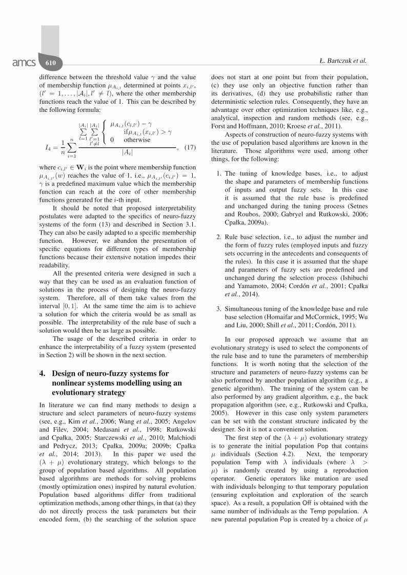
As explained in Section 2, the aim of the fuzzysystem described by rules of the form (37) is togenerate the values of coefficients of the matrix PA.For this reason, in Eqn. (37) the system outputs areindicated as p12 and p21. The obtained membershipfunctions are shown in Fig. 4(a) and the values of theinterpretability criteria in Table 1. As can be seen,the obtained fuzzy sets overlap significantly. For thisreason, it is difficult to associate a linguistic labelwith a clear interpretation, and the rules are difficultto read despite their small number.

For the second simulation conducted for thisproblem, aimed at gaining a system with thegreatest accuracy while observing the conditions ofinterpretability, the obtained results can be summarizedas follows:

• The accuracy of the model was RMSE = 0.0090and the maximum absolute error for input x1 wasx1 = 0.0246 and for input x2 it was x2 = 0.0155.The obtained result is, as would be expected, worsethan for the system described in the first variant (thesystem oriented on accuracy). However, it should benoted that the maximum absolute error was lowerthan 3% of the absolute value of the input signal,which can be considered a satisfactory result (seeFig. 3).

• A detailed form of fuzzy rules of the system (13)selected using the evolutionary strategy can berepresented as follows:


Fig. 4. Input and output fuzzy sets of the system used for modelling the harmonic oscillator in the case of high accuracy learning (a)as well as high interpretability and accuracy learning (b).

⎧⎪⎪⎪⎪⎪⎪⎨⎪⎪⎪⎪⎪⎪⎩

R1 :

IF x1 IS near(0.98)THEN p12 IS high AND p21 IS low,

R2 :

IF x1 IS near(−0.83)THEN p12 IS high AND p21 IS low,

R3 :

IF x1 IS near(0.01)THEN p12 IS low AND p21 IS high.

(38)

As in the case of the first simulation, the systemwas composed of three rules, but used only oneinput x1. Additionally, the obtained membershipfunctions were uniformly divided in the value spacesand overlapped each other to a much smaller degree,increasing the possibility of their interpretation(this is confirmed by the values obtained for eachinterpretability criterion presented in Table 1). Thereduction of the complexity of the system and theability to assign easily distinguishable linguisticlabels made this system much easier to read than theone obtained in the previous simulation.

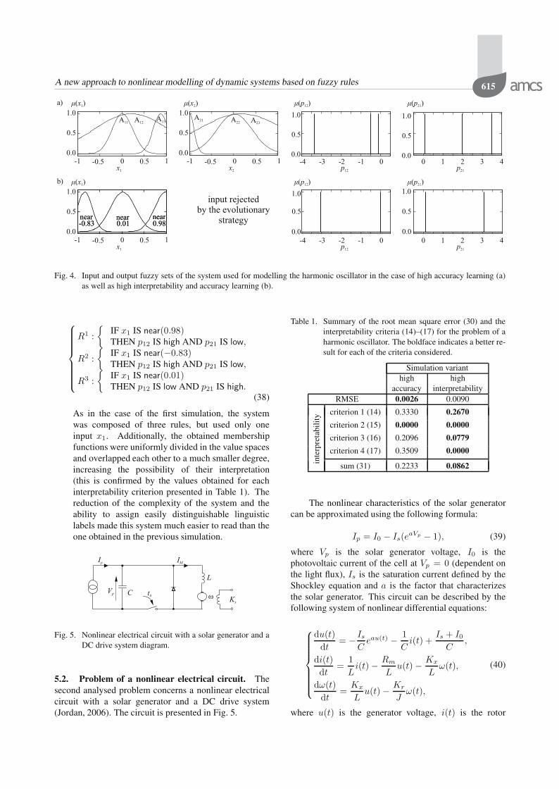
Fig. 5. Nonlinear electrical circuit with a solar generator and aDC drive system diagram.

5.2. Problem of a nonlinear electrical circuit. Thesecond analysed problem concerns a nonlinear electricalcircuit with a solar generator and a DC drive system(Jordan, 2006). The circuit is presented in Fig. 5.

Table 1. Summary of the root mean square error (30) and theinterpretability criteria (14)–(17) for the problem of aharmonic oscillator. The boldface indicates a better re-sult for each of the criteria considered.

Simulation varianthigh high

accuracy interpretabilityRMSE 0.0026 0.0090

inte

rpre

tabi

lity

criterion 1 (14) 0.3330 0.2670

criterion 2 (15) 0.0000 0.0000

criterion 3 (16) 0.2096 0.0779

criterion 4 (17) 0.3509 0.0000

sum (31) 0.2233 0.0862

The nonlinear characteristics of the solar generatorcan be approximated using the following formula:

Ip = I0 − Is(eaVp − 1), (39)

where Vp is the solar generator voltage, I0 is thephotovoltaic current of the cell at Vp = 0 (dependent onthe light flux), Is is the saturation current defined by theShockley equation and a is the factor that characterizesthe solar generator. This circuit can be described by thefollowing system of nonlinear differential equations:

⎧⎪⎪⎪⎪⎪⎪⎨⎪⎪⎪⎪⎪⎪⎩

du(t)

dt= −Is

Ceau(t) − 1

Ci(t) +

Is + I0C

,

di(t)

dt=

1

Li(t)− Rm

Lu(t)− Kx

Lω(t),

dω(t)

dt=

Kx

Lu(t)− Kr

Jω(t),

(40)

where u(t) is the generator voltage, i(t) is the rotor


Fig. 6. Graphical illustration of the reference signals (I–III) and the results of modelling the nonlinear electrical circuit by the fuzzysystem (13) in the case of high accuracy (panels 1(a)–1(c)) and high interpretability (panels 2(a)–2(c)) Panels 1(a) and 2(a)show the error obtained for signal u, 1(b) and 2(b) the error obtained for signal i, and 1(c) and 2(c) the error obtained forsignal ω.

current and ω(t) is the DC motor rotational speed.The parameters of circuit were set as follows: Rm =12.045Ω, C = 500μF, L = 0.1H, a = 0.54V−1,Kr =0.1Vs2, I0 = 2A, J = 10−3Ws3, Is = 1.28 ·10−5A, Vp = 22.15V,Kx = 0.5Vs. The values weretaken from the work of Jordan (2006). The values ofthe system matrix were determined using Taylor’s seriesexpansion method at point x = [22.15, 0.00, 0.00]T andare follows:

A =

⎡⎣ −2163.86 2000.00 0.00

10.00 −120.45 −5.000.00 500.00 −100.00

⎤⎦ . (41)

It should be noted that in the formulae (40) thenonlinearity occurs in the first of the equations in the partconcerning the generator voltage. We assume that weknow where the nonlinearity occurs but we do not knowits characteristics, so the correction matrix is defined bythe following formula:

PA =

⎡⎣ p11 0 0

0 0 00 0 0

⎤⎦ . (42)

The results obtained in the first (focused on accuracy)simulation can be summarized as follows:

• The accuracy of the model was RMSE = 0.0026.For signals u, i and ω, the maximum absolute errorswere εu = 0.0122 V, εi = 0.0001 A and εω =0.0002 rad/s, respectively (see Fig. 6). Thus, it can beconcluded that the prepared model well reproducesthe actual signals.

• A detailed form of fuzzy rules of the system(13) selected by the evolutionary strategy can bepresented as

⎧⎪⎪⎪⎪⎪⎪⎪⎪⎪⎪⎨⎪⎪⎪⎪⎪⎪⎪⎪⎪⎪⎩

R1 :

IF u ISAu4 AND i ISAi1 AND ω ISAω1

THEN p11 IS B1,

R2 :


THEN p11 IS B3,

R3 :


THEN p11 IS B4,

R4 :


THEN p11 IS B2.(43)

The shapes of membership functions are presented inFig. 7(a). As in the problem considered previously,the obtained functions highly overlap, making it


difficult to interpret and impossible to associateclear linguistic labels with fuzzy sets. Thus, thefuzzy rules (43) are difficult to read. The valuesof each interpretability criterion given by (14)–(17)are presented in Table 2. This justifies the needto include these criteria in the fuzzy system designprocess.

In the second group of simulations conducted forthe problem considered, the best obtained model can becharacterized by the following properties:

• The accuracy of the model was RMSE = 0.0083.For signals u, i and ω, the maximum absoluteerrors were εu = 0.0384 V, εi = 0.0013 A andεω = 0.0039 rad/s, respectively (see Fig. 6). Fromthis it can be concluded that the error rate slightlyincreased; however, the resulting accuracy is still at asatisfactory level.

• A detailed form of fuzzy rules of the system(13) selected by the evolutionary strategy can bepresented as

⎧⎪⎪⎨⎪⎪⎩R1 :

IF u IS near(19.00)AND i IS near(1.37)THEN p11 IS high,

R2 :

IF u IS near(22.69)AND i IS near(0.00)THEN p11 IS low.

(44)

The shapes of membership functions are presentedin Fig. 7(b). Those functions are characterized bya high degree of interpretability (as confirmed bythe values obtained for the different criteria listedin Table 2), allowing us to assign clear linguisticlabels to these functions. In addition, it should benoted that during the evolutionary process the createdfuzzy system consisted only of two rules and usedtwo inputs. This resulted in a significant decrease inthe system complexity and a further increase in itsreadability.

6. Conclusions

In this paper a new method of modelling a nonlineardynamic system was presented. It is based on combiningthe state-space modelling approach with methods ofcomputational intelligence. In particular, it uses thepossibilities of neuro-fuzzy systems to generate the valuesof the correction matrix, at each new operating point,which are added to the system matrix. This solutionenables more accurate modelling of systems in thoseareas where their characteristics are nonlinear. Todetermine the system structure and the parameters ofmembership functions, the (λ + μ) evolutionary strategywas used. An important element of the proposed methodis taking into account different interpretability criteria

Table 2. Summary of the root mean square error (30) and theinterpretability criteria (14)–(17) for the problem of anonlinear electrical circuit. The bold type indicates abetter result for each of the criteria considered.

Simulation varianthigh high

accuracy interpretabilityRMSE 0.0026 0.0083

inte

rpre

tabi

lity

criterion 1 (14) 0.4440 0.1780

criterion 2 (15) 0.0000 0.0000

criterion 3 (16) 0.2099 0.0000

criterion 4 (17) 0.4693 0.0305

sum5 (31) 0.2808 0.0520

in the fuzzy system design process. This resulted insystems with lower complexity, greater readability offuzzy rules included in the rule base, and operating withacceptable accuracy. This also makes it possible to assignspecific linguistic labels to fuzzy sets. The effectivenessof the proposed method was confirmed by the performedsimulations.

Acknowledgment

The authors would like to thank the reviewers for veryhelpful suggestions and comments in the revision process.

The project was financed by the PolishNational Science Center on the basis of the decisionDEC-2012/05/B/ST7/02138.

ReferencesAdjrad, M. and Belouchrani, A. (2007). Estimation of

multicomponent polynomial-phase signals impinging on amultisensor array using state-space modeling, IEEE Trans-actions on Signal Processing 55(1): 32–45.

Angelov, P.P., Filev, D.P. (2004). Flexible models with evolvingstructure, International Journal of Intelligent Systems19(4): 327–340.

Babuska, R., Verbruggen, H. (2003). Flexible neuro-fuzzymethods for nonlinear system identification, Annual Re-views in Control 27(1): 73–85.

Bagarinao, E., Matsuo, K., Nakai, T. and Sato, S. (2003).Estimation of general linear model coefficients forreal-time application, NeuroImage 19(2): 422–429.

Banerjee, A., Arkun, Y., Ogunnaike, B. and Pearson, R. (1997).Estimation of nonlinear systems using linear multiplemodels, AIChE Journal 43(5): 1204–1226.

Bohlin, T.P. (2006). Practical Grey-Box Process Identification:Theory and Applications, Springer, London.

Boukezzoula, R., Galichet, S. and Foulloy, L. (2007). Fuzzyfeedback linearizing controller and its equivalence with the


Fig. 7. Graphical illustration of fuzzy sets used in the fuzzy system (13) which is employed for modelling the nonlinear electricalcircuit in the case of high accuracy (a) and high interpretability (b). Since in the second case the input ω is not used, we do notpresent its fuzzy partition.

fuzzy nonlinear internal model control structure, Interna-tional Journal of Applied Mathematics and Computer Sci-ence 17(2): 233–248, DOI: 10.2478/v10006-007-0021-4.

Casillas, J., Cordón, O., Herrera, F. and Magdalena, L.(2003). Interpretability improvements to find the balanceinterpretability-accuracy in fuzzy modeling: An overview,in J. Casillas et al. (Eds.), Interpretability Issues in FuzzyModeling, Springer, Berlin/Heidelberg, pp. 3–22.

Caughey, T.K. (1963). Equivalent linearization techniques,Journal of the Acoustical Society of America35(11): 1706–1711.

Cordón, O. (2011). A historical review of evolutionary learningmethods for Mamdani-type fuzzy rule-based systems:Designing interpretable genetic fuzzy systems, Interna-tional Journal of Approximate Reasoning 52(6): 894–913.

Cordón, O., Herrera, F., Hoffmann, F. and Magdalena,L. (2001). Genetic Fuzzy Systems, World ScientificPublishing Company, Singapore.

Cpałka, K. (2009a). A new method for design and reduction ofneuro-fuzzy classification systems, IEEE Transactions onNeural Networks 20(4): 701–714.

Cpałka, K. (2009b). On evolutionary designing and learning offlexible neuro-fuzzy structures for nonlinear classification,Nonlinear Analysis A: Theory, Methods and Applications71(12): 1659–1672.

Cpałka, K., Łapa, K., Przybył, A. and Zalasinski, M. (2014).A new method for designing neuro-fuzzy systems fornonlinear modelling with interpretability aspects, Neuro-computing 135: 203–217.

Cpałka, K., Rebrova, O., Nowicki, R. and Rutkowski, L.(2013). On design of flexible neuro-fuzzy systems fornonlinear modelling, International Journal of General Sys-tems 42(6): 706–720.

Czekalski, P. (2006). Evolution-fuzzy rule based system withparameterized consequences, International Journal of Ap-plied Mathematics and Computer Science 16(3): 373–385.

DeHaan, D. and Guay, M. (2006). A new real-time perspectiveon non-linear model predictive control, Journal of ProcessControl 16(6): 615–624.

Di Nuovo, A. and Ascia, G. (2013). A fuzzy system indexto preserve interpretability in deep tuning of fuzzy rulebased classifiers, Journal of Intelligent and Fuzzy Systems25(2): 493–504.

Eiben, A.E. and Smith, J. (2008). Introduction to EvolutionaryComputing, Springer, Berlin/Heidelberg.

Fei, X., Lu, C.-C. and Liu, K. (2011). A Bayesian dynamiclinear model approach for real-time short-term freewaytravel time prediction, Transportation Research C: Emerg-ing Technologies 19(6): 1306–1318.

Fogel, D.B. (2006). Evolutionary Computation: Toward a NewPhilosophy of Machine Intelligence, Vol. 1, John Wiley &Sons, Hoboken, NJ.

Fogel, D.B. and Atmar, J.W. (1990). Comparing geneticoperators with Gaussian mutations in simulatedevolutionary processes using linear systems, Biologi-cal Cybernetics 63(2): 111–114.

Forst, W. and Hoffmann, D. (2010). Optimization Theory andPractice, Springer, New York, NY.

Gabryel, M. and Rutkowski, L. (2006). Evolutionary learningof Mamdani-type neuro-fuzzy systems, in L. Rutkowskiet al. (Eds.), Artificial Intelligence and Soft Computing,Lecture Notes in Computer Science, Vol. 4029, Springer,Berlin/Heidelberg, pp. 354–359.

Gacto, M., Alcala, R. and Herrera, F. (2011). Interpretabilityof linguistic fuzzy rule-based systems: An overview ofinterpretability measures, Information Sciences 181(20):4340–4360.

Grabowski, P. and Callier, F.M. (2001). Circle criterion andboundary control systems in factor form: Input-outputapproach, Applied Mathematics and Computer Science11(6): 1387–1403.


Háber, R. and Keviczky, L. (1999). Nonlinear Sys-tem Identification—Input-Output Modeling Approach, Vol.1: Nonlinear System Parameter Identification, SpringerNetherlands, Dordrecht.

Homaifar, A. and McCormick, E. (1995). Simultaneous designof membership functions and rule sets for fuzzy controllersusing genetic algorithms, IEEE Transactions on Fuzzy Sys-tems 3(2): 129–139.

Horzyk, A. and Tadeusiewicz, R. (2004). Self-optimizingneural networks, Advances in Neural Networks, Springer,Berlin/Heidelberg, pp. 150–155.

Huijberts, H., Nijmeijer, H. and Willems, R. (2000). Systemidentification in communication with chaotic systems,IEEE Transactions on Circuits and Systems I: Fundamen-tal Theory and Applications 47(6): 800–808.

Ikonen, E. and Najim, K. (2001). Advanced Process Identifica-tion and Control, Vol. 9, CRC Press, New York, NY.

Ishibashi, R. and Lucio Nascimento, Jr., C. (2013).GFRBS-PHM: A genetic fuzzy rule-based system forPHM with improved interpretability, IEEE Conference onPrognostics and Health Management, 2013, Gaithersburg,MD, USA, pp. 1–7.

Ishibuchi, H. and Yamamoto, T. (2004). Fuzzy rule selectionby multi-objective genetic local search algorithms and ruleevaluation measures in data mining, Fuzzy Sets and Sys-tems 141(1): 59–88.

Jang, I.-S. R. and Sun, C.-T. (1995). Neuro-fuzzy modeling andcontrol, Proceedings of the IEEE 83(3): 378–406.

Johansen, T.A., Shorten, R. and Murray-Smith, R. (2000).On the interpretation and identification of dynamicTakagi–Sugeno fuzzy models, IEEE Transactions on FuzzySystems 8(3): 297–313.

Johansson, U., Sönströd, C., Norinder, U. and Boström, H.(2011). Trade-off between accuracy and interpretability forpredictive in silico modeling, Future Medicinal Chemistry3(6): 647–663.

Jordan, A. (2006). Linearization of non-linear state equation,Bulletin of the Polish Academy of Sciences: Technical Sci-ences 54(1): 63–73.

Juang, C.-F. and Chen, C.-Y. (2013). Data-driven intervaltype-2 neural fuzzy system with high learning accuracyand improved model interpretability, IEEE Transactions onCybernetics 43(6): 1781–1795.

Kim, M.-S., Kim, C.-H. and Lee, J.-J. (2006). Evolving compactand interpretable Takagi–Sugeno fuzzy models with a newencoding scheme, IEEE Transactions on Systems, Man,and Cybernetics B: Cybernetics 36(5): 1006–1023.

Kluska, J. (2009). Analytical Methods in Fuzzy Modeling andControl, Springer, Berlin/Heidelberg.

Kluska, J. (2015). Selected applications of P1-TS fuzzyrule-based systems, in L. Rutkowski et al. (Eds.), Arti-ficial Intelligence and Soft Computing, Lecture Notes inComputer Science, Vol. 9119, Springer, Berlin/Heidelberg,pp. 195–206.

Kristensen, N.R., Madsen, H. and Jørgensen, S.B. (2004).A method for systematic improvement of stochasticgrey-box models, Computers & Chemical Engineering28(8): 1431–1449.

Kroese, D.P., Taimre, T. and Botev, Z.I. (2011). Handbookof Monte Carlo Methods, Vol. 706, John Wiley & Sons,Hoboken, NJ.

Li, C. and Chiang, T.-W. (2012). Intelligent financial timeseries forecasting: A complex neuro-fuzzy approach withmulti-swarm intelligence, International Journal of AppliedMathematics and Computer Science 22(4): 787–800, DOI:10.2478/v10006-012-0058-x.

Ljung, L. (2010). Approaches to identification of nonlinearsystems, 9th Chinese Control Conference, Beijing, China,pp. 1–5.

Łeski, J. (2003). A fuzzy if-then rule-based nonlinear classifier,International Journal of Applied Mathematics and Com-puter Science 13(2): 215–223.

Lughofer, E. (2013). On-line assurance of interpretabilitycriteria in evolving fuzzy systems—achievements,new concepts and open issues, Information Sciences251: 22–46.

Malchiodi, D. and Pedrycz, W. (2013). Learning membershipfunctions for fuzzy sets through modified support vectorclustering, in F. Masulli et al. (Eds.), Fuzzy Logic and Ap-plications, Springer, Cham, pp. 52–59.

Medasani, S., Kim, J. and Krishnapuram, R. (1998). Anoverview of membership function generation techniquesfor pattern recognition, International Journal of Approxi-mate Reasoning 19(3): 391–417.

Miller, G.A. (1956 ). The magical number seven, plus orminus two: Some limits on our capacity for processinginformation, The Psychological Review 63: 81–97.

Mrugalski, M. (2014). Advanced Neural Network-Based Com-putational Schemes for Robust Fault Diagnosis, Studiesin Computational Intelligence, Vol. 510, Springer-Verlag,Berlin/Heidelberg.

Murray-Smith, R. and Johansen, T. (1997). Multiple Model Ap-proaches to Nonlinear Modelling and Control, CRC Press,Boca Raton, FL.

Nelles, O. (2001). Nonlinear System Identification: From Clas-sical Approaches to Neural Networks and Fuzzy Models,Springer, Berlin/Heidelberg.

Ogata, K. (2004). System Dynamics, Pearson/Prentice Hall,Upper Saddle River, NJ.

Patton, R.J., Korbicz, J., Witczak, M. and Uppal, F.(2005). Combined computational intelligence andanalytical methods in fault diagnosis, IEE Control Engi-neering Series 70: 349.

Pedro, J.O. and Dahunsi, O.A. (2011). Neural network basedfeedback linearization control of a servo-hydraulic vehiclesuspension system, International Journal of Applied Math-ematics and Computer Science 21(1): 137–147, DOI:10.2478/v10006-011-0010-5.


Przybył, A. and Jelonkiewicz, J. (2003). Genetic algorithm forobserver parameters tuning in sensorless induction motordrive, Proceedings of the 6th International Conference onNeural Networks and Soft Computing, Zakopane Poland,pp. 376–381.

Puig, V., Witczak, M., Nejjari, F., Quevedo, J. and Korbicz,J. (2007). A GMDH neural network-based approach topassive robust fault detection using a constraint satisfactionbackward test, Engineering Applications of Artificial Intel-ligence 20(7): 886–897.

Quah, K.H. and Quek, C., (2006). FITSK: Online locallearning with generic fuzzy input Takagi–Sugeno–Kangfuzzy framework for nonlinear system estimation, IEEETransactions on Systems, Man, and Cybernetics B: Cyber-netics 36(1): 166-178.

Roffel, B. and Betlem, B.H. (2004). Advanced Practical ProcessControl, Springer, Berlin/Heidelberg.

Rüping, S. (2006). Learning Interpretable Models, Ph.D. thesis,Technical University of Dortmund, Dortmund.

Rutkowski, L. (2008). Computational Intelligence: Methods andTechniques, Springer, Berlin/Heidelberg.

Rutkowski, L. and Cpałka, K. (2005). Designing and learningof adjustable quasi-triangular norms with applications toneuro-fuzzy systems, IEEE Transactions on Fuzzy Systems13(1): 140–151.

Salapa, K., Trawinska, A., Roterman, I. and Tadeusiewicz, R.(2014). Speaker identification based on artificial neuralnetworks. Case study: The Polish vowel (a pilot study),Bio-Algorithms and Med-Systems 10(2): 91–99.

Setnes, M. and Roubos, H. (2000). GA-fuzzy modeling andclassification: Complexity and performance, IEEE Trans-actions on Fuzzy Systems 8(5): 509–522.

Schröder, D. (Ed.) (2000). Intelligent Observer and Control De-sign for Nonlinear Systems, Springer, Berlin/Heidelberg.

Shill, P., Akhand, M. and Murase, K. (2011). Simultaneousdesign of membership functions and rule sets for type-2fuzzy controllers using genetic algorithms, 14th Interna-tional Conference on Computer and Information Technol-ogy, Dhaka, Bangladesh, pp. 554–559.

Shukla, P. and Tripathi, S. (2013). Interpretability issuesin evolutionary multi-objective fuzzy knowledge basesystems, 7th International Conference on Bio-InspiredComputing: Theories and Applications, Madhya Pradesh,India, pp. 473–484.

Sivanandam, S. and Deepa, S. (2008). Genetic Algorithm Opti-mization Problems, Springer, Berlin/Heidelberg.

Starczewski, J.T., Bartczuk, Ł., Dziwinski, P. and Marvuglia, A.(2010). Learning methods for type-2 FLS based on FCM,in L. Rutkowski et al. (Eds.), Artificial Intelligence andSoft Computing, Springer, Berlin/Heidelberg, pp. 224–231.

Tadeusiewicz, R. (2010). Using neural networks forsimplified discovery of some psychological phenomena, inL. Rutkowski et al. (Eds.), Artificial Intelligence and SoftComputing, Springer, Berlin/Heidelberg, pp. 104–123.

Tadeusiewicz, R., Chaki, R. and Chaki, N. (2014). ExploringNeural Networks with C#, CRC Press, Boca Raton, FL.

Tadeusiewicz, R. and Figura, I. (2011). Phenomenon oftolerance to damage in artificial neural networks, Com-puter Methods in Materials Science 11(4): 501–513.

Tan, Y. (2004). Time-varying time-delay estimation fornonlinear systems using neural networks, InternationalJournal of Applied Mathematics and Computer Science14(1): 63–68.

Wang, H., Kwong, S., Jin, Y., Wei, W. and Man, K.-F. (2005).Agent-based evolutionary approach for interpretablerule-based knowledge extraction, IEEE Transactions onSystems, Man, and Cybernetics C: Applications and Re-views 35(2): 143–155.

Wang, H., Kwong, S., Jin, Y., Wei, W. and Man, K.-F.(2005). Multi-objective hierarchical genetic algorithm forinterpretable fuzzy rule-based knowledge extraction, FuzzySets and Systems 149(1): 149–186.

Wilamowski, B.M. (2005). Methods of computationalintelligence for nonlinear control systems, ICCAE 2005 In-ternational Conference on Control, Automation and Sys-tem, Gyeonggi-Do, Korea, pp. P1–P8.

Witkowska, A. and Smierzchalski, R. (2012). Designinga ship course controller by applying the adaptivebackstepping method, International Journal of AppliedMathematics and Computer Science 22(4): 985–997, DOI:10.2478/v10006-012-0073-y.

Wu, C.-J. and Liu, G.-Y. (2000). A genetic approach forsimultaneous design of membership functions and fuzzycontrol rules, Journal of Intelligent and Robotic Systems28(3): 195–211.

Xie, Y., Guo, B., Xu, L., Li, J. and Stoica, P. (2006).Multistatic adaptive microwave imaging for early breastcancer detection, IEEE Transactions on Biomedical Engi-neering 53(8): 1647.

Zhou, S.-M., Gan, J. Q. (2008). Low-level interpretability andhigh-level interpretability: A unified view of data-driveninterpretable fuzzy system modelling, Fuzzy Sets and Sys-tems 159(23): 3091–3131.

Łukasz Bartczuk was born in Czestochowa,Poland, in 1979. He received the M.Sc. andPh.D. degrees in computer science in 2003 and2008, respectively, both from the CzestochowaUniversity of Technology. Since 2008 he hasbeen an assistant professor at the Institute ofComputational Intelligence there. He has pub-lished about 15 technical papers in conferenceproceedings and book chapters. His main fieldsof interests include fuzzy systems, evolutionary

algorithms, and hybrid methods.


Andrzej Przybył was born in Brzeziny, Poland,in 1972. He received the Ph.D. degree in auto-matic control and robotics from the Poznan Uni-versity of Technology, Poland, in 2003. He isan assistant professor at the Institute of Compu-tational Intelligence, Czestochowa University ofTechnology, Poland. He works on developingnew control methods used in mechatronic sys-tems. His research interests center around mo-tion control systems, real-time Ethernet, field-

programmable gate array (FPGA) devices, and soft computing algo-rithms for electrical drives. He has designed various microprocessors,digital signal processors, and FPGA-based embedded systems. He haspublished about 40 technical papers.

Krzysztof Cpałka was born in Czestochowa,Poland, in 1972. He received the M.Sc. de-gree in electrical engineering in 1997 and thePh.D. degree (with honors) in computer engineer-ing in 2002, both from the Czestochowa Univer-sity of Technology, Poland, and the D.Sc. de-gree in computer engineering from the SystemsResearch Institute of the Polish Academy of Sci-ences in 2010. Since 2010, he has been an asso-ciate professor in the Institute of Computational

Intelligence at the Czestochowa University of Technology. He has pub-lished over 80 technical papers in journals, conference proceedings, andbook chapters. His research interests include fuzzy systems, evolution-ary algorithms, and hybrid methods.

Received: 27 June 2015Revised: 21 January 2016Re-revised: 20 May 2016Accepted: 15 June 2016

A NEW APPROACH TO NONLINEAR MODELLING OF DYNAMIC SYSTEMS...

Documents

Transcript of A NEW APPROACH TO NONLINEAR MODELLING OF DYNAMIC SYSTEMS...