A New Approach to Lossy Compression and … compression problems in achievability; 2) establishes...
172
A New Approach to Lossy Compression and Applications to Security Chen Eva Song A Dissertation Presented to the Faculty of Princeton University in Candidacy for the Degree of Doctor of Philosophy Recommended for Acceptance by the Department of Electrical Engineering Advisers: Paul Cuff and H. Vincent Poor November 2015
Transcript of A New Approach to Lossy Compression and … compression problems in achievability; 2) establishes...
A New Approach to Lossy Compression and
Applications to Security
Chen Eva Song
A Dissertation
Presented to the Faculty
of Princeton University
in Candidacy for the Degree
of Doctor of Philosophy
Recommended for Acceptance
by the Department of
Electrical Engineering
Advisers: Paul Cuff and H. Vincent Poor
November 2015

c© Copyright by Chen Eva Song, 2015.
All rights reserved.
Abstract
In this thesis, rate-distortion theory is studied in the context of lossy compression commu-
nication systems with and without security concerns. A new source coding proof technique
using the “likelihood encoder” is proposed that achieves the best known compression rate in
various lossy compression settings. It is demonstrated that the use of the likelihood encoder
together with Wyner’s soft-covering lemma yields simple achievability proofs for classical
source coding problems. We use the likelihood encoder technique to show the achievability
parts of the point-to-point rate-distortion function, the rate-distortion function with side
information at the decoder (i.e. the Wyner-Ziv problem), and the multi-terminal source
coding inner bound (i.e. the Berger-Tung problem). Furthermore, a non-asymptotic analy-
sis is used for the point-to-point case to examine the upper bound on the excess distortion
provided by this method. The likelihood encoder is also compared, both in concept and
performance, to a recent alternative random-binning based technique.
Also, the likelihood-encoder source coding technique is further used to obtain new results
in rate-distortion based secrecy systems. Several secure source coding settings, such as using
shared secret key and correlated side information, are investigated. It is shown that the
rate-distortion based formulation for secrecy fully generalizes the traditional equivocation-
based secrecy formulation. The extension to joint source-channel security is also considered
using similar encoding techniques. The rate-distortion based secure source-channel analysis
is applied to optical communication for reliable and secure delivery of an information source
through a multimode fiber channel subject to eavesdropping.
iii

Acknowledgements
First and foremost, I would like to express my sincere gratitude to my advisors Prof. Paul
Cuff and Prof. Vincent Poor for their continuous selfless advice, encouragement and support
throughout the course of my thesis. They are the kindest coaches, colleagues, and friends
that always give me freedom of exploring new research.
I would like to thank my thesis reader and examiner, Prof. Sergio Verdu, for his in-
sightful comments and passion for perfection. My thanks also goes to the rest of my thesis
committee: Prof. Emmanuel Abbe and Prof. Prateek Mittal.
Uncountable interesting discussions and idea exchanges happened during the past
five years with my fellow labmates: Curt Schieler, Sai (Sanket) Satpathy, Jingbo Liu,
Sree(chakra) Goparaju, Rafael Schaefer, Samir Perlaza, Inaki Esnaola, Victoria Kostina,
Salim ElRouayheb, Sander Wahls, Ronit Bustin, Nino(slav) Marina, Yue Zhao, Giacomo
Bacci, Rene Guillaume, etc.
I would like to give very special thanks to my friends: Alex Xu, Cynthia Lu, Jiasi Chen,
and Mia Chen for laughing and crying with me whenever I need them.
I am thankful to the friendly staff in Department of Electrical Engineering and Princeton
University.
I really enjoyed the university resource – Baker Rink, which allowed me to start figure
skating during my time at Princeton and made my dream from childhood come true.
Finally, I take this opportunity to express my profound gratitude to my parents and my
husband Edward for their love, understanding and support – both spiritually and finan-
cially.
iv

To my parents.
v

Contents
Abstract . . . . . . . . . . . . . . . . . . . . . . . . . . . . . . . . . . . . . . . . . iii
Acknowledgements . . . . . . . . . . . . . . . . . . . . . . . . . . . . . . . . . . . iv
1 Introduction 1
1.1 Preview . . . . . . . . . . . . . . . . . . . . . . . . . . . . . . . . . . . . . . 1
2 Preliminaries 8
2.1 Notation . . . . . . . . . . . . . . . . . . . . . . . . . . . . . . . . . . . . . . 8
2.2 Distortion Measure . . . . . . . . . . . . . . . . . . . . . . . . . . . . . . . . 9
2.3 Total Variation Distance . . . . . . . . . . . . . . . . . . . . . . . . . . . . . 10
2.4 The Likelihood Encoder . . . . . . . . . . . . . . . . . . . . . . . . . . . . . 11
2.5 Soft-covering Lemmas . . . . . . . . . . . . . . . . . . . . . . . . . . . . . . 11
3 Point-to-point Lossy Compression 14
3.1 Introdution . . . . . . . . . . . . . . . . . . . . . . . . . . . . . . . . . . . . 14
3.2 Problem Formulation . . . . . . . . . . . . . . . . . . . . . . . . . . . . . . . 15
3.3 Achievability Using the Likelihood Encoder . . . . . . . . . . . . . . . . . . 16
3.4 Excess Distortion . . . . . . . . . . . . . . . . . . . . . . . . . . . . . . . . . 20
3.4.1 Probability of Excess Distortion . . . . . . . . . . . . . . . . . . . . 20
3.4.2 Non-asymptotic Performance . . . . . . . . . . . . . . . . . . . . . . 21
3.4.3 Comparison with Random Binning Based Proof . . . . . . . . . . . . 23
3.5 A Non-Asymptotic Analysis Using Jensen’s Inequality . . . . . . . . . . . . 34
3.6 Summary . . . . . . . . . . . . . . . . . . . . . . . . . . . . . . . . . . . . . 36
vi

4 Multiuser Lossy Compression 38
4.1 Introduction . . . . . . . . . . . . . . . . . . . . . . . . . . . . . . . . . . . . 38
4.2 Approximation Lemma . . . . . . . . . . . . . . . . . . . . . . . . . . . . . . 39
4.3 The Wyner-Ziv Setting . . . . . . . . . . . . . . . . . . . . . . . . . . . . . . 39
4.3.1 Problem Formulation . . . . . . . . . . . . . . . . . . . . . . . . . . 39
4.3.2 Proof of Achievability . . . . . . . . . . . . . . . . . . . . . . . . . . 41
4.4 The Berger-Tung Inner Bound . . . . . . . . . . . . . . . . . . . . . . . . . 46
4.4.1 Problem Formulation . . . . . . . . . . . . . . . . . . . . . . . . . . 46
4.4.2 Proof of Achievability . . . . . . . . . . . . . . . . . . . . . . . . . . 48
4.5 Summary . . . . . . . . . . . . . . . . . . . . . . . . . . . . . . . . . . . . . 54
5 Rate-Distortion Based Security in the Noiseless Wiretap Channel 55
5.1 Introduction . . . . . . . . . . . . . . . . . . . . . . . . . . . . . . . . . . . . 55
5.2 Secure Source Coding Via Secret Key . . . . . . . . . . . . . . . . . . . . . 56
5.2.1 The Shannon Cipher System and Perfect Secrecy . . . . . . . . . . . 56
5.2.2 Naive Rate-Distortion Based Secrecy . . . . . . . . . . . . . . . . . . 58
5.3 Secure Source Coding with Side Information at the Decoders . . . . . . . . 60
5.3.1 Problem Formulation . . . . . . . . . . . . . . . . . . . . . . . . . . 61
5.3.2 Inner Bound . . . . . . . . . . . . . . . . . . . . . . . . . . . . . . . 63
5.3.3 Outer Bound . . . . . . . . . . . . . . . . . . . . . . . . . . . . . . . 72
5.3.4 Special Cases . . . . . . . . . . . . . . . . . . . . . . . . . . . . . . . 73
5.3.5 Example . . . . . . . . . . . . . . . . . . . . . . . . . . . . . . . . . . 74
5.4 Secure Source Coding with Causal Disclosure . . . . . . . . . . . . . . . . . 76
5.4.1 Problem Formulation . . . . . . . . . . . . . . . . . . . . . . . . . . 77
5.4.2 Main Results . . . . . . . . . . . . . . . . . . . . . . . . . . . . . . . 79
5.4.3 Equivocation . . . . . . . . . . . . . . . . . . . . . . . . . . . . . . . 79
5.4.4 Binary Source . . . . . . . . . . . . . . . . . . . . . . . . . . . . . . . 81
5.4.5 Gaussian Source . . . . . . . . . . . . . . . . . . . . . . . . . . . . . 81
5.5 Summary . . . . . . . . . . . . . . . . . . . . . . . . . . . . . . . . . . . . . 89
vii
6 Source-Channel Security in the Noisy Wiretap Channel 91
6.1 Introduction . . . . . . . . . . . . . . . . . . . . . . . . . . . . . . . . . . . . 91
6.2 Operational Separate Source-Channel Security . . . . . . . . . . . . . . . . 92
6.2.1 Naive Formulation . . . . . . . . . . . . . . . . . . . . . . . . . . . . 92
6.2.2 With Causal Source Disclosure at the Eavesdropper . . . . . . . . . 101
6.2.3 Binary Symmetric Broadcast Channel and Binary Source . . . . . . 113
6.2.4 Applications to Multimode Fiber . . . . . . . . . . . . . . . . . . . . 114
6.3 Joint Source-Channel Security . . . . . . . . . . . . . . . . . . . . . . . . . . 122
6.3.1 Problem Revisit . . . . . . . . . . . . . . . . . . . . . . . . . . . . . 122
6.3.2 Secure Hybrid Coding . . . . . . . . . . . . . . . . . . . . . . . . . . 124
6.3.3 Scheme Comparision . . . . . . . . . . . . . . . . . . . . . . . . . . . 130
6.3.4 The Perfect Secrecy Outer Bound . . . . . . . . . . . . . . . . . . . 131
6.3.5 Numerical Example . . . . . . . . . . . . . . . . . . . . . . . . . . . 132
6.4 Summary . . . . . . . . . . . . . . . . . . . . . . . . . . . . . . . . . . . . . 132
6.5 Appendix . . . . . . . . . . . . . . . . . . . . . . . . . . . . . . . . . . . . . 134
6.5.1 Proof of Lemma 6.1 . . . . . . . . . . . . . . . . . . . . . . . . . . . 134
6.5.2 Proof of Lemma 6.2 . . . . . . . . . . . . . . . . . . . . . . . . . . . 134
6.5.3 Proof of (6.24) . . . . . . . . . . . . . . . . . . . . . . . . . . . . . . 137
6.5.4 Justification of the condition max(Rs,Rp)∈RRs > 0 . . . . . . . . . . 138
6.5.5 Proof of Theorem 6.2 and Theorem 6.7 . . . . . . . . . . . . . . . . 138
6.5.6 Proof of Lemma 6.3 . . . . . . . . . . . . . . . . . . . . . . . . . . . 146
6.5.7 Sufficient condition on Theorem 6.11 . . . . . . . . . . . . . . . . . . 147
6.5.8 Proof of Theorem 6.15 . . . . . . . . . . . . . . . . . . . . . . . . . . 148
7 Conclusion 159
Bibliography 161
viii

Chapter 1
Introduction
1.1 Preview
Information theory, founded by Claude Shannon in 1948, has provided insights into the
fundamental issues in data compression and date transmission. In addition to data com-
pression and transmission, it has also impacted other areas such as cryptography, machine
learning, and computer networks over the decades.
This thesis focuses on the aspect of information theory that 1) re-approaches the lossy
data compression problems in achievability; 2) establishes the connection between secu-
rity and lossy data compression in communication systems. With the rise of big data in
analytics and data management, storing and transferring data reliably and securely has
become a critical issue. Secure communication can take one of two routes: cryptography
or information-theoretic secrecy. These areas are similar in the sense that both study how
to transmit data securely to an intended receiver in the presence of an adversary. While
cryptography deals with designing protocols and algorithms that make the ciphered text
computationally hard to break with current technology, information-theoretic secrecy tack-
les a more fundamental question by asking whether there exists an encryption scheme such
that the ciphered text is unbreakable even if the adversary is given unlimited computing
power. In this thesis, we consider this latter approach. However, our approach to analyzing
the security of a communication system is based on rate-distortion theory, which differs
from the traditional approach of information-theoretic secrecy; instead of measuring the
1
statistical dependence between the original information and the ciphered text (by a quan-
tity called equivocation), we use a distortion metric to evaluate how an adversary can make
the most use of the leaked information to form a sequence of actions against the intended
receiver. Traditional information-theoretic secrecy uses equivocation-rate to quantify the
level of security, which requires a large size of secret key to allow a non-negligible amount
of normalized equivocation. In our analysis of secure communication, although unlimited
computing power is still granted to the adversary, we allow the adversary to potentially learn
part of the ciphered text as long as the actions it can form are harmless to the intended
receiver. This relaxation is proven to significantly reduce the secret key size.
A highlight of this thesis is a tool called the “likelihood encoder” introduced in Chapter
2. The likelihood encoder is a source compressor that achieves optimum rate given by the
rate-distortion function for lossy compression. With this encoder, one is able to construct a
communication system that can be approximated by a much simpler distribution that makes
the analysis effortless. Although the likelihood encoder is mostly used to get new results
in secrecy settings in this thesis, its applications to classical source coding provide a very
different observation and treatment from other existing optimum rate achieving techniques.
Lossy Compression
Source coding, frequently referred to as data compression in applications, has been studied
for decades. Basic technologies, such as JPEG and MP3, are ubiquitous in data storage.
Traditionally, lossy compression in information theory studies the tradeoff between the rate
of compression and the quality of reconstruction in the fundamental limit (rate-distortion
theory) by allowing processing of the data in a big batch. An example of lossy compression
applied to image storage is given in Fig. 1.1.
In Chapter 3, we review the simplest setting for lossy compression – point-to-point lossy
compression. Within this simple setting, we provide a detailed step-by-step methodology
using the likelihood encoder as a lossy source compressor and its corresponding analysis.
This is the starting point to become familiarized with this tool, since the analysis for the
more complicated systems in later chapters are variations of this basic case.
2

encoder decoder
177792 bits 55064 bits
0111001 … 1000011
55064 bits
Figure 1.1: Lossy image compression: quality is traded off for size.
In Chapter 4, we extend the analysis using the likelihood encoder to more sophisticated
setups: lossy compression with side information at the decoder, a.k.a the Wyner-Ziv setting,
and multi-terminal lossy source compression with joint decoding, a.k.a. the Berger-Tung
setting.
Secure Source Coding
The goal of secure source coding is to simultaneously 1) compress data efficiently so that an
intended receiver can reconstruct the data with high fidelity and 2) encrypt the data in such
a way that an eavesdropper does not learn anything “meaningful” about the data. Here
the word “meaningful” has different interpretations. In Shannon’s formulation [1] of perfect
secrecy, in order to prevent the eavesdropper from learning “meaningful” information about
the data source S, it is required that the encrypted message M available to the eavesdropper
and the source are statistically independent, i.e. PS = PS|M . It turns out that, under
this formulation, a separation principle applies: one can achieve optimality simply by first
compressing the source with the most efficient compression algorithm and then encrypting
the compressed data with a one-time pad. Although it may appear that we do not lose any
efficiency in compression to the legitimate receiver, one should notice that this comes at the
additional cost of sharing common randomness between the transmitter and the legitimate
receiver, in this case, a shared secret key. Under the requirement for perfect secrecy, the
secret key needs to be at least the size of the compressed data. This motivates us to ask
the following questions: what if we only have a limited size of secret key? are we still able
3
to encrypt the data in a way that favors the legitimate users the most? These questions
lead us to investigate partial secrecy.
Perfect secrecy is so fundamental and simple that it could be expressed with many
different metrics. Information theorists like using entropy and mutual information, but
that doesn’t make it the correct way to state partial secrecy. The traditional approach to
information theoretic security in the partial secrecy regime simply adopts the same metric
for perfect secrecy. That is, instead of asking for H(S|M) = H(S) (under perfect secrecy),
one studies the tradeoff between the equivocation H(S|M) and the secret key size. Such
extension of using conditional entropy to measure partial secrecy is problematic in the
sense that it does not capture how the eavesdropper can make use of the information to
form actions against the legitimate users.
One may ask the question: if lossy reproduction is allowed at the legitimate receiver, why
not allow that the eavesdropper recovers a distorted version of the message? Yamamoto [2]
started reexamining the Shannon cipher system from a rate-distortion approach by studying
the tradeoff among efficiency of compression, secret key size and the “minimum distortion”
at the eavesdropper. Here the term “minimum distortion” simply means that, one should
assume a rational eavesdropper that reconstructs the source so as to minimize the distortion.
Under this formulation, the legitimate users (the transmitter and the legitimate receiver)
who get to design the communication protocol and the adversary (the eavesdropper) are put
in a game-theoretic setting, where they are playing a zero-sum game by properly choosing a
payoff function that captures the distortions from both the legitimate receiver and the eaves-
dropper. Therefore, from the system designer’s point of view, Yamamoto’s setup focuses
on finding a good encoding (compression and encryption) scheme under the assumption of
a rational eavesdropper. Since we no longer have the luxury of sufficient secret key size to
protect all of the data to achieve perfect secrecy, it becomes important to understand which
information bits to hide to benefit the legitimate users the most in the sense of forcing a
large distortion at the eavesdropper. Schieler and Cuff [3] showed that this relaxation of
the secrecy requirement greatly reduced the size of secret key needed.
However, the shortcomings of Yamamoto’s secrecy formulation for secrecy are exposed
under a careful examination. Yamamoto’s rate-distortion model of the Shannon cipher
4

system remains a valid game-theoretic setting if the legitimate receiver and the eavesdropper
are each given only one chance to reproduce the source. In reality, the eavesdropper may
have multiple chances to make its estimate. An intuitive example is the following. Suppose
the source is a black-and-white image, one-bit pixels. One can force the highest possible
distortion (under Hamming distortion) at the eavesdropper by simply flipping all the pixel
bits, shown in Fig. 1.2. Yet the eavesdropper actually learns so much about the source
that it can guarantee to decode the exact image within two attempts. Therefore, it may be
overoptimistic to consider Yamamoto’s model as secure source coding.
Figure 1.2: The Hamming distortion between the two images is at the maximum, but onecan fully recover one image from the other without any loss of information.
A patch for Yamamoto’s weak notion of security is provided by Cuff [4] [5] by allow-
ing the eavesdropper to have access to causal information about the source. To be more
intuitive, it is helpful to think under the game-theoretic setting where each player (trans-
mitter/legitimate receiver and the eavesdropper) takes a sequence of actions. When the
eavesdropper is calculating its current best move, it already observes the past moves of the
transmitter/legitimate receiver. It is obvious that this modification favors the eavesdropper
as it has the freedom to readjust its strategy after each move. Although this causal dis-
closure of the source may appear to be an unnatural reinforcement, it is shown by Schieler
and Cuff [6] that the causal disclosure is key to specify a stable secrecy model for source
coding that fully generalizes the traditional equivocation approach.
In Chapter 5, we discuss the rate-distortion based secure source coding in detail. We
start with a review of Shannon’s perfect secrecy formulation, followed by Yamamoto’s game-
5

theoretic formulation. We then investigate a variation of Yamamoto’s model by replacing
the secret key with side information. That is, instead of having a shared secret key between
the transmitter and the legitimate receiver, the legitimate receiver and the eavesdropper
are given different side information that is correlated with the source during decoding. This
is a good example of physical-layer security in source coding, where security is achieved by
exploiting the physical structure of the communication network without using any common
randomness explicitly. Finally, we strengthen the security model by considering causal
source disclosure to the eavesdropper. The mathematical relation between the equivocation
and the rate-distortion approaches is described.
Secure Source-Channel Coding
In joint source-channel coding, we want to compress the data by removing redundancy
and transmit it with high fidelity over a noisy channel by adding redundancy at the same
time. In the lucky cases such as point-to-point communication, where we have only one
data source and one receiver, it is well known in information theory that separating the
two processes (source coding and channel coding) is optimal when processing the data in a
big batch. In other words, one does not lose any efficiency in the communication by first
compressing the data source with the best compression algorithm and then structure the
compressed information bits for the channel using the best channel code. Unfortunately,
in the general cases of an arbitrary communication network, with and without security
concerns, separating these two processes is not optimal, not even in the point-to-point
communication from the non-asymptotic perspective.
For secure source-channel coding, physical-layer security also comes into play. Wyner
[7] pioneered the area of information theoretic secrecy by studying secure transmission of
data through a noisy broadcast channel, a.k.a. the wire-tap channel. In this setting, no
secret key is used and the security is established only by taking advantage of the proper-
ties of the channel itself. Naturally, the legitimate receiver’s channel needs to be stronger
than the eavesdropper’s channel in some sense to ensure secure transmission of the data;
otherwise, what is decodable to the legitimate receiver is also decodable to the eavesdrop-
per. Although physical-layer security is mainly studied in the context of secure channel
6

coding, many properties carry over to source-channel security. The obvious starting point
in considering the latter problem is to conduct secure source coding and secure channel
coding operationally separately. An operationally separate source-channel coding scheme is
still a joint source-channel coding scheme in the sense that the source encoder and channel
encoder need to first establish an agreement such that the output from the source encoder
meets certain requirements, but once those requirements are satisfied, the source encoder
and channel encoder have the freedom of choosing their own algorithms. Rarely is an op-
erationally separate scheme optimal in secure source-channel settings, which motivates us
to explore more sophisticated joint source-channel coding schemes.
A new joint source-channel coding approach was introduced in the context of multiuser
lossy communication by Minero et al. [8]. This joint coding technique is unique and simple
in the following aspects: 1) the source encoding and channel encoding operations decouple;
2) the same codeword is used for both source coding and channel coding; and 3) the scheme
achieves best known performance among existing joint source-channel coding schemes. This
hybrid coding is of particular interest because the structure of the code aligns well with our
likelihood encoder. Although hybrid coding was originally demonstrated with the standard
analysis using the joint-typicality encoder, the process can be greatly simplified by using the
corresponding analysis of the likelihood encoder. In this thesis, we focus on the application
of the hybrid coding technique to security in a wire-tap channel.
In Chapter 6, we discuss secure source-channel coding over a noisy wiretap channel
through physical-layer security. Following the footsteps from Chapter 5 for secure source
coding, we first study the operationally separate source-channel model under the rate-
distortion based game-theoretic setting without causal source disclosure and the stronger
secrecy setting by allowing causal source disclosure, respectively. We then apply the hybrid
coding scheme to the setting with causal source disclosure and compare results with the
operationally separate coding scheme.
7
Chapter 2
Preliminaries
2.1 Notation
A sequence X1, ..., Xn is denoted by Xn. Limits taken with respect to “n → ∞” are
abbreviated as “→n”. When X denotes a random variable, x is used to denote a realization,
X is used to denote the support of that random variable, and ∆X is used to denote the
probability simplex of distributions with alphabet X . A Markov relation is denoted by the
symbol −. We use EP and PP to indicate expectation and probability taken with respect
to a distribution P ; however, when the distribution is clear from the context, the subscript
will be omitted. To keep the notation uncluttered, the arguments of a distribution are
sometimes omitted when the arguments’ symbols match the subscripts of the distribution,
e.g. PX|Y (x|y) = PX|Y . We use a bold capital letter P to denote that a distribution P is
random (with respect to a random codebook).
In the analysis involving the likelihood encoder, P is reserved to denote the true in-
duced distribution of a communication system specified by a particular choice of encoder
and decoder. When PX is used to denote a single-letter distribution, PXn is reserved to
denote the independent and identically distributed (i.i.d.) process with marginal PX , i.e.
PXn(xn) =∏nt=1 PX(xt). We use R to denote the set of real numbers and R+ to denote
the nonnegative subset.
8

2.2 Distortion Measure
Definition 2.1. A distortion measure is a mapping
d : X × Y 7→ R+ (2.1)
from the set of source alphabet-reproduction alphabet pairs into the set of non-negative real
numbers.
Definition 2.2. The maximum distortion is defined as
dmax = max(x,y)∈X×Y
d(x, y). (2.2)
A distortion measure is said to be bounded if
dmax <∞. (2.3)
Definition 2.3. The distortion between two sequences is defined to be the per-letter average
distortion
d(xn, yn) =1
n
n∑t=1
d(xt, yt). (2.4)
Two common distortion measures that are used frequently in this thesis are given as
follows.
Definition 2.4. The Hamming distortion is given by
d(x, y) =
0 : x = y
1 : x 6= y(2.5)
Definition 2.5. The squared error distortion is given by
d(x, y) = (x− y)2. (2.6)
9
To measure the distortion of X incurred by representing it as Y , we use the expected
distortion E[d(X,Y )].
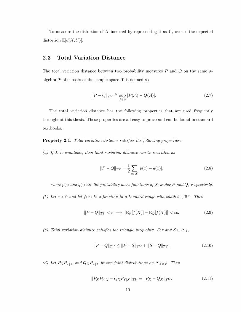
2.3 Total Variation Distance
The total variation distance between two probability measures P and Q on the same σ-
algebra F of subsets of the sample space X is defined as
‖P −Q‖TV , supA∈F|P (A)−Q(A)|. (2.7)
The total variation distance has the following properties that are used frequently
throughout this thesis. These properties are all easy to prove and can be found in standard
textbooks.
Property 2.1. Total variation distance satisfies the following properties:
(a) If X is countable, then total variation distance can be rewritten as
‖P −Q‖TV =1
2
∑x∈X|p(x)− q(x)|, (2.8)
where p(·) and q(·) are the probability mass functions of X under P and Q, respectively.
(b) Let ε > 0 and let f(x) be a function in a bounded range with width b ∈ R+. Then
‖P −Q‖TV < ε =⇒∣∣EP [f(X)]− EQ[f(X)]
∣∣ < εb. (2.9)
(c) Total variation distance satisfies the triangle inequality. For any S ∈ ∆X ,
‖P −Q‖TV ≤ ‖P − S‖TV + ‖S −Q‖TV . (2.10)
(d) Let PXPY |X and QXPY |X be two joint distributions on ∆X×Y . Then
‖PXPY |X −QXPY |X‖TV = ‖PX −QX‖TV . (2.11)
10

(e) For any P,Q ∈ ∆X×Y ,
‖PX −QX‖TV ≤ ‖PXY −QXY ‖TV . (2.12)
2.4 The Likelihood Encoder
We now define the likelihood encoder, operating at rate R, which receives a sequence
x1, ..., xn and maps it to a message M ∈ [1 : 2nR]. In normal usage, a decoder will then use
M to form an approximate reconstruction of the x1, ..., xn sequence.
The encoder is specified by a codebook of un(m) sequences and a joint distribution PUX .
Consider the likelihood function for each codeword, with respect to a memoryless channel
from U to X, defined as follows:
L(m|xn) , PXn|Un(xn|un(m)) =
n∏t=1
PX|U (xt|ut(m)). (2.13)
A likelihood encoder is a stochastic encoder that determines the message index with prob-
ability proportional to L(m|xn), i.e.
PM |Xn(m|xn) =L(m|xn)∑
m′∈[1:2nR] L(m′|xn)∝ L(m|xn). (2.14)
2.5 Soft-covering Lemmas
Now we introduce the core lemmas that serve as the foundation for analyzing several source
coding problems in both lossy compression and secrecy. One can consider the role of the
soft-covering lemma in analyzing the likelihood encoder as analogous to that of the joint
asymptotic equipartition property (J-AEP) which is used for the analysis of joint-typicality
encoders [9] [10]. The general idea of the soft-covering lemma is that the distribution
induced by selecting uniformly from a random codebook and passing the codeword through
a memoryless channel is close to an i.i.d. distribution as long as the codebook size is large
enough.
11
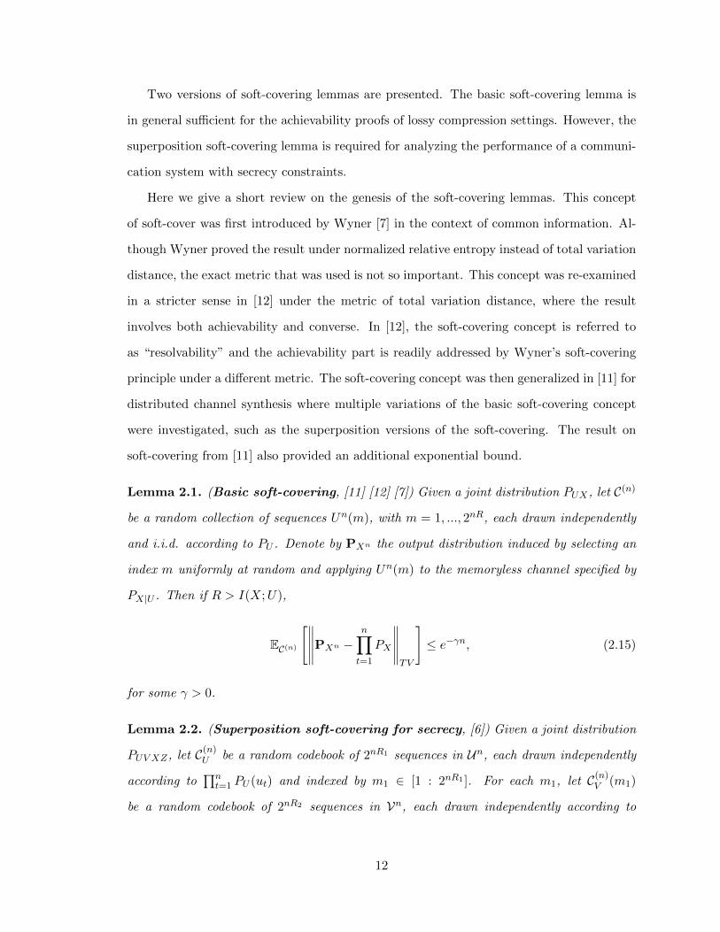
Two versions of soft-covering lemmas are presented. The basic soft-covering lemma is
in general sufficient for the achievability proofs of lossy compression settings. However, the
superposition soft-covering lemma is required for analyzing the performance of a communi-
cation system with secrecy constraints.
Here we give a short review on the genesis of the soft-covering lemmas. This concept
of soft-cover was first introduced by Wyner [7] in the context of common information. Al-
though Wyner proved the result under normalized relative entropy instead of total variation
distance, the exact metric that was used is not so important. This concept was re-examined
in a stricter sense in [12] under the metric of total variation distance, where the result
involves both achievability and converse. In [12], the soft-covering concept is referred to
as “resolvability” and the achievability part is readily addressed by Wyner’s soft-covering
principle under a different metric. The soft-covering concept was then generalized in [11] for
distributed channel synthesis where multiple variations of the basic soft-covering concept
were investigated, such as the superposition versions of the soft-covering. The result on
soft-covering from [11] also provided an additional exponential bound.
Lemma 2.1. (Basic soft-covering, [11] [12] [7]) Given a joint distribution PUX , let C(n)
be a random collection of sequences Un(m), with m = 1, ..., 2nR, each drawn independently
and i.i.d. according to PU . Denote by PXn the output distribution induced by selecting an
index m uniformly at random and applying Un(m) to the memoryless channel specified by
PX|U . Then if R > I(X;U),
EC(n)
[∥∥∥∥∥PXn −n∏t=1
PX
∥∥∥∥∥TV
]≤ e−γn, (2.15)
for some γ > 0.
Lemma 2.2. (Superposition soft-covering for secrecy, [6]) Given a joint distribution
PUV XZ , let C(n)U be a random codebook of 2nR1 sequences in Un, each drawn independently
according to∏nt=1 PU (ut) and indexed by m1 ∈ [1 : 2nR1 ]. For each m1, let C(n)
V (m1)
be a random codebook of 2nR2 sequences in Vn, each drawn independently according to
12

∏nt=1 PV |U (vt|ut(m1)) and indexed by (m1,m2) ∈ [1 : 2nR2 ]. Let
PM1M2XnZk(m1,m2, xn, zk)
, 2−n(R1+R2)n∏t=1
PX|UV (xt|Ut(m1), Vt(m1,m2))PZ|XUV (zt|xt, ut, vt)1{t∈[1:k]},(2.16)
and
QM1XnZk(m1, xn, zk)
, 2−nR1
n∏t=1
PX|U (xt|Ut(m1))PZ|XU (zt|xt, Ut(m1))1{t∈[1:k]} (2.17)
If R2 > I(X;V |U), then
EC(n)
[∥∥PM1XnZk −QM1XnZk∥∥TV
]≤ e−γn (2.18)
for any α < R2−I(X;V |U)I(Z;V |UX) , k ≤ αn, where γ > 0 depends on the gap R2−I(X;V |U)
I(Z;V |UX) − α.
13
Chapter 3
Point-to-point Lossy Compression
3.1 Introdution
Rate-distortion theory, founded by Shannon in [13] and [14], provides the fundamental
limits of lossy source compression. The minimum rate required to represent an i.i.d. source
sequence under a given tolerance of distortion is given by the rate-distortion function.
Standard proofs [9], [10] of achievability for these rate-distortion problems often use joint-
typicality encoding, i.e. the encoder looks for a codeword that is jointly typical with the
source sequence.
In this chapter, we propose using a likelihood encoder to achieve these source coding
results. The likelihood encoder is a stochastic encoder. As stated in [15], for a chosen joint
distribution PXY , to encode a source sequence x1, ..., xn (i.e. xn) with codebook yn(m), the
encoder stochastically chooses an index m proportional to the likelihood of yn(m) passed
through the memoryless “test channel” PX|Y .
The advantage of using such an encoder is that it naturally leads to an idealized distri-
bution which is simple to analyze, based on the “test channel.” The distortion performance
of the idealized distribution carries over to the true system induced distribution because
the two distributions are shown to be close in total variation.
The application of the likelihood encoder together with the soft-covering lemma is not
limited to only discrete alphabets. The proof for sources from continuous alphabets is
readily included, since the soft-covering lemma imposes no restriction on alphabet size.
14
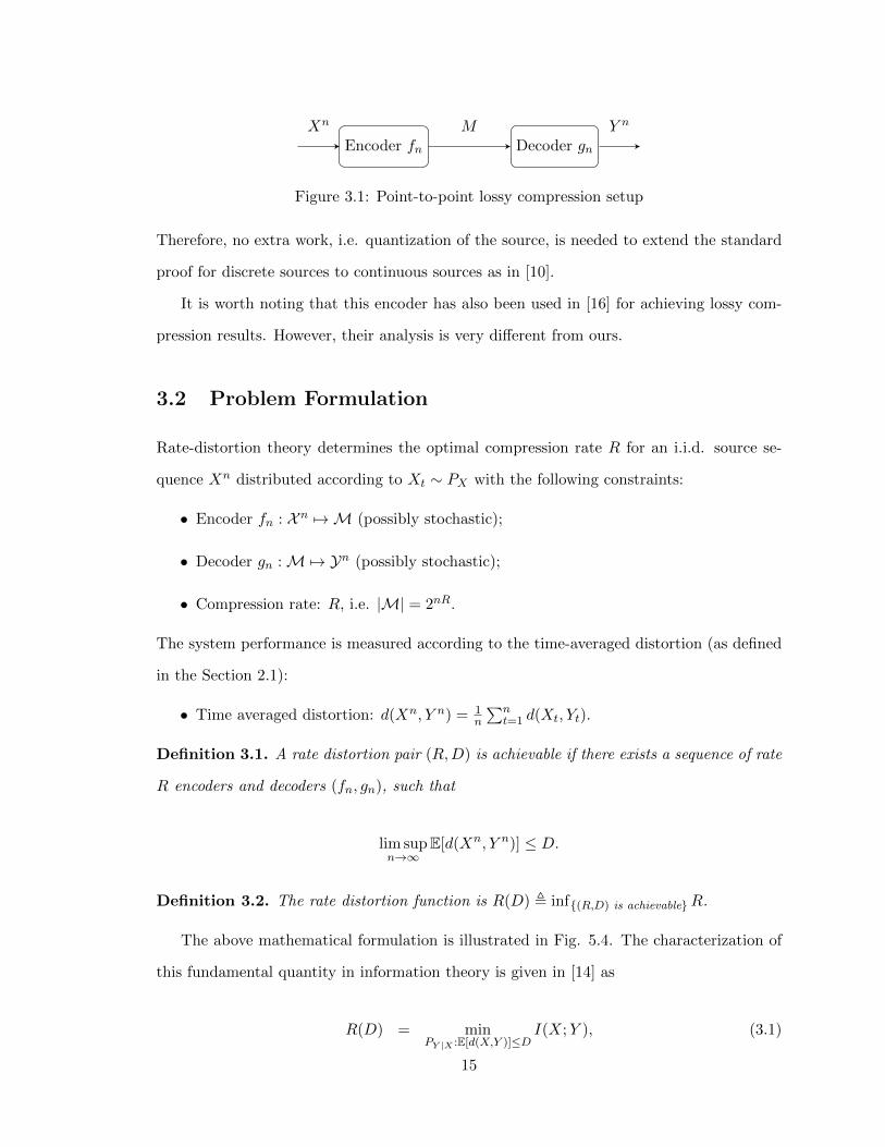
Encoder fn Decoder gn
Xn M Y n
Figure 3.1: Point-to-point lossy compression setup
Therefore, no extra work, i.e. quantization of the source, is needed to extend the standard
proof for discrete sources to continuous sources as in [10].
It is worth noting that this encoder has also been used in [16] for achieving lossy com-
pression results. However, their analysis is very different from ours.
3.2 Problem Formulation
Rate-distortion theory determines the optimal compression rate R for an i.i.d. source se-
quence Xn distributed according to Xt ∼ PX with the following constraints:
• Encoder fn : X n 7→ M (possibly stochastic);
• Decoder gn :M 7→ Yn (possibly stochastic);
• Compression rate: R, i.e. |M| = 2nR.
The system performance is measured according to the time-averaged distortion (as defined
in the Section 2.1):
• Time averaged distortion: d(Xn, Y n) = 1n
∑nt=1 d(Xt, Yt).
Definition 3.1. A rate distortion pair (R,D) is achievable if there exists a sequence of rate
R encoders and decoders (fn, gn), such that
lim supn→∞
E[d(Xn, Y n)] ≤ D.
Definition 3.2. The rate distortion function is R(D) , inf{(R,D) is achievable}R.
The above mathematical formulation is illustrated in Fig. 5.4. The characterization of
this fundamental quantity in information theory is given in [14] as
R(D) = minPY |X :E[d(X,Y )]≤D
I(X;Y ), (3.1)
15
where the mutual information is taken with respect to
PXY = PXPY |X . (3.2)
In other words, we are able to achieve distortion level D with any rate less than R(D) given
in the right hand side of (3.1).
The converse part of the proof for (3.1) can be found in standard textbooks such as [9]
[10], and is not presented here.
3.3 Achievability Using the Likelihood Encoder
To prove achievability, we will use the likelihood encoder and approximate the overall be-
havior of the system by a well-behaved distribution. The soft-covering lemma allows us to
claim that the approximating distribution matches the system.
Here we make an additional note on the notation. As mentioned in the Section 2.1,
P is reserved for denoting the system induced distribution. The single letter distributions
appearing in (3.1) are replaced with P in the following proof. The marginal and conditional
distributions derived from PXY are denoted as PX , P Y , PX|Y and P Y |X . Since PX =
PX , these can be used interchangeably. We use PXnY n to denote the product of an i.i.d.
distribution, i.e.
PXnY n =
n∏t=1
PXY , (3.3)
and similarly for the marginal and conditional distributions derived from PXY .
Let R > R(D), where R(D) is from the right hand side of (3.1). We prove that R
is achievable for distortion D. By the rate-distortion formula stated in (3.1), we can fix
P Y |X such that R > I(X;Y ) and E[d(X,Y )] < D, where the mutual information and the
expectation are taken with respect to PXY . We will use the likelihood encoder derived from
PXY and a random codebook {yn(m)} generated according to P Y to prove the result. The
decoder will simply reproduce yn(M) upon receiving the message M .
16
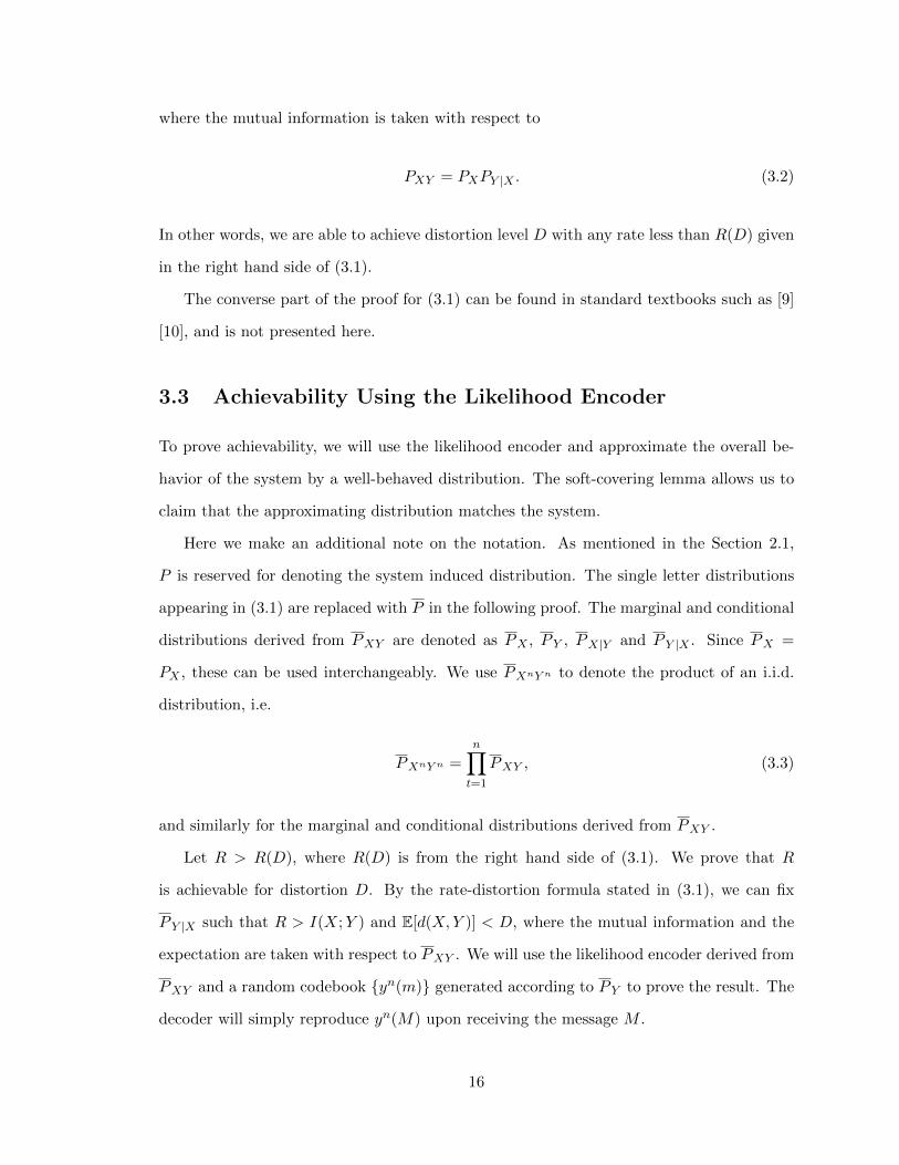
C(n) PX|Y
M Y n(M) Xn
Figure 3.2: Idealized distribution conditioned on a codebook C(n) with test channel PX|Y .
The distribution induced by the encoder and decoder is
PXnMY n(xn,m, yn)
= PXn(xn)PM |Xn(m|xn)PY n|M (yn|m) (3.4)
, PXn(xn)PLE(m|xn)PD(yn|m) (3.5)
where PLE is the likelihood encoder and PD is a codeword lookup decoder.
We now concisely restate the behavior of the encoder and decoder, as components of
the induced distribution.
Codebook generation: We independently generate 2nR sequences in Yn according to∏nt=1 P Y (yt) and index them by m ∈ [1 : 2nR]. We use C(n) to denote the random codebook.
Encoder: The encoder PLE(m|xn) is the likelihood encoder that chooses M stochasti-
cally with probability proportional to the likelihood function given by
L(m|xn) = PXn|Y n(xn|Y n(m)). (3.6)
Decoder: The decoder PD(yn|m) is a codeword lookup decoder that simply reproduces
Y n(m).
Analysis: We will consider two distributions for the analysis, the induced distribution
P and an approximating distribution Q, which is much easier to analyze. We will show
that P and Q are close in total variation (on average over the random codebook). Hence,
P achieves the performance of Q.
Design the approximating distribution Q via a uniform distribution over a random
codebook and a test channel PX|Y as shown in Fig. 3.2. We will refer to a distribution
of this structure as an idealized distribution. The joint distribution under the idealized
17
distribution Q shown in Fig. 3.2 can be written as
QXnMY n(xn,m, yn)
= QM (m)QY n|M (yn|m)QXn|M (xn|m) (3.7)
=1
2nR1{yn = Y n(m)}
n∏t=1
PX|Y (xt|Yt(m)) (3.8)
=1
2nR1{yn = Y n(m)}
n∏t=1
PX|Y (xt|yt). (3.9)
The idealized distribution Q has the following property: for any (xn, yn) ∈ X n × Yn,
EC(n) [QXnY n(xn, yn)]
= EC(n)
[1
2nR
∑m
1{yn = Y n(m)}
]n∏t=1
PX|Y (xt|yt) (3.10)
=1
2nR
∑m
EC(n) [1{yn = Y n(m)}]n∏t=1
PX|Y (xt|yt) (3.11)
=1
2nR
∑m
P Y n(yn)
n∏t=1
PX|Y (xt|yt) (3.12)
= PXnY n(xn, yn). (3.13)
This implies, in particular, that the distortion under the idealized distribution Q averaged
over the random codebook conveniently simplifies to EP [d(X,Y )]. That is,
EC(n) [EQ[d(Xn, Y n)]]
= EC(n)
[∑xn,yn
QXnY n(xn, yn)d(xn, yn)
](3.14)
=∑xn,yn
EC(n) [QXnY n(xn, yn)]d(xn, yn) (3.15)
=∑xn,yn
PXn,Y n(xn, yn)d(xn, yn) (3.16)
= EP [d(Xn, Y n)] (3.17)
= EP [d(X,Y )], (3.18)
18
where (3.16) follows from (3.13). It is worth emphasizing that although Q is very different
from the i.i.d. distribution on (Xn, Y n), it is exactly the i.i.d. distribution when averaged
over codebooks and thus achieves the same expected distortion.
Our motivation for using the likelihood encoder comes from this construction of Q.
Notice the following important facts:
QM |Xn(m|xn) = PLE(m|xn), (3.19)
and
QY n|M (yn|m) = PD(yn|m). (3.20)
Now invoking the basic soft-covering lemma (Lemma 2.1), since R > I(X;Y ), we have
EC(n)
[‖PXn −QXn‖TV
]≤ εn, (3.21)
where εn →n 0. This gives us
EC(n) [‖PXnY n −QXnY n‖TV ]
≤ EC(n) [‖PXnY nM −QXnY nM‖TV ] (3.22)
≤ εn, (3.23)
where (3.22) follows from Property 2.1(e) and (3.23) follows from (3.19),(3.20) and Property
2.1(d).
By Property 2.1(b),
|EP[d(Xn, Y n)]− EQ[d(Xn, Y n)]| ≤ dmax‖P−Q‖TV . (3.24)
19

Now we apply the random coding argument.
EC(n) [EP[d(Xn, Y n)]]
≤ EC(n) [EQ[d(Xn, Y n)]] + EC(n) [|EP[d(Xn, Y n)]− EQ[d(Xn, Y n)]|] (3.25)
≤ EP [d(X,Y )] + dmaxEC(n) [‖PXnY n −QXnY n‖TV ] (3.26)
≤ EP [d(X,Y )] + dmaxεn (3.27)
where (3.26) follows from (3.18) and (3.24); (3.27) follows from (3.23). Taking the limit on
the both sides gives:
lim supn→∞
EC(n) [EP[d(Xn, Y n)]] ≤ D, (3.28)
Therefore, there exists a codebook satisfying the requirement. �
3.4 Excess Distortion
3.4.1 Probability of Excess Distortion
The proof presented in the previous section is for the average distortion criterion, i.e.
lim sup→∞ E [d(Xn, Y n)] ≤ D. However, it is not hard to modify the proofs to show that
they also hold for excess distortion.
With the same setup as in Section 3.2, we change the average distortion requirement in
the definition of achievability (Definition 3.1) to excess distortion.
Definition 3.3. A rate distortion pair (R,D) is achievable under excess distortion if
there exists a sequence of rate R encoders and decoders (fn, gn), such that
P [d(Xn, Y n) > D]→n 0.
The corresponding rate-distortion function is still given by R(D) in (3.1).
For the excess distortion, we will use the exact same encoding/decoding scheme, along
with the same random codebook Cn, from Section 3.3. We make the following modifications.
20
We replace (3.14) to (3.18) with
EC(n) [PQ [d(Xn, Y n) > D]]
= EC(n)
[∑xn,yn
QXnY n(xn, yn)1{d(xn, yn) > D}
](3.29)
=∑xn,yn
EC(n) [QXnY n(xn, yn)]1{d(xn, yn) > D} (3.30)
=∑xn,yn
PXn,Y n(xn, yn)1{d(xn, yn) > D} (3.31)
= PP [d(Xn, Y n) > D], (3.32)
and replace (3.25) to (3.27) with
EC(n) [PP[d(Xn, Y n) > D]]
≤ EC(n) [PQ[d(Xn, Y n) > D]] + εn (3.33)
= PP [d(Xn, Y n) > D] + εn (3.34)
where the last step follows from (3.32). Therefore, there exists a codebook that satisfies the
requirement. �
3.4.2 Non-asymptotic Performance
Let the achievable rate-distortion region R be
R , {(R,D) : R > R(D)}.
For a fixed (R,D) ∈ R, we aim to minimize the probability of excess distortion, using a
random codebook and the likelihood encoder, over valid choices of P Y |X , and evaluate how
fast the excess distortion decays with blocklength n under the optimal P Y |X . Mathemati-
cally, we want to obtain
infPY |X
ECn [PP [d(Xn, Y n) > D]] , (3.35)
21
where the subscript P indicates probability taken with respect to the system induced dis-
tribution.
To evaluate how fast the probability of excess distortion approaches zero, note in (3.34)
that the first term is governed (approximately) by the gap D−EP [d(X,Y )] and the second
term is governed (approximately) by the the gap R−I(X;Y ), where the mutual information
is with respect to distribution PXY . To see this, observe that for any β > 0,
ε′n , PP [d(Xn, Y n) > D] (3.36)
= PP
[1
n
n∑t=1
d(Xt, Yt) > D
](3.37)
≤ infβ>0
[EP [2βd(X,Y )]
2βD
]n(3.38)
= exp
(−n log
(infβ>0
EP[2β(d(X,Y )−D)
])−1)
(3.39)
= exp(−nη(P Y |X)
)(3.40)
where (3.38) follows from the Chernoff bound and we have implicitly defined
η(P Y |X) , log
(infβ>0
EP[2β(d(X,Y )−D)
])−1
. (3.41)
An upper bound on the second term in (3.34) is given in [11], reproduced below:
εn ≤3
2exp
(−nγ(P Y |X)
), (3.42)
where
γ(P Y |X) , maxα≥1,α′≤2
α− 1
2α− α′(R− IP ,α(X;Y ) + (α′ − 1)(IP ,α(X;Y )− IP ,α′(X;Y ))
)(3.43)
IP ,α(X;Y ) ,1
α− 1log
(EP
[(PX,Y (X,Y )
PX(X)P Y (Y )
)α−1])
(3.44)
IP ,α′(X,Y ) ,1
α′ − 1log
EPX
√√√√EPY |X
[(PXY (X,Y )
PX(X)P Y (Y )
)α′−1]2
(3.45)
22
Both ε′n and εn decay exponentially with n. To obtain an upper bound on the excess
distortion given in (3.35), we now have a new optimization problem in the following form:
infPY |X
exp(−nη(P Y |X)
)+
3
2exp
(−nγ(P Y |X)
), (3.46)
where η(P Y |X) and γ(P Y |X) are defined in (3.41) and (3.43). Note that only choices of P Y |X
such that EP [d(X,Y )] < D and I(X;Y ) < R should be considered for the optimization, as
other choices render the bound degenerate.
We can relax (3.46) to obtain a simple upper bound on the excess distortion
PP [d(Xn, Y n) > D] given in the following theorem.
Theorem 3.1. The excess distortion PP [d(Xn, Y n) > D] using the likelihood encoder is
upper bounded by
infPY |X
5
2exp
(−nmin
{η(P Y |X
), γ(P Y |X
)}), (3.47)
where η(P Y |X) and γ(P Y |X) are given in (3.41) and (3.43), respectively.
Remark 1. Note that this bound does not achieve the exponent that we know to be optimal
[17, Theorem 9.5] for rate-distortion theory. It may very well be that the likelihood encoder
does not achieve the optimal exponent, though it may also be an artifact of our proof or the
bound for the soft-covering lemma.
3.4.3 Comparison with Random Binning Based Proof
The likelihood encoder proof technique is similar to the random binning based analysis
approach presented in [18] in many ways. In this section, we will compare the two schemes
along with their non-asymptotic behaviors.
We shall first provide a recap of the scheme for point-to-point lossy compression that
uses the so-called “output statistics of random binning” in the proof. Below we modify
the way it was originally presented in [18] to ease the comparison with the proof given in
Section 3.3.
23
The Proportional-Probability Encoder
We start by defining a source encoder that looks very similar in form to a likelihood encoder
defined in Section 2.4. Like any other source encoder, a proportional-probability encoder
receives a sequence x1, ..., xn and produces an index m ∈ [1 : 2nR].
A codebook is specified by a non-empty collection C of sequences yn ∈ Yn and indices
m(yn) assigned to each yn ∈ Yn. The codebook and a joint distribution PXY specify the
proportional-probability encoder.
Let G(m|xn) be the probability, as a result of passing xn through a memoryless channel
given by PY |X , of finding Y n in the collection C and retrieving the index m from the
codebook:
G(m|xn) , PPY n|Xn [Y n ∈ C,m(Y n) = m | Xn = xn] (3.48)
=∑yn∈C
PY n|Xn(yn|xn)1{m(yn) = m}, (3.49)
where PY n|Xn =∏nt=1 PY |X .
A proportional-probability encoder is a stochastic encoder that determines the message
index with probability proportional to G(m|xn), i.e.
PM |Xn(m|xn) =G(m|xn)∑
m′=[1:2nR] G(m′|xn)∝ G(m|xn). (3.50)
Scheme Using the Proportional-Probability Encoder
Before going into the achievability scheme, we first state a lemma that will be used in the
analysis.
Lemma 3.1 (Independence of random binning - Theorem 1 of [18]). Given a probability
mass function PXY , and each yn ∈ Yn is independently assigned to a bin index b ∈ [1 :
2nRb ] uniformly at random, where B(yn) denotes this random assignment. Define the joint
distribution
PXnY nB(xn, yn, b) ,n∏i=1
PXY (xi, yi)1{B(yn) = b}. (3.51)
24
If Rb < H(Y |X), then we have
EB[∥∥PXnB − PXnPUB
∥∥TV
]→n 0, (3.52)
where PUB is a uniform distribution on [1 : 2nRb ] and EB denotes expectation taken over the
random binning.
We now outline the encoding-decoding scheme based on the proportional-probability
encoder.
Fix a P Y |X that satisfies EP [d(X,Y )] < D and choose the rates R and R′ to satisfy
R′ < H(Y |X) and R + R′ > H(Y ), where the entropies are with respect to distribution
PXY .
Codebook generation: Each yn ∈ Yn is randomly and independently assigned to
the codebook C with probability 2−nR′. Then, independent of the construction of C, each
yn ∈ Yn is independently assigned uniformly at random to one of 2nR bins indexed by M .
Encoder: The encoder PPPE(m|xn) is the proportional-probability encoder with re-
spect to P . Specifically, the encoder chooses M stochastically according to (3.50), with G
based on P as follows:
G(m|xn) =∑yn∈C
P Y n|Xn(yn|xn)1{m(yn) = m}, (3.53)
where P Y n|Xn(yn|xn) =∏nt=1 P Y |X(yt|xt).
Decoder: The decoder PD(yn|m) selects a yn reconstruction that is in C and has index
m = M . There will usually be more than one such yn sequence, but rarely will there
be more than one “good” choice, due to the rates used. The decoder can choose that
most probable yn sequence or the unique typical sequence, etc. The proof in [18] uses a
“mismatch stochastic likelihood coder” (MSLC) [16] [19], and we will use their analysis for
the performance bound in Section 3.4.3.
Remark 2. Intuitively, a decoder can successfully decode the sequence intended by the
encoder since there are roughly 2nH(Y ) typical yn sequences, and the collection C together
25
with the binning index M provides high enough rate R′ + R > H(Y ) to uniquely identify
the sequence.
Analysis: The above scheme specifies a system induced distribution of the form
PXnMY n(xn,m, yn) = PXn(xn)PPPE(m|xn)PD(yn|m).
To analyze the above scheme, we start by replacing the codebook used for encoding
and decoding with a set of codebooks. Recall that the codebook consists of a collection
C and index assignments m(yn) that are both randomly constructed. Now consider a
set of 2nR′
collections {Cf}f∈[1:2nR′ ], indexed by f , created by assigning each yn sequence
in Yn randomly to exactly one collection equiprobably. From this we define a set of 2nR′
codebooks, one for each f , each one consisting of the collection Cf and the common message
index function m(yn). We use K to denote this set of random codebooks.
By this construction, the original random collection C in the codebook used by the
encoder and decoder is equivalent in probability to using the first codebook associated with
C1. It is also equivalent to using a random codebook in the set, which is a point we will
utilize shortly. The purpose of defining multiple codebooks is to facilitate general proof
tools associated with uniform random binning.
Here we summarize the proof given in [18]. In addition to the system induced random
variables, we introduce a random variable F which is uniformly distributed on the set
{1, . . . , 2nR′} and independent of Xn. The variable F selects the codebook to be used—
everything else about the encoding and decoding remains the same. We have noted that the
behavior and performance of this system with multiple codebooks is equivalent to that of
the actual encoding and decoding. Nevertheless, we will formalize this connection in (3.69).
For now, we refer to this new distribution that includes many codebooks as the pseudo
induced distribution P. According to P, there is a set of randomly generated codebooks,
and the one for use is selected by F .
26
The pseudo induced distribution can be expressed in the following form:
PFXnMY n(f, xn,m, yn)
= PF (f)PXn(xn)PPPE(m|xn, f)PD(yn|m, f). (3.54)
We reiterate that
PXnMY nd= PXnMY n|F=f , ∀f ∈ [1 : 2nR
′]. (3.55)
We now introduce one more random variable that never actually materialized during
the implementation. Let Y n be the reconstruction sequence intended by the encoder. The
encoding can be considered as a two step process. First, the encoder selects a Y n sequence
from Cf with probability proportional to that induced by passing xn through a memoryless
channel given by P Y |X . Next, the encoder looks up the message index m(Y n) and transmits
it as M .
Accordingly, we will replace the encoder in the pseudo induced distribution with the
two parts discussed:
PPPE(m|xn, f) =∑yn
PE1(yn|xn, f)PE2(m|yn). (3.56)
To analyze the expected distortion performance of the pseudo induced distribution P,
we introduce two approximating distributions Q(1) and Q(2).
Let us first define the distribution Q(1):
Q(1)
FXnY nMY n(f, xn, yn,m, yn)
, PXnY n(xn, yn)QF |Y n(f |yn)PE2(m|yn)PD(yn|m, f) (3.57)
where QF |Y n(f |yn) = 1{yn ∈ Cf}. In words, Q(1) is constructed from an i.i.d. distribution
according to P on (Xn, Y n), two random binnings F and M , as specified by the construction
of the set of codebooks K, and a decoding of Y n from the random binnings.
27
Now we arrive at the reason for using the proportional-probability encoder. Part 1 of
the encoder that selects the Y n sequences is precisely the conditional probability specified
by Q(1):
Q(1)
Y n|XnF(yn|xn, f) = PE1(yn|xn, f).
Therefore, the only difference between the pseudo induced distribution P and Q(1) is the
conditional distribution of F given Xn, which should be independent and uniform according
to P. This is where Lemma 3.1 plays a role.
Applying Lemma 3.1 by identifying F as the uniform binning of Y n, since R′ < H(Y |X)
under distribution PXY , we obtain
EK[∥∥∥Q(1)
XnF − PXnF
∥∥∥TV
]≤ ε(rb)n →n 0. (3.58)
Using Property 2.1(d), we have
EK[∥∥∥PFXnY nMY n −Q
(1)
FXnY nMY n
∥∥∥TV
]≤ ε(rb)n . (3.59)
The next approximating distribution we define is Q(2):
Q(2)
FXnY nMY n(f, xn, yn,m, yn) , Q
(1)
FXnY nM(f, xn, yn,m)1{yn = yn}. (3.60)
Recall from Remark 2, decoding Y n will succeed with high probability if the total rate
of the binnings is above the entropy rate of the sequence that was binned. This is well
known from the Slepian-Wolf coding result [20] [21]. Therefore, since the total binning rate
R + R′ > H(Y ) under distribution P Y , according to the definition of total variation, we
obtain
EK[∥∥∥Q(1)
Y nY n−Q
(2)
Y nY n
∥∥∥TV
]≤ ε(sw)
n →n 0, (3.61)
where ε(sw)n is the decoding error.
28
Again by Property 2.1(d), we have
EK[∥∥∥Q(1)
FXnY nMY n−Q
(2)
FXnY nMY n
∥∥∥TV
]≤ ε(sw)
n . (3.62)
Combining (3.59) and (3.62) using the triangle inequality, we obtain
EK[∥∥∥PFXnY nMY n −Q
(2)
FXnY nMY n
∥∥∥TV
]≤ ε(rb)n + ε(sw)
n . (3.63)
Note that the distortion under any realization of Q(2), regardless of the codebook, is
EQ(2) [d(Xn, Y n)] = EQ(2) [d(Xn, Y n)] (3.64)
= EP [d(X,Y )]. (3.65)
Applying Property 2.1(b), we can obtain
EK[EP[d(Xn, Y n)]
]≤ EP [d(X,Y )] + dmax(ε(rb)n + ε(sw)
n ). (3.66)
Furthermore, by symmetry and the law of total expectation, we have
EK[EP[d(Xn, Y n)]
]= EF
[EK[EP[d(Xn, Y n)] | F
]](3.67)
= EK[EP[d(Xn, Y n)] | F = 1
](3.68)
= EK [EP[d(Xn, Y n)]] , (3.69)
where the last equality comes from the observation in (3.55).
Finally, applying the random coding argument, there exists a code that gives
EP [d(Xn, Y n)] ≤ EP [d(X,Y )] + dmax
(ε(rb)n + ε(sw)
n
),
which is less than D for n large enough.
29
Comparing the Likelihood Encoder with Proportional-Probability Encoder
Let us now compare the achievability proofs using the likelihood encoder approach and the
proportional-probability encoder (random binning based) approach for the point-to-point
rate distortion function.
We first notice that the error term in the likelihood encoder approach only arises from
the soft-covering lemma, while the error terms in the proportional-probability approach
come from two places, random binning and MSLC decoding.
Next, we will provide a non-asymptotic comparison between the two approaches with
respect to excess distortion.
Some asymptotic analysis was given in [19] on channel coding with random binning.
We can extend this to give non-asymptotic bounds for source coding problems also. Using
Theorems 1 and 2 from [19], we can obtain the following theorem.
Theorem 3.2. The excess distortion PP [d(Xn, Y n) > D] using the proportional-probability
encoder is upper bounded by
infPY |X
{exp
(−nη(P Y |X)
)+ σn(P Y |X)
}(3.70)
where
σn(P Y |X) = infR′∈(H(Y )−R,H(Y |X))
{An +Bn} (3.71)
and
An = infδ∈(0,H(Y |X)−R′)
{PP[− logP Y n|Xn(Y n|Xn) ≤ n(R′ + δ)
]+
1√2
2−nδ2
}(3.72)
Bn = infτ>0
{PP[n(R+R′)− h(Y n) ≤ nτ
]+ 3× 2−nτ
}. (3.73)
We can further bound the quantities in An and Bn in Theorem 3.2 by the Chernoff
inequality following the steps (3.37) through (3.40) and obtain the following exponential
30
forms:
PP[− logP Y n|Xn(Y n|Xn) ≤ n(R′ + δ)
]≤ inf
β1>0
exp
−n log
(EP
[2β1
(R′+δ−log 1
PY |X (Y |X)
)])−1 , (3.74)
PP[n(R+R′)− h(Y n) ≤ nτ
]≤ inf
β2>0
exp
−n log
(EP
[2β2
(log 1
PY (Y )−R−R′+τ
)])−1 . (3.75)
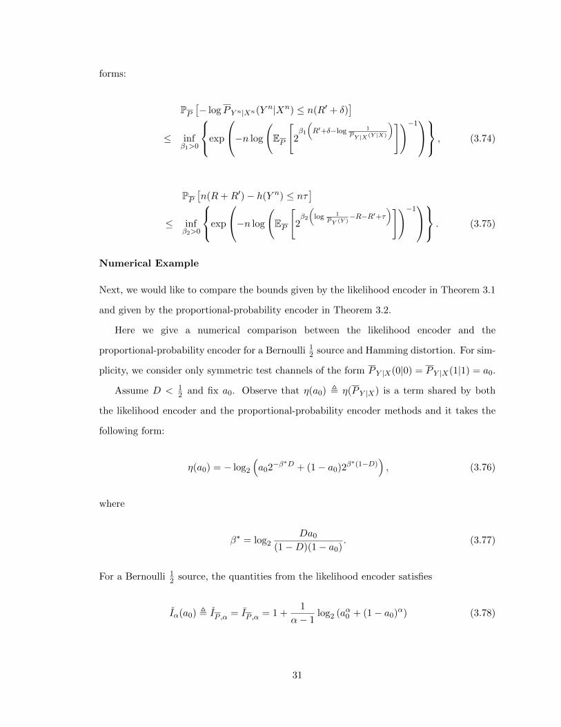
Numerical Example
Next, we would like to compare the bounds given by the likelihood encoder in Theorem 3.1
and given by the proportional-probability encoder in Theorem 3.2.
Here we give a numerical comparison between the likelihood encoder and the
proportional-probability encoder for a Bernoulli 12 source and Hamming distortion. For sim-
plicity, we consider only symmetric test channels of the form P Y |X(0|0) = P Y |X(1|1) = a0.
Assume D < 12 and fix a0. Observe that η(a0) , η(P Y |X) is a term shared by both
the likelihood encoder and the proportional-probability encoder methods and it takes the
following form:
η(a0) = − log2
(a02−β
∗D + (1− a0)2β∗(1−D)
), (3.76)
where
β∗ = log2
Da0
(1−D)(1− a0). (3.77)
For a Bernoulli 12 source, the quantities from the likelihood encoder satisfies
Iα(a0) , IP ,α = IP ,α = 1 +1
α− 1log2 (aα0 + (1− a0)α) (3.78)
31
γ(a0) = maxα≥1,α′≤2
α− 1
2α− α′
(R− 1 +
α′ − 2
α− 1log2(aα0 + (1− a0)α)− log2(aα
′0 + (1− a0)α
′)
).(3.79)
Observe that the first term in Bn given in (3.73) is deterministic; therefore, we can choose
τ∗ = R+R′ − 1. (3.80)
The optimum β1 in (3.74) is given by
β∗1 =
[log a0
1−a0
(−R
′ + δ + log2(1− a0)
R′ + δ + log2(a0)
)− 1
]+
. (3.81)
Consequently, the exponent of the first term of An is given by
A1n(R′, δ, a0) , − log2
(a02β
∗1 (R′+δ+log2(a0)) + (1− a0)2β
∗1 (R′+δ+log2(1−a0))
). (3.82)
Let us define
λ(a0) , maxR′,δ
(R+R′ − 1,
δ
2, A1(R′, δ, a0)
),
where the domains of R′ and δ are omitted.
To summarize, for the likelihood encoder, we still need to optimize over α and α′, and
for the proportional-probability encoder, we need to optimize over R′ and δ. Finally, for
both, we optimize over a0. The derived error exponent bounds for the likelihood encoder
and the proportional-probability encoder are given by the following, respectively:
Error exponent for the LE = maxa0
min(η(a0), γ(a0)) (3.83)
Error exponent for the PPE = maxa0
min(η(a0), λ(a0)). (3.84)
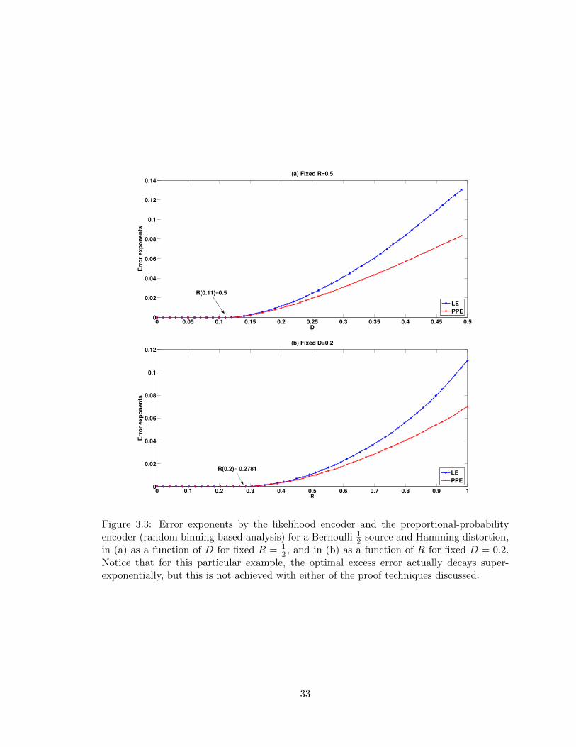
Comparisons of the error exponents given in (3.83) and (3.84) are shown in Fig. 3.3,
plotted as functions of D and R. The numerical comparisons show that the likelihood
encoder has a better error exponent than the proportional-probability encoder, at least
according to these derived upper bounds on the error.
32
0 0.05 0.1 0.15 0.2 0.25 0.3 0.35 0.4 0.45 0.50
0.02
0.04
0.06
0.08
0.1
0.12
0.14
D
Err
or
ex
po
ne
nts
(a) Fixed R=0.5
LE
PPE
R(0.11)≈0.5
0 0.1 0.2 0.3 0.4 0.5 0.6 0.7 0.8 0.9 10
0.02
0.04
0.06
0.08
0.1
0.12
R
Err
or
ex
po
ne
nts
(b) Fixed D=0.2
LE
PPE
R(0.2)≈ 0.2781
Figure 3.3: Error exponents by the likelihood encoder and the proportional-probabilityencoder (random binning based analysis) for a Bernoulli 1
2 source and Hamming distortion,in (a) as a function of D for fixed R = 1
2 , and in (b) as a function of R for fixed D = 0.2.Notice that for this particular example, the optimal excess error actually decays super-exponentially, but this is not achieved with either of the proof techniques discussed.
33
3.5 A Non-Asymptotic Analysis Using Jensen’s Inequality
The excess distortion can be examined using the same type of analysis as the “one shot
achievability” for channel coding [16]. The key step again uses Jensen’s inequality and it
gives us an upper bound on the excess distortion.
Here, instead of looking at an i.i.d. source sequence, we perform the analysis on a general
source with distribution given as PX . Fix P Y |X and denote PXY = PXP Y |X .
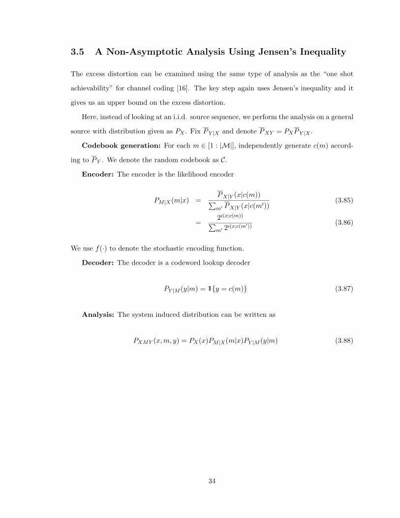
Codebook generation: For each m ∈ [1 : |M|], independently generate c(m) accord-
ing to P Y . We denote the random codebook as C.
Encoder: The encoder is the likelihood encoder
PM |X(m|x) =PX|Y (x|c(m))∑m′ PX|Y (x|c(m′))
(3.85)
=2ı(x;c(m))∑m′ 2
ı(x;c(m′))(3.86)
We use f(·) to denote the stochastic encoding function.
Decoder: The decoder is a codeword lookup decoder
PY |M (y|m) = 1{y = c(m)} (3.87)
Analysis: The system induced distribution can be written as
PXMY (x,m, y) = PX(x)PM |X(m|x)PY |M (y|m) (3.88)
34
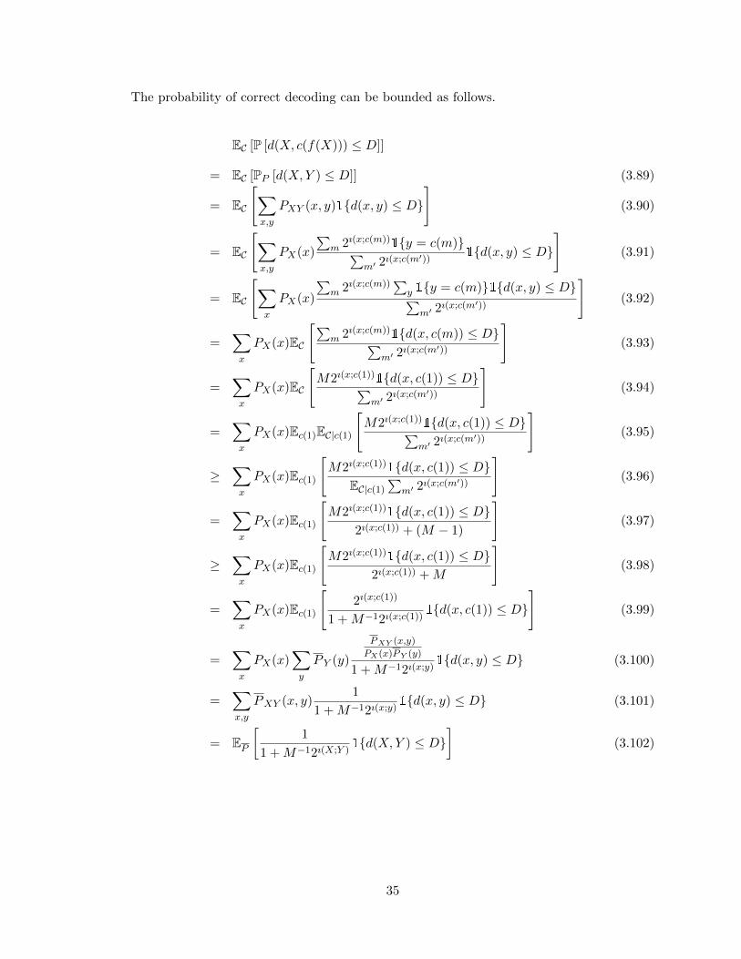
The probability of correct decoding can be bounded as follows.
EC [P [d(X, c(f(X))) ≤ D]]
= EC [PP [d(X,Y ) ≤ D]] (3.89)
= EC
[∑x,y
PXY (x, y)1{d(x, y) ≤ D}
](3.90)
= EC
[∑x,y
PX(x)
∑m 2ı(x;c(m))
1{y = c(m)}∑m′ 2
ı(x;c(m′))1{d(x, y) ≤ D}
](3.91)
= EC
[∑x
PX(x)
∑m 2ı(x;c(m))
∑y 1{y = c(m)}1{d(x, y) ≤ D}∑m′ 2
ı(x;c(m′))
](3.92)
=∑x
PX(x)EC
[∑m 2ı(x;c(m))
1{d(x, c(m)) ≤ D}∑m′ 2
ı(x;c(m′))
](3.93)
=∑x
PX(x)EC
[M2ı(x;c(1))
1{d(x, c(1)) ≤ D}∑m′ 2
ı(x;c(m′))
](3.94)
=∑x
PX(x)Ec(1)EC|c(1)
[M2ı(x;c(1))
1{d(x, c(1)) ≤ D}∑m′ 2
ı(x;c(m′))
](3.95)
≥∑x
PX(x)Ec(1)
[M2ı(x;c(1))
1{d(x, c(1)) ≤ D}EC|c(1)
∑m′ 2
ı(x;c(m′))
](3.96)
=∑x
PX(x)Ec(1)
[M2ı(x;c(1))
1{d(x, c(1)) ≤ D}2ı(x;c(1)) + (M − 1)
](3.97)
≥∑x
PX(x)Ec(1)
[M2ı(x;c(1))
1{d(x, c(1)) ≤ D}2ı(x;c(1)) +M
](3.98)
=∑x
PX(x)Ec(1)
[2ı(x;c(1))
1 +M−12ı(x;c(1))1{d(x, c(1)) ≤ D}
](3.99)
=∑x
PX(x)∑y
P Y (y)
PXY (x,y)
PX(x)PY (y)
1 +M−12ı(x;y)1{d(x, y) ≤ D} (3.100)
=∑x,y
PXY (x, y)1
1 +M−12ı(x;y)1{d(x, y) ≤ D} (3.101)
= EP
[1
1 +M−12ı(X;Y )1{d(X,Y ) ≤ D}
](3.102)
35
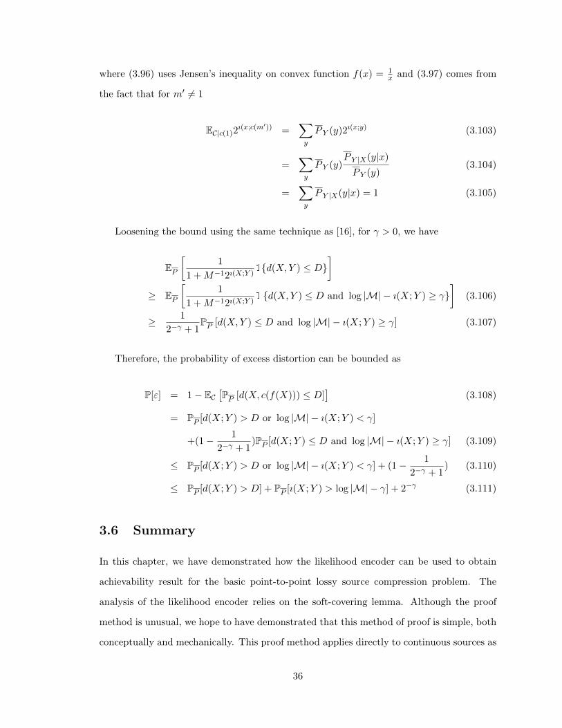
where (3.96) uses Jensen’s inequality on convex function f(x) = 1x and (3.97) comes from
the fact that for m′ 6= 1
EC|c(1)2ı(x;c(m′)) =
∑y
P Y (y)2ı(x;y) (3.103)
=∑y
P Y (y)P Y |X(y|x)
P Y (y)(3.104)
=∑y
P Y |X(y|x) = 1 (3.105)
Loosening the bound using the same technique as [16], for γ > 0, we have
EP
[1
1 +M−12ı(X;Y )1{d(X,Y ) ≤ D}
]≥ EP
[1
1 +M−12ı(X;Y )1 {d(X,Y ) ≤ D and log |M| − ı(X;Y ) ≥ γ}
](3.106)
≥ 1
2−γ + 1PP [d(X,Y ) ≤ D and log |M| − ı(X;Y ) ≥ γ] (3.107)
Therefore, the probability of excess distortion can be bounded as
P[ε] = 1− EC[PP [d(X, c(f(X))) ≤ D]
](3.108)
= PP [d(X;Y ) > D or log |M| − ı(X;Y ) < γ]
+(1− 1
2−γ + 1)PP [d(X;Y ) ≤ D and log |M| − ı(X;Y ) ≥ γ] (3.109)
≤ PP [d(X;Y ) > D or log |M| − ı(X;Y ) < γ] + (1− 1
2−γ + 1) (3.110)
≤ PP [d(X;Y ) > D] + PP [ı(X;Y ) > log |M| − γ] + 2−γ (3.111)
3.6 Summary
In this chapter, we have demonstrated how the likelihood encoder can be used to obtain
achievability result for the basic point-to-point lossy source compression problem. The
analysis of the likelihood encoder relies on the soft-covering lemma. Although the proof
method is unusual, we hope to have demonstrated that this method of proof is simple, both
conceptually and mechanically. This proof method applies directly to continuous sources as
36

well with no need for additional arguments, because the soft-covering lemma is not restricted
to discrete sources.
A parallel comparison of the non-asymptotic performance of the likelihood encoder and
the “proportional-probability encoder” has been provided along with a numerical exam-
ple. In this example, the likelihood encoder achieves better error exponents than does the
proportional probability encoder.
37

Chapter 4
Multiuser Lossy Compression
4.1 Introduction
In this chapter, we propose using a likelihood encoder to achieve classical source coding
results such as the Wyner-Ziv rate-distortion function and Berger-Tung inner bound [22]
[23]. In the standard proofs using the joint asymptotic equipartition principle (J-AEP), the
distortion analysis involves bounding several “error” events which may come from either
encoding or decoding. In the cases where there are multiple information sources, such as
side information at the decoder, intricacies arise, such as the need for a Markov lemma [9]
and [10]. These subtleties also lead to error-prone proofs involving the analysis of error
caused by random binning, which have been pointed out in several existing works [8] [24].
Since the analysis using the soft-covering lemma is not limited to discrete alphabets,
no extra work, i.e. quantization of the source, is needed to extend the standard proof for
discrete sources to continuous sources as in [10]. This advantage becomes more desirable for
the multi-terminal case, since generalization of the type-covering lemma and the Markov
lemma to continuous alphabets is non-trivial. Strong versions of the Markov lemma on
finite alphabets that can prove the Berger-Tung inner bound can be found in [10] and [25].
However, generalization to the continuous alphabets is still an ongoing research topic. Some
work, such as [26], has been dedicated to making this transition, yet is not strong enough
to be applied to the Berger-Tung case.
38
4.2 Approximation Lemma
Lemma 4.1. For a distribution PUV X and 0 < ε < 1, if P[U 6= V ] ≤ ε, then
‖PUX − PV X‖TV ≤ ε.
Proof. By definition,
‖PUX − PV X‖TV = supA∈F{P[(U,X) ∈ A]− P[(V,X) ∈ A]} .
Since for every A ∈ F
P[(U,X) ∈ A]− P[(V,X) ∈ A]
≤ P[(U,X) ∈ A]− P[(V,X) ∈ A, (U,X) ∈ A] (4.1)
= P[(U,X) ∈ A, (V,X) 6= A] (4.2)
≤ P[U 6= V ] (4.3)
≤ ε, (4.4)
we have
supA∈F{P[(U,X) ∈ A]− P[(V,X) ∈ A]} ≤ ε.
4.3 The Wyner-Ziv Setting
In this section, we will use the mechanism that was established in Section 3.3 and build upon
it to solve a more complicated problem. The Wyner-Ziv problem, that is, the rate-distortion
function with side information at the decoder, was solved in [27].
4.3.1 Problem Formulation
The source and side information pair (Xn, Zn) is distributed i.i.d. according to (Xt, Zt) ∼
PXZ . The system has the following constraints:
39
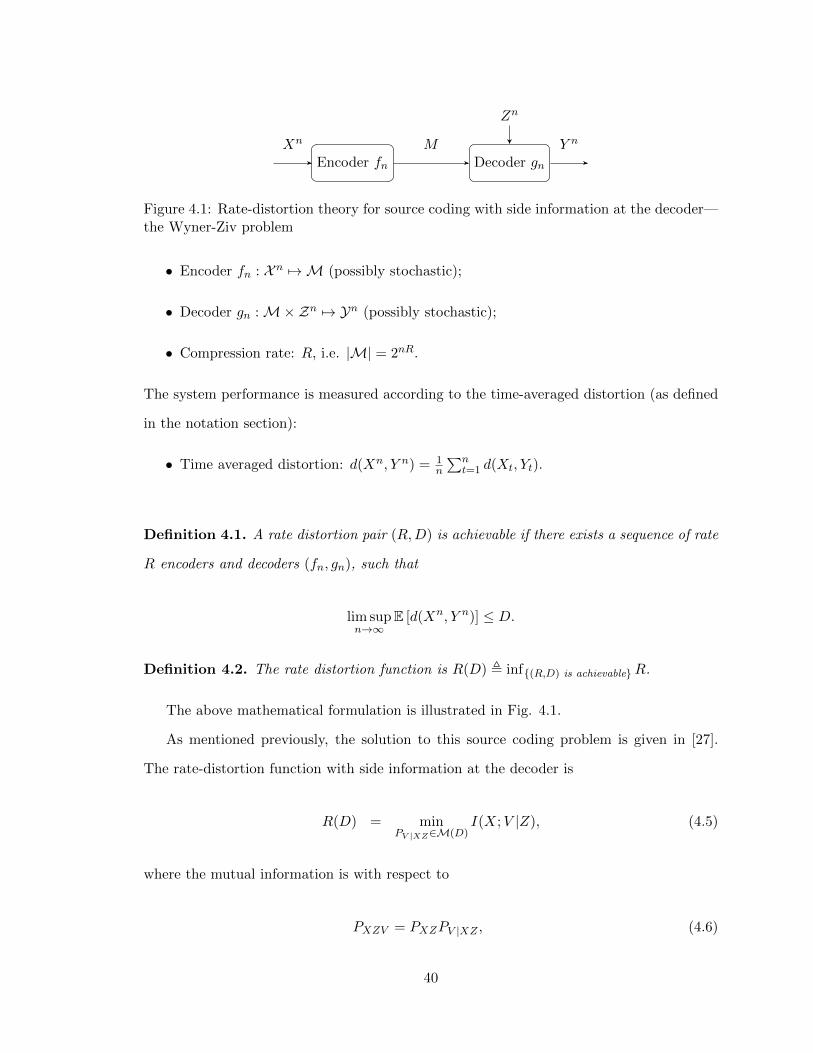
Encoder fn Decoder gn
Xn M Y n
Zn
Figure 4.1: Rate-distortion theory for source coding with side information at the decoder—the Wyner-Ziv problem
• Encoder fn : X n 7→ M (possibly stochastic);
• Decoder gn :M×Zn 7→ Yn (possibly stochastic);
• Compression rate: R, i.e. |M| = 2nR.
The system performance is measured according to the time-averaged distortion (as defined
in the notation section):
• Time averaged distortion: d(Xn, Y n) = 1n
∑nt=1 d(Xt, Yt).
Definition 4.1. A rate distortion pair (R,D) is achievable if there exists a sequence of rate
R encoders and decoders (fn, gn), such that
lim supn→∞
E [d(Xn, Y n)] ≤ D.
Definition 4.2. The rate distortion function is R(D) , inf{(R,D) is achievable}R.
The above mathematical formulation is illustrated in Fig. 4.1.
As mentioned previously, the solution to this source coding problem is given in [27].
The rate-distortion function with side information at the decoder is
R(D) = minPV |XZ∈M(D)
I(X;V |Z), (4.5)
where the mutual information is with respect to
PXZV = PXZPV |XZ , (4.6)
40
and
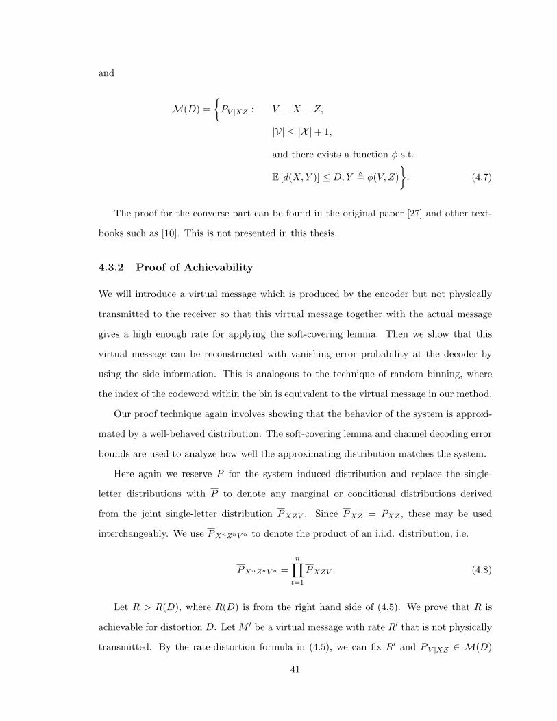
M(D) =
{PV |XZ : V −X − Z,
|V| ≤ |X |+ 1,
and there exists a function φ s.t.
E [d(X,Y )] ≤ D,Y , φ(V,Z)
}. (4.7)
The proof for the converse part can be found in the original paper [27] and other text-
books such as [10]. This is not presented in this thesis.
4.3.2 Proof of Achievability
We will introduce a virtual message which is produced by the encoder but not physically
transmitted to the receiver so that this virtual message together with the actual message
gives a high enough rate for applying the soft-covering lemma. Then we show that this
virtual message can be reconstructed with vanishing error probability at the decoder by
using the side information. This is analogous to the technique of random binning, where
the index of the codeword within the bin is equivalent to the virtual message in our method.
Our proof technique again involves showing that the behavior of the system is approxi-
mated by a well-behaved distribution. The soft-covering lemma and channel decoding error
bounds are used to analyze how well the approximating distribution matches the system.
Here again we reserve P for the system induced distribution and replace the single-
letter distributions with P to denote any marginal or conditional distributions derived
from the joint single-letter distribution PXZV . Since PXZ = PXZ , these may be used
interchangeably. We use PXnZnV n to denote the product of an i.i.d. distribution, i.e.
PXnZnV n =
n∏t=1
PXZV . (4.8)
Let R > R(D), where R(D) is from the right hand side of (4.5). We prove that R is
achievable for distortion D. Let M ′ be a virtual message with rate R′ that is not physically
transmitted. By the rate-distortion formula in (4.5), we can fix R′ and P V |XZ ∈ M(D)
41
(P V |XZ = P V |X) such that R+R′ > I(X;V ) and R′ < I(V ;Z), and there exists a function
φ(·, ·) yielding Y = φ(V,Z) and E [d(X,Y )] ≤ D. We will use the likelihood encoder derived
from PXV and a random codebook {vn(m,m′)} generated according to P V to prove the
result. The decoder will first use the transmitted message M and the side information Zn
to decode M ′ as M ′ and reproduce vn(M, M ′). Then the reconstruction Y n is produced as
a symbol-by-symbol application of φ(·, ·) to Zn and V n.
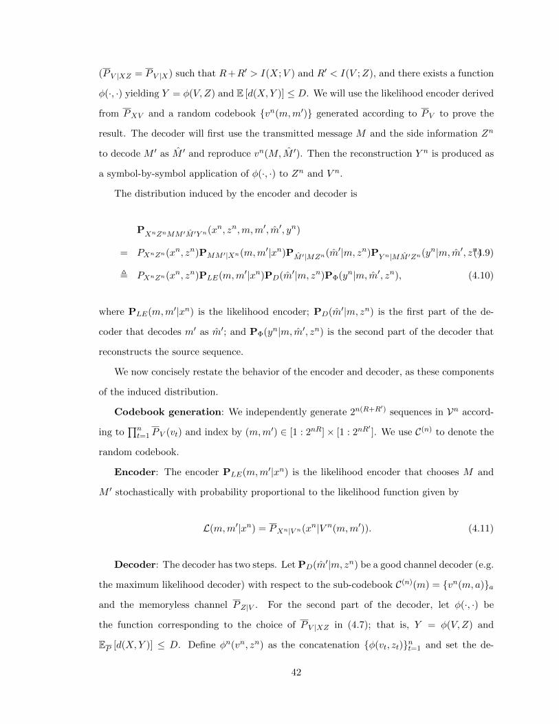
The distribution induced by the encoder and decoder is
PXnZnMM ′M ′Y n(xn, zn,m,m′, m′, yn)
= PXnZn(xn, zn)PMM ′|Xn(m,m′|xn)PM ′|MZn(m′|m, zn)PY n|MM ′Zn(yn|m, m′, zn)(4.9)
, PXnZn(xn, zn)PLE(m,m′|xn)PD(m′|m, zn)PΦ(yn|m, m′, zn), (4.10)
where PLE(m,m′|xn) is the likelihood encoder; PD(m′|m, zn) is the first part of the de-
coder that decodes m′ as m′; and PΦ(yn|m, m′, zn) is the second part of the decoder that
reconstructs the source sequence.
We now concisely restate the behavior of the encoder and decoder, as these components
of the induced distribution.
Codebook generation: We independently generate 2n(R+R′) sequences in Vn accord-
ing to∏nt=1 P V (vt) and index by (m,m′) ∈ [1 : 2nR]× [1 : 2nR
′]. We use C(n) to denote the
random codebook.
Encoder: The encoder PLE(m,m′|xn) is the likelihood encoder that chooses M and
M ′ stochastically with probability proportional to the likelihood function given by
L(m,m′|xn) = PXn|V n(xn|V n(m,m′)). (4.11)
Decoder: The decoder has two steps. Let PD(m′|m, zn) be a good channel decoder (e.g.
the maximum likelihood decoder) with respect to the sub-codebook C(n)(m) = {vn(m, a)}a
and the memoryless channel PZ|V . For the second part of the decoder, let φ(·, ·) be
the function corresponding to the choice of P V |XZ in (4.7); that is, Y = φ(V,Z) and
EP [d(X,Y )] ≤ D. Define φn(vn, zn) as the concatenation {φ(vt, zt)}nt=1 and set the de-
42
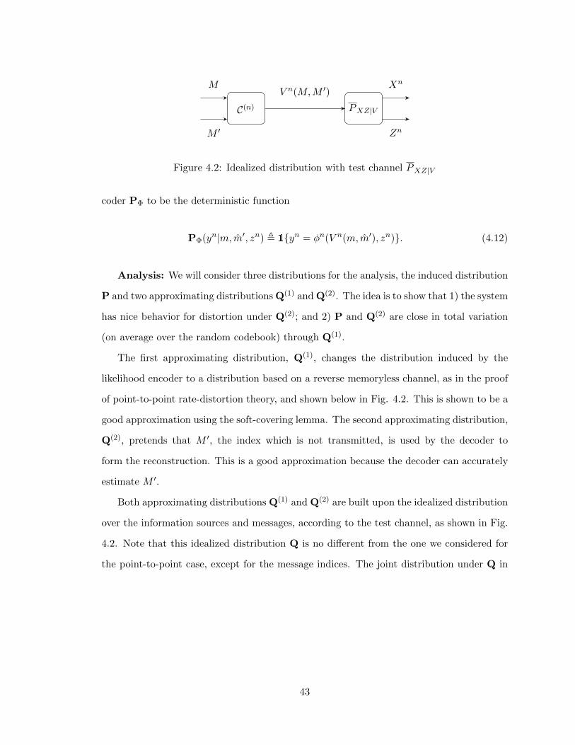
C(n) PXZ|V
M
M ′
V n(M,M ′)Xn
Zn
Figure 4.2: Idealized distribution with test channel PXZ|V
coder PΦ to be the deterministic function
PΦ(yn|m, m′, zn) , 1{yn = φn(V n(m, m′), zn)}. (4.12)
Analysis: We will consider three distributions for the analysis, the induced distribution
P and two approximating distributions Q(1) and Q(2). The idea is to show that 1) the system
has nice behavior for distortion under Q(2); and 2) P and Q(2) are close in total variation
(on average over the random codebook) through Q(1).
The first approximating distribution, Q(1), changes the distribution induced by the
likelihood encoder to a distribution based on a reverse memoryless channel, as in the proof
of point-to-point rate-distortion theory, and shown below in Fig. 4.2. This is shown to be a
good approximation using the soft-covering lemma. The second approximating distribution,
Q(2), pretends that M ′, the index which is not transmitted, is used by the decoder to
form the reconstruction. This is a good approximation because the decoder can accurately
estimate M ′.
Both approximating distributions Q(1) and Q(2) are built upon the idealized distribution
over the information sources and messages, according to the test channel, as shown in Fig.
4.2. Note that this idealized distribution Q is no different from the one we considered for
the point-to-point case, except for the message indices. The joint distribution under Q in
43
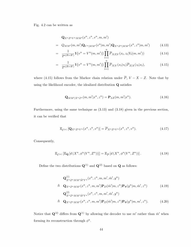
Fig. 4.2 can be written as
QXnZnV nMM ′(xn, zn, vn,m,m′)
= QMM ′(m,m′)QV n|MM ′(v
n|m,m′)QXnZn|MM ′(xn, zn|m,m′) (4.13)
=1
2n(R+R′)1{vn = V n(m,m′)}
n∏t=1
PXZ|V (xt, zt|Vt(m,m′)) (4.14)
=1
2n(R+R′)1{vn = V n(m,m′)}
n∏t=1
PX|V (xt|vt)PZ|X(zt|xt), (4.15)
where (4.15) follows from the Markov chain relation under P , V − X − Z. Note that by
using the likelihood encoder, the idealized distribution Q satisfies
QMM ′|XnZn(m,m′|xn, zn) = PLE(m,m′|xn). (4.16)
Furthermore, using the same technique as (3.13) and (3.18) given in the previous section,
it can be verified that
EC(n) [QXnZnV n(xn, zn, vn)] = PXnZnV n(xn, zn, vn). (4.17)
Consequently,
EC(n) [EQ [d (Xn, φn(V n, Zn))]] = EP [d (Xn, φn(V n, Zn))] . (4.18)
Define the two distributions Q(1) and Q(2) based on Q as follows:
Q(1)
XnZnMM ′M ′Y n(xn, zn,m,m′, m′, yn)
, QXnZnMM ′(xn, zn,m,m′)PD(m′|m, zn)PΦ(yn|m, m′, zn) (4.19)
Q(2)
XnZnMM ′M ′Y n(xn, zn,m,m′, m′, yn)
, QXnZnMM ′(xn, zn,m,m′)PD(m′|m, zn)PΦ(yn|m,m′, zn). (4.20)
Notice that Q(2) differs from Q(1) by allowing the decoder to use m′ rather than m′ when
forming its reconstruction through φn.
44
Therefore, on account of (4.17),
EC(n)
[Q
(2)XnZnY n(xn, zn, yn)
]= PXnZnY n(xn, zn, yn). (4.21)
Now applying the basic soft-covering lemma 2.1, since R+R′ > I(Z,X;V ) = I(X;V ),
we have
EC(n)
[‖PXnZn −QXnZn‖TV
]≤ εn →n 0. (4.22)
And with (4.10), (4.16), (4.19) and Property 2.1(d), we obtain
EC(n)
[‖PXnZnMM ′M ′Y n −Q
(1)
XnZnMM ′M ′Y n‖TV
]= EC(n)
[‖PXnZn −QXnZn‖TV
](4.23)
≤ εn. (4.24)
Since by definition Q(1)
XnZnMM ′M ′= Q
(2)
XnZnMM ′M ′,
PQ(1) [M ′ 6= M ′] = PQ(2) [M ′ 6= M ′]. (4.25)
Also, since R′ < I(V ;Z), the codebook is randomly generated, and M ′ is uniformly dis-
tributed under Q, it is well known that the maximum likelihood decoder PD (as well as
a variety of other decoders) will drive the error probability to zero as n goes to infinity.
This can be seen from Fig. 4.2, by identifying, for fixed M , that M ′ is the message to be
transmitted over the memoryless channel PZ|V . Specifically,
EC(n)
[PQ(1) [M ′ 6= M ′]
]≤ δn →n 0. (4.26)
Applying Lemma 4.1, we obtain
EC(n)
[‖Q(1)
XnZnMM ′−Q
(2)XnZnMM ′‖TV
]≤ EC(n)
[PQ(1) [M ′ 6= M ′]
]≤ δn. (4.27)
45
Thus by Property 2.1(d) and definitions (4.19) and (4.20),
EC(n)
[‖Q(1)
XnZnMM ′Y n−Q
(2)XnZnMM ′Y n‖TV
]≤ δn. (4.28)
Combining (4.24) and (4.28) and using Property 2.1(c) and 2.1(e), we have
EC(n)
[‖PXnY n −Q
(2)XnY n‖TV
]≤ εn + δn (4.29)
where εn and δn are the error terms introduced from the soft-covering lemma and channel
coding, respectively.
Repeating the same steps as (3.25) through (3.27) on P, Q(2), and P , we obtain
lim supn→∞
EC(n) [EP[d(Xn, Y n)]] ≤ lim supn→∞
{EP [d(X,Y )] + dmax(εn + δn)
}≤ D. (4.30)
Therefore, there exists a codebook satisfying the requirement. �
4.4 The Berger-Tung Inner Bound
In this section, we will demonstrate the use of the likelihood encoder via an alternative
proof for achieving the Berger-Tung inner bound for the problem of multi-terminal source
coding. Notice that no Markov lemma is needed in this proof. Similar to the single-user
case, the key is to identify an auxiliary distribution that has nice properties and show that
the system-induced distribution and the auxiliary distribution we choose are close in total
variation.
4.4.1 Problem Formulation
We now consider a pair of correlated sources (X1n, X2
n), distributed i.i.d. according to
(X1t, X2t) ∼ PX1X2 , independent encoders, and a joint decoder, satisfying the following
constraints:
• Encoder 1 f1n : X1n 7→ M1 (possibly stochastic);
• Encoder 2 f2n : X2n 7→ M2 (possibly stochastic);
46

• Decoder gn :M1 ×M2 7→ Y1n × Y2
n (possibly stochastic);
• Compression rates: R1, R2, i.e. |M1| = 2nR1 , |M2| = 2nR2 .
The system performance is measured according to the time-averaged distortion:
• d1(X1n, Y1
n) = 1n
∑nt=1 d1(X1t, Y1t),
• d2(X2n, Y2
n) = 1n
∑nt=1 d2(X2t, Y2t),
where d1(·, ·) and d2(·, ·) can be different distortion measures.
Definition 4.3. (R1, R2) is achievable under distortion level (D1, D2) if there exists a
sequence of rate (R1, R2) encoders and decoder (f1n, f2n, gn) such that
lim supn→∞
E[d1(X1n, Y1
n)] ≤ D1, (4.31)
lim supn→∞
E[d2(X2n, Y2
n)] ≤ D2. (4.32)
The achievable rate region is not yet known in general. But an inner bound, reproduced
below, was given in [28] and [29] and is known as the Berger-Tung inner bound. The rates
(R1, R2) are achievable if
R1 > I(X1;U1|U2), (4.33)
R2 > I(X2;U2|U1), (4.34)
R1 +R2 > I(X1, X2;U1, U2) (4.35)
for some
PU1X1X2U2 = PX1X2PU1|X1PU2|X2
, (4.36)
and functions φk(·, ·) such that E[dk(Xk, Yk)] ≤ Dk, where Yk , φk(U1, U2), k = 1, 2. 1
1This region, after optimizing over auxiliary variables, is in fact not convex, so it can be improved tothe convex hull through time-sharing.
47
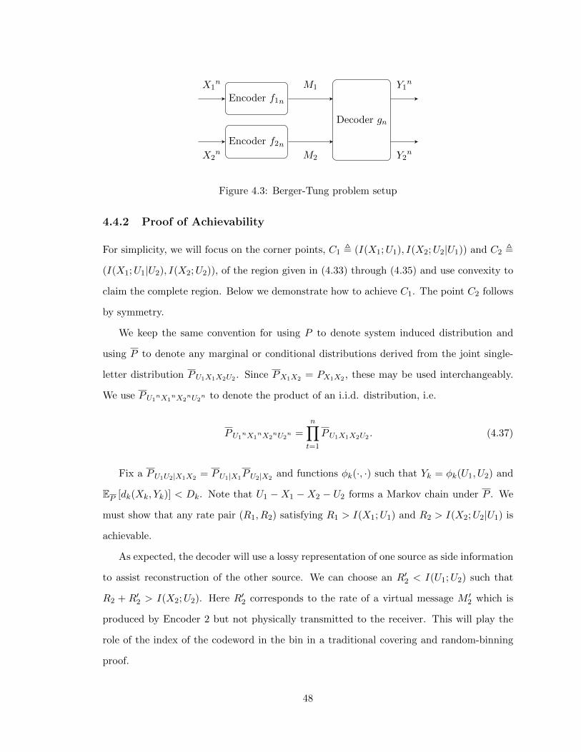
Encoder f1n
Encoder f2n
Decoder gn
X1n
X2n
M1
M2
Y1n
Y2n
Figure 4.3: Berger-Tung problem setup
4.4.2 Proof of Achievability
For simplicity, we will focus on the corner points, C1 , (I(X1;U1), I(X2;U2|U1)) and C2 ,
(I(X1;U1|U2), I(X2;U2)), of the region given in (4.33) through (4.35) and use convexity to
claim the complete region. Below we demonstrate how to achieve C1. The point C2 follows
by symmetry.
We keep the same convention for using P to denote system induced distribution and
using P to denote any marginal or conditional distributions derived from the joint single-
letter distribution PU1X1X2U2 . Since PX1X2 = PX1X2 , these may be used interchangeably.
We use PU1nX1
nX2nU2
n to denote the product of an i.i.d. distribution, i.e.
PU1nX1
nX2nU2
n =
n∏t=1
PU1X1X2U2 . (4.37)
Fix a PU1U2|X1X2= PU1|X1
PU2|X2and functions φk(·, ·) such that Yk = φk(U1, U2) and
EP [dk(Xk, Yk)] < Dk. Note that U1 −X1 −X2 − U2 forms a Markov chain under P . We
must show that any rate pair (R1, R2) satisfying R1 > I(X1;U1) and R2 > I(X2;U2|U1) is
achievable.
As expected, the decoder will use a lossy representation of one source as side information
to assist reconstruction of the other source. We can choose an R′2 < I(U1;U2) such that
R2 + R′2 > I(X2;U2). Here R′2 corresponds to the rate of a virtual message M ′2 which is
produced by Encoder 2 but not physically transmitted to the receiver. This will play the
role of the index of the codeword in the bin in a traditional covering and random-binning
proof.
48
First we will use the likelihood encoder derived from PX1U1 and a random codebook
{u1n(m1)} generated according to PU1 for Encoder 1. Then we will use the likelihood
encoder derived from PX2U2 and another random codebook {u2n(m2,m
′2)} generated ac-
cording to PU2 for Encoder 2. The decoder will use the transmitted message M1 to decode
U1n, as in the point-to-point case, and use the transmitted message M2 along with the
decoded U1n to decode M ′2 as M ′2, as in the Wyner-Ziv case, and reproduce un2 (M2, M
′2).
Finally, the decoder outputs the reconstructions Ykn according to the symbol-by-symbol
functions φk(·, ·) of U1n and U2
n.
The distribution induced by the encoders and decoder is
PX1nX2
nU1nM1M2M ′2M
′2Y1
nY2n = PX1
nX2nP1P2 (4.38)
where
P1(m1, u1n|x1
n)
, PM1|X1n(m1|x1
n)PU1n|M1
(u1n|m1) (4.39)
, PLE1(m1|x1n)PD1(u1
n|m1) (4.40)
and
P2(m2,m′2, m
′2, y1
n, y2n|x2
n, u1n)
, PM2M ′2|X2n(m2,m
′2|x2
n)PM ′2|M2U1n(m′2|m2, u1
n)∏k=1,2
PYkn|U1nM2M ′2
(ykn|u1
n,m2, m′2) (4.41)
, PLE2(m2,m′2|x2
n)PD2(m′2|m2, u1n)∏
k=1,2
PΦ,k(ykn|u1
n,m2, m′2), (4.42)
where PLE1 and PLE2 are the likelihood encoders; PD1 is the first part of the decoder that
does a codeword lookup on C(n)1 ; PD2 is the second part of the decoder that decodes m′2 as
m′2; and PΦ,k(ykn|u1
n,m2, m′2) is the third part of the decoder that reconstructs the source
sequences.
49
We now restate the behavior of the encoders and decoder, as components of the induced
distribution.
Codebook generation: We independently generate 2nR1 sequences in U1n according
to∏nt=1 PU1(u1t) and index them by m1 ∈ [1 : 2nR1 ], and independently generate 2n(R2+R′2)
sequences in U2n according to
∏nt=1 PU2(u2t) and index them by (m2,m
′2) ∈ [1 : 2nR2 ]× [1 :
2nR′2 ]. We use C(n)
1 and C(n)2 to denote the two random codebooks, respectively.
Encoders: The first encoder PLE1(m1|x1n) is the likelihood encoder according to
PX1nU1
n and C(n)1 . The second encoder PLE2(m2,m
′2|x2
n) is the likelihood encoder ac-
cording to PX2nU2
n and C(n)2 .
Decoder: First, let PD1(u1n|m1) be a C(n)
1 codeword lookup decoder. Then, let
PD2(m′2|m2, u1n) be a good channel decoder with respect to the sub-codebook C(n)
2 (m2) =
{u2n(m2, a)}a and the memoryless channel PU1|U2
. Last, define φkn(u1
n, u2n) as the con-
catenation {φk(u1t, u2t)}nt=1 and set the decoders PΦ,k to be the deterministic functions
PΦ,k(ykn|u1
n,m2, m′2) , 1{ykn = φk
n(u1n, U2
n(m2, m′2))}. (4.43)
Analysis: We will need the following distributions: the induced distribution P and
auxiliary distributions Q1 and Q∗1. The general idea of the proof is as follows: Encoder 1
makes P and Q1 close in total variation. Distribution Q∗1 (random only with respect to
the second codebook C(n)2 ) is the expectation of Q1 over the random codebook C(n)
1 . This
is really the key step in the proof. By considering the expectation of the distribution with
respect to C(n)1 , we effectively remove Encoder 1 from the problem and turn the message
from Encoder 1 into memoryless side information at the decoder. Hence, the two distortions
(averaged over C(n)1 ) under P are roughly the same as the distortions under Q∗1, which is a
much simpler distribution. We then recognize Q∗1 as precisely P in (4.10) from the Wyner-
Ziv proof of the previous section, with a source pair (X1, X2), a pair of reconstructions
(Y1, Y2) and U1 as the side information.
1) The auxiliary distribution Q1 takes the following form:
Q1X1nX2
nU1nM1M2M ′2M
′2Y1
nY2n = Q1M1U1
nX1nX2
nP2 (4.44)
50
where
Q1M1U1nX1
nX2n(m1, u1
n, x1n, x2
n)
=1
2nR11{u1
n = U1n(m1)}PX1
n|U1n(x1
n|u1n)PX2
n|X1n(x2
n|x1n). (4.45)
Note that Q1 is the idealized distribution with respect to the first message, as introduced
in the point-to-point case. Hence, by the same arguments, since R1 > I(X1;U1), using the
basic soft-covering lemma (Lemma 2.1),
EC(n)1
[‖Q1 −P‖TV ] ≤ ε1n, (4.46)
where Q1 and P are distributions over random variablesX1n, X2
n, U1n,M1,M2,M
′2, M
′2, Y1
n, Y2n
and ε1n is the error term introduced from the soft-covering lemma.
2) Taking the expectation over codebook C(n)1 , we define
Q∗1X1nX2
nU1nM2M ′2M
′2Y1
nY2n , EC(n)
1
[Q1X1
nX2nU1
nM2M ′2M′2Y1
nY2n
]. (4.47)
Note that under this definition of Q∗1, we have
Q∗1X1nX2
nU1nM2M ′2M
′2Y1
nY2n(x1
n, x2n, u1
n,m2,m′2, m
′2, y1
n, y2n)
= EC(n)1
[Q∗1X1
nX2nU1
n(x1n, x2
n, u1n)]P2(m2,m
′2, m
′2, y1
n, y2n|x2
n, u1n) (4.48)
= PX1nX2
nU1n(x1
n, x2n, u1
n)P2(m2,m′2, m
′2, y1
n, y2n|x2
n, u1n), (4.49)
where the last step can be verified using the same technique as (3.13) given in Section 3.3.
51
By Property 2.1(b),
EC(n)1
[EP [dk(Xkn, Yk
n)]]
≤ EC(n)1
[EQ1 [dk(Xkn, Yk
n)]] + dkmaxε1n (4.50)
= EC(n)1
[ ∑xkn,ykn
Q1XnY n(xkn, yk
n)dk(xkn, yk
n)
]+ dkmaxε1n (4.51)
=∑
xkn,ykn
EC(n)1
[Q1XnY n(xkn, yk
n)]dk(xkn, yk
n) + dkmaxε1n (4.52)
=∑
xkn,ykn
Q∗1XnY n(xkn, yk
n)dk(xkn, yk
n) + dkmaxε1n (4.53)
= EQ∗1[dk(Xk
n, Ykn)] + dkmaxε1n. (4.54)
Note that Q∗1 is exactly of the form of the induced distribution P in the Wyner-Ziv
proof of the previous section, with the inconsequential modification that there are two
reconstructions and two distortion functions. Thus, by (4.19) through (4.30), we obtain
EC(n)2
[EQ∗1
[dk(Xkn, Yk
n)]]
≤ EP [dk(Xk, Yk)] + dkmax(ε2n + δn), (4.55)
where ε2n and δn are error terms introduced from the soft-covering lemma and channel
decoding, respectively.
Finally, taking expectation over C(n)1 and using (4.54) and (4.55),
EC(n)2
[EC(n)
1
[EP [dk(Xkn, Yk
n)]]]
≤ EC(n)2
[EQ∗1
[dk(Xkn, Yk
n)] + dkmaxε1n]
(4.56)
≤ EP [dk(Xk, Yk)] + dkmaxε1n + dkmax(ε2n + δn), (4.57)
where (4.56) follows from (4.54); and (4.57) follows from (4.54) and (4.55). Taking the limit
on both sides gives:
lim supn→∞
EC(n)2
[EC(n)
1
[EP [dk(Xkn, Yk
n)]]]≤ Dk (4.58)
52
�
Remark 3. Note that the proof above uses the proof of Wyner-Ziv achievability from the
previous section. To do the entire proof step by step, we would define a total of three
auxiliary distributions, which would be the Q1 used in the proof, as well as Q(1)2 and Q
(2)2
defined below for completeness. The steps outlined above show how to relate the induced
distribution P to Q1 and its expectation Q∗1. This effectively converts the message from
Encoder 1 into memoryless side information at the decoder. The omitted steps, as seen in
the previous section, relate Q∗1 to Q(1)2 through the soft-covering lemma and Q
(1)2 to Q
(2)2
through reliable channel decoding. The expected value of Q(2)2 over codebooks is the desired
distribution P . For reference, the omitted auxiliary distributions are
Q2M2M ′2U2nX2
nX1nU1
n(m2,m′2, u2
n, x2n, x1
n, u1n)
=1
2n(R2+R′2)1{u2
n = U2n(m2,m
′2)}PX2
n|U2n(x2
n|u2n)
PX1nU1
n|X2n(x1
n, u1n|x2
n), (4.59)
which is of the same structure as the idealized distribution described in Fig. 4.2, and
Q(1)2 X1
nX2nU1
nM2M ′2M′2Y1
nY2n , Q2X1
nX2nU1
nM2M ′2(x1
n, x2n, u1
n,m2,m′2)
PD2(m′2|m2, u1n)∏k=1,2
PΦ,k(ykn|u1
n,m2, m′2) (4.60)
Q(2)2 X1
nX2nU1
nM2M ′2M′2Y1
nY2n , Q2X1
nX2nU1
nM2M ′2(x1
n, x2n, u1
n,m2,m′2)
PD2(m′2|m2, u1n)∏k=1,2
PΦ,k(ykn|u1
n,m2,m′2). (4.61)
Remark 4. To see how this is a simpler proof than the traditional joint typicality encoder
proof, recall from [10] that to bound the different error events, we would need the regular
covering lemma, the conditional typicality lemma, the Markov lemma, and the mutual pack-
ing lemma, some of which are quite involving to verify. With the likelihood encoder, all we
need is the soft-covering lemma and Lemma 4.1.
53

4.5 Summary
In this chapter, we have used the likelihood encoder to obtain achievability results for
multiuser lossy source coding problems. The simplicity of the analysis is accentuated when
used for distributed source coding because it bypasses the need for a Markov lemma of
any form and it avoids the technical complications that can arise in analyzing the decoder
whenever random binning is involved in lossy compression. Although we only demonstrate
with two cases, the Wyner-Ziv and the Berger-Tung settings, it is believed that the likelihood
encoder and its corresponding analysis can achieve other best known source coding results.
A highlight in the achievability proof for the Wyner-Ziv setting is that we are able to apply
the channel coding result directly without the need for a packing lemma. This becomes an
important feature in proving secrecy results in the next chapters.
54

Chapter 5
Rate-Distortion Based Security in
the Noiseless Wiretap Channel
5.1 Introduction
In this chapter, we investigate secrecy in source coding problems from a rate-distortion
approach. We first review Shannon’s formulation of perfect secrecy in lossy compression
using a shared secret key, where the secrecy performance is measured by a quantity called
“equivocation”. Then we introduce Yamamoto’s rate-distortion based formulation of the
same communication system. We refer to this model as the naive formulation, because it
does not ensure a strong secure communication system. However, this naive formulation
remains an important game-theoretic setting. In particular, the model captures the essence
of a system where the legitimate receiver and eavesdropper are each only given one attempt
to estimate the source. Next, we apply this naive secrecy formulation to physical layer
security where instead of a shared secret key, the legitimate receiver and the eavesdropper
have access to side information that is correlated with the source.
At the end of the chapter, we strengthen the formulation by causally disclosing the
source realization to the eavesdropper during decoding. It turns out this modification
not only provides a stable secure communication system, but also fully generalizes the
equivocation formulation. Although these two metrics, equivocation and distortion, appear
55
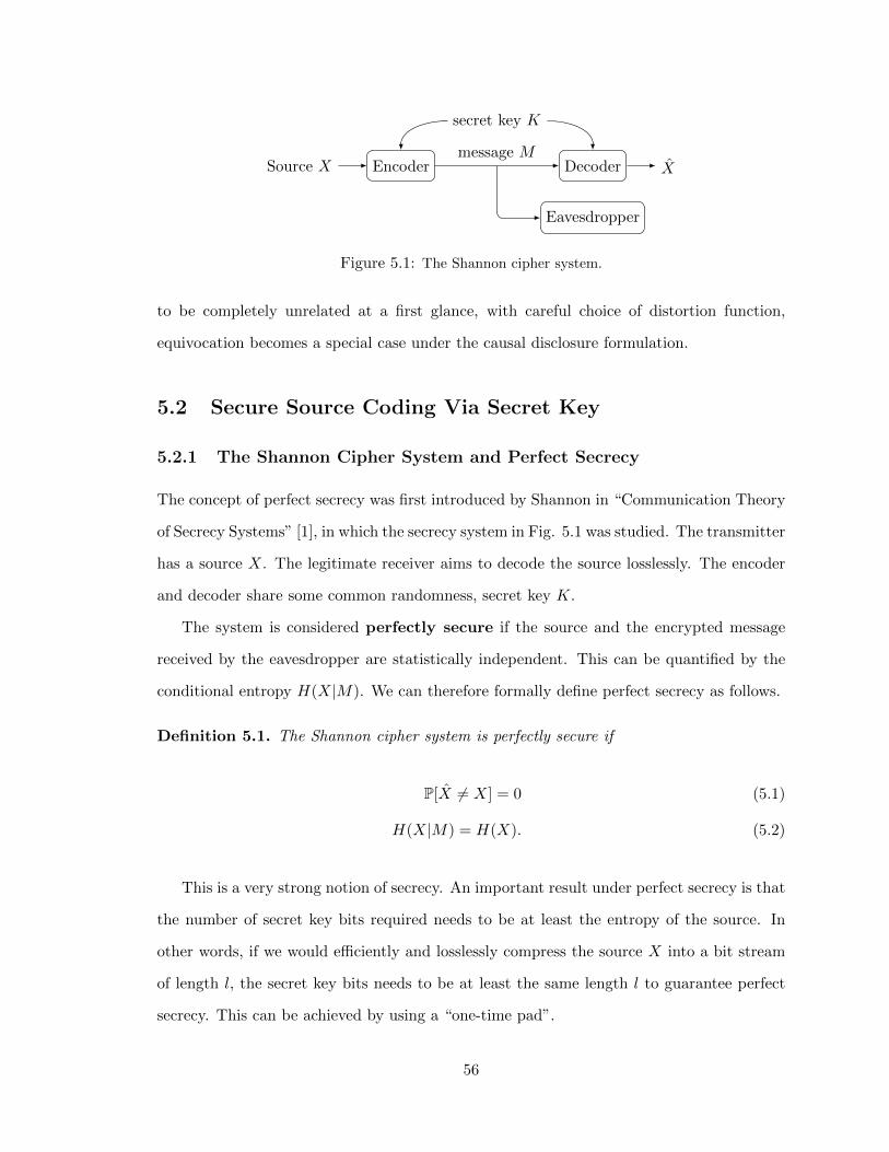
Source X Encoder Decoder X
secret key K
Eavesdropper
message M
Figure 5.1: The Shannon cipher system.
to be completely unrelated at a first glance, with careful choice of distortion function,
equivocation becomes a special case under the causal disclosure formulation.
5.2 Secure Source Coding Via Secret Key
5.2.1 The Shannon Cipher System and Perfect Secrecy
The concept of perfect secrecy was first introduced by Shannon in “Communication Theory
of Secrecy Systems” [1], in which the secrecy system in Fig. 5.1 was studied. The transmitter
has a source X. The legitimate receiver aims to decode the source losslessly. The encoder
and decoder share some common randomness, secret key K.
The system is considered perfectly secure if the source and the encrypted message
received by the eavesdropper are statistically independent. This can be quantified by the
conditional entropy H(X|M). We can therefore formally define perfect secrecy as follows.
Definition 5.1. The Shannon cipher system is perfectly secure if
P[X 6= X] = 0 (5.1)
H(X|M) = H(X). (5.2)
This is a very strong notion of secrecy. An important result under perfect secrecy is that
the number of secret key bits required needs to be at least the entropy of the source. In
other words, if we would efficiently and losslessly compress the source X into a bit stream
of length l, the secret key bits needs to be at least the same length l to guarantee perfect
secrecy. This can be achieved by using a “one-time pad”.
56
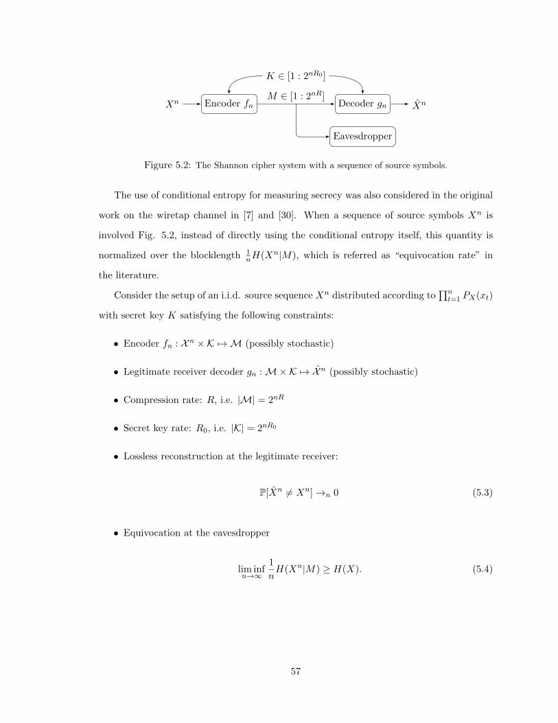
Xn Encoder fn Decoder gn Xn
K ∈ [1 : 2nR0 ]
Eavesdropper
M ∈ [1 : 2nR]
Figure 5.2: The Shannon cipher system with a sequence of source symbols.
The use of conditional entropy for measuring secrecy was also considered in the original
work on the wiretap channel in [7] and [30]. When a sequence of source symbols Xn is
involved Fig. 5.2, instead of directly using the conditional entropy itself, this quantity is
normalized over the blocklength 1nH(Xn|M), which is referred as “equivocation rate” in
the literature.
Consider the setup of an i.i.d. source sequence Xn distributed according to∏nt=1 PX(xt)
with secret key K satisfying the following constraints:
• Encoder fn : X n ×K 7→M (possibly stochastic)
• Legitimate receiver decoder gn :M×K 7→ X n (possibly stochastic)
• Compression rate: R, i.e. |M| = 2nR
• Secret key rate: R0, i.e. |K| = 2nR0
• Lossless reconstruction at the legitimate receiver:
P[Xn 6= Xn]→n 0 (5.3)
• Equivocation at the eavesdropper
lim infn→∞
1
nH(Xn|M) ≥ H(X). (5.4)
57
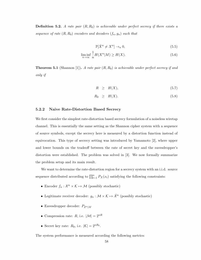
Definition 5.2. A rate pair (R,R0) is achievable under perfect secrecy if there exists a
sequence of rate (R,R0) encoders and decoders (fn, gn) such that
P[Xn 6= Xn]→n 0, (5.5)
lim infn→∞
1
nH(Xn|M) ≥ H(X). (5.6)
Theorem 5.1 (Shannon [1]). A rate pair (R,R0) is achievable under perfect secrecy if and
only if
R ≥ H(X), (5.7)
R0 ≥ H(X). (5.8)
5.2.2 Naive Rate-Distortion Based Secrecy
We first consider the simplest rate-distortion based secrecy formulation of a noiseless wiretap
channel. This is essentially the same setting as the Shannon cipher system with a sequence
of source symbols, except the secrecy here is measured by a distortion function instead of
equivocation. This type of secrecy setting was introduced by Yamamoto [2], where upper
and lower bounds on the tradeoff between the rate of secret key and the eavesdropper’s
distortion were established. The problem was solved in [3]. We now formally summarize
the problem setup and its main result.
We want to determine the rate-distortion region for a secrecy system with an i.i.d. source
sequence distributed according to∏nt=1 PX(xt) satisfying the following constraints:
• Encoder fn : X n ×K 7→M (possibly stochastic)
• Legitimate receiver decoder: gn :M×K 7→ X n (possibly stochastic)
• Eavesdropper decoder: PZn|M
• Compression rate: R, i.e. |M| = 2nR
• Secret key rate: R0, i.e. |K| = 2nR0 .
The system performance is measured according the following metrics:
58
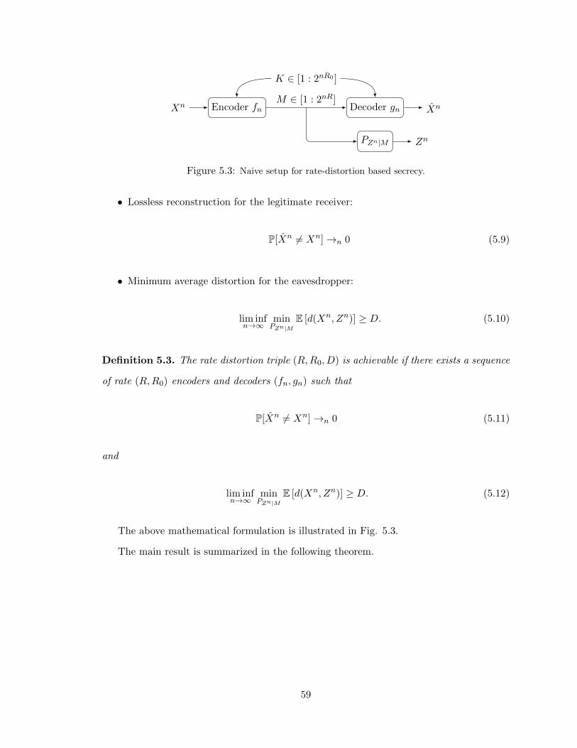
Xn Encoder fn Decoder gn Xn
K ∈ [1 : 2nR0 ]
PZn|M Zn
M ∈ [1 : 2nR]
Figure 5.3: Naive setup for rate-distortion based secrecy.
• Lossless reconstruction for the legitimate receiver:
P[Xn 6= Xn]→n 0 (5.9)
• Minimum average distortion for the eavesdropper:
lim infn→∞
minPZn|M
E [d(Xn, Zn)] ≥ D. (5.10)
Definition 5.3. The rate distortion triple (R,R0, D) is achievable if there exists a sequence
of rate (R,R0) encoders and decoders (fn, gn) such that
P[Xn 6= Xn]→n 0 (5.11)
and
lim infn→∞
minPZn|M
E [d(Xn, Zn)] ≥ D. (5.12)
The above mathematical formulation is illustrated in Fig. 5.3.
The main result is summarized in the following theorem.
59
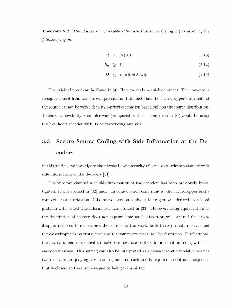
Theorem 5.2. The closure of achievable rate-distortion triple (R,R0, D) is given by the
following region:
R ≥ H(X), (5.13)
R0 ≥ 0, (5.14)
D ≤ minz
E[d(X, z)]. (5.15)
The original proof can be found in [3]. Here we make a quick comment. The converse is
straightforward from lossless compression and the fact that the eavesdropper’s estimate of
the source cannot be worse than its a-priori estimation based only on the source distribution.
To show achievability, a simpler way (compared to the scheme given in [3]) would be using
the likelihood encoder with its corresponding analysis.
5.3 Secure Source Coding with Side Information at the De-
coders
In this section, we investigate the physical layer security of a noiseless wiretap channel with
side information at the decoders [31].
The wire-tap channel with side information at the decoders has been previously inves-
tigated. It was studied in [32] under an equivocation constraint at the eavesdropper and a
complete characterization of the rate-distortion-equivocation region was derived. A related
problem with coded side information was studied in [33]. However, using equivocation as
the description of secrecy does not capture how much distortion will occur if the eaves-
dropper is forced to reconstruct the source. In this work, both the legitimate receiver and
the eavesdropper’s reconstructions of the source are measured by distortion. Furthermore,
the eavesdropper is assumed to make the best use of its side information along with the
encoded message. This setting can also be interpreted as a game-theoretic model where the
two receivers are playing a zero-sum game and each one is required to output a sequence
that is closest to the source sequence being transmitted.
60
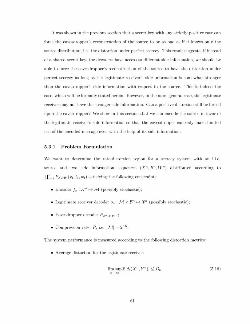
It was shown in the previous section that a secret key with any strictly positive rate can
force the eavesdropper’s reconstruction of the source to be as bad as if it knows only the
source distribution, i.e. the distortion under perfect secrecy. This result suggests, if instead
of a shared secret key, the decoders have access to different side information, we should be
able to force the eavesdropper’s reconstruction of the source to have the distortion under
perfect secrecy as long as the legitimate receiver’s side information is somewhat stronger
than the eavesdropper’s side information with respect to the source. This is indeed the
case, which will be formally stated herein. However, in the more general case, the legitimate
receiver may not have the stronger side information. Can a positive distortion still be forced
upon the eavesdropper? We show in this section that we can encode the source in favor of
the legitimate receiver’s side information so that the eavesdropper can only make limited
use of the encoded message even with the help of its side information.
5.3.1 Problem Formulation
We want to determine the rate-distortion region for a secrecy system with an i.i.d.
source and two side information sequences (Xn, Bn,Wn) distributed according to∏nt=1 PXBW (xt, bt, wt) satisfying the following constraints:
• Encoder fn : X n 7→ M (possibly stochastic);
• Legitimate receiver decoder gn :M×Bn 7→ Yn (possibly stochastic);
• Eavesdropper decoder PZn|MWn ;
• Compression rate: R, i.e. |M| = 2nR.
The system performance is measured according to the following distortion metrics:
• Average distortion for the legitimate receiver:
lim supn→∞
E[db(Xn, Y n)] ≤ Db (5.16)
61
Encoder fn Decoder gn
PZn|MWn
Xn M Y n
Bn
Zn
Wn
Figure 5.4: Secrecy system setup with side information at the decoders.
• Minimum average distortion for the eavesdropper:
lim infn→∞
minPZn|MWn
E[dw(Xn, Zn)] ≥ Dw (5.17)
Note that db and dw can be the same or different distortion measures.
Definition 5.4. The rate-distortion triple (R,Db, Dw) is achievable if there exists a se-
quence of rate R encoders and decoders (fn, gn) such that
lim supn→∞
E[db(Xn, Y n)] ≤ Db (5.18)
and
lim infn→∞
minPZn|MWn
E[dw(Xn, Zn)] ≥ Dw. (5.19)
The above mathematical formulation is illustrated in Fig. 5.4.
For the special case of lossless compression between the transmitter and the legitimate
receiver, we make the following definition.
Definition 5.5. A rate-distortion pair (R,Dw) is achievable if there exists a sequence of
encoders and decoders (fn, gn) such that
P [Xn 6= Y n]→n 0 (5.20)
62
and
lim infn→∞
minPZn|M,Wn
E[dw(Xn, Zn)] ≥ Dw. (5.21)
Less Noisy and More Capable Side Information
Definition 5.6. The side information B is strictly less noisy than the side information
W with respect to X if
I(V ;B) > I(V ;W )
for all V such that V −X − (B,W ) and I(V ;B) > 0.
Definition 5.7. The side information B is strictly more capable than the side information
W with respect to X if
I(X;B) > I(X;W ).
5.3.2 Inner Bound
Theorem 5.3. A rate-distortion triple (R,Db, Dw) is achievable if
R > I(V ;X|B) (5.22)
Db ≥ E[db(X,Y )] (5.23)
Dw ≤ minz(u,w)
E[dw(X,Z(U,W ))] (5.24)
I(V ;B|U) > I(V ;W |U) (5.25)
for some PUV XBW = PXBWPV |XPU |V , where Y = φ(V,B) for some function φ(·, ·).
Theorem 5.3 involves two auxiliary variables U and V that are correlated with the
source X in a Markov chain relationship. The variable V can be understood as the lossy
representation of X that is communicated efficiently using random binning to the intended
receiver, which will be used with the side information B to estimate X, just as in the setting
without an eavesdropper which was pioneered by [27]. The purpose of the auxiliary variable
U is to provide secrecy similar to the way secrecy is achieved in [32]. The side information
at the intended receiver must be better than that of the eavesdropper (as measured by
63
mutual information with V ) in order to prevent decoding of V . The variable U (if needed)
is given away to all parties as the first layer of a superposition code in order to generate
this condition for V .
We now give the achievability proof of Theorem 5.3 using the soft-covering lemmas. We
apply the same proof technique using the likelihood encoder as introduced in Chapter 3
with the modification of using a superposition codebook.
The source is encoded into four messages Mp, M′p, Ms and M ′s, where Mp and Ms
are transmitted and M ′p and M ′s are virtual messages that are not physically transmitted,
but will be recovered with small error at the legitimate receiver with the help of the side
information. On the other hand, Mp and M ′p play the role of public messages, which both
the legitimate receiver and the eavesdropper will decode; Ms and M ′s index a codeword that
is kept secret from the eavesdropper, which only the legitimate receiver can make sense of
with its own side information.
The P notation is used in the same way as in the previous chapters and P is used to
denote the system induced distribution. Note that PXBW = PXBW .
Proof. Fix a distribution PUV XBW = PXBWP V |XPU |V satisfying
I(V ;B|U) > I(V ;W |U), (5.26)
EP [db(X,φ(V,B))] ≤ Db, (5.27)
minz(u,w)
EP [dw(X,Z(U,W ))] ≥ Dw, (5.28)
and fix rates Rp, R′p, Rs, R
′s such that
Rp +R′p > I(U ;X), (5.29)
R′p < I(U ;B), (5.30)
Rs +R′s > I(X;V |U), (5.31)
I(V ;W |U) < R′s < I(V ;B|U). (5.32)
64
The distribution induced by the encoder and decoder is
P(xn, bn, wn,mp,m′p,ms,m
′s, m
′p, m
′s, y
n)
, PXnBnWn(xn, bn, wn)PLE(mp,m′p,ms,m
′s|xn)
PD(m′p, m′s|mp,ms, b
n)PΦ(yn|mp, m′p,ms, m
′s, b
n), (5.33)
where PLE(mp,m′p,ms,m
′s|xn) is the source encoder; PD(m′p, m
′s|mp,ms, b
n) is the first
part of the decoder that estimates m′p and m′s as m′p and m′s; PΦ(yn|mp, m′p,ms, m
′s, b
n) is
the second part of the decoder that reconstructs the source sequence.
Codebook generation: We independently generate 2n(Rp+R′p) sequences in Un ac-
cording to∏nt=1 PU (ut) and index by (mp,m
′p) ∈ [1 : 2nRp ] × [1 : 2nR
′p ]. We use C(n)
U to
denote this random codebook. For each (mp,m′p) ∈ [1 : 2nRp ]× [1 : 2nR
′p ], we independently
generate 2n(Rs+R′s) sequences in Vn according to∏nt=1 P V |U (vt|ut(mp,m
′p)) and index by
(mp,m′p,ms,m
′s), (ms,m
′s) ∈ [1 : 2nRs ] × [1 : 2nR
′s ]. We use C(n)
V (mp,m′p) to denote this
random codebook.
Encoder: The encoder PLE(mp,m′p,ms,m
′s|xn) is a likelihood encoder that chooses
Mp,M′p,Ms,M
′s stochastically according to the following probability:
PLE(m|xn) =L(m|xn)∑
m∈M L(m|xn)(5.34)
where m = (mp,m′p,ms,m
′s), M = [1 : 2nRp ]× [1 : 2nR
′p ]× [1 : 2nRs ]× [1 : 2nR
′s ], and
L(m|xn) = PXn|V n(xn|vn(m)). (5.35)
Decoder: The decoder has two parts. Let PD(m′p, m′s|mp,ms, b
n) be a good channel
decoder with respect to the superposition sub-codebook {vn(mp, ap,ms, as)}ap,as and the
memoryless channel PB|V . For the second part of the decoder, fix a function φ(·, ·). Define
φn(vn, bn) as the concatenation {φ(vt, bt)}nt=1 and set the decoder PΦ to be the deterministic
65
function
PΦ(yn|mp, m′p,ms, m
′s, b
n)
, 1{yn = φn(vn(mp, m′p,ms, m
′s), b
n)}. (5.36)
Analysis: We examine the distortions at the two receivers one at a time. To analyze
the distortion at the legitimate receiver, we will consider four distributions, the induced
distribution P, two approximating distributions Q(1) and Q(2), and an auxiliary distribution
Q′ that helps with the analysis. The idea is to show that 1) the system has nice behavior
for distortion under Q(2); and 2) P and Q(2) are close in total variation (on average over
the random codebook) through Q(1). To analyze the distortion at the eavesdropper, we will
consider the induced distribution P together with an auxiliary distribution Q.
Distortion at the Legitimate Receiver
This part of the proof follows the same idea of the achievability proof for the Wyner-Ziv
setting using the likelihood encoder given in Section 4.3.2.
The approximating distributions Q(1) and Q(2) are defined through an idealized distri-
bution Q of the structure given in Fig. 5.5. This idealized distribution Q can be written
as
QXnBnWnMpM ′pMsM ′sUnV n(xn, bn, wn,mp,m
′p,ms,m
′s, u
n, vn)
= QMpM ′pMsM ′s(mp,m′p,ms,m
′s)QUn|MpM ′p
(un|mp,m′p)QV n|UnMsM ′s
(vn|un,ms,m′s)
QXnBnWn|MpM ′pMsM ′s(xn, bn, wn|mp,m
′p,ms,m
′s) (5.37)
=1
2n(Rp+R′p+Rs+R′s)1{un = Un(mp,m
′p)}1{vn = V n(mp,m
′p,ms,m
′s)}
PXnBnWn|V n(xn, bn, wn|V n(mp,m′p,ms,m
′s)) (5.38)
=1
2n(Rp+R′p+Rs+R′s)1{un = Un(mp,m
′p)}1{vn = V n(mp,m
′p,ms,m
′s)}
n∏t=1
PX|V (xt|vt)PBW |X(bt, wt|xt), (5.39)
where (5.39) follows from the Markov relation V −X −BW .
66
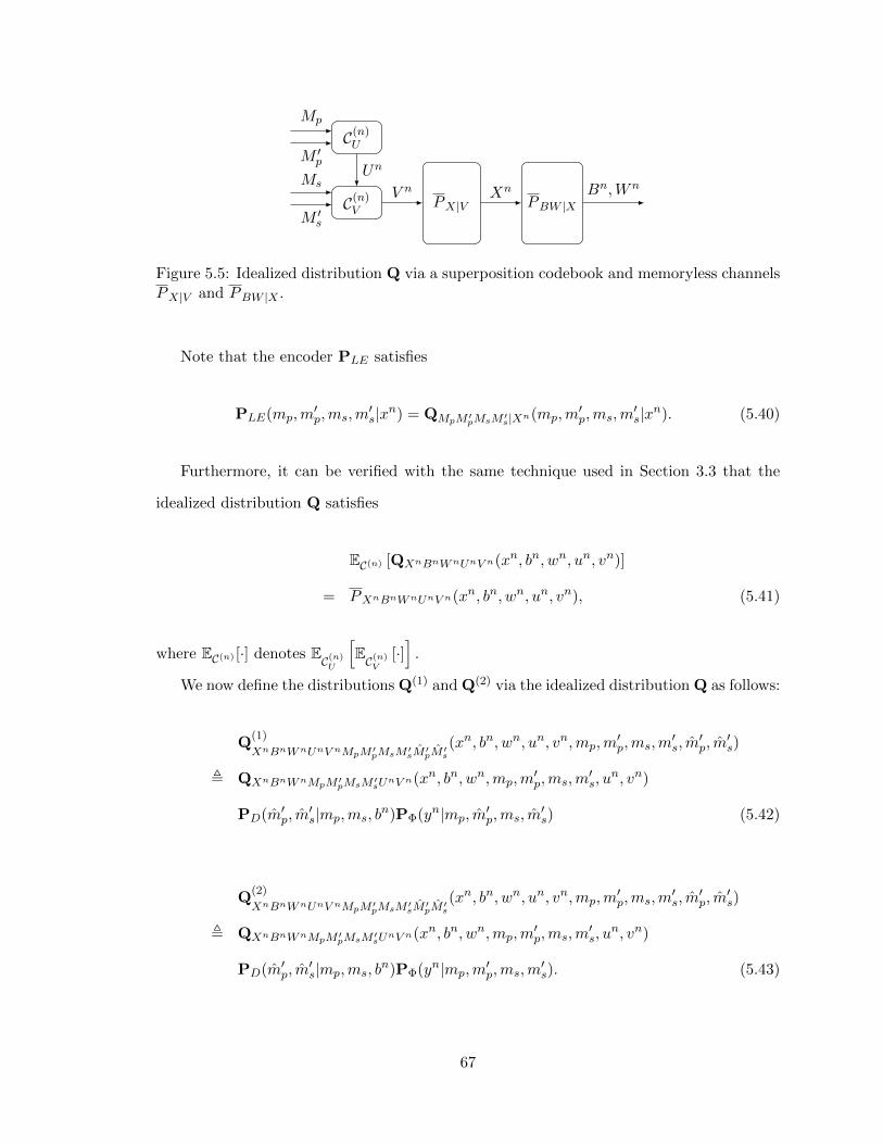
C(n)U
C(n)V
PX|V PBW |X
Mp
M ′pMs
M ′s
Un
V n Xn Bn,Wn
Figure 5.5: Idealized distribution Q via a superposition codebook and memoryless channelsPX|V and PBW |X .
Note that the encoder PLE satisfies
PLE(mp,m′p,ms,m
′s|xn) = QMpM ′pMsM ′s|Xn(mp,m
′p,ms,m
′s|xn). (5.40)
Furthermore, it can be verified with the same technique used in Section 3.3 that the
idealized distribution Q satisfies
EC(n) [QXnBnWnUnV n(xn, bn, wn, un, vn)]
= PXnBnWnUnV n(xn, bn, wn, un, vn), (5.41)
where EC(n) [·] denotes EC(n)U
[EC(n)
V
[·]].
We now define the distributions Q(1) and Q(2) via the idealized distribution Q as follows:
Q(1)
XnBnWnUnV nMpM ′pMsM ′sM′pM′s
(xn, bn, wn, un, vn,mp,m′p,ms,m
′s, m
′p, m
′s)
, QXnBnWnMpM ′pMsM ′sUnV n(xn, bn, wn,mp,m
′p,ms,m
′s, u
n, vn)
PD(m′p, m′s|mp,ms, b
n)PΦ(yn|mp, m′p,ms, m
′s) (5.42)
Q(2)
XnBnWnUnV nMpM ′pMsM ′sM′pM′s
(xn, bn, wn, un, vn,mp,m′p,ms,m
′s, m
′p, m
′s)
, QXnBnWnMpM ′pMsM ′sUnV n(xn, bn, wn,mp,m
′p,ms,m
′s, u
n, vn)
PD(m′p, m′s|mp,ms, b
n)PΦ(yn|mp,m′p,ms,m
′s). (5.43)
67
Notice that the distributions Q(1) and Q(2) differ only in PΦ. From (5.41), it can be shown
that the distortion under distribution Q(2) averaged over the random codebook is given by
the following:
EC(n)
[EQ(2) [db(X
n, Y n)]]
=∑
xn,vn,bn
EC(n) [QXnV nBn(xn, vn, bn)] db(xn, φn(vn, bn)) (5.44)
=∑
xn,vn,bn
PXnV nBn(xn, vn, bn)db(xn, φn(vn, bn)) (5.45)
= EP [db(X,Y )] . (5.46)
Define the auxiliary distribution Q′ on a subset of the variables as
Q′MpM ′pXn(mp,m
′p, x
n) ,1
2n(Rp+R′p)PXn|Un(xn|Un(mp,m
′p)). (5.47)
Since Rs+R′s > I(X;V |U), applying the generalized superposition soft-covering lemma
2.2, we have
EC(n)
[∥∥∥QMpM ′pXn −Q′MpM ′pX
n
∥∥∥TV
]≤ e−γ2n , ε2n. (5.48)
Also since Rp +R′p > I(U ;X), applying the basic soft-covering lemma (Lemma 2.1), we
have
EC(n)
[∥∥PXn −Q′Xn
∥∥TV
]≤ e−γ1n , ε1n. (5.49)
Using Property 2.1(b), (5.49), and (5.48), we obtain
EC(n) [‖QXn − PXn‖TV ] ≤ ε1n + ε2n , ε3n. (5.50)
Therefore, by definitions of P and Q(1) and Property 2.1(c), we have
EC(n)
[∥∥∥P−Q(1)∥∥∥TV
]≤ ε3n (5.51)
68
where the distributions are taken over XnBnWnMpM′pMsM
′sM′pM′sY
n.
On the one hand, we need to apply the Wyner-Ziv technique to complete the distortion
bound at the legitimate receiver. Since R′p < I(U ;B) and R′s < I(V ;B|U), the codebooks
are randomly generated, and M ′p and M ′s are uniformly distributed under Q, it is well
known that the maximum likelihood decoder (as well as a variety of other decoders) will
drive the error probability to zero as n goes to infinity. This can be seen from Fig. 5.5, by
identifying for fixed Mp and Ms, that M ′p and M ′s are the messages to be transmitted over
the memoryless channel PB|V with the superposition codebook. Specifically,
EC(n)
[PQ(1)
[(M ′p, M
′s) 6= (M ′p,M
′s)]]≤ δn →n 0. (5.52)
Using Lemma 4.1, it can be shown that
EC(n)
[∥∥∥∥Q(1)
XnBnWnMpM ′pMsM ′s−Q
(2)XnBnWnMpM ′pMsM ′s
∥∥∥∥TV
]≤ EC(n)
[PQ(1)
[(M ′p, M
′s) 6= (M ′p,M
′s)]]
(5.53)
≤ δn. (5.54)
Hence, by (5.46), (5.51) and (5.54) and Property 2.1(a) and (b), we obtain
EC(n) [EP[db(Xn, Y n)]]
≤ EP [db(X,Y )] + dbmax(ε3n + δn) (5.55)
≤ Db + dbmax(ε3n + δn). (5.56)
This completes the distortion analysis at the legitimate receiver.
Distortion at the Eavesdropper
To evaluate the enforced distortion at the eavesdropper with the best possible decoder,
we will consider two distributions: the system induced distribution P and an auxiliary
69
distribution Q(i) defined as
Q(i)MpM ′pMsM ′sU
nXWn(mp,m′p,ms,m
′s, u
n, x, wn)
,1
2n(Rp+R′p+Rs+R′s)1{un = Un(mp,m
′p)}
n∏t=1
PW |U (wt|Ut(mp,m′p))PX|WU (x|wi, Ui(mp,m
′p)). (5.57)
Note that under Q(i), we have the Markov relation
X − Ui(Mp,M′p)Wi −MpM
′pMsM
′sW
n. (5.58)
The auxiliary distribution Q(i) has the following property:
EC(n)U
[Q
(i)UnWnX(un, wn, x)
]=
n∏t=1
PU (ut)PW |U (wt|ut)PX|WU (x|wi, ui). (5.59)
Recall that under distribution Q, for fixed Ms = ms,
QMpM ′pM′sW
nXi|Ms(mp,m
′p,m
′s, w
n, xi|ms)
=1
2n(Rp+R′p+R′s)PWn|V n(wn|V n(mp,m
′p,ms,m
′s))
PX|WV U (xi|wi, Vi(mp,m′p,ms,m
′s), Ui(mp,m
′p)) (5.60)
Since R′s > I(V ;W |U), by applying the superposition soft-covering lemma 2.2, we have
for fixed ms,
EC(n)
[∥∥∥Q(i)MpM ′pW
nX −QMpM ′pWnXi
∥∥∥TV
]≤ e−γ4n , ε4n. (5.61)
Averaging over Ms, we have
EC(n)
[∥∥∥Q(i)MpM ′pMsWnX −QMpM ′pMsWnXi
∥∥∥TV
]≤ ε4n, (5.62)
70

and by Property 2.1(b), (5.51) and (5.62),
EC(n)
[∥∥∥Q(i)MpM ′pMsWnX −PMpM ′pMsWnXi
∥∥∥TV
]≤ ε3n + ε4n , ε5n. (5.63)
Also note that, since Rp +R′p > 0, we can invoke Lemma 2.2 by identifying
(R1, R2, U, V,X,Z)← (0, Rp +R′p,∅, U,∅, U), (5.64)
where the left side symbols represents the symbols from Lemma 2.2. This gives us
EC(n)
[∥∥∥Q(i)ui(Mp,M ′p) − PU
∥∥∥TV
]≤ e−γ6n , ε6n. (5.65)
Combining (5.56), (5.63) and (5.65), we get
EC(n)
[ n∑i=1
∥∥∥PMpM ′pMsWnXi − Q(i)MpM ′pMsWnX
∥∥∥TV
+
n∑i=1
∥∥∥Q(i)ui(Mp,M ′p) − PU
∥∥∥TV
+ |EP[db(Xn, Y n)]−Db|
]≤ nε5n + nε6n + dbmax(ε3n + δn) (5.66)
≤ ne−nmin(γ1,γ2,γ4,γ6) + dbmax(ε3n + δn) (5.67)
, εn →n 0. (5.68)
Therefore, there exists a codebook under which
n∑i=1
∥∥∥PMpM ′pMsWnXi − Q(i)MpM ′pMsWnX
∥∥∥TV≤ εn, (5.69)
n∑i=1
∥∥∥Q(i)ui(Mp,M ′p) − PU
∥∥∥TV≤ εn, (5.70)
and
EP [db(Xn, Y n)] ≤ Db + εn. (5.71)
71

Finally, the distortion at the eavesdropper can be lower bounded by
minzn(mp,ms,wn)
EP [dw(Xn, zn(Mp,Ms,Wn))]
≥ minzn(mp,m′p,ms,w
n)EP[dw(Xn, zn(Mp,M
′p,Ms,W
n))]
(5.72)
=1
n
n∑i=1
minzi(mp,m′p,ms,w
n)EP[dw(Xi, zi(Mp,M
′p,Ms,W
n))]
(5.73)
≥ 1
n
n∑i=1
minzi(mp,m′p,ms,w
n)EQ(i)
[dw(X, zi(Mp,M
′p,Ms,W
n))]− εndwmax (5.74)
=1
n
n∑i=1
minz(u,w)
EQ(i)
[dw(X, z(ui(Mp,M
′p),Wi))
]− εndwmax (5.75)
≥ 1
n
n∑i=1
minz(u,w)
EP [dw(X, z(U,W ))]− 2εndwmax (5.76)
where (5.75) uses the Markov relation under Q(i) given in (5.58), and (5.76) uses∥∥∥Q(i)ui(Mp,M ′p) − PU
∥∥∥TV≤ εn from (5.70) and the fact that
Q(i)WiX|Ui(wi, x|ui) = PW |U (wi|ui)PX|WU (x|wi, ui) (5.77)
from (5.57).
This completes the distortion analysis at the eavesdropper.
5.3.3 Outer Bound
A tight outer bound is not attained and hence, the optimality of Theorem 5.3 is not yet
known. A trivial outer bound is stated as follows for completeness.
Theorem 5.4. If a rate-distortion triple (R,Db, Dw) is achievable, then
R ≥ I(V ;X|B) (5.78)
Db ≥ E[db(X,Y )] (5.79)
Dw ≤ minz(w)
E[dw(X, z(W ))] (5.80)
for some PV XBW = PXBWPV |X , where Y = φ(V,B) for some function φ(·, ·).
72
Proof. To get (5.78) and (5.79), we just need to apply the Wyner-Ziv converse; and to
get (5.80), observe that the reconstruction cannot be worse than the symbol-by-symbol
estimation of Xn from Wn without using M .
5.3.4 Special Cases
Less Noisy Side Information
Corollary 5.1. If the legitimate receiver has strictly less noisy side information than the
eavesdropper, the converse of Theorem 5.4 is tight.
Proof. To see the achievability, we just need to set the U in Theorem 5.3 to be ∅.
Note that the strictly less noisy condition meets the inequality in Theorem 5.3. Corollary
5.1 covers the case of degraded side information at the eavesdropper, i.e. X−B−W , except
for the corner case where I(X;W ) = I(X;B).
Lossless Compression
When the legitimate receiver must reconstruct the source sequence losslessly, we have the
following inner bound.
Corollary 5.2. (R,Dw) is achievable if
R > H(X|B) (5.81)
Dw ≤ minz(u,w)
E[dw(X, z(U,W ))] (5.82)
I(X;B|U) > I(X;W |U) (5.83)
for some PUXBW = PXBWPU |X .
Proof. This is consistent with Theorem 5.3 by setting V = X and that the additional proof
required for lossless recovery follows naturally from the construction of the achievability
scheme for Theorem 5.3.
Corollary 5.3. If the legitimate receiver has strictly more capable side information than the
eavesdropper with respect to the source, then the rate-distortion pair (R,Dw) is achievable
73
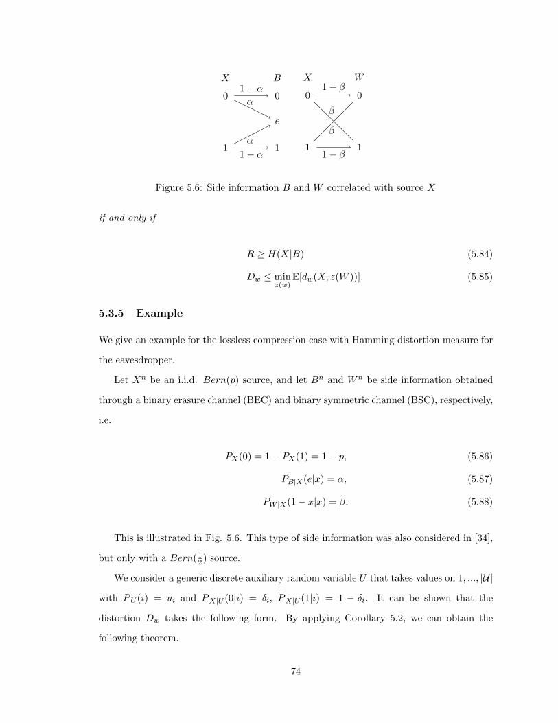
1
0
1
0
e
X B
1− αα
α
1− α
1
0
1
0
X W
1− β
β
β
1− β
Figure 5.6: Side information B and W correlated with source X
if and only if
R ≥ H(X|B) (5.84)
Dw ≤ minz(w)
E[dw(X, z(W ))]. (5.85)
5.3.5 Example
We give an example for the lossless compression case with Hamming distortion measure for
the eavesdropper.
Let Xn be an i.i.d. Bern(p) source, and let Bn and Wn be side information obtained
through a binary erasure channel (BEC) and binary symmetric channel (BSC), respectively,
i.e.
PX(0) = 1− PX(1) = 1− p, (5.86)
PB|X(e|x) = α, (5.87)
PW |X(1− x|x) = β. (5.88)
This is illustrated in Fig. 5.6. This type of side information was also considered in [34],
but only with a Bern(12) source.
We consider a generic discrete auxiliary random variable U that takes values on 1, ..., |U|
with PU (i) = ui and PX|U (0|i) = δi, PX|U (1|i) = 1 − δi. It can be shown that the
distortion Dw takes the following form. By applying Corollary 5.2, we can obtain the
following theorem.
74
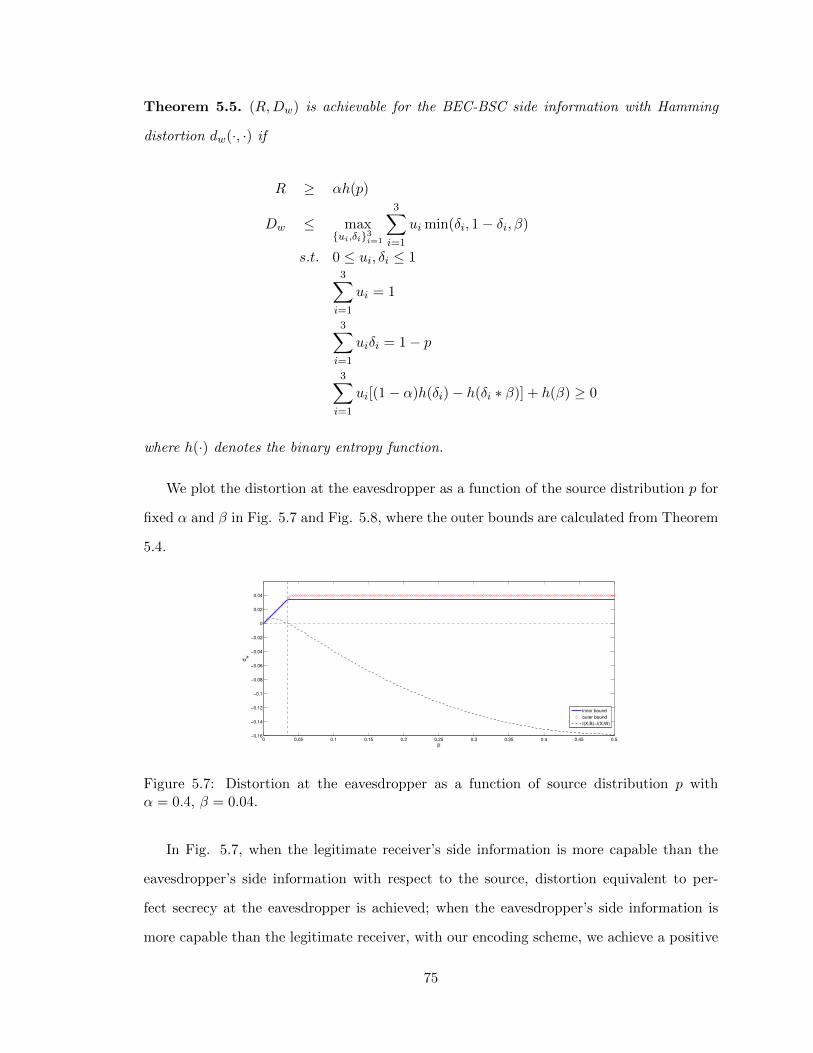
Theorem 5.5. (R,Dw) is achievable for the BEC-BSC side information with Hamming
distortion dw(·, ·) if
R ≥ αh(p)
Dw ≤ max{ui,δi}3i=1
3∑i=1
ui min(δi, 1− δi, β)
s.t. 0 ≤ ui, δi ≤ 13∑i=1
ui = 1
3∑i=1
uiδi = 1− p
3∑i=1
ui[(1− α)h(δi)− h(δi ∗ β)] + h(β) ≥ 0
where h(·) denotes the binary entropy function.
We plot the distortion at the eavesdropper as a function of the source distribution p for
fixed α and β in Fig. 5.7 and Fig. 5.8, where the outer bounds are calculated from Theorem
5.4.
0 0.05 0.1 0.15 0.2 0.25 0.3 0.35 0.4 0.45 0.5−0.16
−0.14
−0.12
−0.1
−0.08
−0.06
−0.04
−0.02
0
0.02
0.04
p
dw
inner bound
outer bound
I(X;B)−I(X;W)
Figure 5.7: Distortion at the eavesdropper as a function of source distribution p withα = 0.4, β = 0.04.
In Fig. 5.7, when the legitimate receiver’s side information is more capable than the
eavesdropper’s side information with respect to the source, distortion equivalent to per-
fect secrecy at the eavesdropper is achieved; when the eavesdropper’s side information is
more capable than the legitimate receiver, with our encoding scheme, we achieve a positive
75
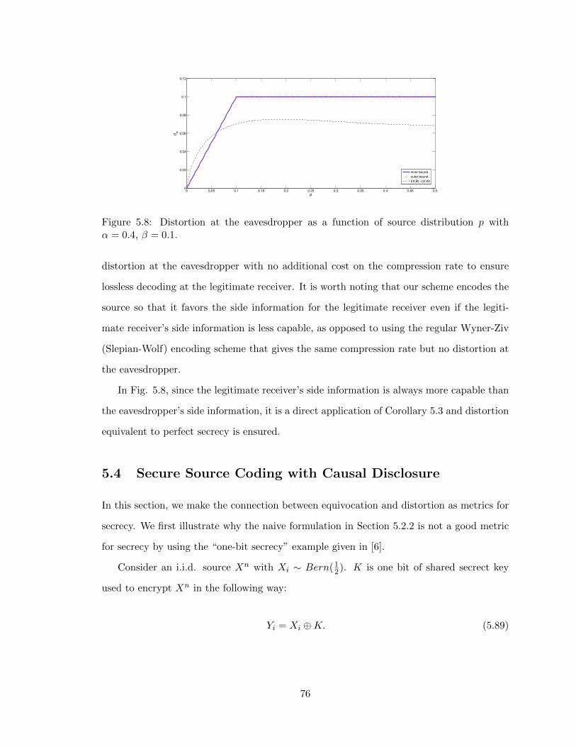
0 0.05 0.1 0.15 0.2 0.25 0.3 0.35 0.4 0.45 0.50
0.02
0.04
0.06
0.08
0.1
0.12
p
dw
inner bound
outer bound
I(X;B)−I(X;W)
Figure 5.8: Distortion at the eavesdropper as a function of source distribution p withα = 0.4, β = 0.1.
distortion at the eavesdropper with no additional cost on the compression rate to ensure
lossless decoding at the legitimate receiver. It is worth noting that our scheme encodes the
source so that it favors the side information for the legitimate receiver even if the legiti-
mate receiver’s side information is less capable, as opposed to using the regular Wyner-Ziv
(Slepian-Wolf) encoding scheme that gives the same compression rate but no distortion at
the eavesdropper.
In Fig. 5.8, since the legitimate receiver’s side information is always more capable than
the eavesdropper’s side information, it is a direct application of Corollary 5.3 and distortion
equivalent to perfect secrecy is ensured.
5.4 Secure Source Coding with Causal Disclosure
In this section, we make the connection between equivocation and distortion as metrics for
secrecy. We first illustrate why the naive formulation in Section 5.2.2 is not a good metric
for secrecy by using the “one-bit secrecy” example given in [6].
Consider an i.i.d. source Xn with Xi ∼ Bern(12). K is one bit of shared secrect key
used to encrypt Xn in the following way:
Yi = Xi ⊕K. (5.89)
76
Upon receiving Y n the legitimate receiver can decode with the shared secret key K. Under
Hamming distortion, it is easy to see that the eavesdropper’s best strategy is to output
Zn = Y n, yielding an average distortion of 12 . This is indeed the maximum possible average
distortion. However, this is a vulnerable secrecy model because the eavesdropper knows
that Xn can only be one of the two candidate sequences.
In the above example, the eavesdropper is able to decode the entire sequence accurately
after observing the first symbol realization. Motivated by this observation, [4] [5] and
[6] formulate the rate-distortion based secrecy setting with causal disclosure, where the
eavesdropper has access to the past realization of the source sequence. It is also shown in
[6] that the equivocation metric becomes a special case of the distortion metric with causal
source disclosure by choosing the distortion function to be log-loss. Here we recap the main
result under this setting.
5.4.1 Problem Formulation
We want to determine the rate-distortion region for a secrecy system with an i.i.d. source
sequence Xn distributed according to∏nt=1 PX(xt) satisfying the following constraints:
• Encoder fn : X n ×K 7→M (possibly stochastic)
• Legitimate receiver decoder gn :M×K 7→ Yn (possibly stochastic)
• Eavesdropper decoder {PZt|MXt−1}nt=1
• Compression rate: R, i.e. |M| = 2nR
• Secret key rate: R0, i.e. |K| = 2nR0 .
The system performance is measured according to the following distortion metrics:
• Average distortion for the legitimate receiver:
lim supn→∞
E [db(Xn, Y n)] ≤ Db (5.90)
77
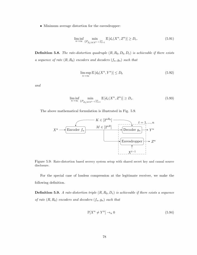
• Minimum average distortion for the eavesdropper:
lim infn→∞
min{PZt|MXt−1}nt=1
E [de(Xn, Zn)] ≥ De. (5.91)
Definition 5.8. The rate-distortion quadruple (R,R0, Db, De) is achievable if there exists
a sequence of rate (R,R0) encoders and decoders (fn, gn) such that
lim supn→∞
E [db(Xn, Y n)] ≤ Db (5.92)
and
lim infn→∞
min{PZt|MXt−1}nt=1
E [de(Xn, Zn)] ≥ De. (5.93)
The above mathematical formulation is illustrated in Fig. 5.9.
Xn Encoder fn Decoder gn Y n
K ∈ [2nR0 ]
Eavesdropper Zn
Xt−1
t = 1, ..., n
M ∈ [2nR]
Figure 5.9: Rate-distortion based secrecy system setup with shared secret key and causal sourcedisclosure.
For the special case of lossless compression at the legitimate receiver, we make the
following definition.
Definition 5.9. A rate-distortion triple (R,R0, De) is achievable if there exists a sequence
of rate (R,R0) encoders and decoders (fn, gn) such that
P[Xn 6= Y n]→n 0 (5.94)
78

and
lim infn→∞
min{PZt|MXt−1}nt=1
E [de(Xn, Zn)] ≥ De. (5.95)
5.4.2 Main Results
The main results are summarized in the following theorem. The proofs are found in the
original paper [6] and not presented here.
Theorem 5.6. The rate-distortion quadruple (R,R0, Db, De) is achievable if and only if
R ≥ I(X;Y ) (5.96)
R0 ≥ I(X;Y |U) (5.97)
Db ≥ E[db(X,φ(Y ))] (5.98)
De ≤ minz(u)
E[de(X, z(U))] (5.99)
for some distribution PXPY |XPU |Y and some function φ(·).
For the special case of lossless compression, we have the following corollary.
Corollary 5.4. The rate-distortion triple (R,R0, De) is achievable if and only if
R ≥ H(X) (5.100)
R0 ≥ H(X|U) (5.101)
De ≤ minz(u)
E[de(X, z(U))] (5.102)
for some distribution PXPU |X .
5.4.3 Equivocation
We now examine Theorem 5.6 by setting de(·, ·) to the log-loss function defined as
de(x, z) = log1
z(x)(5.103)
79
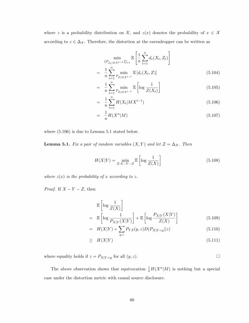
where z is a probability distribution on X , and z(x) denotes the probability of x ∈ X
according to z ∈ ∆X . Therefore, the distortion at the eavesdropper can be written as
min{PZt|MXt−1}nt=1
E
[1
n
n∑t=1
de(Xt, Zt)
]
=1
n
n∑t=1
minPZ|MXt−1
E [de(Xt, Z)] (5.104)
=1
n
n∑t=1
minPZ|MXt−1
E[log
1
Z(Xt)
](5.105)
=1
n
n∑t=1
H(Xt|MXt−1) (5.106)
=1
nH(Xn|M) (5.107)
where (5.106) is due to Lemma 5.1 stated below.
Lemma 5.1. Fix a pair of random variables (X,Y ) and let Z = ∆X . Then
H(X|Y ) = minZ:X−Y−Z
E[log
1
Z(X)
](5.108)
where z(x) is the probability of x according to z.
Proof. If X − Y − Z, then
E[log
1
Z(X)
]= E
[log
1
PX|Y (X|Y )
]+ E
[log
PX|Y (X|Y )
Z(X)
](5.109)
= H(X|Y ) +∑y,z
PY Z(y, z)D(PX|Y=y||z) (5.110)
≥ H(X|Y ) (5.111)
where equality holds if z = PX|Y=y for all (y, z).
The above observation shows that equivocation 1nH(Xn|M) is nothing but a special
case under the distortion metric with causal source disclosure.
80
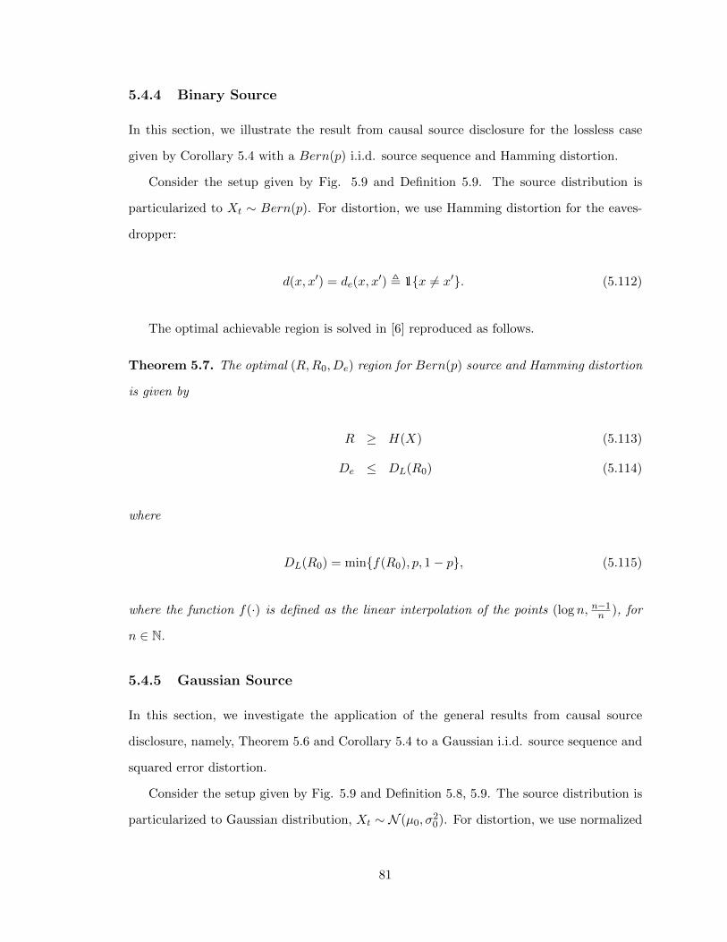
5.4.4 Binary Source
In this section, we illustrate the result from causal source disclosure for the lossless case
given by Corollary 5.4 with a Bern(p) i.i.d. source sequence and Hamming distortion.
Consider the setup given by Fig. 5.9 and Definition 5.9. The source distribution is
particularized to Xt ∼ Bern(p). For distortion, we use Hamming distortion for the eaves-
dropper:
d(x, x′) = de(x, x′) , 1{x 6= x′}. (5.112)
The optimal achievable region is solved in [6] reproduced as follows.
Theorem 5.7. The optimal (R,R0, De) region for Bern(p) source and Hamming distortion
is given by
R ≥ H(X) (5.113)
De ≤ DL(R0) (5.114)
where
DL(R0) = min{f(R0), p, 1− p}, (5.115)
where the function f(·) is defined as the linear interpolation of the points (log n, n−1n ), for
n ∈ N.
5.4.5 Gaussian Source
In this section, we investigate the application of the general results from causal source
disclosure, namely, Theorem 5.6 and Corollary 5.4 to a Gaussian i.i.d. source sequence and
squared error distortion.
Consider the setup given by Fig. 5.9 and Definition 5.8, 5.9. The source distribution is
particularized to Gaussian distribution, Xt ∼ N (µ0, σ20). For distortion, we use normalized
81
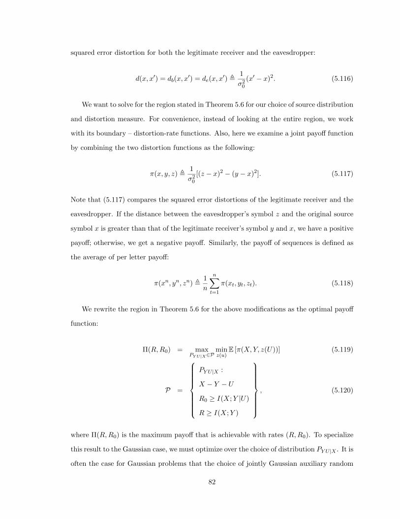
squared error distortion for both the legitimate receiver and the eavesdropper:
d(x, x′) = db(x, x′) = de(x, x
′) ,1
σ20
(x′ − x)2. (5.116)
We want to solve for the region stated in Theorem 5.6 for our choice of source distribution
and distortion measure. For convenience, instead of looking at the entire region, we work
with its boundary – distortion-rate functions. Also, here we examine a joint payoff function
by combining the two distortion functions as the following:
π(x, y, z) ,1
σ20
[(z − x)2 − (y − x)2]. (5.117)
Note that (5.117) compares the squared error distortions of the legitimate receiver and the
eavesdropper. If the distance between the eavesdropper’s symbol z and the original source
symbol x is greater than that of the legitimate receiver’s symbol y and x, we have a positive
payoff; otherwise, we get a negative payoff. Similarly, the payoff of sequences is defined as
the average of per letter payoff:
π(xn, yn, zn) ,1
n
n∑t=1
π(xt, yt, zt). (5.118)
We rewrite the region in Theorem 5.6 for the above modifications as the optimal payoff
function:
Π(R,R0) = maxPY U|X∈P
minz(u)
E [π(X,Y, z(U))] (5.119)
P =
PY U |X :
X − Y − U
R0 ≥ I(X;Y |U)
R ≥ I(X;Y )
, (5.120)
where Π(R,R0) is the maximum payoff that is achievable with rates (R,R0). To specialize
this result to the Gaussian case, we must optimize over the choice of distribution PY U |X . It is
often the case for Gaussian problems that the choice of jointly Gaussian auxiliary random
82
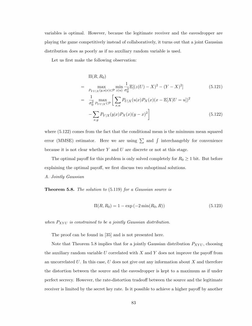
variables is optimal. However, because the legitimate receiver and the eavesdropper are
playing the game competitively instead of collaboratively, it turns out that a joint Gaussian
distribution does as poorly as if no auxiliary random variable is used.
Let us first make the following observation:
Π(R,R0)
= maxPY U|X(y,u|x)∈P
minz(u)
1
σ20
E[(z(U)−X)2 − (Y −X)2] (5.121)
=1
σ20
maxPY U|X∈P
[∑x,u
PU |X(u|x)PX(x)(x− E[X|U = u])2
−∑x,y
PY |X(y|x)PX(x)(y − x)2
](5.122)
where (5.122) comes from the fact that the conditional mean is the minimum mean squared
error (MMSE) estimator. Here we are using∑
and∫
interchangebly for convenience
because it is not clear whether Y and U are discrete or not at this stage.
The optimal payoff for this problem is only solved completely for R0 ≥ 1 bit. But before
explaining the optimal payoff, we first discuss two suboptimal solutions.
A. Jointly Gaussian
Theorem 5.8. The solution to (5.119) for a Gaussian source is
Π(R,R0) = 1− exp (−2 min(R0, R)) (5.123)
when PXY U is constrained to be a jointly Gaussian distribution.
The proof can be found in [35] and is not presented here.
Note that Theorem 5.8 implies that for a jointly Gaussian distribution PXY U , choosing
the auxiliary random variable U correlated with X and Y does not improve the payoff from
an uncorrelated U . In this case, U does not give out any information about X and therefore
the distortion between the source and the eavesdropper is kept to a maximum as if under
perfect secrecy. However, the rate-distortion tradeoff between the source and the legitimate
receiver is limited by the secret key rate. Is it possible to achieve a higher payoff by another
83
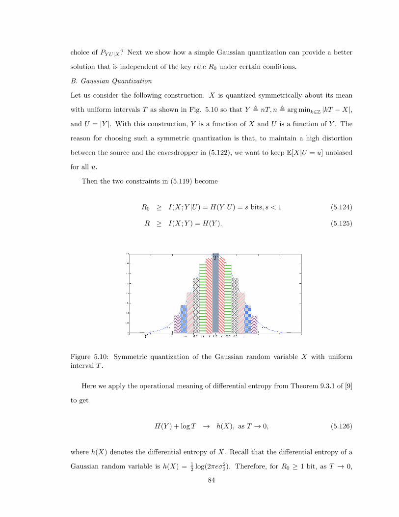
choice of PY U |X? Next we show how a simple Gaussian quantization can provide a better
solution that is independent of the key rate R0 under certain conditions.
B. Gaussian Quantization
Let us consider the following construction. X is quantized symmetrically about its mean
with uniform intervals T as shown in Fig. 5.10 so that Y , nT, n , arg mink∈Z |kT −X|,
and U = |Y |. With this construction, Y is a function of X and U is a function of Y . The
reason for choosing such a symmetric quantization is that, to maintain a high distortion
between the source and the eavesdropper in (5.122), we want to keep E[X|U = u] unbiased
for all u.
Then the two constraints in (5.119) become
R0 ≥ I(X;Y |U) = H(Y |U) = s bits, s < 1 (5.124)
R ≥ I(X;Y ) = H(Y ). (5.125)
Figure 5.10: Symmetric quantization of the Gaussian random variable X with uniforminterval T .
Here we apply the operational meaning of differential entropy from Theorem 9.3.1 of [9]
to get
H(Y ) + log T → h(X), as T → 0, (5.126)
where h(X) denotes the differential entropy of X. Recall that the differential entropy of a
Gaussian random variable is h(X) = 12 log(2πeσ2
0). Therefore, for R0 ≥ 1 bit, as T → 0,
84

a sufficient condition for (5.125) is T ≥√
2πeσ0 exp(−R). The distortion between the
source and the eavesdropper under this Gaussian quantization scheme can be asymptotically
calculated as follows:
D∆(R) =
∫ ∞−∞
∑y
PY |X(y|x)1√
2πσ0
e− x2
2σ20 (y − x)2dx (5.127)
=
∫ ∞−∞
1√2πσ0
e− x2
2σ20 (nT − x)2dx (5.128)
≤ πe
2σ2
0 exp(−2R). (5.129)
Summarizing the above analysis, we have
Π(R,R0) ≥ 1− πe
22−2R for R0 ≥ 1 bit and R→∞. (5.130)
With Gaussian quantization, even though we sacrifice a constant factor on the distortion
between the source and the legitimate receiver, the overall payoff is no longer governed by
the key rate R0 given that R0 ≥ 1 bit. This illustrates that the joint Gaussian distribution
does not achieve optimal payoff. Next, we provide a construction for Y and U that achieves
maximum payoff under certain conditions.
Optimal Payoff for R0 ≥ 1 bit
Theorem 5.9. If the key rate R0 ≥ 1 bit, the optimal secrecy rate-payoff function for an
i.i.d. Gaussian source is given by
Π(R,R0) = 1− 2−2R. (5.131)
Proof. To see the converse, observe that by relaxing the constraints in (5.119) and evaluating
(5.122), we have
maxPY U|X
∑u,x
PU |X(u|x)PX(x)(x− E[X|U = u])2 = σ20 (5.132)
minPY U|X :I(X;Y )≤R
∑x,y
PY |X(y|x)PX(x)(y − x)2 = σ202−2R (5.133)
85

where (5.133) comes from the distortion rate function d(R) of a Gaussian source. To show
the achievability, we choose PY U |X as follows. Y is chosen such that X and Y are zero-mean
jointly Gaussian. U , |Y | and V , sgn(Y ), where sgn(Y ) is a binary variable indicating
the sign of Y . Observe that U, V together gives Y . By this construction, we have
I(X;Y |U) = I(X;V |U) < 1 bit. (5.134)
Therefore, given that R0 ≥ 1 bit, the constraint R0 ≥ I(X;Y |U) is automatically satisfied
from (5.134). In addition, E[X|U = u] = 12E[X|Y = u] + 1
2E[X|Y = −u] = 0 for all u due
to symmetry. The payoff achieves 1− 2−2R.
The optimization problem (5.119) for the case R0 < 1 bit involves the coupling of two
terms in (5.122). We next present a special case for this regime using a Gaussian quantizer.
Gaussian Quantizer Special Case
We now address a special structure of the system with causal source disclosure. A symbol-
by-symbol quantization of the source sequence is performed before the transmission and
the legitimate receiver in this system happens to reproduce the scalar quantization of the
source at the decoder. That is, we are restricting to a subset Bn of all valid encoder and
decoder pairs (fn, gn).
Let Xt ∼ p0 be the conditional mean of a uniform quantization of Xt as in Fig. 5.10,
i.e. Xt = E[Xt|Quantization bin of Xt], and M be the encoded message to be transmitted.
Let the optimal payoff function under such restriction be Π∆(R,R0). The following lemma
indicates that revealing the causal realization of the original source is equivalent to revealing
the causal realization of the quantized version of the source in the eavesdropper’s estimate.
Lemma 5.2.
Xt − (M, Xt−1)−Xt−1 (5.135)
for all t = 1, ..., n.
86
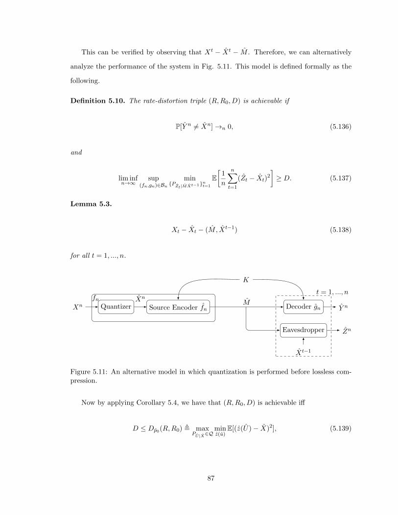
This can be verified by observing that Xt − Xt − M . Therefore, we can alternatively
analyze the performance of the system in Fig. 5.11. This model is defined formally as the
following.
Definition 5.10. The rate-distortion triple (R,R0, D) is achievable if
P[Y n 6= Xn]→n 0, (5.136)
and
lim infn→∞
sup(fn,gn)∈Bn
min{PZt|MXt−1}nt=1
E[
1
n
n∑t=1
(Zt − Xt)2
]≥ D. (5.137)
Lemma 5.3.
Xt − Xt − (M, Xt−1) (5.138)
for all t = 1, ..., n.
Xn Quantizer Source Encoder fn Decoder gn Y n
K
Xnfnt = 1, ..., n
Eavesdropper Zn
Xt−1
M
Figure 5.11: An alternative model in which quantization is performed before lossless com-pression.
Now by applying Corollary 5.4, we have that (R,R0, D) is achievable iff
D ≤ Dp0(R,R0) , maxPU|X∈Q
minz(u)
E[(z(U)− X)2], (5.139)
87
where X ∼ p0 and
Q = {PU |X : R ≥ H(X), R0 ≥ H(X|U)}. (5.140)
If we fix (R,R0) and suppose PU |X ∈ Q is the corresponding distribution that achieves
Dp0(R,R0),
Zn , {PZt|MXt−1}nt=1, (5.141)
Zn , {PZt|MXt−1}nt=1, (5.142)
then we have the following inequalities:
σ20Π∆(R,R0)
= limn→∞
supBn
minZn
1
n
n∑t=1
E[(Zt −Xt)2]− E[(Xt − Yt)2] (5.143)
= limn→∞
supBn
minZn
1
n
n∑t=1
E[(Zt −Xt)2]− E[(Xt − Yt)2] (5.144)
= limn→∞
supBn
minZn
1
n
n∑t=1
E[(Zt − Xt)2] + E[(Xt −Xt)
2]
+2E[E[(Zt − Xt)(Xt −Xt)|Xt]
]− E[(Xt − Yt)2] (5.145)
= limn→∞
supBn
minZn
1
n
n∑t=1
E[(Zt − Xt)2] +
1
n
n∑t=1
E[(Xt −Xt)2]− E[(Xt − Yt)2](5.146)
= Dp0(R,R0). (5.147)
Here, (5.143) follows by definition of Π∆(R,R0); (5.144) follows from Lemma 5.2; (5.145)
follows from law of total expectation; (5.146) follows from Lemma 5.3; and (5.147) follows
by Definition 5.10. Summarizing the analysis in this section, we have the following theorem.
Theorem 5.10. Π∆(R,R0) = 1σ2
0Dp0(R,R0).
Dp0(R,R0) can be calculated as a linear program (LP).
88
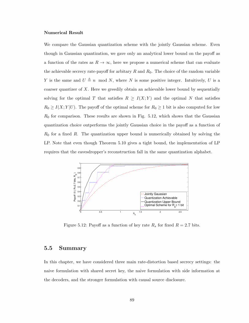
Numerical Result
We compare the Gaussian quantization scheme with the jointly Gaussian scheme. Even
though in Gaussian quantization, we gave only an analytical lower bound on the payoff as
a function of the rates as R → ∞, here we propose a numerical scheme that can evaluate
the achievable secrecy rate-payoff for arbitary R and R0. The choice of the random variable
Y is the same and U , n mod N , where N is some positive integer. Intuitively, U is a
coarser quantizer of X. Here we greedily obtain an achievable lower bound by sequentially
solving for the optimal T that satisfies R ≥ I(X;Y ) and the optimal N that satisfies
R0 ≥ I(X;Y |U). The payoff of the optimal scheme for R0 ≥ 1 bit is also computed for low
R0 for comparison. These results are shown in Fig. 5.12, which shows that the Gaussian
quantization choice outperforms the jointly Gaussian choice in the payoff as a function of
R0 for a fixed R. The quantization upper bound is numerically obtained by solving the
LP. Note that even though Theorem 5.10 gives a tight bound, the implementation of LP
requires that the eavesdropper’s reconstruction fall in the same quantization alphabet.
0 0.5 1 1.5 2 2.50
0.1
0.2
0.3
0.4
0.5
0.6
0.7
0.8
0.9
1
RS
Payoff Π
( R
=2.7
bits, R
S )
Jointly Gaussian
Quantization Achievable
Quantization Upper BoundOptimal Scheme for R
s≥ 1 bit
Figure 5.12: Payoff as a function of key rate Rs for fixed R = 2.7 bits.
5.5 Summary
In this chapter, we have considered three main rate-distortion based secrecy settings: the
naive formulation with shared secret key, the naive formulation with side information at
the decoders, and the stronger formulation with causal source disclosure.
89

For the naive formulation with shared secret key, the problem has been solved com-
pletely: a secret key of a positive rate is necessary and sufficient to force the maximum
possible distortion to the eavesdropper.
For the naive formulation with side information at decoders, we have obtained an inner
and an outer bound. The results show that even if the legitimate receiver has a weaker side
information, a positive distortion can still be enforced to the eavesdropper with a proper
encoding. Although exact bounds have been obtained for several special cases, the outer
bound for arbitrarily correlated side information is not tight, which suggests an interesting
direction for future work.
For the stronger formulation with causal source disclosure, the general result is com-
plete. Its relation to equivocation has been discussed and it has been proved mathematically
that equivocation is a special case of the rate-distortion approach. Two examples of com-
mon sources and distortion metrics, binary source under Hamming distortion and Gaussian
source under squared error distortion, have been studied in detail.
90
Chapter 6
Source-Channel Security in the
Noisy Wiretap Channel
6.1 Introduction
Unlike the point-to-point communication system, separating the encodings of source com-
pression and channel coding is in general not optimal in a multi-terminal setting. Building
upon the secrecy models proposed in Chapter 5, we extend them to joint source-channel
settings by allowing noisy channels.
In this chapter, we start by considering operationally separate source-channel coding
in the context of secrecy. It turns out for the naive secrecy formulation, operationally
separate source-channel coding is optimal. However, under the strong formulation, where
the source is causally disclosed to the eavesdropper during decoding, separation does not
hold. This motivates us to explore more efficient ways of conducting source-channel coding.
Recent work [8] on hybrid coding provides a new approach for joint source-channel coding.
Furthermore, the analysis of hybrid coding aligns nicely with the likelihood encoder.
91

6.2 Operational Separate Source-Channel Security
6.2.1 Naive Formulation
Problem Setup
A source node has an independent and i.i.d. sequence Sk that it intends to transmit over
a memoryless broadcast channel PY Z|X such that a legitimate receiver can reliably decode
the source sequence, while keeping the distortion between an eavesdropper and the source
as high as possible. The source sequence Sk is mapped to the channel input sequence Xn
through a source-channel encoder. Upon receiving Y n, the legitimate receiver makes an
estimate Sk of the original source sequence Sk. Similarly, the eavesdropper also makes an
estimate Sk of Sk upon receiving Zn.
The input of the system is an i.i.d. source sequence Sk distributed according to∏kj=1 PS(sj) and the channel is a memoryless broadcast channel
∏nt=1 PY Z|X(yt, zt|xt). The
source-channel coding model satisfies the following constraints:
• Encoder fk,n : Sk 7→ X n (possibly stochastic);
• Legitimate receiver decoder gk,n : Yn 7→ Sk (possibly stochastic);
• Eavesdropper decoders PSk|Zn ;
• Communication rate: R = kn , i.e. symbol/channel use.
The system performance is measured by the error probability at the legitimate receiver and
a distortion metric d(·, ·) at the eavesdropper as follows:
• Lossless compression for the legitimate receiver:
P[Sk 6= Sk
]→k 0 (6.1)
• Minimum average distortion for the eavesdropper:
lim infk→∞
minPSk|Zn
E[d(Sk, Sk)] ≥ D. (6.2)
92

Definition 6.1. For a given distortion function d(·, ·), a rate distortion pair (R,D) is
achievable if there exists a sequence of encoder and decoder pairs (fk,n, gk,n) such that
k
n= R,
P[Sk 6= Sk
]→k 0,
and
lim infk→∞
minPSk|Zn
E[d(Sk, Sk)
]≥ D.
Note that the rate-distortion pair (R,D) captures the tradeoff between the communica-
tion rate for reliable transmission and the eavesdropper’s distortion, which is different from
rate-distortion theory in the traditional sense.
The above mathematical formulation is illustrated in Fig. 6.7.
The average distortion achieved by guesses based only on the prior distribution of the
source ∆, is defined as
∆ , mina
E[d(S, a)]. (6.3)
Encoder fk,n PY Z|X
Decoder gk,n
Eavesdropper
Sk XnY n
Zn
Sk
Sk
Figure 6.1: Source-channel secrecy system setup at the eavesdropper.
Main Results
We first make some general observations about the communication between the transmitter
and the legitimate receiver, as well as the communication between the transmitter and the
eavesdropper. If the eavesdropper is not present, the transmitter and receiver can commu-
nicate losslessly at any rate lower than R0 ,maxX I(X;Y )
H(S) because separate source-channel
coding is optimal for point-to-point communication. Ideally, we want to force maximum
93
average distortion ∆ upon the eavesdropper. But higher distortion to the eavesdropper may
come at the price of a lower communication rate to the legitimate receiver.
As for physical layer secrecy of a memoryless broadcast channel, the result for trans-
mitting two messages, one confidential and one public, from Csiszar and Korner [30] has
been known for many decades. In their work, weak secrecy was considered. This result
was strengthened in [36] by considering strong secrecy. The same rate region was obtained
in [36], however the metric for secrecy is stronger. In our work, the source-channel coding
schemes we propose operationally separate source and channel coding that requires dividing
the bit sequence produced by source coding into two messages which are then processed by
the channel coding. The channel coding part functions in a way that is similar to [30] or
[36], except that the public message in those works is not required to be decoded in our
case, and we refer to that message as the “non-confidential” message.
We now state the rate-distortion result for general source-channel coding with an i.i.d.
source sequence and a discrete memoryless broadcast channel PY Z|X . In the following
theorem, we will see that the source sequence can be delivered almost losslessly to the
legitimate receiver at a rate arbitarily close to R0 while the distortion to the eavesdropper
is kept at ∆, as long as the secrecy capacity is positive.
Theorem 6.1. For an i.i.d. source sequence Sk and memoryless broadcast channel PY Z|X ,
if there exists W −X − Y Z such that I(W ;Y )− I(W ;Z) > 0, then (R,D) is achievable if
and only if
R <maxX I(X;Y )
H(S), (6.4)
D ≤ ∆, (6.5)
where ∆ was defined in (6.3).
Remark: The requirement I(W ;Y ) − I(W ;Z) > 0 implies the existence of a secure
channel with a positive rate, i.e. the eavesdropper’s channel is not less noisy than the in-
tended receiver’s channel. So instead of demanding a high secure transmission rate with
perfect secrecy to accommodate the description of the source, we need only to ensure the
94

existence of a secure channel with positive rate. This will suffice to ensure that the eaves-
dropper’s distortion is maximal.
The converse is straightforward. Each of the inequalities (6.4) and (6.5) is true indi-
vidually for any channel and source, (6.4) by channel capacity coupled by optimality of
source-channel separation, and (6.5) by definition.
Achievability
The idea for achievability is to operationally separate the source and channel coding (see
Fig. 6.2). The source encoder compresses the source and splits the resulting message into
a confidential message and a non-confidential message. A channel encoder is concatenated
digitally with the source encoder so that the channel delivers both the confidential and non-
confidential messages reliably to the legitimate receiver and keeps the confidential message
secret from the eavesdropper, as in [30]. The overall source-channel coding rate will have
the following form: R = kn = k
log |M| ·log |M|n = Rch
Rsrc, where |M| is the total cardinality of
the confidential and the non-confidential messages; Rch and Rsrc are the channel coding
and source coding rates, respectively.
Let us look at two models that will help us establish the platform for showing the
achievability of Theorem 6.1.
fcfs PY Z|X
Decoder gk,n
Eavesdropper
Sk Mp
Ms
XnY n
Zn
Sk
Sk
Figure 6.2: Operationally separate source-channel coding: the confidential and non-confidential messages satisfy Ms ∈ [1 : 2kR
′s = 2nRs ] and Mp ∈ [1 : 2kR
′p = 2nRp ].
A. Channel Coding and Strong Secrecy
Consider a memoryless broadcast channel PY Z|X and a communication system with a
confidential message Ms and a non-confidential message Mp that must allow the intended
receiver to decode both Ms and Mp while keeping the eavesdropper from learning anything
about Ms. Problems like this were first studied by Csiszar and Korner [30] in 1978, as
an extension of Wyner’s work in [7]. However, their model and our model differ in that
95
the second receiver in their setting is required to decode the public message Mp. The
mathematical formulation and result of our channel model is stated below. We focus on the
message pairs (Ms,Mp) whose distribution satisfies the following:
PMs|Mp=mp(ms) = 2−nRs (6.6)
for all (ms,mp). Later we will show that a source encoder can always prepare the input
messages to the channel in this form.
Definition 6.2. An (Rs, Rp, n) channel code consists of a channel encoder fc (possibly
stochastic) and a channel decoder gc such that
fc :Ms ×Mp 7→ X n
and
gc : Yn 7→ Ms ×Mp
where |Ms| = 2nRs and |Mp| = 2nRp.
Definition 6.3. The rate pair (Rs, Rp) is achievable under weak secrecy if for all (Ms,Mp)
satisfying (6.6), there exists a sequence of (Rs, Rp, n) channel codes such that
P[(Ms,Mp) 6= (Ms, Mp)
]→n 0 (6.7)
and
1
nI(Ms;Z
n|Mp)→n 0. (6.8)
Note that because the eavesdropper may completely or partially decode Mp, the secrecy
requirement is modified accordingly to consider I(Ms;Zn|Mp) instead of I(Ms;Z
n). To
guarantee true secrecy of Ms, we want to make sure that even if Mp is given to the eaves-
dropper, there is no information leakage of Ms, because I(Ms;Zn|Mp) = I(Ms;Z
nMp) if
Ms and Mp are independent.
96
Theorem 6.2. A rate pair (Rs, Rp) is achievable under weak secrecy if
Rs ≤ I(W ;Y |V )− I(W ;Z|V ), (6.9)
Rp ≤ I(V ;Y ) (6.10)
for some V −W −X − Y Z.
The proof is given in Appendix 6.5.5. Let us denote the above region as R. We now
strengthen the result by considering strong secrecy introduced in [37]. Later we will use
strong secrecy to connect the operationally separate source and channel encoders.
Definition 6.4. The rate pair (Rs, Rp) is achievable under strong secrecy if for all
(Ms,Mp) satisfying (6.6), there exists a sequence of (Rs, Rp, n) channel codes such that
P[(Mp,Ms) 6= (Ms, Mp)]→n 0 (6.11)
and
I(Ms;Zn|Mp)→n 0. (6.12)
In general, weak secrecy does not necessarily imply that strong secrecy is also achievable;
however, in this particular setting we have the following claim:
Theorem 6.3. A rate pair (Rs, Rp) achievable under weak secrecy is also achievable under
strong secrecy.
The following two lemmas will assist the proof of Theorem 6.3 by providing a sufficient
condition for satisfying the secrecy constraint I(Ms;Zn|Mp)→n 0.
Lemma 6.1. If
∥∥PZn|Mp=mpPMs|Mp=mp − PZnMs|Mp=mp
∥∥TV≤ ε ≤ 1
2, (6.13)
97
then
I(Ms;Zn|Mp = mp) ≤ −ε log
ε
|Ms|. (6.14)
The proof of Lemma 6.1 is provided in Appendix 6.5.1.
Lemma 6.2. If for every (ms,mp), there exists a measure θmp on Zn such that
∥∥PZn|Mp=mpMs=ms − θmp∥∥TV≤ εn (6.15)
then
I(Ms;Zn|Mp)→n 0 (6.16)
where εn = 2−nβ for some β > 0.
A proof of Lemma 6.2 is given in Appendix 6.5.2.
If there exist channel codes such that P[(Ms,Mp) 6= (Ms, Mp)
]→n 0 and measure θmp
for all (ms,mp) such that ||PZn|Mp=mpMs=ms − θmp ||TV ≤ εn, then Theorem 6.3 follows
immediately. The existence of such a code and measure is assured by the same codebook
construction and choice of measure as in [36].
B. Source Coding
Here we consider a source coding model in which the transmitter has an i.i.d. source
sequence Sk. A source encoder is needed to prepare Sk by encoding it into a pair of
messages (Ms,Mp) that satisfies PMs|Mp=mp(ms) = 2−kR′s = 2−nRs . Note that this condition
is enforced only for the purpose of channel coding so that the messages generated by the
source encoder satisfy (6.6) to be a valid channel input.
Definition 6.5. An (R′s, R′p, k) source code consists of an encoder fs and a decoder gs such
that
fs : Sk 7→ Ms ×Mp
gs :Ms ×Mp 7→ Sk
98
where |Ms| = 2kR′s and |Mp| = 2kR
′p.
Definition 6.6. A rate distortion triple (R′s, R′p, D) is achievable under a given distortion
measure d(·, ·) if there exists a sequence of (R′s, R′p, k) source codes such that
P[Sk 6= gs(fs(S
k))]→k 0 (6.17)
and the message pair generated by the source encoder satisfies PMs|Mp=mp(ms) = 2−kR′s and
for all PZn|MsMpsuch that I(Ms;Z
n|Mp)→n 0
lim infk→∞
minsk(zn)
E[d(Sk, sk(Zn))
]≥ D. (6.18)
Theorem 6.4. (R′s, R′p, D) is achievable if
R′s > 0, (6.19)
R′s +R′p > H(S), (6.20)
and
D ≤ ∆. (6.21)
The general idea for achievability is to consider the ε-typical Sk sequences and partition
them into bins of equal size so that each bin contains sequences of the same type. The
identity Mp of the bin is revealed to all parties, but the identity Ms of each sequence inside
a bin is perfectly protected.1 Each such partition is treated as a codebook. It was shown
in [3] that, for the noiseless case in which the eavesdropper is given mp instead of zn, the
distortion averaged over all such codebooks achieves the maximum average distortion ∆ as
k →∞ and therefore there must exist one partition that achieves ∆. In order to transition
1Strictly speaking, the source encoder may violate the condition (6.6) on (k + 1)|S| number of bins,because (k+ 1)|S| is an upper bound on the number of types of a sequence of length k. However, this is justa very small (polynomial in k) number of bins compared with the total number (roughly 2kH(S)) of bins.Therefore, for this small portion of “bad” bins that violate (6.6), we can just let the source encoder declarean error on the confidential message Ms and construct a dummy Ms uniformly given the bin index mp. Thiswill contribute only an ε factor to the error probability.
99
from the result in [3] to our claim in Theorem 6.4, we only need to show
minsk(zn)
E[dk(Sk, sk(Zn))
]≥ min
sk(mp)E[dk(Sk, sk(Mp))
]− 2δ′(ε). (6.22)
Proof. First, observe that
minsk(·)
E[dk(Sk, sk(·))
]=
1
k
k∑i=1
mins(i,·)
E [d(Si, s(i, ·))] . (6.23)
Next, we claim the channel output sequence zn does not provide the eavesdropper any-
thing more than mp and therefore
mins(i,zn)
E
[1
k
k∑i=1
d(Si, s(i, Zn))
]≥ min
s(i,mp)E
[1
k
k∑i=1
d(Si, s(i,Mp))
]− 2δ′(ε). (6.24)
The analysis is similar to that in [38], but for the sake of clarity, we present the complete
proof of (6.24) in Appendix 6.5.3. Here strong secrecy comes into play. It is also pointed
out within the proof in Appendix 6.5.3 that I(Ms;Zn|Mp)→n 0 is needed.
Finally, combining (6.24) with (6.23) gives us the desired result.
C. Achievability Proof of Theorem 6.1
We are now ready to complete the achievability proof of Theorem 6.1 using Theorems 6.2
and Theorem 6.4 by concatenating the channel encoder with the source encoder.
Fix ν ≥ ε > 0. Fix PS . Let Rs′ = 2ν, Rp
′ = H(S) − ν and R′ = Rs′ + Rp
′. We
apply the same codebook construction and encoding scheme as in B by partioning the ε-
typical Sk sequences into 2kRp′
bins and inside each bin we have 2kRs′
sequences so that
P[Sk 6= gs(fs(Sk))] ≤ ε. Recall that all the sequences inside one bin are of the same type,
so it is guaranteed that
PMs|Mp=mp(ms) =1
|Ms|=
1
2kR′s(6.25)
for all mp, ms, which implies I(Ms;Mp) = 0.
100

Let Rs and Rp be the channel rates. Rp is seen as a function of Rs on the boundary of the
region given in Theorem 6.2 and this is denoted by Rp(Rs). Suppose max(Rs,Rp)∈RRs > 0,
i.e. there exists W−X−Y Z such that I(W ;Y )−I(W ;Z) > 0 (justified in Appendix 6.5.4).
Rp(Rs) is continuous and non-increasing. Thus, Rp achieves its maximum at Rs = 0, which
would be the channel capacity maxX I(X;Y ) of PY |X for reliable transmission. By the
continuity of Rp(Rs), (Rs, Rp) = (2ν kn , Rp(0)− δ(ν)) is achievable under strong secrecy, i.e.
P[(Ms,Mp) 6= (Ms, Mp)] ≤ ε and I(Ms;Zn|Mp) ≤ ε, where δ(ν)→ 0 as ν → 0.
From the above good channel code under strong secrecy we have PZn|MsMpsuch that
I(Ms;Zn|Mp)→n 0. Therefore, we can apply Theorem 6.4 to achieve
minsk(zn)
E[dk(Sk, sk(Zn))
]→k D. (6.26)
The error probability is bounded by the sum of the error probabilities from the source
coding and channel coding parts, i.e. P[Sk 6= Sk
]< 2ε. Finally, we verify the total
transmission rate to complete the proof:
R =k
n=Rs +RpR′s +R′p
(6.27)
=Rp(0)− δ(ν) + 2Rν
H(S) + ν(6.28)
≥ Rp(0)− δ(ν)
H(S) + ν(6.29)
ν→0−→ maxX I(X;Y )
H(S). (6.30)
6.2.2 With Causal Source Disclosure at the Eavesdropper
Problem Setup
Now we consider a variation of the problem considered in Section 6.2.1. We want to deter-
mine conditions for a joint source-channel secrecy system that guarantee reliable commu-
nication to the legitimate receiver while a certain level of distortion can be forced on the
eavesdropper. The input of the system is an i.i.d. source sequence Sk distributed according
to∏kj=1 PS(sj) and the channel is a memoryless broadcast channel
∏nt=1 PY Z|X(yt, zt|xt).
101

The source realization is causally disclosed to the eavesdropper during decoding. The
source-channel coding model satisfies the following constraints:
• Encoder fk,n : Sk 7→ X n (possibly stochastic);
• Legitimate receiver decoder gk,n : Yn 7→ Sk (possibly stochastic);
• Eavesdropper decoders {PSj |ZnSj−1}kj=1;
• Communication reate: R = kn , i.e. symbol/channel use.
The system performance is measured by the error probability at the legitimate receiver and
a distortion metric d(·, ·) as follows:
• Lossless compression for the legitimate receiver:
P[Sk 6= Sk
]→k 0 (6.31)
• Minimum average distortion for the eavesdropper:
lim infk→∞
min{PSj |ZnSj−1}kj=1
E[d(Sk, Sk)] ≥ D.
Definition 6.7. For a given distortion function d(·, ·), a rate distortion pair (R,D) is
achievable if there exists a sequence of encoder/decoder pairs fk,n and gk,n such that
k
n= R,
P[Sk 6= Sk
]→k 0,
and
lim infk→∞
min{PSj |ZnSj−1}kj=1
E[d(Sk, Sk)] ≥ D.
The above mathematical formulation is illustrated in Fig. 6.7.
Main Results
We give an inner bound and an outer bound stated as follows.
102
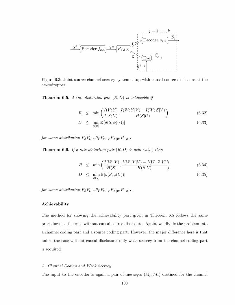
Encoder fk,n PY Z|X
Decoder gk,n
Eve
j = 1, . . . , k
Sk XnY n
Zn
Sj
Sj
Sj−1
Figure 6.3: Joint source-channel secrecy system setup with causal source disclosure at theeavesdropper
Theorem 6.5. A rate distortion pair (R,D) is achievable if
R ≤ min
(I(V ;Y )
I(S;U),I(W ;Y |V )− I(W ;Z|V )
H(S|U)
), (6.32)
D ≤ minφ(u)
E [d(S, φ(U))] (6.33)
for some distribution PSPU |SPV PW |V PX|WPY Z|X .
Theorem 6.6. If a rate distortion pair (R,D) is achievable, then
R ≤ min
(I(W ;Y )
H(S),I(W ;Y |V )− I(W ;Z|V )
H(S|U)
)(6.34)
D ≤ minφ(u)
E [d(S, φ(U))] (6.35)
for some distribution PSPU |SPV PW |V PX|WPY Z|X .
Achievability
The method for showing the achievability part given in Theorem 6.5 follows the same
procedures as the case without causal source disclosure. Again, we divide the problem into
a channel coding part and a source coding part. However, the major difference here is that
unlike the case without causal disclosure, only weak secrecy from the channel coding part
is required.
A. Channel Coding and Weak Secrecy
The input to the encoder is again a pair of messages (Mp,Ms) destined for the channel
103
decoder, with Mp representing a public message and Ms a secure message. The channel
decoder outputs the pair (Mp, Ms). We allow the channel encoder to use private random-
ization. We use the same definition given in Definition 6.2 for a channel code.
We make a further technical requirement (cf. [30]) for the channel input. That is,
conditioned on Mp, Ms is almost uniform. To be precise, we require
maxmp,ms,m′s
P[Ms = ms|Mp = mp]
P[Ms = m′s|Mp = mp]≤ 2nδn (6.36)
to hold for some δn →n 0. The source encoder we employ will produce message pairs
(Mp,Ms) that satisfy this condition, regardless of the source distribution.
Definition 6.8. The rate pair (Rs, Rp) is achievable under weak secrecy if for all (Ms,Mp)
satisfying (6.36), there exists a sequence of (Rs, Rp, n) channel codes such that
P[(Ms,Mp) 6= (Ms, Mp)
]→n 0 (6.37)
and
1
nI(Ms;Z
nMp)→n 0. (6.38)
Theorem 6.7. The pair (Rp, Rs) is achievable if
Rp ≤ I(V ;Y ) (6.39)
Rs ≤ I(W ;Y |V )− I(W ;Z|V ) (6.40)
for some PV PW |V PX|WPY Z|X .
The proof of Theorem 6.7 is provided in Appendix 6.5.5.
B. Source Coding
Under the same definition for a source code given in Definition 6.5, we make the following
modifications.
104
Definition 6.9. A rate distortion triple (R′s, R′p, D) is achievable under a given distortion
measure d(·, ·) if there exists a sequence of (R′s, R′p, k) source codes such that
P[Sk 6= gs(fs(S
k))]→k 0 (6.41)
and the message pair generated by the source encoder satisfies (6.36) for every n, and for
all PZn|MsMpsuch that 1
nI(Ms;Zn|Mp)→n 0
lim infk→∞
min{sj(zn,sj−1)}kj=1
E
1
k
k∑j=1
d(Sj , sj(Zn, Sj−1))
≥ D. (6.42)
Theorem 6.8. A rate distortion triple (R′s, R′p, D) is achievable if
R′p > I(S;U) (6.43)
R′s > H(S|U) (6.44)
D ≤ minφ(u)
E[d(S, φ(U))] (6.45)
for some PSPU |S.
The main idea in the proof of Theorem 6.8 is to use the public message to specify a
sequence Uk that is correlated with Sk, and use the secure message to encode the supplement
that is needed to fully specify the source sequence. The source encoder is defined in such a
way that, conditioned on the public message Mp, the adversary views the source as if it were
generated by passing Uk through a memoryless channel PS|U . With this perspective, the
past Sj−1 will no longer help the adversary; the eavesdropper’s best strategy is to choose a
function that maps Uj to Sj .
Below is a crucial lemma that shows how the weak secrecy provided by a good channel
code is used in analyzing the payoff. The result of this lemma is that we can view the
eavesdropper as having full knowledge of Mp and Sj−1 and no knowledge of Ms, which
fulfills our goal of creating a secure channel and a public channel. We show that, from the
eavesdropper’s perspective, knowledge of (Zn, Sj−1) is no more helpful than (Mp, Sj−1) in
easing the distortion.
105
Lemma 6.3. If PMpMs satisfies (6.36) for every n, and PZn|MpMssuch that 1
nI(Ms;Zn|Mp)→n
0, then for all ε > 0,
mins(j,sj−1,zn)
E
1
k
k∑j=1
d(Sj , s(j, S
j−1, Zn))
≥ mins(j,sj−1,mp)
E
1
k
k∑j=1
d(Sj , s(j, S
j−1,Mp))− δ(ε) (6.46)
for sufficiently large n, where δ(ε)→ 0 as ε→ 0.
The proof is provided in Appendix 6.5.6.
Now we have all the elements to prove Theorem 6.8. Again, we use the likelihood
encoder together with the analysis using the soft-covering lemmas.
Proof. We follow the convention of using P to denote the system induced distribution and
replace the single-letter distributions with P . Note that PS = PS .
Fix a distribution PSU = PSPU |S satisfying
minφ(u)
E[d(S, φ(U))] ≥ D (6.47)
and fix rates R′p, R′s such that
R′p > I(S;U), (6.48)
R′s > H(S|U) (6.49)
under PSU .
The distribution induced by the encoder and decoder is
PSkMpMsSk(sk,mp,ms, s
k) = PSk(sk)PLE(mp,ms|sk)PD(sk|mp,ms) (6.50)
where PLE(mp,ms|sk) is the source encoder; and PD(sk|mp,ms) is the decoder that recon-
structs the source sequence.
106
Codebook generation: We independently generate 2kR′p sequences in Uk according
to∏kj=1 PU (uj) and index them by mp ∈ [1 : 2kR
′p ]. We use C(k)
U to denote this random
codebook. For each mp ∈ [1 : 2kR′p ], we independently generate 2kR
′s sequences in Sk
according to∏kj=1 PS|U (sj |uj(mp)) and index them by (mp,ms) ∈ [1 : 2kR
′p ] × [1 : 2kR
′s ].
We use C(k)
S(mp) to denote this random codebook.
Encoder: The encoder PLE(mp,ms|sk) is the likelihood encoder that chooses (mp,ms)
stochastically according to the following probability:
PLE(m|sk) =L(m|sk)∑
m∈M L(m|sk)(6.51)
where m = (mp,ms), M = [1 : 2kR′p ]× [1 : 2kR
′s ], and
L(m|sk) = 1{sk = sk(m)} (6.52)
= PSk|Sk(sk|sk(m)). (6.53)
Decoder: The decoder is a codeword lookup decoder that simply reproduces
Sk(mp,ms).
Analysis: We first examine the error probability at the legitimate receiver by looking at
the system induced distribution P, and auxiliary distributions Q and Q′. Then we analyze
the distortion at the eavesdropper through another auxiliary distribution Q.
On the legitimate receiver side, let us define an idealized distribution Q that is of the
form in the soft-covering lemma, i.e. as if the codeword Sk is passed through a noise-free
memoryless channel. Formally, the idealized distribution Q is defined as
QSkMpMsUkSk(sk,mp,ms, u
k, sk)
= QMpMs(mp,ms)QUk|Mp(uk|mp)QSk|MpMs
(sk|mp,ms)QSk|Sk(sk|sk) (6.54)
=1
2k(R′p+R′s)1{uk = Uk(mp)}1{sk = Sk(mp,ms)}1{sk = sk} (6.55)
107
Note that the encoder PLE and decoder PD satisfy
PLE(mp,ms|sk) = QMpMS |Sk(mp,ms|sk) (6.56)
PD(sk|mp,ms) = QSk|MpMS(sk|mp,ms). (6.57)
Define another auxiliary distribution Q′ on a subset of the variables as
Q′MpUkSk(mp, u
k, sk) =1
2kR′p1{uk = Uk(mp)}
k∏j=1
PS|U (sj |Uj(mp)). (6.58)
Since Rs > I(S; S|U) = H(S|U) under P , applying the superposition soft-covering
Lemma 2.2, we have for some γ2 > 0
EC(k)
[∥∥∥QMpSk −Q′MpSk
∥∥∥TV
]≤ e−γ2k. (6.59)
Also since Rp > I(U ;S), applying the basic soft-covering lemma (Lemma 2.1), we have for
some γ1 > 0
EC(k)
[∥∥PSk −Q′Sk∥∥TV
]≤ e−γ1k. (6.60)
Using Property 2.1(c), (6.60) and (6.59), we obtain
EC(k) [‖PSk −QSk‖TV ] ≤ e−γ1k + e−γ2k , ε3k. (6.61)
By Property 2.1(e), (6.56) and (6.57), we have
EC(k)
[∥∥∥PSkMpMsSk−QSkMpMsSk
∥∥∥TV
]≤ ε3k. (6.62)
By construction of the idealized distribution Q,
PQ
[Sk 6= Sk
]= 0. (6.63)
108
Using Property 2.1(b), we obtain
PP
[Sk 6= Sk
]≤ ε3k. (6.64)
On the eavesdropper’s side, we denote the marginals of Q′ by Q(j) as follows:
Q(j)
MpUkSj(mp, u
k, sj) = Q′MpUkSj(mp, u
k, sj) (6.65)
where Q′ is defined in (6.58).
Therefore, by Property 2.1(c), (6.60) and (6.62), we obtain
EC(k)
[∥∥∥PMpSj − Q(j)
MpSj
∥∥∥TV
]≤ 2e−γ1k + e−γ2k. (6.66)
Note that under Q(j), we have the Markov relation
Sj − Uj(Mp)−MpSj−1. (6.67)
Also note that, since R′p > 0, invoking the soft-covering lemma gives us
EC(k)
[∥∥∥Q(j)Uj(Mp) − PU
∥∥∥TV
]≤ e−γ3k (6.68)
for some γ3 > 0.
Combining (6.64), (6.66) and (6.68) and the random coding argument, there exists a
codebook under which
PP[Sk 6= Sk
]≤ εk (6.69)
k∑j=1
∥∥∥PMpSj − Q(j)
MpSj
∥∥∥TV≤ εk (6.70)
k∑j=1
∥∥∥Quj(Mp) − PU∥∥∥TV≤ εk (6.71)
where εk = ε3k + k(2e−γ1k + e−γ2k) + ke−γ3k.
109

Finally, the distortion at the eavesdropper can be lower bounded by the following steps:
min{sj(zn,sj−1)}kj=1
E
1
k
k∑j=1
d(Sj , sj(Z
n, Sj−1))
≥ min{sj(mp,sj−1)}kj=1
E
1
k
k∑j=1
d(Sj , sj(Mp, S
j−1))− δk (6.72)
=1
k
k∑j=1
minsj(mp,sj−1)
EP[d(Sj , sj(Mp, S
j−1))]− δk (6.73)
≥ 1
k
k∑j=1
minsj(mp,sj−1)
EQ(j)
[d(Sj , sj(Mp, S
j−1))]− δk − εkdmax (6.74)
=1
k
k∑j=1
minφ(u)
EQ(j) [d (Sj , φ (uj(Mp)))]− δk − εkdmax (6.75)
≥ 1
k
k∑j=1
minφ(u)
EP [d (S, φ(U))]− δk − 2εkdmax (6.76)
where δk →k 0. Eq. (6.72) follows from Lemma 6.3; (6.74) follows from (6.70); (6.75)
follows from the Markov relation (6.67); and (6.76) follows from (6.71) and the fact that
Q(j)Sj |Uj (sj |uj) = PS|U (sj |uj). (6.77)
Now we return to proving Theorem 6.5 by rate matching from the channel coding
Theorem 6.7 and source coding Theorem 6.8, we can achieve
R ≤ min
(I(V ;Y )
I(S;U),I(W ;Y |V )− I(W ;Z|V )
H(S|U)
), (6.78)
D ≤ minφ(u)
E [d(S, φ(U))] (6.79)
for some distribution PSPU |SP V PW |V PX|WP Y Z|X .
An Improved Inner Bound
We can strengthen the above distortion analysis by taking into account the equivocation
of the public message. For source blocklength k, the equivocation of the public message
110
vanishes at a certain time k′ due to the eavesdropper’s ongoing accumulation of past source
symbols Sk′−1. Before time k′, the payoff is ∆, because the eavesdropper does not have
enough information to decode the public message. After time k′, the payoff is as given in
(6.79). The transition happens at
k′ =[I(V ;Y )− I(V ;Z)]+
I(S;U)Rk. (6.80)
This gives us an improved achievable region stated in the following theorem.
Theorem 6.9. A rate distortion pair (R,D) is achievable if
R ≤ min
(I(V ;Y )
I(S;U),I(W ;Y |V )− I(W ;Z|V )
H(S|U)
), (6.81)
D ≤ α
R·∆ +
(1− α
R
)·minφ(u)
E [d(S, φ(U))] (6.82)
for some distribution PSPU |SPV PW |V PX|WPY Z|X , where α = [I(V ;Y )−I(V ;Z)]+
I(S;U) .
Outer Bound
Now we give the proof for Theorem 6.6.
Proof. Introduce random variables Q1 ∼ Unif [1 : k], Q2 ∼ Unif [1 : n], independent of
(Sk, Xn, Y n, Zn). Define the random variables
U = (Zn, SQ1−1, Q1) (6.83)
V = (Y Q2−1, ZnQ2+1, Q2) (6.84)
W = (V, Sk) (6.85)
S = SQ1 (6.86)
(X,Y, Z) = (XQ2 , YQ2 , ZQ2). (6.87)
111

It can be verified that V −W −X − Y Z. First, we have
H(S|U)
= H(SQ1 |ZnSQ1−1Q1) (6.88)
=1
k
k∑j=1
H(Sj |ZnSj−1) (6.89)
=1
kH(Sk|Zn) (6.90)
=1
kH(Sk)− 1
kI(Sk;Zn) (6.91)
=1
kI(Sk;Y n)− 1
kI(Sk;Zn) +
1
kH(Sk|Y n) (6.92)
≤ 1
kI(Sk;Y n)− 1
kI(Sk;Zn) + εk (6.93)
=1
R
(1
nI(Sk;Y n)− 1
nI(Sk;Zn)
)+ εk (6.94)
=1
R
(1
n
n∑i=1
I(Sk;Yi|Y i−1Zni+1)− 1
n
n∑i=1
I(Sk;Zi|Y i−1Zni+1)
)+ εk (6.95)
=1
R(I(W ;Y |V )− I(W ;Z|V )) + εk (6.96)
where (6.93) follows from Fano’s inequality and εk →k 0. The step (6.95) uses the Csiszar
sum identity. Next, we have
H(S)
=1
R
1
n
(I(Sk;Y n) +H(Sk|Y n)
)(6.97)
≤ 1
R
1
n
n∑i=1
I(Sk;Y i|Y i−1) + εk (6.98)
≤ 1
R
1
n
n∑i=1
I(SkY i−1Zni+1;Y i) + εk (6.99)
=1
RI(SkY Q2−1ZnQ2+1;YQ2 ;YQ2 |Q2) + εk (6.100)
≤ 1
RI(W ;Y ) + εk. (6.101)
112
Finally,
D ≤ mins(j,sj−1,zn)
E
1
k
k∑j=1
d(Sj , s(j, S
j−1, Zn)) (6.102)
= mins(q1,sq1−1,zn)
E[d(SQ1 , s(Q1, S
Q1−1, Zn))]
(6.103)
= minφ(u)
E[d(S, φ(U))]. (6.104)
6.2.3 Binary Symmetric Broadcast Channel and Binary Source
To visualize Theorem 6.1 and Theorem 6.5, we will illustrate the results with a binary
symmetric broadcast channel (BSBCC) and binary source under Hamming distortion.
With the above setting, suppose Sj ∼ Bern(p), and the broadcast channel is binary
symmetric with crossover probabilities to the intended receiver and the eavesdropper p1
and p2, respectively. Assume p ≤ 0.5 and p1 < p2 < 0.5. This stochastically degraded
channel can be considered physically degraded in capacity calculations because none of the
mutual information quantities (or error probabilities) depend on the joint distribution. Let
us make the following definitions:
f(x) is the linear interpolation of the points(log n,
n− 1
n
), n = 1, 2, 3, ... (6.105)
d(x) , min(f(x), 1−maxsPS(s)), (6.106)
h(x) , x log1
x+ (1− x) log
1
1− xis the binary entropy function, (6.107)
x1 ∗ x2 , x1 ∗ (1− x2) + (1− x1) ∗ x2
is the binary convolution, (6.108)
where PS(·) is the probability mass function of the random variable S. The corresponding
rate-distortion regions for the cases without and with causal source disclosure are given in
the following corollaries.
113
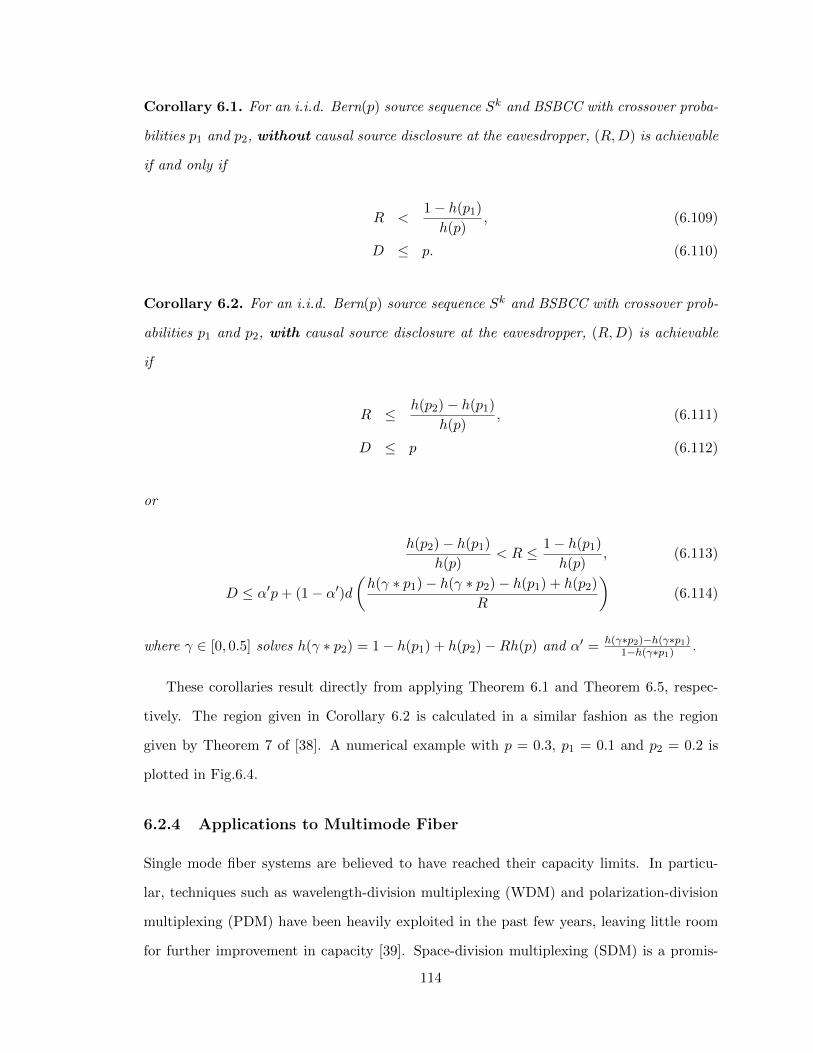
Corollary 6.1. For an i.i.d. Bern(p) source sequence Sk and BSBCC with crossover proba-
bilities p1 and p2, without causal source disclosure at the eavesdropper, (R,D) is achievable
if and only if
R <1− h(p1)
h(p), (6.109)
D ≤ p. (6.110)
Corollary 6.2. For an i.i.d. Bern(p) source sequence Sk and BSBCC with crossover prob-
abilities p1 and p2, with causal source disclosure at the eavesdropper, (R,D) is achievable
if
R ≤ h(p2)− h(p1)
h(p), (6.111)
D ≤ p (6.112)
or
h(p2)− h(p1)
h(p)< R ≤ 1− h(p1)
h(p), (6.113)
D ≤ α′p+ (1− α′)d(h(γ ∗ p1)− h(γ ∗ p2)− h(p1) + h(p2)
R
)(6.114)
where γ ∈ [0, 0.5] solves h(γ ∗ p2) = 1− h(p1) + h(p2)−Rh(p) and α′ = h(γ∗p2)−h(γ∗p1)1−h(γ∗p1) .
These corollaries result directly from applying Theorem 6.1 and Theorem 6.5, respec-
tively. The region given in Corollary 6.2 is calculated in a similar fashion as the region
given by Theorem 7 of [38]. A numerical example with p = 0.3, p1 = 0.1 and p2 = 0.2 is
plotted in Fig.6.4.
6.2.4 Applications to Multimode Fiber
Single mode fiber systems are believed to have reached their capacity limits. In particu-
lar, techniques such as wavelength-division multiplexing (WDM) and polarization-division
multiplexing (PDM) have been heavily exploited in the past few years, leaving little room
for further improvement in capacity [39]. Space-division multiplexing (SDM) is a promis-
114
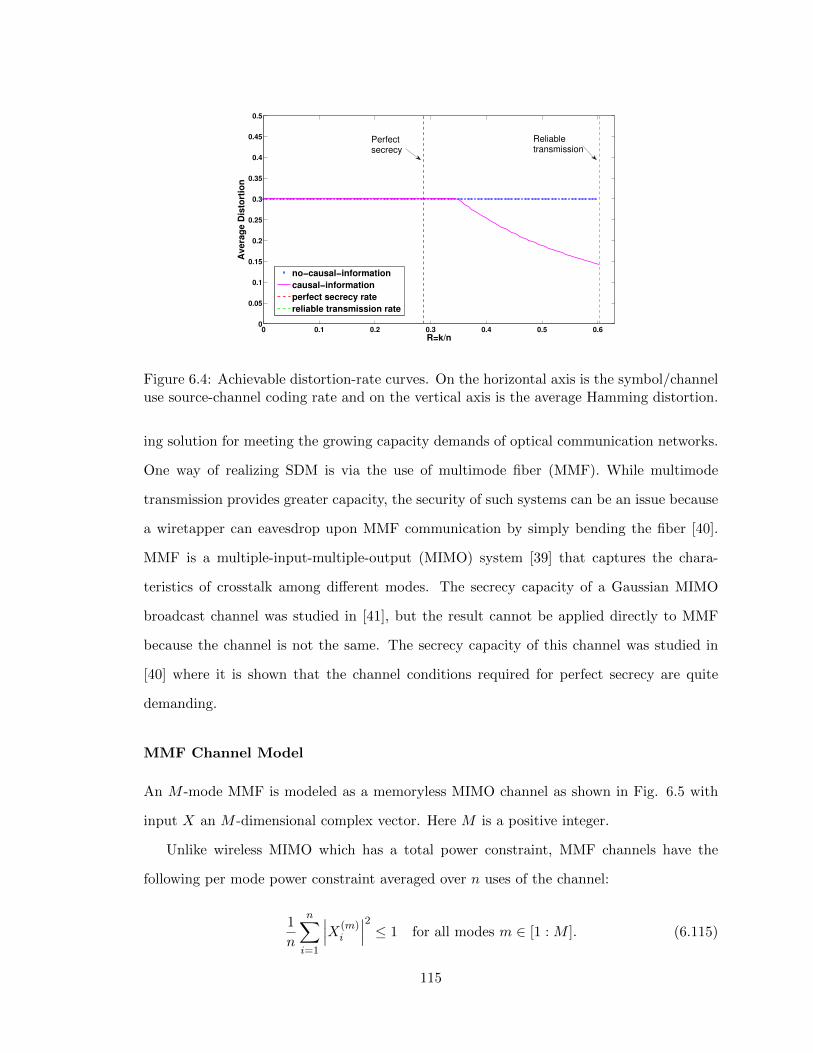
0 0.1 0.2 0.3 0.4 0.5 0.60
0.05
0.1
0.15
0.2
0.25
0.3
0.35
0.4
0.45
0.5
R=k/n
Avera
ge D
isto
rtio
n
no−causal−information
causal−information
perfect secrecy rate
reliable transmission rate
Perfectsecrecy
Reliabletransmission
Figure 6.4: Achievable distortion-rate curves. On the horizontal axis is the symbol/channeluse source-channel coding rate and on the vertical axis is the average Hamming distortion.
ing solution for meeting the growing capacity demands of optical communication networks.
One way of realizing SDM is via the use of multimode fiber (MMF). While multimode
transmission provides greater capacity, the security of such systems can be an issue because
a wiretapper can eavesdrop upon MMF communication by simply bending the fiber [40].
MMF is a multiple-input-multiple-output (MIMO) system [39] that captures the chara-
teristics of crosstalk among different modes. The secrecy capacity of a Gaussian MIMO
broadcast channel was studied in [41], but the result cannot be applied directly to MMF
because the channel is not the same. The secrecy capacity of this channel was studied in
[40] where it is shown that the channel conditions required for perfect secrecy are quite
demanding.
MMF Channel Model
An M -mode MMF is modeled as a memoryless MIMO channel as shown in Fig. 6.5 with
input X an M -dimensional complex vector. Here M is a positive integer.
Unlike wireless MIMO which has a total power constraint, MMF channels have the
following per mode power constraint averaged over n uses of the channel:
1
n
n∑i=1
∣∣∣X(m)i
∣∣∣2 ≤ 1 for all modes m ∈ [1 : M ]. (6.115)
115
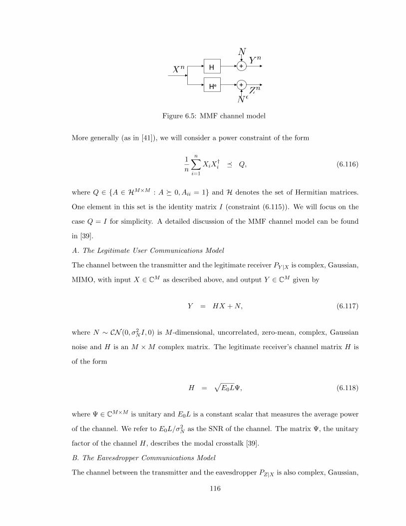
Figure 6.5: MMF channel model
More generally (as in [41]), we will consider a power constraint of the form
1
n
n∑i=1
XiX†i � Q, (6.116)
where Q ∈ {A ∈ HM×M : A � 0, Aii = 1} and H denotes the set of Hermitian matrices.
One element in this set is the identity matrix I (constraint (6.115)). We will focus on the
case Q = I for simplicity. A detailed discussion of the MMF channel model can be found
in [39].
A. The Legitimate User Communications Model
The channel between the transmitter and the legitimate receiver PY |X is complex, Gaussian,
MIMO, with input X ∈ CM as described above, and output Y ∈ CM given by
Y = HX +N, (6.117)
where N ∼ CN (0, σ2NI, 0) is M -dimensional, uncorrelated, zero-mean, complex, Gaussian
noise and H is an M ×M complex matrix. The legitimate receiver’s channel matrix H is
of the form
H =√E0LΨ, (6.118)
where Ψ ∈ CM×M is unitary and E0L is a constant scalar that measures the average power
of the channel. We refer to E0L/σ2N as the SNR of the channel. The matrix Ψ, the unitary
factor of the channel H, describes the modal crosstalk [39].
B. The Eavesdropper Communications Model
The channel between the transmitter and the eavesdropper PZ|X is also complex, Gaussian,
116

MIMO, with input X ∈ CM as described above, and output Z ∈ CM given by
Z = HeX +N e, (6.119)
where N e ∼ CN (0, σ2NeI, 0) is M -dimensional uncorrelated, zero-mean, complex, Gaussian
noise, and He is an M ×M complex matrix. The eavesdropper’s channel matrix He is of
the form
He =√E0Le
√ΦΨe, (6.120)
where Ψe ∈ CM×M is unitary, Φ is diagonal with positive entries, and E0Le is the average
power of the eavesdropper’s channel. Note that the eavesdropper has a different signal
to noise ratio SNRe = E0Le/σ2
Ne . The diagonal component Φ of the channel matrix He
corresponds to the mode-dependent loss (MDL) as introduced in [39].
Main Results
We now apply the results from Section 6.2.1 and 6.2.2 to the MMF model by finding the
rate distortion regions for the MMF model defined in (6.117) and (6.119) under the two
scenarios [42] [43]. In this section, as before, we assume the channels are time-invariant.
First of all, we will give the achievable rate region under strong secrecy (therefore also under
weak secrecy).
Theorem 6.10. The following rate region for one confidential and one non-confidential
message is achievable under strong secrecy for a complex Gaussian channel:
Rs ≤ log|HKH† + σ2
NI||σ2NI|
− log|HeKHe† + σ2
NeI||σ2NeI|
(6.121)
Rp ≤ log|HQH† + σ2
NI||HKH† + σ2
NI|(6.122)
for some K and Q, where 0 � K � Q, K ∈ HM×M , Q satisfies the power constraint in
(6.116), and H and He are the channel gain matrices.
117
Proof. According to Theorem 6.2 and 6.3,
Rs ≤ I(W ;Y |V )− I(W ;Z|V ) (6.123)
Rp ≤ I(V ;Y ) (6.124)
for some V −W −X − Y Z and E[XX†] � Q, is an achievable rate pair.
We restrict the channel input X to be a circularly symmetric complex Gaussian vector.
Let V ∼ CN (0, Q −K, 0) and B ∼ CN (0,K, 0) such that B and V are independent, and
W = X = V + B. Therefore, X ∼ CN (0, Q, 0) satisfies the power constraint. Similar
to results in [41], the rate pair (Rs, Rp) satisfying inequalities (6.121) and (6.122) can be
achieved.
An immediate corollary follows directly from the above theorem.
Corollary 6.3. The following rate pairs are achievable under strong secrecy for MMF with
channel gains defined in (6.118) and (6.120) and equal full power allocation Q = I:
Rs ≤ log|SNRK + I|
|SNReΨeKΨe†Φ + I|(6.125)
Rp ≤ log|(SNR + 1)I||SNRK + I|
(6.126)
for some K where 0 � K � I, K ∈ HM×M , SNR = E0L/σ2N and SNRe = E0L
e/σ2Ne.
With the secrecy capacity region of MMF, we can evaluate its rate distortion region
(R,D) under the two extreme cases, without and with causal source disclosure at the
eavesdropper’s decoder respectively. For the case without causal source disclosure, we give
a sufficient condition to force maximum average distortion ∆ between the transmitter and
the eavesdropper. For the case with causal source disclosure, we give an achievable rate-
distortion region and look at the particular case of Hamming distortion.
Theorem 6.11. For an i.i.d source sequence Sk, if
minj∈{1,...,M}
φj <SNR
SNRe (6.127)
118
where φj’s are the diagonal entries of Φ, then the following rate distortion pair (R,D) is
achievable without causal source disclosure at the eavesdropper:
R <M log(SNR + 1)
H(S)(6.128)
D ≤ ∆. (6.129)
Theorem 6.11 follows from Theorem 6.1 and Corollary 6.3. Note that (6.127) is a
sufficient condition for the existence of a secure channel with strictly positive rate from
the transmitter to the legitimate receiver. A discussion of this condition is provided in
Appendix 6.5.7.
Theorem 6.12. For an i.i.d. source sequence Sk and Hamming distortion, the following
distortion rate curve D(R) is in the achievable region with causal source disclosure at the
eavesdropper:
D = d(H(S)), if R ≤ R∗sH(S)
(6.130)
D = α(K)∆ + (1− α(K)) d
(Rs(K)
R
),
ifR∗sH(S)
< R ≤R∗pH(S)
(6.131)
where d(·) is as defined in (6.106); K , {K ∈ HM×M , 0 � K � I},
R∗s = maxK′∈K
log|SNRK ′ + I|
|SNRe√
ΦΨeK ′Ψe†√
Φ + I|, (6.132)
R∗p = M log(SNR + 1), (6.133)
Rs(K) = log|SNRK + I|
|SNRe√
ΦΨeKΨe†√
Φ + I|, (6.134)
α(K) =β(K)− γ(K)
β(K), (6.135)
β(K) = log|(SNR + 1)I||SNRK + I|
, (6.136)
γ(K) = log|SNReΦ + I|
|SNRe√
ΦΨeKΨe†√
Φ + I|. (6.137)
119
The result given in Theorem 6.12 can be derived directly from Theorem 6.5 and Corollary
6.3.
Numerical Results
In this section, we present numerical results illustrating achievable rate distortion regions
of an MMF under the two information models with a time-invariant channel. Let us con-
sider measuring the eavesdropper’s distortion using Hamming distortion and a Bern(p)
i.i.d. source sequence. Fig. 3 shows numerical results corresponding to Theorem 6.11 and
Theorem 6.12 under equal power allocation. The channels are simulated as a 4−mode MMF
with SNR = 20dB, SNRe = 10dB, and MDL = 20dB.
In each plot, the vertical line on the right is the maximum reliable transmission rate be-
tween the transmitter and the legitimate receiver and the vertical line on the left is the max-
imum perfect secrecy transmission rate that can be obtained with separate source-channel
coding. The horizontal line is the maximum distortion which is also the rate distortion
curve from Theorem 6.11 with no causal source disclosure at the eavesdropper. The curve
obtained from Theorem 6.12 shows the tradeoff between the transmission rate between the
transmitter and the legitimate receiver and the distortion forced on the eavesdropper with
causal source disclosure. We see in Fig. 6.6(a), p = 0.3, that with our source-channel coding
analysis, we gain a free region for maximum distortion, as if under perfect secrecy, (from
the left vertical line to the kink) because we effectively use the redundancy of the source.
In Fig. 6.6(b) with p = 0.5, since there is no redundancy in the source, the distortion curve
drops immediately after the maximum perfect secrecy rate. Note that the transmission
rates are not considered beyond the right vertical lines because they are above the maxi-
mum reliable transmission rates and the legitimate receiver cannot losslesly reconstruct the
source sequences.
120
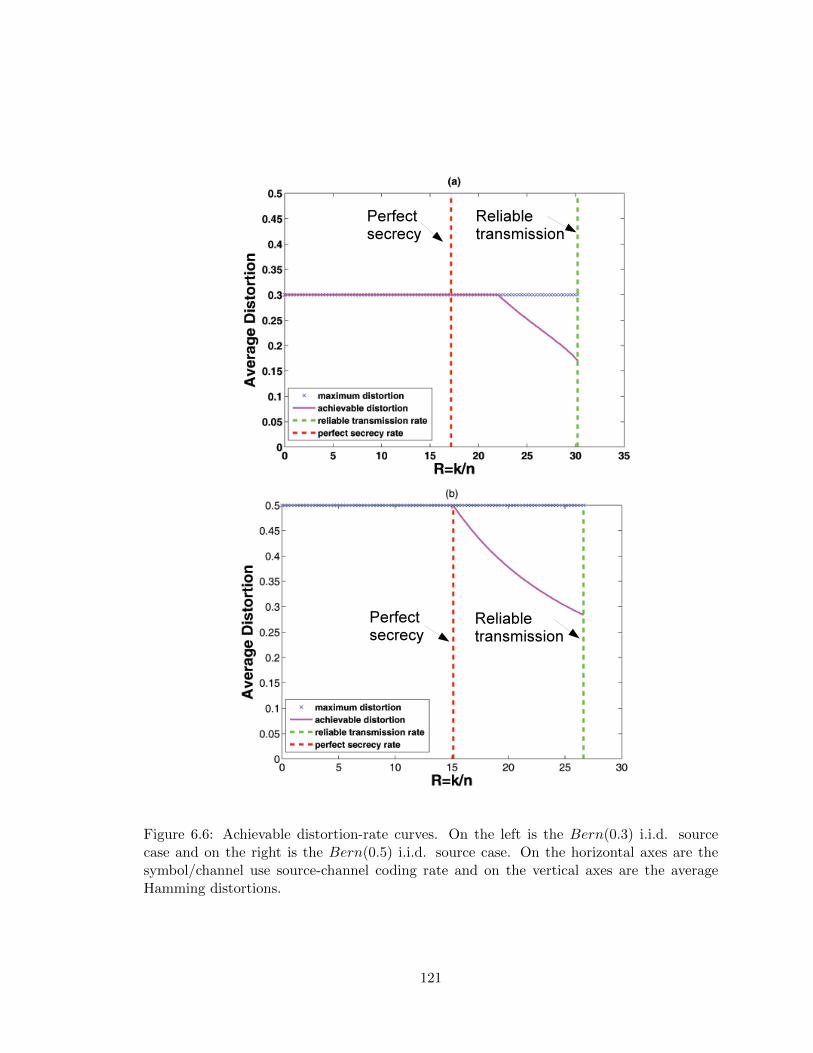
Figure 6.6: Achievable distortion-rate curves. On the left is the Bern(0.3) i.i.d. sourcecase and on the right is the Bern(0.5) i.i.d. source case. On the horizontal axes are thesymbol/channel use source-channel coding rate and on the vertical axes are the averageHamming distortions.
121
6.3 Joint Source-Channel Security
We re-approach the setting considered in Section 6.2.2. Instead of operationally separating
the encodings from source compression and channel coding, we use a joint source-channel
coding technique – hybrid coding to achieve better secrecy performance. The analysis relies
on the likelihood encoder.
6.3.1 Problem Revisit
Although this is a revisit of the problem we have introduced in Section 6.2.2, we make a
simplification here by only considering the same blocklength for the source sequence and
channel input sequence. Also, we expand the problem to allow lossy reconstruction of the
source at the legitimate receiver. For clarity, the problem formulation is restated as follows.
We want to determine conditions for a joint source-channel secrecy system that guar-
antee reliable communication to the legitimate receiver while a certain level of distortion
can be forced to the eavesdropper. The input of the system is an i.i.d. source sequence
Sn distributed according to∏nt=1 PS(st) and the channel is a memoryless broadcast chan-
nel∏nt=1 PY Z|X(yt, zt|xt). The source realization is causally disclosed to the eavesdropper
during decoding. The source-channel coding model satisfies the following constraints:
• Encoder fn : Sn 7→ X n (possibly stochastic);
• Legitimate receiver decoder gn : Yn 7→ Sn (possibly stochastic);
• Eavesdropper decoders {PSt|ZnSt−1}nt=1.
The system performance is measured by a distortion metric d(·, ·) as follows:
• Average distortion for the legitimate receiver:
lim supn→∞
E[d(Sn, Sn)
]≤ Db
• Minimum average distortion for the eavesdropper:
lim infn→∞
min{PSt|ZnSt−1}nt=1
E[d(Sn, Sn)] ≥ De.
122
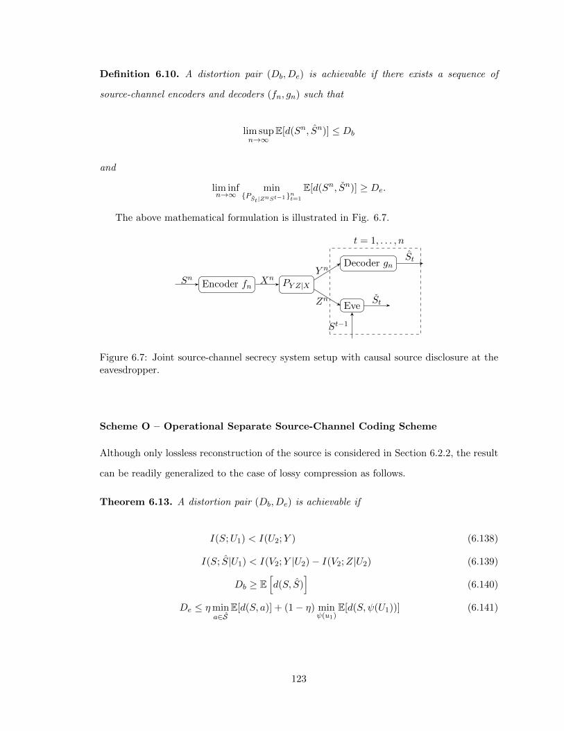
Definition 6.10. A distortion pair (Db, De) is achievable if there exists a sequence of
source-channel encoders and decoders (fn, gn) such that
lim supn→∞
E[d(Sn, Sn)] ≤ Db
and
lim infn→∞
min{PSt|ZnSt−1}nt=1
E[d(Sn, Sn)] ≥ De.
The above mathematical formulation is illustrated in Fig. 6.7.
Encoder fn PY Z|X
Decoder gn
Eve
t = 1, . . . , n
Sn XnY n
Zn
St
St
St−1
Figure 6.7: Joint source-channel secrecy system setup with causal source disclosure at theeavesdropper.
Scheme O – Operational Separate Source-Channel Coding Scheme
Although only lossless reconstruction of the source is considered in Section 6.2.2, the result
can be readily generalized to the case of lossy compression as follows.
Theorem 6.13. A distortion pair (Db, De) is achievable if
I(S;U1) < I(U2;Y ) (6.138)
I(S; S|U1) < I(V2;Y |U2)− I(V2;Z|U2) (6.139)
Db ≥ E[d(S, S)
](6.140)
De ≤ ηmina∈S
E[d(S, a)] + (1− η) minψ(u1)
E[d(S, ψ(U1))] (6.141)
123

for some distribution PSPS|SPU1|SPU2PV2|U2PX|V2
PY Z|X , where
η =[I(U2;Y )− I(U2;Z)]+
I(S;U1). (6.142)
Since the source coding and channel coding parts of the above scheme are almost inde-
pendent (with some technical details), we refer to it as operationally separate source-channel
coding – Scheme O.
6.3.2 Secure Hybrid Coding
Hybrid coding is a joint source-channel coding technique [8] where 1) the encoder generates
a digital codeword from the analog source and selects the channel input as a symbol-by-
symbol function of the codeword and the source; and 2) the decoder recovers the digital
codeword from the analog channel output and selects the source estimate as a symbol-by-
symbol function of the codeword and the channel output. It has been shown that this joint
source-channel code is optimal at least for point-to-point communication. For the purpose
of achieving secrecy, the symbol-by-symbol mapping (deterministic) to the channel input in
the encoding stage is modified to be stochastic.
Scheme I – Basic Hybrid Coding
An achievability region using basic secure hybrid coding is given in the following theorem.
Theorem 6.14. A distortion pair (Db, De) is achievable if
I(U ;S) < I(U ;Y ) (6.143)
Db ≥ E[d(S, φ(U, Y ))] (6.144)
De ≤ β minψ0(z)
E[d(S, ψ0(Z))] + (1− β) minψ1(u,z)
E[d(S, ψ1(U,Z))] (6.145)
where
β = min
{[I(U ;Y )− I(U ;Z)]+
I(S;U |Z), 1
}(6.146)
124
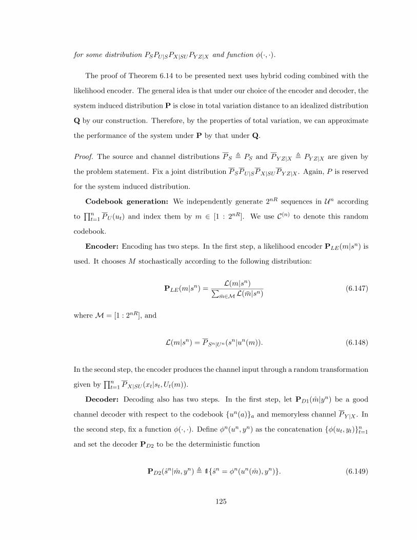
for some distribution PSPU |SPX|SUPY Z|X and function φ(·, ·).
The proof of Theorem 6.14 to be presented next uses hybrid coding combined with the
likelihood encoder. The general idea is that under our choice of the encoder and decoder, the
system induced distribution P is close in total variation distance to an idealized distribution
Q by our construction. Therefore, by the properties of total variation, we can approximate
the performance of the system under P by that under Q.
Proof. The source and channel distributions PS , PS and P Y Z|X , PY Z|X are given by
the problem statement. Fix a joint distribution PSPU |SPX|SUP Y Z|X . Again, P is reserved
for the system induced distribution.
Codebook generation: We independently generate 2nR sequences in Un according
to∏nt=1 PU (ut) and index them by m ∈ [1 : 2nR]. We use C(n) to denote this random
codebook.
Encoder: Encoding has two steps. In the first step, a likelihood encoder PLE(m|sn) is
used. It chooses M stochastically according to the following distribution:
PLE(m|sn) =L(m|sn)∑
m∈M L(m|sn)(6.147)
where M = [1 : 2nR], and
L(m|sn) = PSn|Un(sn|un(m)). (6.148)
In the second step, the encoder produces the channel input through a random transformation
given by∏nt=1 PX|SU (xt|st, Ut(m)).
Decoder: Decoding also has two steps. In the first step, let PD1(m|yn) be a good
channel decoder with respect to the codebook {un(a)}a and memoryless channel P Y |X . In
the second step, fix a function φ(·, ·). Define φn(un, yn) as the concatenation {φ(ut, yt)}nt=1
and set the decoder PD2 to be the deterministic function
PD2(sn|m, yn) , 1{sn = φn(un(m), yn)}. (6.149)
125
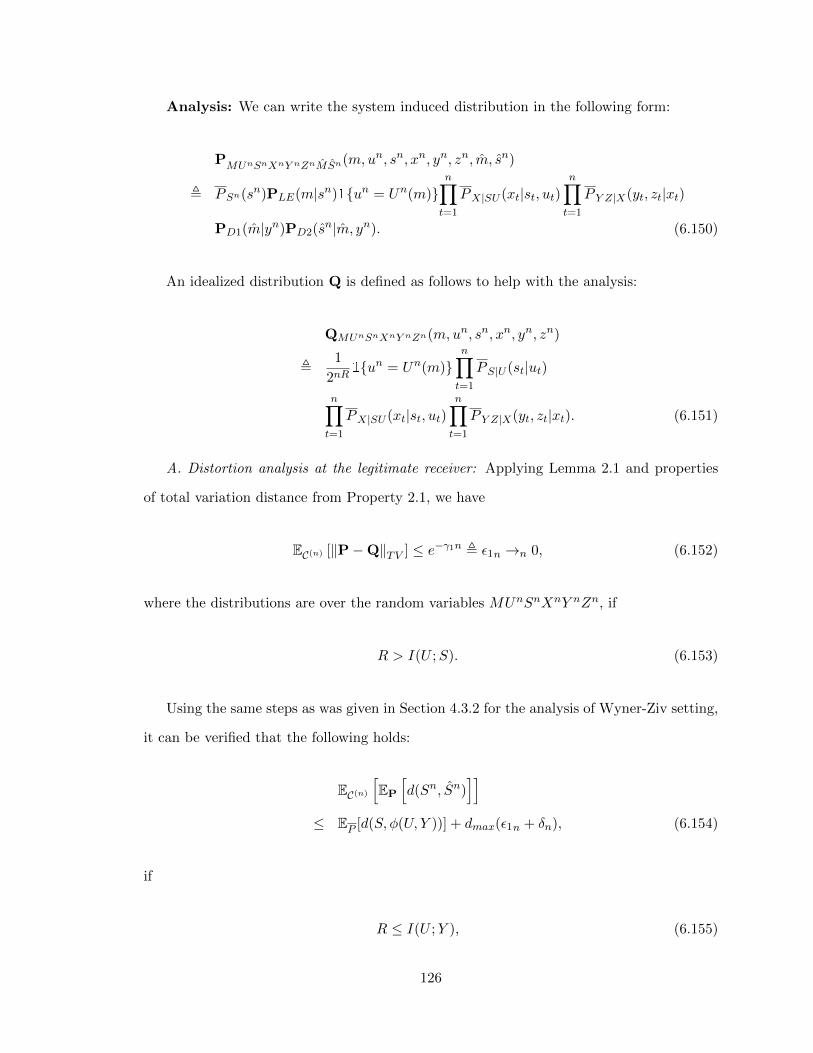
Analysis: We can write the system induced distribution in the following form:
PMUnSnXnY nZnMSn(m,un, sn, xn, yn, zn, m, sn)
, PSn(sn)PLE(m|sn)1{un = Un(m)}n∏t=1
PX|SU (xt|st, ut)n∏t=1
P Y Z|X(yt, zt|xt)
PD1(m|yn)PD2(sn|m, yn). (6.150)
An idealized distribution Q is defined as follows to help with the analysis:
QMUnSnXnY nZn(m,un, sn, xn, yn, zn)
,1
2nR1{un = Un(m)}
n∏t=1
PS|U (st|ut)
n∏t=1
PX|SU (xt|st, ut)n∏t=1
P Y Z|X(yt, zt|xt). (6.151)
A. Distortion analysis at the legitimate receiver: Applying Lemma 2.1 and properties
of total variation distance from Property 2.1, we have
EC(n) [‖P−Q‖TV ] ≤ e−γ1n , ε1n →n 0, (6.152)
where the distributions are over the random variables MUnSnXnY nZn, if
R > I(U ;S). (6.153)
Using the same steps as was given in Section 4.3.2 for the analysis of Wyner-Ziv setting,
it can be verified that the following holds:
EC(n)
[EP
[d(Sn, Sn)
]]≤ EP [d(S, φ(U, Y ))] + dmax(ε1n + δn), (6.154)
if
R ≤ I(U ;Y ), (6.155)
126

where δn →n 0.
B. Distortion analysis at the eavesdropper: On the eavesdropper side, we make the
following observation. Define an auxiliary distribution
Q(i)
SiZn(si, zn) ,
n∏t=1
PZ(zt)i∏
j=1
PS|Z(sj |zj) (6.156)
and under Q(i),
Si − Zi − ZnSi−1. (6.157)
Recall that
QMZnSi(m, zn, si)
=1
2nR
n∏t=1
PZ|U (zt|Ut(m))i∏
j=1
PS|ZU (sj |zj , Uj(m)) (6.158)
and under Q, the following Markov relation holds:
Si − ZiUi(M)− ZnSi−1M. (6.159)
Apply Lemma 2.2 with the following symbol assignment:
(U, V,X,Z)← (∅, U, Z, S) (6.160)
where on the left are the variables from Lemma 2.2 and on the right are the variables from
our analysis. We obtain
EC(n)
[∥∥∥Q(i)
ZnSi−QZnSi
∥∥∥TV
]≤ e−γ2n (6.161)
for any β < R−I(U ;Z)I(S;U |Z) , i ≤ βn, where γ2 > 0 depends on the gap R−I(U ;Z)
I(S;U |Z) −β. Consequently,
EC(n)
[∥∥∥Q(i)
ZnSi−PZnSi
∥∥∥TV
]≤ e−γ1n + e−γ2n. (6.162)
127
Also note that since R > 0, we have
EC(n)
[∥∥Qui(M) − PU∥∥TV
]≤ e−γ3n. (6.163)
Therefore, combining (6.152), (6.338), (6.340), and (6.154), there exists a codebook C(n)
such that
n∑i=1
‖PMZnSi −QMZnSi‖TV ≤ εn (6.164)
n∑i=1
∥∥∥PZnSi − Q(i)
ZnSi
∥∥∥TV≤ εn (6.165)
n∑i=1
∥∥Qui(M) − PU∥∥TV≤ εn (6.166)
EP[d(Sn, Sn)
]≤ EP
[d(Sn, Sn)
]+ εn (6.167)
where εn = n (2e−nγ1 + e−nγ2 + e−nγ3) + dmax(ε1n + δn)→n 0.
Now we can bound the distortion at the eavesdropper by breaking it down into two
sections. The distortion after the time transition βn can be lower bounded by the following:
min{ψ1i(s
i−1,zn)}EP
1
k
n∑i=j
d(Si, ψ1i(Si−1, Zn))
=
1
k
n∑i=j
minψ1i(s
i−1,zn)EP[d(Si, ψ1i(S
i−1, Zn))]
(6.168)
≥ 1
k
n∑i=1
minψ1i(s
i−1,zn,m)EP[d(Si, ψ1i(S
i−1, Zn,M))]
(6.169)
≥ 1
k
n∑i=j
minψ1i(s
i−1,zn,m)EQ[d(Si, ψ1i(S
i−1, Zn,M))]− εndmax (6.170)
=1
k
n∑i=j
minψ1(u,z)
EQ [d(Si, ψ1(ui(M), Zi))]− εndmax (6.171)
≥ 1
k
n∑i=j
minψ1(u,z)
EP [d(S, ψ1(U,Z))]− 2εndmax (6.172)
128
j = βn+ 1 (6.173)
k = (1− β)n (6.174)
where (6.170) is from (6.164), (6.171) uses the Markov relation given in (6.159), and (6.172)
uses (6.166) and the fact that
QZiSi|Ui(zi, si|ui) = PZ|U (zi|ui)PS|ZU (si|zi, ui). (6.175)
Similarly, we can bound the distortion before the time transition βn by the following
steps:
min{ψ0i(s
i−1,zn)}iEP
[1
k
k∑i=1
d(Si, ψ0i(Si−1, Zn))
]
=1
k
k∑i=1
minψ0i(s
i−1,zn)EP[d(Si, ψ0i(S
i−1, Zn))]
(6.176)
≥ 1
k
k∑i=1
minψ0i(s
i−1,zn)EQ(i)
[d(Si, ψ0i(S
i−1, Zn))]− εndmax (6.177)
=1
k
k∑i=1
minψ0(z)
EQ(i) [d(Si, ψ0(Zi))]− εndmax (6.178)
=1
k
k∑i=1
minψ0(z)
EP [d(S, ψ0(Z))]− εndmax (6.179)
k = βn (6.180)
where (6.177) is from (6.165), (6.178) uses the Markov relation given in (6.325), and (6.179)
uses the definition of Q given in (6.156).
Collecting (6.153), (6.155) and (6.167), and taking the average of the distortion at the
eavesdropper over the entire blocklength n from (6.172) and (6.179) finishes the proof.
Scheme II – Superposition Hybrid Coding
An achievability region using superposition secure hybrid coding is given in the following
theorem.
129

Theorem 6.15. A distortion pair (Db, De) is achievable if
I(V ;S) < I(UV ;Y ) (6.181)
Db ≥ E [d(S, φ(V, Y ))] (6.182)
De ≤ min{β, α} minψ0(z)
E [d(S, ψ0(Z))]
+ (α−min{β, α}) minψ1(u,z)
E [d(S, ψ1(U,Z))]
+(1− α) minψ2(v,z)
E [d(S, ψ2(V,Z))] (6.183)
where
β = min
{[I(U ;Y )− I(U ;Z)]+
I(S;U |Z), 1
}(6.184)
α = min
{[rs − I(Z;V |U)]+
I(S;V |ZU), 1
}(6.185)
rs = min{I(V ;Y |U), I(UV ;Y )− I(S;U)} (6.186)
for some distribution PSPV |SPU |V PX|SUV PY Z|X and function φ(·, ·).
The proof of Theorem 6.15 follows the same lines as the proof of Theorem 6.14 with
the modification of using a superposition codebook and the superposition version of the
soft-covering lemma. The proof is provided in Appendix 6.5.8.
Under Scheme II, the distortion at the eavesdropper can potentially experience two
transitions at βn and αn due to the superposition structure of the code.
6.3.3 Scheme Comparision
The relations of Scheme O, I and II can be summarized in the following corollaries.
Corollary 6.4. Scheme II generalizes Scheme I.
To see this, notice that we can let U = ∅ in Theorem 6.15. In fact, Scheme II simplifies
to Scheme I if β ≥ α.
Corollary 6.5. Scheme O is a special case of Scheme II.
130
Proof. Identify the following assignment of random variables from Theorem 6.13 to 6.15
U ← U1U2 (6.187)
V ← SV2. (6.188)
Substituting this assignment to the inequalities in Theorem 6.15 for the case α > β, we
get
I(S; S) < I(V2;Y ). (6.189)
It is easy to verify that the conditions given in Theorem 6.13 satisfy (6.189).
Substituting the assignment to (6.184) and (6.185) gives us
β =[I(U2;Y )− I(U2;Z)]+
I(S;U1)= η (6.190)
α = 1. (6.191)
Moreover, by the statistical independence of SU1 and U2V2Z
minψ0(z)
E[d(S, ψ0(Z))] = mina
E[d(S, a)] (6.192)
minψ1(u,z)
E[d(S, ψ1(U,Z))] = minψ1(u1,u2,z)
E[d(S, ψ1(U1, U2, Z))] (6.193)
= minψ(u1)
E[d(S, ψ(U1))]. (6.194)
6.3.4 The Perfect Secrecy Outer Bound
Theorem 6.16. If (Db, De) is achievable, then
I(S;U) ≤ I(U ;Y ) (6.195)
Db ≥ E[d(S, φ(U, Y ))] (6.196)
De ≤ mina∈S
E[d(S, a)] (6.197)
131
for some distribution PSPU |SPX|SUPY Z|X and function φ(·, ·).
This trivial outer bound can be verified by using the optimality of hybrid coding for
point-to-point communication and the fact that the estimation by the eavesdropper cannot
be worse than the a-priori estimation of the source. Note that (6.195) and (6.196) are
no different from the requirement for point-to-point source-channel coding. But we state
it this way to emphasize that hybrid coding does achieve optimality for point-to-point
communication.
6.3.5 Numerical Example
The source is distributed i.i.d. according to Bern(p) and the channels are binary symmetric
channels with crossover probabilities p1 = 0 and p2 = 0.3. For simplicity, we require lossless
decoding at the legitimate receiver. Hamming distance is considered for distortion at the
eavesdropper.
A numerical comparison of Scheme I with Scheme O is demonstrated in Fig. 6.8. The
choice of auxiliary random variable U in Scheme I is SX, which may not necessarily be the
optimum choice but is good enough to outperform Scheme O. Scheme II is not numerically
evaluated. However, because of Corollary 6.4 and 6.5, we know analytically that Scheme II
is no worse than O or I.
6.4 Summary
In this chapter, secure source-channel coding models have been studied. We have considered
two main ideas: operationally separate source-channel coding and hybrid coding. Follow-
ing the trace of developing secure source coding, we have investigated compression over a
noisy wiretap channel under the naive formulation without causal source disclosure and the
stronger formulation with causal source disclosure at the decoder. The theoretical results
have been applied to an multimode fiber channel.
We have shown that, under the naive formulation, with a general broadcast channel and
any distortion measure, it is possible with an operationally separate source-channel coding
scheme to send the source at the maximum rate that guarantees lossless reconstruction at
132
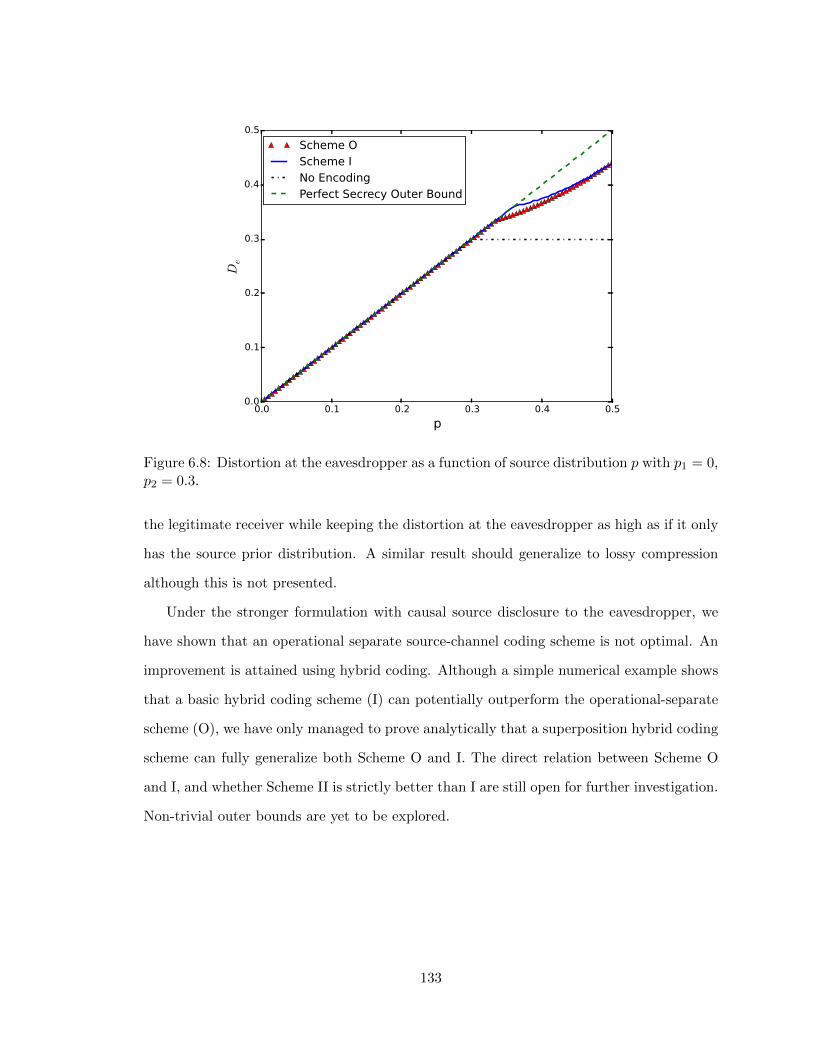
0.0 0.1 0.2 0.3 0.4 0.5
p
0.0
0.1
0.2
0.3
0.4
0.5
De
Scheme OScheme INo EncodingPerfect Secrecy Outer Bound
Figure 6.8: Distortion at the eavesdropper as a function of source distribution p with p1 = 0,p2 = 0.3.
the legitimate receiver while keeping the distortion at the eavesdropper as high as if it only
has the source prior distribution. A similar result should generalize to lossy compression
although this is not presented.
Under the stronger formulation with causal source disclosure to the eavesdropper, we
have shown that an operational separate source-channel coding scheme is not optimal. An
improvement is attained using hybrid coding. Although a simple numerical example shows
that a basic hybrid coding scheme (I) can potentially outperform the operational-separate
scheme (O), we have only managed to prove analytically that a superposition hybrid coding
scheme can fully generalize both Scheme O and I. The direct relation between Scheme O
and I, and whether Scheme II is strictly better than I are still open for further investigation.
Non-trivial outer bounds are yet to be explored.
133
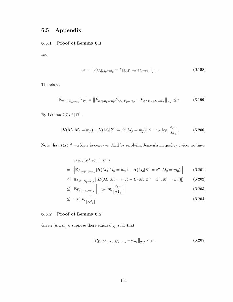
6.5 Appendix
6.5.1 Proof of Lemma 6.1
Let
εzn =∥∥PMs|Mp=mp − PMs|Zn=znMp=mp
∥∥TV
. (6.198)
Therefore,
EPZn|Mp=mp[εzn ] =
∥∥PZn|Mp=mpPMs|Mp=mp − PZnMs|Mp=mp
∥∥TV≤ ε. (6.199)
By Lemma 2.7 of [17],
|H(Ms|Mp = mp)−H(Ms|Zn = zn,Mp = mp)| ≤ −εzn logεzn
|Ms|. (6.200)
Note that f(x) , −x log x is concave. And by applying Jensen’s inequality twice, we have
I(Ms;Zn|Mp = mp)
=∣∣∣EPZn|Mp=mp
[H(Ms|Mp = mp)−H(Ms|Zn = zn,Mp = mp)]∣∣∣ (6.201)
≤ EPZn|Mp=mp[|H(Ms|Mp = mp)−H(Ms|Zn = zn,Mp = mp)|] (6.202)
≤ EPZn|Mp=mp
[−εzn log
εzn
|Ms|
](6.203)
≤ −ε logε
|Ms|. (6.204)
6.5.2 Proof of Lemma 6.2
Given (ms,mp), suppose there exists θmp such that
∥∥PZn|Mp=mpMs=ms − θmp∥∥TV≤ εn (6.205)
134
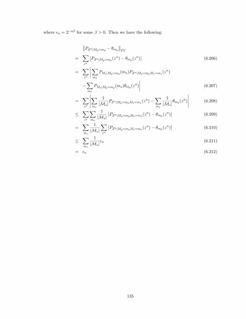
where εn = 2−nβ for some β > 0. Then we have the following:
∥∥PZn|Mp=mp − θmp∥∥TV
=∑zn
∣∣PZn|Mp=mp(zn)− θmp(zn)
∣∣ (6.206)
=∑zn
∣∣∣∣∑ms
PMs|Mp=mp(ms)PZn|Mp=mpMs=ms(zn)
−∑ms
PMs|Mp=mp(ms)θmp(zn)
∣∣∣∣ (6.207)
=∑zn
∣∣∣∣∣∑ms
1
|Ms|PZn|Mp=mpMs=ms(z
n)−∑ms
1
|Ms|θmp(z
n)
∣∣∣∣∣ (6.208)
≤∑zn
∑ms
1
|Ms|∣∣PZn|Mp=mpMs=ms(z
n)− θmp(zn)∣∣ (6.209)
=∑ms
1
|Ms|∑zn
∣∣PZn|Mp=mpMs=ms(zn)− θmp(zn)
∣∣ (6.210)
≤∑ms
1
|Ms|εn (6.211)
= εn (6.212)
135
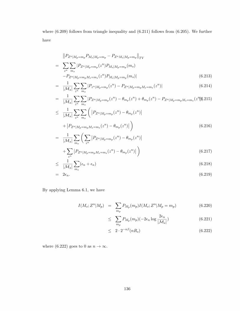
where (6.209) follows from triangle inequality and (6.211) follows from (6.205). We further
have
∥∥PZn|Mp=mpPMs|Mp=mp − PZnMs|Mp=mp
∥∥TV
=∑zn
∑ms
|PZn|Mp=mp(zn)PMs|Mp=mp(ms)
−PZn|Mp=mpMs=ms(zn)PMs|Mp=mp(ms)| (6.213)
=1
|Ms|∑zn
∑ms
|Pzn|Mp=mp(zn)− PZn|Mp=mpMs=ms(z
n)| (6.214)
=1
|Ms|∑zn
∑ms
|PZn|Mp=mp(zn)− θmp(zn) + θmp(z
n)− PZn|Mp=mpMs=ms(zn)|(6.215)
≤ 1
|Ms|∑zn
∑ms
( ∣∣PZn|Mp=mp(zn)− θmp(zn)
∣∣+∣∣PZn|Mp=mpMs=ms(z
n)− θmp(zn)∣∣ ) (6.216)
=1
|Ms|∑ms
(∑zn
∣∣PZn|Mp=mp(zn)− θmp(zn)
∣∣+∑zn
∣∣PZn|Mp=mpMs=ms(zn)− θmp(zn)
∣∣ ) (6.217)
≤ 1
|Ms|∑ms
(εn + εn) (6.218)
= 2εn. (6.219)
By applying Lemma 6.1, we have
I(Ms;Zn|Mp) =
∑mp
PMp(mp)I(Ms;Zn|Mp = mp) (6.220)
≤∑mp
PMp(mp)(−2εn log2εn|Ms|
) (6.221)
≤ 2 · 2−nβ(nRs) (6.222)
where (6.222) goes to 0 as n→∞.
136
6.5.3 Proof of (6.24)
For each i, we have
I(Si;Zn|Mp) ≤ I(MsSi;Z
n|Mp) (6.223)
= I(Ms;Zn|Mp) + I(Si;Z
n|MsMp) (6.224)
≤ ε (6.225)
for large enough n. Eq. (6.225) follows from strong secrecy of the channel and Fano’s
inequality. Note that weak secrecy is not sufficient to give us the desired result in our proof.
We now define
Pi , PSiZnMp (6.226)
Pi , PMpPSi|MpPZn|Mp
(6.227)
i.e. Pi is the Markov chain Si −Mp − Zn. By Pinsker’s inequality,
||Pi − Pi||TV ≤ 1√2D(Pi||Pi)
12 (6.228)
=1√2I(Si;Z
n|Mp)12 (6.229)
≤√ε
2(6.230)
mins(i,zn)
E[d(Si, s(i, Zn))]
≥ mins(i,zn,mp)
E[d(Si, s(i, Zn,Mp))]
≥ mins(i,zn,mp)
EPi [d(Si, s(i, Zn,Mp))]− δ′(ε) (6.231)
= mins(i,mp)
EPi [d(Si, s(i,Mp))]− δ′(ε) (6.232)
≥ mins(i,mp)
E[d(Si, s(i,Mp))]− 2δ′(ε) (6.233)
where (6.231) and (6.233) use the fact that Pi and Pi are close in total variation from
(6.230); and (6.232) uses the Markov relation Si −Mp − Zn of the distribution Pi. The
137

technical details can be found in Lemma 2 and 3 from [38]. Averaging over k, we obtain
(6.24).
6.5.4 Justification of the condition max(Rs,Rp)∈RRs > 0
From Theorem 6.2 or 6.3, we have that
max(Rs,Rp)∈R
Rs > 0
is equivalent to
I(W ;Y |V )− I(W ;Z|V ) > 0 (6.234)
for some V −W −X − Y Z. We claim that this can be simplified to
I(W ;Y )− I(W ;Z) > 0 (6.235)
for some W −X − Y Z.
To see (6.235) ⇒ (6.234), we can simply let V = ∅. To see (6.234) ⇒ (6.235), observe
that if there exists V −W −X−Y Z such that (6.234) holds, then there has to exist at least
one value v such that I(W ;Y |V = v)−I(W ;Z|V = v) > 0. We can redefine the distribution
as PW ′X′Y ′Z′ , PWXY Z|V=v. It can be verified that the Markov relation W ′ −X ′ − Y ′Z ′
holds and PY ′Z′|X′ = PY Z|X .
6.5.5 Proof of Theorem 6.2 and Theorem 6.7
We provide the proof for Theorem 6.7. Since (6.36) required in Definition 6.8 is a milder
condition than (6.6) required in Definition 6.3, the following proof also applies to Theorem
6.2.
Let us call the region given in Theorem 6.7 R1. Instead of showing R1 is achievable
directly, we work with another region R2, which in fact is equivalent to R1.
138
Lemma 6.4. The rate pair (Rp, Rs) is achievable if
Rp +Rs ≤ I(W ;Y )− I(W ;Z|V ) (6.236)
Rs ≤ I(W ;Y |V )− I(W ;Z|V ) (6.237)
for some PV PW |V PX|WPY Z|X .
This region is denoted as R2.
Lemma 6.5.
R1 = R2. (6.238)
Proof. The inclusion R1 ⊆ R2 is immediate. To see R2 ⊆ R1, fix a distribution
PV PW |V PX|WPY Z|X . Viewing R1 as a union of rectangles, this defines a rectangle with
corner point (I(V ;Y ), I(W,Y |V − I(W ;Z|V ))) , (a, b). From the convexity of R1 and
the fact that (maxPX I(X;Y ), 0) ∈ R1, we see that the trapezoid (0, 0), (0, b), (a, b),
(maxPX I(X;Y ), 0) is included in R1. Since a+b ≤ maxPX I(X;Y ), this trapezoid contains
the trapezoid (0, 0), (0, b), (a, b), (a+ b, 0).
The idea to show Theorem 6.7 is to include enough private randomness in the channel
encoder so that the adversary effectively uses its full decoding capabilities to resolve the
randomness, leaving no room to additionally decode part of the secret message. The amount
of randomness required is the mutual information provided by the adversary’s channel. To
allow for private randomization, we augment the input to the encoder to accept a random
variable K independent of all other random variables present in the system:
fc :Mp ×Ms ×K 7→ X n. (6.239)
First we state and prove a lemma that will grant us the existence of a certain channel code.
Then we will analyze the equivocation under such a code. The proofs use strong typicality,
which is defined as follows.
139
Definition 6.11. Fix a distribution PX . For ε > 0, the ε-typical set is defined by
Tnε (X) , {xn ∈ X n : |Pxn(x)− PX(x)| < ε,∀x ∈ X} (6.240)
where Pxn(x) = 1n
∑ni=1 1{xi = x} is the empirical distribution of the sequence xn.
Lemma 6.6. Let (Rp, Rs) ∈ R2. Then, for all ε > 0, there exists (n, fc, gc, h) (where
h : Zn 7→ K) such that
• P[(Mp,Ms) 6= (Mp, Ms)
]< ε
• P [h(Zn) 6= K|Mp = mp,Ms = ms] < ε
• fc can be written as the composition of f1 :Wn 7→ X n with f2 :Mp×Ms×K 7→ Wn|Tε,
where f2 is injective and Wn|Tε = {wn ∈ Wn : wn ∈ Tnε (W )}.
The second requirement says that the adversary can decode the private randomness K
it is given the public and the private message; this is not necessary operationally but will
aid in the analysis. The third requirement is technical.
Proof. Fix PV PW |V PX|W and ε > 0. Choose Rp and Rs such that they satisfy (6.236) and
(6.237). Let Rk = I(W ;Z|V ) − δ(ε) and K ∼ Unif [1 : 2nRk ]; δ(ε) to be determined later,
is such that δ(ε)→ 0 as ε→ 0.
Codebook generation: We independently generate 2nRp sequences in Vn according
to∏ni=1 PV (vi) and index by mp ∈ [1 : 2nRp ]. We use C(n)
V to denote this random codebook.
For each mp ∈ [1 : 2nRp ], we independently generate 2n(Rs+Rk) sequences in Wn according
to∏ni=1 PW |V (wi|vi(mp)) and index by (mp,ms, k), (ms, k) ∈ [1 : 2nRs ]× [1 : 2nRk ]. We use
C(n)W (mp) to denote this random codebook.
Encoder fc: To send (mp,ms, k), pass wn(mp,ms, k) through the memoryless channel
PX|V . If the output xn /∈ Tnε (X), declare an error; otherwise send xn through the broadcast
channel.
Decoder gc: Find the unique (mp,ms, k) such that (vn(mp), wn(mp,ms, k), yn) ∈
Tnε (V,W, Y ). Otherwise, declare an error.
140

Decoder h: Given mp and ms, find the unique k such that (wn(mp,ms, k), zn) ∈
Tnε (W,Z). Otherwise, declare an error.
Analysis: Without loss of generality, we can assume Ms = Mp = K = 1. Denoting the
event that any error occurs by E , it can be verified that P[E ] = P[E|Ms = 1,Mp = 1,K = 1].
Define the following error events:
Ef = {(V n(1),Wn(1, 1, 1)) /∈ Tnε (V,W )} (6.241)
Eg1 = {(V n(1),Wn(1, 1, 1), Y n) /∈ Tnε (V,W, Y )} (6.242)
Eg2 = {(V n(mp),Wn(mp,ms, k), Y n) ∈ Tnε (V,W, Y ) for some (ms, k) 6= (1, 1)}(6.243)
Eg = Eg1 ∪ Eg2 (6.244)
Eh1 = {(V n(1),Wn(1, 1, 1), Zn) /∈ Tnε (V,W,Z)} (6.245)
Eh2 = {(V n(1),Wn(1, 1, k), Zn) ∈ Tnε (V,W,Z) for some k 6= 1} (6.246)
Eh = Eh1 ∪ Eh2. (6.247)
By the law of large numbers, P[Ef ] < ε for sufficiently large n. By the law of large
numbers and the packing lemma, P[Eg] < ε for sufficiently large n as long as we have
Rs +Rk < I(W ;Y |V )− δ(ε) (6.248)
Rp +Rs +Rk < I(V,W ;Y )− δ(ε). (6.249)
By the law of large numbers and the packing lemma, P[Eh] < ε for sufficiently large n as
long as we have
Rk < I(W ;Z|V )− δ(ε). (6.250)
Therefore, with all the rate restrictions satisfied, we use the union bound to obtain
P[E ] ≤ P[Ef ] + P[Eg] + P[Eh] < 3ε (6.251)
for sufficiently large n.
141
Applying the random coding argument, there must exist a codebook that meets the
above requirement. Finally, we address the range restriction and the injectivity of f2. This
is satisfied if we throw away the worst half of our codebook, knowing that this reduces the
rate a negligible amount while maintaining negligible probability of error.
Lemma 6.7. If (X,Y ) are random variables distributed such that
maxx,y,y′
P[Y = y|X = x]
P[Y = y′|X = x]≤ 2α (6.252)
then
H(Y |X) ≥ log |Y| − α. (6.253)
Proof. Let x ∈ X . There exists y∗ ∈ Y such that PY |X(y∗|x) ≤ 1|Y| . For all y ∈ Y,
log |Y| ≤ log1
PY |X(y∗|x)(6.254)
= log
(1
PY |X(y|x)
PY |X(y|x)
PY |X(y∗|x)
)(6.255)
≤ log
(1
PY |X(y|x)2α)
(6.256)
= log1
PY |X(y|x)+ α. (6.257)
Taking expectation of both sides, we have the inequality.
We are now ready to prove Lemma 6.4.
142

Proof. Let ε > 0. With the existence of the channel code from Lemma 6.6 in hand, we
analyze the quantity 1nH(Ms|ZnMp) by writing
H(Ms|ZnMp)
= H(MsZn|Mp)−H(Zn|Mp) (6.258)
= H(MsZnWn|Mp)−H(Wn|MsMpZ
n)−H(Zn|Mp) (6.259)
= H(MsWn|Mp) +H(Zn|MsMpW
n)−H(Wn|MsMpZn)−H(Zn|Mp) (6.260)
≥ H(Wn|Mp) +H(Zn|Wn)−H(Wn|MsMpZn)−H(Zn|Mp) (6.261)
and bounding each of the terms in (6.261) individually.
By condition (6.36) and Lemma 6.7, we have
1
nH(Wn|Mp) ≥
1
nlog |Ms||K| − δn (6.262)
= Rs +Rk − δn (6.263)
by observing the following fact:
P[Wn = wn|Mp = mp]
=∑
(ms,k)
P[(Ms,K) = (ms, k)|Mp = mp]
P[Wn = wn|(Mp,Ms,K) = (mp,ms, k)] (6.264)
=∑
(ms,k):f2(mp,ms,k)=wn
P[K = k]P[Ms = ms|Mp = mp] (6.265)
= 2−nRkP[Ms = ms|Mp = mp]. (6.266)
143
To bound the second term, note that for large enough n,
1
nH(Zn|Wn = wn)
=1
n
n∑i=1
H(Z|W = wi) (6.267)
=1
n
∑w∈W
nPwn(w)H(Z|W = w) (6.268)
≥∑w∈W
(PW (w)− ε)H(Z|W = w) (6.269)
= H(Z|W )− δ(ε). (6.270)
Taking expectations on both sides gives us
1
nH(Zn|Wn) ≥ H(Z|W )− δ(ε). (6.271)
To bound the third term, by Fano’s inequality and the second requirement in Lemma
6.6, we have
1
nH(Wn|MpMsZ
n) ≤ εn. (6.272)
To bound the last term, we define the following function:
zn(mp, zn) =
zn if (zn, vn(mp)) ∈ Tnε (V,Z)
arbitrary zn ∈ Tnε (Z|vn(mp)) o.w.(6.273)
Note that
1
nH(Zn|Mp) ≤
1
nH(Zn|ZnMp) +
1
nH(Zn|Mp). (6.274)
144

Since P[Zn 6= Zn|Mp = mp] < ε, we can apply Fano’s inequality to 1nH(Zn|ZnMp). Fur-
thermore,
1
nH(Zn|Mp) =
1
nE[H( ˆZn|Mp = mp)] (6.275)
≤ 1
nE[log |Tnε (Z|vn(Mp))|] (6.276)
≤ H(Z|V ) + δ1(ε). (6.277)
Putting it all together, we have
1
nH(Ms|ZnMp)
≥ 1
n(nRs + I(W ;Z|V ) +H(Z|W )−H(Z|V ))− δ2(ε) (6.278)
= Rs − δ2(ε) (6.279)
for sufficiently large n, where δ2(ε)→ 0 as ε→ 0. Or equivalently,
1
nI(Ms;Z
n|Mp)→n 0. (6.280)
145

6.5.6 Proof of Lemma 6.3
Let ε > 0. Introduce the random variable Q ∼ Unif [1 : k], independent of all other random
variables present. First, we have
I(SQ;Zn|MpSQ−1Q)
=1
k
k∑j=1
I(Sj ;Zn|MpS
j−1) (6.281)
=1
kI(Sk;Zn|Mp) (6.282)
≤ 1
kI(MsS
k;Zn|Mp) (6.283)
=1
kI(Ms;Z
n|Mp) +1
kI(Sk;Zn|MpMs) (6.284)
=1
kI(Ms;Z
n|Mp) (6.285)
=1
R
1
nI(Ms;Z
n|Mp) (6.286)
< ε (6.287)
for sufficiently large n.
Next, denote
P = PSQZnMpQ (6.288)
and define the following distribution:
P = PMpSQ−1QPSQ|MpSQ−1QPZn|MpSQ−1Q. (6.289)
That is, P is the Markov chain SQ −MpSQ−1Q− Zn. Now, using Pinsker’s inequality, we
have
∥∥∥P − P∥∥∥TV
≤ D(P ||P )12 (6.290)
= I(SQ;Zn|MpSQ−1Q)
12 (6.291)
<√ε. (6.292)
146
Finally, we have
mins(j,sj−1,zn)
E
1
k
k∑j=1
d(Sj , s(j, S
j−1, Zn))
≥ mins(j,sj−1,zn,mp)
E
1
k
k∑j=1
d(Sj , s(j, S
j−1, Zn,Mp)) (6.293)
= mins(j,sj−1,zn,mp)
E[d(SQ, s(Q,S
Q−1, Zn,Mp))]
(6.294)
≥ mins(j,sj−1,zn,mp)
EP[d(SQ, s(Q,S
Q−1, Zn,Mp))]− δ(ε) (6.295)
= mins(j,sj−1,mp)
EP[d(SQ, s(Q,S
Q−1,Mp))]− δ(ε) (6.296)
≥ mins(j,sj−1,mp)
E[d(SQ, s(Q,S
Q−1,Mp))]− 2δ(ε) (6.297)
= mins(j,sj−1,mp)
E
1
k
k∑j=1
d(Sj , s(j, S
j−1,Mp))− 2δ(ε) (6.298)
where (6.295) and (6.297) are by Property 2.1 (b); and (6.296) follows from the Markov
relation under P .
6.5.7 Sufficient condition on Theorem 6.11
From Theorem 6.1 and Corollary 6.3, we know that a sufficient condition for the eavesdrop-
per’s channel not being less noisy than the intended receiver’s channel is
maxK∈HM×M ,0�K�I
|SNRK + I||SNReΨeKΨe†Φ + I|
> 1. (6.299)
However, (6.299) is computationally difficult to verify. If we restrict K to be of the form
K = Ψe†ΛΨe where Λ is diagonal with diagonal entries λi ∈ [0, 1], then (6.299) has a much
simpler form: ∏Mi=1(1 + SNRλi)∏M
i=1(1 + SNReλiφi)> 1. (6.300)
Therefore, if there exists a j ∈ {1, ...,M} such that φj <SNRSNRe , we can choose λj = 1 and
λi = 0 for i 6= j to satisfy (6.300).
147
6.5.8 Proof of Theorem 6.15
We first provide an adapted version of the superposition soft-covering lemma that is needed
in the following analysis.
Lemma 6.8. (Superposition soft-covering, [11]) Given a joint distribution PUV X , let
C(n)U be a random codebook of 2nR1 sequences in Un, each drawn independently according to∏nt=1 PU (ut) and indexed by m1 ∈ [1 : 2nR1 ]. For each m1, let C(n)
V (m1) be a random codebook
of 2nR2 sequences in Vn, each drawn independently according to∏nt=1 PV |U (vt|ut(m1)) and
indexed by (m1,m2) ∈ [1 : 2nR2 ]. Denote by PXn the output distribution induced by selecting
an index pair (m1,m2) uniformly at random and applying Un(m1) and V n(m1,m2) to the
memoryless channel specified by PX|UV . If
R1 > I(U ;X) (6.301)
R2 > I(UV ;X)−H(U) (6.302)
R1 +R2 > I(UV ;X) (6.303)
then
EC(n)
[∥∥∥∥∥PXn −n∏t=1
PX
∥∥∥∥∥TV
]≤ e−γn →n 0, (6.304)
for some γ > 0.
Now we begin the proof of Theorem 6.15.
The source and channel distributions PS , PS and P Y Z|X , PY Z|X are given by the
problem statement. Fix a joint distribution PSP V |SPU |V PX|SUV P Y Z|X .
Codebook generation: We independently generate 2nRp sequences in Un according
to∏nt=1 PU (ut) and index them by mp ∈ [1 : 2nRp ]. We use C(n)
U to denote this random
codebook. For each mp ∈ [1 : 2nRp ], we independently generate 2nRs sequences in Vn
according to∏nt=1 P V |U (vt|ut(mp)) and index them by (mp,ms), ms ∈ [1 : 2nRs ]. We use
C(n)V (mp) to denote this random codebook.
148
Encoder: Encoding has two steps. In the first step, a likelihood encoder PLE(mp,ms|sn)
is used. It chooses (Mp,Ms) stochastically according to the following probability:
PLE(m|sn) =L(m|sn)∑
m∈M L(m|sn)(6.305)
where m = (mp,ms), M = [1 : 2nRp ]× [1 : 2nRs ], and
L(m|sn) = PSn|V n(sn|vn(m)). (6.306)
In the second step, the encoder produces the channel input through a random transformation
given by
n∏t=1
PX|SUV (xt|st, Ut(mp), Vt(mp,ms)). (6.307)
Decoder: Decoding also has two steps. In the first step, let PD1(mp, ms|yn) be a
good channel decoder with respect to the superposition codebook {vn(ap, as)}ap,as and
memoryless channel P Y |X . In the second step, fix a function φ(·, ·). Define φn(vn, yn) as
the concatenation {φ(vt, yt)}nt=1 and set the decoder PD2 to be the deterministic function
PD2(sn|mp, ms, yn) , 1{sn = φn(vn(mp, ms), y
n)}. (6.308)
Analysis: We can write the system induced distribution in the following form:
PMpMsUnV nSnXnY nZnMpMsSn(mp,ms, u
n, vn, sn, xn, yn, zn, mp, ms, sn)
= PSn(sn)PMpMs|Sn(mp,ms|sn)1{un = Un(mp)}1{vn = V n(mp,ms)}n∏t=1
PX|SUV (xt|st, ut, vt)n∏t=1
P Y Z|X(yt, zt|xt)
PMpMs|Y n(mp, ms|yn)PSn|MpMsY n(sn|mp, ms, y
n) (6.309)
= PSn(sn)PLE(mp,ms|sn)1{un = Un(mp)}1{vn = V n(mp,ms)}n∏t=1
PX|SUV (xt|st, ut, vt)n∏t=1
P Y Z|X(yt, zt|xt)
PD1(mp, ms|yn)PD2(sn|mp, ms, yn) (6.310)
149
where the encoding and decoding have been highlighted with color for easy reading.
To help with the analysis, we define an idealized distribution Q as follows:
QMpMsUnV nSnXnY nZn(mp,ms, un, vn, sn, xn, yn, zn)
=1
2n(Rp+Rs)1{un = Un(mp)}1{vn = V n(mp,ms)}
n∏t=1
PS|UV (st|ut, vt)
n∏t=1
PX|SUV (xt|st, ut, vt)n∏t=1
P Y Z|X(yt, zt|xt). (6.311)
Using standard techniques discussed in Section 3.3 (3.10)-(3.13), it can be shown the
following properties hold:
EC(n) [QUnV nSnXnY nZn(un, vn, sn, xn, yn, zn)]
= PUnV nSnXnY nZn(un, vn, sn, xn, yn, zn) (6.312)
Using the superposition soft-covering lemma 6.8, we have
EC(n)
[∥∥QSn − PSn∥∥TV
]≤ e−γ1n. (6.313)
if
Rp > I(S;U) (6.314)
Rp +Rs > I(UV ;S) = I(V ;S) (6.315)
From (6.313) and Property 2.1(d), we have
EC(n) [‖Q−P‖TV ] ≤ e−γ1n , ε1n (6.316)
where the distributions are across random variables UnV nSnXnY nZn.
150
Define
Q(1) = QPD1(mp, ms|yn)PD2(sn|mp, ms, yn), (6.317)
Q(2) = QPD1(mp, ms|yn)PD2(sn|mp,ms, yn). (6.318)
Applying channel coding result, a good channel decoder PD1 will drive the error probability
EC(n)
[PQ(1)
[(Mp, Ms) 6= (Mp,Ms)
]]≤ δn →n 0
if
Rs ≤ I(V ;Y |U) (6.319)
Rp +Rs ≤ I(UV ;Y ). (6.320)
Again using standard techniques discussed in Section 4.3.2 (4.21)-(4.28), it can be shown
that
EC(n)
[∥∥∥Q(1) −Q(2)∥∥∥TV
]≤ δn (6.321)
and therefore,
EC(n)
[EP
[d(Sn, Sn)
]]≤ EC(n)
[EQ(2)
[d(Sn, Sn)
]]+ dmax(ε1n + δn) (6.322)
= EP [d(S, φ(V, Y ))] + dmax(ε1n + δn). (6.323)
151

On the other hand, we need to analyze the performance of the eavesdropper. We define
an auxiliary distribution
Q(i)
MpSiZn(mp, s
i, zn)
=1
2nRp
n∏t=1
PZ|U (zt|Ut(mp))
i∏j=1
PS|ZU (sj |zj , Uj(mp)). (6.324)
Observe that under Q(i),
Si − Ui(Mp)Zi −MpMsZnSi−1. (6.325)
Recall that
QMpMsZnSi(mp,ms, zn, si)
=1
2n(Rp+Rs)
n∏t=1
PZ|UV (zt|Ut(mp), Vt(mp,ms))
i∏j=1
PS|ZUV (sj |zj , Uj(mp), Vj(mp,ms)). (6.326)
Applying the soft-covering lemma, we have
EC(n)
[∥∥∥Q(i)
MpZnSi−QMpZnSi
∥∥∥TV
]≤ e−γ3n (6.327)
for any α < Rs−I(Z;V |U)I(S;V |ZU) , i ≤ αn, where γ3 > 0 depends on the gap Rs−I(Z;V |U)
I(S;V |ZU) − α.
This implies that
EC(n)
[∥∥∥Q(i)
MpZnSi−PMpZnSi
∥∥∥TV
]≤ e−γ1n + e−γ3n. (6.328)
Also note that, since Rp > 0, we have
EC(n)
[∥∥∥Q(i)ui(Mp) − PU
∥∥∥TV
]≤ e−γ2n. (6.329)
152

For later reference, we also make the following observation. Since Rs > 0, we have
EC(n)
[∥∥Qui(Mp)vi(Mp,Ms) − PUV∥∥TV
]≤ e−γ5n. (6.330)
We now focus on the case α > β.
Similarly, we define another auxiliary distribution
Q(i)
SiZn(si, zn)
=n∏t=1
PZ(zt)i∏
j=1
PS|Z(sj |zj) (6.331)
and under Q(i),
Si − Zi − ZnSi−1. (6.332)
Again recall that
Q(i)
MpZnSi(mp, z
n, si)
=1
2nRp
n∏t=1
PZ|U (zt|Ut(mp))i∏
j=1
PS|ZU (sj |zj , Uj(mp)). (6.333)
Applying the soft-covering lemma, we have
EC(n)
[∥∥∥Q(i)
ZnSi− Q
(i)
ZnSi
∥∥∥TV
]≤ e−γ4n (6.334)
for any β < R−I(U ;Z)I(S;U |Z) , i ≤ βn, where γ4 > 0 depends on the gap R−I(U ;Z)
I(S;U |Z) − β.
This implies that
⇒ EC(n)
[∥∥∥Q(i)
ZnSi−PZnSi
∥∥∥TV
]≤ e−γ1n + e−γ3n + e−γ4n (6.335)
153
Based on the above analysis, there exists a codebook C(n) such that
n∑i=1
∥∥∥PMpZnSi − Q(i)
MpZnSi
∥∥∥TV≤ εn (6.336)
n∑i=1
∥∥∥PMpMsZnSi −QMpMsZnSi
∥∥∥TV≤ εn (6.337)
n∑i=1
∥∥∥PZnSi − Q(i)
ZnSi
∥∥∥TV≤ εn (6.338)
n∑i=1
∥∥∥Q(i)ui(Mp) − PU
∥∥∥TV≤ εn (6.339)
n∑i=1
∥∥Qui(Mp),vi(Mp,Ms) − PUV∥∥TV≤ εn (6.340)
EP[d(Sn, Sn)
]≤ EP
[d(Sn, Sn)
]+ εn (6.341)
where
εn = n(3e−nγ1 + e−nγ2 + 2e−nγ3 + e−nγ4 + e−nγ5
)+ dmax(ε1n + δn). (6.342)
Now we evaluate the distortion at the eavesdropper. According to the above analysis,
the eavesdropper will experience up to two transitions during the entire blocklength n, one
at βn where the public message Mp becomes visible to the eavesdropper and one at αn
where the secret message Ms also becomes visible. We next give a lower bound on the
distortion for each period of the blocklength by considering before and after αn, and before
and after βn.
154
Before αn and After βn
min{ψ1i(s
i−1,zn)}EP
1
k
j2∑i=j1
d(Si, ψ1i(Si−1, Zn))
=
1
k
j2∑i=j1
minψ1i(s
i−1,zn)EP[d(Si, ψ1i(S
i−1, Zn))]
(6.343)
≥ 1
k
j2∑i=j1
minψ1i(s
i−1,zn,mp)EP[d(Si, ψ1i(S
i−1, Zn,Mp))]
(6.344)
≥ 1
k
j2∑i=j1
minψ1i(s
i−1,zn,mp)EQ(i)
[d(Si, ψ1i(S
i−1, Zn,Mp))]− εndmax (6.345)
=1
k
j2∑i=j1
minψ1(u,z)
EQ(i) [d(Si, ψ1(ui(Mp), Zi))]− εndmax (6.346)
≥ 1
k
j2∑i=j1
minψ1(U,Z)
EP [d(S, ψ1(U,Z))]− 2εndmax (6.347)
k = αn− βn+ 1 (6.348)
j1 = βn+ 1 (6.349)
j2 = αn (6.350)
where (6.345) is from (6.336), (6.346) uses the Markov relation under Q(i) given in (6.325),
and (6.347) uses (6.339) and the fact that
Q(i)ZiSi|Ui(zi, si|ui) = PZ|U (zi|ui)PS|ZU (si|zi, ui).
155
After αn
Since
QMpMsZnSi(mp,ms, zn, si)
=1
2n(Rp+Rs)
n∏t=1
PZ|UV (zt|Ut(mp), Vt(mp,ms))
i∏j=1
PS|ZUV (sj |zj , Uj(mp), Vj(mp,ms)) (6.351)
we have under Q
Si − Ui(Mp)Vi(Mp,Ms)Zi −MpMsZnSi−1. (6.352)
We can now bound the distortion after αn:
min{ψ2i(z
n,si−1)}iEP
1
k
n∑i=j
d(Si, ψ2i(Zn, Si−1))
=
1
k
n∑i=j
minψ2i(z
n,si−1)EP[d(Si, ψ2i(Z
n, Si−1))]
(6.353)
≥ 1
k
n∑i=j
minψ2i(z
n,si−1,mp,ms)EP[d(Si, ψ2i(Z
n, Si−1,Mp,Ms))]
(6.354)
≥ 1
k
n∑i=j
minψ2i(z
n,si−1,mp,ms)EQ[d(Si, ψ2i(Z
n, Si−1,Mp,Ms))]− εndmax (6.355)
=1
k
n∑i=j
minψ2(U,V,Z)
EQ [d(Si, ψ2(Ui(Mp), Vi(Mp,Ms), Zi))]− εndmax (6.356)
≥ minψ2(U,V,Z)
EP [d(S, ψ2(U, V, Z))]− 2εndmax (6.357)
k = (1− α)n (6.358)
j = αn+ 1 (6.359)
156
where (6.357) follows from (6.340) and the fact that
QSiZi|UiVi(si, zi|ui, vi) = PSZ|UV (si, zi|ui, vi).
Before βn
min{ψ0i(s
i−1,zn)}iEP
[1
k
k∑i=1
d(Si, ψ0i(Si−1, Zn))
]
=1
k
k∑i=1
minψ0i(s
i−1,zn)EP[d(Si, ψ0i(S
i−1, Zn))]
(6.360)
≥ 1
k
k∑i=1
minψ0i(s
i−1,zn)EQ(i)
[d(Si, ψ0i(S
i−1, Zn))]− εndmax (6.361)
=1
k
k∑i=1
minψ0(z)
EQ(i) [d(Si, ψ0(Zi))]− εndmax (6.362)
=1
k
k∑i=1
minψ0(z)
EP [d(S, ψ0(Z))]− εndmax (6.363)
k = βn. (6.364)
Gathering (6.314), (6.315), (6.319) and (6.320), and applying Fourier-Motzkin elimina-
tion give us the inequalities in Theorem 6.15. Recall (6.341) and average the distortion
at the eavesdropper over the three sections of the blocklength. This finishes the proof for
α > β.
For the case of α ≤ β, we can modify the proof accordingly and it can be shown that
the eavesdropper begins to decode the public message at θn, where
θ =Rp +Rs − I(UV ;Z)
I(UV ;S|Z). (6.365)
Choosing the best Rp +Rs gives us
θ = min
{[I(UV ;Y )− I(UV ;Z)]+
I(UV ;S|Z), 1
}. (6.366)
157

The analysis of the distortion at the eavesdropper before and after the time transition θn
is the same as that for the other case. By the Markov relation S − V −U , this gives us the
following achievable region for the case α ≤ β:
I(UV ;S) < I(UV ;Y ) (6.367)
Db ≥ E [d(S, φ(UV, Y ))] (6.368)
De ≤ θ minψ0(z)
E [d(S, ψ0(Z))] + (1− θ) minψ2(uv,z)
E [d(S, ψ2(UV,Z))] . (6.369)
Note that UV only appear together in these expressions, which simplifies to Scheme I.
Rewriting the regions for the case α > β and α ≤ β gives us the region in Theorem 6.15.
158

Chapter 7
Conclusion
We have introduced a new tool – the likelihood encoder, for analyzing source coding prob-
lems. Applying this tool to classical source coding settings yields simple achievability proofs.
New results in rate-distortion based secrecy systems are obtained under various formula-
tions. The direct extensions have been discussed for each particular setting at the end of the
corresponding chapters and will not be repeated here. We next point out some limitations
of our overall work and suggest some future directions for possible improvement and further
investigation.
The analysis we provide for the achievability scheme based on a likelihood encoder
relies on the soft-covering lemmas and properties of total variation distance. Although
the soft-covering lemmas are known to be asymptotically efficient, their non-asymptotic
performance is only upper bounded and the bound is believed to be not tight. A more
careful examination of the proofs for the soft-covering lemmas is required for tightening
the bound. This is not conducted in this thesis and is a key step for improving the error
exponent derived for the likelihood encoder.
On the secrecy side, the achievability using the likelihood encoder depends on the su-
perposition soft-covering lemma, which has this phase transition as stated in the lemma
itself: the system induced distribution can only be approximated by the idealized distri-
bution with our desired properties up to some proportion of the entire blocklength. As a
consequence, this leads to achievability results with phase transitions under causal source
disclosure in joint source-channel coding problems. It is unclear how this can be avoided
159

as the optimal solution typically does not have this kind of structure. Yet this does not
exclude the possibility for optimality of such structure since the outer bound may also not
be tight.
This thesis has focused primarily on achievability results, in both lossy compression and
secrecy. Except for some cases in which we have matching inner and outer bounds, we did
not provide any new approaches to the converse proofs. However, we hope our novelty in
showing achievability results has provided some interesting insights and motivated more
work in related fields.
160
Bibliography
[1] C. Shannon, “Communication theory of secrecy systems,” Bell Syst. Tech. J., vol. 28,no. 4, pp. 656–715, 1949.
[2] H. Yamamoto, “Rate-distortion theory for the shannon cipher system,” IEEE Trans-actions on Information Theory, vol. 43, no. 3, pp. 827–835, May 1997.
[3] C. Schieler and P. Cuff, “Secrecy is cheap if the adversary must reconstruct,” in Proc.2012 IEEE International Symposium on Information Theory Proceedings (ISIT), July2012, pp. 66–70.
[4] P. Cuff, “Using a secret key to foil an eavesdropper,” in Proc. 48th Annual AllertonConference on Communication, Control, and Computing (Allerton), Sept. 2010, pp.1405–1411.
[5] ——, “A framework for partial secrecy,” in Proc. 2010 IEEE Global Telecommunica-tions Conference (GLOBECOM 2010), Dec. 2010, pp. 1–5.
[6] C. Schieler and P. Cuff, “Rate-distortion theory for secrecy systems,” IEEE Transac-tions on Information Theory, vol. 60, no. 12, pp. 7584–7605, Dec. 2014.
[7] A. D. Wyner, “The common information of two dependent random variables,” IEEETransactions on Information Theory, vol. 21, no. 2, pp. 163–179, 1975.
[8] P. Minero, S. H. Lim, and Y.-H. Kim, “Hybrid coding: An interface for joint source-channel coding and network communication,” arXiv preprint arXiv:1306.0530, 2013.
[9] T. M. Cover and J. A. Thomas, Elements of Information Theory. John Wiley & Sons,2012.
[10] A. El Gamal and Y.-H. Kim, Network Information Theory. Cambridge UniversityPress, 2011.
[11] P. Cuff, “Distributed channel synthesis,” IEEE Transactions on Information Theory,vol. 59, no. 11, pp. 7071–7096, Nov. 2013.
[12] T. Han and S. Verdu, “Approximation theory of output statistics,” IEEE Transactionson Information Theory, vol. 39, no. 3, pp. 752–772, 1993.
[13] C. E. Shannon, “A mathematical theory of communication,” Bell Sys. Tech. Journal,vol. 27, pp. 379–423, 623–656, 1948.
[14] ——, “Coding theorems for a discrete source with a fidelity criterion,” IRE NationalConvention Record, Part 4, pp. 142–163, 1959.
161
[15] P. Cuff and E. C. Song, “The likelihood encoder for source coding,” in Proc. 2013IEEE Information Theory Workshop (ITW), Sept. 2013, pp. 1–2.
[16] M. H. Yassaee, M. R. Aref, and A. Gohari, “A technique for deriving one-shot achiev-ability results in network information theory,” in Proc. 2013 IEEE International Sym-posium on Information Theory (ISIT), July 2013, pp. 1287–1291.
[17] I. Csiszar and J. Korner, Information Theory: Coding Theorems for Discrete Memo-ryless Systems. Cambridge University Press, 2011.
[18] M. H. Yassaee, M.-R. Aref, and A. Gohari, “Achievability proof via output statisticsof random binning,” in Proc. 2012 IEEE International Symposium on InformationTheory (ISIT), July 2012, pp. 1044–1048.
[19] ——, “Non-asymptotic output statistics of random binning and its applications,” arXivpreprint arXiv:1303.0695, 2013.
[20] D. Slepian and J. Wolf, “Noiseless coding of correlated information sources,” IEEETrans. Inf. Theory, vol. 19, no. 4, pp. 471–480, July 1973.
[21] T. Cover, “A proof of the data compression theorem of slepian and wolf for ergodicsources (corresp.),” IEEE Trans. Inf. Theory, vol. 21, no. 2, pp. 226–228, Mar. 1975.
[22] E. C. Song, P. Cuff, and H. V. Poor, “The likelihood encoder for lossy source compres-sion,” in Proc. 2014 IEEE International Symposium on Information Theory (ISIT),June 2014, pp. 2042–2046.
[23] ——, “The likelihood encoder for lossy compression,” CoRR, vol. abs/1408.4522,2014. [Online]. Available: http://arxiv.org/abs/1408.4522
[24] A. Lapidoth and S. Tinguely, “Sending a bivariate gaussian over a gaussian mac,”IEEE Transactions on Information Theory, vol. 56, no. 6, pp. 2714–2752, June 2010.
[25] P. Cuff, H. H. Permuter, and T. M. Cover, “Coordination capacity,” IEEE Transactionson Information Theory, vol. 56, no. 9, pp. 4181–4206, Sept. 2010.
[26] J. Jeon, “A generalized typicality for abstract alphabets,” arXiv preprintarXiv:1401.6728, 2014.
[27] A. Wyner and J. Ziv, “The rate-distortion function for source coding with side infor-mation at the decoder,” IEEE Transactions on Information Theory, vol. 22, no. 1, pp.1–10, 1976.
[28] S.-Y. Tung, “Multiterminal source coding,” Ph.D. dissertation, Cornell University,Ithaca, NY, May 1978.
[29] T. Berger, “Multiterminal source coding,” The Information Theory Approach to Com-munications, vol. 229, pp. 171–231, 1977.
[30] I. Csiszar and J. Korner, “Broadcast channels with confidential messages,” IEEE Trans-actions on Information Theory, vol. 24, no. 3, pp. 339–348, May 1978.
162
[31] E. C. Song, P. Cuff, and H. V. Poor, “A rate-distortion based secrecy system with sideinformation at the decoders,” in Proc. 52th Annual Allerton Conference on Commu-nication, Control, and Computing (Allerton), Oct. 2014.
[32] J. Villard and P. Piantanida, “Secure lossy source coding with side information at thedecoders,” in Proc. 48th Annual Allerton Conference on Communication, Control, andComputing (Allerton), Sept. 2010, pp. 733–739.
[33] D. Gunduz, E. Erkip, and H. V. Poor, “Secure lossless compression with side informa-tion,” in Proc. IEEE Information Theory Workshop (ITW), May 2008, pp. 169–173.
[34] J. Villard, P. Piantanida, and S. Shamai, “Secure transmission of sources over noisychannels with side information at the receivers,” IEEE Transactions on InformationTheory, vol. 60, no. 1, pp. 713–739, Jan. 2014.
[35] E. C. Song, P. Cuff, and H. V. Poor, “A bit of secrecy for gaussian source compression,”in Proc. 2013 IEEE International Symposium on Information Theory (ISIT), July2013, pp. 2567–2571.
[36] R. F. Wyrembelski and H. Boche, “Strong secrecy in compound broadcast channelswith confidential messages,” in Proc. 2012 IEEE International Symposium on Infor-mation Theory (ISIT), July 2012, pp. 76–80.
[37] U. Maurer and S. Wolf, “Information-theoretic key agreement: From weak to strongsecrecy for free,” in Advances in Cryptology EUROCRYPT 2000, ser. Lecture Notesin Computer Science, B. Preneel, Ed. Springer Berlin Heidelberg, 2000, vol. 1807,pp. 351–368. [Online]. Available: http://dx.doi.org/10.1007/3-540-45539-6 24
[38] C. Schieler, E. C. Song, P. Cuff, and H. V. Poor, “Source-channel secrecy with causaldisclosure,” in Proc. 50th Annual Allerton Conference on Communication, Control,and Computing (Allerton), Oct. 2012, pp. 968–973.
[39] P. J. Winzer and G. J. Foschini, “Mimo capacities and outage probabilities inspatially multiplexed optical transport systems,” Opt. Express, vol. 19, no. 17, pp.16 680–16 696, Aug 2011. [Online]. Available: http://www.opticsexpress.org/abstract.cfm?URI=oe-19-17-16680
[40] K. Guan, P. J. Winzer, and E. Soljanin, “Information-theoretic security in space-division multiplexed fiber optic networks,” in Proc. European Conference and Exhibitionon Optical Communication. Optical Society of America, 2012, p. Tu.3.C.4. [Online].Available: http://www.opticsinfobase.org/abstract.cfm?URI=ECEOC-2012-Tu.3.C.4
[41] H. D. Ly, T. Liu, and Y. Liang, “Multiple-input multiple-output gaussian broadcastchannels with common and confidential messages,” IEEE Transactions on InformationTheory, vol. 56, no. 11, pp. 5477–5487, 2010.
[42] E. C. Song, E. Soljanin, P. Cuff, H. V. Poor, and K. Guan, “Rate-distortion-basedphysical layer secrecy with applications to multimode fiber,” IEEE Transactions onCommunications, vol. 62, no. 3, pp. 1080–1090, Mar. 2014.
163

[43] K. Guan, E. C. Song, E. Soljanin, P. J. Winzer, and A. M. Tulino, “Physical layersecurity in space-division multiplexed fiber optic communications,” in Proc. 2012 Con-ference Record of the Forty Sixth Asilomar Conference on Signals, Systems and Com-puters (ASILOMAR), Nov. 2012, pp. 654–658.
164