A NEW APPROACH FOR OBTAINING THE GEOMETRIC PROPERTIES OF · PDF fileA NEW APPROACH FOR...

Technical Sciences, 2016, 19(2) 165–187

A NEW APPROACH FOR OBTAININGTHE GEOMETRIC PROPERTIES OF A GRANULAR

POROUS BED BASED ON DEM SIMULATIONS

Wojciech Sobieski, Waldemar Dudda, Seweryn LipińskiDepartment of Mechanics and Basics of Machine Construction

University of Warmia and Mazury in Olsztyn

Received 17 July 2015, accepted 23 February 2016, available online 13 June 2016

K e y w o r d s: granular beds, spatial structure, Discrete Element Method, PathFinder code.

A b s t r a c t

In the article, a new way for obtaining a set of geometrical parameters of granular porous beds ispresented, if the data on the locations and sizes of all particles is available. The input data wereprepared with the use of Discrete Element Method. The other way for acquiring the input data maybe the application of Computed Tomography (CT) and Image Analysis (IA) techniques. All geometri-cal parameters are calculated with the use of own numerical code called PathFinder (freely availablein the Internet together with its source code). In addition to description of the method of calculations,two examples of its use are presented. One simulation was performed in PFC3D code, and the other inYADE software. The aim of the article was to show clearly that a porosity is not sufficient to describethe spatial structure of a porous body. In both presented examples, the porosity value is almost thesame, but other parameters, e.g. tortuosity, are different. The motivation to write the PathFindercode were significant problems with obtaining geometrical parameters needed in investigationsrelated to granular porous media. The issues described in the article are a part of an overall researchmethodology relating to the linking the micro- and macro-scale investigations of granular porousbeds. The areas of applications of this methodology are not discussed in the article.

Introduction

In the investigations of fluid flows through porous media, two basicconcepts can be distinguished. In the first approach, the porous medium istreated as a matter, which causes flow resistance, and, in a consequence, the

Correspondence: Wojciech Sobieski, Katedra Mechaniki i Podstaw Konstrukcji Maszyn, UniwersytetWarmińsko-Mazurski, ul. M. Oczapowskiego 11, 10-957 Olsztyn, phone: +48 89 523 32 40, e-mail:[email protected].

Technical Sciences 19(2) 2016

pressure drop along the flow direction. In the simplest variant of this approach,it is not important, what is the source of the flow resistance – the global effectis what counts. This is the oldest way for describing or predicting the pressuredrop in real flow systems. The Darcy law (DARCY 1856) was the first law in thisfield and is still one of the most important laws in the porous media researcharea. In the following years other laws were formulated, like for example theForchheimer law (1901) (WHITAKER 1996), which expand the range of flowsthat are possible to be modelled, but the idea was the same all the time. Moreinformation about Darcy and Forchheimer laws, as well as the discussion ofranges of their application, can be found for example in the article (SOBIESKI,TRYKOZKO 2011). The main disadvantage of the first approach is the difficultyof connecting the general macro-scale effect (the pressure drop) with thephenomena taking place in the micro-scale (the energy losses due to thefriction). Many mathematical models can be found in publications, where suchinteractions between both scales are sought. The Kozeny-Carman law (KOZENY

1927, CARMAN 1997), Ergun law (ERGUN 1952), Ergun-Wu law (WU et al. 2008),Comiti (COMITI, RENAUD 1989), Barree-Conway law (WU et al. 2011, ZHANG

2013) and other laws can be used as examples. The probability theory andfractal theory are quite popular too. These investigations show the maintendency: from macro-scale to micro-scale.

The second approach is focusing on the physical side of the problem. Herethe physical phenomena occurring in the channels inside porous media are mostimportant. The friction (and hence the geometry of these channels) plays the keyrole in the discussed approach. The importance of this approach increasedsignificantly when the methods of Computational Fluid Dynamic (CFD) becamewidely available. Thus, the full Navier-Stokes or Reynolds equations may beused for predicting the fluid behaviour in porous zone for many kinds of porousmedia. Currently, many researchers are trying to understand the processes onmicro-scale and their impact on the behaviour in macro-scale. In this approach,the research path leads from micro-scale to macro-scale.

In the current article a new look on the problem in context of granularporous beds (porous media consisting of spherical or quasi-spherical particles)is proposed. In this approach, the research methodology includes three mainstages (Fig. 1):

– Acquiring in micro-scale information about the size and location of eachparticle forming a porous bed.

– Basing on these data, calculating the porosity, tortuosity, specific surfaceof the porous body and other parameters that can macroscopically characterizethe pore space of this type of media.

– Calculating the linear and non-linear terms of macro-scale laws (e.g.Kozeny-Carman law), basing on the structure analyzed at the micro level.

Wojciech Sobieski et al.166


Fig. 1. Schematic representation of the overall research methodology

The realization of the first stage is possible in two ways. The first way is tocarry out computer simulations using Discrete Element Method (DEM). In thismethod all needed data can be obtained directly, through a proper record of theresults of the calculations in files. This very method is used in hereby article.The second way is the use of Computed Tomography and the Image Analysis.In this method all needed data can be achieved by appropriate algorithms ofimage processing which allows to transform a series of CT images intoknowledge about the spatial structure of the porous bed.

To calculate a set of geometrical parameters characterizing the spatialstructure of porous beds, new algorithms were needed. They were developedfirst (details in the research report, SOBIESKI 2009a) and then the PathFindercode (The PathFinder Project. Online) was written. The current article pres-ents mainly this part of the proposed research methodology.

Having established the information about the spatial structure of theporous bed, the third stage may be started with the creation of a macro-scalemodel. In the applied methodology the general Forchheimer law is used, butthere may be used any different law. This law was implemented to the ANSYSFluent CFD code by using the so-called Porous Media Model (Fluent Inc.:Fluent 6.3 User’s Guide, Chapter 7.19: Porous Media Conditions, September2006, Fluent Inc.: Fluent 6.3 Tutorial Guide. September 2006, SOBIESKI 2010)and the User Defined Functions (UDF). In this way a full control of the modelis provided and all spatial parameters may be introduced as constant values orfunctions dependent on the location or time.

A New Approach for Obtaining... 167


The general set of input data for macro-scale laws

Many laws for calculating the pressure drop in fluid flow systems withporous media can be shown in a unified form (SOBIESKI, TRYKOZKO 2011,2014a, b):

dp= A(Φ) · (μ · ν→f) + B(Φ) · (ρ · ν→f) (1)

dxwhere:p – pressure [Pa],x – a coordinate along which the pressure drop occurs [m],A(Φ) and B(Φ) – two generalized parameters, dependent on the set Φ character-

izing the spatial structure of the porous medium,μ – dynamic viscosity of the fluid [kg/m · s)],ρ – density of the fluid [kg/m3)],ν→f – filtration velocity [m/s].

The commonly used Kozeny-Carman equation may serve as an example ofa law with the structure like the one in formula (1). This equation is derived forcalculating the permeability of well-sorted sand (NEETHIRAJAN et al. 2006,FOURIE et al. 2007), in which coefficients A(Φ) and B(Φ) have the followingforms:

��

�

��

�

� A(Φ) =1

= CKC · τf · S0 ·(1 – φ)2

κ φ3

(2)B(Φ) = 0

where:κ – permeability [m2],CKC – Kozeny-Carman pore shape factor (a model constant), which should be

equal to 5.0 (CARMAN 1997) [–],τf – the tortuosity factor [m2/m2] defined as the square of the tortuosity

τ [m/m],S0 – specific surface of the porous body [1/m],φ – porosity [m3/m3].

It should be noted that researchers have also used other forms of Kozeny-Carman equation (DUNN 1999, RAINEY et al. 2008, RESCH 2008, ROSSEL 2004).A larger discussion on this topic was presented in the work (SOBIESKI 2014).



Another known law, matching formula (1), is the Ergun equation (ERGUN

1952, NIVEN 2002, HERNANDEZ 2005, DUNN 1999), in which:

��

�

��

�

�A(Φ) = 150 ·

(1 – φ)2

φ 3 · (ψ · d)2

(3)B(Φ) = 1.75 ·

(1 – φ)φ 3 · (ψ · d)

where:d – the representative (e.g. average) diameter of particles forming a porous

bed [m],ψ – sphericity coefficient [–] (less than 1 in general and equal to 1 when the

particles are spherical in shape, SOBIESKI 2009b).

In the literature one can find many other formulas for A(Φ) and B(Φ)coefficients (e.g., MIAN (1992), SKJENTE et al. (1999), SAMSURI et al. (2000),BELYADI A (2006), BELYADI (2006), LORD et al. (2006), AMAO (2007), Wu and Yu(WU et al. 2007), but almost all of them are related to the geometrical structureof the porous media.

The mathematical forms of physical laws cited here are not very importantin this article and they serve only as examples. The most important is the fact,that usually only a few basic geometrical parameters are needed for modellingthe fluid flows through porous beds. Such set may be also defined as follows:

Φ = {d,φ (Vp,V), ε (Vs,V), τ (Lp,L0), S0(Ss,Vs,V), ψ (lx,ly,lz)...} (4)

where:Vp – the total volume of the pore part of a porous medium (filled by a fluid)

[m3],Vs – the total volume of all particles in the bed [m3],V – the total volume of a porous medium [m3],Lp – the length of a flow path [m],L0 – the depth of the porous medium in the main flow direction [m],Ss – the total inner surface of a solid body [m2],lx,ly,lz – the particle size in three directions of the space [m].

Having established the parameters of set Φ, both A(Φ) and B(Φ) terms maybe calculated, according to the formulas (2), (3) or others. Of course, theparameters set can be used for other purposes.



It is worth noting, that some parameters of the Φ set can be obtained veryeasily (assuming that the data with locations and sizes of all particles isavailable). Others, in turn, are very difficult to determine. It would beadvantageous to have a convenient tool that allows obtaining all the informa-tion. The PathFinder numerical code is created to be such a tool. In the work(SOBIESKI et al. 2012) the method of tortuosity calculation was shown. In thecurrent article, a newly developed version of this algorithm is described as wellas other parts of the whole calculation algorithm implemented into thePathFinder code. In authors’ opinion, this new numerical code may be veryuseful for the researchers dealing with granular porous media – especially, thatthe PathFinder software is freely available in the Internet together with thesource code (The PathFinger Project. Online).

The calculation methods

The PathFinder code

The PathFinder software is intended for calculating a set of geometricalparameters of a porous bed, when the data with locations and sizes of allparticles is available. PathFinder in fact is only a solver and the visualizationshould be made in Gnuplot environment (Gnuplot Home Page. Online)(during calculations) or in ParaView software (ParaView Home Page. Online)(after calculations). PathFinder automatically generates suitable output filesfor that purpose, in a form of a simple text, in VTK or CSV formats, as well asshell scripts for an operating system. Using other, additional applications forthe results visualization is possible, too (e.g. The MayaVi Data Visualizer.Online).

The PathFinder software works with a text file with five columns whichcontain information in the following order: consecutive numbers of eachsphere, X, Y and Z-coordinates of centres of spheres and diameters of spheres.The X and Y columns may be swapped, but the Z column must be always thefourth. This is important because it is assumed that this is the main flowdirection. In data reading process, every line is considered as a new particle, sothe number of lines gives information about the bed size.

For PathFinder it is not relevant in which way the input file was generated:using either results of the Discrete Element Method (DEM) simulation or theresults of Computed Tomography and the 3D Image Analysis. In the presentarticle two examples from the first variant are used (Fig. 2). The left figurepresents a cylindrical domain with 18188 particles (DEM simulation was madein PFC3D code, ITASCATM Home Page. Online) and the right a cuboid domain



Fig. 2. Examples of visualisation the results obtained in the FathFinder code

with 4000 particles (DEM simulation was made in YADE code, YADE HomePage. Online). In both examples, a central path with surrounding particles isshown.

Calculating the domain range

Under the expression „calculation domain”, a virtual space is meant here,where all calculations take place. Usually the domain volume is the same as thebed volume.

All spheres in the bed are described by 5 variables: ni – number of the i-thsphere; xi – X coordinate of the i-th sphere centre; yi – Y coordinate of the i-thsphere centre; zi – Z coordinate of the i-th sphere centre; di – diameter of thei-th sphere. The total number of spheres in the bed is denoted by ns.

In the first step, all spheres are sorted by the Z coordinate. In this way, thesphere lying lowest in the bed has the index i = 1 and the highest sphere indexis i = ns. In determination of the Z-axis range, the particle diameters are takeninto account (Fig. 3):

zmin = min (zi –1

· di), zmax = max (zi +1

· di) (5)2 2

Note, that if the bottom surface of the bed is horizontal and flat, manyparticles have the lowest surface point in the same XY plane. In the same waythe ranges of X and Y axis are calculated.



Fig. 3. Calculating the location of the bottom and top surface of the bed

In real beds, the bottom and the lateral surfaces usually limit the locationsof particles. However, the top surface can be uneven and some particles mayprotrude from the bed. In this case, „empty volume” in the bed exists, whatmay give inaccuracies in calculations. To avoid this, all protruding particlesshould be rejected from the calculations (Fig. 4). As a result, the volume of thecalculation domain is a little less than the real bed volume. The number ofrejected particles is described by variable ns–rej. Also, notice the small particleright to the particle determining the height of the bed (before discardingprotruding particles). Despite the fact that it has the highest value of Z coordi-nate, it is not recognized by the algorithm as the highest sphere in the bed dueto its small diameter.

Fig. 4. Visualization of the idea of rejecting protrudes particles: the empty volume is not taken intoaccount



Calculating the default Initial Starting Point

The default Initial Starting Point (ISP), from which the algorithm starts, iscalculated as

x0 = xmin +xmax – xmin, y0 = ymin +

ymax – ymin, z0 = zmin (6)2 2

where index 0 denotes the ISP. In the PathFinder source code, the samevariables are then used for the Final Starting Point (FSP).

Calculating the domain height

The domain height is calculated as

L0 = zns–ns–rej + 0.5 · dns–ns–rej – zmin (7)

where:L0 – the height of the calculation domain [m],zns–ns–rej – the Z coordinate of the highest used in calculations sphere in the bed [m],0.5 · dns–ns–rej – the radius of the highest used in calculations sphere in the bed [m].

Calculating the domain volume

In the PathFinder code, calculations can be performed in porous beds(domains) in cuboid and cylindrical shapes. In the cases when the sourcegeometry is complex (in DEM models or when the objects are scanned with theuse of the CT technique), a representative part of the porous bed with anappropriate shape must be exported for the PathFinder needs.

In the case of a cuboid shape the volume of the domain is calculated fromthe following formula:

V = (xmax – xmin) · (ymax – ymin) · L0 (8)

When the porous bed has a cylindrical shape, the domain volume iscalculated as follows:

V =π · d2

cyl · L0 (9)4



where:dcyl is the diameter of the cylinder [m],

calculated as the average range of X and Y axis:

dcyl =1

[(xmax – xmin) · (ymax – ymin)] (10)2

Calculating the tortuosity

Tortuosity is the ratio of the actual length of flow path to the physical depthof a porous bed:

τ =Lp (11)L0

where:τ – the tortuosity [m/m],Lp – the length of a flow path [m].

Note, that the tortuosity may be interpreted as a geometrical parameter:the length of a typical pore channel (which is independent of the filtrationvelocity) or as a flow parameter: the length of a typical fluid stream (which isdependent on the filtration velocity). In the PathFinder code only the geo-metrical tortuosity may be directly calculated.

The algorithm (so-called Path Tracking Method) for calculating length Lp

in PathFinder was described in details in the papers SOBIESKI (2009a),SOBIESKI et al. (2012) and DUDDA, SOBIESKI (2014). Here is the summarizedprocedure (Fig. 5; particles are not in a scale):

– Arbitrarily choose an Initial Starting Point (ISP) at the bottom of theporous bed (a);

– Find three nearest particles to the ISP that form a triangle in the space(b);

– Calculate the coordinates of the centre of gravity of the surface (in thetriangle plane) through which flows the fluid (this part was changed since thework SOBIESKI et al. 2012 was published) (c);

– Move the ISP to the Final Starting Point (FSP) – in this way the firstpath section is perpendicular to the bottom surface of the bed (d);

– Calculate the normal to the triangle, in the direction of Z axis;– Estimate coordinates of the so-called Ideal Location (IL), in which the

next sphere surrounding the path should be located (e);– Move the IL closer to the triangle centre (f);



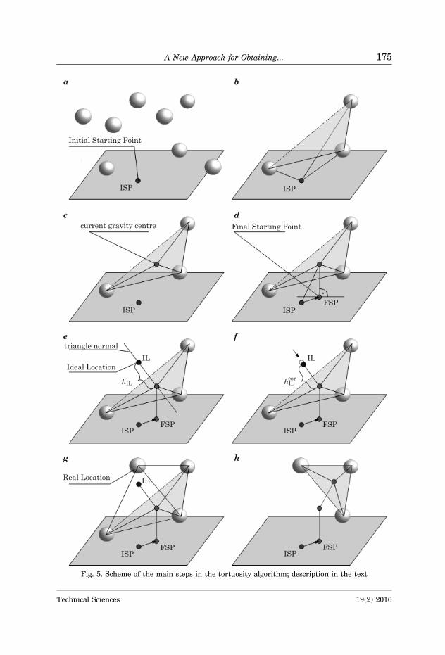
Fig. 5. Scheme of the main steps in the tortuosity algorithm; description in the text



– Find the nearest particle to the IL – this is the Real Location (RL) of the4-th particle forming tetrahedron in the space (g);

– Remove the lowest sphere from tetrahedron 1-2-3-4 to obtain the basetriangle for the next tetrahedron (h);

– Continue the calculations from the third point until reaching the topsurface of the bed;

– Calculate the length of the path inside the tetrahedron (a flow path isa line connecting the centroid of the base triangle with the centroid of one ofthe three side triangles).

The algorithm finishes when the distance between current IL and thenearest particle centre is bigger than the distance between the top surface ofthe bed and the Z coordinate of the IL. The last section is perpendicular to thetop surface of the bed.

The number of path points is higher by two in relation to the number oftetrahedrons used for searching the path sections.

In the PathFinder code an additional algorithm allows to smooth the pathexists. Due to this, the path length is a little shorter. The use of the smoothedvalue is currently not recommended.

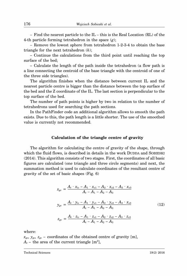
Calculation of the triangle centre of gravity

The algorithm for calculating the centre of gravity of the shape, throughwhich the fluid flows, is described in details in the work DUDDA and SOBIESKI

(2014). This algorithm consists of two stages. First, the coordinates of all basicfigures are calculated (one triangle and three circle segments) and next, thesummation method is used to calculate coordinates of the resultant centre ofgravity of the set of basic shapes (Fig. 6)

xgc =At · xtc – A1 · xs1 – A2 · xs2 – A3 · xs3

At – A1 – A2 – A3

ygc =At · ytc – A1 · ys1 – A2 · ys2 – A3 · xs3 (12)

At – A1 – A2 – A3

zgc =At · ztc – A1 · zs1 – A2 · zs2 – A3 · zs3

At – A1 – A2 – A3

where:xgc, ygc, zgc – coordinates of the obtained centre of gravity [m],At – the area of the current triangle [m2],



xtc, ytc, ztc – coordinates of the current triangle centre [m],A1,2,3 – areas of circle segments [m2],xs, ys, zs – coordinates of gravity centres (denoted by the sign) of circlesegments [m].

Fig. 6. The shape, through which the fluid flows and its gravity centre

The Ideal Location and its correction

For calculating the Ideal Location, a characteristic dimension is used. It canbe the average length of the current triangle sides lave (recommended) or theaverage diameter of spheres dave forming the current triangle. In consecutivecalculations it was assumed, that the tetrahedron is regular and all sides havelengths equal to the characteristic dimension. In that case, the height of suchtetrahedron may be calculated from the simple formula:

hIL = cdim · √2(13)

3

where:hIL – the predicted distance between the IL and the triangle plane [m],cdim – the characteristic dimension [m].

Height hIL is measured on the triangle normal in the direction of increasingvalues of the Z coordinate.

In real systems, particles forming a triangle may not touch one another,which results is that the fourth particle falling partly between them. In



extreme cases, the fourth particle can slide completely between particles thatform the triangle. That can happen when the actual triangle area is three timeslarger than the area of a triangle with one side equal to the average diameter ofthe spheres forming the current triangle (derived in SOBIESKI 2009a). If thisratio is higher than 3, a correction algorithm is used (it may be turned off usingthe settings file) and new three particles close to the current triangle centre arethen searched. The number of such corrected triangles is shown in the finalreport. This normalized critical area of the triangle is also included in thesettings file, but impossible to omit entirely.

Usually the area of the real triangle is far from the critical area and the„sinking” effect is small, but not to omit. Therefore, the formula (13) shouldrather be defined as follows:

hIL = cdim · hcor √2(14)

3

where:hcor is a correction coefficient for the Ideal Location [–].

This coefficient may be defined (in the settings file) as a constant value:

hcor = 0.5 (15)

or a function:

hcor = f(IA) = 1 –exp(a · (IA – b)) (16)

1 + exp(a · (IA – b))

where:IA – the area indicator [–],a – a coefficient (obtained in earlier numerical investigations SOBIESKI

2009a) responsible for the function gradient and equal to 8.0 [–],b – a coefficient (obtained in earlier numerical investigations SOBIESKI

2009a) equal to average value of normalized triangle area for the wholeporous bed, with value equal to 0.5 [–].

The area indicator is defied as

IA =Ai (17)A0



where the current triangle area is calculated from the Heron formula

Ai = √L· (L – a) · (L – b) (L – c) (18)

2 2 2 2

and the area of the reference triangle A0 (triangle with all sides equal to thecharacteristic dimension) as

A0 =cdim · √3 (19)

4

Symbols a, b and c in formula (18) denotes lengths of current triangle sides[m].

The details about this issue as well as the way of obtaining all constants aredescribed in a research report (SOBIESKI 2009a), which was written parallel toperforming implementation actions. This report contains descriptions of manyissues not mentioned in the hereby article and shows the process of creationthe final version of the Path Tracking Method.

Calculating the porosity

Having obtained the information about diameters of all particles in the bed,the total volume of all particles in the porous bed can be calculated. This can bedone as follows:

ns–ns–rej

Vs = Σ π · d3i (20)

6i=1

where:Vs – the total volume of all particles in the bed [m3],di – the diameter of the i-th particle in the bed [m].

Using the formula (8) or (9) and the equation (20), the porosity of thegranular bed may be consequently calculated as:

φ =Vp =

V – Vs = 1 –Vs (21)

V V V



Calculating the inner and the specific surface of the solid body

The inner surface of the solid body may be obtained from the followingformula (assuming point contacts between particles)

ns–ns–rej

Sp = Ss = Σ π · d2i (22)i=1

where:Sp – the total surface of the pore space in the bed [m2],Ss – the total surface of all particles in the bed [m2].

The specific surface of the porous body is calculated in two ways, i.e.according to the Kozeny theory (KOZENY 1927):

S0,Kozeny =Sp (23)V

and to the Carman theory (CARMAN 1997):

S0,Carman =Sp (24)Vs

The relationship between both definitions is as follows:

S0,Kozeny = 1 – φ (25)S0,Carman

The approach to the definition of the specific surface of the porous body isone of the differences between the Kozeny equation and the Carman formula.

Calculation examples

In Table 1 there are settings of PathFinder calculations for the twoexamples previously described. All calculations were made with use of versionIV.1 of the PathFinder code.



Table 1Settings for the calculations in the PathFinder code

Settings Units YADE PFC3D

Number of particles [–] 4000 18188Particle diameter [mm] 31.1 – 57.7 5.5 – 7.5Domain geometry [–] cuboids cylinderISP location [–] 00 00ISP x shift [–] 0.5 0.5ISP y shift [–] 0.5 –Number of rejected particles [–] 0 19Triangle center calculating method [–] gravity centre gravity centreCharacteristic dimension [–] lave lave

Correction method for the IL [–] function functionCorrection coef. for constant method [–] 0.5 0.5a parameter for function method [–] 0.8 0.8b parameter for function method [–] 1.3 1.3Critical area triangle correction [–] Yes YesCritical area of the triangle [–] 3.0 3.0Smooth the path [–] No No

The number of rejected particles ns–rej for performing coarse calculationsshould be set to zero. If there is a suspicion of a free space existence (like in thecase shown in Fig. 3), this value should be increased. The best way to obtainthis parameter is to perform a set of calculations with different ns–rej values andto observe results, particularly the porosity value. A relationship between thenumber of rejected particles and the porosity value may be prepared here (e.g.in a graphical form). On this basis, the best value of this parameter can bechosen. This method was used for obtaining this parameter for the PFC3D

example (SOBIESKI 2009a), in which a free surface of the porous bed exists. Inthe example from YADE, the number of rejected particles equal zero, due tothe way of DEM modelling. All walls were set as flat surfaces, moving closer toeach other during calculations. In such a case, no empty area exists in themodelled system. In the PathFinder software, the ISP must be chosen forperforming the calculations. The simplest way is to choose ISP directly in thesettings file as one from 9 default locations (SOBIESKI 2009a, SOBIESKI et al.2012, SOBIESKI, LIPIŃSKI online). The description of point location contains twosigns (Fig. 7): the first concerns the X axis, the second the Y axis. Both signsmay have values: „–” (the negative part of the axis), „0” (zero point of the axis)and „+” (the positive part of the axis). The combination of signs is as follows:+0, + –, 0 –, – –, –0, – +, 0+, ++, 00.

By default, all points surrounding the zero point of X and Y axis are locatedin the middle of the section connecting the zero point and the domain wall. Thedistance may be changed by using options x-shift and y-shift available in thesettings file. These coefficients may be set between 0 (the ISP is in the zero



point – the middle of the bottom domain wall) and 1 (the ISP is on the wall).The default values for both coefficients are 0.5. This value is not important inthe current point, because only one path, from the central point, is calculated.

Fig. 7. Default locations of the Initial Starting Point for both possible types of domain

In both examples the recommended values for the characteristic dimension(lave), the correction method (function) and its coefficients (a and b), the criticalarea of the triangle, and the method for calculating the triangle centre (gravitycentre) were used.

Table 2 contains the calculation results for both test examples. Thenumbers of path points inform how many of tetrahedral structures were foundin the iteration process. In every structure of this kind, one section of the pathis located. The number of tetrahedral structures is always lowered by 2. Thus

Table 2Results of calculations

Settings Units YADE PFC3D

Number of path points [–] 59 130Number of path rejected points [–] 0 0Number of corrected triangles [–] 0 0Bed (domain) height [m] 0.883302 0.254938Length of the path [m] 1.053803 0.317288Average angle between path sections [o] 141.557825 139.109342Tortuosity [m/m] 1.193026 1.244571Volume of the bed (domain) [m3] 0.345158 0.004505Inner surface of the solid body [m2] 25.534886 2.393343Specific surface (Kozeny def.) [1/m] 73.980321 531.227627Specific surface (Carman def.) [1/m] 127.652558 915.918417Volume of the porous body [m3] 0.200034 0.002613Porosity [m3/m3] 0.420456 0.420006Ergun A [1/m2] 343565.12 16372081.72Ergun 2*B [1/m] 614.39 4248.07Kozeny-Carman term [1/m2] 524013.00 29498873.86



is due to the fact that the first (FSP) and the last path point are calculated indifferent way.

During the calculations, it is checked whether there are duplicate points. Ifyes, one of them is removed from the path and the appropriate information isshown in the final report.

The number of corrected triangles gives information of how many times thecorrections based on critical area of the triangle were made (duplicate pointsmay be created in such case). This value should be zero – other values meanthat in the bed probably a structural non-continuity exists locally. Sometimessuch a case does occur. The importance of other values contained in Table2 has been already explained.

It should be added here, that the B term in the Ergun law is doubled in thefinal report. This is because this term must be introduced in this way in theANSYS Fluent software (Fluent Inc.: Fluent 6.3 User’s Guide, Chapter 7.19:Porous Media Conditions, September 2006, Fluent Inc.: Fluent 6.3 TutorialGuide. September 2006) (but only if the interface is used, not the UDFtechnique).

PathFinder gives possibility to present results of calculation in a graphicalform. The most important visualization may be performed using the ParaViewor MayaVi software. Details about the visualisation processes are described inthe PathFinder User’s Guide (SOBIESKI et al. 2012). In Figure 8 there is theoriginal porous bed created in the PFC3D code (LIU et al. 2008a, b). Additionallythe calculation results of the PathFinder code are visible there and these are:five paths, the spheres surrounding the paths, as well as the tetrahedralstructures used to obtaining the path sections. The tetrahedron structuresmay be additionally coloured according to few scalars: values of triangle areas,values of flow areas, values of perimeters (of the triangle, of the flow shape, andof the friction), values of the quality indicators, values of angles betweentriangle normal and the Z-axis and others. The central path with surroundingspheres and a part of the bed for the YADE example, was shown earlier inFigure 2 (right).

The other way of visualization calculation results is using scripts of theGnuplot graphical environment. Thanks to them, one can follow the process ofcalculation. If appropriate option is set in the settings file, the current resultsmay be shown in every iteration (Fig. 9): the Initial Starting Point, the FinalStarting Point, the current tetrahedron, the current Ideal Location, thecurrent Real Location, the current triangle and the next triangle. At the end,the current path may be shown. When using the Gnuplot scripts, values of allimportant variables may be seen, i.e. those being calculated for every tetrahed-ral structure. Many other Gnuplot scripts are created during such a calcula-tion; most of them are not described here.



Fig. 8. Main forms of visualization of the PathFinder results (PFC3D example)

Fig. 9. Visualization of the first tetrahedron in the path (YADE example)

In the current example, only one path for every case is presented (fromISP = 00) due to the desire to show details of a calculation – some results, likethe number of path rejected points (duplicates) or the number of correctedtriangles must not be averaged. Nevertheless, in general the PathFinder has



appropriate algorithms for automatic calculation of many paths and forcomparing or averaging data. For comparison, the average tortuosity cal-culated for 25 paths (with x-shift and y-shift equal to 0.25, 0.5 and 0.75) isequal to 1.24 for the PFC3D example, and 1.23 for the YADE example. Ingeneral it is recommended to calculate more than one path (minimum 5,SOBIESKI 2009a) and use the average value for further calculations.

Summary

The performed works can be summarized as follows:– The porosity is not a sufficient parameter for describing the spatial

structure of a porous bed. In both examples the porosity values were almost thesame while other properties were different (e.g. the tortuosity).

– A relationship between tortuosity value and the average angle betweenpath sections can be seen. When this angle is smaller, the tortuosity is higher.

– The tortuosity in the PFC3D example is higher than in the second case,which is caused by the differences in the particle sizes and the diameterdistribution. In consequence, the shapes of channels must be more compli-cated. It can be concluded that the tortuosity value depends on the diametersdistribution in the bed.

– The A and B terms are different in both cases. It may stem from the factthat smaller diameters results in turn thinner pore channels. If the porechannel is thinner, the greater is the flow resistance (due to the viscosity).

– The results of calculations described in the article should be comparedwith other methods: analytical (e.g. porosity-tortuosity correlations availablein the literature), numerical (e.g. by the use of the Lattice Boltzmann Methodsor the Immersed Boundary Method) and of course experimental. Such investi-gations are in progress and we will publish their results in the near future.

References

AMAO A.M. 2007. Mathematical Model For Darcy Forchheimer Flow With Applications To WellPerformance Analysis. MSc Thesis. Department of Petroleum Engineering, Texas Tech Univer-sity, Lubbock, Texas.

BELYADI A. 2006. Analysis of Single-Point Test To Determine Skin Factor. PhD Thesis. Department ofPetroleum and Natural Gas Engineering, West Virginia University, Morgantown, West Virginia.

BELYADI F. 2006. Determining Low Permeability Formation Properties from Absolute Open FlowPotential. PhD Thesis. Department of Petroleum and Natural Gas Engineering, West VirginiaUniversity, Morgantown, West Virginia.

CARMAN P.C. 1997. Fluid Flow through a Granular Bed. Transactions of the Institute of ChemicalEngineers, Jubilee Supplement, 75: 32–48.



COMITI J., RENAUD M.A. 1989. New model for determining mean structure parameters of fixed bedsfrom pressure drop measurements: application to beds packed with parallelepipedal particles.Chemical Engineering Science, 44(7): 1539–1545.

DARCY H. 1856. Les Fontaines Publiques De La Ville De Dijon. Victor Dalmont, Paris.DUDDA W., SOBIESKI W. 2014. Modification of the PathFinder algorithm for calculating granular beds

with various particle size distributions. Technical Sciences, 17(2): 135–148.DUNN M.D. 1999. Non-Newtonian Fluid Flow through Fabrics. National Textile Center Annual

Report: C98-P1, Philadelphia University, November.ERGUN S. 1952. Fluid flow through packed columns. Chemical Engineering Progress, 48(2): 89–94.Fluent Inc.: Fluent 6.3 Tutorial Guide. September 2006.Fluent Inc.: Fluent 6.3 User’s Guide, Chapter 7.19: Porous Media Conditions, September 2006.FOURIE W., SAID R., YOUNG P., BARNES D.L. 2007. The simulation of pore scale fluid flow with real

world geometries obtained from X-ray computed tomography. COMSOL Conference, Boston,United States, 14 March.

Gnuplot Home Page. Online: http://www.gnuplot.info/ (access: 1.05.2015).HERNANDEZ A.R.A. 2005. Combined Flow And Heat Transfer Characterization of Open Cell Aluminum

Foams. MSc Thesis. Mechanical Engineering, University Of Puerto Rico, Mayagez Campus, SanJuan, Puerto Rico.

ITASCATM Home Page. Online: http://www.itascacg.com/pfc3d/ (access: 1.05.2015).KOZENY J. 1927. Uber kapillare Leitung des Wassers im Boden. Akademie der Wissenschaften in Wien,

Sitzungsberichte, 136(2a): 271–306.LIU CH., ZHANG Q., CHEN Y. 2008. PFC3D Simulations of lateral pressures in model bin. ASABE

International Meeting, paper number 083340. Rhode Island.LIU CH., ZHANG Q., CHEN Y. 2008. PFC3D Simulations of vibration characteristisc of bulk solids in

storage bins. ASABE International Meeting, paper number 083339. Rhode Island.LORD D.L., RUDEEN D.K., SCHATZ J.F., GILKEY A.P., HANSEN C.W. 2006. DRSPALL: Spallings Model for

the Waste Isolation Pilot Plant 2004 Recertification. SAND2004-0730, Sandia National Labora-tories, Albuquerque, New Mexico, Livermore, California.

MIAN M.A. 1992. Petroleum engineering handbook for the practicing engineer. Pennwell Publishing,Tulsa, Oklahoma.

NEETHIRAJAN S., KARUNAKARAN C., JAYAS D.S., WHITE N.D.G. 2006. X-ray Computed TomographyImage Analysis to explain the Airflow Resistance Differences in Grain Bulks. Biosystems Engin-eering, 94(4): 545–555.

NIVEN R.K. 2002. Physical insight into the Ergun and Wen and Yu equations for fluid flow in packedand fluidised beds. Chemical Engineering Science, 57(3): 527–534.

ParaView Home Page. Online: http://www.paraview.org/ (access: 1.05.2015).RAINEY T.J., DOHERTY W.O.S., BROWN R.J., KELSON N.A., MARTINEZ D.M. 2008. Determination of the

permeability parameters of bagasse pulp from two different sugar extraction methods. TAPPIEngineering, Pulping & Environmental Conference. Portland, Oregon, United States, August24–27.

RESCH E. 2008. Numerical and Experimental Characterisation of Convective Transport in Solid OxideFuel Cells. MSc Thesis, Queens University, Kingston, Ontario, Canada.

ROSSEL S.M. 2004. Fluid flow modeling of resin transfer molding for composite material wind turbineblade structures. Sandia National Laboratories on-line report no SAND04-0076. Department ofChemical Engineering, Montana State University – Bozeman, Bozeman, Montana.

SAMSURI A., SIM S.H., TAN C.H. 2003. An Integrated Sand Control Method Evaluation. Society ofPetroleum Engineers, SPE Asia Pacific Oil and Gas Conference and Exhibition, Jakarta,Indonesia, 9–11 September.

SKJETNE E., KLOV T., GUDMUNDSSON J.S. 1999. High-Velocity Pressure Loss In Sandstone Fractures:Modeling And Experiments (SCA-9927). International Symposium of the Society of Core Analysts,Colorado School of Mines, Colorado, August 1–4.

SOBIESKI W. 2009a. Calculating tortuosity in a porous bed consisting of spherical particles with knownsizes and distribution in space. Research report 1/2009, Winnipeg.



SOBIESKI W. 2009b. Switch Function and Sphericity Coefficient in the Gidaspow Drag Model forModeling Solid-Fluid Systems. Drying Technology, 27(2): 267–280.

SOBIESKI W. 2010. Examples of Using the Finite Volume Method for Modeling Fluid-Solid Systems.Technical Sciences, 13: 256–265.

SOBIESKI W. 2014. The quality of the base knowledge in a research process. Scientific researches in thedepartment of mechanics and machine design, University of Warmia and Mazury in Olsztyn, 2:29–47.

SOBIESKI W., LIPINSKI S. The PathFinder User’s Guide. Online: http://www.uwm.edu.pl/pathfinder/(access: 1.05.2015).

SOBIESKI W., TRYKOZKO A. 2011. Sensitivity aspects of Forchheimer’s approximation. Transport inPorous Media, 89(2): 155–164.

SOBIESKI W., TRYKOZKO A. 2014a. Forchheimer Plot Method in Practice. Part 1. The experiment.Technical Sciences, 17(4): 221–335.

SOBIESKI W., TRYKOZKO A. 2014b. Forchheimer Plot Method in Practice. Part 2. A numerical model.Technical Sciences, 17(4): 337–350.

SOBIESKI W., ZHANG Q., LIU C. 2012. Predicting Tortuosity for Airflow Through Porous Beds Consistingof Randomly Packed Spherical Particles. Transport in Porous Media, 93(3): 431–451.

The MayaVi Data Visualizer. Online: http://mayavi.sourceforge.net/index.html (access: 1.05.2015).The PathFinder Project. Online: http://www.uwm.edu.pl/pathfinder/ (access: 1.05.2015).WHITAKER S. 1996. The Forchheimer equation: A theoretical development. Transport in Porous Media,

25(1): 27–61.WU J., YU B., YUN M. 2008. A resistance model for flow through porous media. Transport in Porous

Media, 71(3): 331–343.



A NEW APPROACH FOR OBTAINING THE GEOMETRIC PROPERTIES OF · PDF fileA NEW APPROACH FOR...

Documents

Transcript of A NEW APPROACH FOR OBTAINING THE GEOMETRIC PROPERTIES OF · PDF fileA NEW APPROACH FOR...