Research Article

716

Received: 5 September 2008, Revised: 21 January 2009, Accepted: 30 January 2009, Published online in Wiley InterScience: 10 July 2009

(www.interscience.wiley.com) DOI:10.1002/nbm.1383

A multivariate hypothesis testing framework for tissue clustering and classification of DTI data Raisa Z. Freidlina*, Evren Ozarslanb, Yaniv Assafc, Michal E. Komloshb

and Peter J. Basserb

AbstractThe primary aim of this work is to propose and invest

NMR Biom

igate the effectiveness of a novel unsupervised tissue clustering and classification algorithm for diffusion tensor MRI (DTI) data. The proposed algorithm utilizes information about the degree of homogeneity of the distribution of diffusion tensors within voxels. We adapt frameworks proposed by Hext and Snedecor, where the null hypothesis of diffusion tensors belonging to the same distribution is assessed by an F-test. Tissue type is classified according to one of the four possible diffusion models, the assignment of which is determined by a parsimonious model selection framework based on Schwarz Criterion. Both numerical phantoms and diffusion-weighted imaging (DWI) data obtained from excised rat and pig spinal cords are used to test and validate these tissue clustering and classification approaches. The unsupervised clustering method effectively identifies distinct regions of interest (ROIs) in phantoms and real experimental DTI data. Copyright © 2009 John Wiley & Sons, Ltd.

Keywords: DTI; diffusion tensor; tissue; region growing; clustering; segmentation; classification; hypothesis testing; ROI; DWI; F-test

a R. Z Freidlin Biomedical Imaging and Visualization Section, Computational Bioscience and Engineering Laboratory, Division of Computational Bioscience, Center for Information Technology, National Institutes of Health, Bethesda, Maryland 20892, USA

b E. O zarslan, M. E Komlosh, P. J Basser Section on Tissue Biophysics and Biomimetics, Laboratory of Integrative and Medical Biophysics, National Institute of Child Health and Human Development, National Institutes of Health, Bethesda, Maryland 20892, USA

c Y. Assaf Department of Neurobiochemistry, Tel Aviv University, Ramat Aviv, Israel

* Correspondence to: R. Z Freidlin, Biomedical Imaging and Visualization Section, Computational Bioscience and Engineering Laboratory, Division of Computational Bioscience, Center for Information Technology, National Insti­tutes of Health, Bethesda, Maryland 20892, USA. E-mail: raisa@helix.nih.gov

Abbreviations used: DT-MRI or DTI, diffusion tensor magnetic resonance imaging; DWI, diffusion-weighted imaging; FA, fractional anisotropy; RA, relative anisotropy; ROI, region of interest; RSS, residual sum of squares; SC, Schwarz criterion; SNR, signal to noise ratio; Tr, trace of the diffusion tensor.

INTRODUCTION

Diffusion tensor magnetic resonance imaging (1) (DT-MRI or DTI) provides noninvasive quantitative measurements of the apparent diffusion tensor of water molecules in tissue. In an anisotropic medium, the signal attenuation in diffusion-weighted images depends on the underlying tissue structure and is affected by many complex factors. For instance, in brain white matter, the diffusion-weighted imaging (DWI) signal is affected by the fiber orientation, the organization and architecture of myelinated axons within fascicles (2), and the distribution of fiber diameters and densities, etc. The diffusion tensor’s eigenvalues are the principal diffusivities that indicate the degree of symmetry of the underlying diffusion process; their corresponding eigenvectors determine the orientation of the principal axes. In recent years, DTI has been widely used in medicine.

Therefore, it has become increasingly important to be able to differentiate between tissue structures, both to address basic biological development of tissues and organs and to improve therapies and diagnostics. Diffusion image segmentation and classification are one of the methods to achieve these goals. Most of the work in DTI segmentation is based on applying thresholding criteria to tensor-derived scalar quantities, such as the trace of the diffusion tensor (Tr), the fractional anisotropy (FA), and the relative anisotropy (RA). Some algorithms combine the FA scalar index with the fiber orientation of tissue (3–6) or T2-weighted image data (7). However, these scalars are generally subject to bias usually due to background noise (8,9). Zhukov et al. (10) introduced a new anisotropy measure invariant for segmenting regions and refining with a level set method. However, this approach is still based on a scalar measure, which neglects the orientation of the diffusion tensor. Li et al. (11) suggested a multiscale statistical classification and partial volume

ed. 2009; 22: 716–729 Copyright © 2009

voxel reclassification method, in which segmentation is per­formed in multiple stages on a stack of images at different levels of inner spatial scale. In recent years, a number of segmentation approaches using

the full diffusion tensor (12) have been introduced by Feddern et al. (13), Wiegell et al. (14), Wang et al. (15,16), Rousson et al. (17), Lenglet et al. (18,19), and Jonasson et al. (20). Alexander et al. (21) concluded that the Euclidean difference measure performs the best for matching diffusion tensors. In Reference (13), this measure was used along with level set methods, such as mean curvature motion and self-snakes and extended to a classical

John Wiley & Sons, Ltd.

TISSUE CLUSTERING AND CLASSIFICATION OF DTI DATA

1Given two vectors P and V, the element-wise exponentiation is defined as P=e V, where Pi ¼ eVi . 7

geodesic active contour model for segmentation and regular­ization of tensor-valued images. Wiegell et al. (14) applied the modified k-means algorithm for unsupervised clustering of thalamic nuclei with the distance metric specified by a linear combination of the Mahalanobis and the Euclidean distance between tensors defined by the Frobenius tensor norm. The Euclidean distance between two tensors incorporated into an active contour model to segment diffusion tensor data was also used by Wang et al. (15). In Reference (17), the surface evolution method was extended by incorporating region statistics of the full tensor for segmenting DTI data. A new measure of dissimilarity between tensors was later introduced by Wang et al. (16,22) and is based on symmetrized Kullback–Leibler divergence. This concept was further extended by Lenglet et al. (18) for 3D probability density field segmentation with higher internal variance. Subsequently, Lenglet et al. (19) and Awate et al. (23) employed Riemannian tensor metrics for image segmenta­tions by estimating tensor statistics in fiber bundles using parametric and nonparametric techniques, respectively. Spectral clustering, based on a graph partitioning, was successfully used by Ziyan et al. (24) to segment thalamic nuclei. Multivariate statistical tests for group-wise DTI statistical analysis were used by Khurd et al. (25) and Whitcher et al. (26).

In this work we propose a novel approach, based on multivariate statistical hypothesis F-testing (27,28), for assessing similarities between entire tensors in different voxels in order to perform unsupervised tissue clustering on diffusion tensor data. The advantages of using statistical hypothesis testing are numerous. One lies in performing tests on the entire diffusion tensor, which contains information about Tr, FA, and diffusion orientation. Another advantage is that one can assess errors in region of interest (ROI) selection and choose confidence levels for each test. A third advantage is its computational efficiency. These tests are rapid, easy to implement, and can be performed on a voxel-by-voxel basis. There are several differences between our approach (29,30)

and the previously described methods. First, the algorithm we propose does not require continuity of the segmented regions, nor does it employ specific distance metrics in tensor space and thus does not rely on any parameter setting/tuning prior to and/ or during clustering. However, the assumptions of normally distributed residuals and homoscedasticity (i.e. uniformity of the variance within ROIs) have to be satisfied in order to perform hypothesis testing (31). Second, in comparison with the k-means clustering approach, the proposed method has no prerequisites for assigning the number of clusters or their initial centroids. Classification is based on the diffusion properties of the seed voxels, which have been determined by a hierarchical parsimo­nious model selection framework (31), using the Schwarz Criterion (32), also known as the Bayesian Information Criterion. This paper is organized as follows: The Theory section provides

a background on diffusion tensor imaging and introduces the framework for multivariate hypothesis testing. In the Clustering Based on the Parametric Distribution of Diffusion Tensors section, we describe the clustering approach, which is based on a parameter distribution of diffusion tensors and a step-by-step selection of a seed region. The Methods section contains information about simulated and experimental data used for validation and in the Results section, we present results obtained with our clustering method. Finally, in the Discussion and Conclusion sections we discuss the pros and cons of the proposed method.

NMR Biomed. 2009; 22: 716–729 Copyright © 2009 John Wiley

THEORY

Diffusion tensor imaging

Diffusion tensor imaging describes water diffusion in tissues by analyzing the relationship between the signal loss (12,33), caused by the random motion of water molecules along diffusio­n-encoding gradients applied in various directions, and the apparent diffusion tensor, D:

-trðbDÞSðGÞ ¼ Sð0Þe (1)

where S(G) is the observed signal attenuated by the diffusion-weighting gradient G ¼ (Gx, Gy, Gz), S(0) is the signal in the absence of the diffusion-weighting gradient, and b is the b-matrix computed by

[ ]d

bij ¼ g 2GiGj d2 D - (2)

3

where Gi is the component of the diffusion gradient along one of the coordinate axes (i ¼ x, y, or z) with duration d, and D is the diffusion time. In eqn (1) D is a symmetric (3 x 3) second-order diffusion tensor (12). We reformat D as a column vector that contains the elements of the estimated diffusion tensor as follows:

D ¼ Dxx ; Dyy ; Dzz ; Dxy ; Dxz ; Dyz (3) T

where diagonal elements, Dxx, Dyy, and Dzz are the apparent diffusivities along xx, yy, and zz directions, while the remaining (off-diagonal) elements represent correlations in displacements along orthogonal directions. These six independent elements are sufficient to describe Gaussian molecular diffusion in three dimensions.

Parameter estimation framework for multivariate hypothesis testing

To estimate the diffusion tensor from the function in eqn (1), we applied a nonlinear least-square minimization method, proposed by Koay et al. (34), for which the initial guesses were obtained using linear least-squares minimization:1

-BCSðGÞ ¼ e (4)

where n is a number of DWI acquisitions, S is the (n x 1) vector of the observed signal values, B is the (n x 7) design matrix, which consists of a list of (1 x 6) b-matrix elements and (-1) for a series of n DWI acquisitions:

2 3b2 b2 b2 -1 x1 y1 z1

2bx1y1 2bx1 z1 2by1z1b2 b2 -1 76 b2 6 x2 y2 z2

2bx2y2 2bx2 z2 2by2z2 776 ......

......

......

...B ¼ (5)6 76 76 ......

......

......

...754

b2 b2 b2 2bxnyn 2bxnzn 2bynzn -1xn yn zn

and C is a (7 x 1) column vector that contains the estimated diffusion tensor and log[S(0)]:

TC ¼ Dxx ; Dyy ; Dzz ; Dxy ; Dxz; Dyz ; log½Sð0Þ (6)

www.interscience.wiley.com/journal/nbm & Sons, Ltd.

17

R. Z. FREIDLIN ET AL.

718

The residual sum of squares (RSS) is estimated according to

n X( )2-Bi CRSS ¼ SiðGÞ - e (7) i¼1

where Bi is the ith row of B, S -Bi Ci(G), e are the observed and

estimated signals respectively, and n is the number of diffusion-weighted acquisitions.

CLUSTERING BASED ON THE PARAMETRIC DISTRIBUTION OF DIFFUSION TENSORS

In this work we propose a novel tissue clustering algorithm based on the multivariate F-test for grouping voxels with the same distribution of diffusion tensor parameters. In order to justify the use of this hypothesis testing framework, the assumptions of normally distributed residuals and homoscedasticity (i.e. uniform­ity of the variance within an ROI) have to be satisfied. It has previously been shown that the residuals are asymptotically normally distributed (35) at SNR greater than 7 in an experiment otherwise free of systematic artifacts. However, in the same work, Carew et al. (35) also reported that the variance in the voxels with different fractional anisotropies, FAs2, may not be homogeneous (in particular, voxels with low FA have higher estimated variance in FA than voxels with high FA), thus violating the assumption of variance uniformity. To overcome this problem in the proposed clustering approach, the seed region is selected from one of the three anisotropic models, i.e. general anisotropic (l1 > l2 > l3), oblate (l1 ¼ l2 > l3), or prolate (l1 > l2 ¼ l3), thus the voxels included in the seed region are presumed to have an FA greater than 0.5. These models are identified by a previously proposed parsimonious model selection framework (31), using the Schwarz Criterion (32). This framework selects the diffusion model (general anisotropic, prolate, oblate, or isotropic) that best fits the DWI data using the fewest number of parameters, by imposing penalties for models with a larger number of free parameters. It is defined as

( )RSSk logðnÞ

SCk ¼ log þ dk (8) n n

where k represents the model type (general anisotropic, prolate, or oblate), n is the number of experimental data points, and d is the number of free parameters for the kth model (d is set to 7 and 5 for the general anisotropic and prolate/oblate models, respectively). Once the optimal model is chosen in each voxel, m neighboring seed voxels are picked within the same model type (as described below), i.e. having similar FA values, to satisfy the assumption that the variance of each measurement in the seed region is uniform (homoscedasticity), and that the distributions of diffusion tensor parameters are similar. Testing voxels of interest against such homogeneous seed regions makes the unsupervised clustering algorithm more reliable.

Choosing a seed region

The first step in selecting a seed region is to perform a voxel-by-voxel search until m neighboring voxels (e.g. 6–9 voxels in a [3 x 3] sector) of the same model type (general anisotropic,

2

rffiffiffiffiffiffiffiffiffiffiffiffiffiffiffiffiffiffiffiffiffiffiffiffiffiffiffiffiffiffiffiffiffiffiffiffiffiffiffiffiffiffiffiffiffiffiffiffiffiffiffiqffiffiÞ23 ðl1-hliÞ2þðl2-hliÞ2þðl3-hliFA ¼ 2 l2þl2þl2; where hli ¼ ðl1 þ l2 þ l3 Þ=3

1 2 3

www.interscience.wiley.com/journal/nbm Copyright © 200

oblate, or prolate) are located. The null hypothesis, which assumes that the distributions of diffusion tensor parameters in these m voxels are the same, is tested by taking the following steps, adapted from Hext (28) (see Fig. 1):

(1) C

Figable

9 Jo

ombine m sets of [n x 1] acquired signals, Si(G), into [n · m x 1] array, SCAS, where n is the number of experimental data points in each voxel and i ¼ 1, 2,. . ., m.

(2) C

ombine m sets of individually estimated signals, e- BCi , into [n · m x 1] array, SCES, where n is the number of experimental data points in each voxel and 1, 2,. . .,m.

(3) E

stimate the RSS for the combined individually estimated signals, RSSCES, by

n·mXÞ2

i¼1

RSSCES ¼ ðSCASi - SCESi

(4) E

stimate CAvg for all m voxels using the combined acquired signals, SCAS, and the augmented [n · m x 7] design matrix, BC,

ure 1. Schematic diagram of the algorithm flow. This figure is avail­ in color online at www.interscience.wiley.com/journal/nbm

hn Wiley & Sons, Ltd. NMR Biomed. 2009; 22: 716–729

TISSUE CLUSTERING AND CLASSIFICATION OF DTI DATA

3A t(27)

nes

NM

as described in the Parameter Estimation Framework for Multivariate Hypothesis Testing subsection.

(5) E

stimate the average [n ·m x 1] signal vector, SAvg, using

^S -BC CAvgAvgðGÞ ¼ e .

(6) E

stimate the RSS for the average signal, RSSAvg, by

n·m X ( )2RSSAvg ¼ SCASi - SAvgi

i¼1

(7) A

Table 1. FA and Tr ( x10-6mm2 /s) values for the oblate and prolate regions in synthetic phantoms with different degrees of oblateness and prolateness

Region # Diffusion model FA Tr

’Lower’ FAs 1 Oblate 0.53 3100 2 0.48 3300 3 0.58 3800 4 0.62 3300 5 Prolate 0.7 2100 6 0.62 2300

pply the F-test, adapted from Snedecor3, on the null hy­pothesis to assess the similarity among variances within the voxels:

ðRSSAvg - RSSCESÞ=ðfp · ðm - 1ÞÞ F0 ¼ (9)ðRSSCESÞ=ðm · ðn - fpÞÞ

where fp ¼ 7 is the number of free parameters in the general anisotropic model, m is a number of voxels with n experimental data points each. The null hypothesis that the diffusion tensors in all m voxels

belong to the same parametric distribution is accepted if

F0 < Fð1 - a; n1; n2Þ (10)

where Fð1 - a; n1; n2Þ is the critical value from the F distribution with n1 ¼ fp · ðm - 1Þ and n2 ¼ m · ðn - fpÞ degrees of freedom and a significance level of a. If eqn (10) is satisfied, these voxels will be used as a seed region for subsequent clustering. Otherwise, the algorithm moves to the next voxel and repeats Steps 1 through 7 above.

Clustering

Clustering is performed by testing each voxel in the image against the seed region. The new null hypothesis assumes that the distributions of diffusion tensor parameters in the tested voxel and in the m seed voxels are the same. To test null hypothesis, Steps 1 through 7, as in the previous section, are repeated. However, the combined set now consists of m þ 1 voxels, where m are voxels in the seed regions. If the F0 value in eqn (9) for m þ 1 voxels is small, the null hypothesis, that the diffusion tensor parameters in the tested voxel are the same as in the seed region, is accepted and the voxel is added to the cluster. Once all voxels are tested against given seed regions, the next

seed region is selected according to the steps in the previous section (previously clustered voxels are excluded from all future tests). The clustering process stops when no new seed regions can be identified.

7 0.78 2300 8 0.83 1900 — General anisotropic 0.55 2500 — Isotropic 0.05 2200

’Higher’ FAs 1 Oblate 0.59 3300 2 0.54 3500 3 0.64 3900 4 0.68 3500 5 Prolate 0.8 2100 6 0.72 2300

METHODS

Simulations

To evaluate the unsupervised clustering approach, synthetic phantoms were generated in MATLAB (The MathWorks, Inc.) by setting the signal-to-noise ratio, SNR, in S(0) images to 20, 25, and 33 (the latter matches the SNR in the excised pig spinal cord DTI data), for a fixed signal intensity, I0 ¼ 1000. White matter was simulated with the general anisotropy and prolate models, while

ypographical error appears in Statistical Methods by Snedecor and Cochran in the formula given on page 344 describing the F-test comparing two ted models. The corrected formula is given in eqn (9).

R Biomed. 2009; 22: 716–729 Copyright © 2009 John Wiley

gray matter was simulated with the isotropic model with values typical for living brain tissue (36). The oblate model was set to parameters between white and gray matter. The confidence interval for an F-test was set to 95%.

Synthetic phantoms with different degrees of oblateness and prolateness

For each SNR, two phantoms with ‘Lower’ FAs and ‘Higher’ FAs for the oblate and prolate regions were simulated (Table 1). Normally distributed random noise was added to the signal

intensity in each voxel to make the diffusion-weighted images Rician distributed according to the following equation:

qffiffiffiffiffiffiffiffiffiffiffiffiffiffiffiffiffiffiffiffiffiffiffiffiffiffiffiffiffiffiDWI ¼ DWI2 þ DWI2 (11)Re Im

where

-trðbDÞ þ NRe;DWIRe ¼ I0e DWIIm ¼ NIm

and NRe and NIm are normally distributed random numbers with mean zero and standard deviation s ¼ I0/SNR. This model assumes that noise is added to the real and imaginary channels independently, and that the MR signal is rectified (9,37).

Synthetic phantoms with different spatial orientations

To evaluate the ability of the proposed clustering method to discriminate between tensors with different spatial orientations, we simulated a number of phantoms with fixed FA and Tr values and SNRs set to 20, 25, and 33, where noise was added as before. However, in these simulations, the diffusion tensors in the oblate

7 0.88 23008 0.92 1900 — General anisotropic 0.62 2600— Isotropic 0.06 2200

& Sons, Ltd. www.interscience.wiley.com/journal/nbm

719

R. Z. FREIDLIN ET AL.

Table 2. FA and Tr (x10 -6mm 2/s) values for the syntheticphantoms with different spatial orientations

Region #

Diffusion model FA Tr u (8)

’Lower’ FAs 1 Oblate 0.53 3100 0 2 9 3 184 275 Prolate 0.7 2100 0 6 9 7 188 27— General

anisotropic 0.5 2500 0

— Isotropic 0.05 2200 0 ’Higher’ FAs

1 Oblate 0.59 3300 0 2 9 3 184 275 Prolate 0.8 2100 0 6 9 7 188 27— General

anisotropic 0.62 2600 0

— Isotropic 0.06 2200 0

720

and prolate regions were rotated from the z-axis as described in Table 2.

Synthetic phantoms with partial volumes

The synthetic phantoms with partial volume regions between the prolate quadrants (corresponding parameters are shown in Table 3) were generated in order to evaluate the capability of the clustering algorithm to identify voxels affected by partial voluming. Partial volume regions were simulated according to

- -trðbDj ÞtrðbDi Þ þ ð1 - f Þ · Sð0ÞSðGÞ ¼ f · Sð0Þe e ; for i 6¼ j (12)

where Di and Dj are the diffusion tensors (prolate model) with different degrees of prolateness and f is the volume fraction coefficient ( f < 1), which continuously changes from one cluster to its neighbor.

Table 3. FA and Tr ( x10-6mm 2/s) values for the synthetic phantoms of prolate models with partial volumes

5 6 7 8

FA 0.8 0.85 0.87 0.9 Tr 2100 2000 2400 2000 u (8) 0 60 20 40

www.interscience.wiley.com/journal/nbm Copyright © 200

For all simulated phantoms, the b-matrix was calculated with the imaging parameters described in the Excised Pig Spinal Cord DTI Experiments subsection. The unsupervised clustering algorithm was applied to the set

of 46 reconstructed diffusion-weighted images with four nondiffusion-weighted images (b " 0 s/mm2). The confidence interval for an F-test was set to 99%.

Excised spinal cord DTI experiments

In addition to the numerical simulations, we tested our method on experimental MRI data obtained from excised rat and pig spinal cords fixed with a 4% paraformaldehyde solution. Prior to MR data collection, the spinal cord was washed in phosphate-buffered saline (PBS) to avoid signal loss due to fixative-related T2-shortening (38). The p-value of 0.05 was used for all tests.

Excised rat spinal cord DTI experiments

DWIs were obtained using a diffusion-weighted stimulated echo pulse sequence with d (pulse duration) ¼ 2.5 ms, D (diffusion time) ¼ 70 ms, TR ¼ 3500 ms, and TE¼ 14.7 ms on a horizontal-bore 7T scanner equipped with a Micro2.5 microscopy probe with a maximal gradient strength of 1460 mT/m (Bruker, Germany). Other imaging parameters were: in-plane resolution 200 x 200 mm2, slice thickness ¼ 2 mm, number of averages (NEX) ¼ 3, bandwidth ¼ 50 kHz. For seven slices, 40 DWIs per slice were acquired during 28 h of scanning. Thirty-one of these were attenuated by diffusion gradients G ¼ (Gx, Gy, Gz) and nine were not attenuated ( j jG ¼ 0). In each direction the approximate b-value was 2000 s/mm2. The SNR for this experiment was 31.

Excised pig spinal cord DTI experiments

The sample was imaged in a 15 mm NMR tube containing MR-compatible perfluoropolyether oil (‘Fomblin’), using a Micro2.5 microscopy probe (15 mm solenoid coil) with 1450 mT/m 3-axis gradients (7T vertical-bore MRI scanners, Bruker, Germany). A diffusion-weighted spin echo pulse sequence was used with TR ¼ 3500 ms, TE ¼ 33 ms, band­width ¼ 50 kHz, in-plane resolution 94 x 94 mm2 with seven continuous 1 mm thick slices. Four DWIs per slice were acquired without applying the diffusion sensitizing gradients (b " 0 s/ mm2), followed by the acquisition of 46 diffusion-weighted images with diffusion gradient strength (G) ¼ 120 mT/m yielding approximate b-values of 1000 s/mm2. The number of averages (NEX) was 2. Each of these diffusion-weighted scans was collected with diffusion gradients applied along a different direction determined from the second-order tessellations of an icosahe­dron on the surface of a unit hemisphere. The diffusion gradient duration (d) was 5 ms, and the gradient separation (D) was 20 ms. The total imaging time was less than 13 h (SNR ¼ 33). At each voxel location in the raw rat and pig spinal cord images,

the apparent diffusion tensor, D, was calculated (12). Tensor-derived parameters, such as the Tr, FA, the eigenvectors, e1, e2, and e3, and the eigenvalues, l1, l2, and l3, were all calculated and passed to the parsimonious model selection algorithm and, subsequently, to the clustering method, based on the multi­variate hypothesis testing.

9 John Wiley & Sons, Ltd. NMR Biomed. 2009; 22: 716–729

0

50

(a) (b)QQ Plot of Sample Data versus Standard Normal QQ Plot of Sample Data versus Standard Normal 150 3000

100 2000

Qua

ntile

s of

Inpu

t Sam

ple

−50 Qua

ntile

s of

Inpu

t Sam

ple 1000

0

−1000

−100 −2000

−4 −150

−3 −2 −1 0 1

Standard Normal Quantiles

2 3 4 −5 −3000

−4 −3 −2 −1 0 1

Standard Normal Quantiles

2 3 4 5

721

TISSUE CLUSTERING AND CLASSIFICATION OF DTI DATA

Figure 2. Q–Q plot of residuals in (a) phantom and (b) pig spinal cord versus standard normal.

Figure 3. Synthetic phantom generated with different degrees of oblateness in regions #1–4 and prolateness in regions #5–8 (‘Lower’ FAs in Table 1) at SNR ¼ 33: (a) the fractional anisotropy and (b) trace (mm2/s) maps; (c) color-coded parsimonious model map (blue–isotropic, orange–oblate, red–prolate, and turquoise–general anisotropic models); (d) identified oblate and prolate clusters (colors depict different clusters and are not related to colors in the parsimonious model map). This figure is available in color online at www.interscience.wiley.com/journal/nbm

NMR Biomed. 2009; 22: 716–729 Copyright © 2009 John Wiley & Sons, Ltd. www.interscience.wiley.com/journal/nbm

R. Z. FREIDLIN ET AL.

722

RESULTS

The residuals from the phantom and the excised rat and pig spinal cord experiments (SNR ¼ 33) are asymptotically normally distrib­uted (Fig. 2) and the variance of each measurement is presumed to be unchanging (homoscedasticity), thus testing one model against another, in the manner presented below, is well grounded.

Simulations

Synthetic phantoms with different degrees of oblateness and prolateness

Figure 3a and b shows the FA and Tr maps for the simulated phantoms at SNR ¼ 33, which corresponds to the SNR in the acquired images of an excised pig spinal cord. Although, from these figures it might seem obvious visually that there are four distinct domains in both oblate and prolate regions, such visual delineation is possible only by placing all voxels with equal FAs and Trs in homogeneous ROIs. Otherwise, variations in FA from 0.5 to 0.6 in the oblate regions and 0.7 to 0.8 in the prolate regions, with Tr differences only around 300 x 10 -6 mm2/s, would not be visible. The parsimonious model selection results

Figure 4. Performance comparison for the oblate and prolate regions at (a) Sby the darker bar and ‘Higher’ FAs by the lighter bar. The true positive countspositive counts are obtained from the outside regions.

www.interscience.wiley.com/journal/nbm Copyright © 200

(Fig. 3c) had 97% success of identifying correct models. However, from these results it is not obvious that both oblate and prolate regions consist of distinct quadrants. In contrast, the proposed clustering algorithm correctly identified regions with different degrees of oblateness and prolateness (Table 1), which are shown in Fig. 3d. The general anisotropic area was clustered with 100% success (results are not shown in this paper). The isotropic voxels with FA¼ 0.2 (depicted in blue in Fig. 3c) remained unclustered with 100% success.

Performance evaluation of the clustering algorithm at different SNRs and FAs for the oblate and prolate regions is shown in Fig. 4. Overall, the proposed method performed better for the FA values greater than 0.55 at all SNRs. The same behavior was observed in the prolate regions. However, the performance of clustering significantly decreased at FA < 0.5 and SNR < 25 in the oblate area, i.e. regions #1 and #2 were merged together. All voxels in the general anisotropic region at all SNRs were clustered correctly.

Synthetic phantoms with different spatial orientations

As can be seen from Fig. 5a, b, and c, oblate and prolate regions appear homogeneous in the FA, Tr, and parsimonious model

NR ¼ 33; (b) SNR ¼ 25; and (c) SNR ¼ 20, where ‘Lower’ FAs are represented are calculated within the areas of corresponding clusters, while the false

9 John Wiley & Sons, Ltd. NMR Biomed. 2009; 22: 716–729

TISSUE CLUSTERING AND CLASSIFICATION OF DTI DATA

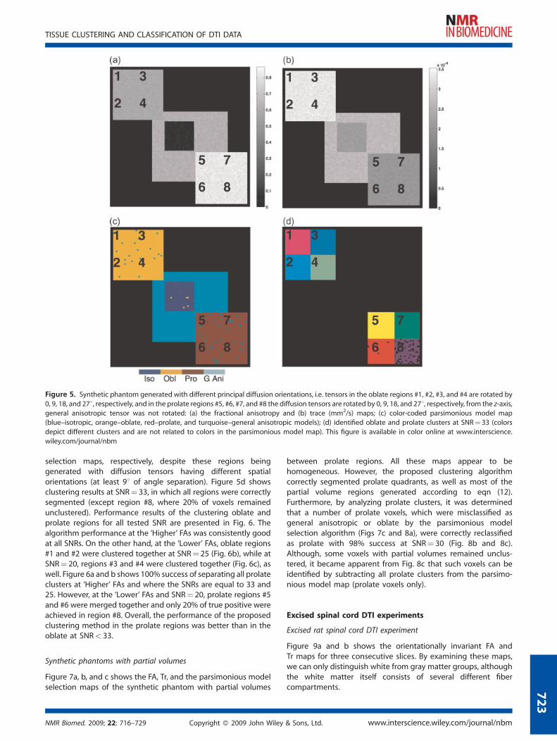
Figure 5. Synthetic phantom generated with different principal diffusion orientations, i.e. tensors in the oblate regions #1, #2, #3, and #4 are rotated by 0, 9, 18, and 278, respectively, and in the prolate regions #5, #6, #7, and #8 the diffusion tensors are rotated by 0, 9, 18, and 278, respectively, from the z-axis, general anisotropic tensor was not rotated: (a) the fractional anisotropy and (b) trace (mm2/s) maps; (c) color-coded parsimonious model map (blue–isotropic, orange–oblate, red–prolate, and turquoise–general anisotropic models); (d) identified oblate and prolate clusters at SNR ¼ 33 (colors depict different clusters and are not related to colors in the parsimonious model map). This figure is available in color online at www.interscience. wiley.com/journal/nbm

7

selection maps, respectively, despite these regions being generated with diffusion tensors having different spatial orientations (at least 98 of angle separation). Figure 5d shows clustering results at SNR ¼ 33, in which all regions were correctly segmented (except region #8, where 20% of voxels remained unclustered). Performance results of the clustering oblate and prolate regions for all tested SNR are presented in Fig. 6. The algorithm performance at the ‘Higher’ FAs was consistently good at all SNRs. On the other hand, at the ‘Lower’ FAs, oblate regions #1 and #2 were clustered together at SNR ¼ 25 (Fig. 6b), while at SNR ¼ 20, regions #3 and #4 were clustered together (Fig. 6c), as well. Figure 6a and b shows 100% success of separating all prolate clusters at ‘Higher’ FAs and where the SNRs are equal to 33 and 25. However, at the ‘Lower’ FAs and SNR ¼ 20, prolate regions #5 and #6 were merged together and only 20% of true positive were achieved in region #8. Overall, the performance of the proposed clustering method in the prolate regions was better than in the oblate at SNR < 33.

Synthetic phantoms with partial volumes

Figure 7a, b, and c shows the FA, Tr, and the parsimonious model selection maps of the synthetic phantom with partial volumes

NMR Biomed. 2009; 22: 716–729 Copyright © 2009 John Wiley

between prolate regions. All these maps appear to be homogeneous. However, the proposed clustering algorithm correctly segmented prolate quadrants, as well as most of the partial volume regions generated according to eqn (12). Furthermore, by analyzing prolate clusters, it was determined that a number of prolate voxels, which were misclassified as general anisotropic or oblate by the parsimonious model selection algorithm (Figs 7c and 8a), were correctly reclassified as prolate with 98% success at SNR ¼ 30 (Fig. 8b and 8c). Although, some voxels with partial volumes remained unclus­tered, it became apparent from Fig. 8c that such voxels can be identified by subtracting all prolate clusters from the parsimo­nious model map (prolate voxels only).

Excised spinal cord DTI experiments

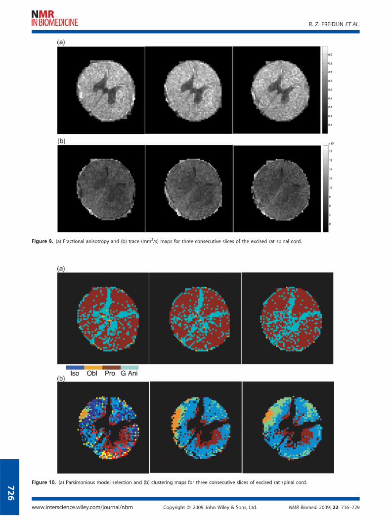
Excised rat spinal cord DTI experiment

Figure 9a and b shows the orientationally invariant FA and Tr maps for three consecutive slices. By examining these maps, we can only distinguish white from gray matter groups, although the white matter itself consists of several different fiber compartments.

& Sons, Ltd. www.interscience.wiley.com/journal/nbm

23

R. Z. FREIDLIN ET AL.

Figure 6. Performance comparison for the oblate and prolate regions at (a) SNR ¼ 33; (b) SNR ¼ 25; and (c) SNR ¼ 20, where ‘Lower’ FAs are represented by the darker bar and ‘Higher’ FAs by the lighter bar. The true positive counts are calculated within the areas of corresponding clusters, while the false positive counts are obtained from the outside regions.

724

Parsimonious model selection consistently segmented the prolate regions in white matter (Fig. 10a). However, the parsimonious model map does not reveal different fiber patterns within white matter. The multivariate hypothesis testing base-d-clustering algorithm identified a number of distinct prolate regions (Fig. 10b). Furthermore, by analogy with the results in the Synthetic

Phantoms with Partial Volumes subsection, we generated a difference map between the parsimonious model map of prolate voxels only and the sum of all prolate clusters. These results are shown in Fig. 11c, where voxels depicted in green correspond to reclassified as prolate, and voxels depicted in orange correspond to the edges of white matter, thus, most likely, containing partial volumes.

Excised pig spinal cord DTI experiment

Figure 12a and b shows the orientationally invariant FA and Tr maps. As in the excised rat spinal cord experiment (above), the prolate model (in Fig. 12c) depicted in red) was consistently selected as a white matter region. Figure 12d shows the results of

www.interscience.wiley.com/journal/nbm Copyright © 200

the unsupervised clustering algorithm (colors represent different clusters within white matter), which reveals similarities with the known histology of the spinal cord (Fig. 13) (39).

DISCUSSION

The aim of this work is to investigate the feasibility of using a multivariate hypothesis testing framework for automated tissue clustering and classification. As long as the conditions for normally distributed residuals and

uniform variances within each voxel of a diffusion-weighted image are met, this algorithm can be robustly used for clustering and classifying high resolution data obtained from tissue. To prevent clustering voxels in areas with inhomogeneous variance, which is observed in voxels with different degrees of diffusion anisotropy (35), we perform parsimonious model selection procedures prior to the clustering algorithm. Such model pre-selection ensures that the seed voxels for launching clusters are already described by the same diffusion models, thus improving the accuracy of the results.

9 John Wiley & Sons, Ltd. NMR Biomed. 2009; 22: 716–729

TISSUE CLUSTERING AND CLASSIFICATION OF DTI DATA

Figure 7. The phantom with partial volumes at SNR ¼ 30: (a) FA; (b) Tr (mm2/s); and (c) parsimonious model selection maps; (d) the identified clusters (colors depict different clusters and are not related to colors in the parsimonious model map). This figure is available in color online at www.interscience.wiley.com/journal/nbm

Monte Carlo simulations (not presented in this work) have shown that the clustering algorithm is more sensitive to trace differences, DTr, between regions having lower FAs (less than 0.7) than higher FAs. It was determined that for SNR ¼ 33 and FA < 0.7,

Figure 8. The phantom with partial volumes at SNR ¼ 30: (a) voxels identifiedall prolate clusters obtained from the clustering algorithm; (c) the difference bewith partial volumes are shown in green and orange colors, respectively. Thisnbm

NMR Biomed. 2009; 22: 716–729 Copyright © 2009 John Wiley

the clusters were correctly separated for DTr > 300 x 10 -6 mm2/s and the difference between FAs, DFA > 0.5. Otherwise, it was sufficient to set DTr ¼ 200 x 10 -6 mm2/s and DFA > 0.5. For the lower SNRs, clustering results showed an average of 95% success

by the parsimonious model selection algorithm as prolate; (b) the union of tween (a) and (b) maps, where correctly reclassified and unclustered voxels figure is available in color online at www.interscience.wiley.com/journal/

& Sons, Ltd. www.interscience.wiley.com/journal/nbm

725

R. Z. FREIDLIN ET AL.

Figure 9. (a) Fractional anisotropy and (b) trace (mm2/s) maps for three consecutive slices of the excised rat spinal cord.

Figure 10. (a) Parsimonious model selection and (b) clustering maps for three consecutive slices of excised rat spinal cord.

www.interscience.wiley.com/journal/nbm Copyright © 2009 John Wiley & Sons, Ltd. NMR Biomed. 2009; 22: 716–729

726

TISSUE CLUSTERING AND CLASSIFICATION OF DTI DATA

Figure 11. Excised rat spinal cord: (a) voxels identified by the parsimonious model selection algorithm as prolate; (b) the union of all prolate clusters obtained with the clustering algorithm; (c) the difference between (a) and (b) maps.

at DTr > 400 x 10- 6 mm2/s for FAs > 0.65 and DFA ¼ 0.1. We also noticed that at FAs greater than 0.9, some voxels were left unclustered. This could be attributed to forcing negative eigenvalues (l3), observed at the high FAs, to be positive. Voxels in the oblate and prolate regions, which were misclassified as general anisotropic by the parsimonious model selection algorithm, were correctly reclassified as oblate/prolate with at least 98% success at SNRs greater than 20.

Figure 12. Excised pig spinal cord: (a) the fractional anisotropy and (b) traceorange–oblate, red–prolate, and turquoise–general anisotropic models); (d) clusters).

NMR Biomed. 2009; 22: 716–729 Copyright © 2009 John Wiley

It was also observed (results are not presented in this work) that at the significance levels below 5% there was an increase in accepting false null hypotheses due to voxels with partial volumes. In such cases, overall performance of the proposed clustering algorithm at SNR : 20 and FAs greater than 0.6 was decreased on average by 5%. However, results were consistent for a range of significance levels in the regions without voxels containing partial volumes (SNR : 20 and FA : 0.6). Furthermore,

(mm2/s) maps; (c) color-coded parsimonious model map (blue–isotropic, identified clusters for the prolate model regions (colors depict different

& Sons, Ltd. www.interscience.wiley.com/journal/nbm

727

R. Z. FREIDLIN ET AL.

Figure 13. Schematic diagram of important sensory pathways in rat spinal cord white matter: (1) vestibulospinal; (2) anterior corticospinal; (3) spinothalamic; (4) lateral corticospianal; (5) spinocerebellar; (6) reticulosp­inal; (7) fasciculus cuneatus; (8) fasciculus gracilis; and (9) gray matter.

728

at the SNRs < 20 and FAs < 0.6 performance of the proposed method on average was reduced by 50% for fewer than 21 DWIs and 20% for more than 21 directions. From Monte Carlo simulations, we have determined that the

accuracy and the sensitivity of the multivariate hypothesis testing to the degrees of prolateness/oblateness, as well as, spatial orientation are closely related to the performance of the diffusion tensor estimation. Thus, for a nonlinear least-square minimization method, proposed by Koay et al., at SNRs < 20 it is advisable to acquire a minimum number of 25 DWIs. For example, at SNRs < 20, in order to differentiate between the regions with DTr ¼ 200 x 10 -6 mm2/s and DFA ¼ 0.05, the number of DWIs had to be set to 33. However, the proposed clustering method performed with 98% accuracy when the regions had DTr ¼ 400 x 10 -6 mm2/s and DFA ¼ 0.1 for FA : 0.6 with only 12 diffusion encoding directions. In general, the multivariate hypothesis testing framework for

tissue clustering is fast and simple to implement. Due to its unsupervised nature, the results from such tests are fully reproducible for high-resolution data, i.e. low number of voxels with partial volumes, and provide quantitative information about underlying tissue structures. In addition, we have shown that the clusters with similar FAs and/or Trs might have different underlying structures. This implies that clustering methods based upon thresholding criteria may incorrectly classify and cluster tissues having different properties. By looking at the entire tensor, we are able to discriminate between different tissue types more accurately. However, it is important to note that the voxels with partial volume (e.g. voxels that contain two fibers with different degrees of prolateness and/or diffusion orientations) may be assigned to different clusters depending on the starting seed region. This inconsistency can be resolved by identifying the most probable seed regions prior to clustering or by explicitly including partial-volume models in the parsimonious model selection hierarchy. Furthermore, when determining the number of voxels in the seed region, it is important to consider the resolution of DTI data and the size of the underlying structure of interest. However, the seed region should contain at least three adjacent voxels. In addition, it was observed that at low SNRs or for 21 or fewer DWI acquisitions, which contribute to higher variability in the estimated diffusion parameters, the proposed clustering method performed on average 10% better for the

www.interscience.wiley.com/journal/nbm Copyright © 200

2 x 2 seed region than the larger regions. This is because as the number of voxels in the seed region grows, so does the net variability within the sample. This causes the F-test to be more forgiving. The voxel-by-voxel approach allows us to cluster regions which

are not connected to each other without invoking a pre-defined number of clusters. However, segmented regions tend to be noisier than the results of segmentation based on such techniques as level sets and dissimilarity measures. Since, in its current implementation the proposed multivariate

hypothesis testing algorithm is very sensitive to changes in diffusion directionality, it is suitable for clustering tissues with well-defined orientations. Work is underway to extend this approach to identifying clusters, rather than individual tensors, with similar degrees of oblateness/prolateness, yet different spatial orientations.

CONCLUSIONS

The ability to identify different tissue types within white or gray matter has the potential to improve the diagnosis of a variety of neurological disorders, and to assess changes occurring in normal and abnormal development. However, before using the multi­variate hypothesis testing framework, it is important to ensure normality and equality of the variances for the diffusion tensor estimator and functions derived from it. We satisfy these conditions by applying the nonlinear least-squares estimator and the parsimonious model selection procedures prior to clustering. In addition, the parsimonious model selection framework improves automatic ROI delineation and classification of different tissue types by providing additional information about the underlying diffusion model. Given the simplicity and speed of the proposed F-test

clustering framework, it is feasible to process large high-resolution microscopic DTI datasets. Encouraging results from phantom simulations increase our confidence in clustering ex vivo tissue specimens where background noise is the primary artifact. However, in clinical applications other systematic artifacts should be reduced or carefully considered prior to applying multivariate hypothesis testing for clustering.

Acknowledgements

RZF thanks Kenneth Kempner for his support and encourage­ment. The authors would like to thank Dr Carlo Pierpaoli and Dr Uri Nevo for helpful discussions and Liz Salak for editing this paper. This research was supported by the Intramural Research Program of the National Institute of Child Health and Develop­ment (NICHD) and the Center for Information Technology (CIT), National Institutes of Health, Bethesda, Maryland.

REFERENCES

1. Basser PJ, Mattiello J, LeBihan D. MR diffusion tensor spectroscopy and imaging. Biophys. J. 1994; 66(1): 259–267.

2. Beaulieu C, Allen PS. Determinants of anisotropic water diffusion in nerves. , Magn. Reson. Med. 1994; 31(4): 394–400.

3. Jones DK, Simmons A, Williams SC, Horsfield MA. Non-invasive assessment of axonal fiber connectivity in the human brain via diffusion tensor MRI. Magn. Reson. Med. 1999; 42(1): 37–41.

9 John Wiley & Sons, Ltd. NMR Biomed. 2009; 22: 716–729

TISSUE CLUSTERING AND CLASSIFICATION OF DTI DATA

4. Mori S, Crain BJ, Chacko VP, van Zijl. PC. Three-dimensional tracking of axonal projections in the brain by magnetic resonance imaging. Ann. Neurol. 1999; 45(2): 265–269.

5. Basser PJ, Pajevic S, Pierpaoli C, Duda J, Aldroubi A. In vivo fiber tractography using DT-MRI data. 2000; Magn. Reson. Med. 44(4): 625–632.

6. Tench CR, Morgan PS, Wilson M, Blumhardt LD. White matter mapping using diffusion tensor MRI. Magn. Reson. Med. 2002; 47(5): 967–972.

7. Hagmann P, Thiran J-P, Jonasson L, Vandergheynst P, Clarke S, Maeder P, Meuli R. DTI mapping of human brain connectivity: statistical fibre tracking and virtual dissection. Neuroimage 2003; 19(3): 545–554.

8. Van Der Vaart H. Some results on the probability distribution of the latent roots of a symmetric matrix of continuously distributed elements, and some applications to the theory of response surface estimation. Report issued by the Institute of Statistics, University of North Carolina. 1958.

9. Pierpaoli C, Basser PJ. Toward a quantitative assessment of diffusion anisotropy. Magn. Reson. Med. 1996; 36(6): 893–906.

10. Zhukov L, Museth K, Breen D, Whitaker R, Barr A. Level set modelling and segmentation of DT-MRI brain data. J. Electron. Imaging 2003; 12(1): 125–133.

11. Li W, Tian J, Li E, Dai J. Robust unsupervised segmentation of infarct lesion from diffusion tensor MR images using multiscale statistical classification and partial volume voxel reclassification. Neuroimage 2004; 23(4): 1507–1518.

12. Basser PJ, Mattiello J, LeBihan D. Estimation of the effective self-diffusion tensor from the NMR spin echo. J. Magn. Reson. B 1994; 103(3): 247–254.

13. Feddern C, Weickert J, Burgeth B. Level-set methods for tensor-valued images. In Proceedings of the 2nd IEEE Workshop Variational, Geometric and Level Set Methods in Computer Vision, 2003; 65–72.

14. Wiegell MR, Tuch DS, Larsson HBW, Wedeen VJ. Automatic segmenta­tion of thalamic nuclei from diffusion tensor magnetic resonance imaging. Neuroimage 2003; 19(2 Pt 1): 391–401.

15. Wang Z, Vemuri BC. Tensor field segmentation using region based active contour model. In Computer Vision – ECCV 2004, Pt 4, 2004; 304–315.

16. Wang Z, Vemuri BC. DTI segmentation using an information theoretic tensor dissimilarity measure. IEEE Trans. Med. Imaging 2005; 24(10): 1267–1277.

17. Rousson M, Lenglet C, Deriche R. Level set and region based surface propagation for diffusion tensor mri segmentation. In ECCV Work­shops CVAMIA and MMBIA, 2004; 123–134.

18. Lenglet C, Rousson M, Deriche R. Segmentation of 3D probability density fields by surface evolution: application to diffusion MRI. In Proc. Medical Image Computing and Computer-Assisted Intervention – MICCAI 2004, Pt 1, 2004; 18–25.

19. Lenglet C, Rousson M, Deriche R, Faugeras O, Lehericy S, Ugurbil K. A Riemannian approach to diffusion tensor images segmentation. Inf. Process. Med. Imaging 2005; 19: 591–602.

20. Jonasson L, Hagmann P, Pollo C, Bresson X, Richero Wilson C, Meuli R, Thiran J. A level set method for segmentation of the thalamus and its nuclei in DT-MRI. Signal Processing 2007; 87(2): 309–321.

21. Alexander DC, Gee JC, Bajcsy R. Similarity measures for matching diffusion tensor images. In Proc. British Machine Vision Conference (BMVC), 1993; 93–102.

NMR Biomed. 2009; 22: 716–729 Copyright © 2009 John Wiley

22. Wang Z, Vemuri B. An affine invariant tensor dissimilarity measure and its applications to tensor-valued image segmentation. In IEEE Com­puter Society Conference on Computer Vision and Pattern Recognition, CVPR, 2004; I-228–I-233.

23. Awate SP, Zhang H, Gee JC. A fuzzy, nonparametric segmentation framework for DTI and MRI analysis: with applications to DTI-tract extraction. IEEE Trans. Med. Imaging 2007; 26(11): 1525–1536.

24. Ziyan U, Tuch D, Westin C-F. Segmentation of thalamic nuclei from DTI using spectral clustering. Ninth Int. Conf. Med. Image Comput. Com-put. Assist. Interv. 2006; 9(Pt 2): 807–814.

25. Khurd P, Verma R, Davatzikos C. Kernel-based manifold learning for statistical analysis of diffusion tensor images. Inf. Process. Med. Imaging 2007; 20: 581–593.

26. Whitcher B, Wisco JJ, Hadjikhani N, Tuch DS. Statistical group com­parison of diffusion tensors via multivariate hypothesis testing. Magn. Reson. Med. 2007; 57(6): 1065–1074.

27. Snedecor GW, Cochran WG. Statistical Methods, 8th edn., Iowa State University Press, 1989.

28. Hext GR. The estimation of second-order tensors, with related tests and designs. Biometrika 1963; 50: 353–357.

29. Freidlin RZ, Assaf Y, Basser PJ. Multivariate hypothesis testing of DTI data for tissue clustering. In IEEE Int. Symp. Biomed. Imag.: Macro to Nano (ISBI), 2007, 12–15 April 2007; 776–779.

30. Freidlin RZ, Assaf Y, Basser PJ. Multivariate hypothesis testing for tissue clustering and classification: a DTI study of excised rat spinal cord. In Joint Annual Meeting ISMRM-ESMRMB, 2007; 625.

31. Freidlin RZ, Ozarslan E, Komlosh ME, Chang L-C, Koay CG, Jones DK, Basser PJ. Parsimonious model selection for tissue segmentation and classification applications: a study using simulated and experimental DTI data. IEEE Trans. Med. Imaging 2007; 26(11): 1576–1584.

32. Schwarz G. Estimating the dimension of the model. Ann. Stat. 1978; 6: 461–468.

33. Stejskal EO, Tanner JE. Spin diffusion measurements: spin echoes in the presence of a time-dependent field gradient. J. Chem. Phys. 1966; 42(1): 288–292.

34. Koay CG, Chang L-C, Carew JD, Pierpaoli C, Basser PJ. A unifying theoretical and algorithmic framework for least squares methods of estimation in diffusion tensor imaging. J. Magn. Reson. 2006; 182(1): 115–125.

35. Carew JD, Koay CG, Wahba G, Alexander AL, Meyerand ME, Basser PJ. The asymptotic behavior of the nonlinear estimators of the Diffusion Tensor and tensor-derived quantities with implications for group analysis. Technical Report, Department of Statistics, University of Wisconsin, 2006.

36. Pierpaoli C, Jezzard P, Basser PJ, Barnett A, Chiro GD. Diffusion tensor MR imaging of the human brain. Radiology 1996; 201(3): 637– 648.

37. Henkelman RM. Measurement of signal intensities in the presence of noise in MR images. Med. Phys. 1985; 12(2): 232–233.

38. Shepherd TM, Thelwall PE, Stanisz PE, Blackband SJ. Chemical fixation alters the water microenvironment in rat cortical brain slices— implications for MRI contrast mechanisms. Proc. Int. Soc. Magn. Reson. Med. 2005; 13: 619.

39. Tracey DJ, Ascending, descending pathways in the spinal cord. In The Rat Nervous System, Paxinos G (ed.). 2nd edn. Academic Press: San Diego, CA, 1995; 67–75.

729

& Sons, Ltd. www.interscience.wiley.com/journal/nbm