A Multiscale Pyramid Transform for Graph Signals Multiscale Pyramid Transform for Graph Signals ......

1

A Multiscale Pyramid Transform for Graph SignalsDavid I Shuman, Mohammad Javad Faraji, and Pierre Vandergheynst

Abstract—Multiscale transforms designed to process analogand discrete-time signals and images cannot be directly appliedto analyze high-dimensional data residing on the vertices of aweighted graph, as they do not capture the intrinsic geometricstructure of the underlying graph data domain. In this paper, weadapt the Laplacian pyramid transform for signals on Euclideandomains so that it can be used to analyze high-dimensional dataresiding on the vertices of a weighted graph. Our approach isto study existing methods and develop new methods for thefour fundamental operations of graph downsampling, graphreduction, and filtering and interpolation of signals on graphs.Equipped with appropriate notions of these operations, weleverage the basic multiscale constructs and intuitions fromclassical signal processing to generate a transform that yields botha multiresolution of graphs and an associated multiresolution ofa graph signal on the underlying sequence of graphs.

Index Terms—Signal processing on graphs, multiresolution,spectral graph theory, graph downsampling, Kron reduction,spectral sparsification, Laplacian pyramid, interpolation

I. INTRODUCTION

Multiscale transform methods can reveal structural informa-tion about signals, such as singularities or irregular structuralpatterns, at different resolution levels. At the same time,via coarse-to-fine analysis, they provide a way to reducethe complexity and dimensionality of many signal processingtasks, often resulting in fast algorithms. However, multiscaletransforms such as wavelets and filter banks designed toprocess analog and discrete-time signals and images cannotbe directly applied to analyze high-dimensional data residingon the vertices of a weighted graph, as they do not capturethe intrinsic geometric structure of the underlying graph datadomain (see [2] for an overview of the main challenges of thisemerging field of signal processing on graphs).

To address this issue, classical wavelets have recently beengeneralized to the graph setting in a number of different ways.Reference [2] contains a more thorough review of these graphwavelet constructions, which include, e.g., spatially-designedgraph wavelets [3], diffusion wavelets [4], spectral graphwavelets [5], lifting based wavelets [6], [7] critically sampled

This work was supported in part by FET-Open grant number 255931UNLocX.

Part of this work appeared in the master’s thesis [1] and waspresented at the Duke Workshop on Sensing and Analysis of High-Dimensional Data in July 2011. Slides and video are available athttp://sahd.pratt.duke.edu/2011 files/Videos and Slides.html

David I Shuman is with the Department of Mathematics, Statistics, andComputer Science, Macalester College, St. Paul, MN 55105, USA (email:[email protected]). Mohammad Javad Faraji is with the Compu-tational Neuroscience Laboratory (LCN), Ecole Polytechnique Federale deLausanne (EPFL), School of Computer and Communication Sciences andBrain Mind Institute, School of Life Sciences, CH-1015 Lausanne, Switzer-land (email: [email protected]). Pierre Vandergheynst is withthe Signal Processing Laboratory (LTS2), Ecole Polytechnique Federale deLausanne (EPFL), Institue of Electrical Engineering, CH-1015 Lausanne,Switzerland (email: [email protected]).

two-channel wavelet filter banks [8], critically-sampled splinewavelet filter banks [9], and multiscale wavelets on balancedtrees [10]. Multiresolutions of graphs also have a long historyin computational science problems including graph cluster-ing, numerical solvers for linear systems of equations (oftenarising from discretized differential equations), combinatorialoptimization problems, and computational geometry (see, e.g.,[11]-[14] and references therein). We discuss some of therelated work from these fields in Sections III-E and IV-E.

In this paper, we present a modular framework for adaptingBurt and Adelson’s Laplacian pyramid transform [15] to thegraph setting. Our main contributions are to (1) survey differ-ent methods for and desirable properties of the four fundamen-tal graph signal processing operations of graph downsampling,graph reduction, generalized filtering, and interpolation ofgraph signals (Sections III-V); (2) present new graph down-sampling and reduction methods, including downsamplingbased on the polarity of the largest Laplacian eigenvectorand Kron reduction followed by spectral sparsification; and(3) leverage these fundamental operations to construct a newmultiscale pyramid transform that yields both a multiresolutionof a graph and a multi-scale analysis of a signal residing onthat graph (Section VI). We also discuss some implementationapproximations and open issues in Section VII, as it isimportant that the computational complexity of the resultingmultiscale transform scales well with the number of verticesand edges in the underlying graph.

II. SPECTRAL GRAPH THEORY NOTATION

We consider connected, loopless (no edge connecting avertex to itself), undirected, weighted graphs. We representsuch a graph by the triplet G = {V, E , w}, where V is a set ofN vertices, E is a set of edges, and w : E → R+ is a weightfunction that assigns a non-negative weight to each edge. Anequivalent representation is G = {V, E ,W}, where W is aN ×N weighted adjacency matrix with nonnegative entries

Wij =

{w(e), if e ∈ E connects vertices i and j0, if no edge connects vertices i and j

.

In unweighted graphs, the entries of the adjacency matrix Ware ones and zeros, with a one corresponding to an edgebetween two vertices and a zero corresponding to no edge.The degree matrix D is a diagonal matrix with an ith diagonalelement Dii = di =

∑j∈NiWij , where Ni is the set of

vertex i’s neighbors in G. Its maximum element is dmax :=maxi∈V{di}. We denote the combinatorial graph Laplacianby L := D −W, the normalized graph Laplacian by L :=D−

12LD−

12 , and their respective eigenvalue and eigenvector

pairs by {(λ`,u`)}`=0,1,...,N−1 and {(λ`, u`)}`=0,1,...,N−1.Then U and U are the matrices whose columns are equal to the

2

eigenvectors of L and L, respectively. We assume without lossof generality that the eigenvalues are monotonically orderedso that 0 = λ0 < λ1 ≤ λ2 ≤ . . . ≤ λN−1, and we denotethe maximum eigenvalues and associated eigenvectors byλmax = λN−1 and umax = uN−1. The maximum eigenvalueλmax is said to be simple if λN−1 > λN−2.

III. GRAPH DOWNSAMPLING

Two key components of multiscale transforms for discrete-time signals are downsampling and upsampling.1 To down-sample a discrete-time sample by a factor of two, we removeevery other component of the signal. To extend many ideasfrom classical signal processing to the graph setting, we needto define a notion of downsampling for signals on graphs.Yet, it is not at all obvious what it means to remove everyother component of a signal f ∈ RN defined on the verticesof a graph. In this section, we outline desired properties of adownsampling operator for graphs, and then go on to suggestone particular downsampling method.

Let D : G = {V, E ,W} → 2V be a graph downsamplingoperator that maps a weighted, undirected graph to a subsetof vertices V1 to keep. The complement Vc1 := V\V1 ={v ∈ V : v /∈ V1} is the set of vertices that D removes fromV . Ideally, we would like the graph downsampling operator Dto have the following properties:(D1) It removes approximately half of the vertices of the

graph (or, equivalently, approximately half of the com-ponents of a signal on the vertices of the graph); i.e.,|D(G)| = |V1| ≈ |V|2 .

(D2) The set of removed vertices are not connected with edgesof high weight, and the set of kept vertices are notconnected with edges of high weight; i.e., if i, j ∈ V1,then Wij is low, and if i, j ∈ Vc1 , then Wij is low.

(D3) It has a computationally efficient implementation.

A. Vertex Selection Using the Largest Eigenvector of theGraph Laplacian

The method we suggest to use for graph downsampling isto select the vertices to keep based on the polarity of thecomponents of the largest eigenvector; namely, let

V1 = V+ := {i ∈ V : umax(i) ≥ 0} . (1)

We refer to this method as the largest eigenvector vertexselection method. A few remarks are in order regarding thischoice of downsampling operator. First, the polarity of thelargest eigenvector splits the graph into two components.In this paper, we choose to keep the vertices in V+, andeliminate the vertices in V− := {i ∈ V : umax(i) < 0}, butwe could just as easily do the reverse, or keep the verticesin Vbig := arg maxV1∈{V+,V−}|V1|, for example. Second, forsome graphs such as the complete graph, λmax is a repeatedeigenvalue, so the polarity of umax is not uniquely defined.In this case, we arbitrarily choose an eigenvector from the

1We focus here on downsampling, as we are only interested in upsamplingpreviously downsampled graphs. As long as we track the positions of theremoved components of the signal, it is straightforward to upsample byinserting zeros back into those components of the signal.

eigenspace. Third, we could just as easily base the vertexselection on the polarity of the normalized graph Laplacianeigenvector, umax associated with the largest eigenvalue,λmax. In some cases, such as the bipartite graphs discussednext, doing so yields exactly the same selection of verticesas downsampling based on the largest non-normalized graphLaplacian eigenvector; however, this is not true in general.

In the following sections, we motivate the use of the largesteigenvector of the graph Laplacian from two different perspec-tives - first from a more intuitive view as a generalization ofdownsampling techniques for special types of graphs, and thenfrom a more theoretical point of view by connecting the vertexselection problem to graph coloring, spectral clustering, andnodal domain theory.

B. Special Case: Bipartite Graphs

There is one situation in which there exists a fairly clearnotion of removing every other component of a graph signal– when the underlying graph is bipartite. A graph G ={V, E ,W} is bipartite if the set of vertices V can be par-titioned into two subsets V1 and Vc1 so that every edge e ∈ Elinks one vertex in V1 with one vertex in Vc1 . In this case, itis natural to downsample by keeping all of the vertices in oneof the subsets, and eliminating all of the vertices in the othersubset. In fact, as stated in the following theorem, the largesteigenvector downsampling method does precisely this in thecase of bipartite graphs.

Theorem 1 (Roth, 1989): For a connected, bipartite graphG = {V1∪Vc1 , E ,W}, the largest eigenvalues, λmax and λmax,of L and L, respectively, are simple, and λmax = 2. Moreover,the polarity of the components of the eigenvectors umax andumax associated with λmax and λmax both split V into thebipartition V1 and Vc1 . That is, for v = umax or v = umax,

v(i)v(j) > 0, if i, j ∈ V1 or i, j ∈ Vc1 , andv(i)v(j) < 0, if i ∈ V1, j ∈ Vc1 or i ∈ Vc1 , j ∈ V1. (2)

If, in addition, G is k-regular (di = k, ∀i ∈ V), then λmax =2k, and

umax = umax =

{1√N, if i ∈ V1

− 1√N, if i ∈ Vc1

.

The majority of the statements in Theorem 1 follow fromresults of Roth in [16], which are also presented in [17,Chapter 3.6].

The path, ring (with an even number of vertices), and finitegrid graphs, which are shown in Figure 1, are all examplesof bipartite graphs and all have simple largest graph Lapla-cian eigenvalues. Using the largest eigenvector downsamplingmethod leads to the elimination of every other vertex on thepath and ring graphs, and to the quincunx sampling pattern onthe finite grid graph (with or without boundary connections).

Trees (acyclic, connected graphs) are also bipartite. Anexample of a tree is shown in Figure 1(e). Fix an arbitraryvertex r to be the root of the tree T , let Y0

r be the singletonset containing the root, and then define the sets {Ytr}t=1,2,...

by Ytr := {i ∈ V : i is t hops from the root vertex r in T }.Then the polarity of the components of largest eigenvector

3

(a) (b)

(c) (d)

(e)

Fig. 1. Examples of partitioning structured graphs into two sets (red and blue)according to the polarity of the largest eigenvector of the graph Laplacian. Forthe path graph in (a) and the ring graph in (b), the method selects every othervertex like classical downsampling of discrete-time signals. For the finite gridgraphs with the ends unconnected (c) and connected (d), the method resultsin the quincunx sampling pattern. For a tree graph in (e), the method groupsthe vertices at every other depth of the tree.

of the graph Laplacian splits the vertices of the tree into twosets according to the parity of the depths of the tree. That is,if we let Yevenr := ∪t=0,2,...Ytr and Yoddr := ∪t=1,3,...Ytr, thenYevenr = V+ and Yoddr = V−, or vice versa.

In related work, [18] and [19] suggest to downsamplebipartite graphs by keeping all of the vertices in one subsetof the bipartition, and [20] suggests to downsample trees bykeeping vertices at every other depth of the tree. Therefore,the largest eigenvector downsampling method can be seen asa generalization of those approaches.

C. Connections with Graph Coloring and Spectral Clustering

A graph G = {V, E ,W} is k-colorable if there exists apartition of V into subsets V1,V2, . . . ,Vk such that if verticesi, j ∈ V are connected by an edge in E , then i and j are indifferent subsets in the partition. The chromatic number χ ofa graph G is the smallest k such that G is k-colorable. Thus,the chromatic number of a graph is equal to 2 if and only ifthe graph is bipartite.

As we have seen with the examples in the previous section,when a graph is bipartite, it is easy to decide how to split itinto two sets for downsampling. When the chromatic numberof a graph is greater than two, however, we are interested infinding an approximate coloring [21]; that is, a partition thathas as few edges as possible that connect vertices in the same

subset.2 As noted by [21], the approximate coloring problemis in some sense dual to the problem of spectral clustering(see, e.g. [22] and references therein).

Aspvall and Gilbert [21] suggest to construct an approx-imate 2-coloring of an unweighted graph according to thepolarity of the eigenvector associated with the most negativeeigenvalue of the adjacency matrix. For regular graphs, theeigenvector associated with the most negative eigenvalue of theadjacency matrix is the same as the largest graph Laplacianeigenvector, and so the method of [21] is equivalent to thelargest Laplacian eigenvector method for that special case.

D. Connections with Nodal Domain Theory

A positive (negative) strong nodal domain of f on G is amaximally connected subgraph such that f(i) > 0 (f(i) < 0)for all vertices i in the subgraph [17, Chapter 3]. A positive(negative) weak nodal domain of f on G is a maximallyconnected subgraph such that f(i) ≥ 0 (f(i) ≤ 0) for allvertices i in the subgraph, with f(i) 6= 0 for at least onevertex i in the subgraph.

A graph downsampling can be viewed as an assignmentof positive and negative signs to vertices, with positive signsassigned to the vertices that we keep, and negative signs tothe vertices that we eliminate. The goal of having few edgeswithin either the removed set or the kept set is closely relatedto the problem of maximizing the number of nodal domainsof the downsampling. This is because maximizing the numberof nodal domains leads to nodal domains with fewer vertices,which results in fewer edges connecting vertices within theremoved and kept sets.

Next, we briefly mention some general bounds on thenumber of nodal domains of eigenvectors of graph Laplacians:

(ND1) u` has at most ` weak nodal domains and `+s−1 strongnodal domains, where s is the multiplicity of λ` [23], [17,Theorem 3.1].

(ND2) The largest eigenvector umax has N strong and weaknodal domains if and only if G is bipartite. Moreover, ifHis an induced bipartite subgraph of G with the maximumnumber of vertices, then the number of vertices in H isan upper bound on the number of strong nodal domainsof any eigenvector of a generalized Laplacian of G [17,Theorem 3.27].

(ND3) If λ` is simple and u`(i) 6= 0, ∀i ∈ V , the number ofnodal domains of u` is greater than or equal to ` − r,where r is the number of edges that need to be removedfrom the graph in order to turn it into a tree3[24].

Note that while both the lower and upper bounds onthe number of nodal domains of the eigenvectors of graphLaplacians are monotonic in the index of the eigenvalue, theactual number of nodal domains is not always monotonic in theindex of the eigenvalue (see, e.g., [25, Figure 1] for an examplewhere they are not monotonic). Therefore, for arbitrary graphs,

2In other contexts, the term approximate coloring is also used in referenceto finding a proper k-coloring of a graph in polynomial time, such that k isas close as possible to the chromatic number of the graph.

3Berkolaiko proves this theorem for Schrodinger operators, which encom-pass generalized Laplacians of unweighted graphs.

4

it is not guaranteed that the largest eigenvector of the graphLaplacian has more nodal domains than the other eigenvectors.For specific graphs such as bipartite graphs, however, this isguaranteed to be the case, as can be seen from the abovebounds and Theorem 1. Finally, in the case of repeated graphLaplacian eigenvalues, [17, Chapter 5] presents a hillclimbingalgorithm to search for an associated eigenvector with a largenumber of nodal domains.

E. Alternative Graph Downsampling Methods

We briefly mention some alternative graph downsam-pling/partitioning methods:

1) As mentioned above, [21] partitions the graph based onthe polarity of the eigenvector associated with the mostnegative eigenvalue of the adjacency matrix.

2) We can do a k-means clustering on umax with k = 2to separate the sets. A closely related alternative is toset a non-zero threshold in (1). A flexible choice of thethreshold can ensure that |V1| ≈ N

2 .3) In [8], Narang and Ortega downsample based on the

solution to the weighted max-cut problem:

arg maxV1

{cut(V1,Vc1)

}= arg max

V1

{∑i∈V1

∑i′∈Vc1

Wii′

}.

This problem is NP-hard, so approximations must beused for large graphs.

4) Barnard and Simon [26] choose V1 to be a maximalindependent set (no edge connects two vertices in V1

and every vertex in Vc1 is connected to some vertex inV1). Maximal independent sets are not unique, but canbe found via efficient greedy algorithms.

5) Ron et al. propose the SelectCoarseNodes algorithm[13, Algorithm 2], which leverages an algebraic distancemeasure to greedily select those nodes which have largefuture volume, roughly corresponding to those nodesstrongly connected to vertices in the eliminated set.

Additionally, there are a number of graph coarsening methodswhere the reduced set of vertices is not necessarily a subset ofthe original set of vertices. We discuss those further in SectionIV-E.

IV. GRAPH REDUCTION

So we now have a way to downsample a graph to a subsetof the vertices. However, in order to implement any typeof multiscale transform that will require filtering operationsdefined on the subset of selected vertices, we still need todefine a method to reduce the graph Laplacian on the originalset of vertices to a new graph Laplacian on the subset ofselected vertices. We refer to this process as graph reduction.For the purpose of mutliscale transforms, we would ideallylike the graph reduction method to have some or all of theproperties listed below. Note that the following represents oneexample of desiderata and is neither exhaustive nor definitive.

(GR1) The reduction is in fact a graph Laplacian (i.e., a symmet-ric matrix with row sums equal to zero and nonpositiveoff-diagonal elements).

(GR2) It preserves connectivity. That is, if the original graph isconnected, then the reduced graph is also connected.

(GR3) The spectrum of the reduced graph Laplacian is repre-sentative of and contained in the spectrum of the originalgraph Laplacian.

(GR4) It preserves structural properties (e.g., if the originalgraph is a tree or bipartite, the reduced graph is accord-ingly a tree or bipartite).

(GR5) Edges in the original graph that connect vertices in thereduced vertex set are preserved in the reduced graph.

(GR6) It is invertible or partially invertible with some sideinformation; i.e., from the reduced graph Laplacian andpossibly some other stored information, we can recoverthe original graph Laplacian.

(GR7) It is computationally efficient to implement.(GR8) It preserves graph sparsity. That is, the ratio of the

number of edges over potential edges(

|E|N(N−1)/2

)does

not increase too much from the original graph to thereduced graph. In addition to preserving computationalbenefits associated with sparse matrix-vector multiplica-tion, keeping this ratio low ensures that the reduced graphalso captures local connectivity information and not justglobal information.

(GR9) There is some meaningful correspondence between theeigenvectors of the reduced graph Laplacian and the orig-inal graph Laplacian; for example, when restricted to thekept set of vertices, the lowest (smoothest) eigenvectorsof the original Laplacian are similar to or the same as theeigenvectors of the reduced Laplacian.

In the following, we discuss in detail one particular choiceof graph reduction that satisfies some, but not all, of theseproperties. In Section IV-E, we briefly mention a few othergraph reduction methods.

A. Kron Reduction

The starting point for the graph reduction method we con-sider here is Kron reduction (see [27] and references therein).We start with a weighted graph G = {V, E ,W}, its associatedgraph Laplacian L, and a subset V1 ( V of vertices (the setselected by downsampling, for example) on which we want toform a reduced graph.4 The Kron reduction of L is the Schurcomplement [28] of L relative to LVc1 ,Vc1 ; that is, the Kronreduction of L is given by

K (L,V1) := LV1,V1 − LV1,Vc1L−1Vc1 ,Vc1

LVc1 ,V1 , (3)

where LA,B denotes the |A| × |B| submatrix consistingof all entries of L whose row index is in A and whosecolumn index is in B. We can also uniquely associatewith LKron−reduced = K (L,V1) a reduced weighted graphGKron−reduced =

{V1, EKron−reduced,WKron−reduced} by

letting

WKron−reducedij =

{−LKron−reducedij if i 6= j,0 o.w.

, (4)

4We assume |V1| ≥ 2.

5

and taking EKron−reduced to be the set of edges with non-zeroweights in (4).5 An example of Kron reduction is shown inFigure 2.

2

2

111

119

119

29

1627

23

94

32

158

4 2

10

2

4

4

196

6

6

6 6

6

6

6

2 2

6 1

Kron

Fig. 2. An example of Kron reduction. The vertices in V1 are in red, andthose in V c

1 are in blue.

B. Properties of Kron Reduction

For a complete survey of the topological, algebraic, andspectral properties of the Kron reduction process, see [27]. Inthe next theorem, we summarize the results of [27] that are ofmost interest with regards to multiscale transforms.

Theorem 2 (Dorfler and Bullo, 2013): Let L be a graphLaplacian of an undirected weighted graph G on the vertexset V , V1 ( V be a subset of vertices with |V1| ≥ 2,LKron−reduced = K (L,V1) be the Kron-reduced graph Lapla-cian defined in (3), and GKron−reduced be the associated Kron-reduced graph. Then(K1) The Kron-reduced graph Laplacian in (3) is well-defined(K2) LKron−reduced is indeed a graph Laplacian(K3) If the original graph G is connected (i.e., λ1(L) > 0),

then the Kron-reduced graph GKron−reduced is alsoconnected (i.e., λ1(LKron−reduced) > 0)

(K4) If the original graph G is loopless, then the Kron-reducedgraph GKron−reduced is also loopless6

(K5) Two vertices i, j ∈ V1 are connected by an edge if andonly if there is a path between them in G whose verticesall belong to {i, j} ∪ Vc1

(K6) Spectral interlacing: for all ` ∈ {0, 1, . . . , |V1| − 1},

λ`(L) ≤ λ`(LKron−reduced) ≤ λ`+|V|−|V1|(L). (5)

In particular, (5) and property (K4) above imply

0 = λmin(L) = λmin(LKron−reduced)≤ λmax(LKron−reduced) ≤ λmax(L) (6)

(K7) Monotonic increase of weights: for all i, j ∈ V1,WKron−reducedij ≥Wij

(K8) Resistance distance [29] preservation: for all i, j ∈ V1,

dRG (i, j) := (δi − δj)TL†(δi − δj)= (δi − δj)T(LKron−reduced)†(δi − δj),

where L† is the pseudoinverse of L and δi is theKronecker delta (equal to 1 at vertex i and 0 at all othervertices)

5In (4), we still index the new weights by the same vertex indices i and j.In practice, the vertices i and j will receive new ordinal indices between 1and NKron−reduced = |V1|, the number of vertices in the reduced graph.

6While [27] considers the more general case of loopy Laplacians, the graphswe are interested in are all loopless; that is, there are no self-loops connectinga vertex to itself, and therefore Lnn =

∑i∈V,i 6=nWni.

(a) (b)

32

31

21

41

127

(c) (d)

61 2

1

31

31

31

51

(e)

Fig. 3. Kron reductions of the graphs of Figure 1, with the blue verticeseliminated. If the weights of all of the edges in the original path and ringgraphs are equal to 1, then the weights of all of the edges in the Kron-reducedgraphs in (a) and (b) are equal to 1

2. For the Kron reduction of the finite grid

graph with the ends connected (d), the weights of the blue edges are equal to12

and the weights of the black edges are equal to 14

. The weights of Kronreductions of the finite grid graph with the ends unconnected (c) and the treegraph (e) are shown by color next to their respective Kron reductions.

C. Special Cases

As in Section III-B for the vertex selection process, weanalyze the effect of Kron reduction on some special classesof graphs in order to (i) provide further intuition behind thegraph reduction process; (ii) show that Kron reduction is ageneralization of previously suggested techniques for reducinggraphs belonging to these special classes; and (iii) highlightboth the strengths and weaknesses of this choice of graphreduction.

1) Paths: The class of path graphs is closed under thesequential operations of largest eigenvector vertex selectionand Kron reduction. That is, if we start with a path graph GPwith N vertices, and select a subset V1 according the polarityof the largest eigenvector of the graph Laplacian of GP , thenthe graph associated with K (GP ,V1) is also a path graph. Ifthe weights of the edges of the original graph are all equal to1, the weights of the edges of the Kron-reduced graph are allequal to 1

2 . The Kron reduction of the graph shown in Figure1(a) is shown in Figure 3(a).

2) Rings: The Kron reduction of the ring graph shown inFigure 1(b) is shown in Figure 3(b). It is a ring graph withhalf the number of vertices, and the weights of the edges arealso halved in the Kron reduction process.

3) Finite Grids: The Kron reductions of the finite gridgraphs shown in Figure 1(c,d) are shown in Figure 3(c,d). Ifwe rotate Figure 3(c) clockwise by ninety degrees, we see thatit is a subgraph of the 8-connected grid. We do not consider

6

graphs with infinite vertices here, but the combined effect ofthe largest eigenvector vertex selection and Kron reductionoperations is to map an infinite (or very large) 4-connectedgrid to an 8-connected grid.

4) Trees: The Kron reduction of the tree shown in Figure1(e) is shown in Figure 3(e). Note that the Kron reduction ofa tree is not a tree because siblings in the original graph areconnected in the Kron-reduced graph. However, it does have aparticular structure, which is a union of complete subgraphs.For every node i in the reduced graph, and each one of thatnode’s children j in the original graph, there is a completesubgraph in the reduced graph that includes i and all of thechildren of j (i.e., the grandchildren of i through j). If theweights of the edges in the original graph are equal to one,then the weights in each of the complete subgraphs are equalto one over the number of vertices in the complete subgraph.

This class of graphs highlights two of the main weaknessesof the Kron reduction: (i) it does not always preserve regularstructural properties of the graph; and (ii) it does not alwayspreserve the sparsity of the graph. We discuss a sparsity-enhancing modification in Section IV-D.

5) k-Regular Bipartite Graphs: In [18], Narang and Ortegaconsider connected and unweighted k-RBGs.7 They downsam-ple by keeping one subset of the bipartition, and they constructa new graph on the downsampled vertices V1 by linkingvertices in the reduced graph with an edge whose weight isequal to the number of their common neighbors in the originalgraph. If the vertices of the original graph are rearranged sothat all the vertices in V1 have smaller indices than all thevertices in Vc1 , the adjacency and Laplacian matrices of theoriginal graph can be represented as:

W =

[0 W1

WT1 0

]and L =

[kIN

2−W1

−WT1 kIN

2

]. (7)

Then for all i, j ∈ V1 (with i 6= j), the (i, j)th entry of theadjacency matrix of the reduced graph is given by

W kRBG−reducedij (V1) = (W1W

T

1 )ij . (8)

They also show that

LkRBG−reduced(V1) = k2IN2−W1W

T

1. (9)

Now we examine the Kron reduction of k-RBGs. The Kron-reduced Laplacian is given by:

LKron−reduced(V1) = LV1,V1 − LV1,Vc1L−1Vc1 ,Vc1

LVc1 ,V1= kIN

2− (−W1)(kIN

2)−1(−WT

1)

= kIN2− 1

kW1W

T

1,

which is a constant factor 1k times the reduced Laplacian (9)

of [18]. So, up to a constant factor, the Kron reduction is ageneralization of the graph reduction method presented in [18]for the special case of regular bipartite graphs.

7Although [18] considers unweighted k-RBGs, the following statementsalso apply to weighted k-RBGs if we extend the definition of the reducedadjacency matrix (8) to weighted graphs.

Algorithm 1 Spectral Sparsification [30]Inputs: G = {V, E ,W}, QOutput: W′

1: Initialize W′ = 02: for q = 1, 2, . . . , Q do3: Choose a random edge e = (i, j) of E according to the

probability distribution

pe =dRG (i, j)Wij∑

e=(m,n)∈EdRG (m,n)Wmn

4: W ′ij = W ′ij +Wij

Qpe5: end for

(a) (b) (c)

(d) (e) (f)

Fig. 4. Incorporation of a spectral sparsification step into the graph reduction.(a)-(c) Repeated largest eigenvector downsampling and Kron reduction of asensor network graph. (d)-(f) The same process with the spectral sparsificationof [30] used immediately after each Kron reduction.

D. Graph Sparsification

As a consequence of property (K5), repeated Kron reductionoften leads to denser and denser graphs. We have already seenthis loss of sparsity in Section IV-C4, and this phenomenonis even more evident in larger, less regular graphs. In additionto computational drawbacks, the loss of sparsity can be im-portant, because if the reduced graphs become too dense, theymay not effectively capture the local connectivity informationthat is important for processing signals on the graph. There-fore, in many situations, it is advantageous to perform graphsparsification immediately after the Kron reduction as part ofthe overall graph reduction phase.

There are numerous ways to perform graph sparsification.In this paper, we use a straightforward spectral sparsificationalgorithm of Spielman and Strivastava [30], which is describedin Algorithm 1. This sparsification method pairs nicely withthe Kron reduction, because [30] shows that for large graphsand an appropriate choice of the number of samples Q, thegraph Laplacian spectrum and resistance distances betweenvertices are approximately preserved with high probability.In Figure 4, we show an example of repeated downsamplingfollowed by Kron reduction and spectral sparsification.

E. Alternative Graph Reduction Methods

First, we mention some alternative graph reduction methods:

7

1) In [8], Narang and Ortega define a reduced graph viathe weighted adjacency matrix by taking W(j+1) =([W(j)]2

)V1,V1

. Here, [W(j)]2 represents the 2-hop ad-jacency matrix of the original graph. The reduced Lapla-cian can then be defined as L(j+1) = D(j+1)−W(j+1),where D(j+1) is computed from W(j+1). However,there are a number of undesirable properties of thisreduction method. First, and perhaps foremost, the re-duction method does not always preserve connectivity.Second, self-loops are introduced at every vertex in thereduced graph. Third, vertices in the selected subsetthat are connected by an edge in the original graphmay not share an edge in the reduced graph. Fourth,the spectrum of the reduced graph Laplacian is notnecessarily contained in the spectrum of the originalgraph Laplacian.

2) Ron et al. [13] assign a fraction Pij of each vertexi in the original graph to each vertex j ∈ V1 in thereduced graph that is close to i in the original graph (interms of an algebraic distance). The assignment satisfies∑j∈V1 Pij = 1 for all i ∈ V and Pjj = 1 for all j ∈ V1,

and for each eliminated vertex i ∈ Vc1 , an upper limitis placed on the number of vertices j ∈ V1 that havePij > 0. Then for all j, j′ ∈ V1,

W reducedjj′ :=

∑m,n∈V,m 6=n

PmjPnj′Wmn.

Next, we mention some graph coarsening (also called coarse-graining) methods that combine graph downsampling andreduction into a single operation by forming aggregate nodes ateach resolution, rather than keeping a strict subset of originalvertices. The basic approach of these methods is to partitionthe original set of vertices into clusters, represent each clusterof vertices in the original graph with a single vertex in thereduced graph, and then use the original graph to form edgesand weights that connect the representative vertices in thereduced graph. Some examples include:

1) Lafon and Lee [31] cluster based on diffusion distancesand form new edge weights based on random walktransition probabilities.

2) The Lean Algebraic Multigrid (LAMG) method of [32]builds each coarser Laplacian by selecting seed nodes,assigning each non-seed node to be aggregated withexactly one seed node, and setting the weights betweentwo new seed nodes j and j′ to be

W reducedjj′ :=

∑i∈Vj

∑i′∈Vj′

Wii′ ,

where Vj and Vj′ are the sets of vertices that havebeen aggregated with seeds j and j′, respectively. Theseed assignments are based on an affinity measure thatapproximates short time diffusion distances, rather thanthe algebraic distances used in [13].

3) Multilevel clustering algorithms such as those presentedin [33], [34] often use greedy coarsening algorithms suchas heavy edge matching or max-cut coarsening (see [33,Section 3] and [34, Section 5.1] for details).

For more thorough reviews of the graph partitioning andcoarsening literature, see, e.g., [11], [13], [35].

To summarize, given a graph G and a desired number ofresolution levels, in order to generate a multiresolution ofgraphs, we only need to choose a downsampling operator anda graph reduction method. In the remainder of the paper, weuse the largest eigenvector downsampling operator and theKron reduction with the extra sparsification step to generategraph multiresolutions such as the three level one shown inFigure 4(d)-(f). Note that graph multiresolutions generated inthis fashion are completely independent of any signals residingon the graph.

V. FILTERING AND INTERPOLATION OF GRAPH SIGNALS

Equipped with a graph multiresolution, we now proceed toanalyze signals residing on the finest graph in the multiresolu-tion. The two key graph signal processing components we usein the proposed transform are a generalized filtering operatorand an interpolation operator for signals on graphs. Filtersare commonly used in classical signal processing analysis toseparate a signal into different frequency bands. In this section,we review how to extend the notion of filtering to graphsignals. We focus on graph spectral filtering, which leveragesthe eigenvalues and eigenvectors of Laplacian operators fromspectral graph theory [36] to capture the geometric structure ofthe underlying graph data domain. We then discuss differentmethods to interpolate from a signal residing on a coarsergraph to a signal residing on a finer graph whose vertices area superset of those in the coarser graph.

A. Graph Spectral FilteringA graph signal is a function f : V → R that associates a

real value to each vertex of the graph. Equivalently, we canview a graph signal as a vector f ∈ RN .

In frequency filtering, we represent signals as linear com-binations of a set of signals and amplify or attenuate thecontributions of different components. In classical signal pro-cessing, the set of component signals are usually the complexexponentials, which carry a notion of frequency and give riseto the Fourier transform. In graph signal processing, it is mostcommon to choose the graph Fourier expansion basis to bethe eigenvectors of the combinatorial or normalized graphLaplacian operators. This is because the spectra of these graphLaplacians also carry a notion of frequency (see, e.g., [2,Figure 3]), and their eigenvectors are the graph analogs tothe complex exponentials, which are the eigenfunctions of theclassical Laplacian operator.

More precisely, the graph Fourier transform with the com-binatorial graph Laplacian eigenvectors as a basis is

f(λ`) := 〈f ,u`〉 =

N∑i=1

f(i)u∗` (i), (10)

and a graph spectral filter, which we also refer to as a kernel, isa real-valued mapping h(·) on the spectrum of graph Laplacianeigenvalues. Just as in classical signal processing, the effectof the filter is multiplication in the Fourier domain:

fout(λ`) = fin(λ`)h(λ`), (11)

8

or, equivalently, taking an inverse graph Fourier transform,

fout(i) =

N−1∑`=0

fin(λ`)h(λ`)u`(i). (12)

We can also write the filter in matrix form as fout = Hfin,where H is a matrix function [37]

H = h(L) = U[h(Λ)]U∗, (13)

where h(Λ) is a diagonal matrix with the elements of thediagonal equal to {h(λ`)}`=0,1,...,N−1. We can also use thenormalized graph Laplacian eigenvectors as the graph Fourierbasis, and simply replace L, λ`, and u` by L, λ`, and u` in(10)-(13). A discussion of the benefits and drawbacks of eachof these choices for the graph Fourier basis is included in [2].

B. Alternative Filtering Methods for Graph SignalsWe briefly mention two alternative graph filtering methods:1) We can filter a graph signal directly in the vertex

domain by writing the output at a given vertex i as alinear combination of the input signal components ina neighborhood of i. Graph spectral filtering with anorder K polynomial kernel can be viewed as filteringin the vertex domain with the component of the outputat vertex i written as a linear combination of the inputsignal components in a K-hop neighborhood of i (see[2] for more details).

2) Other choices of filtering bases can be used in place ofL in (13). For example, in [38], [39], Sandryhaila andMoura examine filters that are polynomial functions ofthe adjacency matrix.

C. Interpolation on GraphsGiven the values of a graph signal on a subset, V1, of

the vertices, the interpolation problem is to infer the valuesof the signal on the remaining vertices, V1

c = V\V1. It isusually assumed that the signal to be interpolated is smooth.This assumption is always valid in our construction, becausethe signals we wish to interpolate have been smoothed via alowpass graph spectral filter.

We use the interpolation model of Pesenson [40], whichis to interpolate the missing values, fVc1 , of the signal f bywriting the interpolant as a linear combination of the Green’sfunctions of the regularized graph Laplacian, L := L+εI, thatare centered at the vertices in V1.8 That is, the interpolationis given by

finterp =∑j∈Vr

α[j]ϕj = ΦV1α, (14)

where ϕj is a Green’s kernel g(λ`) = 1λ`+ε

translated to centervertex j (see [5], [2] for more on generalized translation ongraphs):

ϕj = Tjg = g(L)δj = U[g(Λ)]U∗δj =

|V|−1∑`=0

1

λ` + εu∗` (j)u`,

8Pesenson’s model and subsequent analysis in [40] is for any power Lt ofthe regularized Laplacian, but we stick to t = 1 throughout for simplicity.

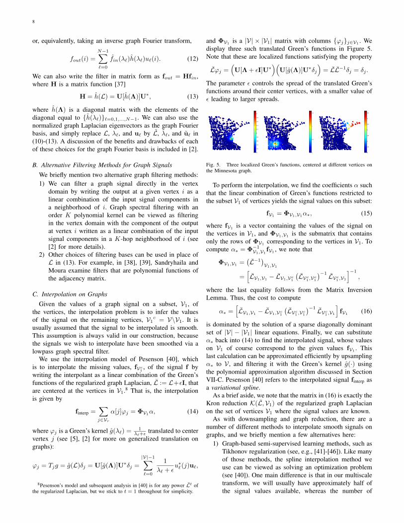
and ΦV1 is a |V| × |V1| matrix with columns {ϕj}j∈V1 . Wedisplay three such translated Green’s functions in Figure 5.Note that these are localized functions satisfying the property

Lϕj =(U[Λ + εI]U∗

)(U[g(Λ)]U∗δj

)= LL−1δj = δj .

The parameter ε controls the spread of the translated Green’sfunctions around their center vertices, with a smaller value ofε leading to larger spreads.

0

0.2

0.4

0.6

0.8

1

1.2

1.4

1.6

1.8

2

0

0.5

1

1.5

0

0.5

1

1.5

2

2.5

3

3.5

Fig. 5. Three localized Green’s functions, centered at different vertices onthe Minnesota graph.

To perform the interpolation, we find the coefficients α suchthat the linear combination of Green’s functions restricted tothe subset V1 of vertices yields the signal values on this subset:

fV1 = ΦV1,V1α∗, (15)

where fV1 is a vector containing the values of the signal onthe vertices in V1, and ΦV1,V1 is the submatrix that containsonly the rows of ΦV1 corresponding to the vertices in V1. Tocompute α∗ = Φ−1

V1,V1fV1 , we note that

ΦV1,V1 =(L−1

)V1,V1

=[LV1,V1 − LV1,Vc1

(LVc1 ,Vc1

)−1 LVc1 ,V1]−1

,

where the last equality follows from the Matrix InversionLemma. Thus, the cost to compute

α∗ =[LV1,V1 − LV1,Vc1

(LVc1 ,Vc1

)−1 LVc1 ,V1]

fV1 (16)

is dominated by the solution of a sparse diagonally dominantset of |V| − |V1| linear equations. Finally, we can substituteα∗ back into (14) to find the interpolated signal, whose valueson V1 of course correspond to the given values fV1 . Thislast calculation can be approximated efficiently by upsamplingα∗ to V , and filtering it with the Green’s kernel g(·) usingthe polynomial approximation algorithm discussed in SectionVII-C. Pesenson [40] refers to the interpolated signal finterp asa variational spline.

As a brief aside, we note that the matrix in (16) is exactly theKron reduction K(L,V1) of the regularized graph Laplacianon the set of vertices V1 where the signal values are known.

As with downsampling and graph reduction, there are anumber of different methods to interpolate smooth signals ongraphs, and we briefly mention a few alternatives here:

1) Graph-based semi-supervised learning methods, such asTikhonov regularization (see, e.g., [41]-[46]). Like manyof those methods, the spline interpolation method weuse can be viewed as solving an optimization problem(see [40]). One main difference is that in our multiscaletransform, we will usually have approximately half ofthe signal values available, whereas the number of

9

signal values available in the semi-supervised learningliterature is usually assumed to be significantly smaller.

2) Grady and Schwartz’s anisotropic interpolation solvesthe system of equations LVc1 ,Vc1 fVc1 = −LVc1 ,V1fV1 inorder to minimize fTinterpLfinterp subject to finterp(i) = f(i)for all i ∈ V .

3) Rather than using the Green’s functions as the inter-polating functions in (14), Narang et al. [47], [48]use the eigenvectors of the normalized graph Laplacianassociated with the lowest eigenvalues.

VI. A PYRAMID TRANSFORM FOR SIGNALS ON GRAPHS

We are finally ready to combine the downsampling, graphreduction, filtering, and interpolation operations from the pre-vious three sections to define a multiscale pyramid transformfor signals on graphs. After reviewing the classical Laplacianpyramid, we summarize our extension, first for a single leveland then for the whole pyramid.

A. The Classical Laplacian Pyramid

In [15], Burt and Adelson introduce the Laplacian pyramid.Originally designed with image coding in mind, the Laplacianpyramid is a multiresolution transform that is applicable toany regularly-sampled signal in time or space. A schematicrepresentation of a single level of the Laplacian pyramid isshown in Figure 6(a). At each level of the pyramid, an inputsignal x is lowpass filtered (H) and then downsampled to forma coarse approximation of the original signal. A prediction ofthe input signal is then formed by upsampling and lowpassfiltering (G) the coarse approximation. The prediction error y,i.e., the difference between the input signal and the predictionbased on the coarse approximation, is stored for reconstruc-tion. This process is iterated, with the coarse approximationthat is output at the previous level acting as the input to thenext level. The sequence

{x(i)}i=1,2,...

represents a series ofcoarse approximations of the original signal x(0) at decreasingresolutions. If, for example, the downsampling is by a factorof 2 and the original signal x(0) ∈ RN , then x(i) ∈ R2−iN .

The lowest resolution approximation, x(J), of theoriginal signal and the sequence of prediction errors,{y(i)}i=0,1,...,J−1

are stored and/or transmitted for recon-struction. Therefore, the Laplacian pyramid is an overcompletetransform, as a J-level pyramid downsampled by a factorof κ at each level maps an input of dimension N intoN(

1− 1κJ+1

1− 1κ

)transform coefficients. On the other hand, the

Laplacian pyramid has a number of desirable properties. First,perfect reconstruction of the original signal is possible forany choice of filtering operations H and G. It is easy tosee that upsampling x(j+1), filtering it by G, and summingwith the prediction error y(j) yields the finer approximationx(j). Second, the prediction errors usually have less entropythan the original signal of the same dimension, enablingfurther compression. Third, it is computationally efficient toimplement the transform, due to the hierarchical and localnature of the computations.

For some applications, the reconstruction process starts withnoisy transform coefficients, due to communication noise,

x(j) ↓ ↑H G +

x(j+1)

y(j)

1) Need to store whole Laplacian?

(a)

Interpolate from Ѵ1

to Ѵ

x(j)

L (j) Vertex Selec4on

Graph Reduc4on

m(j) L (j+1)

H(j)

x(j+1)

y(j)

m(j)

↓Ѵ1 +

(b)

x(4)

Single Level of Pyramid x(0)

L (0)

L (1)

x(1)

y(0) m(0)

Single Level of Pyramid L (2)

x(2)

y(1) m(1)

Single Level of Pyramid L (3)

x(3)

y(2) m(2)

Single Level of Pyramid

m(3)

L (4) y(3)

(c)

Fig. 6. (a) A single level of the classical Laplacian pyramid of Burt andAdelson [15]. (b) A single level of the pyramid scheme proposed for signalsdefined on graphs. The top half consisting of the graph downsampling andreduction is specific to the graph (but the same for every signal on that graph),while the bottom half is specific to each graph signal. (c) A multilevel pyramidfor signals defined on graphs.

quantization error, or other types of processing. In this case,Do and Vetterli [49], [50] show that Burt and Adelson’ssingle-level synthesis operator is not optimal in terms ofthe reconstruction error. The single-level analysis operatorthat transforms a coarse approximation x(j) into the nextcoarse approximation x(j+1) and prediction error y(j) is aframe operator (see, e.g., [51]). Frame operators have aninfinite number of left inverses, but the one that minimizesthe reconstruction error is the pseudoinverse of the analysisoperator at each level of the pyramid. In Section VI-D, we alsouse the pseudoinverse of the analysis operator as the synthesisoperator at each level of our Laplacian pyramid for signals ongraphs. Thus, we defer a more precise mathematical treatmentof the optimal reconstruction until then.

B. The Analysis Operator for a Single Level of the Pyramidfor Signals on Graphs

We now extend the classical Laplacian pyramid to a pyramidtransform for signals on graphs. At each level of the pyramid,the inputs are the current coarse approximation, x(j) ∈ RN(j)

,of the original signal, and the current graph Laplacian L(j) ∈RN(j) ×RN(j)

. We use the polarity of the largest eigenvector

10

of L(j), as described in Section III, to select the vertices of thegraph on which to form the reduced graph at resolution scalej+ 1. We denote the output of the vertex selection process bym(j) ∈ RN(j)

, where

m(j)(i) =

1, if vertex i is selected to be included in the

reduced graph0, otherwise

.

The vertex selection vector m(j) is used both to reduce thegraph and to define the downsampling and interpolation oper-ators. For graph reduction, we use Kron reduction followed byspectral sparsification, as discussed in Section IV. The graphLaplacian of the reduced graph is given by

L(j+1) = S(K(L(j),m(j)

))= S

(L(j)

V(j)1 ,V(j)

1

− L(j)

V(j)1 ,V(j)c

1

[L(j)

V(j)c

1 ,V(j)c

1

]−1

L(j)

V(j)c

1 ,V(j)1

),

where V(j)1 :=

{i ∈ {1, 2, . . . , N (j)} : m(j)(i) = 1

}and S is

the spectral sparsification operator. The reduced graph L(j+1)

and the vertex selection vector m(j), both of which need tobe stored for reconstruction, are the first two outputs of thetransform at each level of the pyramid.

The other two outputs are the coarse approximation vectorx(j+1) at the coarser resolution scale j+1, and the next predic-tion error vector y(j). The course approximation vector is com-puted in a similar fashion as in the classical Laplacian pyramid,with the filtering and downsampling operators replaced bytheir graph analogs. The downsampling operator ↓ correspondsto matrix multiplication by the matrix S

(j)d ∈ RN(j+1)×RN(j)

,where S

(j)d := [IN(j) ]V(j)

1 ,V(j) and IN(j) is an N (j) × N (j)

identity matrix. For example, if m(j) = (1, 1, 0, 0, 1, 0)T, then

S(j)d =

1 0 0 0 0 00 1 0 0 0 00 0 0 0 1 0

.Rather than upsample and filter with another lowpass filter Gas in the classical pyramid, we compute the prediction errorwith the spline interpolation method of Section V-C. Whilethis adds some additional computational cost, our experimentsshowed that this change significantly improves the predictions,and in turn the sparsity of the transform coefficients. So thesingle-level analysis operator T

(j)a : RN(j) → RN(j)+N(j+1)

isgiven by

T(j)a x(j) :=

S(j)d H(j)

IN(j) −Φ(j)V1

(Φ

(j)V1,V1

)−1

S(j)d H(j)

x(j)

=

[x(j+1)

y(j)

](17)

In (17), the filtering operator is H(j) = U(j)[h(Λ(j))]U(j)∗ .A schematic representation of a single level of the pyramid

for signals on graphs is shown in Figure 6(b). Note thatwhile we use the polarity of the largest eigenvector of thegraph Laplacian as a vertex selection method, the sparsifiedKron reduction as a graph reduction method, the eigenvectors

of the graph Laplacian as a filtering basis, and the splineinterpolation method with translated Green’s functions, othervertex selection, graph reduction, filtering, and interpolationmethods can be substituted into these blocks without affectingthe perfect reconstruction property of the scheme.

C. The Multilevel Pyramid

The multilevel pyramid for signals on graphs is shown inFigure 6(c). As in the classical case, we iterate the single-levelanalysis on the downsampled output of the lowpass channel.In (17), the filtering operators H(j) necessarily depend on theresolution scale j through their dependence on the eigenvectorsand eigenvalues of L(j). However, the filter h : [0, λ

(0)max]→ R

may be fixed across all levels of the pyramid due to property(6) of the Kron reduction, which guarantees that the spectrumof L(j) is contained in [0, λ

(0)max] for all j.9

D. Synthesis Operators for a Single Level and Optimal Re-construction

Just as is the case in the classical Laplacian pyramid, forany choices of filter h(·), we can reconstruct x(j) perfectlyfrom x(j+1) and y(j) with a single-level synthesis operator,T

(j)s : RN(j)+N(j+1) → RN(j)

, given by

T(j)s

[x(j+1)

y(j)

]:=

[Φ

(j)V1

(Φ

(j)V1,V1

)−1

IN(j)

] [x(j+1)

y(j)

].

(18)

Note that in order to apply the synthesis operator T(j)s , we

need access to both L(j) and m(j), which are used for theinterpolation.

It is straightforward to check that T(j)s T

(j)a = IN(j) ,

guaranteeing perfect reconstruction. However, once again anal-ogously to the classical Laplacian pyramid, when noise isintroduced into the stored coefficients x(j+1) and y(j), wewould like to reconstruct with the pseudoinverse of T

(j)a :

T(j)†

a :=(T(j)∗

a T(j)a

)−1

T(j)∗

a . (19)

If x(j+1) and y(j) are the noisy versions of x(j+1) andy(j), respectively, then x(j) = T

(j)†

a

[x(j+1)

y(j)

]minimizes the

reconstruction error. That is,

T(j)†

a

[x(j+1)

y(j)

]= argmin

x∈RN(j)

∣∣∣∣∣∣∣∣T(j)a x−

[x(j+1)

y(j)

]∣∣∣∣∣∣∣∣2

. (20)

For large graphs, rather than form and compute the matrixinverse in (19), it may be more computationally efficientto approximate the left-hand side of (20) with Landweberiteration [54, Theorem 6.1].

To summarize, for a multilevel pyramid for signals ongraphs that has J resolution levels, the reconstruction process

9If we include spectral sparsification in the graph reduction step, then thespectrum of L(j) is not guaranteed to be contained in [0, λ

(0)max]; however, for

large graphs, the results of [30] limit the extent to which the maximum graphLaplacian eigenvalue can increase beyond λ

(0)max. In any case, we usually

define the filters on the entire positive real line, in which case there is noissue with the length of the spectrum increasing at successive levels of thepyramid.

11

−1

−0.8

−0.6

−0.4

−0.2

0

0.2

0.4

0.6

0.8

1

−1

−0.8

−0.6

−0.4

−0.2

0

0.2

0.4

0.6

0.8

1

−1

−0.8

−0.6

−0.4

−0.2

0

0.2

0.4

0.6

0.8

1

−1

−0.8

−0.6

−0.4

−0.2

0

0.2

0.4

0.6

0.8

1

Coarse Approximations

Original Signal - x(0)

Prediction Errors

x(1) x(2) x(3)

y(0) y(1) y(2)

−1

−0.8

−0.6

−0.4

−0.2

0

0.2

0.4

0.6

0.8

1

−1

−0.8

−0.6

−0.4

−0.2

0

0.2

0.4

0.6

0.8

1

−1

−0.8

−0.6

−0.4

−0.2

0

0.2

0.4

0.6

0.8

1

Fig. 7. Three-level pyramid analysis of a piecewise-constant signal on the Minnesota road network of [52]. The number of vertices is reduced in successivecoarse approximations from N = 2642 to 1334 to 669 to 337. The overall redundancy factor of the transform in this case is 1.89.

−4

−3

−2

−1

0

1

2

3

4

−4

−3

−2

−1

0

1

2

3

4

−4

−3

−2

−1

0

1

2

3

4

−6

−5

−4

−3

−2

−1

0

1

2

Coarse Approximations

Original Signal - x(0)

Prediction Errors

x(1) x(2) x(3)

y(0) y(1) y(2)

−6

−5

−4

−3

−2

−1

0

1

2

−6

−5

−4

−3

−2

−1

0

1

2

−6

−5

−4

−3

−2

−1

0

1

2

Fig. 8. Three-level pyramid analysis of a piecewise-smooth signal on the Stanford Bunny graph of [53]. The number of vertices is reduced in successivecoarse approximations from N = 8170 to 4108 to 2050 to 1018. The overall redundancy factor of the transform in this case is 1.88.

begins with knowledge of m(0), m(1), . . ., m(J−1), L(0), L(1),. . ., L(J−1), y(0), y(1), . . ., y(J−1), and x(J). We first usem(J−1) and L(J−1) to apply T

(J−1)†

a to[

x(J)

y(J−1)

]. The result

is x(J−1). We then use m(J−2) and L(J−2) to apply T(J−2)†

a

to[x(J−1)

y(J−2)

]in order to compute x(J−2). We iterate this process

J times until we finally compute x(0), which, if no noise hasbeen introduced into the transform coefficients, is equal to theoriginal signal x(0).

E. Illustrative Examples

In Figure 7, we use the proposed pyramid transform toanalyze a piecewise-constant signal (the Fiedler vector u1) onthe Minnesota road network of [52]. After each Kron reductionat stage j, we use the spectral sparsification of Algorithm 1with Q set to the integer closest to 4N (j) log(N (j)). The graphspectral filter is h(λ`) := 0.5

0.5+λ`, and we take ε = 0.005

to form the regularized Laplacian for interpolation. We see

that the prediction error coefficients are extremely sparse, andthose with non-zero magnitudes are concentrated around thediscontinuity in the graph signal.

In Figure 8, we apply the transform to a piecewise smoothsignal on the Stanford Bunny graph [53] with 8170 vertices.The signal is comprised of two different polynomials of thecoordinates: x2 + y − 2z on the head and ears of the bunny,and x − y + 3z2 − 5 on the lower body, where (x, y, z) arethe physical coordinates of each vertex. Since the graph islarger and the graph Laplacian spectrum is wider than theprevious example, we take Q to be the integer closest to16N (j) log(N (j)), the lowpass filter to be h(λ`) := 5

5+λ`,

and ε = 0.05 for interpolation.

As a compression example, we hard threshold the 15346pyramid transform coefficients of the signal, keeping only the2724 with the largest magnitudes (approximately 1/3 the sizeof the original signal) and setting the rest to 0. Reconstructionof the signal from the thresholded coefficients yields an error

12

−6

−5

−4

−3

−2

−1

0

1

2

(a)

0 2000 4000 6000 8000 10000 12000 14000 160000

1

2

3

4

5

6

(b)

−6

−5

−4

−3

−2

−1

0

1

2

(c)

Fig. 9. Compression example. (a) The original piecewise-smooth signal witha discontinuity on the Stanford bunny [53]. (b) The sorted magnitudes of the15346 pyramid transform coefficients. (c) The reconstruction from the 2724coefficients with the largest magnitudes, using the least squares synthesis (19).

||freconstruction−f ||2||f ||2 of 0.145 with the direct synthesis (18), and an

error of 0.086 with the least squares synthesis (19). Figure9 shows the original signal, the sorted magnitudes of thetransform coefficients, and the reconstruction with the leastsquares synthesis operator.

F. Comparison with Other Transforms

A thorough comparison of our proposed pyramid transformto other multiscale transforms for signals on graphs investi-gating which transforms work best on which types of graphsignals in which signal processing tasks is beyond the scopeof this work. However, in this section, we present a fewillustrative numerical denoising and compression experimentswith our proposed pyramid transform and other multiscaletransforms for graph signals.

First, one qualitative difference between the proposed trans-form and many other multiscale transforms for graph signalsis that our transform outputs both a multiresolution of graphsand a graph signal multiresolution residing on that graphmultiresolution. While less important for numerical graphsignal processing and machine learning tasks, this featureis especially beneficial for multiscale visualization of graphsignals (e.g., the sequence of coarse approximations in the toprow of Figure 8). A few other transforms such as the critically-sampled spline wavelet filter banks [9] share this feature, butmany others such as the spectral graph wavelets [5] and thespatial graph wavelets [3] do not yield such a sequence ofcoarse approximations at different resolution levels.

Second, the dictionary atoms we construct tend to bejointly localized in the vertex domain and the graph spectraldomain. The hope is that such atoms are able to sparselyrepresent various classes of graph signals, such as those thatare piecewise smooth with discontinuities. Unfortunately, thereis little theory to date relating mathematical classes of graphsignals to the sparsity of particular transform coefficients. Oneinitial exploration into this line of investigation for the caseof spectral graph wavelets is presented in [55]. We conduct afew numerical experiments below to explore the decay of thetransform coefficients for different types of signals.

1) Denoising: We start by repeating the denoising exper-iment of [56, Section VI.D] on the Minnesota road networkof [52].10 We add white Gaussian noise with varying standard

10To replicate the experiment with our transform, we leveraged theMATLAB code of [56], which is publicly available at http://tanaka.msp-lab.org/software.

−1.5

−1

−0.5

0

0.5

1

1.5

(a)

−1.5

−1

−0.5

0

0.5

1

1.5

(b)

−1.5

−1

−0.5

0

0.5

1

1.5

(c)

Fig. 10. Denoising example. (a) Piecewise constant signal on the Minnesotagraph. (b) Noisy observation with σ = 1

2. (c) Denoised signal reconstructed

after hard thresholding the prediction errors of a two-level pyramid transform.

TABLE IDENOISING RESULTS ON THE MINNESOTA TRAFFIC GRAPH: SNR (DB)

σ noisy 1-level pyramid 2-level pyramid reference range1/32 30.10 34.81 34.30 31.44 - 35.081/16 24.08 28.60 27.35 25.61 - 29.341/8 18.06 22.84 20.34 19.97 - 23.171/4 12.04 17.00 15.85 14.19 - 17.631/2 6.02 12.77 13.51 8.50 - 12.311 0.00 7.96 10.46 2.63 - 8.82

Redundancy - 1.50 1.76 1.00 - 4.00

deviations to the piecewise-constant reference signal from [19]shown in Figure 10(a). As in [56], we compute the pyramidtransform coefficients, hard threshold the prediction errors ata threshold of 3σ, and reconstruct a denoised signal (shownin Figure 10(c) for the case of σ = 1

2 ) from the coarseapproximation coefficients and the thresholded prediction errorcoefficients. We use the same parameters as in Figure 7 toconstruct the graph multiresolution. We take the graph spectralfilters to be h(λ`) := 1

1+λ`, and take ε = 0.005 to form

the regularized Laplacian for interpolation. In Table I, wecompare the denoising results for a one-level and two-leveltransform to a reference range of results attained by differenttransforms in [56], including variants of the biorthogonalgraph filter banks of [57], the oversampled graph filter banksof [56], and the spectral graph wavelet transform of [5].Qualitatively comparing the denoised signal in Figure 10(c) toits counterparts in [56, Fig. 15], it appears that our denoisedsignal is smoother with respect to the graph structure, withmore of the errors clustered around the discontinuity in thepiecewise-constant signal.

2) Compression: Next, we repeat the compression exper-iment of Figure 9 on three different types of graph signals.First, we consider a piecewise-smooth signal with discontinu-ities. We compose the signal in Figure 11(a) on the 500 vertexrandom sensor network from Figure 4 by segmenting the graphinto four strips and restricting two different polynomials ofthe coordinates to the different sections of the graph. Thefirst polynomial 0.5 − 2x is restricted to the first and thirddiagonal strips, counting from the upper right, and the secondpolynomial 0.5+ x2 + y2 is restricted to the second and fourthstrips (the latter of which is the lower left corner), where (x, y)are the physical coordinates of each vertex. We sum the twocomponents to form the signal.

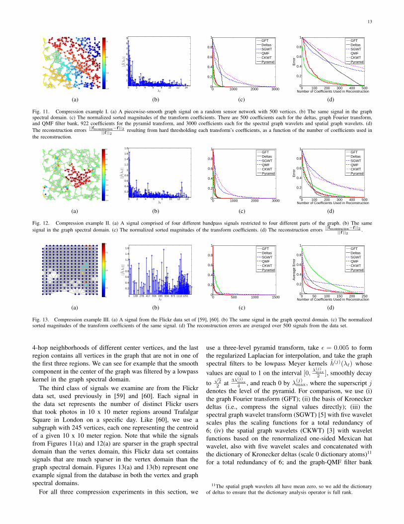
The second signal, shown in Figure 12(a), is from [58, Fig.16(c)]. It is formed by generating four different random signalson the graph, filtering them with different bandpass filters,restricting each of the bandpass signals to different regions ofthe graph, and then summing them. The first three regions are

13

−1.5

−1

−0.5

0

0.5

1

1.5

(a)

0 2 4 6 8 10 12 14

1

2

3

4

5

6

7

8

9

λ`

|f(λ

`)|

(b)

0 1000 2000 30000

0.2

0.4

0.6

0.8

1

GFTDeltasSGWTQMFCKWTPyramid

(c)

0 100 200 300 400 5000

0.2

0.4

0.6

0.8

1

Number of Coefficients Used in Reconstruction

Err

or


(d)

Fig. 11. Compression example I. (a) A piecewise-smooth graph signal on a random sensor network with 500 vertices. (b) The same signal in the graphspectral domain. (c) The normalized sorted magnitudes of the transform coefficients. There are 500 coefficients each for the deltas, graph Fourier transform,and QMF filter bank, 922 coefficients for the pyramid transform, and 3000 coefficients each for the spectral graph wavelets and spatial graph wavelets. (d)The reconstruction errors ||freconstruction−f ||2

||f ||2resulting from hard thresholding each transform’s coefficients, as a function of the number of coefficients used in

the reconstruction.

−0.5

−0.4

−0.3

−0.2

−0.1

0

0.1

0.2

0.3

0.4

0.5

(a)

0 2 4 6 8 10 12 14

0.2

0.4

0.6

0.8

1

1.2

1.4

1.6

1.8

λ`

|f(λ

`)|

(b)

0 1000 2000 30000

0.2

0.4

0.6

0.8

1


(c)

0 100 200 300 400 5000

0.2

0.4

0.6

0.8

1


Err

or


(d)

Fig. 12. Compression example II. (a) A signal comprised of four different bandpass signals restricted to four different parts of the graph. (b) The samesignal in the graph spectral domain. (c) The normalized sorted magnitudes of the transform coefficients. (d) The reconstruction errors ||freconstruction−f ||2

||f ||2.

0

0.5

1

1.5

2

2.5

3

(a)

0 139 278 417 556 695 834 973 1112 1251

0.2

0.4

0.6

0.8

1

1.2

1.4

1.6

λ`

|f(λ

`)|

(b)

0 500 1000 15000

0.2

0.4

0.6

0.8

1


(c)

0 50 100 150 200 2500

0.2

0.4

0.6

0.8

1


Ave

rage

Err

or


(d)

Fig. 13. Compression example III. (a) A signal from the Flickr data set of [59], [60]. (b) The same signal in the graph spectral domain. (c) The normalizedsorted magnitudes of the transform coefficients of the same signal. (d) The reconstruction errors are averaged over 500 signals from the data set.

4-hop neighborhoods of different center vertices, and the lastregion contains all vertices in the graph that are not in one ofthe first three regions. We can see for example that the smoothcomponent in the center of the graph was filtered by a lowpasskernel in the graph spectral domain.

The third class of signals we examine are from the Flickrdata set, used previously in [59] and [60]. Each signal inthe data set represents the number of distinct Flickr usersthat took photos in 10 x 10 meter regions around TrafalgarSquare in London on a specific day. Like [60], we use asubgraph with 245 vertices, each one representing the centroidof a given 10 x 10 meter region. Note that while the signalsfrom Figures 11(a) and 12(a) are sparser in the graph spectraldomain than the vertex domain, this Flickr data set containssignals that are much sparser in the vertex domain than thegraph spectral domain. Figures 13(a) and 13(b) represent oneexample signal from the database in both the vertex and graphspectral domains.

For all three compression experiments in this section, we

use a three-level pyramid transform, take ε = 0.005 to formthe regularized Laplacian for interpolation, and take the graphspectral filters to be lowpass Meyer kernels h(j)(λ`) whosevalues are equal to 1 on the interval [0,

λ(j)max

2 ], smoothly decay

to√

22 at 3λ(j)

max

4 , and reach 0 by λ(j)max, where the superscript j

denotes the level of the pyramid. For comparison, we use (i)the graph Fourier transform (GFT); (ii) the basis of Kroneckerdeltas (i.e., compress the signal values directly); (iii) thespectral graph wavelet transform (SGWT) [5] with five waveletscales plus the scaling functions for a total redundancy of6; (iv) the spatial graph wavelets (CKWT) [3] with waveletfunctions based on the renormalized one-sided Mexican hatwavelet, also with five wavelet scales and concatenated withthe dictionary of Kronecker deltas (scale 0 dictionary atoms)11

for a total redundancy of 6; and the graph-QMF filter bank

11The spatial graph wavelets all have mean zero, so we add the dictionaryof deltas to ensure that the dictionary analysis operator is full rank.

14

transform (QMF) [19].12 Note that the graph-QMF transformonly uses the adjacency matrix structure, and not the weightsof the graphs.

Figures 11(c), 12(c), and 13(c) show the decay of themagnitudes of the transform coefficients for the signals shownin Figures 11(a), 12(a), and 13(a), respectively. In these plots,for each transform and signal pair, we normalize the sortedmagnitudes by dividing every transform coefficient of thatpair by the largest magnitude coefficient of that pair. For thiscompression experiment, we keep the M coefficients withthe largest magnitudes, set the rest to 0, and reconstruct thesignal from the thresholded transform coefficients. For a faircomparison, for all transforms, we perform least squares re-construction by applying the pseudoinverse of the analysis op-erator to the thresholded coefficients. In Figures 11(d), 12(d),and 13(d), we show the reconstruction errors ||freconstruction−f ||2

||f ||2for varying values of M , the number of coefficients used inthe reconstruction. Note that the errors in 13(d) are averagedover 500 different signals from the data set. We see thatour proposed pyramid transform works reasonably well forcompression for all three signal models.

VII. IMPLEMENTATION APPROXIMATIONS ANDCOMPUTATIONAL COMPLEXITY

In their seminal paper on the Laplacian pyramid, Burt andAdelson [15] write, “The coding scheme outlined above willbe practical only if the required filtering computations can beperformed with an efficient algorithm.” In the same spirit, wemention here some approximation techniques to improve thecomputational efficiency of the proposed transform.

As described analytically, the transform relies on repeatedeigendecompositions of the graph Laplacian for filtering,downsampling, and graph reduction. However, for large graphs(with tens of thousands or more vertices), computing fulleigendecompositions is computationally expensive and maynot be possible. This is because general-purpose routines forcomputing the full eigendecomposition have computationalcomplexities of O(N3). Accordingly, two common themesrunning through this section are (i) to avoid computing fulleigendecompositions, and (ii) to take advantage of (and pre-serve) the sparsity of the graph Laplacian whenever possible.

A. Power Method for Computing the Largest Eigenvector

To compute the largest eigenvector of an N × N graphLaplacian, we can use the power method, which generatesa sequence of vectors

{x(k)

}k=0,1,...

through the followingrecursion:

x(k) =Lx(k−1)

‖Lx(k−1)‖2. (21)

If λmax > λN−2 and 〈x(0),umax〉 6= 0, then the sequenceof vectors

{x(k)

}k=0,1,...

generated by the power methodconverges to umax [61, Chapter 8.2.1]. Convergence is fasterthe smaller the ratio λN−2

λmaxis, and it may be accelerated by

12The MATLAB code for the graph-QMF filter bank is publicly availableat http://biron.usc.edu/wiki/index.php/Graph Filterbanks.

subtracting a multiple of the identity matrix from L to shiftthe spectrum [62, Chapter 4.1]. The computational cost of (21)is dominated by the O(|E|) matrix-vector multiplication bythe matrix L. In sparse graphs, |E| may grow linearly withN , making this an efficient method to compute the largesteigenvector. The condition 〈x(0),umax〉 6= 0 is satisfied byalmost any x(0) chosen at random [62, Chapter 5.1]. If thelargest eigenvalue is not simple, the power method convergesto a vector in the largest eigenspace, but this vector is notunique. For downsampling purposes, we only need to computeenough iterations to approximate the polarities of the largesteigenvector components, as opposed to their precise values.

B. Efficient Implementation of Kron Reduction and Storage ofReduced Graph Information

Full computation of the Kron-reduced Laplacian K (L,V1)in (3) can be computationally expensive (O(N3) with naivemethods that do not take advantage of the structure of LVc1 ,Vc1 ).One option is to not actually compute the entire reducedgraph Laplacian, but rather to form an operator to do matrix-vector multiplication with the matrix being the Kron-reducedLaplacian (see, e.g., [63] or the function MatCreateSchurCom-plement in PETSc [64]). The drawback of doing so is thatwe cannot plot reduced graphs and coarser approximationsas in Figure 7; however, such a method is well-suited forsituations such as compression or regularization where we areonly interested in computing transform coefficients.

In some cases, we may actually want to compute and storeall of the graph Laplacians L(0),L(1), . . . ,L(J−1) as partof a multilevel transform. If we are repeatedly applying thetransform to different signals on the same graph (e.g., a fixedtransportation network), then the overhead of computing andstoring this sequence of reduced graph Laplacians is sharedacross all of the applications of the transform. On the otherhand, if the graph is completely different for every graph signal(e.g., some graph-based image processing methods), then effi-cient storage and reconstruction of the graph Laplacians is animportant computational consideration. In either case, becausethe Schur complement is often dense even if L is sparse, it canalso be computationally expensive to store LKron−reduced forlarge graphs. The addition of a sparsification step after eachKron reduction reduces the storage requirements, as well as thecomplexity of subsequent computations. One interesting openquestion is whether we can avoid storing the entire sequence ofLaplacians, but rather store the coarsest Laplacian and someadditional side information, and still be able to recover theentire sequence in reverse order.

C. Approximate Graph Spectral Filtering

The Chebyshev polynomial approximation method, whichis introduced in [5] and discussed further in [65], can beused to speed up graph spectral filtering operations. Thatmethod computes an approximately filtered signal Hf throughrepeated matrix-vector multiplication by the matrix L at acomputational cost of O(K|E|), where K is the order of theChebyshev polynomial approximation. Therefore, for a sparsegraph, it is far more efficient to compute Hf than Hf .

15

D. Computational ComplexityTo summarize, we can break the computational complexity

down into two parts: the first for computing the multiresolu-tion of graphs and the second for analyzing signals on thatmultiresolution of graphs with the filtering and interpolationoperations. As mentioned above, the overhead of computingand storing the multiresolution of graphs is often shared acrossapplications of the transform to many different signals on thesame graph.

The bottleneck for the signal analysis portion of the mul-tiscale pyramid transform we proposed in Section VI is theinterpolation step (16). Recent advances in solving such sparse,symmetric, diagonally dominant systems of equations providemethods to reduce the computational cost from O(|E|N) downto O(|E| log2N), or even faster [14], [32], [66], [67]. Theseadvances also enable the spectral sparsification step to be donein nearly linear time with respect to the number of edges in theoriginal graph. To compute the full graph multiresolution forvisualization, the bottleneck is the Kron reduction step (3).Here, we can again take advantage of methods for solvingsymmetric diagonally dominant systems of linear equations innearly linear time in the number of edges. For example, wecan use the LAMG solver of [32] to compute L−1

Vc1 ,Vc1LVc1 ,i,

for each i in V1. Both the time to setup the problem (create asequence of coarse-grained Laplacians) and the time to solvethe problem are empirically shown in [32] to be linear in thenumber of edges. Since we have to solve the problem for eachcolumn of LVc1 ,V1 , the overall computational cost of the Kronreduction should be on the order O(|E|N), but at least weonly need to perform the setup portion once for LVc1 ,Vc1 .

VIII. CONCLUSION

Our main contribution in this work has been to present anew framework for a multiscale pyramid transform for graphsignals that is centered around the four fundamental opera-tions of graph downsampling, graph reduction, graph spectralfiltering, and interpolation of graph signals. Our frameworkis modular, so we can easily substitute different choices forthese fundamental operations (e.g., choose a different graphdownsampling operator in the Laplacian pyramid of Figure6). We hope this framework inspires new choices for andanalyses of these fundamental operations. For example, sincethe presentation of an initial version of our work here, [68]has presented a new method for graph downsampling in thecontext of signal processing, and [69] has presented a newmethod for graph reduction that preserves the eigenvalues fromone graph to the next in the graph multiresolution.

The interplay between the four operations is important andless well understood in the context of graph signal processing.Further empirical and theoretical investigations into how thejoint choice of these operations affects properties such asthe joint localization of the resulting dictionary atoms in thevertex-frequency space, as well as the sparsity of transformcoefficients for different classes of graph signals is an im-portant line of future work. Another natural offshoot of thiswork would be to combine these fundamental graph signalprocessing operations in different manners to generate othermultiscale transforms such as critically sampled filter banksand lifting transforms.

REFERENCES

[1] M. J. Faraji, “A Laplacian pyramid scheme in graph signal processing,”Master’s thesis, Ecole Polytechnique Federale de Lausanne (EPFL),Lausanne, Switzerland, Jun. 2011.

[2] Shuman, D. I, S. K. Narang, P. Frossard, A. Ortega, and P. Van-dergheynst, “The emerging field of signal processing on graphs: Ex-tending high-dimensional data analysis to networks and other irregulardomains,” IEEE Signal Process. Mag., vol. 30, pp. 83–98, May 2013.

[3] M. Crovella and E. Kolaczyk, “Graph wavelets for spatial trafficanalysis,” in Proc. IEEE INFOCOM, vol. 3, Mar. 2003, pp. 1848–1857.

[4] R. R. Coifman and M. Maggioni, “Diffusion wavelets,” Appl. Comput.Harmon. Anal., vol. 21, no. 1, pp. 53–94, 2006.

[5] D. K. Hammond, P. Vandergheynst, and R. Gribonval, “Wavelets ongraphs via spectral graph theory,” Appl. Comput. Harmon. Anal., vol. 30,no. 2, pp. 129–150, Mar. 2011.

[6] M. Jansen, G. P. Nason, and B. W. Silverman, “Multiscale methods fordata on graphs and irregular multidimensional situations,” J. R. Stat.Soc. Ser. B Stat. Methodol., vol. 71, no. 1, pp. 97–125, 2009.

[7] S. K. Narang and A. Ortega, “Lifting based wavelet transforms ongraphs,” in Proc. APSIPA ASC, Sapporo, Japan, Oct. 2009, pp. 441–444.

[8] ——, “Local two-channel critically sampled filter-banks on graphs,” inProc. Int. Conf. Image Process., Hong Kong, Sep. 2010, pp. 333–336.

[9] V. N. Ekambaram, G. C. Fanti, B. Ayazifar, and K. Ramchandran,“Critically-sampled perfect-reconstruction spline-wavelet filter banks forgraph signals,” in Proc. Glob. Conf. Signal Inf. Process., Austin, TX,Dec. 2013, pp. 475–478.

[10] M. Gavish, B. Nadler, and R. R. Coifman, “Multiscale wavelets on trees,graphs and high dimensional data: Theory and applications to semisupervised learning,” in Proc. Int. Conf. Mach. Learn., Haifa, Israel,Jun. 2010, pp. 367–374.

[11] S.-H. Teng, “Coarsening, sampling, and smoothing: Elements of themultilevel method,” in Parallel Processing, IMA Volumes in Mathematicsand its Applications, 105. Springer Verlag, 1999, pp. 247–276.

[12] A. Brandt, “Multiscale scientific computation: Review 2001,” in Mul-tiscale and Multiresolution Methods: Theory and Applications, LectureNotes in Comput. Sci. 20, T. J. Barth, T. Chan, and R. Haimes, Eds.Springer-Verlag, 2001, pp. 3–96.

[13] D. Ron, I. Safro, and A. Brandt, “Relaxation-based coarsening andmultiscale graph organization,” Multiscale Model. Simul., vol. 9, no. 1,pp. 407–423, Sep. 2011.

[14] N. K. Vishnoi, Lx = b, ser. Foundations and Trends in ComputerScience. Now Publishers, 2013.

[15] P. J. Burt and E. H. Adelson, “The Laplacian pyramid as a compactimage code,” IEEE Trans. Commun., vol. 31, pp. 532–540, Apr. 1983.

[16] R. Roth, “On the eigenvectors belonging to the minimum eigenvalueof an essentially nonnegative symmetric matrix with bipartite graph,”Linear Algebra Appl., vol. 118, pp. 1–10, Jun. 1989.

[17] T. Bıyıkoglu, J. Leydold, and P. F. Stadler, Laplacian Eigenvectors ofGraphs. Lecture Notes in Mathematics, vol. 1915, Springer, 2007.

[18] S. K. Narang and A. Ortega, “Downsampling graphs using spectraltheory,” in Proc. IEEE Int. Conf. Acc., Speech, and Signal Process.,Prague, Czech Republic, May 2011, pp. 4208–4211.

[19] ——, “Perfect reconstruction two-channel wavelet filter banks for graphstructured data,” IEEE Trans. Signal Process., vol. 60, no. 6, pp. 2786–2799, Jun. 2012.

[20] G. Shen and A. Ortega, “Tree-based wavelets for image coding: Orthog-onalization and tree selection,” in Proc. Picture Coding Symp., Chicago,IL, May 2009, pp. 1–4.

[21] B. Aspvall and J. R. Gilbert, “Graph coloring using eigenvalue decom-position,” SIAM J. Alg. Disc. Meth., vol. 5, no. 4, pp. 526–538, 1984.

[22] U. von Luxburg, “A tutorial on spectral clustering,” Stat. Comput.,vol. 17, no. 4, pp. 395–416, 2007.

[23] E. B. Davies, G. M. L. Gladwell, J. Leydold, and P. F. Stadler, “Discretenodal domain theorems,” Lin. Algebra Appl., vol. 336, no. 1-3, pp. 51–60, Oct. 2001.

[24] G. Berkolaiko, “A lower bound for nodal count on discrete and metricgraphs,” Commun. Math. Phys., vol. 278, no. 3, pp. 803–819, 2008.

[25] I. Oren, “Nodal domain counts and the chromatic number of graphs,”J. Phys. A: Math. Theor., vol. 40, no. 32, pp. 9825–9832, 2007.

[26] S. T. Barnard and H. D. Simon, “Fast multilevel implementation ofrecursive spectral bisection for partitioning unstructured problems,”Concurrency: Practice and Experience, vol. 6, no. 2, pp. 101–117, Apr.1994.

16

[27] F. Dorfler and F. Bullo, “Kron reduction of graphs with applicationsto electrical networks,” IEEE Trans. Circuits and Systems-I: RegularPapers, vol. 60, no. 1, pp. 150–163, Jan. 2013.

[28] F. Zhang, The Schur Complement and its Applications. Springer, 2005.[29] D. J. Klein and M. Randic, “Resistance distance,” J. Math. Chem.,

vol. 12, pp. 81–95, 1993.[30] D. A. Spielman and N. Srivastava, “Graph sparsification by effective

resistances,” SIAM J. Comput., vol. 40, no. 6, pp. 1913–1926, 2011.[31] S. Lafon and A. B. Lee, “Diffusion maps and coarse-graining: A unified

framework for dimensionality reduction, graph partitioning, and dataset parameterization,” IEEE Trans. Pattern Anal. Mach. Intell., vol. 28,no. 9, pp. 1393–1403, Sep. 2006.

[32] O. E. Livne and A. Brandt, “Lean algebraic multigrid (LAMG): Fastgraph Laplacian linear solver,” SIAM J. Sci. Comput., vol. 34, no. 4, pp.B499–B522, 2012.

[33] G. Karypis and V. Kumar, “A fast and high quality multilevel schemefor partitioning irregular graphs,” SIAM J. Sci. Comput., vol. 20, no. 1,pp. 359–392, 1998.

[34] I. Dhillon, Y. Guan, and B. Kulis, “Weighted graph cuts withouteigenvectors a multilevel approach,” IEEE Trans. Pattern Anal. Mach.Intell., vol. 29, no. 11, pp. 1944–1957, Nov. 2007.

[35] C. Walshaw, “The graph partitioning archive,”http://staffweb.cms.gre.ac.uk/∼wc06/partition/.

[36] F. K. Chung, Spectral Graph Theory. Vol. 92 of the CBMS RegionalConference Series in Mathematics, AMS Bokstore, 1997.

[37] N. J. Higham, Functions of Matrices. Society for Industrial and AppliedMathematics, 2008.

[38] A. Sandryhaila and J. M. F. Moura, “Discrete signal processing ongraphs,” IEEE. Trans. Signal Process., vol. 61, no. 7, pp. 1644–1656,Apr. 2013.

[39] ——, “Discrete signal processing on graphs: Frequency analysis,” IEEE.Trans. Signal Process., vol. 62, no. 12, pp. 3042–3054, Jun. 2014.

[40] I. Pesenson, “Variational splines and Paley-Wiener spaces on combina-torial graphs,” Constr. Approx., vol. 29, no. 1, pp. 1–21, Feb. 2009.

[41] M. Belkin, I. Matveeva, and P. Niyogi, “Regularization and semi-supervised learning on large graphs,” in Learn. Theory, ser. Lect. NotesComp. Sci. Springer-Verlag, 2004, pp. 624–638.

[42] A. J. Smola and R. Kondor, “Kernels and regularization on graphs,” inProc. Ann. Conf. Comp. Learn. Theory, ser. Lect. Notes Comp. Sci.,B. Scholkopf and M. Warmuth, Eds. Springer, 2003, pp. 144–158.

[43] D. Zhou and B. Scholkopf, “Regularization on discrete spaces,” in Pat-tern Recogn., ser. Lect. Notes Comp. Sci., W. G. Kropatsch, R. Sablatnig,and A. Hanbury, Eds. Springer, 2005, vol. 3663, pp. 361–368.

[44] X. Zhu and Z. Ghahramani, “Semi-supervised learning using Gaussianfields and harmonic functions,” in Proc. Int. Conf. Mach. Learn.,Washington, D.C., Aug. 2003, pp. 912–919.

[45] D. Zhou, O. Bousquet, T. N. Lal, J. Weston, and B. Scholkopf, “Learningwith local and global consistency,” in Adv. Neural Inf. Process. Syst.,S. Thrun, L. Saul, and B. Scholkopf, Eds., vol. 16. MIT Press, 2004,pp. 321–328.

[46] O. Chapelle, B. Scholkopf, and A. Zien, Eds., Semi-Supervised Learning.MIT Press, 2006.

[47] S. K. Narang, A. Gadde, and A. Ortega, “Signal processing techniquesfor interpolation in graph structured data,” in Proc. IEEE Int. Conf. Acc.,Speech, and Signal Process., Vancouver, BC, May 2013, pp. 5445–5449.

[48] ——, “Localized iterative methods for interpolation of graph structureddata,” in Proc. IEEE Glob. Conf. Signal and Inform. Process., Austin,TX, Dec. 2013, pp. 491–494.

[49] M. N. Do and M. Vetterli, “Frame reconstruction of the Laplacianpyramid,” in Proc. IEEE Int. Conf. Acc., Speech, and Signal Process.,vol. 6, Salt Lake City, Utah, May 2001, pp. 3641–3644.

[50] ——, “Framing pyramids,” IEEE Trans. Signal Processing, vol. 51,no. 9, pp. 2329–2342, Sep. 2003.

[51] O. Christensen, Frames and Bases. Birkhauser, 2008.[52] D. Gleich, “The MatlabBGL Matlab library,”

http://www.cs.purdue.edu/homes/dgleich/packages/matlab bgl/index.html.[53] Stanford University Computer Graphics Laboratory, “The Stanford 3D

Scanning Repository,” http://graphics.stanford.edu/data/3Dscanrep/.[54] H. W. Engl, M. Hanke, and A. Neubauer, Regularization of Inverse

Problems. Kluwer Academic Publishers, 1996.[55] B. Ricaud, D. I Shuman, and P. Vandergheynst, “On the sparsity

of wavelet coefficients for signals on graphs,” in SPIE Wavelets andSparsity, San Diego, California, Aug. 2013.

[56] A. Sakiyama and Y. Tanaka, “Oversampled graph Laplacian matrix forgraph filter banks,” IEEE Trans. Signal Process., vol. 62, no. 24, pp.6425–6437, Dec. 2014.

[57] S. K. Narang and A. Ortega, “Compact support biorthogonal waveletfilterbanks for arbitrary undirected graphs,” IEEE Trans. Signal Process.,vol. 61, no. 19, pp. 4673–4685, Oct. 2013.

[58] D. I Shuman, B. Ricaud, and P. Vandergheynst, “Vertex-frequencyanalysis on graphs,” Appl. Comput. Harmon. Anal., Feb. 2015.

[59] X. Dong, A. Ortega, P. Frossard, and P. Vandergheynst, “Inference ofmobility patterns via spectral graph wavelets,” in Proc. IEEE Int. Conf.Acc., Speech, and Signal Process., Vancouver, Canada, May 2013, pp.3118–3122.

[60] D. Thanou, D. I Shuman, and P. Frossard, “Learning parametric dic-tionaries for signals on graphs,” IEEE Trans. Signal Process., vol. 62,no. 15, pp. 3849–3862, Aug. 2014.

[61] G. H. Golub and C. F. Van Loan, Matrix Computations. The JohnsHopkins University Press, 1996.

[62] D. S. Watkins, The Matrix Eigenvalue Problem: GR and Krylov Sub-space Methods. Society for Industrial and Applied Mathematics, 2007.

[63] Y. Saad, Iterative Methods for Sparse Linear Systems. SIAM, 2003.[64] S. Balay, J. Brown, K. Buschelman, W. D. Gropp, D. Kaushik, M. G.

Knepley, L. C. McInnes, B. F. Smith, and H. Zhang, “PETSc Web page,”2013, http://www.mcs.anl.gov/petsc.

[65] D. I Shuman, P. Vandergheynst, and P. Frossard, “Chebyshev polynomialapproximation for distributed signal processing,” in Proc. Int. Conf.Distr. Comput. Sensor Sys., Barcelona, Spain, Jun. 2011.

[66] I. Koutis, G. L. Miller, and R. Peng, “Approaching optimality for solvingSDD linear systems,” in Proc. IEEE Symp. Found. Comp. Sci., LasVegas, NV, Oct. 2010, pp. 235–244.

[67] D. A. Spielman, “Laplacian linear equations, graphsparsification, local clustering, low-stretch trees, etc.”http://www.cs.yale.edu/homes/spielman/precon/precon.html.

[68] H. Q. Nguyen and M. N. Do, “Downsampling of signals on graphs viamaximum spanning trees,” IEEE Trans. Signal Process., vol. 63, no. 1,pp. 182–191, Jan. 2015.

[69] P. Liu, X. Wang, and Y. Gu, “Coarsening graph signal with spectralinvariance,” in Proc. IEEE Int. Conf. Acc., Speech, and Signal Process.,Florence, Italy, May 2014, pp. 1070–1074.

A Multiscale Pyramid Transform for Graph Signals Multiscale Pyramid Transform for Graph Signals ......

Documents

Transcript of A Multiscale Pyramid Transform for Graph Signals Multiscale Pyramid Transform for Graph Signals ......