University of Nevada, Reno

A Multi-Functional Robot For Civil Infrastructure Inspection

A thesis submitted in partial fulfillment of therequirements for the degree of Master of Science in

Computer Science & Engineering

by

Tuan D. Le

Dr. Hung M. La - Thesis AdvisorMay 2017

i

Abstract

This thesis focuses on designing and building a robotic system for civil infrastruc-

ture inspections. The robot is equipped with two non-destructive-evaluation (NDE)

types of sensors: a ground penetrating (GPR) sensor and two electrical resistiv-

ity (ER) sensors. For localization, the robot employs an extended Kalman filter

(EKF)-based approach using global positioning system (GPS) signal. Differ from

its predecessor, the currently built robot is capable of localizing and navigating in

GPS-denied environments by using a visual inertial odometry method with a stereo

camera. In addition, the robot can build an elevation map of its surrounding areas

using a PrimeSence camera for obstacle avoidance.

ii

Acknowledgments

This thesis research is supported by the National Science Foundation under grant

NSF-IIP-ICoprs #1639092, the University of Nevada, Reno, and the INSPIRE Uni-

versity Transportation Center. Financial support for the INSPIRE University Trans-

portation Center was provided by the U.S. Department of Transportation Office of

the Assistant Secretary for Research and Technology (USDOT/OST-R) under grant

agreement No. 69A3551747126 and by participating state departments of transporta-

tion.

The views, opinions, findings and conclusions reflected in this presentation are the

responsibility of the presenter only and do not represent the official policy or position

of the USDOT/OST-R, NSF or any State or other entity.

I would like to thank my advisor, Dr. Hung La, who provided advices and supports

to help me finish my study.

I would like to express my gratitude to my committee members, Dr. George Bebis

and Dr. Hao Xu, for the precious time and effort which you have put in to review

this thesis and for providing advice along the way.

I would also like to thank my partners, Nhan Pham and Quynh Tran, for their

endless inspirations during my difficult times.

Finally I would like to thank my amazing wife, Iris, who has decidedly sacrificed

everything to support me. I could not have done this without her.

iii

Dedication

Dedicated to my parents.

iv

Table of Contents

1 Thesis Introduction, Contribution, and Content 1

1.1 Introduction . . . . . . . . . . . . . . . . . . . . . . . . . . . . . . . . 1

1.2 Contribution . . . . . . . . . . . . . . . . . . . . . . . . . . . . . . . . 2

1.3 Content . . . . . . . . . . . . . . . . . . . . . . . . . . . . . . . . . . 3

2 Background 4

2.1 Half-cell Potential (HCP) Method . . . . . . . . . . . . . . . . . . . . 5

2.2 Impact Echo (IE) . . . . . . . . . . . . . . . . . . . . . . . . . . . . . 5

2.3 Electrical Resistivity (ER) . . . . . . . . . . . . . . . . . . . . . . . . 5

2.4 Ground Penetrating Radar (GPR) . . . . . . . . . . . . . . . . . . . . 6

2.5 Related Work and Motivation to Develop A New Inspection System . 7

2.6 Summary . . . . . . . . . . . . . . . . . . . . . . . . . . . . . . . . . 10

3 Mechanical Design, Its Implementation and Sensors 11

3.1 System Design and Implmentation . . . . . . . . . . . . . . . . . . . 11

3.2 Ground Penetrating Radar and Electric Resistivity . . . . . . . . . . 14

3.3 Stereo camera and IMU . . . . . . . . . . . . . . . . . . . . . . . . . 17

3.4 PrimeSense camera . . . . . . . . . . . . . . . . . . . . . . . . . . . . 18

3.5 Summary . . . . . . . . . . . . . . . . . . . . . . . . . . . . . . . . . 18

v

4 Localization 19

4.1 GPS-based Localization with Extended Kalman Filter . . . . . . . . . 19

4.2 Stereo Inertial Odometry . . . . . . . . . . . . . . . . . . . . . . . . . 21

4.3 Elevation Mapping . . . . . . . . . . . . . . . . . . . . . . . . . . . . 26

5 Experimental Results 31

5.1 Field test for nondestructive evaluation sensors . . . . . . . . . . . . . 31

5.2 Localization with GPS . . . . . . . . . . . . . . . . . . . . . . . . . . 33

5.3 Visual inertial odometry with stereo camera . . . . . . . . . . . . . . 33

5.4 Robot deployment and Elevation map inside a garage building . . . . 35

6 Conclusions and Future Work 42

6.1 Conclusions . . . . . . . . . . . . . . . . . . . . . . . . . . . . . . . . 42

6.2 Future Work . . . . . . . . . . . . . . . . . . . . . . . . . . . . . . . . 42

vi

List of Figures

1.1 A multi-function robot for civil infrastructure inspection . . . . . . . 3

2.1 Operation of NDE sensors by team members from the Advanced Robotics

and Automation (ARA) Lab for bridge deck inspection on the Pleasant

Valley Bridge on Highway 580 from Reno, NV toward Carson City, NV. 7

2.2 An overview of RABIT system. (a) Front view. (b) Rear view. (c)

Side view. Image courtesy of CAIT, Rutgers University. Image is used

with a corresponding author’s consent. . . . . . . . . . . . . . . . . . 8

3.1 Seekur Jr. as a mobile platform with dimensions in millimeter. . . . . 12

3.2 A 3D design of the whole system: A - GPR sensor’s box; B - Mobile

platform; C - ER deployment system. . . . . . . . . . . . . . . . . . . 13

3.3 GPR deployment system: design (a) and implementation (b): A -

motor; B - gear shaft; C - GPR’s box. . . . . . . . . . . . . . . . . . . 13

3.4 ER deployment system: design (a) and implementation (b): A - motor;

B - gear shaft; C - two ER sensors attached to an L-shape bar. . . . . 14

3.5 Visual system is mounted in front of the robot. . . . . . . . . . . . . 15

3.6 Working principle of GPR sensor: (a) - Illustration; (b) - Actual data

from field test. . . . . . . . . . . . . . . . . . . . . . . . . . . . . . . . 16

3.7 A sample of condition map using GPR data from field test. . . . . . . 16

vii

3.8 Electric Resistivity sensor: (a) - Resipod ER; (b) - ER’s working principle 17

3.9 Stereo inertial odometry: (a) Zed stereo camera; (b) IMU VN-100. . . 17

3.10 A PrimeSense Camera from Asus - AsusXtion. . . . . . . . . . . . . . 18

4.1 Overview on the workflow of a feature in the filter state. . . . . . . . 26

5.1 Pleasant Valley Bridge on Highway 580, Reno, Nevada with the sur-

veyed areas marked by yellow lines (image taken from Google Map). . 32

5.2 Condition map of the surveyed areas on Pleasant Valley Bridge. (a) -

Northbound part of the bridge; (b) - Southbound part of the bridge. . 32

5.3 (Left sub-figure) Performance of GPS+IMU-EKF-based localization

with robot localization package. The red dots are GPS signal and blue

dots are output of EKF localization. (Right-sub figure) Zoom-in/Close-

look at one location: the EKF outperforms the GPS alone since it

outputs smoother results. . . . . . . . . . . . . . . . . . . . . . . . . . 33

5.4 GPS-based localization with EKF. The robot has been driven along a

34 ft-by14 ft square 10 times. The red plus sign denotes GPS location.

The blue dot denotes robot’s location from wheelodometry. The green

dot denotes the localization algorithm’s output. . . . . . . . . . . . . 34

5.5 Static calibration result for left camera. . . . . . . . . . . . . . . . . . 36

5.6 Static calibration result for right camera. . . . . . . . . . . . . . . . . 37

5.7 Acceleration error from IMU. . . . . . . . . . . . . . . . . . . . . . . 38

5.8 Angular velocity error from IMU. . . . . . . . . . . . . . . . . . . . . 39

5.9 Feature tracking performance from stereo visual inertial sensor. . . . 39

5.10 The robot is moving inside a garage building. . . . . . . . . . . . . . 40

5.11 Elevation map inside the garage parking. A car appears in front of the

robot and the map is being updated accordingly. . . . . . . . . . . . . 40

5.12 Elevation map is being built when the robot moves along. . . . . . . . 41

1

Chapter 1

Thesis Introduction, Contribution,

and Content

1.1 Introduction

Civil infrastructure is a key element of an economy. In order to sustain an economic

growth and social development of a modern society, satisfactory operation perfor-

mance of civil infrastructure must be guaranteed. For example, a national highway

transportation system is one of the most critical foundations of the US economy be-

cause it provides crucial nodes to move people and goods in time [1]. The national

highway transportation system (NHS) consists of several elements, including roads,

bridges, ports, etc. Even though the NHS covers only 5.5% of total nation’s roads, it

supports 55% of all vehicle traffic and 97% of truck-borne goods transportation [2].

Obviously, in order to keep pace with this growing usage, roads need to be properly

maintained. In addition, there are several other parts of the road system that requires

special attentions such as bridges, tunnels, etc. Among them, bridges are crucially

2

important due to their distinct function: connecting road nodes. Since bridges are

constructed using concrete and they are constantly exposed to harsh environments,

they are at most vulnerability.

According to [3], the number of deficient bridges in the US is more than 180,000.

Those bridges therefore require proper maintenance to avoid any catastrophic accident

such as [4]. Inherently, bridge deck inspection for maintenance is labor-intensive

work and high cost. However, with the recent growth in technology, there are many

interesting research focusing on development new inspecting sensors and techniques

[5–8]. These sensors and techniques have their advantages and disadvantages. Yet,

they are still being utilized separately and there is lack of an integrated system to

provide a complete inspecting process [9, 10].

In this thesis, a novel robotic system, which is capable of inspecting multiple types

of infrastructure, is presented (Fig. 1.1). The robot is equipped with different types

of sensors so that it can perform a complete infrastructure inspection. This thesis

presents the design, construction and working capability of this system.

1.2 Contribution

This work provides a mechanical design of a robotic system. Differ than its predeces-

sor [9, 11–17], this new system is built on a smaller base, which enables the robot to

operate in various environments. The previous robot is solely for bridge deck inspec-

tion while the current robot can inspect bridge deck, pavement, parking garage, etc.

In addition, the new robot is able to work in indoor environments utilizing its visual

inertial sensor.

3

Figure 1.1: A multi-function robot for civil infrastructure inspection

1.3 Content

This thesis is organized as follows. Chapter 2 presents an overview of infrastruc-

ture inspection using non-destructive evaluation (NDE) methods. We also discuss

incentives to develop a new system for inspections. Chapter 3 provides details about

the robot’s mechanical design and its implementation. Chapter 2 presents a brief

discussion about NDE sensors that are utilized on the robot and other sensors for

robot’s localization capability. Chapter 4 provides details of localization’s algorithms

and path planning. In Chapter 5, some preliminary results are presented. Finally,

Chapter 6 discusses ideas on future work and concludes the thesis.

4

Chapter 2

Background

As briefly mentioned in the Introduction, many infrastructures are subjected to harsh

environments and constantly under heavy load such as roads, bridges, etc. This

makes maintenance processes including inspections, evaluations, and rehabilitations a

burden from financial point of view. For example, reinforced concrete structures, such

as bridge decks, parking garage’s floors, are prone to several types of deteriorations:

corrosion, carbonation, freeze-thaw actions, etc. Affects from these processes are

not always visual. Therefore, NDE methods are preferable for inspections due to its

simplicity and accuracy. Modern NDE methods for concrete structure inspections

have their origins in geophysics. In general, NDE methods exploit the fact that

different materials or material’s states response distinctly to external excitations.

Hence, NDE methods utilize an approach in which characteristics of an inspected

object are revealed by measuring how the object responses to the applied excitation.

There are several NDE methods and some selected ones will be discussed here.

5

2.1 Half-cell Potential (HCP) Method

HCP method is a widely-used method to assess corrosion of steel-reinforced concrete

structures by identifying the presence of active corrosive processes [18]. The amount

of electro-chemical activity in a path between two points on a structure. If the

measurement is less than −0.35V , then there is a 90% probability of corrosion. If

the measurement is higher than −0.2V , then there is a 90% probability of absence of

corrosion [19]. This method is popular for its simplicity of implementation. However,

there is not any detailed study of how to use this method for concrete cover depth.

2.2 Impact Echo (IE)

This method uses a mechanical impact such as a hammer to excite and send high-

frequency elastic waves into the concrete structure. By evaluating the reflections

waves, which are the interactions of the input signals to the subsurface features, one

can evaluate various deterioration stages. Due to a significant contrast in rigidity of

concrete and air, the impact input source is sufficiently reflected from the bottom

of the concrete structure back to its surface. A good and fair condition will be

represented by one and two distinct peaks in the response spectrum, respectively.

However, a serious condition or being heavily delaminated will always be in the audible

frequency range. This method provides very accurate evaluation results but the

process is slow and requires manual placement [20].

2.3 Electrical Resistivity (ER)

In a concrete structure, electrical conduction occurs mainly because of electrolytic

current flow through the open pore system and the formation of electro-chemical

6

corrosion cells. In other words, the higher conductive a concrete structure is, the

more likely damaged and/or cracked areas take place. It has been observed that a

resistivity of less than 5kΩ ·cm is a strong indication of high level of corrosion [21]. In

contrast, the concrete with high resistance (> 100kΩ · cm) show a low probability of

being corrosive. When one uses the ER to measure, it is important that the concrete

surface has to be prewet and the concrete surface is not coated by any electrical

insulating layer. This is the disadvantage of ER sensors in addition to low rate

process and readings should be taken in a rather small grid (0.6− by− 0.6m grid) to

ensure adequate data quality.

2.4 Ground Penetrating Radar (GPR)

GPR provides an electromagnetic wave reflection survey. It uses high frequency radar

microwaves (100MHz to 3GHz) to evaluate subsurface features. The radar signal

travels through dielectric materials. A portion of the signal’s energy will reflect back

to the surface if the signal contacts a different materials (from air to ground, from

concrete to steel rebars). The GPR signal can not penetrate through metals, therefore

it will be reflected most. By capturing the time of fly of the reflected signals and their

amplitudes, one can estimate the subsurface target depth and its condition [22–24].

Electrical conductivity, as well as material dielectric properties, affect how a GPR

signal travel. For example, GPR will not work in wet environments because radar

signals are absorbed by water.

7

2.5 Related Work and Motivation to Develop A

New Inspection System

GPR Data

Collection

ER Data

Collection

Water is sprayed

for ER collection

Figure 2.1: Operation of NDE sensors by team members from the Advanced Roboticsand Automation (ARA) Lab for bridge deck inspection on the Pleasant Valley Bridgeon Highway 580 from Reno, NV toward Carson City, NV.

Obviously, each NDE sensor has its advantages and limitations. More over, skilled

operators are required to use these sensors. For example, in our data collection for

field test, there were five operators to conduct data collections. This tedious process

is presented in Fig. 2.1. As can be seen, these operators were working in a dangerous

environment with continuously flowing traffic next to an inspecting site. Hence, it

is desirable to develop an autonomous system with integrated multiple sensor to a)

8

exploit complementaries from different sensors to provide a complete and accurate

inspecting result and b) replace human operator therefore reducing maintenance cost.

There were some attempts to build an automatic data collection system [25–

27], for which, the first attempt was dated back to 1993 [25]. In [25], a portable

seismic pavement analyzer (PSPA), utilizing impact echo method, was developed.

This system even though was primitive but it inspired a research trend in building

advanced systems for bridge deck inspection [28]. In [26,27], an automatic GPR data

collection system HERMES/PERES II was developed. This was an integrated system

including a GPR unit, motion control hardware, a calibration and signal conditioning

system and a signal processor. The whole system rides on a set of rubber wheels,

which are controlled by stepper motors, to move along an inspecting area. The main

disadvantage of this system is that it is a simple semi-automatic mechanical system.

Figure 2.2: An overview of RABIT system. (a) Front view. (b) Rear view. (c) Sideview. Image courtesy of CAIT, Rutgers University. Image is used with a correspond-ing author’s consent.

Hence, it is desirable to have an integrated system, utilizing not just multiple

types of NDE sensors but also other environment-aware sensors as well. To the best

of the author’s knowledge, there is only one such system exists [9,11–14]. This system

was developed at the Center for Advanced Infrastructure and Transportation (CAIT),

Rutgers University in 2013 [12]. This system also comprises of various NDE sensors

including two real time kinematic (RTK) GPS units, three laser scanners, two GPR

units, two acoustic array sensors, four ER sensors, two high-resolution digital cameras

9

and a panoramic camera [9]. This system is developed for bridge deck inspections.

An overview of this system is in Fig.2.2. This system is developed by a professional

team [29], however, it still has disadvantages.

First, this system is designed for bridge deck inspections specifically. This severely

limits its application, since bridges are just a part of a much more complex civil

infrastructure system that need to be maintained properly as well. In addition, with

its current size the robot would require a spacious area to operate, which also limits

its application. Second, for localization, the robot relied on two RTK Novatel GPS

units and an inertial measurement unit (IMU). This approach has several drawbacks,

such as: the RTK GPS units are expensive and inapplicable in many scenarios: cloudy

outdoor, unaccessible to the sky when inspecting multi-level bridges, etc. Even though

this is partially compensated by fusing IMU data by using an EKF-based method,

good localization result can only pertain for a short distance due to IMU’s drifting

and an incorrect robot’s model. And finally, it is unclear how the robot would use

laser scanner sensors for its navigation [9, 14].

Motivating by these disadvantages, a new robotic system is proposed in this thesis.

By using a vision-based approach, a stereo inertial odometry in combination with GPS

and IMU sensor will enhance the system’s versatility. Using a stereo camera for feature

tracking, a stereo inertial odometry can work in outdoor and indoor environments,

in which, for outdoor environment, whenever GPS signal is available, it will be fed

as an external pose to a stereo inertial odometry to maximize the robot’s localization

capability. In addition, utilizing pointcloud data from a PrimeSense camera, the

robot is able to build an elevation map of its surrounding environment, in which, it

can be used for obstacles avoidances. Lastly, with a smaller form design, the new

system is capable of operating in a much narrow space, which opens new applications

such as indoor storage inspections, parking garage inspections, etc.

10

2.6 Summary

In this chapter, an overview of existing NDE sensors and inspection methods is pre-

sented. Advantages and limitations of each sensor are also discussed. A detail dis-

cussion about related work, its disadvantages is provided, followed by the motivation

of this work.

11

Chapter 3

Mechanical Design, Its

Implementation and Sensors

3.1 System Design and Implmentation

The Seekur Jr. mobile robot is chosen as a mobile base platform. This is a skid-

steering four-wheel-drive robot. Having a smaller form than its sister [11], this mobile

platform is capable of operating on narrow bridges as well as pavements, garage

parking, storages, etc.

The design goal is to build a system with robust deployment mechanisms for NDE

sensors. Deployment mechanisms of NDE sensros should work accurately and fast for

data collection. The deployment mechanism should be able to move attached NDE

sensors up and down accordingly to data collection process: to collect GPR data, the

GPR’s box needs to be in contact with the ground throughout the process. Steps

for collecting ER sensors are slightly different. The robot needs to move and stop

typically every 2 feet. When the robot stops, a small amount of water is sprayed

12

Figure 3.1: Seekur Jr. as a mobile platform with dimensions in millimeter.

over the inspecting area to create a conductive area. After that, the deployment

mechanism needs to move ER sensors to firmly touch the wet surface to record data.

There are also several other sensors that need to be mounted on-board: a stereo

camera, a PrimeSense camera, an IMU, GPS unit. It is desirable that with multiple

sensors mounted on-board, the mobile platform is still in compact form to ensure

efficient movement.

To address those requirements, a simple but highly functional design was devel-

oped. In Fig.3.2, an overall system design is presented. The GPR sensor is mounted

13

Figure 3.2: A 3D design of the whole system: A - GPR sensor’s box; B - Mobileplatform; C - ER deployment system.

on the front of the robot while two ER sensors are mounted on the rear. This is to

prevent spraying water from ER sensors interfering GPR sensor.

Figure 3.3: GPR deployment system: design (a) and implementation (b): A - motor;B - gear shaft; C - GPR’s box.

In Fig.3.3, a detail of design and implementation of a GPR deployment system is

presented. The GPR’s box is attached underneath a moving mechanism. Using a DC

motor, the GPR’s box will be lifted up and down accordingly to the current action’s

purpose: if the robot is to move without collecting GPR data, the box is lifted off the

ground; if the robot is collecting GPR data, then the box is moved down to touch

the ground.

14

Figure 3.4: ER deployment system: design (a) and implementation (b): A - motor;B - gear shaft; C - two ER sensors attached to an L-shape bar.

A similar deployment system is utilized for ER sensors. In Fig.3.4, the ER deploy-

ment system is presented. Similarly, the ER deployment system operates with the

same mechanism of the GPR deployment system: the two ER sensors will be moved

to touch the ground whenever ER data is collected.

A GPS unit is mounted at the center of the robot to provide lateral and longitu-

dinal positions. An IMU is attached on top of the stereo camera for stereo inertial

odometry. The stereo and IMU set is then placed on top of the PrimeSense Camera

and create a camera stack. The stack is mounted on the robot’s front for localization.

The camera stack is showed in Fig.3.5.

3.2 Ground Penetrating Radar and Electric Resis-

tivity

A SIR-3000 unit from Geophysical Survey System Inc. (GSSI) is chosen due to its

small size, lightweight and multi-functions. Beside performing deep scan on concrete

structure for corrosion inspection, it can also perform other geophysical survey tasks.

The working principle of GPR sensor is as follows. Extremely short electromagnetic

15

Figure 3.5: Visual system is mounted in front of the robot.

pulses are transmitted to an inspecting structure. Reflected from a target, the received

signal carries scaled and delayed information of the transmitted one. This effect is

known as pulse-echo radar. By recording the time-of-fly and amplitude of the received

signal while moving the antenna past the target, the received pulse-echoes form a

hyperbolic arc of the target’s surface. In-depth discussion about how GPR works

can be found in [30] and references therein. A simple illustration of GPR’s working

principle is presented in Fig.3.6.

For visualization and interpretation, acquisition GPR data is usually presented in

a conditional map. The map uses color codes to indicate the condition of inspecting

area. In Fig.3.7, a sample condition map is showed. This condition map uses four

colors blue, green, orange and red to indicate good, normal, poor and bad condition,

respectively. The use of color code is varied and depended on user’s intention.

16

Figure 3.6: Working principle of GPR sensor: (a) - Illustration; (b) - Actual datafrom field test.

Figure 3.7: A sample of condition map using GPR data from field test.

As previously mentioned in Section 2.3 Chapter 2, electrical resistivity data of

inspected concrete structure can be used as an evaluation of corrosive level. Two

Resipod Electric Resistivity sensors from Proceq Inc. are chosen. The Resipod ER

sensor uses a four-electrode Wenner probe. Electrical current runs through two outer

electrodes and creates an electrical field, which is measured by the two inner elec-

trodes. The target’s resistivity is then calculated by using the following equation:

Resistivity = 2πaV/I (3.1)

where a is a distance between two consecutive electrodes.

17

Figure 3.8: Electric Resistivity sensor: (a) - Resipod ER; (b) - ER’s working principle

3.3 Stereo camera and IMU

Figure 3.9: Stereo inertial odometry: (a) Zed stereo camera; (b) IMU VN-100.

A Zed stereo camera from Stereo Lab Inc. is used. It consists of two high definition

cameras, which can output 1280 × 720 pixel-by-pixel images at 60Hz. The stereo

camera has its own Robot Operating System (ROS) driver [31]. An IMU Vn 100

unit from VectorNav Technologies Inc. is chosen to work with the Zed stereo camera.

This is an 10-axis MEMS IMU, including 3-axis accelerometer, 3-axis gyroscope, 3-

axis magnetometer and a barometric pressure. The IMU had been undergone thermal

calibration to accommodate with outdoor inspections. It is placed on top of the Zed

stereo camera to create a stereo inertial odometry sensor. The camera IMU calibration

process will be detailed in the next Chapter.

18

3.4 PrimeSense camera

Figure 3.10: A PrimeSense Camera from Asus - AsusXtion.

The PrimeSense camera is chosen to produce an elevation map by using its point

cloud data. Its working principle is as follows. The PrimeSense camera projects an

infrared speckle pattern, which is recaptured by an infrared sensor inside the camera

to produce a depth image. The depth image is then correlated to a RGB camera to

produce the point cloud data [32]. It is similar to a Microsoft Kinect but this version

from Asus is significantly lightweight and has a smaller form.

3.5 Summary

In this Chapter, a detail discussion about the design of the robot is presented. Detail

information about sensors including NDE sensors and sensors for localization is pro-

vided. Their working principles are also discussed. In the next chapter, a thorough

discussion about the robot’s localization will be carried out.

19

Chapter 4

Localization

Localization and Mapping are the two most fundamental problems for autonomous

robots [33]. An autonomous robot must be able to answer two questions “What

does my environment look like?” and “Where am I in my environment?”. This is

a Chicken-or-Egg problem, which has been studied for decades. Despite significant

progresses had been made, the simultaneous localization and mapping or SLAM still

attracts many interesting research. In this thesis, two different methods of localization

are explored. They are GPS-based localization with Extended Kalman Filter (EKF)

and Visual Inertial Odometry. These two methods are chosen due to their robustness

and complementaries between them.

4.1 GPS-based Localization with Extended Kalman

Filter

For outdoor navigation, global position system (GPS) has a long history of extensive

research. Interested readers are referred to [34–36] and references therein. For outdoor

20

navigation, a GPS unit is employed in combination with an extended Kalman filter

(EKF) for localization. We implemented a Robot Operating System (ROS) software

package robot localization [37]. Applications of the EKF algorithm have been around

for decades [38]. For the developed robot, it was necessary to estimate the 2D pose

and velocity of the robot using three sources of information: GPS signal, inertial

information from the IMU, and the robot’s wheel odometry. The process is detailed

as follows.

xk = fk−1(xk−1, uk−1, wk−1)

wk−1 ∼ (0, Q)

zk = h(xk) + vk

vk ∼ (0, Rk).

(4.1)

The robot’s state (position and orientation) is xk at time k with a nonlinear state

transition f - a kinematic model derived from Newtonian mechanics, control input u

and zero mean, Gaussian distributed process noise w with covariance Q . The robot’s

pose includes its Cartesian positions, orientations and velocities. The measurement is

of the form zk with a nonlinear sensor model h and zero mean, Gaussian distributed

measurement noise vk with covariance Rk. Then the prediction and correction steps

are carried out.

xk = f(xk−1)

Pk = FPk−1FT +Q

K = PkHT (HPkH

T +R)−1

xk = xk +K(z − xk)

Pk = (I −KH)Pk(I −KH)T +KRKT

(4.2)

21

where, P is an estimated error covariance, F is a Jacobian of f , K is Kalman gain,

and H is an observation matrix. By definition [38], H should be a Jacobian matrix

of the observation model function h. However, it is desirable to integrate different

sensors such as wheel encoders, LIDAR, etc., into the EKF. Therefore, each sensor

is assumed to produce measurements that are estimated. Hence, the matrix H is

just simply an identity matrix. With this, sensors that do not measure every state

variables are supported. In particular, if on m state variables are measured, then H

becomes an m-by-12 matrix, in which nonzero values existing only in the columns of

the measure variables. Inherently, it is difficult to estimate process noise covariance

Q because it is usually unknown. Typically, there are four general approaches to

estimate the process noise covariance Q: Bayesian [39], maximum likelihood [40],

covariance matching [41] and correlation techniques [42–44]. Bayesian and maximum

likelihood methods are computationally expensive and sometimes are impractical.

Covariance matching is a method to calculate covariances from the residuals of the

state estimation problem. However, it had been shown to give biased estimates of the

true covariances. The last method is the most widely applied one, yet, it also had

been shown that the conditions for uniqueness of covariances were insufficient [45].

Therefore, in this work, the process noise covariance is tuned manually. This approach

has been implemented in [37].

4.2 Stereo Inertial Odometry

For an autonomous robot, it is important to reliably estimate the trajectory of its

moving body, or so-called “ego-motion”. In application of interests, such as naviga-

tion, the robot’s ego motion estimation must have been made precisely with minimal

latency. One method to tackle this problem is to use a GPS sensor to provide a

22

precisely global position. This approach has several drawbacks, which were discussed

in the previous section 4.1. A common practice is to provide aids from other sensory

modalities such as inertial measurement sensors, encoders of wheel odometry and so

on. An inertial device provides information with high rates and infinitesimal latency.

Recent developments in manufacturing microelectromechanical systems (MEMS) gave

way to produce reliable, small size and low-cost inertial devices [46]. These types of

inertial device had been found ideal for a vast amount of robotic applications. They,

however, only provide information of relative motions and suffer from low frequency

drifts. In [47], utilizing Sagnac effect [48], a fiber optics gyroscope (FOG) device

had been developed. Despite the fact that a FOG inertial device can avoid drifting,

its cost is prohibitively expensive and therefore, its applications are severely limited.

Desired as before, some types of aids are required to exploit advantages of inertial de-

vices. Vision, with its similar properties to inertial sensors such as: operating at high

rate (modern cameras can operate at 60 Hz with 2560× 720 pixels output resolution

images), providing estimation of semi-local position (relative to visibility constraints)

is a promising candidate. Vision-based navigation or so-called “visual-odometry”

(VO) has been intensively researched. Some of the most noticeable attempts can be

found in the work of [49–55]. In [56], the author provided a real-time 3D monocular

localization. There are also several attempts to couple vision with inertial model

to produce a hybrid visual-inertial system. These attempts are referred in [57–63].

Those research varied from localization using short-range sensors [60], to estimation

of long-range motion [64] that had been used in spacecraft applications. One notation

is that many of these work used an Earth-centered, Earth-fixed coordinate system,

which is not favorable due to its inflexibility and requires a priori knowledge of a

global position and orientation.

In this thesis, a visual inertial odometry framework, which combines and extends

23

several previous approaches, is utilized [65]. In this framework, inertial measurements

and visual landmarks are combined into a visual-inertial-EKF-SLAM formulation

[66,67] .The overall filter structure is similar to the one that has been used in [66,67]:

to propagate the state of the filter, inertial measurements are used and to perform

the update steps, visual information is taken into account. The filter state is also

expressed in a fully robot-centric representation. There are three different coordinate

frames, which are used in this visual-inertial odometry framework. First, the inertial

world coordinate, I, which is served as an absolute reference for both the camera

and the IMU. Second IMU fixed coordinate frame, B, whose origin is attached to the

center of the IMU body. Third, the camera fixed frame, V , whose origin is attached

to the optical center of the camera with the z-axis aligned with the optical axis of

the lens. The filter state is expressed in the following form:

x := (r, v, q, bf , bω, c, z, µ0, ..., µN , ρ0, ..., ρN , ) (4.3)

where r is the robot-centric position of IMU (expressed in frame B); v is the robot-

centric velocity of IMU (expressed in frame B); q is a measured attitude of IMU (map

from B to I); bf is the additive bias on accelerometer (expressed in frame B); bω is

the additive bias on gyroscope (expressed in frame B); c is the translational part of

IMU-camera extrinsic (expressed in frame B); z is the rotational part of IMU-camera

extrinsic (map from B to V); µi is a bearing vector to feature i (expressed in V); ρi

is the distance parameter of feature i.

The distance parameter ρi used in the mapping di = d(ρi) of the generic parametriza-

tion for the distance di of a feature i. Using the method that is proposed in [68],

rotations and unit vectors are parametrized in the form of q, z ∈ SO(3) and µi ∈ S2,

respectively. More over, a -operator is defined to compute the difference between

24

two unit vectors within a 2D linear subspace. The state propagation is described in

these differential equations:

r = −ωskewr + v + wr

v = −ωskewv + f + q−1(g)

q = −q(ω)

bf = wbf

bw = wbω

c = wc

z = wz

µi = NT (µi)ωV −

0 1

−1 0

NT (µi)vVd(ρi)

+ wµ,i

ρi = −µTi vV/d′(ρi) + wρ,i

(4.4)

where f and ω are acceleration measurement and rotational rate measurement, re-

spectively; in which, the subscript skew denotes the skew symmetric matrix of a

vector; NT (µ) linearly projects a 3D vector onto the 2D tangent space around the

bearing vector µ, with the bias corrected and noise affected IMU measurements:

f = f − bf − wf

ω = ω − bω − wω(4.5)

and the camera linear velocity and rotational rate are defined as follows:

vV = z(v + ωskewc)

ωV = z(ω)

(4.6)

25

In addition, g is the gravity vector in the world coordinate frame I. w with sub-

scripts are white Gaussian noise processes. Following [68], with -operator, the set

of equations 4.4 are transformed into a set of discrete prediction equations which are

used during the prediction of the filter state.

The filter update steps are carried out as follows. First assuming that the intrinsic

calibration of the camera is known, then the projection of a bearing µ to the corre-

sponding pixel coordinate p = π(µ). The update step is performed for every captured

image. A 2D linear constraint for each feature i, bi(π(µi)), is derived. The feature i

is predicted to be visible in the current frame with bearing vector µi. The innovation

term within the Kalman update uses this constraint, which represents the intensity

errors associated with a specific feature, as follows:

yi = bi(π(µi)) + ni

Hi = Ai(π(µi))dπ

dµ(µi)

(4.7)

where Hi is the Jacobian and ni is additive discrete Gaussian pixel intensity noise.

The standard EKF update is performed for all visible features. Furthermore, a sim-

ple Mahalanobis based outliers detection is implemented. The process will reject

unsuitable measurements by comparing the obtained innovation with the predicted

innovation covariance with a predefined threshold.

The overall work-flow is presented in Fig.4.1.

For each captured image and a given bearing vector µ, patches Pl of 8× 8 pixels

are extracted for each image level l at the corresponding pixel coordinate p = π(µ).

With a described multilevel patch, features tracking is performed more robustly. In

addition, new features are detected using a standard fast corner detector. An adapted

Shi-Tomasi score for selecting new features is utilized to add new features to the state.

The adapted Shi-Tomashi score considers the combined Hessian on multiple image

26

Figure 4.1: Overview on the workflow of a feature in the filter state.

level. This brings an advantage, which is that a high score means a high accuracy

of the corresponding multilevel patch feature. One important part of using this

visual-inertial odometry approach is a calibration process. With a poor camera-IMU

extrinsic calibration, the EKF will diverge in a very short amount of time. The

calibration process will be detailed in Chapter 5.

4.3 Elevation Mapping

As previously discussed in Section 4.2, a local map of the surrounding environment of

a robot is preferable due to its flexibility and inexpensive computation. The inspec-

tion robot might be performing inspections in different working environments. Hence,

it is not always possible to obtain a global map using robot’s absolute position mea-

surements from GPS. A local map for navigation therefore is desirable. In this work,

elevation mapping techniques are of interests because of two reasons. First, the robot

moves on the grounds, therefore it is beneficial to represent the robot’s map as a

27

two dimensional surface. Second, with equipped camera sensors, previous work on

elevation maps, such as [69–71], can be applied. In this work, an elevation mapping

technique described in [72] is utilized.

In pioneering work of elevation mapping [69, 73], a grid map, in which each cell

represents the height of the terrain, is built by matching corresponding transforma-

tion between several scans. In [70], the authors proposed a method to fuse range

measurements information into cells. The update process is performed based on pre-

viously stored data and measurements uncertainty. However, this method requires

absolute position measurements, which is not always accessible. Other work such

as [71, 74] proposed methods to build local elevation maps by incorporating robot’s

pose estimations. In [72], the elevation map is tightly coupled to the robot’s motion,

i.e. a robot-centric approach.

There are three coordinate frames: the inertial frame I, which is attached to

stationary terrain; the sensor frame S, which is attached to a range sensor and the

map frame M. The transformation between frame I and S is rIS and CIS, which are

translation and rotation respectively. Using a stereo visual odometry from Section

4.2, the robot’s state estimation is obtained and described by the pose covariance

matrix ΣP . The map frame M is obtained from the sensor frame S by rotational and

translational transformations CSM , rSM respectively. To express the elevation map

in the robot-centric view, the map frame M and the inertial frame I are aligned by

z-axis. The yaw angle ψ between frames I and M and the yaw angle between frames

I and S are equal.

The height measurements are expressed in pointcloud type data. This allows a

map cell (x, y) updated with a new corresponding height measurement p. Measure-

ment p is Gaussian with mean p and variance σ2p. To transform a point to the map

frame M from the sensor frame S with corresponding height measurement p, the

28

following formula is employed:

p = P (CTSM(q))SrSP − MrSM (4.8)

where q is the unit quaternion between map frame and sensor frame CSM . P =

[ 0 0 1 ] maps the 3D measurement to the scalar height measurement p in the map

frame M. The Jacobians of the sensor measurement JS and sensor frame rotation Jq

are defined as follows:

JS =∂p

∂SrSP= PCT

SM(q)

Jq =∂p

∂q= PCT

SMSr×SP

(4.9)

where the superscript × denotes a skew symmetric matrix of a vector. The error

propagation for the variance σ2p is given as:

σ2p = JSΣSJ

TS + JqΣP,qJ

Tq (4.10)

where ΣS denotes the covariance matrix of the range sensor model and ΣP,q denotes

the covariance matrix of the sensor rotation. Using Kalman filter as in [70], the

estimation of the elevation map (h, σ2p) is updated with new height measurements

(p, σ2p) as follows:

h+ =σ2ph− + σ2−

h p

σ2p + σ2−

h

σ2+h =

σ2−h σ2

p

σ2−h + σ2

p

(4.11)

where the − and + superscripts denote estimation before and after an update, re-

29

spectively.

Since the elevation map is robot-centric, it is desirable to estimate the terrain

in the moving map frame M. When the pose of the robot changes, the height in-

formation h and its variance σ2h of each map cell are updated accordingly. This is

computationally expensive and not always needed. To avoid this, instead of com-

puting the variance σ2h of each map cell, the variance in the x− and y− horizontal

directions, σ2x and σ2

y , are evaluated. Consider the mapping from a fixed point in the

inertial frame, IrIP to its corresponding position in the elevation map MrkMP :

SrkSP = CT

IS(qk)(IrIP − IrkIS)

MrkMP = CT

SMSrkSP − MrSM

(4.12)

where k is the time step. The Jacobians of the sensor frame translation and rotation,

Jr and Jq, are derived as follows:

Jr =∂Mr

kMP

∂MrkIS= −CT

SMCTIS(qk)

Jq =∂Mr

kMP

∂qk= −CT

SMCTIS(qk)(IrIP − IrIS)×

(4.13)

The map for time k with variance σ2x and σ2

y is updated as follows:

σ2x

σ2y

σ2h

=

σ2x

σ2y

σ2h

+ diag(Jr(Σ

kP,r − Σk−1

P,r )JTr + Jq(ΣkP,q − Σk−1

P,q )JTq)

(4.14)

The process of transforming the elevation map from (h, σ2h, σ

2x, σ

2y) representation to

30

(h, σ2h) is described as follows:

h =

∑nwnhn∑nwn

σ2h =

∑nwn(σ2

h,n + h2n)∑nwn

− h2(4.15)

where the weight wn for a cell n is derived as:

wn =(

Φx(dx +r

2)− Φx(dx −

r

2))(Φy(dy +

r

2)− Φy(dy −

r

2))

(4.16)

where Φx and Φy are the cumulative normal distribution with covariance σx, σy

respectively; dx and dy are the distance of cell n to the cell being updated; r is the

length of the cell side.

31

Chapter 5

Experimental Results

5.1 Field test for nondestructive evaluation sen-

sors

For GPR and ER sensors, a field test has been conducted. These two sensors were

used to collect data manually of the Pleasant Valley Bridge on Highway 580, Reno,

Nevada, USA. The survey areas are the two slow lanes of the bridge. The data col-

lected by the GPR sensor was processed by the RADAN™software. This software is

accompanied with the GPR sensor kit. The software identifies the rebars’ locations

inside the concrete surveyed areas. This information is utilized to build the condition

map of the bridge, as presented in Fig.5.2. Judging from the condition map, it is

safe to evaluate that the bridge is still in good condition. There are four color codes

to indicate the deteriorate level, ranging from blue (good condition) to green (fairly

good condition), to orange (bad condition) and to red (severe condition). Unfor-

tunately, recent condition assessments of the bridge are not publicly available, it is

hard to compare and evaluate GPR sensor’s working quality. Even though ER sen-

32

Figure 5.1: Pleasant Valley Bridge on Highway 580, Reno, Nevada with the surveyedareas marked by yellow lines (image taken from Google Map).

Figure 5.2: Condition map of the surveyed areas on Pleasant Valley Bridge. (a) -Northbound part of the bridge; (b) - Southbound part of the bridge.

33

sors were also deployed (Fig.2.1), the concrete bridge deck surface was protected by

coating overlays. Hence, data from ER sensors were inapplicable to bridge condition

evaluation.

5.2 Localization with GPS

The robot was manually driven to collect wheelodometry and GPS data. The local-

ization algorithm discussed in Section 4.1 is then run on these data. The results are

presented in following figures.

GPS

EKF

Figure 5.3: (Left sub-figure) Performance of GPS+IMU-EKF-based localization withrobot localization package. The red dots are GPS signal and blue dots are output ofEKF localization. (Right-sub figure) Zoom-in/Close-look at one location: the EKFoutperforms the GPS alone since it outputs smoother results.

5.3 Visual inertial odometry with stereo camera

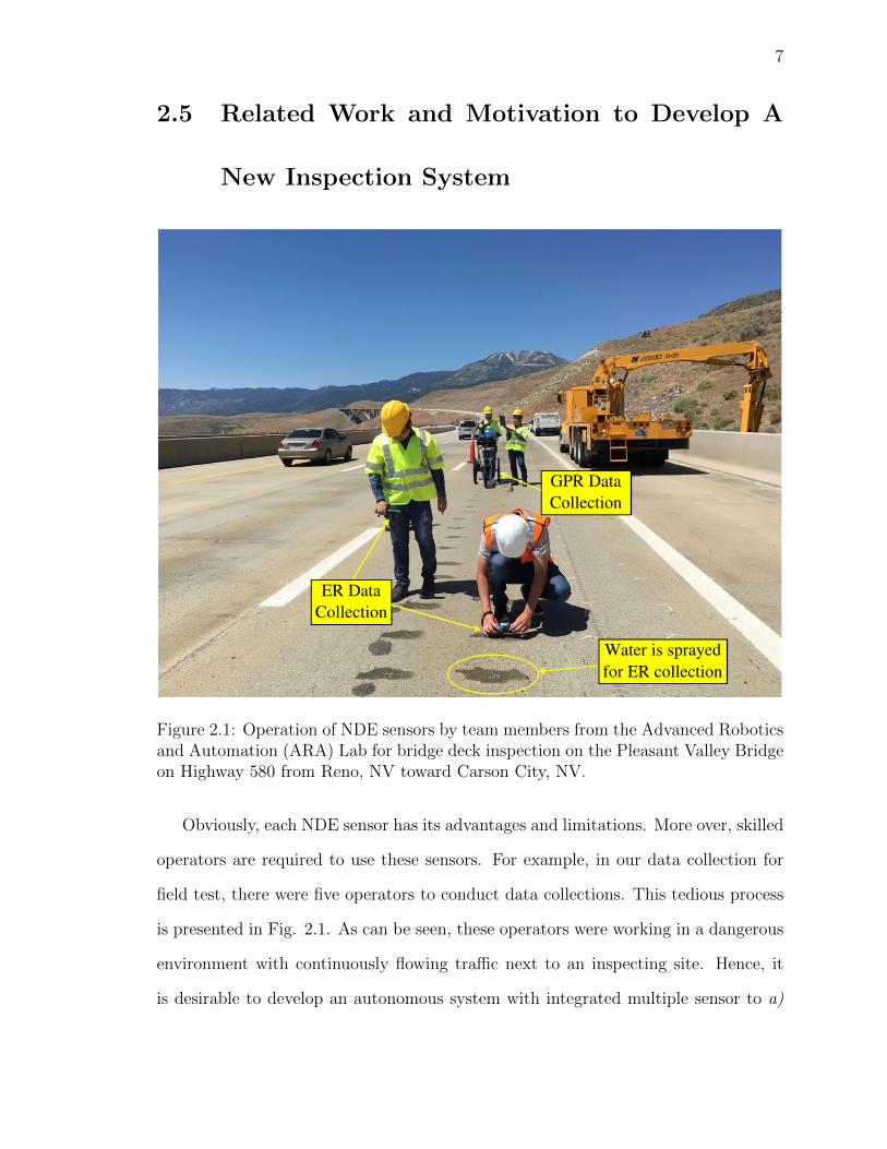
The camera-IMU calibration process was carried out followed the descriptions in

[75–77]. In this work, the Kalibr package [78] was utilized to automate the calibration

34

Figure 5.4: GPS-based localization with EKF. The robot has been driven along a 34ft-by14 ft square 10 times. The red plus sign denotes GPS location. The blue dotdenotes robot’s location from wheelodometry. The green dot denotes the localizationalgorithm’s output.

process. The calibration results are presented as follows. The extrinsic transformation

35

from left camera frame to IMU frame is:

0.99994075 0.00259196 0.0105729 −0.07692214

−0.01063558 0.02549736 0.99961831 0.01076284

0.00232139 −0.99967153 0.02552342 −0.02766903

0 0 0 1

(5.1)

The extrinsic transformation from right camera frame to IMU frame is:

0.99999025 0.00278813 0.00342473 0.04309024

−0.00349755 0.02654717 0.99964144 0.01090429

0.002692621 −0.99964367 0.02655666 −0.02746205

0 0 0 1

(5.2)

The extrinsic transformation from left camera to right camera is:

0.99997445 −0.0019256 0.0071454 −0.12001128

0.00018505 0.99999943 0.00105219 −0.00013146

−0.0071456 −0.00105084 0.99997392 −0.00055791

0 0 0 1

(5.3)

5.4 Robot deployment and Elevation map inside a

garage building

The robot has been deployed inside a garage building. Using AsusXtion RGBD

camera, the robot uses algorithms discussed in Section 4.3 to build an elevation map.

The results are presented below.

36

Figure 5.5: Static calibration result for left camera.

37

Figure 5.6: Static calibration result for right camera.

38

Figure 5.7: Acceleration error from IMU.

39

Figure 5.8: Angular velocity error from IMU.

Figure 5.9: Feature tracking performance from stereo visual inertial sensor.

40

Figure 5.10: The robot is moving inside a garage building.

Figure 5.11: Elevation map inside the garage parking. A car appears in front of therobot and the map is being updated accordingly.

41

Figure 5.12: Elevation map is being built when the robot moves along.

42

Chapter 6

Conclusions and Future Work

6.1 Conclusions

This thesis presented a robotic system for civil infrastructure inspection. The system

was designed and implemented with focusing on multiple sensors fusion, including

nondestructive evaluation sensors, GPS, cameras, IMU. Detailed discussion about

each sensor was provided. Several techniques for localization were provided with

emphasizing on complementaries among sensors. Some experimental results were

presented.

6.2 Future Work

Future work may include exhaustive field tests to evaluate the robot performance.

It is desirable to combine information from NDE sensors with navigation sensors to

generate intelligent inspection plans. One possible approach is: the robot first relies

on visual data to perform inspection. While reading data from the GPR sensor, the

43

robot might decide to deploy ER sensor at some specific locations, where GPR shows

bad data reading, which may indicate high level of deterioration. This approach

might reduce the total inspection time by performing deep inspection only where

it is needed. Additionally, several inspection robot could be employed to form a

multi-robot inspection network to quickly cover any vast area [79,80].

44

Bibliography

[1] T. P. Keane, “The economic importance of the national highway system,” Public

Roads, vol. 59, no. 4, 1996.

[2] D. of Transportation, “Making critical investments in highways and bridges.”

[Online]. Available: https://www.transportation.gov/sites/dot.gov/files/docs/

Making Critical Investments in Highway and Bridge Infrastructure.pdf

[3] “Highway bridges by wearing surface 2015,” US Department of Transportation,

Federal Highway Administration. [Online]. Available: https://www.fhwa.dot.

gov/bridge/nbi/no10/wearing15.cfm

[4] “Collapse of i-35w highway bridge minneapolis, minnesota,” National

Transportation Safety Board, August 1, 2007. [Online]. Available: http:

//www.dot.state.mn.us/i35wbridge/pdf/ntsb-report.pdf

[5] J. Wang, G. Li, R. Jiang, and Y. Chen, “Real-time monitoring of the bridge

cable health by acoustic emission and b-value analysis,” in Image and Signal

Processing (CISP), 2013 6th International Congress on, vol. 03, Dec 2013, pp.

1340–1345.

[6] M. Solla, R. Asorey-Cacheda, X. Nez-Nieto, and B. Riveiro, “Combined ap-

proach of gpr and thermographic data through fdtd simulation to analyze ma-

45

sonry bridges: The evaluation of construction materials in a restored masonry

arch bridge,” in Advanced Ground Penetrating Radar (IWAGPR), 2015 8th In-

ternational Workshop on, July 2015, pp. 1–4.

[7] M. Shigeishi, S. Colombo, K. Broughton, H. Rutledge, A. Batchelor, and

M. Forde, “Acoustic emission to assess and monitor the integrity of bridges,”

Construction and building materials, vol. 15, no. 1, pp. 35–49, 2001.

[8] R. F. Stratfull, “Experimental cathodic protection of a bridge deck,” Transporta-

tion Research Record, vol. 500, pp. 1–15, 1974.

[9] H. M. La, R. S. Lim, B. B. Basily, N. Gucunski, J. Yi, A. Maher, F. A. Romero,

and H. Parvardeh, “Mechatronic systems design for an autonomous robotic sys-

tem for high-efficiency bridge deck inspection and evaluation,” IEEE/ASME

Transactions on Mechatronics, vol. 18, no. 6, pp. 1655–1664, 2013.

[10] D. Huston, J. Cui, D. Burns, and D. Hurley, “Concrete bridge deck condition as-

sessment with automated multisensor techniques,” Structure and Infrastructure

Engineering, vol. 7, no. 7-8, pp. 613–623, 2011.

[11] N. Gucunski, S. Kee, H. La, B. Basily, A. Maher, and H. Ghasemi, “Implemen-

tation of a fully autonomous platform for assessment of concrete bridge decks

rabit,” in Structures Congress 2015, 2015, pp. 23–25.

[12] N. Gucunski, A. Maher, B. Basily, H. La, R. Lim, H. Parvardeh, and S. Kee,

“Robotic platform rabit for condition assessment of concrete bridge decks using

multiple nde technologies,” HDKBR INFO Magazin, vol. 3, no. 4, pp. 5–12, 2013.

[13] N. Gucunski, S.-H. Kee, H. La, B. Basily, and A. Maher, “Delamination and

concrete quality assessment of concrete bridge decks using a fully autonomous

46

rabit platform,” Structural Monitoring and Maintenance, vol. 2, no. 1, pp. 19–34,

2015.

[14] H. M. La, N. Gucunski, S.-H. Kee, J. Yi, T. Senlet, and L. Nguyen, “Autonomous

robotic system for bridge deck data collection and analysis,” in 2014 IEEE/RSJ

International Conference on Intelligent Robots and Systems. IEEE, 2014, pp.

1950–1955.

[15] K. Dinh, N. Gucunski, J. Kim, T. H. Duong, and H. M. La, “Attenuation-based

methodology for condition assessment of concrete bridge decks using gpr,” in

ISARC. Proceedings of the International Symposium on Automation and Robotics

in Construction, vol. 32. Vilnius Gediminas Technical University, Department

of Construction Economics & Property, 2015, p. 1.

[16] N. Gucunski, B. Basily, S.-H. Kee, H. La, H. Parvardeh, A. Maher, and

H. Ghasemi, “Multi nde technology condition assessment of concrete bridge

decks by rabittm platform,” in NDE/NDT for Structural Materials Technology

for Highway & Bridges, 2014, pp. 161–168.

[17] H. M. La, N. Gucunski, S.-H. Kee, and L. Nguyen, “Visual and acoustic data

analysis for the bridge deck inspection robotic system,” in ISARC. Proceedings

of the International Symposium on Automation and Robotics in Construction,

vol. 31. Vilnius Gediminas Technical University, Department of Construction

Economics & Property, 2014, p. 1.

[18] T. H. Johnsen, M. R. Geiker, and M. H. Faber, “Quantifying condition indicators

for concrete structures,” Concrete international, vol. 25, no. 12, pp. 47–54, 2003.

47

[19] B. Assouli, G. Ballivy, and P. Rivard, “Influence of environmental parameters

on application of standard astm c876-91: half cell potential measurements,”

Corrosion Engineering, Science and Technology, vol. 43, no. 1, pp. 93–96, 2008.

[20] S. Nazarian, M. R. Baker, and K. Crain, “Movable seismic pavement analyzer,”

Mar. 25 1997, uS Patent 5,614,670.

[21] R. D. Browne, “Mechanisms of corrosion of steel in concrete in relation to design,

inspection, and repair of offshore and coastal structures,” Special Publication,

vol. 65, pp. 169–204, 1980.

[22] A. Alongi, T. Cantor, C. Kneeter, and A. Alongi Jr, “Concrete evaluation by

radar theoretical analysis,” Transportation Research Record, no. 853, 1982.

[23] S. Cardimona, B. Willeford, J. Wenzlick, and N. Anderson, “Investigation of

bridge decks utilizing ground penetrating radar,” in International conference on

the application of geophysical technologies to planning, design, construction and

maintenance of transportation facilities. St. Louis/USA, 2000.

[24] Z. W. Wang, M. Zhou, G. G. Slabaugh, J. Zhai, and T. Fang, “Automatic

detection of bridge deck condition from ground penetrating radar images,” IEEE

Transactions on Automation Science and Engineering, vol. 8, no. 3, pp. 633–640,

July 2011.

[25] S. Nazarian, M. R. Baker, and K. Crain, “Development and testing of a seismic

pavement analyzer,” Tech. Rep., 1993.

[26] N. C. Davidson and S. B. Chase, “Initial testing of advanced ground-penetrating

radar technology for the inspection of bridge decks: the hermes and peres bridge

inspectors,” pp. 180–185, 1999.

48

[27] M. Scott, A. Rezaizadeh, and M. Moore, “Phenomenology study of hermes

ground-penetrating radar technology for detection and identification of common

bridge deck features,” Tech. Rep., 2001.

[28] N. Gucunski and A. Maher, “Bridge deck evaluation using portable seismic pave-

ment analyzer (pspa),” Tech. Rep., 2000.

[29] “Revolutionary rabit bridge deck assessment tool,” Center for Advanced

Infrastructure and Transportation, Rutgers University, 2014. [Online]. Available:

http://cait.rutgers.edu/rabit-asce-award

[30] M. J. Harry, “Ground penetrating radar theory and applications,” 2009.

[31] “Zed ros wrapper,” 2016. [Online]. Available: https://github.com/stereolabs/

zed-ros-wrapper

[32] J. Garcia and Z. Zalevsky, “Range mapping using speckle decorrelation,”

Sep. 20 2007, uS Patent App. 11/712,932. [Online]. Available: https:

//www.google.com/patents/US20070216894

[33] J. J. L. C. Stachniss and S. Thrun, “Simultaneous localization and mapping,” in

Springer handbook of robotics, B. Siciliano and O. Khatib, Eds. Springer, 2016,

ch. 46, pp. 1153–1171.

[34] J. Farrell and M. Barth, The global positioning system and inertial navigation.

McGraw-Hill Professional, 1999.

[35] M. S. Grewal, L. R. Weill, and A. P. Andrews, Global positioning systems, inertial

navigation, and integration. John Wiley & Sons, 2007.

[36] P. Misra and P. Enge, “Global positioning system: Signals, measurements and

performance second edition,” Massachusetts: Ganga-Jamuna Press, 2006.

49

[37] T. Moore, “robot localization,” 2014. [Online]. Available: http://wiki.ros.org/

robot localization

[38] D. Simon, Optimal state estimation: Kalman, H infinity, and nonlinear ap-

proaches. John Wiley & Sons, 2006.

[39] D. Alspach, “A parallel filtering algorithm for linear systems with unknown time

varying noise statistics,” IEEE Transactions on Automatic Control, vol. 19, no. 5,

pp. 552–556, Oct 1974.

[40] R. Kashyap, “Maximum likelihood identification of stochastic linear systems,”

IEEE Transactions on Automatic Control, vol. 15, no. 1, pp. 25–34, Feb 1970.

[41] K. Myers and B. Tapley, “Adaptive sequential estimation with unknown noise

statistics,” IEEE Transactions on Automatic Control, vol. 21, no. 4, pp. 520–523,

Aug 1976.

[42] B. Carew and P. Belanger, “Identification of optimum filter steady-state gain

for systems with unknown noise covariances,” IEEE Transactions on Automatic

Control, vol. 18, no. 6, pp. 582–587, Dec 1973.

[43] R. Mehra, “On the identification of variances and adaptive kalman filtering,”

IEEE Transactions on Automatic Control, vol. 15, no. 2, pp. 175–184, Apr 1970.

[44] ——, “Approaches to adaptive filtering,” IEEE Transactions on Automatic Con-

trol, vol. 17, no. 5, pp. 693–698, Oct 1972.

[45] B. J. Odelson, M. R. Rajamani, and J. B. Rawlings, “A new autocovariance least-

squares method for estimating noise covariances,” Automatica, vol. 42, no. 2, pp.

303–308, 2006.

50

[46] D. Titterton and J. L. Weston, Strapdown inertial navigation technology. IET,

2004, vol. 17.

[47] H. C. LEFERE, “Fundamentals of the interferometric fiber-optic gyroscope,”

Optical review, vol. 4, no. 1A, pp. 20–27, 1997.

[48] E. J. Post, “Sagnac effect,” Reviews of Modern Physics, vol. 39, no. 2, p. 475,

1967.

[49] H. Jin, P. Favaro, and S. Soatto, “Real-time 3d motion and structure of point

features: a front-end system for vision-based control and interaction,” in Com-

puter Vision and Pattern Recognition, 2000. Proceedings. IEEE Conference on,

vol. 2. IEEE, 2000, pp. 778–779.

[50] D. Nister, “Preemptive ransac for live structure and motion estimation,” Machine

Vision and Applications, vol. 16, no. 5, pp. 321–329, 2005.

[51] A. Chiuso, P. Favaro, H. Jin, and S. Soatto, “Structure from motion causally

integrated over time,” IEEE transactions on pattern analysis and machine intel-

ligence, vol. 24, no. 4, pp. 523–535, 2002.

[52] R. Yang and M. Pollefeys, “Multi-resolution real-time stereo on commodity

graphics hardware,” in Computer Vision and Pattern Recognition, 2003. Pro-

ceedings. 2003 IEEE Computer Society Conference on, vol. 1. IEEE, 2003, pp.

I–I.

[53] M. Nuttin, T. Tuytelaars, and L. Van Gool, “Omnidirectional vision based topo-

logical navigation,” International Journal of Computer Vision, vol. 74, no. 3, pp.

219–236, 2007.

51

[54] E. Eade and T. Drummond, “Scalable monocular slam,” in Proceedings of the

2006 IEEE Computer Society Conference on Computer Vision and Pattern

Recognition-Volume 1. IEEE Computer Society, 2006, pp. 469–476.

[55] G. Klein and D. Murray, “Parallel tracking and mapping for small ar

workspaces,” in Mixed and Augmented Reality, 2007. ISMAR 2007. 6th IEEE

and ACM International Symposium on. IEEE, 2007, pp. 225–234.

[56] A. J. Davison, “Real-time simultaneous localisation and mapping with a single

camera.” in ICCV, vol. 3, 2003, pp. 1403–1410.

[57] E. D. Dickmanns and B. D. Mysliwetz, “Recursive 3-d road and relative ego-state

recognition,” IEEE Transactions on pattern analysis and machine intelligence,

vol. 14, no. 2, pp. 199–213, 1992.

[58] G. Qian, R. Chellappa, and Q. Zheng, “Robust structure from motion estimation

using inertial data,” JOSA A, vol. 18, no. 12, pp. 2982–2997, 2001.

[59] S. I. Roumeliotis, A. E. Johnson, and J. F. Montgomery, “Augmenting inertial

navigation with image-based motion estimation,” in Robotics and Automation,

2002. Proceedings. ICRA’02. IEEE International Conference on, vol. 4. IEEE,

2002, pp. 4326–4333.

[60] D. Strelow and S. Singh, “Optimal motion estimation from visual and inertial

measurements,” in Applications of Computer Vision, 2002.(WACV 2002). Pro-

ceedings. Sixth IEEE Workshop on. IEEE, 2002, pp. 314–319.

[61] H. Rehbinder and B. K. Ghosh, “Pose estimation using line-based dynamic vision

and inertial sensors,” IEEE Transactions on Automatic Control, vol. 48, no. 2,

pp. 186–199, 2003.

52

[62] P. Gemeiner, P. Einramhof, and M. Vincze, “Simultaneous motion and structure

estimation by fusion of inertial and vision data,” The International Journal of

Robotics Research, vol. 26, no. 6, pp. 591–605, 2007.

[63] M. M. Veth and J. Raquet, “Fusing low-cost image and inertial sensors for passive

navigation,” Navigation, vol. 54, no. 1, pp. 11–20, 2007.

[64] A. I. Mourikis, N. Trawny, S. I. Roumeliotis, A. E. Johnson, A. Ansar, and

L. Matthies, “Vision-aided inertial navigation for spacecraft entry, descent, and

landing,” IEEE Transactions on Robotics, vol. 25, no. 2, pp. 264–280, 2009.

[65] M. Bloesch, S. Omari, M. Hutter, and R. Siegwart, “Robust visual inertial

odometry using a direct ekf-based approach,” in Intelligent Robots and Systems

(IROS), 2015 IEEE/RSJ International Conference on. IEEE, 2015, pp. 298–

304.

[66] E. S. Jones and S. Soatto, “Visual-inertial navigation, mapping and localization:

A scalable real-time causal approach,” The International Journal of Robotics

Research, vol. 30, no. 4, pp. 407–430, 2011.

[67] J. Kelly and G. S. Sukhatme, “Visual-inertial sensor fusion: Localization, map-

ping and sensor-to-sensor self-calibration,” The International Journal of Robotics

Research, vol. 30, no. 1, pp. 56–79, 2011.

[68] C. Hertzberg, R. Wagner, U. Frese, and L. Schroder, “Integrating generic sen-

sor fusion algorithms with sound state representations through encapsulation of

manifolds,” Information Fusion, vol. 14, no. 1, pp. 57–77, 2013.

[69] M. Herbert, C. Caillas, E. Krotkov, I.-S. Kweon, and T. Kanade, “Terrain map-

ping for a roving planetary explorer,” in Robotics and Automation, 1989. Pro-

ceedings., 1989 IEEE International Conference on. IEEE, 1989, pp. 997–1002.

53

[70] L. B. Cremean and R. M. Murray, “Uncertainty-based sensor fusion of range

data for real-time digital elevation mapping (rtdem),” in Proceedings of the IEEE

International Conference on Robotics and Automation, 2005, pp. 18–22.

[71] D. Belter, P. Labcki, and P. Skrzypczynski, “Estimating terrain elevation maps

from sparse and uncertain multi-sensor data,” in Robotics and Biomimetics (RO-

BIO), 2012 IEEE International Conference on. IEEE, 2012, pp. 715–722.

[72] P. Fankhauser, M. Bloesch, C. Gehring, M. Hutter, and R. Siegwart, “Robot-

centric elevation mapping with uncertainty estimates,” in International Confer-

ence on Climbing and Walking Robots (CLAWAR), 2014.

[73] I. S. Kweon and T. Kanade, “Extracting topographic terrain features from ele-

vation maps,” CVGIP: image understanding, vol. 59, no. 2, pp. 171–182, 1994.

[74] A. Kleiner and C. Dornhege, “Real-time localization and elevation mapping

within urban search and rescue scenarios,” Journal of Field Robotics, vol. 24,

no. 8-9, pp. 723–745, 2007.

[75] P. Furgale, J. Rehder, and R. Siegwart, “Unified temporal and spatial calibra-

tion for multi-sensor systems,” in Intelligent Robots and Systems (IROS), 2013

IEEE/RSJ International Conference on. IEEE, 2013, pp. 1280–1286.

[76] P. Furgale, T. D. Barfoot, and G. Sibley, “Continuous-time batch estimation

using temporal basis functions,” in Robotics and Automation (ICRA), 2012 IEEE

International Conference on. IEEE, 2012, pp. 2088–2095.

[77] J. Maye, P. Furgale, and R. Siegwart, “Self-supervised calibration for robotic

systems,” in Intelligent Vehicles Symposium (IV), 2013 IEEE. IEEE, 2013, pp.

473–480.

54

[78] “Kalibr,” 2014. [Online]. Available: https://github.com/ethz-asl/kalibr

[79] H. M. La and W. Sheng, “Distributed sensor fusion for scalar field mapping using

mobile sensor networks,” IEEE Transactions on cybernetics, vol. 43, no. 2, pp.

766–778, 2013.

[80] H. M. La, W. Sheng, and J. Chen, “Cooperative and active sensing in mobile

sensor networks for scalar field mapping,” IEEE Transactions on Systems, Man,

and Cybernetics: Systems, vol. 45, no. 1, pp. 1–12, 2015.