Santa Clara UniversityScholar Commons

Mechanical Engineering Master's Theses Engineering Master's Theses

2-2017

A Molecular Dynamics Study of Self-DiffusionAlong a Screw Dislocaton Core in Face-CenteredCubic CrystalsSiavash SoltanibajestaniSanta Clara Univeristy

Follow this and additional works at: http://scholarcommons.scu.edu/mech_mstr

Part of the Mechanical Engineering Commons

This Thesis is brought to you for free and open access by the Engineering Master's Theses at Scholar Commons. It has been accepted for inclusion inMechanical Engineering Master's Theses by an authorized administrator of Scholar Commons. For more information, please contactrscroggin@scu.edu.

Recommended CitationSoltanibajestani, Siavash, "A Molecular Dynamics Study of Self-Diffusion Along a Screw Dislocaton Core in Face-Centered CubicCrystals" (2017). Mechanical Engineering Master's Theses. 9.http://scholarcommons.scu.edu/mech_mstr/9

A MOLECULAR DYNAMICS STUDY OF SELF-DIFFUSION

ALONG A SCREW DISLOCATON CORE IN FACE-CENTERED

CUBIC CRYSTALS

By

Siavash Soltanibajestani

MASTER THESIS

Submitted in Partial Fulfillment of the Requirements

For the Degree of Master of Science

in Mechanical Engineering at

Santa Clara University, Feb 2017

Santa Clara, California

iii

To my wife Elahe and my mother Mahasti

for their support.

iv

AKNOWLEDGMENTS

I would like to thank my adviser Professor Sepehrband, for her support and encouragement when

times were tough. Without her knowledge and patient instructions, it was impossible to complete

this study. I would also like to express my gratitude to Professor Abdolrahim from University of

Rochester for being on the dissertation committee and her constructive comments.

This work was supported by Santa Clara University, School of Engineering. Resources for fast

computing were provided by the Center for Integrated Research Computing (CIRC) at University

of Rochester.

v

TABLE OF CONTENTS

LIST OF TABLES ................................................................................................................... vii

LIST OF FIGURES ................................................................................................................ viii

NOMENCLATURE .................................................................................................................. xi

ABSTRACT ............................................................................................................................ xii

CHAPTER 1 : INTRODUCTION .................................................................................................. 1

CHAPTER 2 : BACKGROUND AND OBJECTIVES .................................................................. 3

2.1 Molecular Dynamics (MD) ................................................................................................... 3

2.1.1 Interaction of atoms ........................................................................................................ 3

2.1.2 Newton’s Equations of Motion....................................................................................... 4

2.1.3 Boundary Conditions ...................................................................................................... 6

2.1.4 Time averaging of properties .......................................................................................... 8

2.1.5 Ensembles and Extended Systems .................................................................................. 9

2.1.6 Nose–Hoover Thermostat ............................................................................................... 9

2.2 Tools and visualization........................................................................................................ 10

2.2.1 LAMMPS ..................................................................................................................... 10

2.2.2 Visualization of defects ................................................................................................ 10

2.2.3 OVITO .......................................................................................................................... 13

2.3 Diffusion in solids ............................................................................................................... 14

2.4 Dislocation diffusion ........................................................................................................... 16

2.4.1 Formalism ..................................................................................................................... 16

2.4.2 Experimental measurements ......................................................................................... 17

2.4.3 Simulation Studies ........................................................................................................ 18

vi

2.4.4 Mechanisms of pipe-diffusion ...................................................................................... 18

2.5 Motivation ........................................................................................................................... 20

CHAPTER 3 : SIMULATION PROCESS ................................................................................... 21

3.1 Simulation set up ................................................................................................................. 21

CHAPTER 4 : RESULTS AND DISSCUSSION ........................................................................ 26

4.1 Activation energy of pipe diffusion .................................................................................... 26

4.2 Vacancy formation energy .................................................................................................. 37

4.3 Contribution of vacancy mechanism to diffusion along a screw dislocation core .............. 38

4.4 Conclusion ........................................................................................................................... 41

4.5 Future work ......................................................................................................................... 41

References ..................................................................................................................................... 43

Appendix A: Dislocation diffusivities .......................................................................................... 47

Appendix B: Sample script in LAMMPS ..................................................................................... 48

vii

List of Tables

Table 2.1: CNA signatures of common crystal structures [19] ................................................... 11

Table 4.1:Calculated separation distance of dislocations (d), pipe-diffusion activation energy

(Ed), integrated diffusion flux (P0) and pre-exponential factor of pipe-diffusion (D0). Stacking

fault energies (Estk_flt) and bulk diffusion activation energies (Eb) .......................................... 32

Table 2.1 is reproduced without permission.

viii

List of Figures

Figure 2.1: Steps of molecular dynamics simulation [14] ............................................................. 3

Figure 2.2: Periodic boundary conditions. The central cell is repeated in all directions [12] ...... 7

Figure 2.3 CNA group of FCC strucuture [33] ........................................................................... 12

Figure 2.4: Schematic illustration of the DXA [32] .................................................................... 13

Figure 2.5: (a) The atomic configuration; (b) the stress field, where red shows the tensile and

blue indicates the compressive region; right: the barriers for diffusion in the compressive (1) and

tensile (2) regions in the vicinity of partial dislocation cores and in the stacking fault ribbon (3)

[46]. ……………………………………………………………………………………………..19

Figure 3.1: A screw dislocation along axis of a cylinder of radius R and Burgers vector b [52]. 22

Figure 3.2: A slice parallel to dislocation line shown with red segment. Green atoms represent

atoms in perfect FCC structure. .................................................................................................... 23

Figure 3.3: Relaxation of a system containing a screw dislocation in Al. (a) Initial structure with

the dislocation core at the center of the cylinder. Atoms in core regions have higher potential

energy (b) the relaxed structure (c) the potential energy of the system decreases during

relaxation to bring the system to equilibrium state ....................................................................... 24

Figure 3.4: Relaxed structures of the dislocation in (a) Al, (b) Ni, (c) Cu and (d) Ag. A slice of

the simulation box parallel to the dislocation line is shown. Green and red atoms represent FCC

and HCP structures (stacking fault) respectively. Blue segments show partial dislocations. ...... 25

Figure 4.1: Total energy vs. time in Al during 1ns of NVE ensemble at 1000 K. ....................... 26

Figure 4.2: A slice of cylinder parallel to the dislocation line (a) Al at 900 K (0.86Tm), Ni at

1550 K (0.9 Tm), (c) Cu at 1300 K (0.98 Tm) and (c) Ag at 1150 K (0.9 Tm). Atoms are color

coded using the absolute displacements along the dislocation core after 30 ns of isothermal

annealing. The dislocation core is at the center of the cylinder. ................................................... 27

Figures 2.1 to 2.5 are reproduced without permission.

ix

Figure 4.3: Top view of the simulation cell. Imaginary cylinders with different radii ranging from

5Å to 13Å, centered at midpoint between partials are chosen. ..................................................... 28

Figure 4.4: Mean squared displacements along the core of a screw dislocation in (a) Al at T=900

K, (b) Cu at T=1300 K and (c) at T=1550K for Ni. The displacements are shown for different

values of radius, R......................................................................................................................... 29

Figure 4.5: Average diffusivity vs. R for (a) Al (b) Cu and (c) Ni. .............................................. 30

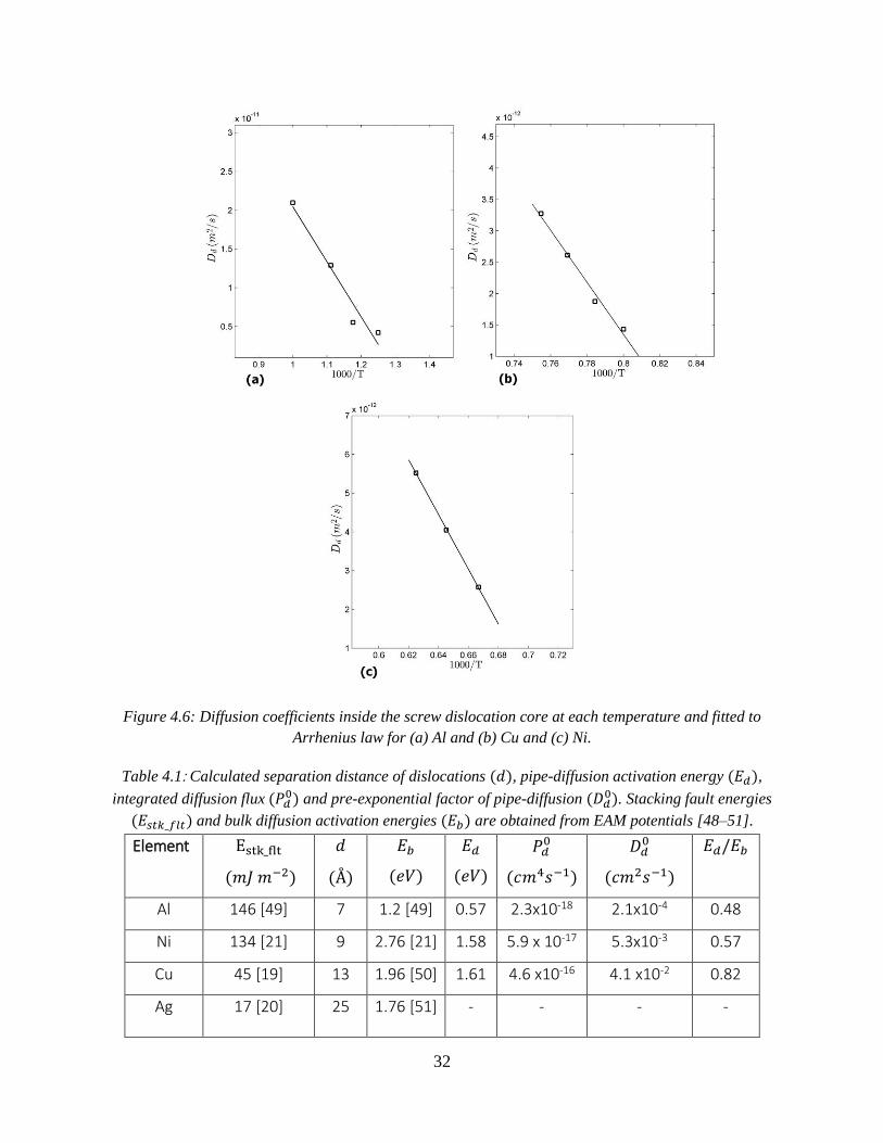
Figure 4.6: Diffusion coefficients inside the screw dislocation core at each temperature and fitted

to Arrhenius law for (a) Al and (b) Cu and (c) Ni. ....................................................................... 32

Figure 4.7: diffusion of atoms along the dislocation line in Al at 900 K after 30 ns in a cylinder

with R= 13 Å. The unwrapped coordinates of atoms are shown. ................................................. 34

Figure 4.8: A slice of cylinder parallel to dislocation line and configuration of partial dislocations

at a random snapshot for (a) Al at 900 K (0.86Tm) (b) Ni at 1550 K (0.90 Tm), (c) Cu at 1300 K

(0.98 Tm) and (d) Ag at 1150 K (0.9 Tm). .................................................................................... 35

Figure 4.9 Wigner-Seitz defect analysis: (a) formation of a vacancy-interstitial (b) these two

point defect briefly separate and migrate along the core (c) vacancy and interstitial recombine (d)

formation of vacancy-interstitial pair in core regions at high temperatures ................................. 36

Figure 4.10: Vacancy formation energy in the vicinity of the partial dislocations (green colored

circles) in copper. .......................................................................................................................... 37

Figure 4.11: Average diffusivity vs. R with a single vacancy and a screw dislocation in the

system in Cu. ................................................................................................................................. 38

Figure 4.12: Diffusion coefficients inside the screw dislocation core at each temperature without

any pre-existing point defects (intrinsic) and in the presence of equilibrium number of vacancies

and a screw dislocation in Cu. ...................................................................................................... 40

x

Nomenclature

𝑁 number of atoms in the simulation box

𝑈 potential energy

𝐹𝑖 embedding energy of an atom in the local electron density

∅ electrostatic, two-atom interaction

𝑟𝑖 coordinates of atom i

𝑚 mass

𝑎 acceleration

𝑣 velocity

𝑡 time

𝐿 length of the simulation box

𝑁𝑡 number of time steps

𝐾 kinetic energy

𝑇 temperature

𝑘𝐵 Boltzman constant

𝐸 total energy of the system

𝑠 scaling factor parameter of time

𝜁 drag force parameter

𝐶𝑆𝑃 centrosymmetry parameter

𝑟cut cutoff distance

𝑎fcc lattice constant of an fcc structure

𝑐𝑖 modified centrosymmetry parameter

𝐷𝑘 number of nearest neighbors

𝑅𝑗 bond vector

𝑐𝐴 concentration of atom A

𝐷𝐴 diffusion coefficient of atom A

𝐷0 pre-exponential factor of diffusion coefficient

𝐸𝐴 activation energy of diffusion of atom A

xi

𝑙 length of diffusive jump

𝜏 time between atomic jumps

𝑛 number of atomic jumps

𝑃𝑑 integrated flux of pipe-diffusion

𝐴𝑑 cross-sectional area of dislocation core

𝐷𝑑 diffusion coefficient along dislocation core

𝐷𝑑0 pre-exponential factor of pipe-diffusion coefficient

𝐸𝑑 activation energy of self-pipe-diffusion

𝐸𝑏 activation energy of self-diffusion in bulk

𝐷eff effective diffusion coefficient

𝜌 dislocation density

𝑢𝑖 displacement of atom i

𝑏 Burgers vector

𝑀𝑆𝐷 Mean Squared Displacement

𝑟𝑑 radius of dislocation core

𝑒 Euler’s number

𝐸stk_flt stacking fault energy

𝑑 dissociation width of partial dislocations

𝐸𝑣𝑓 vacancy formation energy

𝑁𝑣 equilibrium number of vacancies

𝑅 radius

𝐷𝑑𝑣 contribution of vacancy mechanism to pipe-diffusion

𝐷𝑑𝐼 contribution of intrinsic mechanism to pipe-diffusion

xii

ABSTRACT

The topic of this research is self-diffusion along a 1 2⁄ ⟨110⟩ screw dislocation core in face-

centered cubic metals. Using molecular dynamics, self-diffusion along a screw dislocation core

in four FCC metals, aluminum, copper, nickel and silver is investigated. In all metals under study

except in Ag, the results show high diffusivity along the core even in the absence of any pre-

existing point defects (intrinsic diffusion). Enhanced self-diffusion due to screw dislocations is

more remarkable in Al and Ni than in Cu. This behavior has been related to the stacking fault

energy and dissociation width of partial dislocations.

The simulations show generation of point defects (e.g. vacancy and interstitial) in core

regions at high temperatures, which leads to high diffusivity along the core. Formation of point

defects is suggested to be due to reversion of partial dislocations into a full dislocation, where a

point defect forms and starts to migrate. The reversion of partials into a full dislocation is

observed to occur more frequently in Al and Ni, due to their higher stacking fault energy and

lower dissociation width compared to Cu.

Moreover, by introducing a single vacancy in the core regions of Cu, the vacancy

mechanism contribution to diffusion was measured and found to be negligible compared to the

contribution of intrinsic diffusion. This indicates that the dislocation core becomes an effective

source of point defect generation at high temperatures to an extent that the effect of pre-existing

point defects on diffusion becomes negligible.

1

CHAPTER 1: INTRODUCTION

Diffusion in solids is an important topic of solid state physics since it plays an important role in

many microstructural changes during heat treatment of materials. Examples of such diffusion-

controlled evolution include nucleation of new phases, phase transformations, precipitation and

dissolution of a second phase, homogenization of alloys, recrystallization and high-temperature

creep, surface hardening of steel, diffusion bonding and sintering [1].

Through experimental studies, it has been established that the presence of line defects (e.g.

dislocations) significantly enhances the diffusion rate in crystalline materials [2]. High

diffusivity paths provided by dislocation cores have been reported to enhance the kinetics of

materials processes such as creep [3], formation of solute chains along dislocations and diffusion

of alloying elements [4] and coarsening kinetics in precipitation strengthened alloys [5].

Experimental studies of diffusion along dislocation cores which is also referred to as “pipe-

diffusion”, are divided into two categories: direct methods and indirect methods. In direct

methods, the diffusion coefficient is measured from the concentration vs. depth profile of a

radioactive tracer diffused in a deformed single crystal or low-angle grain boundaries [2]. By

measuring the integrated diffusion flux, 𝑃𝑑, assuming that the dislocation lines are normal to the

surface and estimating the cross sectional area, 𝐴𝑑, of the dislocation pipe, it is possible to

extract the diffusion coefficient, 𝐷𝑑, using 𝑃𝑑 = 𝐷𝑑𝐴𝑑. In these studies, it is often assumed that

𝐴𝑑 = 𝜋𝑟𝑑2 is the cross sectional area of the dislocation pipe with 𝑟𝑑 = 5 Å [2,6]. In indirect

methods, 𝑃𝑑 is back-calculated from the rate of a specific diffusion-controlled process such as

dislocation climb [7]. Most of the experimental studies are based on crude approximations and

assumptions which limit our understanding of the phenomenon. In order to study pipe-diffusion

at the atomic scale, Computational Materials Science and Engineering (CMSE) is widely

employed [8–11].

CMSE is the computer-based employment of modeling and simulation to understand the

materials behavior. The Molecular Dynamics (MD) method is one of the most popular methods

of modeling in CMSE in order to study the structure and micro-structural changes of materials

[12].

2

Diffusion along the dislocation core in crystalline materials has been extensively studied

using MD [8–11,13]. MD studies of pipe-diffusion confirm the mobility of atoms is much

higher in core regions than surrounding lattice sites. These studies [8,10] are mainly based on

introducing a point defect, either a vacancy or interstitial in core regions and following the

migration path of the defect, assuming that the diffusion is only controlled by migration of these

point defects. Results associated with a lower formation and/or migration energy of point defects

in core regions were obtained, which indicate high diffusivity along the core. Moreover, Pun et.

al. [9], using an MD study of pipe-diffusion, showed that even in the absence of any pre-existing

point defects, the activation energy of pipe-diffusion is much lower than the activation energy of

self-diffusion in bulk. The existence of this intrinsic diffusion (e.g. the diffusion along the core in

the absence of any pre-existing point defects), has been established only in Al [9], a metal with

high stacking fault energy. Therefore, an interesting topic of study is to investigate the existence

of the intrinsic diffusion along the core in other crystalline materials with different stacking fault

energies.

The purpose of the present study is to study self-diffusion phenomenon along the

dislocation core using a MD simulation. The focus is on self-diffusion along a 1 2⁄ ⟨110⟩ screw

dislocation core in Face-Centered Cubic (FCC) metals. Since in FCC metals, the 1 2⁄ ⟨110⟩

dislocations tend to dissociate into partial dislocations and the dissociation width depends on the

stacking fault energy, four FCC metals with different stacking fault energies are selected. Pipe-

diffusion is studied without introducing any point defects in the structure. Activation energy of

self-diffusion along the dislocation core in each of these metals is calculated and compared to

activation energy of self-diffusion in bulk. Moreover, a discussion of the high-diffusivity

mechanism along the core is included.

3

CHAPTER 2: BACKGROUND AND OBJECTIVES

2.1 Molecular Dynamics (MD)

In general, molecular dynamics study involves a set of steps which can be organized into

Domain Construction, Equilibrium and Relaxation, Objective Run and Post Processing as shown

in Figure 2.1.

Figure 2.1: Steps of molecular dynamics simulation [14].

Domain Construction is a process where particles are generated and their positions are assigned.

This step includes arranging the particles in the system and most of the time atoms are organized

into a crystal structure according to the type of the material under study and its lattice. Once all

particles are assigned to their positions, the next process is to relax the system statically at 0 K to

bring the system to lowest energy state. The geometry of the structure is optimized by

minimizing the energy of the structure which is done by iteratively adjusting atomic coordinates

so that the final configuration of the structure is close to real material crystal. Equilibration then

takes place to bring the system into desired temperature and thermal conditions [14].

In Objective Run step, the domain is subjected to desired experiment conditions, such as

applied forces on the system or different thermal conditions. During this step, the data files

including positions of atoms along with other parameters and attributes such as velocities, forces

and stresses are generated and can be used for further analysis in post processing stage [14].

2.1.1 Interaction of atoms

In order to obtain the properties of a solid in MD, a description of the interactions and forces

between its constituent atoms is required. This can be achieved by solving the quantum

4

mechanics equations of all the nuclei and electrons in the system, which is extremely

computationally intensive. MD utilizes a less complicated approach which is based on simple

functional forms describing the types of bonding and interactions in solids. These functions are

approximations to real interactions and therefore any calculations based on them will also give

approximations of the materials properties [12]. The most fundamental quantity that defines the

energetics and thermodynamics of a material is its potential energy, which is the sum of the

energetic interactions between the atoms. In a system of 𝑁 atoms, the cohesive energy (e.g. the

potential energy of the material at 0 K), 𝑈, is the negative of the energy needed to move all

constituent atoms of the system infinitely far apart [12].

In Embedded-Atom Method (EAM), proposed by Daw and Baskes [15], 𝑈, is seen as the

energy obtained by embedding an atom into the local electron density of the remaining atoms of

the system. In addition there is an electrostatic interaction between atoms. Therefore [15]:

𝑈 = ∑ 𝐹𝑖𝑒[∑ 𝑓𝑖𝑗(𝑟𝑖𝑗)𝑗≠𝑖 ]𝑖 +

1

2 ∑ ∑ Ø𝑖𝑗(𝑟𝑖𝑗)𝑁

𝑗=1𝑁𝑖=1 Equation 2.1

where 𝐹𝑖𝑒 is the embedding energy, f is some function of the interatomic distance representing an

approximation of the electron density, and Ø is an electrostatic, two-atom interaction and rij is

the distance between atom i and j. It can be seen that Daw and Baskes [15] defined the

embedding energy as the interaction of the atom with the background electron gas. In this

approach, metallic bonding can be viewed as if each atom is embedded in a host electron gas

created by its neighboring atoms [16]. It is possible to obtain the functions in Equation 2.1

empirically by fitting to properties of the bulk metals. Given the potential energy of a system as a

function of the position of its particles, force on 𝑖𝑡ℎ atom can be found using [12]:

𝐹𝑖 = −∇𝑖𝑈(𝑟1, 𝑟2, … , 𝑟𝑁) = −∇𝑖𝑈(𝑟𝑁) Equation 2.2

where the gradient is taken with respect to the coordinates of atom 𝑖, 𝑟𝑖.

2.1.2 Newton’s Equations of Motion

To get consecutive configurations of the particles in an MD simulation, Newton’s equations of

motion are solved for all particles in the system [17]. The equilibrium properties of the system

5

are then calculated from the motions of the atoms. According to Newton’s second law of motion

[12]:

𝐹𝑖 = 𝑚𝑖𝑎𝑖 = 𝑚𝑖𝑑2𝑟𝑖

𝑑𝑡2 Equation 2.3

where 𝐹𝑖 is the force on ith particle and can be obtained from Equation 2.2 and empirical

potentials, m is the mass of the particle, a is acceleration and 𝑡 is time. In order to get trajectory

of atoms, numerical integration is carried out using finite difference method. The most

commonly used time integration algorithm is the Verlet algorithm [18,19]. In this method, time

is discretized and ∆t is normally chosen so as to be as small as the period of the fastest atomic

vibrations (≈ 10−15 𝑠). In this short time interval, the forces acting on the particles are simply

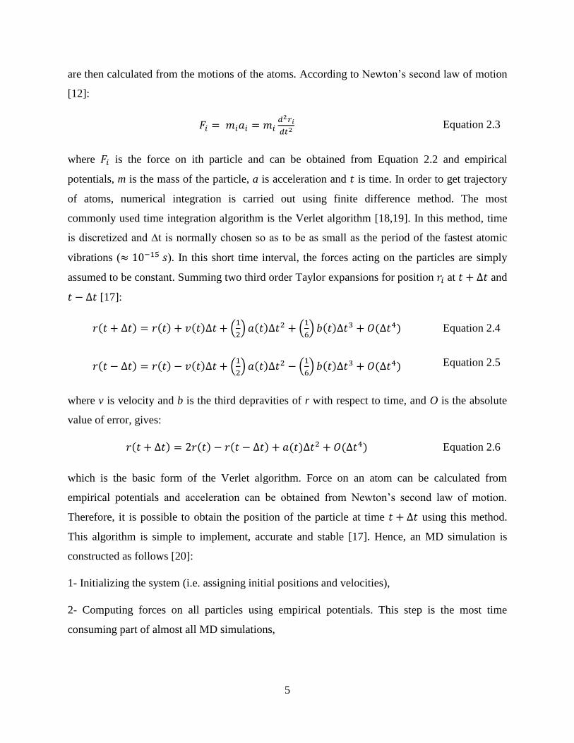
assumed to be constant. Summing two third order Taylor expansions for position 𝑟𝑖 at 𝑡 + ∆𝑡 and

𝑡 − ∆𝑡 [17]:

𝑟(𝑡 + Δ𝑡) = 𝑟(𝑡) + 𝑣(𝑡)Δ𝑡 + (1

2) 𝑎(𝑡)Δ𝑡2 + (

1

6) 𝑏(𝑡)Δ𝑡3 + 𝑂(Δ𝑡4) Equation 2.4

𝑟(𝑡 − Δ𝑡) = 𝑟(𝑡) − 𝑣(𝑡)Δ𝑡 + (1

2) 𝑎(𝑡)Δ𝑡2 − (

1

6) 𝑏(𝑡)Δ𝑡3 + 𝑂(Δ𝑡4) Equation 2.5

where v is velocity and b is the third depravities of r with respect to time, and O is the absolute

value of error, gives:

𝑟(𝑡 + Δ𝑡) = 2𝑟(𝑡) − 𝑟(𝑡 − Δ𝑡) + 𝑎(𝑡)Δ𝑡2 + 𝑂(Δ𝑡4) Equation 2.6

which is the basic form of the Verlet algorithm. Force on an atom can be calculated from

empirical potentials and acceleration can be obtained from Newton’s second law of motion.

Therefore, it is possible to obtain the position of the particle at time 𝑡 + ∆𝑡 using this method.

This algorithm is simple to implement, accurate and stable [17]. Hence, an MD simulation is

constructed as follows [20]:

1- Initializing the system (i.e. assigning initial positions and velocities),

2- Computing forces on all particles using empirical potentials. This step is the most time

consuming part of almost all MD simulations,

6

3- Integrating Newton’s equation of motion (using integration methods such as Verlet

algorithm). This step and previous one are repeated until reaching the desired length of time.

4- Deducing average quantities and global material properties after completion of the central

loop.

The trajectories simulated by MD should be sufficiently long to give meaningful samples

of the system configurations. Depending on the temperature and the characteristic of the system,

the number of MD steps required will differ. In general, simulations of solids should be longer

compared to liquids because of lower mobility of atoms in solids [21].

2.1.3 Boundary Conditions

The goal in most molecular dynamics simulation is to obtain physical properties of a

macroscopic system which can be greatly larger than system sizes that a computer can handle in

a reasonable amount of time [1]. For instance, a silver cube with volume 1 cm3 contains

approximately 5 × 1022 atoms, therefore to simulate some properties of this cube, to calculate 𝑎𝑖

and 𝑣𝑖 at each time step in 𝑥, 𝑦 and 𝑧 directions, 6𝑁 (𝑁 = number of atoms) difference

equations must be solved, which is almost impossible with computer resources we have today

[22].

Therefore, a method is needed to obtain realistic results using small system sizes. A

common method to solve this problem, is to use periodic boundary conditions. Using this

method, the system is viewed as an infinite array of equivalent finite systems. The atoms are

placed in a simulation cell which is then replicated throughout the space as shown in Figure 2.2

[12]. This periodicity has two consequences: the first is that if an atom exists the simulation cell,

it immediately reenters the cell from the opposite face. Secondly, atoms within a distance of 𝑟𝑐 of

boundary interact with the adjacent replica of the simulation cell, meaning, they interact with

atoms near the opposite boundary [23].

7

Figure 2.2: Periodic boundary conditions. The central cell is repeated in all directions. As a particle in

the central cell moves, its images move in the same way [12].

While integrating the equations of motions and interaction computation, the effect of the

periodic walls must be taken into account. After each time step, if an atom is found to have

moved outside the simulation box, its coordinates must be corrected to bring it back inside. For

example, if the x coordinate is defined to be between −𝐿𝑥

2 and

+𝐿𝑥

2, where 𝐿𝑥 is the simulation box

length in x direction, each atom must be tested using these equations:

If 𝑟𝑖𝑥 ≥𝐿𝑥

2, replace it by 𝑟𝑖𝑥 − 𝐿𝑥;

Otherwise, if 𝑟𝑖𝑥 <−𝐿𝑥

2, replace it by 𝑟𝑖𝑥 + 𝐿𝑥.

To calculate the interaction between particles in the system, the components of the distance

vector must be obtained by similar approach:

If 𝑟𝑖𝑗𝑥 ≥𝐿𝑥

2, replace it by 𝑟𝑖𝑗𝑥 − 𝐿𝑥;

Otherwise, if 𝑟𝑖𝑗𝑥 <−𝐿𝑥

2, replace it by 𝑟𝑖𝑗𝑥 + 𝐿𝑥.

The use of periodic boundary conditions confines the interaction range of each atom to no

more than half the smallest simulation box dimension, which is not an issue because the range of

interactions in EAM potentials is generally much less [23]. Even with periodic boundaries,

finite-size effects are still present. The proper size of the system to be able to neglect these

effects depends on the system and the properties of interest. As a minimal requirement, the size

8

should be larger than the rage of any interaction to ensure the periodicity is implemented

correctly [23].

2.1.4 Time averaging of properties

Using statistical mechanics and by performing time averages it is possible to relate the

microscopic behavior of the system to macroscopic properties. The properties of the system such

as temperature, pressure and internal energy are functions of coordinates and velocities of atoms.

Therefore one can find instantaneous value of a physical property, 𝐴(𝑡) at time t [17]:

𝐴(𝑡) = 𝑓(𝑟1(𝑡), … , 𝑟𝑁(𝑡), 𝑣1(𝑡), … , 𝑣𝑁(𝑡)) Equation 2.7

And then obtain its average:

⟨𝐴⟩ =1

𝑁𝑡∑ 𝐴(𝑡)

𝑁𝑡𝑡=1 Equation 2.8

where 𝑁𝑡 is the number of time steps and angled brackets denote time averaging. The most

commonly measured physical properties are discussed as follows.

Potential energy: The average potential energy, 𝑈, is obtained by averaging its instantaneous

value, which is usually obtained at the same time as the force computation is made using

empirical potentials. Even if not strictly necessary to perform the time integration knowledge of

𝑈 is required to verify energy conservation. This is an important check to do in any MD

simulation [17].

Kinetic energy: The instantaneous kinetic energy is given by [17]:

𝐾(𝑡) =1

2∑ 𝑚𝑖[𝑣𝑖(𝑡)]2

𝑖 Equation 2.9

Total energy: 𝐸 = 𝐾 + 𝑈 is a conserved quantity in Newtonian dynamics and it is common

to compute it at each time step to check the validity of the simulation. However, some fluctuation

in total energy is tolerated due to discretization of time integration; these errors can be reduced

by decreasing the time step, if needed [17].

9

Temperature: The temperature 𝑇 is directly related to the kinetic energy by the well-known

equipartition formula, assigning an average kinetic energy 𝑘𝐵𝑇 2⁄ per degree of freedom:

𝐾 =3

2𝑁𝑘𝐵𝑇 Equation 2.10

An estimate of the temperature can therefore be obtained from the average kinetic energy 𝐾 [17].

2.1.5 Ensembles and Extended Systems

In order to mimic various interactions (such as heat and mass exchange) of the surrounding

environment with the system, special coupling procedures, each of which corresponding to a

specific statistical ensemble in the language of statistical mechanics, can be used [24]. For

instance, MD simulations with fixed or periodic boundary conditions correspond to the micro-

canonical or NVE ensemble, where abbreviation NVE means that total number of particles N,

volume 𝑉 and total energy 𝐸 of the system are all conserved during the MD run [24,25].

Isothermal isobaric or NPT ensemble is achieved when a system interacts with an external

barostat and thermostat, so its temperature remains constant while the volume is adjusted to

control the pressure [20]. A straightforward approach to control the temperature is to scale the

atomic velocities during the simulation to reset the temperature to desired value. However, this

method disrupts the dynamic of atoms and results in artifacts in the simulation. A better approach

is to use Nose-Hoover thermostat to control the temperature [24].

2.1.6 Nose–Hoover Thermostat

Introducing a new dynamical variable, 𝑠, that serves as a scaling factor of time, Nose [26] was

able to mimic the interaction of a large reservoir that exchanges heat with the system. Although

this time scaling factor distorts Newton equation of motion, it enables us to keep the system

temperature to a desired value. The following equations of motion describe the evolution of the

system in the form suggested by Hoover [27]:

𝑑𝑟𝑖(𝑡)

𝑑𝑡= 𝑣𝑖(𝑡) Equation 2.11

10

𝑑𝑣𝑖(𝑡)

𝑑𝑡=

𝐹𝑖(𝑡)

𝑚− 𝜁(𝑡)𝑣𝑖(𝑡) Equation 2.12

𝑑𝜁(𝑡)

𝑑𝑡=

1

𝑀𝑠[∑ 𝑚|𝑣𝑖(𝑡)|2 − 3𝑁𝑘𝐵𝑇𝑁

𝑖=1 ] Equation 2.13

𝑑𝑠(𝑡)

𝑑𝑡= 𝑠(𝑡)𝜁(𝑡) Equation 2.14

where, 𝑀𝑠 is a thermal “mass” parameter that controls the rate of heat exchange. When the

kinetic energy exceeds (3/2)𝑁𝑘𝐵𝑇, i.e. when the instantaneous temperature exceeds the desired

temperature 𝑇, 𝜁 will increase. As soon as 𝜁 becomes positive, it exerts a viscous drag force on

all atoms, forcing them to reduce their velocities and lowering the instantaneous temperature.

Therefore, the temperature will fluctuate around a preselected value [24].

2.2 Tools and visualization

2.2.1 LAMMPS

LAMMPS [28] (Large-scale Atomic/Molecular Massively Parallel Simulator) is a classical

molecular dynamics code. It is developed by Sandia National Laboratories, USA and is designed

for MD simulations. LAMMPS has the capability to perform simulations on multiple processors

which results in decreasing the simulation time significantly.

The input code generated by the user defines the materials properties (such as crystal

structure) and the environment. The interaction of atoms is defined using potential files available

in literature or is defined by the user. The type of ensemble, time step (generally in the order of

femtoseconds), boundary conditions and the number of time steps are also defined by the user.

The output files (dump files) generally contain atom IDs and coordinates of atoms.

2.2.2 Visualization of defects

Since classical atomistic simulation models, such as MD, do not monitor crystal defects

explicitly, many computational analysis methods have been developed to enable the visualization

of the defects. Most of these methods are based on matching a local structure to an ideal one (e.g.

FCC or BCC) and quantifying how closely they match [29]. The most commonly used structure

11

characterization methods for MD simulations of crystalline solids are Common Neighbor

Analysis (CNA) [30], Centrosymmetry Parameter (CSP) [31] and Dislocation Extraction

Algorithm (DXA) [32].

2.2.2.1 Common neighbor analysis

Common neighbor analysis, CNA [30], can be applied to assign a crystal structure to an atom. In

this method, two atoms are assumed to be bonded if they are within a cut off distance, 𝑟cut,

which is set to be halfway between the first and second neighbor shell. For example, for FCC

structure, 𝑟𝑐𝑢𝑡 can be computed using [29]:

𝑟cutfcc =

1

2(√

1

2+ 1) 𝑎fcc ≈ 0.854 𝑎fcc Equation 2.15

where a is the lattice parameter. Three characteristic numbers are then calculated for each of the

N neighbor bonds of the central atom: The number of neighbor atoms the central atom and its

bonded neighbor have in common, 𝑛𝑐𝑛; the total number of bonds between these common

neighbors, 𝑛𝑏; and the number of bonds in the longest chain of bonds connecting the common

neighbors, 𝑛𝑙𝑐𝑏. This yields N triplets (𝑛𝑐𝑛, 𝑛𝑏 , 𝑛𝑙𝑐𝑏), which are compared to assign a structural

type to the central atom using Table 2.1 [29].

Table 2.1: Triplets in common crystal structures [29]

For example, in Figure 2.3, atom number 1 and its neighbor, atom number 2, have 4 neighbors in

common which are atoms number 3, 4, 5 and 6. Therefore 𝑛𝑐𝑛 for atom number 1 is 4. The total

number of bonds between these common neighbors is 2, as shown in the figure. Therefore 𝑛𝑏 is

2. The longest chain of bonds connecting the common neighbors is 1 (the bond number 1 or the

bond number 2). Therefore the triplet for atom number 1, an atom in perfect FCC structure, is

(421).

12

Figure 2.3: CNA group of FCC strucuture [33].

2.2.2.2 Centrosymmetry

The CentroSymmetry Parameter (CSP) can be used to quantify the local environment around an

atom. Each atom has equal number of equal and opposite nearest neighbor vectors and in the

undistorted case, the resultant of each pair of equal and opposite nearest neighbor vectors is

always zero, however, it is greater than zero in case there is a defect around. This parameter is

defined by [31]:

𝐶𝑆𝑃 = ∑ |𝑟𝑖 + 𝑟𝑖+𝑁/2|2𝑁/2𝑖=1 Equation 2.16

where 𝑟𝑖 and 𝑟𝑖+𝑁/2 are vectors from the central atom to a pair of opposite neighbors. The CSP

has the units of Å2 and is close to zero for regular sites of a centrosymmetric crystal and becomes

non-zero for defect atoms. The number of nearest neighbors taken into account is 𝑁 = 12 for

FCC and 𝑁 = 8 for bcc. A modified definition of CSP was proposed by Li [34] where CSP is

calculated by:

𝑐𝑖 =∑ 𝐷𝑘

𝑚𝑖/2

𝑘=1

∑ |𝑅𝑗|2𝑚𝑖𝑗

Equation 2.17

where 𝑐𝑖 is the central symmetry parameter of 𝑖th atom; 𝐷𝑘 = |𝑅𝑘 + 𝑅𝑘′ |2; 𝑚𝑖 is the number of

nearest neighbors; 𝑅𝑗 and 𝑅𝑘′ are the bond vectors. In this case central symmetry parameter is

dimensionless.

13

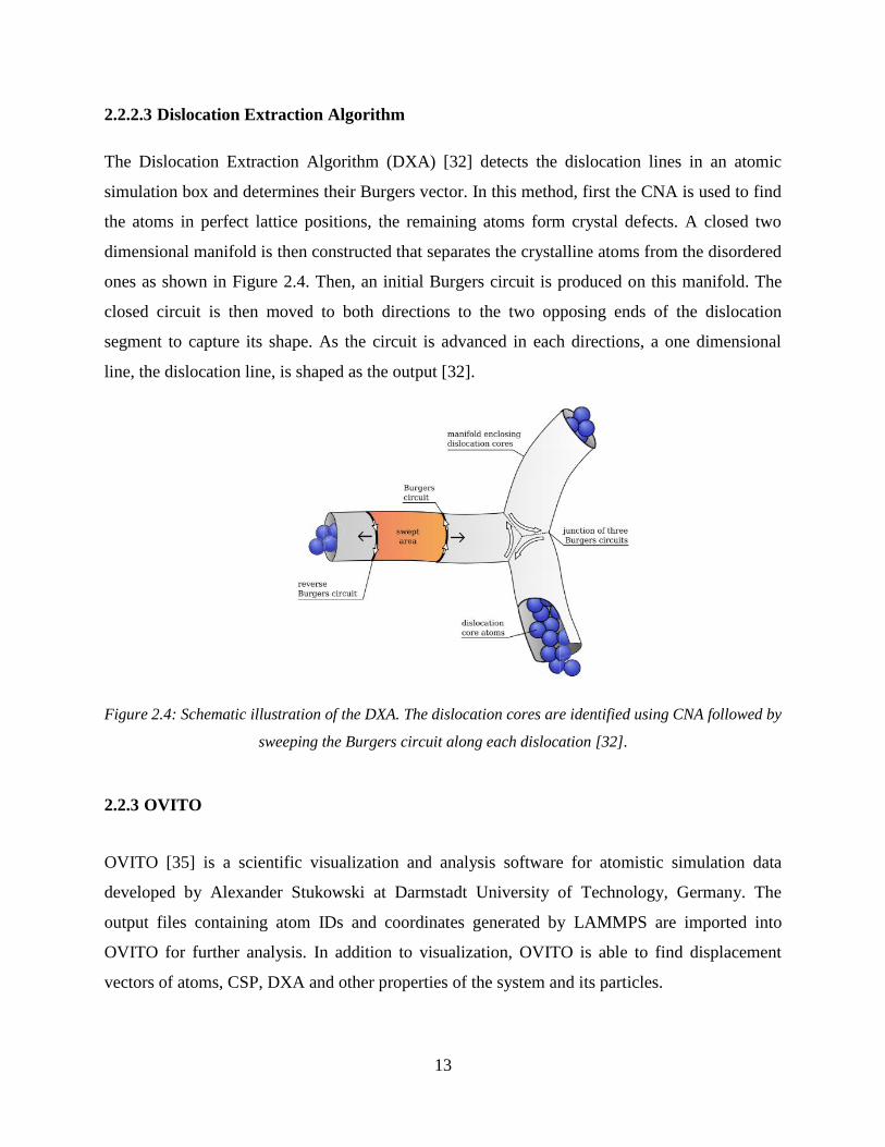
2.2.2.3 Dislocation Extraction Algorithm

The Dislocation Extraction Algorithm (DXA) [32] detects the dislocation lines in an atomic

simulation box and determines their Burgers vector. In this method, first the CNA is used to find

the atoms in perfect lattice positions, the remaining atoms form crystal defects. A closed two

dimensional manifold is then constructed that separates the crystalline atoms from the disordered

ones as shown in Figure 2.4. Then, an initial Burgers circuit is produced on this manifold. The

closed circuit is then moved to both directions to the two opposing ends of the dislocation

segment to capture its shape. As the circuit is advanced in each directions, a one dimensional

line, the dislocation line, is shaped as the output [32].

Figure 2.4: Schematic illustration of the DXA. The dislocation cores are identified using CNA followed by

sweeping the Burgers circuit along each dislocation [32].

2.2.3 OVITO

OVITO [35] is a scientific visualization and analysis software for atomistic simulation data

developed by Alexander Stukowski at Darmstadt University of Technology, Germany. The

output files containing atom IDs and coordinates generated by LAMMPS are imported into

OVITO for further analysis. In addition to visualization, OVITO is able to find displacement

vectors of atoms, CSP, DXA and other properties of the system and its particles.

14

2.3 Diffusion in solids

One of the most fundamental processes that controls the rate at which many transformations

occur is the diffusion in solid state. Atoms can diffuse through a solid by two common

mechanisms, which depends on the site occupied in the lattice: vacancy mechanism, which

happens when substitutional atoms diffuse, and interstitial mechanism which happens when

small interstitial atoms migrate between larger atoms [36].

If an adjacent site to an atom is vacant, a particularly violent oscillation, which depends on

the temperature, results in the atom jumping over onto the vacancy. Therefore, the probability

that any atom will be able to make a diffusive jump depends on the probability that it can acquire

sufficient vibrational energy. Moreover, the rate of migration of an atom through a solid also

depends on the frequency with which it encounters a vacancy, which therefore depends on the

concentration of vacancies. Also, through interstitial mechanism, a small solute atom can migrate

along interstitial site between solvent atoms [36].

The molar diffusion flux of a substance, A, is proportional to the molar concentration

gradient, 𝜕𝐶𝐴

∂x, and diffusion coefficient is the proportionality constant as the first Fick’s law

states [36]:

𝐽𝐴 = −𝐷𝐴𝜕𝐶𝐴

𝜕𝑥 Equation 2.18

where J is the molar diffusion flux and D is the diffusion coefficient. It can be shown that

diffusion coefficient is temperature dependent and follows the Arrhenius law:

𝐷𝐴 = 𝐷0𝐴 exp( −𝐸𝐴

𝑅𝑇 ) Equation 2.19

where 𝐷0 is pre-exponential constant of diffusion coefficient and 𝐸𝐴 is the activation energy of

diffusion. By introducing a radioactive atom into a pure solid, the rate of self-diffusion can be

obtained experimentally [36].

By viewing diffusion as random thermal motion of particles in the system, it is possible to

formulate the diffusion coefficient. More precisely, we can consider the diffusion phenomena, as

15

random walk in which particles move by a sequence of steps with a constant frequency and equal

probability in any direction [37].

The simplest case is a one dimensional system in which particles take steps with length ±𝑙

with equal probability in 𝑧 direction. Assuming jump frequency is constant and directions of

successive jumps are uncorrelated, the probability of a positive step is equal to 1 2⁄ . Therefore,

the mean squared distance of each particle is as follows [37]:

⟨𝑧2(𝑛)⟩ = ⟨(∑ 𝑙𝑖𝑛𝑖=1 )2⟩ = ∑ (𝑙𝑖

2) + ∑ ⟨𝑙𝑖𝑙𝑗⟩𝑖≠𝑗𝑛𝑖=1 Equation 2.20

where 𝑙𝑖 (= ±𝑙) is the resulted displacement of a jump. Since the steps are uncorrelated:

⟨𝑙𝑖𝑙𝑗⟩ = ⟨𝑙𝑖⟩⟨𝑙𝑗⟩ Equation 2.21

and considering ⟨𝑙𝑖⟩ = 0, therefore:

⟨𝑧2(𝑛)⟩ = 𝑛𝑙2 Equation 2.22

on the other hand, 𝑛 =𝑡

𝜏 , where n is the number of steps and t and 𝜏 are time and time between

jumps. Therefore:

⟨𝑧2(𝑛)⟩ = 2𝐷𝑡 Equation 2.23

where ⟨𝑧2(𝑛)⟩ is the mean squared displacement of the particle and 𝐷 is the diffusion

coefficient:

𝐷 =𝑙2

2𝜏

Equation 2.24

This relation is widely used to compute diffusion coefficient from molecular dynamics

simulations [37].

16

2.4 Dislocation diffusion

It has been established that mobility of atoms in the core of atomic dislocations can be much

higher than in perfect lattice sites. The existence of high diffusivity in core regions, also referred

to as “pipe-diffusion”, has been confirmed for metallic, ionic and covalent crystals such as Ag,

Ni, Al, Cu, MgO, UO2 and Si [6].

Pipe diffusion can be the dominant mechanism of mass transport in sintering process. For

example generation of high density of dislocations during the 𝛼 → 𝛽 phase transformation in Ti

enables sintering mass transport through pipe diffusion [38]. Pipe diffusion also enhances the

diffusion of alloying elements. In the proximity of the dislocation core in Cu matrix alloys, the

activation energy of pipe diffusion of alloying elements is estimated to be 70% of the bulk

diffusion value [39]. Dislocation diffusion can also play a significant role in creep mechanisms.

Creep behavior of Fe-C alloys at high temperatures and strain rates is affected by pipe diffusion

of iron in austenite [3]. Also the creep behavior of Sn-3.5Ag solder/Cu couple was found to be

correlated with self-diffusion of pure Sn at high temperatures and dislocation core diffusion at

lower temperatures [40]. Pipe diffusion also causes the formation of solute chains along

dislocations and the dislocations act as solute-pumping stations causing solute atoms to form

linear chains along cores [4].

2.4.1 Formalism

In order to describe diffusion along the dislocation core, the dislocations are represented as pipes

with high diffusivity embedded in a matrix with lower diffusivity. Therefore diffusivity depends

on the structure of the dislocation core which in turn should depend on the Burgers vector of the

dislocation, the direction of the dislocation line and the magnitude of stacking fault energy [2].

Since in FCC metals, dislocation may dissociate into partials, stacking fault energy also should

be considered as an important factor on diffusivity. It is possible to obtain the combined value of

these parameters using [2]:

𝑃𝑑 = 𝐴𝑑𝐷𝑑 Equation 2.25

17

where 𝐷𝑑 is the diffusivity along dislocation core and 𝐴𝑑 is the effective cross sectional area. By

analogy to bulk diffusion equation, it is reasonable to use the following equation for dislocation

diffusion [2]:

𝐷𝑑 = 𝐷𝑑0 exp(

−𝐸𝑑

𝑘𝐵𝑇 ) Equation 2.26

where 𝐸𝑑 is the activation energy for diffusion along the dislocation, and 𝐷𝑑0 is the temperature

independent pre-exponential factor. The effective diffusion coefficient is then [41]:

𝐷eff = 𝐷𝑣𝑓𝑣 + 𝐷𝑑𝑓𝑑 Equation 2.27

where 𝐷eff is the effective diffusion, 𝐷𝑣 is the diffusion coefficient of the lattice, 𝐷𝑑 is the

diffusion coefficient of the core, 𝑓𝑣 is the contribution from the lattice, and 𝑓𝑑 is the contribution

from the core. This equation was modified by Frost and Ashby [42] to get:

𝐷eff = 𝐷𝑣(1 +𝜌𝐴𝑑𝐷𝑑

𝐷𝑣) Equation 2.28

where 𝜌 is the dislocation density.

2.4.2 Experimental measurements

Fast diffusion along dislocation core has been experimentally reported for number of FCC metals

including Al, Cu, Ni, and Ag [2]. Two approaches have been used in experimental studies in

order to measure the diffusivity inside the dislocation core: direct and indirect. In direct

measurements, the diffusion coefficient is extracted from the penetration profile of radioactive

tracer along low angle grain boundaries. In this method, dislocations are represented as pipes

with high diffusivity (normal to the surface and arranged in a wall) with radius rd and diffusion

coefficient 𝐷𝑑. By fitting a model solution to experimental profile, the integrated flux, 𝑃𝑑 =

𝐷𝑑𝐴𝑑 can be obtained [9]. It is usually assumed that diffusivity is only fast in inelastic region of

dislocation core, often a cylinder with 𝑟𝑑 = 0.5 nm, therefore 𝐷𝑑 can be extracted. In indirect

methods, 𝑃𝑑 is back calculated from the rate of a specific process (such as phase growth kinetics

[43] or annihilation of dislocation dipoles [44]) which is assumed to be controlled by pipe-

diffusion. As an example, Volin et al. [45] carried out a quantitative measurement of net mass

18

transport along dislocations by self-diffusion in Al. In this study, thin foils of Al were prepared

which contained isolated spherical voids which were connected to the specimen surfaces by

single dislocations. During annealing, the voids connected to the surface by dislocations shrank

faster than isolated voids. Using the rate of the shrinkage and some assumptions, they were able

to approximate 𝐸𝑑 and 𝑃𝑑. A comprehensive summary of experimental results can be found in

[2].

2.4.3 Simulation Studies

Simulation studies on pipe-diffusion are mainly performed by introducing a point defect (a

vacancy or an interstitial) in the core and following the migration path of the defect based on the

assumption that diffusion is only mediated by atomic exchanges with the point defect. Using an

MD study, Huang et al. [13] found the migration energy of diffusion of a vacancy and an

interstitial along a dissociated edge dislocation in copper by introducing these point defects in the

core and counting the jump events at different temperatures. Formation energies of point defects

can also be found using other simulation techniques at 0 K. As a result, activation energy of

diffusion of a point defect along dislocation core, which is the sum of migration energy and

formation energy, can be found.

2.4.4 Mechanisms of pipe-diffusion

Most of the experimental and simulation results confirm that activation energy of pipe-diffusion,

𝐸𝑑 , is about 0.4 to 0.7 of the activation energy of bulk diffusion. Three mechanisms have been

proposed that can contribute to enhancing the diffusion: vacancy mechanism [45], interstitial

mechanism [8] and intrinsic mechanism [9]. Vacancy and interstitial mechanisms have been

related to lower formation or migration energies of these point defects in the core regions [13].

Vegge et al. [46] found that migration of a vacancy near the partial cores of dissociated edge

dislocations in copper occurs easier than in the bulk. The energy barrier was found to be

substantially lower in both compressive and tensile regions of dislocation than in the bulk as

shown in Figure 2.5. The lowest migration barriers were found in the [1̅ 0 1̅] and [0 1 1̅]

19

directions. The vacancies can therefore migrate in the [1̅ 1 2̅] direction by zig-zagging up along

the dislocation line in the [1̅ 0 1̅] and [0 1̅ 1] directions, respectively [46].

Figure 2.5: (a) The atomic configuration; (b) the stress field, where red shows the tensile and blue

indicates the compressive region; right: the barriers for diffusion in the compressive (1) and tensile (2)

regions in the vicinity of partial dislocation cores and in the stacking fault ribbon (3) [46].

By obtaining the activation energy of diffusion of a single vacancy and an interstitial along the

dissociated edge dislocations in copper, Huang et al. [13] asserted that vacancies and interstitials

contribute comparably to pipe-diffusion. The ratio of activation energies for both vacancy and

interstitial mechanisms were found to be 𝐸𝑑 𝐸𝑏⁄ = 0.7 − 0.85. Therefore, it was asserted that the

interstitial mechanism in addition to vacancy mechanism can contribute to enhancing the

diffusion along dislocation core.

The third mechanism of diffusion along the core is known as intrinsic mechanism. In this

mechanism, diffusion occurs along the core, even without any pre-existing point defects in the

structure. Although the existence of intrinsic diffusion has been found by Pun et al. [9], no

comprehensive explanation for this mechanism has been provided. Pun et al. [9] proposed that

the intrinsic diffusion can be associated with the formation of Frenkel pairs (vacancy-interstitial

pair) in core due to thermal fluctuations in the dislocation core. By migrating along the core, the

two defects produce self-diffusion before they recombine. It was found that at high temperatures,

the dislocation becomes a source of point defects and therefore the effect of pre-existing point

defects is small. They also observed that screw dislocation forms dynamic jogs at high

temperatures. Therefore, they hypothesized that “the thermal jogs might be involved in the

Frenkel pair formation” [9].

20

In FCC metals, dislocations on {111} planes tend to dissociate into partial dislocations

with a stacking fault ribbon in between. In the case of perfect dislocations with total 𝑏 =

𝑎 2⁄ ⟨110⟩ diffusion is slowed by dissociation into partial dislocations with the smaller Burgers

vectors 𝑏 = 𝑎 6⁄ ⟨112⟩ [2]. There are reports indicating that diffusivity decreases as dissociation

distance between partials increases. This behavior has been attributed to spread of diffusion into

the whole stacking fault ribbon [8,47] or decreased magnitude of Burgers vector and local

distortion as dislocations relax by dissociation [2]. It should be mentioned that there is not a

definite agreement on the possibility of enhanced diffusion in the stacking fault ribbon. Balluffi

[2] argues that since stacking fault ribbon has HCP structure and nearest neighbor relations

(packing) are conserved in this region, therefore high diffusivity is not possible in the stacking

fault ribbon. On the other hand, other researchers [8] claim that at high temperatures, the disorder

increases and the core becomes larger, therefore there is almost an overlap of the core with the

stacking fault ribbon, hence, diffusion can be fast in this region as well.

2.5 Motivation

The existence of intrinsic diffusion has been only confirmed in Al, an FCC metal with high

stacking fault energy. Since FCC metals with low stacking fault energies have typically larger

dissociation widths, an interesting topic of study is to investigate the possibility of intrinsic

diffusion in metals with low stacking fault energies. The purpose of the present study is to

investigate the possibility of self-intrinsic-diffusion along screw dislocation core in FCC metals,

and analyze the relation between stacking fault energy and diffusivity along the dislocation core.

Identifying the effect of stacking fault energy on the extent of pipe-diffusion is of particular

interest, due to the importance of this phenomenon on dictating kinetics of various processes in

materials. To achieve the above objective, diffusion behavior in dislocation containing single

crystals with different level of stacking fault energies is studied through Molecular Dynamics

(MD) simulations.

21

CHAPTER 3: SIMULATION PROCESS

3.1 Simulation set up

MD simulation is performed using LAMMPS package [28] and embedded atom method (EAM)

potentials. Simulation studies have been conducted on four FCC metals: aluminum, copper,

nickel and silver. These metals are selected because of their high (i.e. Al and Ni), medium (i.e.

Cu) and low (i.e. Ag) stacking fault energies. The EAM potentials used for these elements are

described in [48–51] and accurately predict the values of stacking fault energies and activation

energies of bulk diffusion for the chosen metals. Melting temperatures predicted using these

potentials are 1042 K for Al, 1327 K for Cu, 1715 for Ni and 1267 K for Ag.

In order to study self-diffusion along a screw dislocation core in each of these elements, a

cylindrical model with periodic boundary conditions along z axis is created. 𝑥, 𝑦 and 𝑧 are

parallel to [1̅ 1 2̅], [1̅ 1 1], and [1 1 0] crystallographic directions, respectively. The cylinder has

the length of about 50 Å and diameter of about 150 Å. The approach described in [24] is used to

create a straight screw dislocation along the z direction. In a perfect crystal, positions of atoms

are described by crystal`s Bravais lattice and lattice constant. However, introducing a dislocation

distorts the perfect crystal structure and moves atoms to new positions. To describe this distorted

structure, displacement of atom 𝑖 is 𝑢𝑖 = 𝑥𝑖′ − 𝑥𝑖 where 𝑥𝑖 and 𝑥𝑖

′ are initial and final positions

respectively [24]. Assuming distortion in the crystal is small enough, 𝑢𝑖 can be obtained using

linear elasticity. The position of atoms, 𝑥𝑖, is a continuous variable and 𝑢𝑖 = 𝑥𝑖′ − 𝑥𝑖 is the

displacement field. For our purpose we can use the continuum solution u(x) to approximate the

displacement vector which is 𝑢𝑖 ≈ 𝑢(𝑥𝑖) [24].

Having a screw dislocation along the axis of a cylinder (Figure 3.1), it is evident in that the

only non-zero component of displacement is 𝑢𝑧 and the displacement 𝑢𝑧 is discontinuous at the

cut surface defined by 𝑦 = 0, 𝑥 > 0 [52]:

𝑙𝑖𝑚𝜂→0, 𝑥>0

𝑢𝑧(𝑥, − 𝜂) − 𝑢𝑧(𝑥, 𝜂) = 𝑏𝑧, 𝜂 positive Equation 3.1

22

where 𝑏 is the Burgers vector. It is reasonable to assume that in an isotropic medium, the

displacement 𝑢𝑧 increases uniformly with the angle 𝜃 to yield to this discontinuity [52]:

𝑢𝑧(𝑟, 𝜃) = 𝑏𝜃

2𝜋= 𝑏

𝜃

2𝜋tan−1 𝑦

𝑥 Equation 3.2

where −𝜋 < 𝜃 < 𝜋 is the ange between the horizontal axis and the vector connecting to (𝑥, 𝑦, 0)

[52].

Figure 3.1: a screw dislocation along axis of a cylinder of radius R and Burgers vector b [52]. 𝝃 is the

direction of the dislocation line.

Therefore, in order to create a screw dislocation for each of elements under study, a cylindrical

model with periodic boundary conditions along the 𝑧 axis is created. Axes 𝑥, 𝑦 and 𝑧 are parallel

to [1̅ 1 2]̅, [1̅ 1 1], and [1 1 0] crystallographic directions, respectively. The cylinder has the

length of about 50 Å and diameter of about 150 Å. All atoms are displaced from their initially

perfect lattice positions according to the isotropic linear elasticity solution for a straight screw

dislocation with the Burgers vector 1 2⁄ [1 1 0].

A smaller cylinder is cut out from this cylinder, with the same length and a smaller

diameter of about 70 Å, with about 10,000 atoms. The structure containing a screw dislocation

with Burgers vector 1 2⁄ [1 1 0] is shown in Figure 3.2.

23

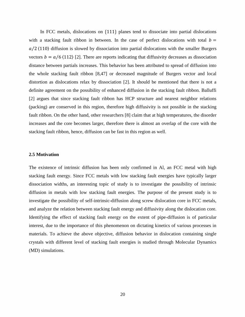
Figure 3.2: A slice parallel to dislocation line shown

with red segment. Green atoms represent atoms in perfect FCC structure.

Atoms within a 10 Å thick outer layer of this cylinder are fixed and all other atoms are relaxed at

0 K using conjugate gradient method implemented in LAMMPS to bring the system to

equilibrium state. This method relaxes the system by minimizing the total potential energy with

respect to atomic positions. An example of such relaxation is shown in Figure 3.3 in Al, where

the potential energy of the system decreases during relaxation and the system is brought to

equilibrium state at 0 K.

24

(c)

Figure 3.3: Relaxation of a system containing a screw dislocation in Al.

(a) Initial structure with the dislocation core at the center of the cylinder.

Atoms in core regions have higher potential energy

(b) the relaxed structure (c) the potential energy of the system decreases

during relaxation to bring the system to equilibrium state

Upon relaxation, in all elements under study, the dislocation dissociates into two Shockley

partials on {111} plane, as expected. The dissociation can be visualized using DXA feature

implemented in OVITO. In Al, the dissociation width is very narrow (because of its high

stacking fault energy) and the distance between partial dislocations is only about 7 Å (about

25

2.5𝑏), whereas the dissociation widths for Ni, Cu and Ag are about 9 Å (about 3.5𝑏), 13 Å

(about 5𝑏) and 25 Å (about 8.5𝑏), respectively as shown in Figure 3.4. These values follow the

general fact that the degree of dissociation increases with decreasing stacking fault energy and

are in agreement with earlier experimental and simulation results [53,54]. In order to efficiently

perform MD runs with small number of atoms, more atoms on the outer layer of the cylinder are

fixed. Free atoms are located in a cylinder with diameter of about 30 Å to 50 Å, depending on the

element under study.

Figure 3.4: Relaxed structures of the dislocation in (a) Al, (b) Ni, (c) Cu and (d) Ag. A slice of the

simulation box parallel to the dislocation line is shown. Green and red atoms represent FCC and HCP

structures (stacking fault) respectively. Blue segments show partial dislocations.

Diffusion has been studied at constant temperatures between 800 K to 1000 K for Al, 1500 K to

1600 K for Ni and 1250 K to 1325 K for Cu. A series of MD runs close to melting point, 1267

K, are also performed for Ag. With respect to the chosen temperature, the simulation box is

expanded uniformly before MD runs in order to minimize the thermal stresses at high

temperatures. Using NVT (constant number of particles, volume and temperature) ensemble and

a time step of 2 femtoseconds, the temperature is increased to a desired value during first 1

nanosecond followed by an isothermal annealing for 30 ns to 60 ns, depending on the

temperature and the element under study. It should be emphasized that no vacancy (or

interstitial) is introduced into the system; therefore any diffusion observed at high temperatures

is related to the intrinsic diffusion.

26

CHAPTER 4: RESULTS AND DISSCUSSION

4.1 Activation energy of pipe diffusion

To test the validity of simulations, total energy (𝐸 = potential energy + kinetic energy) of the

system, in NVE ensemble is checked. This value must be conserved in NVE (constant number of

atoms, volume and energy) ensemble, however small fluctuations are allowed because of the

errors in integration of Newton’s equations of motion. As an example of such calculations, in

Figure 4.1, the structure of Al is brought to 1000 K during the first 1ns using NVT ensemble

followed by 1ns of NVE ensemble at 1000 K. This confirms fluctuations in total energy are

negligible.

Figure 4.1: Total energy vs. time in Al during 1ns of NVE ensemble at 1000 K.

High mobility of atoms along the dislocation core was observed at high temperatures in Al, Ni

and Cu, even without any pre-existing point defects in the structure. Figure 4.2 shows a slice of

the simulation box where atoms are color coded using absolute displacement magnitude along 𝑧

axis after 30 ns of isothermal annealing in each of the elements under study. Although high

mobility is found along z axis, [110], the displacements of atoms along 𝑥 and 𝑦 directions are

-32409.8

-32409.72

-32409.64

-32409.56

-32409.48

-32409.4

-32409.32

0.8 1 1.2 1.4 1.6 1.8 2 2.2

tota

l en

erg

y (e

V)

time (ns)

27

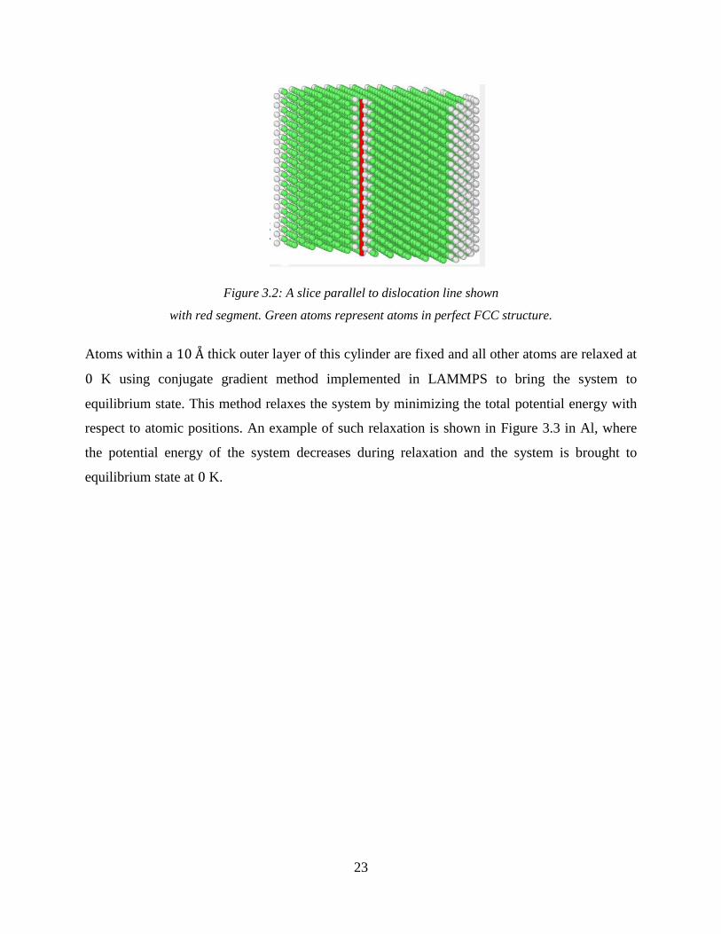
very small during annealing. In Ag, no enhanced diffusion was detected even along the

dislocation line, 𝑧 axis.

Figure 4.2: A slice of cylinder parallel to the dislocation line (a) Al at 900 K (0.86Tm), Ni at 1550 K (0.9

Tm), (c) Cu at 1300 K (0.98 Tm) and (d) Ag at 1150 K (0.9 Tm). Atoms are color coded using the absolute

displacements along the dislocation line (z axis) after 30 ns of isothermal annealing. Figures are

obtained by OVITO. The dislocation core is at the center of the cylinder.

In each of the elements understudy, the results of MD simulations are analyzed following the

method proposed in [9] to find the pre-exponential factor, 𝐷𝑑0, and activation energy of self-

diffusion along the core, 𝐸𝑑 in Equation 2.26. First it is needed to find the diffusion coefficient at

a given temperature as a function of distance from the dislocation core. To do so, imaginary

cylinders with radii 𝑅, ranging from 5 Å to 13 Å centered at midpoint between partials are

chosen, as shown in Figure 4.3.

28

Figure 4.3: Top view of the simulation cell. Imaginary cylinders with different radii ranging from 5Å to

13Å, centered at midpoint between partials are chosen.

The diffusion coefficient in each of the cylinders can be found using the Einstein formula for

diffusivity:

𝑀𝑆𝐷 = ⟨[𝑧(𝑡0) − 𝑧(𝑡0 + 𝑡)]2⟩ = 2𝐷𝑡 Equation 4.1

where 𝐷 is the diffusion coefficient, t0 is time origin, 𝑡 is time and ⟨ ⟩ averages over all atoms in

the chosen cylinder and all time origins (any time step can be considered time zero, 𝑡0, in

Equation 4.1). 𝑀𝑆𝐷 is the Mean Squared Displacements of atoms along the dislocation line for

atoms located in each cylinder. Therefore, 𝐷 in each of the cylinders, can be found using the

slope of MSD vs. time. Next, by plotting 𝐷 vs. the radius, 𝑅, at different temperatues, it is

possible to find the activation energy of self-diffusion along the dislocation core in each of the

elements, as proposed in [9].

In order to plot 𝑀𝑆𝐷 vs. time for atoms in a cylinder, isothermal annealing time (30 ns) is

divided into 10 shorter time intervals (3 ns). For each interval, the value of 𝑀𝑆𝐷 at each time

step is calculated and plotted vs time. These values are then averaged over the 10 time intervals

(Figure 4.4) to get better statistics. Note that an atom attempting to leave the simulation box

immediately re-enters from the opposite face because of the periodicity in 𝑧 direction (e.g.

wrapping procedure), however, in calculating 𝑀𝑆𝐷s, unwrapped coordinates of atoms must be

used to get true displacements of atoms.

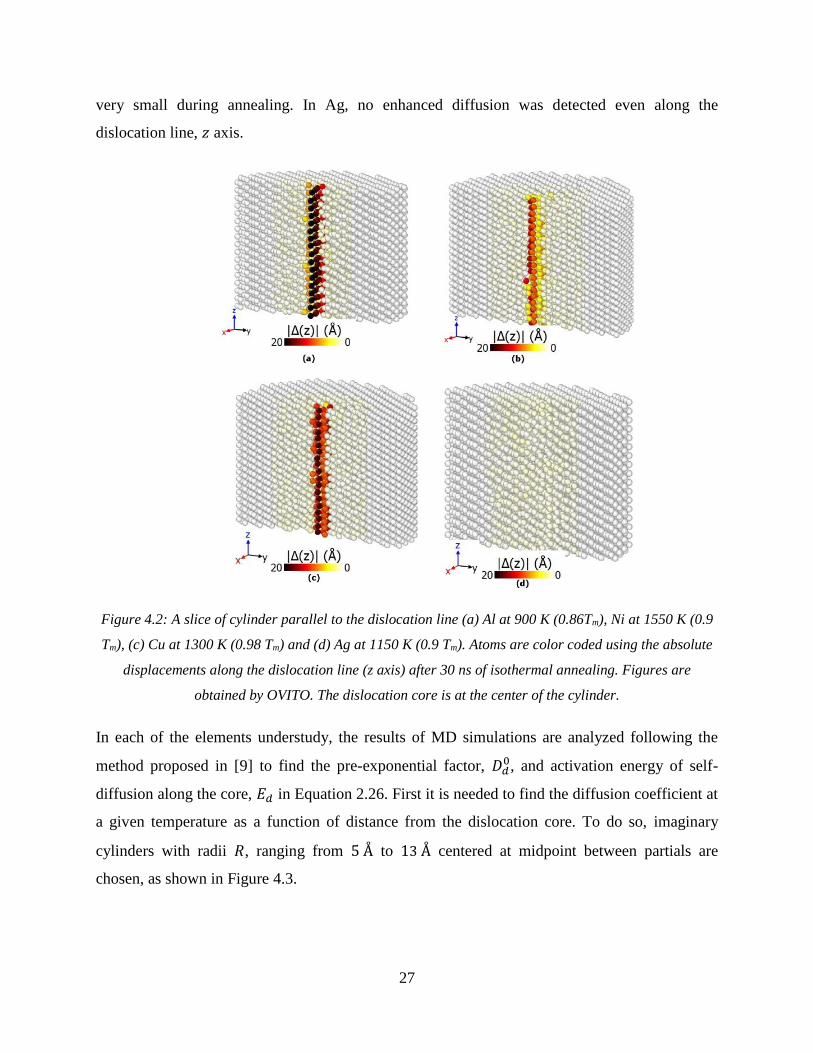
29

Figure 4.4: Mean squared displacements along the core of a screw dislocation in (a) Al at T=900 K, (b)

Cu at T=1300 K and (c) at T=1550K for Ni. The displacements are shown for different values of radius,

R.

30

In the case of Ag, the 𝑀𝑆𝐷 of atoms is very small and not representative of diffusion, but only

thermal fluctuations, even at high temperatures close to the melting point and long MD runs.

This shows that the intrinsic diffusivity is not remarkable in Ag, therefore, the results are not

reported for Ag. The plots in Figure 4.4 show a linear trend for 𝑀𝑆𝐷 as a function of time. The

diffusion coefficient in a cylinder can be calculated using Equation 4.1. Values obtained for 𝐷 at

each temperature are then plotted vs. the chosen radius, 𝑅, as shown in Figure 4.5.

Figure 4.5: Average diffusivity vs. R for (a) Al (b) Cu and (c) Ni.

31

It can be observed in Figure 4.5 that the diffusivity averaged over a cylindrical region decreases

as the distance from the dislocation core, 𝑅, increases. These plots are best described by

Gaussian function [9]:

𝐷 = 𝐴𝑒

−𝑅2

𝑟𝑑2

+ 𝐵 Equation 4.2

with adjustable parameters 𝐴, 𝐵 and 𝑟𝑑. 𝐵 is negligible, but not zero due to the effect of

boundary conditions and 𝑟𝑑 is considered as the dislocation core radius [9]. Therefore with 𝑅 =

𝑟𝑑, dislocation diffusivity, 𝐷𝑑, at each temperature is approximately equal to [9]:

𝐷𝑑 ≈ 𝐴 𝑒⁄ Equation 4.3

Dislocation diffusivities for temperatures simulated are calculated and reported in Appendix one.

Dislocation diffusivities are then fitted to the Arrhenius equation as shown in Figure 4.6, and

activation energies for diffusion inside the dislocation core are calculated for Al and Cu and Ni,

as reported in Table 4.1.

32

Figure 4.6: Diffusion coefficients inside the screw dislocation core at each temperature and fitted to

Arrhenius law for (a) Al and (b) Cu and (c) Ni.

Table 4.1: Calculated separation distance of dislocations (𝑑), pipe-diffusion activation energy (𝐸𝑑),

integrated diffusion flux (𝑃𝑑0) and pre-exponential factor of pipe-diffusion (𝐷𝑑

0). Stacking fault energies

(𝐸𝑠𝑡𝑘_𝑓𝑙𝑡) and bulk diffusion activation energies (𝐸𝑏) are obtained from EAM potentials [48–51].

Element Estk_flt

(𝑚𝐽 𝑚−2)

𝑑

(Å)

𝐸𝑏

(𝑒𝑉)

𝐸𝑑

(𝑒𝑉)

𝑃𝑑0

(𝑐𝑚4𝑠−1)

𝐷𝑑0

(𝑐𝑚2𝑠−1)

𝐸𝑑/𝐸𝑏

Al 146 [49] 7 1.2 [49] 0.57 2.3x10-18 2.1x10-4 0.48

Ni 134 [21] 9 2.76 [21] 1.58 5.9 x 10-17 5.3x10-3 0.57

Cu 45 [19] 13 1.96 [50] 1.61 4.6 x10-16 4.1 x10-2 0.82

Ag 17 [20] 25 1.76 [51] - - - -

33

The results show existence of intrinsic diffusivity along the screw dislocation core in Al, Ni

and Cu. The activation energy of self-intrinsic-diffusion, i.e. diffusion along screw dislocation

through intrinsic mechanism, for copper is found to be about 1.61 𝑒𝑉, which is slightly smaller

than the activation energy of self-diffusion in bulk (𝐸𝑏 = 1.96 𝑒𝑉). The smaller activation

energy suggests that inside the core regions of dislocation in copper, diffusion can be enhanced

through intrinsic mechanism. For aluminum, 𝐸𝑑 was found to be about 0.57 𝑒𝑉, which is

significantly lower than the activation energy of self-diffusion in bulk (𝐸𝑏 = 1.2 𝑒𝑉), meaning

that intrinsic mechanism along dislocations core can be a major diffusion process for Al. This is

also the case for Ni, where, 𝐸𝑑 was found to be about 1.58 𝑒𝑉 much lower than 𝐸𝑏 = 2.76 𝑒𝑉.

Radius of high diffusivity pipe, 𝑟𝑑 in Equation 4.2, for all three cases, Al, Ni and Cu is

found to be about 6 Å (in all materials understudy and independent of temperature), which is in

good agreement with 𝑟𝑑 = 5 Å proposed through experimental studies [2]. The results for Al are

also in good agreement with the simulations done earlier [9] on self-diffusion along screw

dislocation core. However for Cu, Ni and Ag, there are no previous simulations on screw

dislocation pipe diffusion to compare. The only experimental data available on self-pipe-

diffusion of Cu is the estimation done by Balluffi [2]. Based on the experimental results of Oren

and Bauer [55] on diffusion of germanium solute atoms along dissociated dislocations in copper,

Balluffi [2] calculated the pip-diffusion to bulk diffusion activation energy ratio (i.e. 𝐸𝑑/𝐸𝑏) and

𝑃𝑑0, to be about 0.8 and 1.04 × 10−16 cm4 s−1, respectively [2]. For diffusion along dissociated

edge dislocations in copper, Huang et.al [8] found 𝐸𝑑/𝐸𝑏 = 0.8 and 𝑃𝑑0 = 1.8 × 10−15 cm2 s−1

for vacancy mechanism, and 𝐸𝑑 𝐸𝑏⁄ = 0.7 and 𝑃𝑑0 = 2.9 × 10−16 cm2 s−1 for interstitial

mechanism. The values obtained in the present work (reported in Table 4.1) are also close to

these results. Considering the ratio of 𝐸𝑑 𝐸𝑏⁄ being less than unity for Al, Ni, and Cu, in addition

to the fact that no enhancement of diffusion has been detected for Ag, it is suggested that with

increasing the stacking fault energy in FCC metals, the effect of screw dislocation on enhancing

the diffusion becomes more remarkable.

Interestingly, we observed that in intrinsic mechanism, diffusion occurs by migration of the

entire rows of atoms (located in a pipe with radius of about 6 Å), along the dislocation line, as

demonstrated in Figure 4.7. No evidence of spread of diffusion in the stacking fault ribbon is

34

observed. Instead, the region of high diffusivity is found to be within a pipe with radius of about

6 Å centered at midpoint between partial dislocations.

Figure 4.7: diffusion of atoms along the dislocation line in Al at 900 K after 30 ns in a cylinder

with 𝑅 = 11 Å. The unwrapped coordinates of atoms are shown.

By visualization of partial dislocations configurations in random snapshots of MD runs, we

observed that partial dislocations are able to frequently reverse and form a full dislocation

(constriction) in Al and Ni as shown in Figure 4.8(a) and Figure 4.8(b). However, in Ag,

Figure 4.8(d), the separation distance between partial dislocations is so high that the chance of

the constriction of the partials into a full dislocation is very small. We could not detect any

constriction of the partials in Ag, even at high temperatures. In Cu, Figure 4.8(c), although the

distance between partials is relatively high at most of the snapshots, constriction of partial

dislocations have been detected at some of the snapshots. It should also be noted that when

partial dislocations constrict into a full dislocation, the magnitude of Burgers vector and hence

the distortion increases locally.

35

(a) (b)

(c) (d)

Figure 4.8: A slice of cylinder parallel to z axis and configuration of partial dislocations at a random

snapshot for (a) Al at 900 K (0.86Tm) (b) Ni at 1550 K (0.90 Tm), (c) Cu at 1300 K (0.98 Tm) and (d) Ag at

1150 K (0.9 Tm).

In addition, recurrent formation and migration of point defects were observed along the core.

Formation of point defects can be detected using Wigner-Seitz defect analysis employed in

OVITO [35]. In this method, each atom in the reference configuration (here, the relaxed structure

with partial dislocations at 0 K), defines the center of a Wigner-Seitz cell, which is the spatial

region belonging to that site. Any atom from the displaced configuration (which is any snapshot

of the structure during the annealing) that is located within the Wigner-Seitz cell of a reference

site is said to occupy that site. The modifier then outputs the number of atoms occupying a site.

36

As shown in Figure 4.9, typically all sites are occupied by one atom (color coded with green).

However, it can be observed that at some snapshots, there are sites occupied by zero atoms (e.g.

vacancy formation, color coded with blue in Figure 4.9,). Some sites are also occupied by two

atoms (e.g. interstitial formation, color coded with red). This observation suggests that at high

temperatures, the dislocation core becomes an effective source for point defect generation. As

shown in Figure 4.9(a), first a pair of vacancy-interstitial forms. These two defects separate and

start to migrate along the core as shown in Figure 4.9(b), giving rise to diffusivity, and finally

recombine and restore the defect-free structure (see Figure 4.9(c)). Figure 4.9(d) shows high

number of point defects formation in the core at high temperatures.

Figure 4.9 Wigner-Seitz defect analysis: (a) formation of a vacancy-interstitial (b) these two point defect

briefly separate and migrate along the core (c) vacancy and interstitial recombine (d) formation of

vacancy-interstitial pair in core regions at high temperatures

The observations illustrated in Figure 4.8 and Figure 4.9 may suggest that the diffusion in the

absence of any pre-existing point defects occur when partial dislocations with Burgers vector

1 6⁄ ⟨112⟩ are able to recombine and form a full dislocation of 1 2⁄ ⟨110⟩ kind where point

defects form and start to migrate along the core.

37

4.2 Vacancy formation energy

In order to evaluate this hypothesis, it is helpful to find the vacancy formation energy along the

partial dislocations and compare these values to vacancy formation energies in the bulk. To find

vacancy formation energy, 𝐸𝑣𝑓, a single vacancy is created inside the system (that contains a

relaxed screw dislocation) at different sites in the structure by deleting the particular atom

occupying the site. The simulation box is then relaxed statically at 0 K. From the energy

difference between the relaxed system with a vacancy and the initial relaxed system without a

vacancy, 𝐸𝑣𝑓

is found using:

𝐸𝑣𝑓

= 𝐸𝑓 − [𝑁−1

𝑁] × 𝐸𝑖 Equation 4.4

where 𝐸𝑓 is the energy of the relaxed system containing a vacancy, 𝐸𝑖 is the energy of the

relaxed system without a vacancy and N is the number of atoms in the initial system. Figure 4.10

shows the values of vacancy formation energy at different sites in the simulation box for copper.

The minimum value found was 1.09 𝑒𝑉, which was found on atomic sites close to the partial

dislocations. This value is about 0.86 of vacancy formation energy in the bulk copper, 𝐸𝑏 =

1.27 𝑒𝑉.

Figure 4.10: Vacancy formation energy in the vicinity of the partial dislocations (green colored circles)

in copper.

38

These results suggest that the distortion introduced at each site by the partial dislocations

decreases the formation energy of vacancy. However, formation energy of vacancy should also

be calculated on full dislocations as well, in order to compare the value with the value obtained

on partial dislocations (which can be an interesting subject for future work).

4.3 Contribution of vacancy mechanism to diffusion along a screw dislocation core

In order to compare the contribution of the intrinsic mechanism and the contribution of the

vacancy mechanism to diffusion along the core, a single vacancy is created inside the system

(that contains a relaxed screw dislocation) at a random site of copper structure. It should be

emphasized that by vacancy mechanism, we are referring to the diffusion along the core in the

presence of equilibrium number of vacancies, whereas the intrinsic mechanism is referred to the

diffusion along the core without any pre-existing point defects.

The same approach discussed in section 4.1 is used to calculate the diffusion coefficient at

each temperature as a function of R, the radius of imaginary cylinders in copper, as shown in

Figure 4.11. However, since the system contains one vacancy, the raw values of diffusion

coefficient, 𝐷𝑑raw, need to be corrected for the equilibrium number of vacancies at each

temperature using Equation 4.5.

Figure 4.11: Average diffusivity vs. R with a single vacancy and a screw dislocation in the system in Cu.

39

At all temperatures studied here, the simulation box contains one vacancy, which stays in the

core regions most of the time. It also spends a fraction of time in surrounding lattice regions but

diffuses relatively slowly. It should be noted that the fixed boundaries prevent the vacancy to

leave the simulation box in the x and y directions.

The calculations of the diffusion coefficient in the presence of equilibrium number of

vacancies, requires the knowledge of average number, 𝑁𝑣, of vacancies that would be found in

the simulation box at equilibrium at a given temperature. 𝑁𝑣 can be found using [9]:

𝑁𝑣 = ∑ exp (−𝐸𝑣

𝑓

𝑘𝐵𝑇) 𝑁

𝑛=1 . Equation 4.5

where 𝐸𝑣𝑓

is the vacancy formation energy at site n and can be found using Equation 4.4 and the

summation runs over all N positions of the dynamic atoms. Using 𝑁𝑣, calculated using

Equation 4.5, it is possible to correct the value of raw diffusion coefficient, 𝐷𝑑raw, to find true

dislocation diffusivity by [9]:

𝐷𝑑𝑣 = 𝐷𝑑

𝐼 + 𝑁𝑣(𝐷𝑑raw − 𝐷𝑑

𝐼 ). Equation 4.6

where 𝐷𝑑𝑣 is the corrected value of dislocation diffusivity in the presence of equilibrium number

of vacancies, 𝐷𝑑𝐼 is the contribution of the intrinsic diffusion to diffusivity assuming the intrinsic

diffusion continues to operate in core regions. 𝐷𝑑𝐼 is calculated earlier as shown in Figure 4.6.

The second term in the equation above is the contribution of vacancy mechanism.

Figure 4.12 shows the values of true dislocation diffusivity along the dislocation core in

copper after corrections for equilibrium number of vacancies. It can be observed that the

contribution of vacancy mechanism is small compared to intrinsic diffusion, since the values of

𝐷𝑑𝑣 are only slightly larger than 𝐷𝑑

𝐼 . A similar result was obtained by Pun et al. [9] for

contribution of vacancy mechanism to diffusion along the dislocation core in Al. This result

again suggests that the dislocation core becomes an effective source of point defect generation to

a degree that the contribution of pre-existing point defects becomes negligible, at the

temperatures studied here.

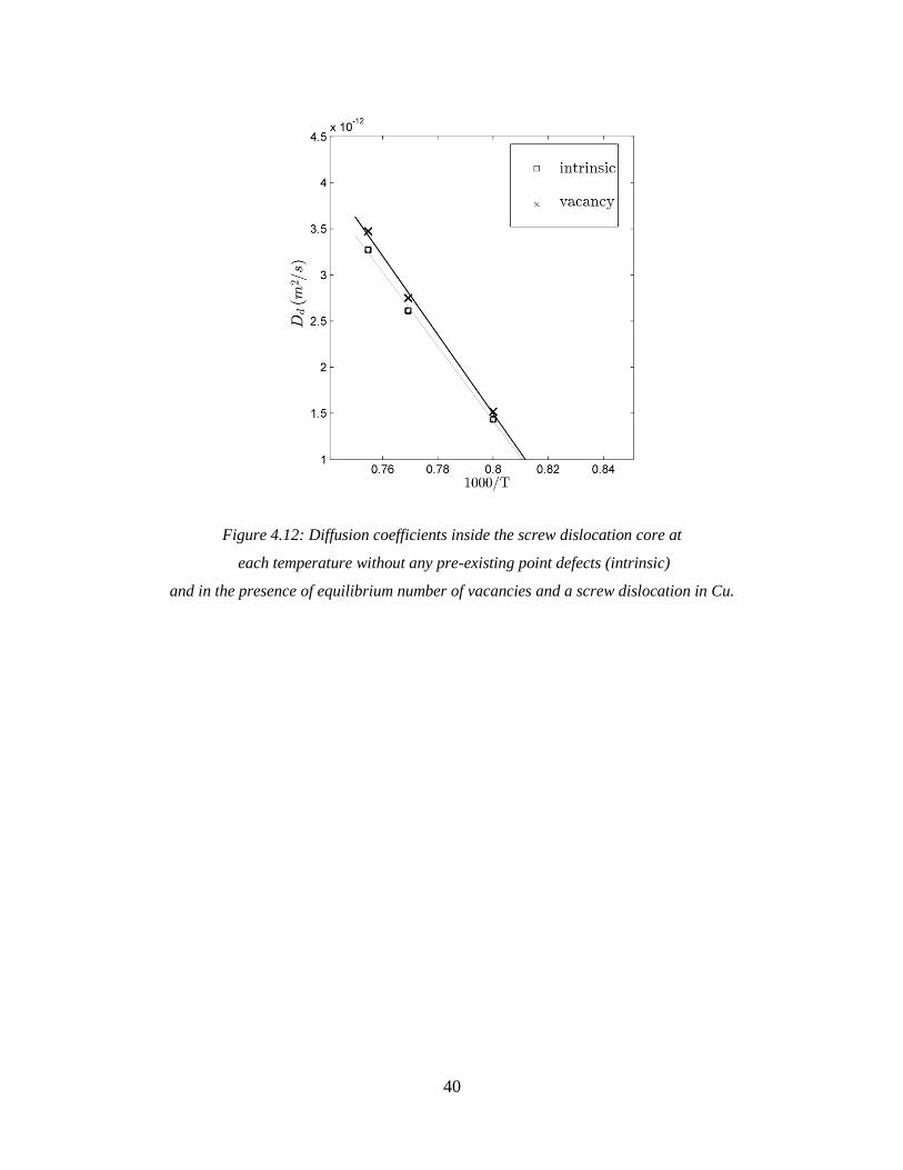
40

Figure 4.12: Diffusion coefficients inside the screw dislocation core at

each temperature without any pre-existing point defects (intrinsic)

and in the presence of equilibrium number of vacancies and a screw dislocation in Cu.

41

4.4 Conclusion

In summary, our results confirms observation of high diffusivity along the screw dislocation core

in Al, Ni and Cu even without any pre-existing point defects,. Since the enhancement in

diffusivity is more remarkable in Al and Ni (high stacking fault energy) than in Cu, and the fact

that no high diffusivity was observed along the core in Ag, it is suggested that the diffusivity

strongly depends on the magnitude of stacking fault energy and the dissociation distance

between partial dislocations.

It was observed that during isothermal annealing, the partial dislocations frequently reverse

and form a full dislocation in Al and Ni. The frequency of recombination of partials is lower in

Cu. Moreover, recurrent formation and migration of point defects along the core were detected

during the isothermal annealing. It is suggested that the formation of point defects might be

related to the reversion of partial dislocations into a full dislocation where a vacancy forms and

starts to migrate along the core. By calculating the vacancy formation energy in the vicinity of

partial dislocations, it was found that the vacancy formation energy is lower along partial

dislocations than in bulk.

The contribution of vacancy mechanism to diffusion along the core was also measured by

introducing a vacancy in the system and accounting for the equilibrium number of vacancies at

each temperature. We found that diffusion coefficient is only slightly larger in the presence of

vacancy, hence the contribution of vacancy mechanism is negligible compared to the intrinsic

mechanism. This fact suggests that the screw dislocation core becomes an effective source of

point defect generation to the extent that the effect of pre-existing point defects becomes

negligible.

4.5 Future work

An interesting topic of the future research would be to find the formation energy of point defects

on full dislocations and compare the value to the value in bulk and the value obtained on partial

dislocations. If lower formation energy of point defects is obtained on full dislocations than on

partial dislocations, it might confirm that reversion of partial dislocations into a full dislocation

42

at high temperatures, results in generation and migration of the defects along the core, which

gives rise to diffusion. Another interesting approach would be to find the activation energy of

diffusion along full dislocations rather than dissociated dislocations.

43

References

[1] H. Mehrer, Diffusion in Solids: Fundamentals, Methods, Materials, Diffusion-Controlled

Processes, Springer Science & Business Media, Berlin, 2007.

[2] R.W. Balluffi, Phys. Status Solidi 42 (1970) 11–34.

[3] D. Lesuer, C. Syn, J. Whittenberger, M. Carsí, Mater. Sci. 317 (2001) 101–107.

[4] R. Schwarz, Mater. Sci. Forum 269 (1998).

[5] M. Kolbe, A. Dlouhy, G. Eggeler, Mater. Sci. Eng. A 246 (1998) 133–142.

[6] R.W. Balluffi, A.V. Granato, in:, Dislocations Solids Ed. FRN Nabarro, North-Holland,

New York, 1979.

[7] Z. Wang, G. Shiflet, Metall. Mater. Trans. A 29 (1998) 2073–2085.

[8] J. Huang, M. Meyer, V. Pontikis, Philos. Mag. A 63 (1991) 1149–1165.

[9] G.P. Purja Pun, Y. Mishin, Acta Mater. 57 (2009) 5531–5542.

[10] J. von Boehm, R.M. Nieminen, Phys. Rev. B 50 (1994) 6450–6452.

[11] J. von Boehm, R.M. Nieminen, Phys. Rev. B 53 (1996) 8956–8966.

[12] R. LeSar, Introduction to Computational Materials Science: Fundamentals to Applications,

Cambridge University Press, 2013.

[13] J. Huang, M. Meyer, V. Pontikis, Phys. Rev. Lett. 63 (1989) 628–631.

[14] S. Traiviratana, A Molecular Dynamics Study of Void Initiation and Growth in

Monocrystalline and Nanocrystalline Copper, San Diego, 2008.

[15] M. Daw, M. Baskes, Phys. Rev. B 29 (1984) 6443.

[16] M. Daw, S. Foiles, M. Baskes, Mater. Sci. Reports 9 (1993) 251–31–.

[17] F. Ercolessi, A Molecular Dynamics Primer, Trieste, 1997.

44

[18] L. Verlet, Phys. Rev. 165 (1968) 201–214.

[19] L. Verlet, Phys. Rev. 159 (1967) 98–103.

[20] D. Frenkel, B. Smit, Understanding Molecular Simulation: From Algorithms to

Applications, 2nd ed., San Diego, 2001.

[21] R. Gomes, Computational Insights into the Strain Aging Phenomenon in Bcc Iron at the

Atomic Scale, 2012.

[22] P. Åkesson, Molecular Dynamics of the Adsorption of Organic Molecules on Organic

Substrates, 2013.

[23] D. Rapaport, The Art of Molecular Dynamics Simulation, Cambridge university press,

2004.

[24] V. V Bulatov, W. Cai, Computer Simulations of Dislocations, Oxford University Press,

Oxford, 2006.

[25] T. Hill, An Introduction to Statistical Thermodynamics, Courier Corporation, 2012.

[26] S. Nosé, Mol. Phys. 52 (1984) 255–268.

[27] W. Hoover, Phys. Rev. A 31 (1985) 1695.

[28] S. Plimpton, J. Comput. Phys. 117 (1995) 1–19.

[29] A. Stukowski, Model. Simul. Mater. Sci. 20 (2012) 045021.

[30] J. Honeycutt, H. Andersen, J. Phys. Chem. 91 (1987) 4950–4963.

[31] C. Kelchner, S. Plimpton, J. Hamilton, Phys. Rev. B 58 (1998) 11085.

[32] A. Stukowski, K. Albe, Model. Simul. Mater. Sci. Eng. 18 (2010) 085001.

[33] G.P.P. Pun, G.P.P. Pun, Atomistic Modeling of Diffusion and Phase Transformations in

Metals and Alloys, 2011.

[34] J. Li, Model. Simul. Mater. Sci. Eng. 11 (2003) 173–177.

[35] A. Stukowski, Model. Simul. Mater. Sci. Eng. 18 (2010) 015012.

45

[36] D. Porter, K. Easterling, M. Sherif, Phase Transformations in Metals and Alloys, (Revised

Reprint), CRC Press, 2009.

[37] J. Kärger, D. Ruthven, D. Theodorou, Diffusion in Nanoporous Materials, John Wiley &

Sons, 2012.

[38] R. Sundaresan, A.C. Raghuram, R.M. Mallya, K.I. Vasu, Powder Metall. 39 (1996) 138–

142.

[39] R. Monzen, J. Asaoka, K. Kita, K. Kitagawa, J. Japan Inst. 62 (1998) 363–366.

[40] M. Kerr, N. Chawla, Acta Mater. 52 (2004) 4527–4535.

[41] R. Huffman, D. Turnbull, E. Hart, Acta Metall. 3 (1955) 417–424.

[42] M. Ashby, H. Frost, Deformation-Mechanism Maps, Pergamon Press, Oxford, 1982.

[43] Z.M. Wang, G.J. Shiflet, Metall. Mater. Trans. A 29 (1998) 2073–2085.

[44] X. Tang, K.P.D. Lagerlöf, A.H. Heuer, J. Am. Ceram. Soc. 86 (2003) 560–65.

[45] T.E. Volin, K.H. Lie, R.W. Balluffi, Acta Metall. 19 (1971) 263–274.

[46] T. Vegge, K. Jacobsen, J. Phys. Condens. Matter 14 (2002) 2929.

[47] M. Wuttig, H.K. Birnbaum, Phys. Rev. 147 (1966) 495–504.

[48] Y. Mishin, Acta Mater. 52 (2004) 1451–1467.

[49] Y. Mishin, D. Farkas, M.J. Mehl, D.A. Papaconstantopoulos, Phys. Rev. B 59 (1999)

3393–3407.

[50] Y. Mishin, M.J. Mehl, D.A. Papaconstantopoulos, A.F. Voter, J.D. Kress, Phys. Rev. B 63

(2001) 224106.

[51] P.L. Williams, Y. Mishin, J.C. Hamilton, Model. Simul. Mater. Sci. Eng. 14 (2006) 817–

833.

[52] J. Hirth, J. Lothe, Theory of Dislocations, 2nd ed., John Wiley & Sons, New York, 1982.

[53] D.M. Esterling, Acta Metall. 28 (1980) 1287–1294.

46

[54] W. Stobbs, C. Sworn, Philos. Mag. 24 (1971) 1365–1381.

[55] E.C. Oren, C.L. Bauer, Acta Metall. 15 (1967) 773–784.

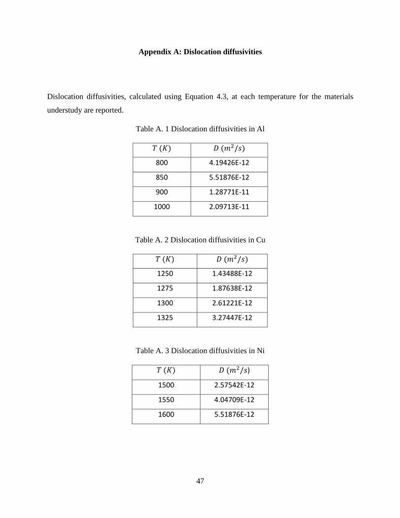
47

Appendix A: Dislocation diffusivities

Dislocation diffusivities, calculated using Equation 4.3, at each temperature for the materials

understudy are reported.

Table A. 1 Dislocation diffusivities in Al

𝑇 (𝐾) 𝐷 (𝑚2/𝑠)

800 4.19426E-12

850 5.51876E-12

900 1.28771E-11

1000 2.09713E-11

Table A. 2 Dislocation diffusivities in Cu

𝑇 (𝐾) 𝐷 (𝑚2/𝑠)

1250 1.43488E-12

1275 1.87638E-12

1300 2.61221E-12

1325 3.27447E-12

Table A. 3 Dislocation diffusivities in Ni

𝑇 (𝐾) 𝐷 (𝑚2/𝑠)

1500 2.57542E-12

1550 4.04709E-12

1600 5.51876E-12

48

Appendix B: Sample script in LAMMPS

The following script was used in LAMMPS to study the diffusion in Ni at 1550 K. The input file,

“Ni_Data.txt” contains atom IDs, coordinates of Ni atoms in a system with a relaxed screw

dislocation. Lines starting with # are comments.

units metal # define the unit system used

dimension 3 # 3 dimension simulation box

boundary f f p # boundary conditions along x, y and z directions. f for fixed

and p for periodic.

atom_style atomic # style of particles

# defining the structure, lattice parameter and orientation of x, y and z

directions

lattice fcc 3.52 orient x -1 1 -2 orient y -1 1 1 orient z 1 1 0

# reading atom IDs and coordinates from the input file

read_data Ni_Data.txt

group ni type 1

# ---------- Define Interatomic Potential ---------------------

pair_style ......................................................... eam/alloy

pair_coeff * * NiAl.eam.alloy.txt Ni # reads the EAM potential file

# ---------------fixing atoms on the edge of the cylinder-----------

region inside cylinder z 0 1 20 -25 24.8 side in units box

region edge cylinder z 0 1 20 -25 24.8 side out units box

group edge region edge

group inside region inside

fix 1 edge setforce 0 0 0

#------- defining cylinders with different radii to study diffusion -----

region diffusionR1 cylinder z 0 1 5 -25 24.8 side in units box

group diffusionR1 region diffusionR1

region diffusionR2 cylinder z 0 1 6 -25 24.8 side in units box

group diffusionR2 region diffusionR2

region diffusionR3 cylinder z 0 1 7 -25 24.8 side in units box

49

group diffusionR3 region diffusionR3

region diffusionR4 cylinder z 0 1 8 -25 24.8 side in units box

group diffusionR4 region diffusionR4

region diffusionR5 cylinder z 0 1 9 -25 24.8 side in units box

group diffusionR5 region diffusionR5

region diffusionR6 cylinder z 0 1 10 -25 24.8 side in units box

group diffusionR6 region diffusionR6

region diffusionR7 cylinder z 0 1 11 -25 24.8 side in units box

group diffusionR7 region diffusionR7

region diffusionR8 cylinder z 0 1 12 -25 24.8 side in units box

group diffusionR8 region diffusionR8

region diffusionR9 cylinder z 0 1 13 -25 24.8 side in units box

group diffusionR9 region diffusionR9

region diffusionR10 cylinder z 0 1 14 -25 24.8 side in units box

group diffusionR10 region diffusionR9

#define the timestep

reset_timestep 0

timestep 0.002

#assigning velocities to atoms with respect to the desired temperature

velocity inside create 1550 102486 mom yes rot no

# running dynamics with NVT ensemble to reach the desired temperature

fix 15 inside nvt temp 1550 1550 100

run 500000

# starting to dump output files of cylinders with different radii and run

dynamics for 30 #nanoseconds

dump 10 all custom 50000 DUMP_All_Ni_1550K.lammpstrj id type x y z

dump 11 diffusionR1 custom 10000 DUMP_R1.lammpstrj id type xu yu zu

dump 12 diffusionR2 custom 10000 DUMP_R2.lammpstrj id type xu yu zu

dump 13 diffusionR3 custom 10000 DUMP_R3.lammpstrj id type xu yu zu

dump 14 diffusionR4 custom 10000 DUMP_R4.lammpstrj id type xu yu zu

dump 15 diffusionR5 custom 10000 DUMP_R5.lammpstrj id type xu yu zu

dump 16 diffusionR6 custom 10000 DUMP_R6.lammpstrj id type xu yu zu

dump 17 diffusionR7 custom 10000 DUMP_R7.lammpstrj id type xu yu zu

dump 18 diffusionR8 custom 10000 DUMP_R8.lammpstrj id type xu yu zu

50

dump 19 diffusionR9 custom 10000 DUMP_R9.lammpstrj id type xu yu zu

run 15000000