C

Ai

Ta

b

c

h

•••••

a

ARRA

KIEHSN

1

1

smb2hco

o

0h

Journal of Neuroscience Methods 226 (2014) 88–102

Contents lists available at ScienceDirect

Journal of Neuroscience Methods

jo ur nal home p age: www.elsev ier .com/ locate / jneumeth

omputational Neuroscience

modular hierarchical approach to 3D electron microscopymage segmentation

ing Liua,b, Cory Jonesa,c, Mojtaba Seyedhosseinia,c, Tolga Tasdizena,b,c,∗

Scientific Computing and Imaging Institute, University of Utah, United StatesSchool of Computing, University of Utah, United StatesDepartment of Electrical and Computer Engineering, University of Utah, United States

i g h l i g h t s

Proposed a novel automatic hierarchical method for 2D EM image segmentation.Proposed a novel semi-automatic method for 2D EM image segmentation with minimal user intervention.Proposed a 3D linking method for 3D neuron reconstruction using 2D segmentations.Achieved close-to-human 2D segmentation accuracy.Achieved state-of-the-art 3D segmentation accuracy.

r t i c l e i n f o

rticle history:eceived 5 November 2013eceived in revised form 9 January 2014ccepted 13 January 2014

eywords:mage segmentation

a b s t r a c t

The study of neural circuit reconstruction, i.e., connectomics, is a challenging problem in neuroscience.Automated and semi-automated electron microscopy (EM) image analysis can be tremendously help-ful for connectomics research. In this paper, we propose a fully automatic approach for intra-sectionsegmentation and inter-section reconstruction of neurons using EM images. A hierarchical merge treestructure is built to represent multiple region hypotheses and supervised classification techniques areused to evaluate their potentials, based on which we resolve the merge tree with consistency constraints

lectron microscopyierarchical segmentationemi-automatic segmentationeuron reconstruction

to acquire final intra-section segmentation. Then, we use a supervised learning based linking procedurefor the inter-section neuron reconstruction. Also, we develop a semi-automatic method that utilizes theintermediate outputs of our automatic algorithm and achieves intra-segmentation with minimal userintervention. The experimental results show that our automatic method can achieve close-to-humanintra-segmentation accuracy and state-of-the-art inter-section reconstruction accuracy. We also showthat our semi-automatic method can further improve the intra-segmentation accuracy.

. Introduction

.1. Motivation

Connectomics (Sporns et al., 2005), i.e., neural circuit recon-truction, is drawing attention in neuroscience as an importantethod for studying neural circuit connectivity and the implied

ehaviors of nervous systems (Briggman et al., 2011; Bock et al.,011; Seung, 2011). It has also been shown that many diseases are

ighly related to abnormalities in neural circuitry. For instance,hanges in the neural circuitry of retina can lead to corruptionf retinal cell class circuitry, and therefore retinal degenerative

∗ Corresponding author at: Scientific Computing and Imaging Institute, Universityf Utah, Salt Lake City, UT, United States. Tel.: +1 801 581 3539.

E-mail address: tolga@sci.utah.edu (T. Tasdizen).

165-0270/$ – see front matter © 2014 Elsevier B.V. All rights reserved.ttp://dx.doi.org/10.1016/j.jneumeth.2014.01.022

© 2014 Elsevier B.V. All rights reserved.

diseases can be found by ultrastructural cell identity and circuitryexamination, which at the same time implies certain strategiesfor vision rescue (Peng et al., 2000; Marc et al., 2003, 2007, 2008;Jones et al., 2003, 2005; Jones and Marc, 2005).

To study the connectivity of a nervous system, image analy-sis techniques are widely adopted as an important approach. Forimage acquisition, electron microscopy (EM) provides sufficientlyhigh resolution on nanoscale to image not only intra-cellular struc-tures but also synapses and gap junctions, which are required forneural circuit reconstruction. In this paper, the EM images we usefor neuron segmentation and reconstruction are acquired usingserial section transmission electron microscopy (ssTEM) (Andersonet al., 2009; Chklovskii et al., 2010), serial block-face scanning elec-

tron microscopy (SBFSEM) (Denk and Horstmann, 2004), and serialsection scanning electron microscopy (ssSEM) (Horstmann et al.,2012). The use of ssTEM offers a relatively wide field of view forcell identification. However, since specimen sections have to be

cience

cirtig(urtahdwsmotciimitmfe

((mthtpaw2mrc

1

ufscAwmbntttfemlinaii

T. Liu et al. / Journal of Neuros

ut prior to imaging, thin sections are difficult to acquire, and themage volume can be very anisotropic with as high as 2 nm in-planeesolution and approximately 50 nm z-resolution. Image deforma-ions can be observed between sections to some extent even aftermage alignment, which is a challenging problem due to the ambi-uity between structure changes and coordinate transformationsTasdizen et al., 2010). These problems are to some degree avoidedsing SBFSEM, in which sections as thin as 25 nm are cut andemoved, and the remaining block face is used for imaging. Sincehe remaining block is relatively solid and stable, the section shiftsnd deformations are generally smaller than ssTEM. On the otherand, the lower intra-section resolution (about 10 nm) is a potentialrawback of SBFSEM. Recently, a novel approach based on ssSEMas introduced (Horstmann et al., 2012). This method combines

erial sectioning specimen preparation and the scanning electronicroscopy imaging technique, and is feasible to generate high res-

lution ultrastructural images of larger volumes than ssTEM. Withhe recent development of the automatic tape-collecting ultrami-rotome (ATUM), sections can be made as thin as 25 nm withoutncreasing section damage risk (Schalek et al., 2012). Another newlyntroduced imaging technique, focused ion beam scanning electron

icroscopy (FIBSEM) (Knott et al., 2008), can generate isotropicmage data with as high as 10 nm z-resolution. However, currently,he ion beam milling used for removing sections can work on a

aximum area of only 100 × 100 �m, and thus it is not feasibleor imaging substantially large tissue volumes, which is crucial toventually map the entire human brain neural connectivity.

The image datasets generated by EM are on terabyte scaleAnderson et al., 2011), and dense manual analysis can take decadesBriggman and Denk, 2006) and is thus infeasible. Therefore, auto-

atic or semi-automatic image-based connectome reconstructionechniques that can extensively reduce human workloads areighly required. Currently, fully automatic EM image segmen-ation and connectome reconstruction remain as a challengingroblem because of the complex ultrastructural cellular texturesnd the considerable variations in shape and physical topologiesithin and across image sections (Jain et al., 2007; Lucchi et al.,

010). Even though segmentation of intra-cellular structures (e.g.,itochondria, synapses) is of importance, our work focuses on neu-

on segmentation and reconstruction as a first step for automatingonnectomics.

.2. Related work

For fully automatic neuron segmentation and reconstructionsing EM images, there are two general approaches. One approachocuses on segmenting neurons in 2D images and making inter-ection linkings for 3D reconstruction, which is suggested by theurrent anisotropy of most EM image volumes except for FIBSEM.s for 2D neuron segmentation, several unsupervised attemptsere made. Anisotropic directional filtering is applied to enhanceembrane continuity (Tasdizen et al., 2005; Jurrus et al., 2008),

ut fails to detect membranes with sufficient accuracy and it can-ot remove intra-cellular structures. Kumar et al. (2010) introducedhe radon-like features to suppress undesirable intra-cellular struc-ures, but can achieve only moderate accuracy performance. Onhe other hand, supervised learning methods have proven success-ul in detecting membranes and segmenting neurons in 2D. Jaint al. (2007) trained a convolutional network to classify pixels asembrane or non-membrane. Mishchenko (2009) used a single-

ayer artificial neural network with Hessian eigenspace features todentify cell boundaries. Ciresan et al. (2012) applied deep neural

etworks (DNN) for membrane detection and achieved remark-ble results. Laptev et al. (2012) used SIFT flow to align adjacentmage sections and incorporate both intra- and inter-section pixelnformation for membrane detection. Seyedhosseini and Tasdizen

Methods 226 (2014) 88–102 89

(2013) proposed a multi-class multi-scale series contextual modelthat utilizes both cross- and inter-object information under a serialneural network framework for the detection of membranes andother cellular structures simultaneously. Given membrane detec-tion results, the classifier output can simply be thresholded (Jurruset al., 2010; Seyedhosseini et al., 2011; Ciresan et al., 2012) toacquire region segmentation. Other more sophisticated methodswere proposed to further improve the segmentation results. Kayniget al. (2010) proposed a graph-cut framework with perceptualgrouping constraints to enhance closing of membrane gaps. Liuet al. (2013) used a merge forest structure to incorporate inter-section information to improve 2D neuron segmentation. For 3Dlinking given 2D segmentation, Yang and Choe (2009) proposeda graph-cut framework to trace 2D contours in 3D. Kaynig et al.(2010) exploited geometrical consistency constraints and used theexpectation maximization algorithm to optimize the 3D affinitymatrix. Vitaladevuni and Basri (2010) considered the 3D linkingas co-clustering each pair of adjacent sections and formulated it asa quadratic optimization problem.

The other group of methods seek to achieve 2D segmentationand 3D reconstruction at the same time. Jain et al. (2011) proposeda reinforcement learning framework to merge supervoxels intosegmentations. Andres et al. (2012) proposed a graphical modelframework to incorporate both supervoxel face and boundary curveinformation for 3D supervoxel merging. Vazquez-Reina et al. (2011)generated multiple 2D segmentation hypotheses and formulatedthe 3D segmentation fusion into a Markov random field frame-work. Similarly, Funke et al. (2012) used tree structures to represent2D segmentation hypotheses and achieved 2D segmentation and3D reconstruction simultaneously by solving an integer linear pro-gramming problem with constraints. Recently, Nunez-Iglesias et al.(2013) also used an reinforcement learning framework to learna merging policy for superpixel agglomeration, which achievednotable result in isotropic FIBSEM image volume segmentation.

In addition to the automatic segmentation methods, there areseveral semi-automatic methods that utilize user input to improvesegmentation in some way. Chklovskii et al. (2010) and EyeWire(Seung, 2013) over-segment images into 2D or 3D regions, andthen let a user manually merge these regions together to formthe final cell. Post-automatic manual correction methods such asthese are sometimes called proofreading methods. Other examplesof semi-automatic segmentation include (Vazquez et al., 1998; Vuand Manjunath, 2008; Macke et al., 2008; Jurrus et al., 2009; Jeonget al., 2009), which use various input from the user to initializeautomatic methods.

The attempts to segment image volumes directly in 3D requirethe data to be close to isotropic in order to achieve acceptableresults. Although the generation of image data with isotropic res-olution becomes possible with the emergence of new EM imagingtechniques, e.g., FIBSEM (Knott et al., 2008), the image volume sizethat can be generated is currently limited. A majority of current datasets of interest are anisotropic, for which direct 3D segmentationapproaches may not be suitable.

We develop a two-step approach for 2D segmentation and 3Dreconstruction, which is suitable for both anisotropic and isotropicdata. Independent of a specific membrane detection algorithm, ourmethod takes membrane probability maps as input for superpixelgeneration, and uses a hierarchical merge tree structure to repre-sent the merging of multiple region hypotheses. We use supervisedclassification techniques to quantify the likelihoods of the hypothe-ses, based on which we acquire intra-section region segmentationvia constrained optimization or user interaction. Then we apply

a supervised learning based inter-section linking procedure for3D neuron reconstruction. We show that our automatic methodoutperforms other state-of-the-art methods and achieves close-to-human errors in terms of 2D segmentation and state-of-the-art 3D

9 cience

rmibnoomtf

2

etaaasai

2

ascwC

itf

T

T

F

F

wilpTagcuppe

itu

image by simply thresholding the probability map. With thisapproach, however, a few false negatives can cause significantunder-segmentation errors. To address this problem, we propose a

0 T. Liu et al. / Journal of Neuros

econstruction accuracy. We also show that our semi-automaticethod can further improve the 2D segmentation result with min-

mal user intervention. Compared with the other most recent worky Nunez-Iglesias et al. (2013), it is noteworthy that the use ofode potential in our method (see Section 2.2.5) utilizes higherrder information to make merging decisions than only thresh-lding boundary classifier output. Also, our merge tree frameworkakes it convenient to incorporate prior knowledge about segmen-

ation, which is not easily achievable in the reinforcement learningramework (Nunez-Iglesias et al., 2013).

. Methods

Let X = {xi} be an input image. A segmentation S = {si} assignsach pixel an integer label that is unique for each object. A groundruth segmentation G = {gi} is usually generated by human expertsnd is considered as the gold standard. This notation applies torbitrarily dimensional images. In this paper, we refer to a 2D images an image or a section, and a sequence of 2D images as an imagetack. The accuracy of a segmentation S is measured based on itsgreement with the ground truth G. The measurement of agreements introduced in Section 2.1.

.1. Segmentation accuracy metric

For both purposes of learning and evaluating the segmentation, metric that is sensitive to correct region separation but less sen-itive to minor shifts in the boundaries is desired. Traditional pixellassification error metrics are not effective in this regard. Instead,e chose to use the modified Rand error metric from the ISBI EMhallenge (Arganda-Carreras et al., 2012, 2013).

The adapted Rand error is based on the pairwise pixel metricntroduced by Rand (1971). For both the original Rand index andhe adapted Rand error, the true positives (TP), true negatives (TN),alse positives (FP) and false negatives (FN) are computed as:

P =∑

i

∑j>i

�(

si = sj ∧ gi = gj

), (1)

N =∑

i

∑j>i

�(

si /= sj ∧ gi /= gj

), (2)

P =∑

i

∑j>i

�(

si = sj ∧ gi /= gj

), (3)

N =∑

i

∑j>i

�(

si /= sj ∧ gi = gj

), (4)

here �(·) is a function that returns 1 if the argument is true and 0f the argument is false. Each of these calculations compares theabels of a given pixel pair in S, (si, sj), with the correspondingixel pair in G, (gi, gj), for all possible pixel pairs in the image.P, which counts the number of pixels for which si = sj and gi = gj,nd TN, which counts the number of pixels for which si /= sj andi /= gj, correspond to accurately segmented pixel pairs. FP, whichounts the number of pixels which si = sj but gi /= gj, corresponds tonder-segmented pixel pairs, and FN, which counts the number ofixels for which si /= sj but gi = gj, corresponds to over-segmentedixel pairs. These pairs are considered across a single image for 2Dvaluation and across a full image stack for 3D evaluation.

In the original Rand index, the metric is computed by divid-ng the number of true pairs both positive and negative by theotal number of possible pairs in the image. This results in val-es between 0 and 1 with 1 being an indication of a perfect

Methods 226 (2014) 88–102

segmentation. The adapted Rand error, however, is 1 minus the F-score computed from these results using precision and recall where

Precision = TP

TP + FP, (5)

Recall = TP

TP + FN, (6)

F-score = 2 × Precision × RecallPrecision + Recall

, (7)

Adapted Rand error = 1 − F-score. (8)

Once again the values of the adapted Rand error are between 0 and1, but with 0 now representing a perfect segmentation.

One advantage of using this metric is that when the erroris high, the precision and recall provide additional informationregarding the type of error that is present. When precision ishigh and recall is low, this is an indication that the imagehas been more over-segmented. Conversely if recall is high andprecision is low, the indication is that the image is under-segmented resulting from regions being merged that shouldhave been separate. Errors such as boundaries between regionsbeing in the shifted locations or a mix of under- and over-segmentations will result in a more balanced value for precisionand recall.

This metric is particularly useful in segmentation of EM imagesbecause it can be computed accurately independent of the num-ber of regions segmented. One implementation consideration forour application is that all pixels where gi corresponds to boundarypixels are ignored. The reason for excluding these pixels is that ifthe proposed region entirely encompasses the ground truth regionand the boundary between regions falls within the true boundary,then the segmentation is accurate for the purposes of this applica-tion.

2.2. Intra-section segmentation1

In this section, we propose a fully automatic method for 2D EMimage segmentation. We take a membrane detection probabilitymap as input and transform it into an initial segmentation usingthe watershed algorithm. Then starting with the initial segmen-tation, we use an iterative algorithm to build the merge tree as arepresentation of region merging hierarchy. Non-local features arecomputed and a boundary classifier is trained to give predictionsabout region merging, based on which we assign a node potentialto each node in the merge tree. We resolve the merge tree using agreedy optimization approach under a pixel consistency constraintand generate the final segmentation. Furthermore, we present asemi-automatic merge tree resolution approach to improve thesegmentation accuracy while minimizing the user time consump-tion.

2.2.1. Pixel-wise membrane detectionOur intra-section segmentation method uses pixel-wise mem-

brane detection probability maps as input. A membrane detectionmap B = {bi} is a probability image with each pixel intensity bi ∈ [0,1] as shown in Fig. 1b. Such membrane detection maps are com-monly obtained using machine learning algorithms, such as (Jainet al., 2007; Laptev et al., 2012; Ciresan et al., 2012; Seyedhosseiniet al., 2013). We can obtain a segmentation of the cells in the

1 The preliminary version of the fully automatic method was presented in ICPR2012 (Liu et al., 2012).

T. Liu et al. / Journal of Neuroscience Methods 226 (2014) 88–102 91

Fig. 1. Example of (a) an original EM image, (b) a membrane detection probability map, and (c) an initial segmentation. Each connected component in the initial segmentationi sult in

rpot((co

2

msafbpHAm2TeocrdcbtrbtwbbAar

2

iwbp

ing only two regions. In determining the merging saliency, we findthat the membrane detection probability performs more accuratelyand consistently than the original image intensity. As an example

s considered as an initial region. Some boundaries that are too faint to see in (b) re

egion-based method for 2D segmentation. Our method is inde-endent of how the membrane detection probability maps arebtained. In Section 3, we experiment with the membrane detec-ion probability maps learned with cascaded hierarchical modelsCHM) (Seyedhosseini et al., 2013) and deep neural networks (DNN)Ciresan et al., 2012), and we show that our method can signifi-antly improve the segmentation accuracy over thresholding eitherf these probability maps.

.2.2. Initial segmentationBased on the probability maps, we generate an initial seg-

entation for each image, which over-segments the image intouperpixels. It is important to use the membrane detection prob-bility maps instead of the original intensity images, because theormer usually removes intra-cellular structures and preserves celloundaries. Many methods can be applied to generate the super-ixel initial segmentation (Shi and Malik, 2000; Felzenszwalb anduttenlocher, 2004; Levinshtein et al., 2009; Veksler et al., 2010;chanta et al., 2012). Our method uses, but is not limited to, theorphological watershed implementation (Beare and Lehmann,

006) provided in the Insight Segmentation and Registrationoolkit (ITK) (Yoo et al., 2002), because of its high computationalfficiency and good adherence to image boundaries. The basic ideaf the watershed algorithm (Beucher and Lantuejoul, 1979) is toonsider an image as a 3D terrain map with pixel intensities rep-esenting heights. As the rain falls into the terrain, water flowsown along the steepest path and forms lakes in the basins, whichorrespond to regions or segments of the image, and the bordersetween lakes are called watershed lines. In terms of implemen-ation, local minima of the image are used as seeds, from whichegions are grown based on intensity gradients until the regionoundaries touch. Fig. 1 shows an example of an initial segmen-ation. In practice, we blur the membrane detection probabilitiesith a Gaussian filter and ignore the local minima with dynamics

elow threshold tw to avoid too many initial regions. Meanwhile,y using a small value of tw , we can ensure over-segmentation.lso, we keep the one-pixel wide watershed lines as background,nd use these points as boundary points between foregroundegions.

.2.3. Merge tree constructionGiven a set of disjoint regions R = {ri}, in which each region ri

s a point set, and the background point set (watershed lines) rb,e define the boundary between two regions ri and rj as a set of

ackground points that are in the 4-connected neighborhoods ofoints from both of the two regions, respectively:

regions since we aim for an initial over-segmentation.

boundary(ri, rj)={p ∈ rb | ∃pi′ ∈ ri, pj′ ∈ rj, s.t.p ∈ N4(pi′ ) ∩ N4(pj′ )},(9)

where N4(·) represents the set of 4-connected neighbor points ofa given point. If boundary(ri, rj) is not the empty set, we say thatregion ri and rj are neighbors. Next, we define a merge of m regions{r1, r2, . . ., rm} as the union of these region point sets as well as theset of boundary points between these regions:

merge(r1, r2, . . ., rm)

=(⋃m

i=1ri

)∪

(⋃m−1

i=1

⋃m

j=i+1boundary(ri, rj)

). (10)

Notice that merge(r1, r2, . . ., rm) is also a region. As an exampleshown in Fig. 2, region ri and rj merge to form region rk, which con-sists of the points from both region ri and rj and also the boundarypoints between them. Next, we define a merging saliency func-tion fX,B : Rm → R, which takes a set of m regions and uses thepixel information from the original image and/or the membranedetection probability map to determine the merging saliency ofthe regions, which is a real number. Larger saliency indicates theregions are more likely to merge. In practice, we consider merg-

Fig. 2. Example of region merging. (a) Two merging regions ri and rj (green) and theirboundary (magenta), and (b) the merging result region rk (blue) are overlaid to theground truth segmentation. The boundary is dilated for visualization purposes. (Forinterpretation of the references to color in this figure legend, the reader is referredto the web version of this article.)

9 cience

sltabatbasi

f

ttintcbt

bmwlAoaaartilt1r

r{sjTm

(

taapr

2

pishatt

2 T. Liu et al. / Journal of Neuros

hown in Fig. 1, some intra-cellular structures, e.g., mitochondria,ook even darker than the membranes in the original image, andhus using these original intensities could give false indicationsbout region merging saliency. In the membrane detection proba-ility map, however, the strengths of such pixels are suppressednd the membrane pixels are distinguished. Also, we find thathe median of the membrane probabilities of the boundary pointsetween two regions is a good indication of region merging saliencynd gives a more robust boundary measure than other statistics,uch as minimum and mean. Thus, the merging saliency functions specified as

B(ri, rj) = 1 − median({bp ∈ B | p ∈ boundary(ri, rj)}). (11)

In practice, some regions in the initial segmentation could beoo small to extract meaningful region-based features (see Sec-ion 2.2.4), so we optionally conduct a pre-merging step to mergenitial regions smaller than a certain threshold ta1 pixels to one of itseighbor regions that yields the largest merging saliency accordingo Eq. (11). We also pre-merge a region if its size is smaller than aertain threshold ta2 pixels and its average intensity from the mem-rane detection probability map of all its pixels is above a certainhreshold tp.

To represent the hierarchy of region merging, we use a fullinary tree structure T = (N, E), which we call a merge tree. In aerge tree, node nd

i∈ N represents a region ri ∈ R in the image,

here d denotes the depth in the tree at which this node occurs. Theeaf nodes represent the regions from the initial over-segmentation.

non-leaf node corresponds to a region that is formed by oner more merges; the root node corresponds to the whole images one single region. An undirected edge eij ∈ E between node nind its parent node nj means region ri is a subregion of region rj,nd a local structure ({nd

j, nd+1

i1, nd+1

i2}, {ei1j, ei2j}) represents region

j is the merging result of region ri1 and ri2 . Fig. 3 shows a mergeree example with the corresponding initial segmentation shownn Fig. 3a. Fourteen initial regions (region 1–14) correspond to theeaf nodes in the merge tree (node 1–14). The non-leaf nodes arehe merging result of their descendant regions. For example, region5 is the merging result of region 4 and 10. The root node 27 cor-esponds to the whole image.

To construct a merge tree, we start with the initialegions R = {r1, r2, . . ., rN0 }, the corresponding leaf nodes N =nd1

1 , nd22 , . . ., ndN0N0

}, and an empty edge set E. First, we extract theet of all region pairs that are neighbors, P = {(ri, rj) ∈ R × R | i <, rj ∈ NR(ri)}, where NR(ri) denotes the neighbor region set of ri.hen we pick the region pair (ri∗ , rj∗ ) from P that yields the largesterging saliency function output as

ri∗ , rj∗ ) = arg max(ri,rj)∈P

fB(ri, rj). (12)

Let rk be the merging result of ri∗ and rj∗ . A node nk correspondingo rk is added as the parent of node ni∗ and nj∗ into N and edges ei∗k

nd ej∗k are added to E. Meanwhile, we append R with rk, removeny region pair related to ri∗ or rj∗ from P, and add all the regionairs concerning rk into P. This process is repeated until there is noegion pair left in P, and T = (N, E) is the merge tree.

.2.4. Boundary classifierIn a merge tree, each non-leaf node and its children represent a

otential region merging ({ndk, nd+1

i, nd+1

j}, {eik, ejk}), the probabil-

ty of which is needed for selecting the best segments. One possibleolution is to use the merging saliency function output, which,

owever, relies only on the boundary cues, and cannot utilize thebundant information from the two merging regions. Instead, werain a boundary classifier to give such predictions by outputtinghe probability of region merging. The boundary classifier takes 88

Methods 226 (2014) 88–102

non-local features computed from each pair of merging regions,including region geometry, image intensity, and texture statisticsfrom both original EM images and membrane detection probabil-ity maps, and merging saliency information (see Appendix B for asummary of features). One advantage of our features over the localfeatures commonly used by pixel classifiers (Laptev et al., 2012;Seyedhosseini et al., 2013) is that our features are extracted fromregions instead of pixels and thus can be more informative. Forinstance, we use geometric features to incorporate region shapeinformation for the classification procedure, which is not feasiblefor pixel classifiers.

To generate training labels that indicate whether the boundarybetween two regions exists or not, we utilize the ground truth seg-mentation of the training data. As shown in Fig. 2, when decidingwhether region ri and region rj should merge to become regionrk, we compute the adapted Rand errors (see Section 2.1) for bothmerging (εk) and keeping split (εij) against the ground truth. Eithercase with smaller error deviates less from the ground truth andshould thus be adopted. Therefore, the training label is determinedautomatically as

yij→k ={

+1(boundary exists, not merge) ifεij ≤ εk

−1(boundary not exist, merge) otherwise.(13)

The boundary classifier is not limited to a specific supervisedclassification model. We choose the random forest (Breiman, 2001)among various other classifiers because of its fast training andremarkable performance. Different weights are assigned to posi-tive/negative samples to balance their contributions to the trainingprocess. The weights for positive sample wpos and for negative sam-ples wneg are determined as

wpos ={

Nneg/Npos if Npos < Nneg

1 otherwise, (14)

wneg ={

Npos/Nneg if Npos > Nneg

1 otherwise, (15)

where Npos and Nneg are the number of samples with positive andnegative labels, respectively.

2.2.5. Automatic merge tree resolutionAfter creating the merge tree, the task of generating a final seg-

mentation of the image becomes choosing a subset of nodes in themerge tree. The boundary classifier predicts the probability for eachpotential merge, based on which we define a local potential for eachnode that represents the likelihood that it is a correct segmentation.Considering (a) a region exists in the final segmentation because itneither splits into smaller regions nor merges into others and (b)each prediction the boundary classifier makes depends only on thelocal merge tree structure, we define the potential for a node nd

ias

Pi = pic1 ,ic2 →i · (1 − pi,is→ip ), (16)

where pic1 ,ic2 →i is the probability that the child nd+1ic1

and nd+1ic2

merge

to node ndi, and pi,is→ip is the probability that node nd

imerges with

its sibling ndis

to the parent nd−1ip

. Both of these probabilities come

from the boundary classifier. As an example shown in Fig. 3, thepotential of node 24 is P24 = p20,21→24(1 − p2,24→26). Since there areno children for a leaf node, its potential is computed as the squareof 1 minus the probability that it merges with its sibling. Similarly,

the potential of the root node is the square of the probability thatits children merge.

Given the node potentials, we would like to choose a subsetof nodes in the merge tree that have high potentials and preserve

T. Liu et al. / Journal of Neuroscience Methods 226 (2014) 88–102 93

Fig. 3. Example of (a) an initial segmentation, (b) a consistent final segmentation, both overlaid with an original EM image, and (c) a corresponding merge tree. The leaf nodesh ons inS erge

b s refer

trslCtowlnTpaad

mwactc

2

stsmosuti

ave identical labels as the initial regions, and the colored nodes correspond to regiection 2.2.5, the potential of node 24 equals the probability that node 20 and 21 mox). (For interpretation of the references to color in this figure legend, the reader i

he pixel consistency of the final segmentation. Pixel consistencyequires that any pixel should have exactly one label in the finalegmentation, either a background label or one of the foregroundabels, each of which is assigned to a unique connected component.onsequently, if a node in the merge tree is chosen, all of its ances-ors and descendants cannot be selected; if a node is not chosen, onef its ancestors or a set of its descendants must be selected. In otherords, exactly one node should be selected on the path from every

eaf node to the root node. Fig. 3 shows an example: the coloredodes are picked to form a consistent final segmentation in Fig. 3.he other nodes cannot be picked, because we cannot label anyixel more than once. For example, if node 4 (or 10) is also pickedlong with node 15, the pixels in region 4 (or 10) would be labeleds both 15 and 4 (or 10), which violates the pixel consistency byefinition.

Under the pixel consistency constraint, we use a greedy opti-ization approach to resolve the merge tree. First, we pick the nodeith the highest potential in the merge tree. Then the ancestors

nd descendants of the picked node are removed as inconsistenthoices. This procedure is repeated until every node in the mergeree is either picked or removed. The set of picked nodes form aonsistent 2D segmentation.

.2.6. Semi-automatic merge tree resolutionOn each of the data sets we have applied the automatic intra-

ection segmentation method to, the improvement over optimallyhresholding the automatic intra-section segmentation has beenignificant. Depending on the data set, however, the final seg-entation may not be sufficiently accurate for the application. To

vercome situations where the resulting accuracy for a given data

et is insufficient, we also developed a method for allowing man-al input in resolving the merge tree. The goal with this method iso minimize the time requirement of the manual input while stillmproving the accuracy of the final result.

the final segmentation. As an example of node potential computation described into node 24 (the green box), while node 2 and 24 do not merge to node 26 (the redred to the web version of this article.)

Using the Visualization Toolkit (Schroeder et al., 2006), wepresent the user with an image of the original image overlaid withthe proposed segmentation. The user will then be presented withan unresolved region with the highest node potential in the mergetree, and specify whether it is good, over-segmented (if the regionis too small), under-segmented (if the region is too large), or poorlysegmented (if the region contains portions of multiple regions, butno complete region). Fig. 4 shows what the interface (Fig. 4a) andeach segmentation possibility (Figs. 4b–4e) look like.

If the region is specified as good, the region is labeled in the labelimage and the ancestors and descendants are removed from themerge tree as described previously. The next region presented tothe user follows the greedy approach as described in Section 2.2.5.Ideally this will be the dominant answer and it will take minimaltime for the user to resolve the tree.

If the region is instead specified as either under-segmentedor over-segmented, the proper portions of the tree are removedand the next region is presented according to this pick. When itis over-segmented, the descendants are removed and the parentis presented as the next region; when it is under-segmented, theancestors are removed and the highest potential child is presentedas the next region. Doing this allows the user to immediately resolveeach region which will require less time than having to revisit andre-examine the region. If the parent in the case of over-segmentedor the children in the case of under-segmented have already beenremoved from the tree structure, then the assumption of the cor-rect segmentation of this region being in the tree fails and the nextnode presented once again follows the same greedy approach asabove.

Finally, if the region is specified as bad, this is an indication thatthe correct segmentation for this region is not present in the tree.

The ancestors and descendants along with the region presentedare all removed from the tree and the next region presented willagain follow the greedy approach. This will lead to some regionsof the image being left unresolved. To accommodate this scenario,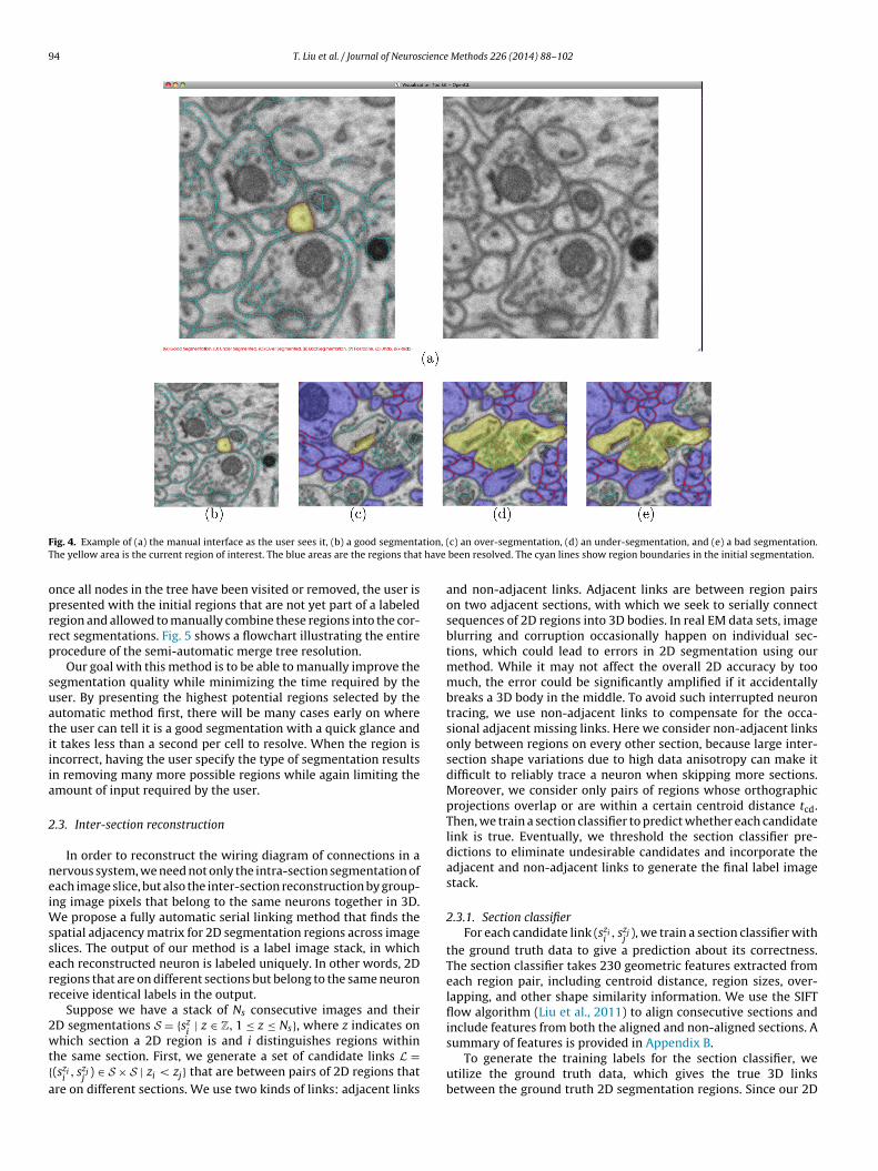

94 T. Liu et al. / Journal of Neuroscience Methods 226 (2014) 88–102

F tion, (T have

oprrp

suatiiia

2

neiWsserr

2wt{a

ig. 4. Example of (a) the manual interface as the user sees it, (b) a good segmentahe yellow area is the current region of interest. The blue areas are the regions that

nce all nodes in the tree have been visited or removed, the user isresented with the initial regions that are not yet part of a labeledegion and allowed to manually combine these regions into the cor-ect segmentations. Fig. 5 shows a flowchart illustrating the entirerocedure of the semi-automatic merge tree resolution.

Our goal with this method is to be able to manually improve theegmentation quality while minimizing the time required by theser. By presenting the highest potential regions selected by theutomatic method first, there will be many cases early on wherehe user can tell it is a good segmentation with a quick glance andt takes less than a second per cell to resolve. When the region isncorrect, having the user specify the type of segmentation resultsn removing many more possible regions while again limiting themount of input required by the user.

.3. Inter-section reconstruction

In order to reconstruct the wiring diagram of connections in aervous system, we need not only the intra-section segmentation ofach image slice, but also the inter-section reconstruction by group-ng image pixels that belong to the same neurons together in 3D.

e propose a fully automatic serial linking method that finds thepatial adjacency matrix for 2D segmentation regions across imagelices. The output of our method is a label image stack, in whichach reconstructed neuron is labeled uniquely. In other words, 2Degions that are on different sections but belong to the same neuroneceive identical labels in the output.

Suppose we have a stack of Ns consecutive images and theirD segmentations S = {sz

i| z ∈ Z, 1 ≤ z ≤ Ns}, where z indicates on

hich section a 2D region is and i distinguishes regions withinhe same section. First, we generate a set of candidate links L =(szi

i, szj

j) ∈ S × S | zi < zj} that are between pairs of 2D regions that

re on different sections. We use two kinds of links: adjacent links

c) an over-segmentation, (d) an under-segmentation, and (e) a bad segmentation.been resolved. The cyan lines show region boundaries in the initial segmentation.

and non-adjacent links. Adjacent links are between region pairson two adjacent sections, with which we seek to serially connectsequences of 2D regions into 3D bodies. In real EM data sets, imageblurring and corruption occasionally happen on individual sec-tions, which could lead to errors in 2D segmentation using ourmethod. While it may not affect the overall 2D accuracy by toomuch, the error could be significantly amplified if it accidentallybreaks a 3D body in the middle. To avoid such interrupted neurontracing, we use non-adjacent links to compensate for the occa-sional adjacent missing links. Here we consider non-adjacent linksonly between regions on every other section, because large inter-section shape variations due to high data anisotropy can make itdifficult to reliably trace a neuron when skipping more sections.Moreover, we consider only pairs of regions whose orthographicprojections overlap or are within a certain centroid distance tcd.Then, we train a section classifier to predict whether each candidatelink is true. Eventually, we threshold the section classifier pre-dictions to eliminate undesirable candidates and incorporate theadjacent and non-adjacent links to generate the final label imagestack.

2.3.1. Section classifierFor each candidate link (szi

i, szj

j), we train a section classifier with

the ground truth data to give a prediction about its correctness.The section classifier takes 230 geometric features extracted fromeach region pair, including centroid distance, region sizes, over-lapping, and other shape similarity information. We use the SIFTflow algorithm (Liu et al., 2011) to align consecutive sections andinclude features from both the aligned and non-aligned sections. A

summary of features is provided in Appendix B.

To generate the training labels for the section classifier, weutilize the ground truth data, which gives the true 3D linksbetween the ground truth 2D segmentation regions. Since our 2D

T. Liu et al. / Journal of Neuroscience Methods 226 (2014) 88–102 95

matic

ssstsctgpuits

cbot

Fig. 5. Flowchart of the semi-auto

egmentation does not match the ground truth perfectly, each 2Degmentation region is matched to one ground truth region thathares the largest overlapping area. Then all the links betweenhe ground truth regions that have at least one corresponding 2Degmentation region are regarded as the true links. All the otherandidate links are considered as false links. Note that it is impor-ant to use the training 2D segmentation results instead of theround truth 2D segmentations to generate the training link sam-les for the section classifier, because the training link samplessing the training 2D segmentation results resemble better the test-

ng data than those using the ground truth 2D segmentation andhus the section classifier can be better generalized for the testingamples.

We choose the random forest algorithm (Breiman, 2001) as the

lassifier. The training data can be very imbalanced, since there cane several candidate links from any given region but usually onlyne or two of them are true. Therefore, it is important to balancehe training process by assigning different weights according to Eqs.

merge tree resolution procedure.

(14) and (15). Two separate classifiers are trained for the adjacentand non-adjacent links, respectively.

2.3.2. LinkingWe use the output probability for each candidate link as a weight

and apply a thresholding strategy to preserve the most reliable linksand remove all other candidates. We use a threshold tadj for adja-cent links and a separate threshold tnadj for non-adjacent links. Fora 2D segmentation region sz

i, in the forward directions of z, we pick

the adjacent links (szi, sz+1

j′ ) whose weights are above tadj, and ifthere is no adjacent link picked for sz

i, we pick the non-adjacent

links (szi, sz+2

j′ ) whose weights are above tnadj. Similarly, in the back-

ward direction, the adjacent links (sz−1k

, szi) with weights above tadj

are picked, and if there are no such links for szi, we pick the non-

adjacent links (sz−2k′ , sz

i) with weights above tnadj. Finally, we force

one candidate adjacent link with the largest weight to be preservedfor every region without any picked links, on the grounds that the

96 T. Liu et al. / Journal of Neuroscience

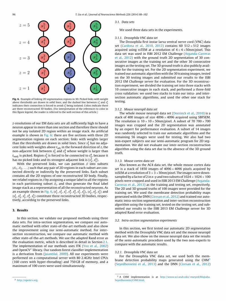
Fig. 6. Example of linking 2D segmentation regions in 3D. Picked links with weightabove thresholds are drawn in solid lines, and the dashed line between s3

3 and s43

indicates their connection is forced to avoid s3 being isolated. Colors indicate thereat

znnestcnth

{ncwiia{t

3

dmtsotTaip(m

For the Drosophila VNC data set, we used both the mem-

3re three reconstructed 3D bodies. (For interpretation of the references to color inhis figure legend, the reader is referred to the web version of this article.)

-resolutions of our EM data sets are all sufficiently high to have aeuron appear in more than one section and therefore there shouldot be any isolated 2D region within an image stack. An artificialxample is shown in Fig. 6: there are five sections with three 2Degmentation regions on each section; links with weights largerhan the thresholds are drawn in solid lines. Since s2

3 has no adja-ent links with weights above tadj in the forward direction of z, theon-adjacent link between s2

3 and s43 whose weight is larger than

nadj is picked. Region s33 is forced to be connected to s4

3, because itas no picked links and its strongest adjacent link is (s3

3, s43).

With the preserved links, we can partition S into subsetsS1, S2, . . .} such that any pair of 2D regions in each subset are con-ected directly or indirectly by the preserved links. Each subsetontains all the 2D regions of one reconstructed 3D body. Finally,e relabel regions in S by assigning a unique label to all the regions

n each partitioning subset Si, and thus generate the final labelmage stack as a representation of all the reconstructed neurons. Asn example shown in Fig. 6, {s1

1, s21, s3

1, s41, s4

2, s51, s5

2}, {s12, s2

2, s32} and

s13, s2

3, s33, s4

3, s53} constitute three reconstructed 3D bodies, respec-

ively, according to the preserved links.

. Results

In this section, we validate our proposed methods using threeata sets. For intra-section segmentation, we compare our auto-atic method with other state-of-the-art methods and also show

he improvement using our semi-automatic method. For inter-ection reconstruction, we compare our automatic method withther state-of-the-art methods. We use the adapted Rand error ashe evaluation metric, which is described in detail in Section 2.1.he implementation of our methods uses ITK (Yoo et al., 2002)nd OpenCV2 library. Our random forest classifier implementations a derivation from (Jaiantilal, 2009). All our experiments were

erformed on a computational server with 80 2.4GHz Intel CPUs160 cores with hyper-threading) and 750 GB of memory, and a

aximum of 100 cores were used simultaneously.

2 http://opencv.org.

Methods 226 (2014) 88–102

3.1. Data sets

We used three data sets in the experiments.

3.1.1. Drosophila VNC data setThe Drosophila first instar larva ventral nerve cord (VNC) data

set (Cardona et al., 2010, 2012) contains 60 512 × 512 imagesacquired using ssTEM at a resolution of 4 × 4 ×50nm/pixel. Thisdata set was used in ISBI 2012 EM Challenge (Arganda-Carreraset al., 2012) with the ground truth 2D segmentation of 30 con-secutive images as the training set and the other 30 consecutiveimages as the testing set. The 3D ground truth is also publicly avail-able for the training set. For the 2D segmentation experiment, wetrained our automatic algorithm with the 30 training images, testedon the 30 testing images and submitted our results to the ISBI2012 EM Challenge server for evaluation. For the 3D reconstruc-tion experiment, we divided the training set into three stacks with10 consecutive images in each stack, and performed a three-foldcross validation: we used two stacks to train our intra- and inter-section automatic algorithms, and used the other one stack fortesting.

3.1.2. Mouse neuropil data setThe whole mouse neuropil data set (Deerinck et al., 2010) is a

stack of 400 images of size 4096 × 4096 acquired using SBFSEM.The resolution is 10 × 10 × 50nm/pixel. A subset of 70 700 × 700images was cropped and the 2D segmentation was annotatedby an expert for performance evaluation. A subset of 14 imageswas randomly selected to train our automatic algorithms and theremaining 56 images were used for testing. We also had twonon-expert subjects use our semi-automatic program for 2D seg-mentation. We did not evaluate our inter-section reconstructionalgorithm using the data set due to the absence of the 3D groundtruth.

3.1.3. Mouse cortex data setAlso known as the AC4 data set, the whole mouse cortex data

set is a stack of 1850 images of 4096 × 4096 pixels acquired byssSEM at a resolution of 3 × 3 ×30nm/pixel. The images were down-sampled by a factor of 2 in x–y and two subsets of 1024 × 1024 × 100pixels were cropped and used in ISBI 2013 EM Challenge (Arganda-Carreras et al., 2013) as the training and testing set, respectively.The 2D and 3D ground truths of 100 images were provided for thetraining set. We used the membrane detection probability mapsgenerated with the DNN (Ciresan et al., 2012) and trained our auto-matic intra-section segmentation and inter-section reconstructionalgorithm using the training set, tested on the testing set, and sub-mitted our results to the ISBI 2013 EM Challenge server for 3Dadapted Rand error evaluation.

3.2. Intra-section segmentation experiments

In this section, we first tested our automatic 2D segmentationmethod with the Drosophila VNC data set and the mouse neuropildata set. We also show on the mouse neuropil data set the resultsof the semi-automatic procedure used by the two non-experts tocompare with the automatic results.

3.2.1. Drosophila VNC data set

brane detection probability maps generated using the CHM3

(Seyedhosseini et al., 2013) and the DNN (Ciresan et al., 2012)

3 A CHM implementation is at http://www.sci.utah.edu/ mseyed/MojtabaSeyedhosseini/CHM.html.

T. Liu et al. / Journal of Neuroscience Methods 226 (2014) 88–102 97

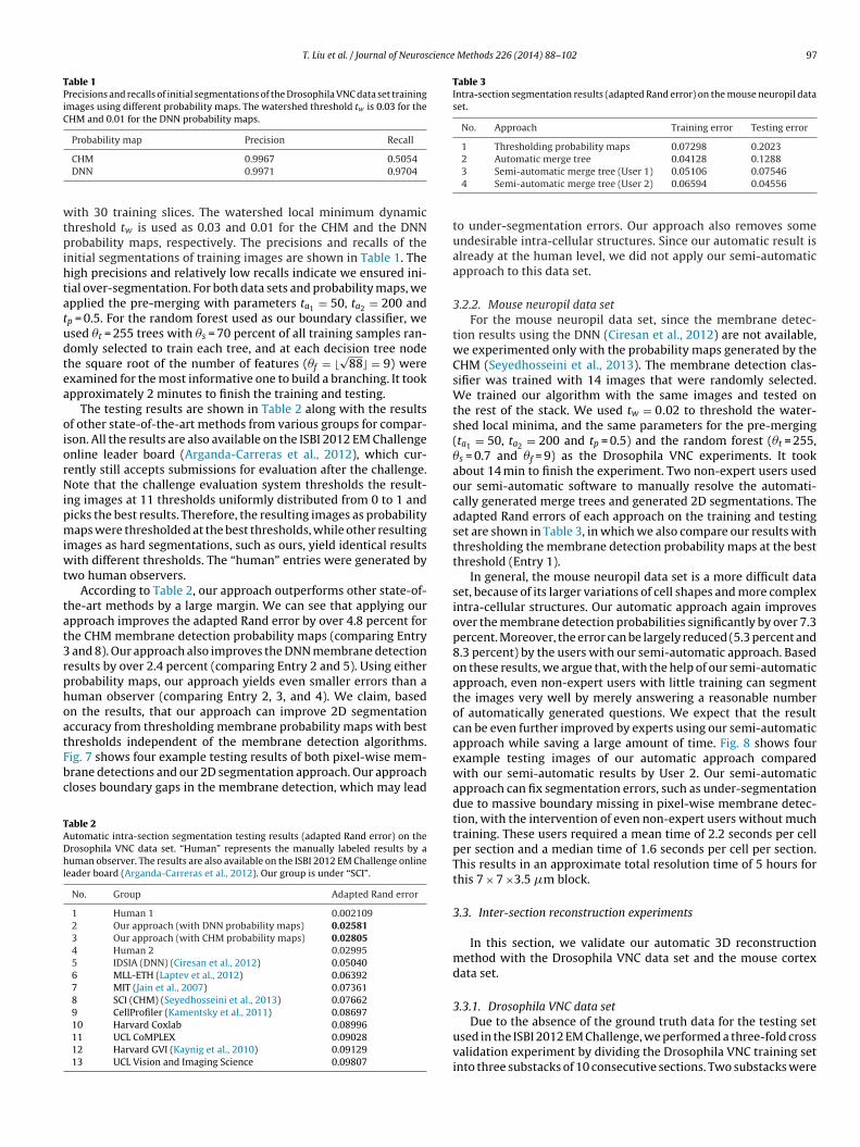
Table 1Precisions and recalls of initial segmentations of the Drosophila VNC data set trainingimages using different probability maps. The watershed threshold tw is 0.03 for theCHM and 0.01 for the DNN probability maps.

Probability map Precision Recall

wtpihtatudtea

oiorNipmiwt

tat3rphoatFbc

TADhl

Table 3Intra-section segmentation results (adapted Rand error) on the mouse neuropil dataset.

No. Approach Training error Testing error

1 Thresholding probability maps 0.07298 0.20232 Automatic merge tree 0.04128 0.1288

CHM 0.9967 0.5054

DNN 0.9971 0.9704

ith 30 training slices. The watershed local minimum dynamichreshold tw is used as 0.03 and 0.01 for the CHM and the DNNrobability maps, respectively. The precisions and recalls of the

nitial segmentations of training images are shown in Table 1. Theigh precisions and relatively low recalls indicate we ensured ini-ial over-segmentation. For both data sets and probability maps, wepplied the pre-merging with parameters ta1 = 50, ta2 = 200 andp = 0.5. For the random forest used as our boundary classifier, wesed �t = 255 trees with �s = 70 percent of all training samples ran-omly selected to train each tree, and at each decision tree nodehe square root of the number of features (�f = �

√88 = 9) were

xamined for the most informative one to build a branching. It tookpproximately 2 minutes to finish the training and testing.

The testing results are shown in Table 2 along with the resultsf other state-of-the-art methods from various groups for compar-son. All the results are also available on the ISBI 2012 EM Challengenline leader board (Arganda-Carreras et al., 2012), which cur-ently still accepts submissions for evaluation after the challenge.ote that the challenge evaluation system thresholds the result-

ng images at 11 thresholds uniformly distributed from 0 to 1 andicks the best results. Therefore, the resulting images as probabilityaps were thresholded at the best thresholds, while other resulting

mages as hard segmentations, such as ours, yield identical resultsith different thresholds. The “human” entries were generated by

wo human observers.According to Table 2, our approach outperforms other state-of-

he-art methods by a large margin. We can see that applying ourpproach improves the adapted Rand error by over 4.8 percent forhe CHM membrane detection probability maps (comparing Entry

and 8). Our approach also improves the DNN membrane detectionesults by over 2.4 percent (comparing Entry 2 and 5). Using eitherrobability maps, our approach yields even smaller errors than auman observer (comparing Entry 2, 3, and 4). We claim, basedn the results, that our approach can improve 2D segmentationccuracy from thresholding membrane probability maps with best

hresholds independent of the membrane detection algorithms.ig. 7 shows four example testing results of both pixel-wise mem-rane detections and our 2D segmentation approach. Our approachloses boundary gaps in the membrane detection, which may lead

able 2utomatic intra-section segmentation testing results (adapted Rand error) on therosophila VNC data set. “Human” represents the manually labeled results by auman observer. The results are also available on the ISBI 2012 EM Challenge online

eader board (Arganda-Carreras et al., 2012). Our group is under “SCI”.

No. Group Adapted Rand error

1 Human 1 0.0021092 Our approach (with DNN probability maps) 0.025813 Our approach (with CHM probability maps) 0.028054 Human 2 0.029955 IDSIA (DNN) (Ciresan et al., 2012) 0.050406 MLL-ETH (Laptev et al., 2012) 0.063927 MIT (Jain et al., 2007) 0.073618 SCI (CHM) (Seyedhosseini et al., 2013) 0.076629 CellProfiler (Kamentsky et al., 2011) 0.0869710 Harvard Coxlab 0.0899611 UCL CoMPLEX 0.0902812 Harvard GVI (Kaynig et al., 2010) 0.0912913 UCL Vision and Imaging Science 0.09807

3 Semi-automatic merge tree (User 1) 0.05106 0.075464 Semi-automatic merge tree (User 2) 0.06594 0.04556

to under-segmentation errors. Our approach also removes someundesirable intra-cellular structures. Since our automatic result isalready at the human level, we did not apply our semi-automaticapproach to this data set.

3.2.2. Mouse neuropil data setFor the mouse neuropil data set, since the membrane detec-

tion results using the DNN (Ciresan et al., 2012) are not available,we experimented only with the probability maps generated by theCHM (Seyedhosseini et al., 2013). The membrane detection clas-sifier was trained with 14 images that were randomly selected.We trained our algorithm with the same images and tested onthe rest of the stack. We used tw = 0.02 to threshold the water-shed local minima, and the same parameters for the pre-merging(ta1 = 50, ta2 = 200 and tp = 0.5) and the random forest (�t = 255,�s = 0.7 and �f = 9) as the Drosophila VNC experiments. It tookabout 14 min to finish the experiment. Two non-expert users usedour semi-automatic software to manually resolve the automati-cally generated merge trees and generated 2D segmentations. Theadapted Rand errors of each approach on the training and testingset are shown in Table 3, in which we also compare our results withthresholding the membrane detection probability maps at the bestthreshold (Entry 1).

In general, the mouse neuropil data set is a more difficult dataset, because of its larger variations of cell shapes and more complexintra-cellular structures. Our automatic approach again improvesover the membrane detection probabilities significantly by over 7.3percent. Moreover, the error can be largely reduced (5.3 percent and8.3 percent) by the users with our semi-automatic approach. Basedon these results, we argue that, with the help of our semi-automaticapproach, even non-expert users with little training can segmentthe images very well by merely answering a reasonable numberof automatically generated questions. We expect that the resultcan be even further improved by experts using our semi-automaticapproach while saving a large amount of time. Fig. 8 shows fourexample testing images of our automatic approach comparedwith our semi-automatic results by User 2. Our semi-automaticapproach can fix segmentation errors, such as under-segmentationdue to massive boundary missing in pixel-wise membrane detec-tion, with the intervention of even non-expert users without muchtraining. These users required a mean time of 2.2 seconds per cellper section and a median time of 1.6 seconds per cell per section.This results in an approximate total resolution time of 5 hours forthis 7 × 7 ×3.5 �m block.

3.3. Inter-section reconstruction experiments

In this section, we validate our automatic 3D reconstructionmethod with the Drosophila VNC data set and the mouse cortexdata set.

3.3.1. Drosophila VNC data set

Due to the absence of the ground truth data for the testing set

used in the ISBI 2012 EM Challenge, we performed a three-fold crossvalidation experiment by dividing the Drosophila VNC training setinto three substacks of 10 consecutive sections. Two substacks were

98 T. Liu et al. / Journal of Neuroscience Methods 226 (2014) 88–102

Fig. 7. Automatic intra-section segmentation testing results (four sections) on the Drosophila VNC data set. Rows: (a) original EM images, (b) DNN (Ciresan et al., 2012)m results, (d) CHM (Seyedhosseini et al., 2013) membrane detection, and (e) segmentationb dilated for visualization purposes. The red squares denote the missing boundaries fixedb

uTtsaissteilltTa

Table 4Automatic intra-section segmentation and inter-section reconstruction results(adapted Rand error) of cross validation experiments on the Drosophila VNC dataset.

Fold Intra-section Inter-section

Training Testing Training Testing

1 0.009633 0.04871 0.04946 0.13062 0.01161 0.06328 0.04119 0.15073 0.01174 0.03726 0.03855 0.09794Avg. 0.01099 0.04975 0.04307 0.1264

embrane detection, (c) segmentation by our automatic approach using the DNN

y our automatic approach using the CHM results. The resulting cell boundaries arey our approach.

sed for training and the other one substack was tested each time.he membrane detection probability maps were generated usinghe CHM (Seyedhosseini et al., 2013) trained with the two trainingubstacks. For the 2D automatic segmentation, we used tw = 0.02nd the same other parameters (ta1 = 50, ta2 = 200 and tp = 0.5) asn Section 3.2.1. For the 3D reconstruction, we used tcd = 50 for theection classifier for adjacent links and tcd = 100 for the section clas-ifier for non-adjacent links. The section classifier random forest hashe same specifications (�t = 255, �s = 0.7) as the boundary classifierxcept that the number of features examined at each tree nodes �f = �

√230 = 15. We used tadj = 0.5 to threshold the adjacent

inks, and a higher threshold tnadj = 0.95 to threshold non-adjacent

inks in order to keep only the most reliable ones. The 2D segmen-ation and 3D reconstruction each took approximately 3 minutes.able 4 shows both the 2D and 3D results for each fold and theverage.

3.3.2. Mouse cortex data setThe mouse cortex data set is the standard data set used

in the ISBI 2013 EM Challenge for 3D segmentation method

T. Liu et al. / Journal of Neuroscience Methods 226 (2014) 88–102 99

Fig. 8. Automatic and semi-automatic intra-section segmentation testing results (four sections) on the mouse neuropil data set. Rows: (a) original EM images, (b) CHM(Seyedhosseini et al., 2013) membrane detection, (c) automatic segmentation results, (d) semi-automatic segmentation results by a non-expert user, and (e) ground truthi d rectangles denote the missing boundaries fixed by the automatic approach. The greenr approach.

eDtttnrDattofSF

Table 5Automatic inter-section reconstruction segmentation testing result (adapted Randerror) on the mouse cortex data set.

No. Group Adapted Rand error

1 Human 0.059982 Janelia Farm FlyEM (Nunez-Iglesias et al., 2013) 0.12503 Our approach 0.13154 Singapore ASTAR 0.1665

mages. The resulting cell boundaries are dilated for visualization purposes. The reectangles denote the segmentation errors further corrected by the semi-automatic

valuation. The membrane detection probability maps from theNN (Ciresan et al., 2012) were used as the input. We used

w = 0.01 for the watershed initial segmentation generation, anda1 = 50, ta2 = 1000 and tp = 0.5 for the pre-merging. Also, we usedhe same parameters (tcd = 50 for adjacent links and tcd = 100 foron-adjacent links) for candidate link generation and the sameandom forest specifications (�t = 255, �s = 0.7 and �f = 15) as therosophila VNC experiment. The adjacent links were thresholdedt tadj = 0.85, and the non-adjacent links were thresholded atnadj = 0.95. The 2D segmentation took about 75 minutes, andhe 3D reconstruction took about 126 min. In Table 5, we show

ur 3D adapted Rand error in comparison with other groupsrom the ISBI 2013 EM Challenge (Arganda-Carreras et al., 2013).elected testing results of 3D neuron reconstruction are shown inig. 9.

5 Harvard Rhoana (Kaynig et al., 2013) 0.17266 Brno University of Technology SPLab 0.4665

4. Discussion and conclusions

We developed a fully automatic two-step approach for neu-ron spatial structure segmentation and reconstruction using EM

100 T. Liu et al. / Journal of Neuroscience

Fig. 9. Examples of reconstructed 3D neurons of the mouse cortex data set testingige

itmlrti

attmwthtfonmaoctAmfitiromrw

mmgcaito

7 × 7 patches are used and k-means clustering is used for learningthe texture dictionary of 100 bins (words).

The section classifier (Section 2.3.1) feature categories are sum-marized in Table B.8.

mage stack. Different neurons are distinguished by color. The visualization wasenerated using TrakEM2 (Cardona et al., 2012) in Fiji (Fiji Is Just ImageJ) (Schindelint al., 2012).

mages. We proposed a hierarchical 2D segmentation method withhe merge tree structure and supervised classification that uses

embrane probability maps as input. Next, we used a supervisedinking method to acquire inter-section reconstruction of neu-ons. We also designed a semi-automatic 2D segmentation methodhat takes advantage of the automatic intermediate results andmproves 2D segmentation with minimized user interaction.

According to the experimental results, our automatic merge treepproach improves the 2D neuron segmentation accuracy substan-ially over thresholding the membrane probability maps at the besthresholds. By using superpixels instead of pixels as the unit ele-

ent, we are able to compute non-local region-based features,hich give richer information about a segmentation. Also, the use of

he merge tree structure presents the most plausible segmentationypotheses in a more efficient way than using a general graph struc-ure, and it transforms the problem of acquiring final segmentationrom considering all possible region combinations to choosing a setf best answers from the most likely choices given. The way that theode potentials are evaluated incorporates both lower and highererging level information, and thus the impact of single bound-

ry classification error can be alleviated. Meanwhile, the naturef our method is suitable for parallelization without any modifi-ation, and with more careful implementation, the memory andime usage of applying our method can be even further reduced.s we can see so far, one major concern about using the auto-ated algorithm based on the merge tree structure is its inability to

x incorrect region merging orders. According to the experimen-al results, however, we argue that boundary median probabilitys a robust merging saliency metric, which helps generate cor-ect merging order for most cases. Also, with further improvementf membrane detection algorithms, we will have more consistentembrane probability maps as input, and the occurrence of incor-

ect merging orders that actually leads to incorrect segmentationill be further suppressed.

The semi-automatic 2D segmentation approach we proposedakes full use of the intermediate results from our automaticethod and thus minimizes the interaction needed from users. By

iving answers to a limited number of questions with fixed multiplehoices, a user without expertise can achieve full 2D segmentation

t an average speed of about 2 seconds per cell. Also, by allow-ng a user to override the fixed merge tree structure, we can fixhe segmentation error due to occasional incorrect region mergingrder.

Methods 226 (2014) 88–102

Considering only region pairs with overlap or within a certaincentroid distance, the complexity of our automatic 3D reconstruc-tion approach is linear to the number of 2D segmented regions. Thenon-adjacent linking option helps avoid the breakup of a 3D trac-ing due to occasional bad 2D segmentation. In the experiments,we often used high thresholds for link weights to avoid incor-rect linkages, and we observed that our method tends to generateover-segmentation results with considerably high precision butrelatively low recall. This indicates a major amount of reconstruc-tion errors we encounter can be fixed by merging the reconstructed3D body pieces, which can be achieved by user interaction oranother automatic procedure, for which potentially more power-ful volume features can be extracted and utilized. This could be afuture direction for improving the overall 3D neuron reconstructionaccuracy.

Acknowledgment

This work was supported by NIH 1R01NS075314-01 (TT, MHE)and NSF IIS-1149299 (TT). We thank the Albert Cardona Lab at theHoward Hughes Medical Institute Janelia Farm Research Campusfor providing the Drosophila VNC data set, the National Center forMicroscopy and Imaging Research at the University of California,San Diego for providing the mouse neuropil data set, the Jeff Licht-man Lab at Harvard University for providing the mouse cortexdata set, and Alessandro Guisti and Dan Ciresan at the Dalle MolleInstitute for Artificial Intelligence for providing the deep neuralnetworks membrane detection probability maps. We also thankthe editor and reviewers whose comments greatly helped improvethe paper.

Appendix A. Summary of parameters

The parameters used in our methods are summarized inTable A.6.

Table A.6Summary of parameters.

Initial 2D segmentation (Section 2.2.2)tw: Watershed initial local minimum dynamic threshold.ta1 : Min. region area threshold for pre-merging.tp: Min. average probability threshold for pre-merging.ta2 : Max. region area threshold for pre-merging (used with tp).

3D linking (Section 2.3)tcd: Max. centroid distance threshold for candidate links.tadj: Adjacent link weight threshold.tnadj: Non-adjacent link weight threshold.

Random forest classifier (Section 2.2.4, 2.3.1)�t: Number of trees.�s: Portion of all samples used in training each decision tree.�f: Number of features examined at each node.

Appendix B. Summary of classifier features

The categories of features used for boundary classification (Sec-tion 2.2.4) are summarized in Table B.7. For the texton features,

4

4 We used a parallel k-means implementation from http://users.eecs.northwestern.edu/ wkliao/Kmeans/.

T. Liu et al. / Journal of Neuroscience

Table B.7Summary of boundary classifier (Section 2.2.4) feature categories. Features are gen-erated between a pair of merging regions within a section. In the table, “statistics”refers to minimum, maximum, mean, median, and standard deviation.

GeometryRegion areasRegion perimetersRegion compactnessBoundary lengthBoundary curvatures

Intensity (of original images and probability maps)Boundary intensity histogram (10 bins)Boundary intensity statisticsRegion intensity histogram (10 bins)Region intensity statisticsRegion texton histogram (100 bins)

Merging saliencies

Table B.8Summary of section classifier (Section 2.3.1) feature categories. Features are gener-ated between a pair of regions in different sections.

GeometryRegion areasRegion perimetersRegion overlapRegion centroid distanceRegion compactnessHu moment shape descriptors (Hu, 1962)Shape convexity defectsBounding boxes

R

A

A

A

A

A

A

B

B

B

BB

B

C

C

C

C

D

algorithms for semi-automated reconstruction of neural processes. Journal of

Fitted ellipses and enclosing circlesContour curvatures

eferences

chanta R, Shaji A, Smith K, Lucchi A, Fua P, Susstrunk S. SLIC superpixels comparedto state-of-the-art superpixel methods. IEEE Transactions on Pattern Analysisand Machine Intelligence 2012;34:2274–82.

nderson JR, Jones BW, Watt CB, Shaw MV, Yang JH, DeMill D, et al. Exploring theretinal connectome. Molecular Vision 2011;17:355.

nderson JR, Jones BW, Yang JH, Shaw MV, Watt CB, Koshevoy P, et al. A computa-tional framework for ultrastructural mapping of neural circuitry. PLoS Biology2009;7:e1000074.

ndres B, Koethe U, Kroeger T, Helmstaedter M, Briggman KL, Denk W, et al. 3D seg-mentation of SBFSEM images of neuropil by a graphical model over supervoxelboundaries. Medical Image Analysis 2012;16:796–805.

rganda-Carreras I, Seung HS, Cardona A, Schindelin J. Segmentation of neu-ronal structures in EM stacks challenge – ISBI 2012. http://brainiac2.mit.edu/isbi challenge/; 2012 [accessed 01.11.13].

rganda-Carreras I, Seung HS, Vishwanathan A, Berger D. 3D segmentation of neu-rites in EM images challenge – ISBI 2013. http://brainiac2.mit.edu/SNEMI3D/;2013 [accessed 01.11.13].

eare R, Lehmann G. The watershed transform in ITK – discussion and new devel-opments. Insight Journal 2006, http://hdl.handle.net/1926/202.

eucher S, Lantuejoul C. Use of watersheds in contour detection. In: Inter-national Workshop on Image Processing: Real-Time Edge and MotionDetection/Estimation; 1979.

ock DD, Lee WCA, Kerlin AM, Andermann ML, Hood G, Wetzel AW, et al. Net-work anatomy and in vivo physiology of visual cortical neurons. Nature2011;471:177–82.

reiman L. Random forests. Machine Learning 2001;45:5–32.riggman KL, Denk W. Towards neural circuit reconstruction with volume electron

microscopy techniques. Current Opinion in Neurobiology 2006;16:562–70.riggman KL, Helmstaedter M, Denk W. Wiring specificity in the direction-

selectivity circuit of the retina. Nature 2011;471:183–8.ardona A, Saalfeld S, Preibisch S, Schmid B, Cheng A, Pulokas J, et al. An integrated

micro-and macroarchitectural analysis of the Drosophila brain by computer-assisted serial section electron microscopy. PLoS Biology 2010;8:e1000502.

ardona A, Saalfeld S, Schindelin J, Arganda-Carreras I, Preibisch S, Longair M, et al.TrakEM2 software for neural circuit reconstruction. PLoS One 2012;7:e38011.

hklovskii DB, Vitaladevuni S, Scheffer LK. Semi-automated reconstruction ofneural circuits using electron microscopy. Current Opinion in Neurobiology2010;20:667–75.

iresan D, Giusti A, Gambardella LM, Schmidhuber J. Deep neural networks seg-

ment neuronal membranes in electron microscopy images. Advances in NeuralInformation Processing Systems 2012;25:2852–60.

eerinck TJ, Bushong EA, Lev-Ram V, Shu X, Tsien RY, Ellisman MH.Enhancing serial block-face scanning electron microscopy to enable high

Methods 226 (2014) 88–102 101

resolution 3-D nanohistology of cells and tissues. Microscopy and Microanalysis2010;16:1138–9.

Denk W, Horstmann H. Serial block-face scanning electron microscopy to recon-struct three-dimensional tissue nanostructure. PLoS Biology 2004;2:e329.

Felzenszwalb PF, Huttenlocher DP. Efficient graph-based image segmentation. Inter-national Journal of Computer Vision 2004;59:167–81.

Funke J, Andres B, Hamprecht FA, Cardona A, Cook M. Efficient automatic 3D-reconstruction of branching neurons from EM data. In: IEEE Conference onComputer Vision and Pattern Recognition (CVPR). IEEE; 2012. p. 1004–11.

Horstmann H, Körber C, Sätzler K, Aydin D, Kuner T. Serial section scanning electronmicroscopy (S3EM) on silicon wafers for ultra-structural volume imaging of cellsand tissues. PLoS One 2012;7:e35172.

Hu MK. Visual pattern recognition by moment invariants. IRE Transactions on Infor-mation Theory 1962;8:179–87.

Jaiantilal A. Classification and regression by randomforest-matlab; 2009, Availableat: http://code.google.com/p/randomforest-matlab

Jain V, Murray JF, Roth F, Turaga S, Zhigulin V, Briggman KL, et al. Supervised learn-ing of image restoration with convolutional networks. In: IEEE internationalconference on computer vision (ICCV) 2007:1–8.

Jain V, Turaga SC, Briggman K, Helmstaedter MN, Denk W, Seung HS. Learning toagglomerate superpixel hierarchies. Advances in Neural Information ProcessingSystems 2011:648–56.

Jeong WK, Beyer J, Hadwiger M, Vazquez A, Pfister H, Whitaker RT. Scalable andinteractive segmentation and visualization of neural processes in em datasets.IEEE Transactions on Visualization and Computer Graphics 2009;15:1505–14.

Jones BW, Marc RE. Retinal remodeling during retinal degeneration. ExperimentalEye Research 2005;81:123–37.

Jones BW, Watt CB, Frederick JM, Baehr W, Chen CK, Levine EM, et al. Retinalremodeling triggered by photoreceptor degenerations. Journal of ComparativeNeurology 2003;464:1–16.

Jones BW, Watt CB, Marc RE. Retinal remodelling. Clinical and Experimental Optom-etry 2005;88:282–91.

Jurrus E, Hardy M, Tasdizen T, Fletcher PT, Koshevoy P, Chien CB, et al. Axon track-ing in serial block-face scanning electron microscopy. Medical Image Analysis2009;13:180–8.

Jurrus E, Paiva AR, Watanabe S, Anderson JR, Jones BW, Whitaker RT, et al. Detec-tion of neuron membranes in electron microscopy images using a serial neuralnetwork architecture. Medical Image Analysis 2010;14:770–83.

Jurrus E, Whitaker R, Jones BW, Marc RE, Tasdizen T. An optimal-path approach forneural circuit reconstruction. In: 5th IEEE International Symposium on Biomed-ical Imaging: from Nano to Macro ISBI. IEEE; 2008. p. 1609–12.

Kamentsky L, Jones TR, Fraser A, Bray MA, Logan DJ, Madden KL, et al. Improvedstructure, function and compatibility for cellprofiler: modular high-throughputimage analysis software. Bioinformatics 2011;27:1179–80.

Kaynig V, Fuchs T, Buhmann JM. Neuron geometry extraction by perceptual groupingin stem images. In: IEEE conference on computer vision and pattern recognition(CVPR). IEEE; 2010. p. 2902–9.

Kaynig V, Fuchs TJ, Buhmann JM. Geometrical consistent 3D tracing of neuronalprocesses in ssTEM data. In: Medical Image Computing and Computer-AssistedIntervention – MICCAI. Springer; 2010. p. 209–16.

Kaynig V, Vazquez-Reina A, Knowles-Barley S, Roberts M, Jones TR, et al. Large-scale automatic reconstruction of neuronal processes from electron microscopyimages, 2013. Available from: arXiv:1303.7186.

Knott G, Marchman H, Wall D, Lich B. Serial section scanning electron microscopyof adult brain tissue using focused ion beam milling. Journal of Neuroscience2008;28:2959–64.

Kumar R, Vázquez-Reina A, Pfister H. Radon-like features and their appli-cation to connectomics. In: IEEE Computer Society Conference on Com-puter Vision and Pattern Recognition Workshops (CVPRW). IEEE; 2010.p. 186–93.

Laptev D, Vezhnevets A, Dwivedi S, Buhmann JM. Anisotropic ssTEM image seg-mentation using dense correspondence across sections. In: Medical ImageComputing and Computer-Assisted Intervention – MICCAI 2012. Springer; 2012.p. 323–30.

Levinshtein A, Stere A, Kutulakos KN, Fleet DJ, Dickinson SJ, Siddiqi K. Turbopixels:fast superpixels using geometric flows. IEEE Transactions on Pattern Analysisand Machine Intelligence 2009;31:2290–7.

Liu C, Yuen J, Torralba A. SIFT flow: dense correspondence across scenes and itsapplications. IEEE Transactions on Pattern Analysis and Machine Intelligence2011;33:978–94.

Liu T, Jurrus E, Seyedhosseini M, Ellisman M, Tasdizen T. Watershed merge treeclassification for electron microscopy image segmentation. In: 21st internationalconference on pattern recognition (ICPR). IEEE; 2012. p. 133–7.

Liu T, Seyedhosseini M, Ellisman M, Tasdizen T. Watershed merge forest classifica-tion for electron microscopy image stack segmentation. In: Proceedings of the2013 IEEE international conference on image processing; 2013.

Lucchi A, Smith K, Achanta R, Lepetit V, Fua P. A fully automated approach to segmen-tation of irregularly shaped cellular structures in EM images. In: Medical imagecomputing and computer-assisted intervention – MICCAI 2010. Springer; 2010.p. 463–71.

Macke JH, Maack N, Gupta R, Denk W, Schölkopf B, Borst A. Contour-propagation

Neuroscience Methods 2008;167:349–57.Marc RE, Jones B, Watt C, Vazquez-Chona F, Vaughan D, Organisciak D. Extreme reti-

nal remodeling triggered by light damage: implications for age related maculardegeneration. Molecular Vision 2008;14:782.

1 cience

M

M

M

N

P

R

S

S

S

S

SS

S

02 T. Liu et al. / Journal of Neuros

arc RE, Jones BW, Anderson JR, Kinard K, Marshak DW, Wilson JH, et al. Neuralreprogramming in retinal degeneration. Investigative Ophthalmology & VisualScience 2007;48:3364–71.

arc RE, Jones BW, Watt CB, Strettoi E. Neural remodeling in retinal degeneration.Progress in Retinal and Eye Research 2003;22:607–55.

ishchenko Y. Automation of 3d reconstruction of neural tissue from large vol-ume of conventional serial section transmission electron micrographs. Journalof Neuroscience Methods 2009;176:276–89.

unez-Iglesias J, Kennedy R, Parag T, Shi J, Chklovskii DB. Machine learning of hier-archical clustering to segment 2D and 3D images. PLoS ONE 2013;8:e71715.

eng YW, Hao Y, Petters RM, Wong F. Ectopic synaptogenesis in the mammalianretina caused by rod photoreceptor-specific mutations. Nature Neuroscience2000;3:1121–7.

and WM. Objective criteria for the evaluation of clustering methods. Journal of theAmerican Statistical Association 1971;66:846–50.

chalek R, Wilson A, Lichtman J, Josh M, Kasthuri N, Berger D, et al. ATUM-basedSEM for high-speed large-volume biological reconstructions. Microscopy andMicroanalysis 2012;18:572–3.

chindelin J, Arganda-Carreras I, Frise E, Kaynig V, Longair M, Pietzsch T, et al.Fiji: an open-source platform for biological-image analysis. Nature Methods2012;9:676–82.

chroeder W, Martin K, Lorensen B. The visualization toolkit: an object-orientedapproach to 3D graphics. 4th ed. Kitware, Inc. (formerly Prentice-Hall); 2006.

eung HS. Neuroscience: towards functional connectomics. Nature2011;471:170–2.

eung HS. Eyewire. http://www.eyewire.org; 2013 [accessed 24.10.13].eyedhosseini M, Kumar R, Jurrus E, Giuly R, Ellisman M, Pfister H, et al. Detection

of neuron membranes in electron microscopy images using multi-scale context

and radon-like features. In: Medical image computing and computer-assistedintervention – MICCAI 2011. Springer; 2011. p. 670–7.

eyedhosseini M, Sajjadi M, Tasdizen T. Image segmentation with cascaded hierar-chical models and logistic disjunctive normal networks. In: Proceedings of IEEEinternational conference on computer vision. IEEE; 2013.

Methods 226 (2014) 88–102

Seyedhosseini M, Tasdizen T. Multi-class multi-scale series contextual model forimage segmentation. IEEE Transactions on Image Processing 2013;22:4486–96.

Shi J, Malik J. Normalized cuts and image segmentation. IEEE Transactions on PatternAnalysis and Machine Intelligence 2000;22:888–905.

Sporns O, Tononi G, Kötter R. The human connectome: a structural description ofthe human brain. PLoS Computational Biology 2005;1:e42.

Tasdizen T, Koshevoy P, Grimm BC, Anderson JR, Jones BW, Watt CB, et al. Auto-matic mosaicking and volume assembly for high-throughput serial-sectiontransmission electron microscopy. Journal of Neuroscience Methods 2010;193:132–44.

Tasdizen T, Whitaker R, Marc RE, Jones BW. Enhancement of cell boundaries intransmission electron microscopy images. ICIP 2005(II):129.

Vazquez L, Sapiro G, Randall G. Segmenting neurons in electronic microscopy viageometric tracing. In: International Conference on Image Processing, ICIP 98.IEEE; 1998. p. 814–8.

Vazquez-Reina A, Gelbart M, Huang D, Lichtman J, Miller E, Pfister H. Segmentationfusion for connectomics. In: IEEE international conference on computer vision(ICCV). IEEE; 2011. p. 177–84.

Veksler O, Boykov Y, Mehrani P. Superpixels and supervoxels in an energy optimiza-tion framework. In: Computer Vision-ECCV 2010. Springer; 2010. p. 211–24.

Vitaladevuni SN, Basri R. Co-clustering of image segments using convex optimizationapplied to em neuronal reconstruction. In: IEEE conference on computer visionand pattern recognition (CVPR). IEEE; 2010. p. 2203–10.

Vu N, Manjunath B. Graph cut segmentation of neuronal structures from trans-mission electron micrographs. In: 15th IEEE international conference on imageprocessing, ICIP 2008. IEEE; 2008. p. 725–8.

Yang HF, Choe Y. Cell tracking and segmentation in electron microscopy imagesusing graph cuts. In: IEEE international symposium on biomedical imaging: from

nano to macro, ISBI’09. IEEE; 2009. p. 306–9.

Yoo TS, Ackerman MJ, Lorensen WE, Schroeder W, Chalana V, Aylward S, et al. Engi-neering and algorithm design for an image processing api: a technical reporton ITK – the insight toolkit. Studies in Health Technology and Informatics2002:586–92.