A modelling perspective for framing thoughts on vegetation ... · LPJ results – Average PFT Cover...

© BUSHFIRE CRC LTD 2006

A modelling perspective for framing thoughts on vegetation dynamics

Stephen RoxburghSchool of Biological, Earth and Environmental Sciences, UNSW; Bushfire CRC; ENSIS, Canberra

Geoff Cary, Ian Davies, Rob de LigtThe Fenner School School of Environment and Society, The Australian National University

© BUSHFIRE CRC LTD 2006Presentation Title

Overview

Dynamic Global Vegetation Models (DGVM’s)

The LPJ (Lund-Potsdam-Jena) & ED (Ecosystem Demography) models

LPJ results for Australia

Key questions/issues for modelling vegetation dynamics in Australian ecosystems


DGVM’s – LPJ Plant Functional Types (PFT’s)

PFT bioclimatic limits defining broad-scale vegetation distribution

Sitch, S. et al. (2003). Global Change Biology 9: 161-185.


DGVM’s - LPJ

InputsClimate data

(Temp. Precip. CO2, Wet days, Cloud)

Position data(Latitude, Soil

type) …

LPJ0.5º

What PFT’s can establish + survive in this gridcell?

Grow each PFT: Photosynthesis (water balance), Respiration, Litterfall,…

Competition, Mortality, Disturbance, Reproduction

Determined by PFT bioclimatic

limits

Process-based detailed models;

daily timestep

Simple rule-based competitive hierarchy

between trees and grass. Mortality induced by –ve growth, extreme climate;

annual timestep.

A C D

A C D

0.5º

OutputsVegetation/Soil

(PFT’s, Cover, LAI, Biomass C, Soil C, NPP, NBP, …)

Hydrology(Evapo-transpiration, Soil water,

Runoff) …A C D

(When coupled to GCM)

B


DGVM’s – Gap model approaches (e.g. ED, SEIB-DGVM)

InputsClimate data

(Temp. Precip. CO2, Cloud, Humidity,…)

Position data(Latitude, Elevation, Soil

type) …

(a) For each gridcell run n replicate forest gap models from t1to t2, inclusive of PFT neighbourhood competition, fire, windthrow, clearing…

(b) Combine the n model outputs to derive a gridcell-level estimate of vegetation state at time t2

Global application of individual-based forest gap models

Gap 1 Gap 2 Gap n

…

…

t1

t2

Combine results across all n gaps

0.5º x 0.5º

…

OutputsVegetation/Soil

(PFT’s, Cover, LAI, Biomass C, Soil C, NPP, NBP, …)

Hydrology(Evapo-transpiration, Soil water,

Runoff) …


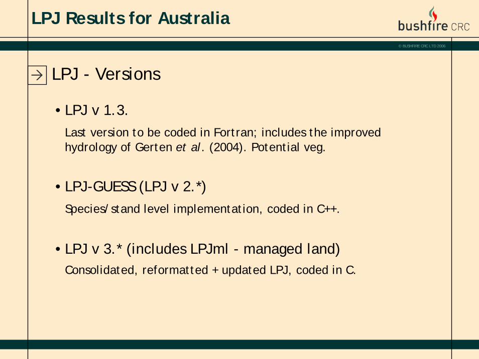
LPJ - Versions

•LPJ v 1.3.Last version to be coded in Fortran; includes the improved hydrology of Gerten et al. (2004). Potential veg.

•LPJ-GUESS (LPJ v 2.*)Species/stand level implementation, coded in C++.

•LPJ v 3.* (includes LPJml - managed land)Consolidated, reformatted + updated LPJ, coded in C.

LPJ Results for Australia


LPJ results – Average PFT Cover (1901-2000)

C3 perennial grass

Temp. needle evergreen

Trop. broad evergreen

C4 perennial grass

Temp. broad summergreen Trop. broad raingreen

Temp. broad evergreen


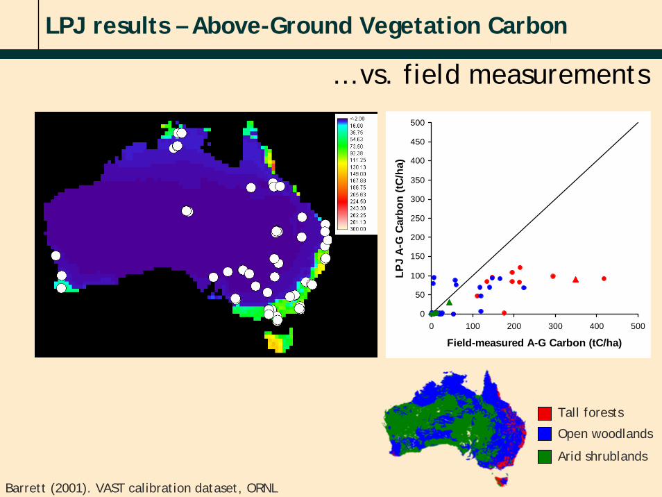
LPJ results – Above-Ground Vegetation Carbon

… vs. field measurements

0

50

100

150

200

250

300

350

400

450

500

0 100 200 300 400 500

Field-measured A-G Carbon (tC/ha)

LPJ

A-G

Car

bon

(tC/h

a)Tall forests

Open woodlands

Arid shrublands

Barrett (2001). VAST calibration dataset, ORNL


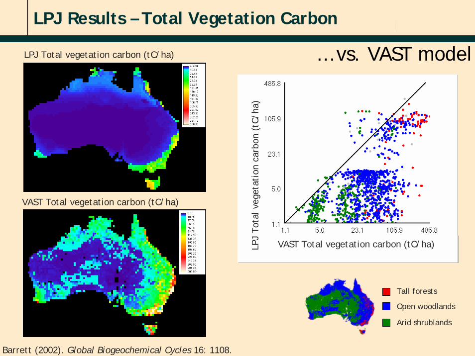
LPJ Results – Total Vegetation Carbon

… vs. VAST modelLPJ Total vegetation carbon (tC/ha)

VAST Total vegetation carbon (tC/ha)

LPJ

Tota

l veg

etat

ion

carb

on (

tC/h

a)VAST Total vegetation carbon (tC/ha)

Tall forests

Open woodlands

Arid shrublands

Barrett (2002). Global Biogeochemical Cycles 16: 1108.


LPJ Results – Fire, 1998-2000

Combined fire scar + fire hotspot observations (DOLA) LPJ

+=scar hotspot


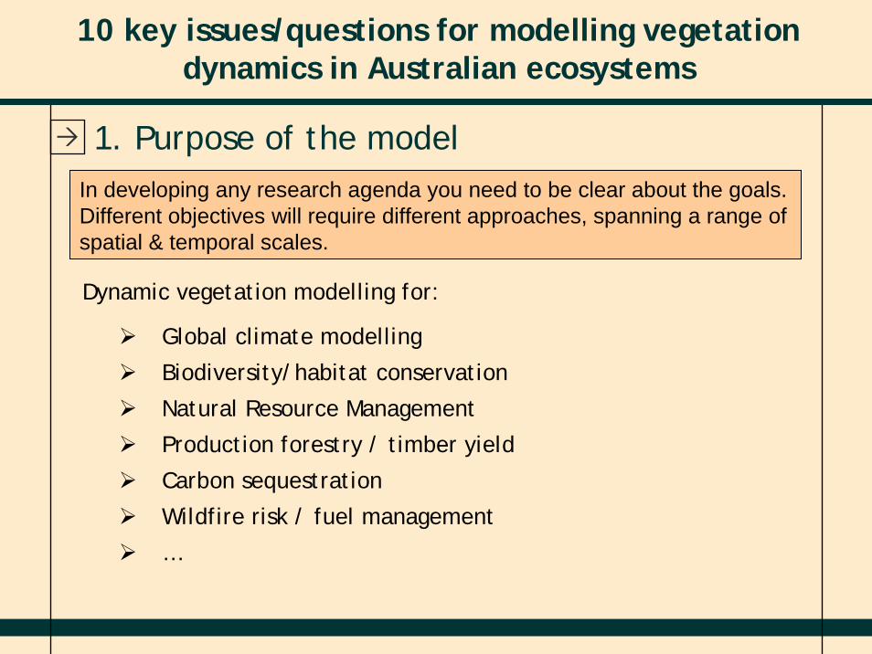
1. Purpose of the model

Global climate modelling

Biodiversity/habitat conservation

Natural Resource Management

Production forestry / timber yield

Carbon sequestration

Wildfire risk / fuel management

…

In developing any research agenda you need to be clear about the goals. Different objectives will require different approaches, spanning a range of spatial & temporal scales.

10 key issues/questions for modelling vegetation dynamics in Australian ecosystems

Dynamic vegetation modelling for:


DGVM’s operate at spatial scales that limit their utility at local/management scales (50km x 50km & above).

Can we adapt the DGVM framework to improve local-to-regional modelling of vegetation for environmental management? (finer-scaled PFT classifications? Finer spatial resolution?)

What local/regional processes need to be incorporated into current DGVM’s to improve their behaviour (watershed? firespread?)

What data do we need to calibrate and validate our models? (remote sensing technologies? Existing infrastructure – e.g. NCAS)

Scaling vegetation dynamics from local (Dynamic Landscape Vegetation Model), continental (Dynamic Continental Vegetation Model) to global (DGVM) is clearly a challenge. What data do we need for calibration + validation?

2. Scale of application & data requirements



3. Capturing variability / scaling.Most current approaches focus on ‘average’ descriptions of vegetation. E.g. ‘average’ or ‘typical’ parameter values are used to define generalised PFT’s. However, vegetation dynamics are inherently variable & nonlinear, and scaling correctly across time and space demands knowledge ofparameter variances and covariances, in addition to the averages.


How do we currently implement spatial and temporal scaling? (SEIB = brute force; ED = clever analytical approximations; LPJ = fudged through parameter tuning)

How do we communicate the importance of measuring variance and covariance (as well as average) as the key ingredient to scalingnonlinear processes?

Ruel, J.J & Ayres, M.P. 1999. Jensen’s inequality predicts effects of environmental variation. Trends in Ecology & Evolution 14: 361-366


4. Simplifying the Australian biota.Plant Functional Types (PFT’s) are the dominant paradigm for modelling large-scale dynamic vegetation patterns. Can we develop an optimal setof PFT’s for modelling Australian vegetation? Would such a set be globally applicable? Do we need PFT’s at all?


Current DGVM’s represent the distribution of vegetation in Australia poorly. Why?

Do we need to re-define/extend current PFT descriptions? Do we need to develop some new ones?

Do we need PFT’s at all?


Some vegetation processes are currently well known and described (e.g. photosynthesis), others remain poorly known and/or empirical (e.g. photosynthate allocation, plant competition, succession).

Some important processes have not received the attention they deserve: genetic variability and the capacity of vegetation to evolve; dispersal/migration rates.

Some Australian-specific vegetation dynamics/processes demand attention (woodland thickening, fate of Alpine biota, …)

5. Level of process description required.Empirical relationships based on current/past conditions may not remain valid under a changed climate. Predictive modelling therefore requires a certain level of process description.



6a. Spatially contagious processes – large scale.Most global/continental vegetation models do not allow energy and matter to pass from gridcell-to-gridcell, and assume that such dynamics are mostly within-gridcell phenomenon. In Australia there may be exceptions to this rule (e.g. continental-scale rainfall re-distribution, ‘megafire’).

2006/07

2003

Recent major bushfires

200km

Continental water courses



6b. Spatially contagious processes – fine scale.At the landscape-scale horizontal fluxes (e.g. above and below-ground water movement), fire spread, and the redistribution of organisms (e.g. dispersal, invasion) are important processes. How do we capture these?


Kioloa landscape, NSW Angophora costata stand, Queensland


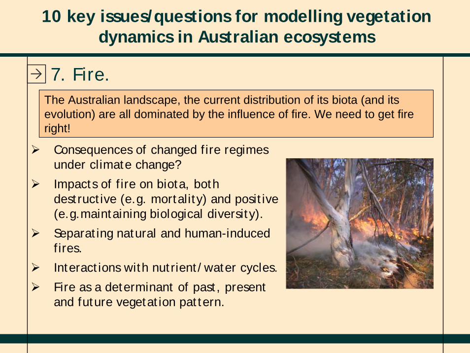
7. Fire.The Australian landscape, the current distribution of its biota (and its evolution) are all dominated by the influence of fire. We need to get fire right!


Consequences of changed fire regimes under climate change?

Impacts of fire on biota, both destructive (e.g. mortality) and positive (e.g.maintaining biological diversity).

Separating natural and human-induced fires.

Interactions with nutrient/water cycles.

Fire as a determinant of past, present and future vegetation pattern.


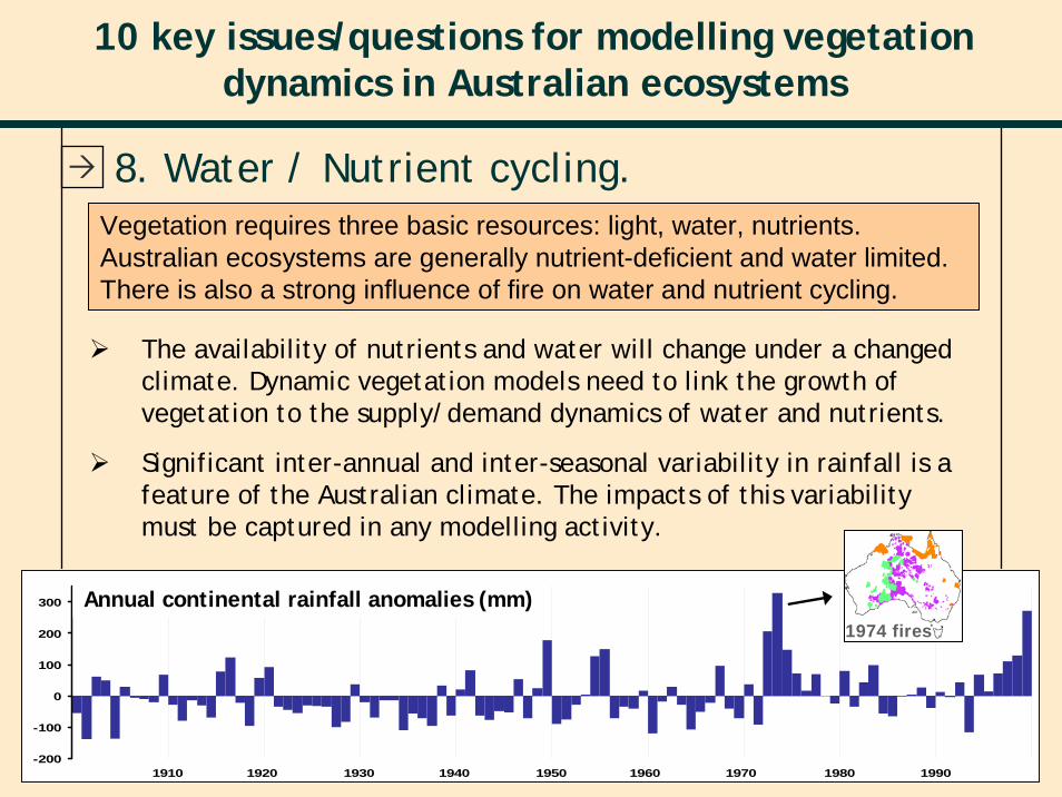
8. Water / Nutrient cycling.Vegetation requires three basic resources: light, water, nutrients. Australian ecosystems are generally nutrient-deficient and water limited. There is also a strong influence of fire on water and nutrient cycling.


The availability of nutrients and water will change under a changed climate. Dynamic vegetation models need to link the growth of vegetation to the supply/demand dynamics of water and nutrients.

Significant inter-annual and inter-seasonal variability in rainfall is a feature of the Australian climate. The impacts of this variability must be captured in any modelling activity.

-200

-100

0

100

200

300

1910 1920 1930 1940 1950 1960 1970 1980 1990

Annual continental rainfall anomalies (mm)1974 fires


9. Herbivory.Herbivores consume vegetation! 10%-20%(?) of global NPP is consumed by native, domestic, feral and insect herbivores.


Cattle + sheep; DSE/ha Horse + goat + camel + donkey; DSE/ha

DSE = Dry Sheep Equivalent


10. Land management.Most DGVM’s start with the assumption of ‘natural’ or ‘potential’vegetation. For real-life application the influence of land management must also be included


Descriptive (e.g. using historical records) vs. predictive (e.g. human behaviour and land-use models)

Requires an understanding of the impacts on water/nutrient cycles, carbon balance…

Agricultural, rangeland management, native forest harvesting, plantation forestry

Above-ground tree carbon

0

5

10

15

20

25

30

35

40

45

50

40 50 60 70 80 90 100

Time(years)

tC/h

a

Cotton plantation, NSW

Model-predicted + observed recovery of Poplar Box following chaining



• What are the objectives?

• Scale of application & data requirements

• Capturing variability / scaling

• Level of process description required?

• Simplifying the Australian biota

• Spatially contagious processes

• Fire

• Water / Nutrient cycling

• Herbivory

• Land management

A modelling perspective for framing thoughts on vegetation ... · LPJ results – Average PFT Cover...

Documents

Transcript of A modelling perspective for framing thoughts on vegetation ... · LPJ results – Average PFT Cover...