A MODEL FOR MATRIX ACIDIZING OF LONG HORIZONTAL …

A MODEL FOR MATRIX ACIDIZING OF LONG HORIZONTAL WELL IN

CARBONATE RESERVOIRS

A Thesis

by

VARUN MISHRA

Submitted to the Office of Graduate Studies of Texas A&M University

in partial fulfillment of the requirements for the degree of

MASTER OF SCIENCE

August 2007

Major Subject: Petroleum Engineering

A MODEL FOR MATRIX ACIDIZING OF LONG HORIZONTAL WELL IN

CARBONATE RESERVOIRS

A Thesis

by

VARUN MISHRA

Submitted to the Office of Graduate Studies of

Texas A&M University in partial fulfillment of the requirements for the degree of

MASTER OF SCIENCE

Approved by:

Chair of Committee, Ding Zhu Committee Members, A. Daniel Hill

P. Daripa Head of Department, Stephen A. Holditch

August 2007

Major Subject: Petroleum Engineering

iii

ABSTRACT

A Model for Matrix Acidizing of Long Horizontal Well in Carbonate Reservoirs.

(August 2007)

Varun Mishra, B.Tech., Indian School of Mines Chair of Advisory Committee: Dr. Ding Zhu

Horizontal wells are drilled to achieve improved reservoir coverage, high production

rates, and to overcome water coning problems, etc. Many of these wells often produce at

rates much below the expected production rates. Low productivity of horizontal wells is

attributed to various factors such as drilling induced formation damage, high completion

skins, and variable formation properties along the length of the wellbore as in the case of

heterogeneous carbonate reservoirs. Matrix acidizing is used to overcome the formation

damage by injecting the acid into the carbonate rock to improve well performance.

Designing the matrix acidizing treatments for horizontal wells is a challenging task

because of the complex process. The estimation of acid distribution along wellbore is

required to analyze that the zones needing stimulation are receiving enough acid. It is

even more important in cases where the reservoir properties are varying along the length

of the wellbore.

A model is developed in this study to simulate the placement of injected acid in a long

horizontal well and to predict the subsequent effect of the acid in creating wormholes,

overcoming damage effects, and stimulating productivity. The model tracks the interface

between the acid and the completion fluid in the wellbore, models transient flow in the

reservoir during acid injection, considers frictional effects in the tubulars, and predicts

the depth of penetration of acid as a function of the acid volume and injection rate at all

locations along the completion. A computer program is developed implementing the

developed model. The program is used to simulate hypothetical examples of acid

placement in a long horizontal section. A real field example of using the model to

history match actual treatment data from a North Sea chalk well is demonstrated. The

model will help to optimize acid stimulation in horizontal wells.

iv

DEDICATION

To my parents and friends, the source of my inspiration.

v

ACKNOWLEDGMENTS

I would like to thank to my advisors, Dr. Ding Zhu and Dr. A. Daniel Hill, who guided

me throughout the course of this research with extraordinary kindness and patience.

I would also like to thank the sponsors of the Middle East Carbonate Stimulation joint

industry project at Texas A&M University for support of this work. Finally, thanks to Dr.

Prabir Daripa, for his help and support for being a member of my committee.

vi

TABLE OF CONTENTS

Page

ABSTRACT ................................................................................................................iii

DEDICATION.............................................................................................................iv

ACKNOWLEDGMENTS.............................................................................................v

TABLE OF CONTENTS.............................................................................................vi

LIST OF FIGURES ................................................................................................... viii

LIST OF TABLES........................................................................................................x

CHAPTER

I INTRODUCTION.......................................................................................1

1.1 Background......................................................................................1 1.2 Literature review..............................................................................2 1.3 Objective and approach....................................................................4

II MATRIX ACIDIZING MODEL DEVELOPMENT....................................6

2.1 Wellbore flow model .......................................................................7 2.1.1 Wellbore material balance ...................................................7 2.1.2 Wellbore pressure drop........................................................8

2.2 Reservoir flow model.......................................................................9 2.3 Model for tracking fluid interfaces ..................................................10 2.4 Wormhole model ............................................................................11

2.4.1 Volumetric wormhole model .............................................12 2.4.2 Buijse’s semiempirical wormhole model ...........................12

2.5 Skin and well completion model .....................................................15 2.5.1 Formation damage skin......................................................16 2.5.2 Cased and perforated completions .....................................18

2.5.3 Slotted liner completions ...................................................24 2.5.4 Partial penetration skin model............................................28 2.5.5 Solution of matrix acidizing model ....................................31

III MATRIX ACIDIZING SIMULATOR .......................................................33

3.1 Matrix acidizing simulator ..............................................................33 3.2 Simulator data files .........................................................................34

3.2.1 Input data file ...................................................................34 3.2.2 Output data files ...............................................................35

vii

CHAPTER Page

IV RESULTS..................................................................................................36

4.1 Hypothetical examples ....................................................................36 4.1.1 Horizontal well with openhole completion........................36 4.1.2 Horizontal well with cased-perforated completion ............42 4.1.3 Horizontal well with slotted liner completion....................46 4.1.4 Heterogeneity effect in horizontal well acidizing ..............49

4.2 Field study ......................................................................................53

V CONCLUSIONS........................................................................................59

5.1 Conclusions ....................................................................................59

REFERENCES ...................................................................................................60

NOMENCLATURE............................................................................................62

APPENDIX A MATRIX ACIDIZING SIMULATOR ......................................67

APPENDIX B MATRIX ACIDIZING SIMULATOR INPUT DATA FILE......76

VITA ..................................................................................................................79

viii

LIST OF FIGURES

FIGURE Page

2.1 Schematic of a section of wellbore during an acidizing process ........................7

2.2 Interface movement inside the wellbore.......................................................... 11

2.3 Pore volume to breakthrough as a function of injection rate............................ 14

2.4 Openhole horizontal well with formation damage around wellbore................. 17

2.5 Growth of wormhole from the tip of the perforation ....................................... 18

2.6 Perforation skin components .......................................................................... 19

2.7 Perforated well with deep penetration of damage............................................ 22

2.8 Perforated well with shallow penetration of damage ....................................... 23

2.9 Geometric variables for slotted liner skin calculation...................................... 24

2.10 Flow geometries around a slotted liner ........................................................... 25

2.11 A section of partially completed vertical wellbore .......................................... 28

2.12 Horizontal well partially open to the reservoir ................................................ 29

2.13 Ellipsoidal flow geometry............................................................................... 30

4.1 Acid coverage over the entire length of wellbore ............................................ 39

4.2 Wormhole length distributions at different times ............................................ 39

4.3 Acid placement profiles for 200 and 500 bbls of acid ..................................... 40

4.4 Acid placement profiles for different values of PVbt........................................ 40

4.5 Pressure responses during acid injection ......................................................... 41

4.6 PVbt versus Vi during simulation using Buijse Model with PVbt-opt=1.5 ........... 41

4.7 Comparison of wormhole distributions from volumetric and Buijse’s models. 42

4.8 Distribution of perforation length along the wellbore...................................... 44

4.9 Evolution of skin with time during acid injection............................................ 44

4.10 Acid coverage in cased-perforated completion case ........................................ 45

4.11 Distribution of wormholes in cased-perforated completion case...................... 45

4.12 Comparison of acid coverage in uniform and non-uniform perforation length

distribution..................................................................................................... 46

4.13 Distribution of wormhole length in slotted liner completion ........................... 48

ix

FIGURE Page

4.14 Distribution of skin in slotted liner completion ............................................... 48

4.15 Distribution of initial damage along the length of wellbore............................. 50

4.16 Distribution of permeability along the length of wellbore ............................... 50

4.17 Acid coverage along the length of wellbore .................................................... 51

4.18 Injectivity index during the acid injection....................................................... 52

4.19 Local skin factors along the wellbore at the end of simulation ........................ 52

4.20 Selective stimulation for each perforated zone using straddle packers and

perforated coiled tubing.................................................................................. 53

4.21 Pressure response of downhole gauges ........................................................... 54

4.22 Rate schedule for North Sea field well acid treatment ..................................... 54

4.23 History match of treatment pressure ............................................................... 56

4.24 Acid placement for North Sea field well ......................................................... 57

A.1 A schematic of segmented wellbore................................................................ 70

A.2 A flow chart for matrix acidizing simulator .................................................... 73

x

LIST OF TABLES

TABLE Page 2.1 Correlation constant, am.............................................................................................................................................21

2.2 Correlation constants, bm and cm ........................................................................................................................21

2.3 Correlation constants, dm em, fm and gm........................................................................................................21

3.1 Matrix acidizing simulator data files....................................................................34

4.1 Data for acid injection into horizontal well with openhole completion.................37

4.2 Data for acid injection into horizontal well with cased-perforated completion .....43

4.3 Data for acid injection into a horizontal well with slotted liner completion ..........47

4.4 Data for acid injection into a horizontal well with thief zones..............................49

4.5 Input data for North Sea field well.......................................................................55

1

CHAPTER I

INTRODUCTION

1.1 Background

Starting in the 1980s, horizontal wells began capturing an ever-increasing share of

hydrocarbon production. They proved to be excellent producers for thin (h<50 ft)

reservoirs or for thicker reservoirs with good vertical permeability, kV.

Horizontal wells are drilled to achieve improved reservoir coverage, high production

rates, and to overcome water coning problems etc. Many of these wells often produce at

a rate below the expected production rates. Low productivity of horizontal wells is

attributed to various factors such as drilling induced formation damage, high completion

skins, and variable formation properties along the length of the wellbore as in the case of

heterogeneous carbonate reservoirs.

Positive skin effects are created by “mechanical” causes such as partial completion, by

altering the relative permeability of original fluid, by turbulence, and by damage to the

original permeability. Formation damage in horizontal wells is unavoidable due to

longer exposure time of wellbore to the drilling and completion fluid. The fine particles

contained in drilling fluid migrate inside the formation rock and plug the pore spaces

which results in reduction of formation permeability1.

Investigations in the past have shown that positive skins are detrimental to the

performance of horizontal wells. Various completion techniques are also adopted for

horizontal wells such as openhole completions, cased perforated completions, and

slotted liner completions. These completions may also contribute to the positive skin

factors resulting in much higher skin values than damage skin alone.-

Matrix acidizing is a techniques to stimulate the well by removing near wellbore damage.

In sandstone reservoirs, matrix acidizing is often considered for many people as risky to

This thesis follows the style of SPE Production and Operations.

2

undertake due primarily to heterogeneous nature of formation minerals and an

appreciable degree of unpredictability of their response to acid formulations2; however,

in carbonate reservoirs it is a relatively simple stimulation technique that has became one

of the most cost-effective method to improve significantly the well productivity and

hence the hydrocarbons recovery. The success rate of the treatments in carbonate

reservoirs is 30%-50%.

During matrix acidizing treatments the acid is injected at pressures below the fracture

pressure to avoid fractures being created during the treatments. The acid reacts within a

few inches from wellbore in sandstones and a few feet in carbonates1. In carbonate

formations matrix acidizing is used as a tool to overcome the formation damage by

injecting the acid into the carbonate rock which results in formation of wormholes.

Acid stimulation is a cost effective method to enhance the productivity of horizontal

wells in carbonate reservoirs. Acid can be injected by bullheading down the production

tubing, through coiled tubing, or into intervals by isolating packers, or injection from

acid jetting tools. Effective stimulation requires that sufficient acid volume be placed in

all desired zones.

1.2 Literature review

Designing the matrix acidizing treatments for horizontal wells is a challenging task

because of the complex processes involved. The acid distribution along the wellbore is

hard to predict and it becomes more difficult in case of varying reservoir properties

along the wellbore.

Jones and Davies3 made an attempt to quantify the acid placement in horizontal wells.

According to them the key to the treatment success is maximizing the acid coverage over

the length of the wellbore. The model presented was for barefoot completions in

sandstone formations and the simulator used a pseudo-steady state reservoir model. They

concluded that variation in reservoir properties along the treatment interval significantly

impacts the acid placement over the wellbore length. The need to include wellbore

phenomena was also emphasized in their work.

3

Buijse and Glasbergen4 used a placement simulator to predict the zonal coverage of

stimulation fluids in long vertical wellbore. The fluid placement simulator was based on

the model described by Davies and Jones. The model assumes a piston type

displacement between various fluids in the wellbore. They used different diversion

methods in simulating the stimulation treatments in long intervals. Based on the

simulation results it was concluded that the fluid distribution in heterogeneous

formations such as carbonate reservoirs can only be understood to its full extent by using

a numerical simulator. To evaluate a past design or to optimize a future acidizing

treatment a fluid placement simulator is essential. Their conclusion also holds true for

long horizontal wells placed in carbonate reservoirs. Carbonate reservoirs are

heterogeneous in nature and horizontal wells drilled in carbonate reservoirs most likely

have non-uniform formation properties along the wellbore length. During acid

treatments of these wells heterogeneity causes difficulty in predicting the distribution of

acid along the entire wellbore length. So a fluid placement simulator is necessary to

understand the resulting fluid distribution thus optimizing the future treatments.

Eckerfield et al.5 concluded in their work that movement of interfaces formed between

acid and completion fluids is significantly affected by uneven reservoir flow distribution,

which ultimately leads to nonuniform volume of acid injected into the formation.

Wellbore hydraulics was found to have much less impact because of the small wellbore

volume relative to the volume of acid injected.

Gdanski6 described recent advances in carbonate stimulation stating that zonal coverage

of long carbonate sections remains a challenge and most of the acidizing treatments are

designed on the basis of past experience.

A study was conducted by Bazin et al.7 to optimize the strategy for matrix treatment of

horizontal drains in carbonate reservoirs. It was concluded that there should always be a

well defined strategy for acidizing treatments of horizontal wells depending on the

reservoir characteristics and no “rule of thumb” should be used else it may results in

poor stimulation.

4

The acid placement techniques also play an important role in effective stimulation of the

horizontal wells. Mitchell et al.8 compared two acid placement techniques i.e.

bullheading and coiled tubing injection used in offshore fields of Java Sea. The authors

concluded in their work that coiled tubing stimulation provides a greater increase in

productivity index which sustains for longer period of time. It was found that the coiled

tubing enable stimulation fluids to be placed where they are needed. The additional cost

of using the coiled tubing can be offset by the incremental production but offshore

operating conditions limit the use of coiled tubing. In such cases injection through

bullheading was found as an inexpensive way to stimulate the wells.

1.3 Objective and approach

The presented research project aims to develop an acid stimulation model to study the

acid distribution and evolution of skin during acidizing treatments in the horizontal wells

in carbonate reservoirs. This model considers the frictional pressure drop along the

wellbore. It tracks interfaces between various injected fluids and models the transient

flow response of the reservoir. The model couples a wellbore flow model, an interface

tracking model, a wormhole model, a skin evolution model, and a transient reservoir

inflow model. The model predicts the bottomhole pressure response during an acid

treatment, the distribution of acid along the treated section, and the resulting skin factor

during stimulation. This model is capable of handling the variable formation properties

along the wellbore such as porosity, permeability, etc.

The formulation of the various model equations is presented in Chapter II. The model

couples several processes together. Each process is described separately in this chapter.

A method to solve the model equations is also presented in this chapter.

A computer program is developed incorporating the new model which can be used to

design and evaluate the acidizing treatments in long horizontal wells. Using the

developed computer program an analysis of the evolution of skin and acid coverage will

be performed for past as well as future treatments. In Chapter III, the program flow chart

and information about input and output data files are presented.

5

In Chapter IV, results of hypothetical cases and actual field studies are presented. One

hypothetical case is presented assuming uniform distribution of reservoir properties

along the wellbore. The effect of variable formation properties is also studied using the

developed program. It was found that their effect is significant on the acid distribution

along the wellbore.

A field case is presented in which a history match of observed pressure data and

simulated pressure data was done by varying parameters which influence the treatment.

The analysis of acid treatments in small wellbore section is done using the developed

model. The impact of partial penetration skin on acid treatment response is investigated.

The lessons learned by evaluating the past treatments might pave a way to optimize our

future treatments to achieve higher productivities from the horizontal wells.

6

CHAPTER II

MATRIX ACIDIZING MODEL DEVELOPMENT

In this chapter, an acidizing model for horizontal well is presented. In a typical matrix

acidizing process the acid is injected into the formation through production tubing,

coiled tubing, or drill pipe. The acid displaces the wellbore fluid, forming interfaces

between different fluids. The acid flows into the formation and creates wormholes in the

reservoir rock, increasing the injectivity of the contacted portions of the formation. The

effect of acid on the formation injectivity at any location along the well is accounted for

with a local skin factor that is changing in response to the acid injected at that point.

Local injectivity is simultaneously affected by the transient nature of the process as

injection of any fluid causes a pressure build up in the porous medium. The transient

pressure build up due to the injection and the acid stimulation that is increasing

injectivity are competing effects that must both be considered to properly predict acid

placement.

To simulate the acidizing process above, all of the processes are studied separately.

These include a wellbore model which handles the pressure drop and material balance in

the wellbore; an interface tracking model to predict the movement of interfaces between

different fluids in the wellbore; a transient reservoir flow model; a skin factor model

accounting for partial penetration and well completion effects; and, an acid stimulation

model that predicts wormhole growth and the effects these have on local injectivity.

Each model is discussed in this chapter separately.

The coupled model allows for an arbitrary distribution of perforations along the

completion, initial damage, reservoir permeability, and a user-specified acid treatment

schedule. The model predicts the acid coverage and wormhole penetration as functions

of position along the wellbore and injection time. A solution scheme is presented to

simulate the bottomhole pressure response during the treatment. This response can be

matched with the actual pressure response during the treatment.

7

2.1 Wellbore flow model

The wellbore flow model is developed based on wellbore material balance and wellbore

pressure drop calculations. The fluids injected during the acid injection process are

mostly incompressible so single phase incompressible flow in the wellbore is assumed to

develop these equations.

2.1.1 Wellbore material balance

Figure 2.1 shows a schematic of a horizontal wellbore during an acid injection process.

Single phase (liquid) flow through a reservoir injected by a fully penetrating horizontal

well is considered. It is also assumed that all of the reservoir flow is perpendicular to the

wellbore. pw is wellbore pressure at any point in the wellbore, qw is the flow rate in the

wellbore, and qR is specific reservoir outflow i.e. per unit length. Since the flow rate

changes along the wellbore is caused by the fluid flowing into the reservoir, by material

balance, we have,

Rw qx

q−=

∂∂

(2.1)

Equation 2.1 states that the specific reservoir outflow, qR (bbl/ft) should be equal to the

decrease in wellbore flow rate per unit length, qw (bbl).

Figure 2.1 Schematic of a section of wellbore during an acidizing process

qR(x,t)

qw(x,t)pw(x,t)x

r

qR(x,t)

qw(x,t)pw(x,t)x

r

8

2.1.2 Wellbore pressure drop

If steady state flow exists in a horizontal pipe and fluid has a constant density, then

friction pressure drop is obtained from the Fanning equation1,

(2.2)

In the differential form the above equation can be written as,

dguf

xp

c

fw22 ρ

−=∂

∂ (2.3)

In the above equation ff is defined as the Fanning friction factor, and u is defined as the

fluid velocity.

Aq

u w= (2.4)

Equation 2.4 relates the fluid velocity with the flow rate; where A is the cross-section

area of the pipe and qw is the fluid flow rate in the pipe. Eq. 2.3 is rearranged for the oil

field units as;

5

2525.1

d

qf

xp w

fw ρ

−=∂

∂ (2.5)

Where pw is in psi, x is in ft, ρ is in lbm/ft3, d is in inches, and qw is in bpm.

Equation 2.5 provides the equation for pressure drop in a horizontal wellbore during the

acid injection process. This equation will be coupled with the other system equations to

setup the matrix acidizing model.

The Fanning Friction factor depends on the Reynolds number, NRE, and pipe roughness,

ε. Fluid flow is characterized as laminar or turbulent, depending on the value of the

Reynolds number, NRE, defined for a circular pipe as

µρduN =Re (2.6)

dgLuf

Pc

pipefF

22 ρ=∆

9

Consistent units must be used in the evaluation of the Reynolds number so that NRe is

dimensionless. Laminar flow exists within the pipe when Reynolds number is less than

2000. For turbulent flow, Reynolds number is greater than 4000. The flow is called

transitional, if Reynolds number lies between 2000 and 4000.

The Fanning friction factor is most commonly obtained from the Moody friction factor

chart. But for computational purposes the following equations are used to determine the

friction factor. In laminar flow, the friction factor is inversely related to the Reynolds

number as;

Re

16N

f f = (2.7)

For turbulent flow, an explicit equation for the friction factor is the Chen equation1;

+−−=

8981.0

Re

1098.1

Re10

149.78257.2

0452.57065.3

log41NNf f

εε (2.8)

Parameter obtained from the pressure drop equation, i.e. pw or qw, from the wellbore

model will be used in the reservoir flow model.

2.2 Reservoir flow model

During the acidizing process, the wellbore rate and the reservoir inflow at any location

are changing with time so transient effects are occurring in the reservoir. With the

superposition principle the outflow estimation to include the transient effects during acid

injection process can be estimated as9;

( ) [ ] nnDjnDn

jjwR sqttpqppkl +−∆=−− −

=∑ )(2

11µ

π (2.9)

Where:

1−−=∆ jjj qqq (2.10)

10

2

610395.4

wtD

rc

kttφµ

−×= (2.11)

)80907.0(ln21 +≈ DD tp (2.12)

Equation 2.9 provides the wellbore pressure (pw) at nth time step when the reservoir

inflow rate, q, is varying with time. pR is defined as initial reservoir pressure when there

was no flow from the wellbore to the reservoir. The parameter s in the Eq. 2.9 represents

the local skin factor and it changes continuously with acid injection. Reservoir

permeability, porosity, compressibility and injected fluid viscosity are defined as k, Φ, ct,

and µ, respectively. rw is wellbore radius. All of the variables used in the equations are in

oil field units as defined in the appendix.

Once the reservoir outflow and transient pressure response is obtained, it is required to

calculate the volume of specific fluid injected into the formation. As during injection,

multiple interfaces may exist, an interface tracking model is used to calculate the

position of an interface. Once locations of the interfaces are obtained the volume

injected behind the fronts are to be calculated.

2.3 Model for tracking fluid interfaces

A model to track the interfaces created between various injected fluids was presented by

Eckerfield et al.5 This acid placement model will use a discretized solution approach

which is integrated with the reservoir flow, wormhole, and skin models. Fig. 2.2 depicts

a part of the wellbore where the interface created between injected acid and wellbore

fluid is traveling to the right. The velocity of an interface located at xint is simply,

int

int

xx

wA

qdt

dx

== (2.13)

11

Injected acid

Xint|t=t Xint|t=t+∆t

Aqw

∆t

Figure 2.2 Interface movement inside the wellbore

In discrete form the location of interface at time (t+∆t) can be written as

tA

qxxxx

wttttt ∆+=

==∆+=

intintint (2.14)

where A is the cross-sectional area of flow in the pipe. Eq. 2.14 is solved by discretizing

the wellbore into small segments and assuming constant qw over each segment.

Once the interfaces and outflows in the wellbore parts are estimated it is necessary to get

the growth of wormhole during that injection time. A wormhole model is applied with

injection volume or rate as input to get the wormhole growth. Length of wormhole is

calculated by integrating growth in every small time step.

2.4 Wormhole model

When the acid (HCl) is injected into carbonate rocks, due to very high surface reaction

rates, mass transfer limits the overall reaction rate, leading to highly nonuniform

dissolution pattern, and few large channels are formed known as wormholes. Wormholes

bypass the damaged near wellbore region and improve the flow conditions. Creation of

wormholes and optimization of the wormhole length are main goals in acid treatment

design. It is important to gain an understanding of parameters that affect the wormhole

growth. Structure of these wormholes depends on many factors such as flow geometry,

injection rate, reaction kinetics, and mass transfer rate.

12

Fredd and Miller10 presented an excellent review of the different models that have been

presented in the past. The authors work was focused on validating the wormhole models

with the laboratory data from linear flow experiments. Two models of the wormholing

process will be implemented in this work.

2.4.1 Volumetric wormhole model

The volumetric model1, 11 is based on the assumption that a constant fraction of the rock

volume is dissolved in the region penetrated by wormholes. For radial flow, the

volumetric model is

btwwh PV

lVrrπφ

/2 += (2.15)

where rwh is distance of wormhole tip from the wellbore center, V/l is the volume of acid

injected per unit length of formation. When only a few wormholes are formed, a small

fraction of the rock is dissolved; more branched wormhole structures dissolve larger

fractions of the matrix. The key parameter in this model is PVbt, the number of pore

volumes of acid needed to propagate a wormhole through a certain distance. The PVbt

can vary in a large range, depending mainly on the rock mineralogy.

If the PVbt is obtained from a radial core flood, it should predict wormhole propagation

in a well treatment where the flow is radial, at least for wormhole propagation to the

same distance as that tested in the core flood. If a linear core flood is used to measure

PVbt, the wormhole propagation in radial flow will probably be somewhat overestimated.

2.4.2 Buijse’s semiempirical wormhole model

An improved empirical model of the wormholing process is presented by Buijse and

Glasbergen12. The authors adopted an alternative approach and described the wormhole

growth by a simple model. In this model the growth rate of the wormhole front is

modeled as a function of acid injection rate which is in fact related to acid velocity in the

pores. The effect of acid velocity is more significant in case of perforated completions.

This model is semiempirical as the effect of parameters such as temperature, acid

13

concentration; permeability and mineralogy are not modeled explicitly. The effect of

these parameters is included in the model in two constants, Weff and WB. The value of

these constants can be calculated from the results of a core flow experiment in the

laboratory or by fitting the model to field results.

According to this model, in radial geometry, the wormhole growth rate depends on the

injection rate and also on the position of the wormhole front in the formation. The

interstitial fluid velocity is defined as,

φπrlQVi 2

= (2.16)

where r is the distance of the wormhole tip from the center of the wellbore. Eq. 2.16

explains that how the interstitial fluid velocity and the wormhole length are inversely

related. The wormhole velocity is can be also calculated as,

BVWV ieffwh .. 3/2= (2.17)

where parameter Weff ,WB , and B can be calculated by using Eqs. 2.18, 2.19, and 2.20 as,

( )( )22.exp1 iB VWB −−= (2.18)

optbt

optiPVV

Weff−

−=3/1

(2.19)

24

optiB

VW

−= (2.20)

Ideally the constants Weff and WB are calculated from the results of radial core flow tests.

The radial core flow tests are difficult and expensive to perform and sometimes there are

no data available. In that case these constants can be determined using the data of linear

core flow tests in Eqs. 2.19 and 2.20. The optimum values of fluid velocity, Vi-opt, and

break through pore volume, PVbt-opt, can be obtained from the liner core flow tests.

14

Once the wormhole velocity is obtained, the growth of the wormhole can be obtained by

discretizing the time domain as the wormhole velocity depends on the interstitial fluid

velocity, which in turn depends on the distance of wormhole tip from the center. In this

model, the wormhole propagation rate varies with the acid flux in a manner based on the

commonly observed “optimal flux” behavior. The optimal acid flux and the optimal PVbt

are based on laboratory tests.

The authors gathered the data for core flow tests results from in-house experiments and

from literature. A log-log plot of this data is shown in Fig. 2.3 where the pore volumes to

breakthrough are plotted as a function of injection rate. The curves are fitted to the

measured data points using the equation below,

BW

VVV

PVeff

i

wh

ibt

3/1== (2.21)

Figure 2.3 Pore volume to breakthrough as a function of injection rate12

Equation 2.21 explains that with changing interstitial fluid velocity, i.e. Vi, the pore

volumes for breakthrough changes and it does not remain constant during the injection

as in volumetric wormhole model. It can be seen from the Fig. 2.3 that on this log-log

plot, there exists an optimum value of PVbt and Vi , which are termed as PVbt-opt and

15

Vi-opt. During the acid injection treatments, if the interstitial fluid velocity falls below the

optimum i.e. Vi-opt , the PVbt increases with the decreasing Vi and the face dissolution of

carbonate rock occurs. If the acid is injected at the rate so that interstitial fluid velocity

remains above the optimum, the PVbt decreases with the decreasing Vi. So at high

interstitial fluid velocities, B approaches to 1 and Eq. 2.21 holds true,

3/2

3/1

iwh

ibt

VV

VPV

∝

∝ (2.22)

During the acid injection in field conditions, the Buijse’s model recommends the acid

injection rate to be maintained above the optimum injection rate but staying below the

fracturing pressure. Both of the models, the volumetric and the Buijse’s model of

wormhole propagation are to be implemented in the acidizing simulator. If the PVbt input

to the volumetric model is close to the average value of PVbt (as it changes throughout

the injection) determined by the Buijse’s model at the acid flux occurring in the

simulated acid treatment, the results from these two models should be similar.

The wormhole model provides the length of wormhole as an input to the skin model,

which then calculates the skin factor. Skin factors are updated at every time step.

2.5 Skin and well completion model

The horizontal wells drilled in carbonate reservoirs can be completed with several

completion techniques. The common completion types are openhole completions, cased

and perforated completions and slotted liner completions. Positive skin factors are found

in openhole completions mostly due to formation damage. The other two completion

techniques might introduce positive completions skin factors along with the formation

damage skin.

The changing injectivity during acid injection is accounted for with a local skin factor,

s(x), which includes the effects of the completion, possible formation damage, and

stimulation with a positive value for completion, and a negative value for stimulation.

The effects of the completion, formation damage, and stimulation are all coupled.

16

During the matrix acidization process the wormholes are created and propagate into the

formation. The propagation of wormholes into the formation lowers the skin and

enhances the productivity of the well. The evolution of skin factors for each type of

completions are discussed in separate sections.

In addition, injectivity of individual zones along a long horizontal well are affected by a

partial penetration effect which can be treated as a skin effect. This partial penetration

effect is also described in later section.

2.5.1 Formation damage skin

Formation damage occurs due to the reduction in original permeability of the rock. The

original permeability can be altered due to fines migration from drilling and completion

fluid, or relative permeability alteration etc. In openhole completions, the damage skin

can cause sufficient pressure drop to reduce the production rate. In openhole completions

the wellbore have direct contact with the formation and whole cylindrical surface area of

wellbore is open to flow.

Openhole completions are the simplest and the cheapest. Their use is restricted to

reservoirs formed of competent rock that is sufficiently strong to withstand collapsing

stresses. Openhole completions provide the maximum flexibility for future well

modification. For example, it is possible, at a later stage, to insert a liner with external

casing packers or even to convert an open hole well to a fully cemented completion.

Figure 2.4 shows an openhole completion of a horizontal well with formation damage in

the near wellbore region. rd is defined as the damaged radius beyond the wellbore and

rwh is defined as the length of the wormholes. Ideally these two parameters vary with the

length and may have a nonuniform distribution along the length of the wellbore.

17

Figure 2.4 Openhole horizontal well with formation damage around wellbore

Under the assumption that the pressure drop in the wormhole is small, these wormholes

can be considered as infinite conductivity channels. The local skin factor at any general

point x along the wellbore can be achieved by applying the Hawkins formula for skin at

that point.1

For rwh<rd:

−

=

w

d

wh

d

d rxr

xrxr

xkkxs

)(ln

)()(

ln)(

)( (2.23)

And for rwh>rd:

−=

w

whr

xrxs

)(ln)( (2.24)

where rwh is radius of region penetrated by wormholes at that particular point, which is

to be calculated from the wormhole model.

It is evident from the above equations that as the wormholes grow longer the skin factor

decreases. The skin factor needs to be updated at each time step after calculating the

wormhole length at the end of time step.

L

d rwhr

Wormholes

Damaged ZoneUndamaged Zone

w r

L

d rwhr

Wormholes

Damaged ZoneUndamaged Zone

w r

18

2.5.2 Cased and perforated completions

Cased and perforated completions are also a commonly used method for horizontal well

completion. Perforation is the communication tunnel extending beyond casings or liners

into the reservoir formation, through which oil or gas is produced. In most cases, a high

penetration is desirable to create effective flow communication to the part of the

formation that has not been damaged by the drilling or completion processes.

perforationwormhole

casing

wellbore

damaged zone formation

Figure 2.5 Growth of wormhole from the tip of the perforation

For a cased, perforated completion, the perforation skin factor model of Furui et al.13 is

used. The model assumes that wormholes propagating from the tips of perforations can

be considered as extensions of the effective lengths of the perforations as in Fig. 2.5.

On the basis of above assumption the effective length of perforation at any time step can

be written by Eq. 2.25,

whpeffp rll +=, (2.25)

where lp is perforation length which remains constant over time, lp,eff is effective

perforation length at certain time, and rwh is length of wormhole at that time.

19

Figure 2.6 Perforation skin components

rw rp

h (=1/ns)

lp θ Projection to a 2D

rw

m: the number of perforations per plane (m=3 in this picture)

(a) 2-D (y-z) convergence s2D (b) Wellbore blockage swb

(c) 3-D convergence s3D

z

x

y

z

y

20

The perforation skin can be divided into three components (Fig. 2.6); the 2D plane flow

skin, s2D; the wellbore blockage skin, swb; and the 3D convergence skin factor, s3D. The

total perforation skin factor is then given by Eq. 2.26,

DwbDp ssss 32 ++= (2.26)

s2D is a skin factor that accounts for flow in the y-z plane without the existence of the

wellbore. This skin factor can be negative or positive depending on the perforation

conditions such as perforation phasing, perforation length and wellbore radius. For an

isotropic formation,

+−+

=

pDm

pDmD l

al

as1

1ln)1(4ln2 (2.27)

where lpD is the dimensionless perforation length defined by

wppD rll /= (2.28)

swb is also estimated for the 2D plane flow geometry. The wellbore blockage skin

correlation equation is empirically derived based on the FEM simulation results. For an

isotropic formation,

]}/exp[/ln{ pDmpDmmwb lclcbs −+= (2.29)

The numerical values of am, bm and cm given by Tables 2.1, and 2.2 respectively.

For low perforation shot densities, the flow geometry around a perforation becomes

extremely complicated. According to Karakas & Tariq’s work14, the 3D convergence

skin factor can be given by;

21213 10 βββpDDD rhs −= (2.30)

mpDm erd += log1β (2.31)

mpDm grf +=2β (2.32)

21

pD l

hh = (2.33)

hr

r ppD = (2.34)

The numerical values of dm, em, fm, and gm presented in Karakas and Tariq’s paper14, and

are given by Table 2.3. These equations can be used to estimate the perforation skin

factor for most practical ranges of system parameters (hD≤10 and rpD≥0.01).

Table 2.1 Correlation constant, am

Table 2.2 Correlation constants, bm , and cm

Table 2.3 Correlation constants, dm, em, fm, and gm

m am

1 1.00

2 0.45

3 0.29

4 0.19

∞ 0.00

m bm cm

1 0.90 2.0

2 0.45 0.6

3 0.20 0.5

4 0.19 0.3

∞ 0.00 0.00

m dm em fm gm

1 -2.091 0.0453 5.1313 1.8672

2 -2.025 0.0943 3.0373 1.8115

3 -2.018 0.0634 1.6136 1.7770

4 -1.905 0.1038 1.5674 1.6935

22

The extension of the perforation skin model to account for formation damage and

crushed zone effects is necessary. The reduced permeability can enhance the perforation

skin depending on the length of perforations. If the perforation length is smaller than the

damage radius, as shown in Fig. 2.7, the total skin can be expressed by,

pdt skkss )/(+= (2.35)

Where s is skin caused by formation damage alone,

( ) ( )wdd rrkks /ln1/ −= (2.36)

Figure 2.7 Perforated well with deep penetration of damage

As discussed by many authors, the permeability damage around the perforations from

rock compaction can significantly impair well productivity. Assuming radial flow

around the perforations and neglecting wellbore effects, the additional pressure drop

caused by the crushed zone can be taken into account by the following equation;

−++=

p

cz

dczDp

dt r

rkk

kkhs

kkss ln (2.37)

formation damage, k d

rdrw

Perforation, l p

Crushed Zone, k cz

local radial flow

Crushed Zone, k cz rcz

rp

k

23

For perforations extending beyond the damage zone (Fig. 2.8), the effect of formation

damage is relatively smaller than that obtained by Eq. 2.37. The perforations create flow

paths through the damaged zone for flow to reach the wellbore without substantial

pressure drops. However, the flow concentration around the tip of the perforations will

increase and results in additional pressure drop. As Karakas and Tariq proposed, the

equivalent flow system can be obtained by simply replacing the perforation length and

the wellbore radius by lp,eff and rw,eff

( ) psdpeffp lkkll ]/1[, −−= (2.38)

psdweffw lkkrr )]/(1[, −+= (2.39)

where lps is the damage length covering over a perforation. Including the crushed zone

effect, a skin equation for perforations outside the damage zone can be presented by

−+=

p

cz

czDpt r

rkkhss ln1 (2.40)

sp has to be calculated using lp,eff and rw,eff and it should include the formation damage.

Figure 2.8 Perforated well with shallow penetration of damage

rd

rw

y

z

lps

perforation, l p

formation damage, k d

24

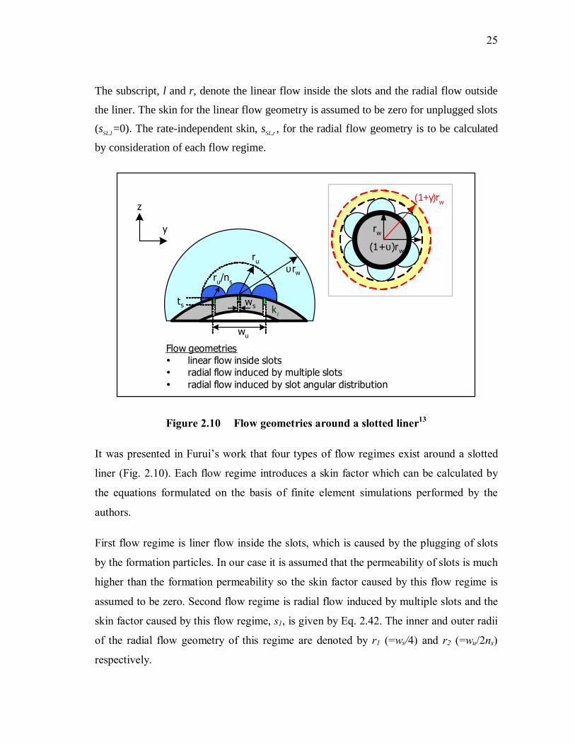
2.5.3 Slotted liner completions

A slotted liner has numerous long and narrow openings (slots) which are milled into the

base pipe to allow fluids to flow into the liner. Slot style is characterized by the

arrangement of the slots around the circumference of the liner (Fig. 2.9).

Furui et al. 13 developed a skin equation for slotted liners which accounts mainly for the

flow convergence to the slots, the slot plugging, effects of formation damage and the

interactions among these effects. In the presence of formation damage around the well

the overall skin is magnified.

Multiplestaggered

Singlestaggered

Multipleinline

Singleinline

wurw

ms

L

ns

λ=ls/lu

ls

lu

wsslot unit

Figure 2.9 Geometric variables for slotted liner skin calculation13

In our case it is assumed that there is no turbulent flow inside the formation which

reduces the rate dependent skin to zero. The skin of a slotted liner is given by,

rSLlSLSL sss ,, += (2.41)

25

The subscript, l and r, denote the linear flow inside the slots and the radial flow outside

the liner. The skin for the linear flow geometry is assumed to be zero for unplugged slots

(sSL,l =0). The rate-independent skin, sSL,r , for the radial flow geometry is to be calculated

by consideration of each flow regime.

Flow geometrieslinear flow inside slotsradial flow induced by multiple slotsradial flow induced by slot angular distribution

rw

(1+υ)rw

(1+γ)rw

ru/ns

ruυrw

wu

ts ws kl

y

z

Figure 2.10 Flow geometries around a slotted liner13

It was presented in Furui’s work that four types of flow regimes exist around a slotted

liner (Fig. 2.10). Each flow regime introduces a skin factor which can be calculated by

the equations formulated on the basis of finite element simulations performed by the

authors.

First flow regime is liner flow inside the slots, which is caused by the plugging of slots

by the formation particles. In our case it is assumed that the permeability of slots is much

higher than the formation permeability so the skin factor caused by this flow regime is

assumed to be zero. Second flow regime is radial flow induced by multiple slots and the

skin factor caused by this flow regime, s1, is given by Eq. 2.42. The inner and outer radii

of the radial flow geometry of this regime are denoted by r1 (=ws/4) and r2 (=wu/2ns)

respectively.

26

+−+−

=

DuDss

DsDs

ss wlnwl

mns

/1/21

ln21 λ

λλ

(2.42)

As it was assumed that the wormholes are considered as infinite conductivity channels

(no pressure drop occurs in the wormholes) so it can be assumed that when the

wormholes cross this regime (i.e. when rwh>r2) the skin factor caused by this flow

regime s1 reduces to zero.

The third flow regime is radial flow induced by the angular distribution of slot units

which exists in the region from r2 (=wu/2ns) to r3 (=υrw). The skin factor caused by this

flow regime is defined by Eqs. 2.43 and 2.44 as,

For high slot penetration ratio (γ<υ),

( ) 2ln/1ln122

++−

=

DsDuDs

s lwl

ms λυλ

λ (2.43)

And for low slot penetration ratio (γ>υ),

+−

+−

=

υλλ

λ 2/1/1

ln22

Ds

DuDs

s lwl

ms (2.44)

where υ and γ are defined by Eqs. 2.45 and 2.46 respectively.

≠≈≠=

15.11)/(

msmsmSin s

υπυ

(2.45)

λ

γ2Dsl

= (2.46)

As the wormhole crosses radius r3 this radial skin component reduces to zero (i.e. s2=0

for rwh> r3).

27

The fourth flow regimes exists due to radial flow away from the liner and it stretches

from radius r3 (=υrw) to r4 (=rb). rb is the distance to a point far away from the center of

the wellbore which has no importance as it ultimately cancels out. The skin factor caused

by this flow regime can be written as s3 and it can be defined by Eqs. 2.47 and 2.48.

For high slot penetration ratio (γ<υ),

)1

ln(3 υ+= Dbr

s (2.47)

And for low slot penetration ratio (γ>υ),

++

−+×

+

+

−−

=

λ

λυυ

λλ

λ

21

ln)1(211

2/ln

)1(2/

3Ds

Db

Ds

Ds

Ds

Dsl

rl

ll

ls (2.48)

In the ideal conditions when there is no fluid path diversion, i.e. all the fluid particles are

following the radial flow pattern from rb to rw. The skin factor s4 can be defined by

Eq. 2.49 as;

)ln(4 Dbrs = (2.49)

The skin for the radial flow geometry, sSL,r , can be calculated by adding s1, s2 and s3 and

by subtracting s4. As the wormhole passes crosses each flow regime the particular skin

factor caused by that flow regime is to be reduced to zero.

When formation damage is present around the wellbore completed with slotted liner the

skin effect is magnified. The change in this skin factor during the wormhole propagation

can be determined using the equations presented in previous section for horizontal wells

with Openhole completions. The complete equations for a slotted liner in presence of

formation damage around the wellbore is given as,

( ) ( ) kksrrkks drSLwdd //ln1/ ,+−= (2.50)

28

2.5.4 Partial penetration skin model

Acid injection in long horizontal wells is often into relatively short, isolated sections of

the well. Because the section treated is connected to the entire reservoir, the injectivity is

higher than it would be if the reservoir ended at the end of the completion interval. A

partial penetration skin factor can be used to account for this effect. This partial

penetration effect is important when injecting into relatively small intervals of horizontal

wells and is not widely recognized, so a brief review is in order. The effect on

productivity of completing a vertical well in only a portion of the reservoir has been

described numerous times, beginning with Muskat15.

Figure 2.11 A section of partially completed vertical wellbore

For a vertical well completed along a thickness, hw, in a reservoir of thickness h

(Fig. 2.11), and in the absence of any other skin effects, the steady-state productivity

index is defined as in Eq. 2.51;

+

=

cw

e srr

B

khJln2.141 µ

(2.51)

Where sc is the partial completion skin factor. When hw is less than h, sc is positive,

accounting for the lessened productivity of the partially completed well. Models to

calculate sc have been presented in many studies, including those of Cinco-Ley et al.16,

h

Zw

hw

hw = Completion thickness Zw = Elevation

rw

29

Odeh17, and Papatzacos18. The productivity index could also be written using the

completed thickness in the inflow equation;

+

='ln2.141 c

w

e

w

srr

B

khJ

µ (2.52)

If hw is less than h, sc’ must necessarily be negative to give the same productivity index

as Eq. 2.51. When hw is relatively small compared with h, these partial completion

effects are large. For example, when hw/h is 0.25, sc is 8.8 using the Papatzacos model

when the completion is centered in an isotropic reservoir. If ln(re/rw) is 8, a typical

value, the corresponding sc’ is -3.8. Thus, when calculating productivity or injectivity

based on the completion zone thickness, the well appears to be stimulated because the

reservoir is thicker than the completed interval.

Figure 2.12 Horizontal well partially open to the reservoir

open section2a

L

h rw

30

Figure 2.13 Ellipsoidal flow geometry

The corresponding situation for acid injection into a short interval of a horizontal well is

shown in Fig. 2.12. Because we are assuming radial flow from the completed interval in

our reservoir flow model, there will be a large partial penetration effect which we can

account for with a negative skin factor.

A simple model is developed to calculate this type of skin factor as follows. Consider a

horizontal well partially open to the reservoir as in Fig. 2.12. Ellipsoidal flow exists due

to partial opening of wellbore in the reservoir as in Fig. 2.13. If the formation is isotropic

then in prolate spherodial coordinates the pressure drop can be given by; *

−

+=∆1

1ln)2(

2.141ξ

ξµe

eakq

p (2.53)

where )(sinh 1

Dr−=ξ (2.54)

arrD /= (2.55)

The radial flow equation based on a completed interval of length 2a is

+

=∆ pp

ws

rr

akqp ln)2(

2.141 µ (2.56)

*Personal communication for horizontal well partial penetration skin with K.Furui, ConocoPhillips, A.D.Hill, and D.Zhu, Texas A&M U., College Station, TX (2007).

r

+a-a

31

We can calculate the pseudo-skin factor due to ellipsoidal flow to the open section. For a

centered well, r=h/2 (i.e. rD=r/a=h/2a) in Eq. 2.56. Equating the pressure drops given by

Eqs. 2.53 and 2.56 provide the horizontal well partial penetration skin factor as,

++−

+++=

−

+=

+

=

−+

)11(

)11(2ln

)1(

)1(2ln

2ln

11ln

2

2

DD

DDwwpp

ppw

rrh

rrr

eh

ers

srh

ee

ξ

ξ

ξ

ξ

(2.57)

The partial penetration skin is calculated using Eq. 2.57 and it will be accounted in the

total skin factor. This partial penetration skin factor is added to the skin factor calculated

from formation damage skin and completion skin models. The overall skin factor is used

in the reservoir flow model equation to obtain the solution. It is noted that the partial

penetration skin factor remains constant during the matrix acidization process.

2.5.5 Solution of matrix acidizing model

To solve the problem of matrix acidization in a horizontal well, all presented models are

integrated and solved in a discretized manner in time and space. Initial and boundary

conditions to solve this system of equations are defined as;

Lxtxqpxp

xq

w

Rw

w

≥===

;0),()0,(

0)0,( (2.57)

The first and second condition explain that the initial wellbore flow rate at any point is

zero (i.e. qw=0) as the wellbore pressure is equal to the reservoir pressure (i.e. pw = pR).

The third condition explains that there is no lateral flow in the wellbore beyond the toe

of the well (i.e. x>L). Along with these initial and boundary conditions the injection rate

at the heel of the well (i.e. x=0) is defined as in Equation 2.58;

)(),0( tqtq iw = (2.58)

32

In summary, the steps to solve the model equations are as follows:

1. Divide the horizontal wellbore into small segments.

2. Divide the injection time into small time steps.

3. Apply the initial and boundary conditions.

4. Use the skin model to get the skin factors for each segment (Section 2.5).

5. Solve the pressure drop equation (Eq. 2.5) and the reservoir flow equation

(Eq. 2.9) to get pw, qw, and qr.

6. Use the interface tracking model (Eq. 2.14) to get the interface locations (xint).

7. Calculate the volume of acid injected into each segment during the time step

from the flow distribution and interface locations.

8. Use the wormhole model to get the length of wormholes in each segment at the

end of the time step (Section 2.4).

9. Go back to step 4 and loop through the skin factor calculation using new

wormhole length.

33

CHAPTER III

MATRIX ACIDIZING SIMULATOR

3.1 Matrix acidizing simulator

The models for wellbore flow, partial penetration and completion skin factor, front

tracking, reservoir inflow, wormhole growth, and skin evolution are incorporated

together to obtain the solution of acidizing in a horizontal well. To achieve this wellbore

is divided into small segments and equations for wellbore material balance, wellbore

pressure drop and reservoir inflow needs to be written in discretized form. As stated in

Chapter II initial and boundary conditions are applied to solve the equations.

A simulator is developed implementing all the models and solution scheme described in

APPENDIX A. The simulator implements the theoretical models developed in this study.

The models determine the volume of acid injected (bbl/ft) as a function of position along

the wellbore by tracking the movement of the acid in the wellbore and the formation. For

matrix acidizing treatments, the model also predicts the depth of penetration of

wormholes as a function of position along the zone. Skin factor is calculated after

wormhole length is obtained from the wormhole models. Pressure, injection rate,

wormhole length and skin factor distribution along the injection intervals of the well will

be the final output of the simulator.

The acid placement simulator model equations are developed in FORTRAN-90. The

simulator reads the data from the input data file. This input data file contains the

information about the well completion and reservoir properties along the length of

wellbore. A sample input data file is shown in APPENDIX B.

The simulator also provides bottomhole pressure at the heel as output for a defined

injection rate schedule. This simulated pressure can be used as a tool to analyze the past

treatments for which the observed bottomhole pressure data are available.

34

3.2 Simulator data files

The input data file contains the information about the well completion and reservoir

properties along the length of wellbore. The output data files contain the calculated

values of the various parameters. A list of various files used by the simulator is given in

Table 3.1.

Table 3.1 Matrix acidizing simulator data files

DATA FILE TYPE FILE INFORMATION

data.acm Input file Contains well completion, reservoir data, and acid treatment data

pwheel.acm Output file Pressure history at the heel of the well

qwheel.acm Output file Injection rate history at the heel of the well

pgauge.acm Output file Pressure history at the surface gauge

stot.acm Output file Total skin factor history

pindex.acm Output file Productivity index history

pw.acm Output file Injection pressure in each grid block at the end of each stage

qsr.acm Output file Specific injection rate in each grid block at the end of each stage

vinj.acm Output file Injected acid volume in each grid block at the end of each stage

skin.acm Output file Skin factor in each grid block at the end of each stage

lwh.acm Output file Wormhole length in each grid block at the end of each stage

pvbt.acm Output file Pore volume for break through in each grid block at the end of each stage

3.2.1 Input data file

The input file (data.acm) contains the information about the well completion, reservoir

properties and acid treatment. A sample input data file for the simulator is presented in

APPENDIX B. The comments lines starts with dash and are provided as a help to

facilitate the input data entry. It contains four sections separated by different keywords.

35

The first section starts with the keyword %WRC and it contains information of well

completion and reservoir properties. The casing and tubing diameter are defined in this

section. The number of grid cells required in a horizontal well is also defined in this

section and property of each grid block such as grid block length, porosity, permeability,

perforation details, initial damage; initial damage radius etc can be defined individually.

The next section starts with the keyword %INJ and it contains the injection treatment

information. The boundary condition needed for the solution is defined as constant rate

or constant pressure. The injection rate schedule is to be defined in case of constant rate

boundary condition to get the simulated pressure at the heel as output. The pressure

values at different time step can be supplied as input to the simulator in case of constant

pressure boundary condition. The next section starts with the keyword %IFP and the

injected fluid information is given as input. This section provides a tool to handle the

injection of multiple fluids such as water, acid etc. The selection of wormhole model is

facilitated with the help of next section which starts with the keyword %WHM. The

volumetric wormhole model needs the pore volume for breakthrough (PVbt) as input. For

Buijse’s semiempirical model two inputs are needed which are optimum pore volume for

breakthrough (PVbt-opt) and optimum injected fluid velocity (Vi-opt). Irrespective of the

selected wormhole model these input parameters are determined from the core flow

experiments performed in the lab. The input data file end with the keyword %END

which tells the simulator that it has reached the end of the file and the input data reading

process terminates.

3.2.2 Output data files

Table 3.1 provides a detailed list of various output data files of the simulator. The output

of acid placement simulator includes the skin, wormhole length, acid coverage along the

length of the wellbore at changing time steps. It provides the variation of bottomhole

pressure, injection rate, and productivity index with time. The location of fronts created

between several injected fluids is also included in output. The output files generated

from the FORTRAN program can be opened with the notepad. The output data from

these files can be edited in MS Excel for output data processing.

36

CHAPTER IV

RESULTS

A set of simulations were performed using the acidizing simulator for long horizontal

wells. These results provide a better understanding of how acid is distributed in a

wellbore. It is also analyzed that how well and reservoir parameters affect the results.

The output of the hypothetical cases and study of an actual treatment are presented in

this chapter.

4.1 Hypothetical examples

In these examples, the effects of acid volume and acid injection rate on the placement of

injected acid and the resulting distribution of acid along the well are investigated. The

completion of horizontal well affects the acidizing performance. Matrix acidizing in

openhole completions, cased-perforated completions, and slotted liner completions are

discussed separately in different subsections.

4.1.1 Horizontal well with openhole completion

In this example, acid is injected at a relatively low rate into a long section of a horizontal

well. This is the situation where wellbore flow conditions are most likely to be

significant. The conditions for this case are presented in Table 4.1. A uniform

distribution of permeability, porosity, initial damage ratio, and initial damage radius

along the length of the wellbore is assumed. The volumetric model of wormhole growth

was used in the acidizing simulator to model the wormhole growth.

Assuming that the acid is being injected from a tubing tail located at one end of the

completed interval, the progression of acid placement with time is shown in Fig. 4.1. By

the end of 200 barrels of acid injection at 100 minutes of pumping time, acid has not yet

reached the far end of the completed interval. For better acid coverage with this small

volume treatment (the total volume pumped in 100 minutes is only 8.4 gal/ft), some

method of diversion is required.

37

Table 4.1 Data for acid injection into horizontal well with openhole completion

Well length 1000 ft

Number of grid blocks 50

Grid block length 20 ft

Completion Open hole

Damage radius 0.5 ft

Permeability 2 md

Index of anisotropy 1

Permeability impairment ratio 0.5

Reservoir rock Limestone

Acid 15 % Hcl

Reservoir pressure 3200 Psi

Wormhole model Volumetric

Pore volume for breakthrough (PVbt) 2

Injection rate 2 bpm

Duration of pumping 100 Min

The distribution of wormhole lengths along the wellbore created by this acid injection is

shown in Fig. 4.2. By 100 minutes of acid injection, wormholes had extended 6 inches

into the formation at the heel of the completed interval. Injection of larger volumes of

acid improves the coverage of acid in this long interval. With 500 bbl of acid injected,

the far end of the completed interval has received a significant amount of acid injection,

with good acid coverage along most of the interval (Fig. 4.3). For a well with only minor

damage, as was assumed for this case, although the acid is increasing the local

injectivity, and thus retarding the progress of the acid down the wellbore, the injectivity

is changing slowly, and thus does not have a strong effect on the acid placement.

Another illustration of this is obtained by changing the efficiency of the acid treatment

by changing the PVbt parameter used in the volumetric model. Fig. 4.4 compares the acid

placement for cases ranging from PVbt of 0.5 (very rapidly propagating wormholes) to

inert fluid (no wormholes, hence no change in injectivity during injection). The acid

38

coverage changes a little depending on how efficiently the acid is increasing injectivity

of the formation, but it is not a large effect. One of the interesting predictions of this

model is the downhole pressure response during acid injection. Bottomhole pressure

measurements are becoming more and more common during acid injection and can

provide very useful diagnostic information about the treatment. The predicted pressure

responses for a wide range of PVbt are shown in Fig. 4.5. When an inert fluid is injected,

the pressure builds up because of the transient nature of the reservoir flow. With acid

injection, the simultaneous stimulation is tending to decrease the injection pressure.

Thus, depending on how efficiently the acid is increasing the near-well permeability, the

injection pressure may rise or fall, as shown in Fig. 4.5. Comparison of actual treatment

response with predictions like these provide a means of diagnosing the effectiveness of

acid stimulation and if done in real time can be used to optimize a treatment on the fly.

The final aspect of this hypothetical case is the effect of the wormhole model on the

predicted acid placement. With the Buijse model, the wormhole propagation is varying

with acid flux, with the maximum wormhole propagation being at the optimal injection

condition. In this particular case, the acid fluxes are near the optimum, but somewhat

higher. For the range of acid fluxes occurring in this treatment, the PVbt from the Buijse

model varies from about 2 to about 2.5 (Fig.4.6). Fig. 4.7 shows the wormhole length

distribution from the volumetric model with PVbt set to 2.5 compared with the predicted

placement using the Buijse model with the PVbt-opt equal to 1.5. The volumetric model,

which assumes a constant PVbt independent of acid flux, gives a similar prediction of

acid placement, and hence, wormhole distribution, when a value of 2.5 was used for PVbt.

39

Figure 4.1 Acid coverage over the entire length of wellbore

Figure 4.2 Wormhole length distributions at different times

0.00

0.05

0.10

0.15

0.20

0.25

0 200 400 600 800 1000Position along well (ft)

Aci

d vo

lum

e (b

bl/ft

)

10 min

40 min

80 min

100 min

0.00

1.00

2.00

3.00

4.00

5.00

6.00

7.00


Wor

mho

le le

ngth

(in)

10 min

40 min

80 min

100 min

40

Figure 4.3 Acid placement profiles for 200 and 500 bbls of acid

Figure 4.4 Acid placement profiles for different values of PVbt

0.00

0.10

0.20

0.30

0.40

0.50

0.60

0 200 400 600 800 1000

Position along well (ft)

Aci

d vo

lum

e (b

bl/ft

)500 bbls acid (21 gal/ft)

200 bbls acid (8.4 gal/ft)

0.00

0.05

0.10

0.15

0.20

0.25

0.30


Aci

d vo

lum

e (b

bl/ft

)

PVbt=0.5PVbt=2

PVbt=10Inert fluid

41

Figure 4.5 Pressure responses during acid injection

Figure 4.6 PVbt versus Vi during simulation using Buijse Model with PVbt-opt=1.5

3100

3200

3300

3400

3500

3600

3700

3800

0 20 40 60 80 100 120Time (min)

Pre

ssur

e (p

si)

PVbt=0.5

PVbt=2

PVbt=10

Inert fluid

0.1000

1.0000

10.0000

0.0100 0.1000 1.0000 10.0000

Interstitial fluid velocity, Vi (cm/min)

PVbt

42

Figure 4.7 Comparison of wormhole distributions from the volumetric and

Buijse’s models

4.1.2 Horizontal well with cased-perforated completion

It is described in the Chapter II that skin factor evolution in cased-perforated

completions is different from the openhole completions. The increase in the length of

wormhole is added to the perforation length at the end of time step to calculate the new

perforation length. This new perforation length is provided to the skin model to calculate

the new skin factor at the end of time step. The data used in simulating the results for

this case is presented in Table 4.2.

In this example, the perforation length varies from 9 to 13 inches from heel to toe of the

well. The distribution of perforation length along the length of wellbore is shown in Fig.

4.8. This variation in length is adopted as Gdanski referred in his work that by having

higher injectivity at the toe helps in achieving a uniform coverage of the acid. The part

of wellbore lying towards the toe receives less acid when compared to the part of the

wellbore lying towards the heel. By putting longer perforations towards the toe of the

well would certainly results in a better stimulation.

0.00

1.00

2.00

3.00

4.00

5.00

6.00


Wor

mho

le le

ngth

(in)

Buijse's Model for PVbt-opt = 1.5

Volumetric model for PVbt = 2.5

43

Table 4.2 Data for acid injection into horizontal well with cased-perforated

completion

Well length 1000 ft No. of grid blocks 50 Grid block length 20 ft Completion Cased perforated Damage radius 1 ft Permeability impairment 0.5 Permeability 2 md Index of Anisotropy 1 reservoir rock Limestone Acid 15% Hcl reservoir pressure 3200 Psi wormhole model Volumetric PVbt 3 injection rate 2 bpm duration 100 min

Perforation data mp 2 Perforation length (lp) 9-13 inches dp= 0.3 inches Np= 1 spf α= 90 degree Rkcz=kcz/k= 1 dcz= 0.0003 inches

The simulations results for the above data are shown in Figs. 4.9 - 4.12. In Fig. 4.9, the

evolution of skin is shown at different time steps of 10 min, 40 min, 80 min, and 100

min. The skin is less in those areas which have long perforation lengths (i.e. towards the

toe). In Fig. 4.10 the acid coverage along the length of the wellbore is shown and it is

increasing towards the toe. The acid coverage supports the claim that putting longer

perforations towards the toe of the well improves acid coverage. The part of the wellbore

towards the toe has received more acid thus an improved stimulation. Fig. 4.11 presents

the distribution of wormholes along the length of the wellbore. It is evident from this

figure that the wormhole distribution imitates the acid coverage pattern. Fig. 4.12 shows

a comparison between two cases i.e. acid injection into a horizontal lateral with uniform

44

and non-uniform distribution of perforation length. It can be concluded that by putting

the longer perforation at the toe of the well certainly would place the acid in the parts of

the wellbore which need stimulation e.g. the area towards the toe of the wellbore.

Figure 4.8 Distribution of perforation length along the wellbore

Figure 4.9 Evolution of skin with time during acid injection

0

2

4

6

8

10

12

14


Perf

orat

ion

leng

th (i

n)

0.00

1.00

2.00

3.00

4.00

5.00

6.00

7.00

0 200 400 600 800 1000


Skin

(dim

ensi

onle

ss) 10 Min

40 Min80 Min100 Min

45

Figure 4.10 Acid coverage in cased-perforated completion case

Figure 4.11 Distribution of wormholes in cased-perforated completion case

0.000.020.040.060.080.100.120.140.160.180.20


Aci

d vo

lum

e (b

bl/ft

)

10 Min

40 Min

80 Min

100 Min

0.000.200.400.600.801.001.201.401.60

0 200 400 600 800 1000


Wor

mho

le le

ngth

(in)

10 Min

40 Min

80 Min

100 Min

46

Figure 4.12 Comparison of acid coverage in uniform and non-uniform

perforation length distribution

4.1.3 Horizontal well with slotted liner completion

The horizontal well can be completed with slotted liners in unconsolidated formations. It

is described in Chapter II that various flow regimes exists around the slotted liner. Each

flow regimes causes an additional pressure drop which can be quantified as skin factor.

In carbonate formations wormhole crosses through each flow regime reducing the skin

factor caused by each flow regime. The statement is true as wormholes are considered as

infinite conductivity channels. A simulation was made using the data presented in

Table 4.3.

Figures 4.13 and 4.14 show the wormhole length distribution and skin distribution at

different time steps respectively along the wellbore. In presence of formation damage

around the slotted liner the overall skin magnifies and it can be seen from the Fig. 4.14

that s=3.2 in the parts of the wellbore which are not stimulated. It was explained in

Chapter II that a second flow regime is caused by multiple slots exists from region r1 to

r2. In this case r2=wu/2ns= 0.25 inches. There is a drop in skin factor for when the

0.00

0.05

0.10

0.15

0.20

0.25


Aci

d vo

lum

e (b

bl/ft

)

Acid coverage with uniform perforation length of 9 inches

Acid coverage with variable perforation length

47

wormhole length crosses this region (i.e. >r2). Furthermore there exists a flow regime

extending from r2 to r3 where r3= νrw=0.91 inches. It is evident from Fig. 4.14 that the

skin factor takes a further drop in all those zones where the wormhole length has crossed

the third flow regime (i.e. r3). The formation of wormhole might overcome the

completion skin caused by various flow regimes around a slotted liner. Matrix acidizing

can be used as a tool to enhance the productivity from the horizontal wells completed

with slotted liners.

Table 4.3 Data for acid injection into a horizontal well with slotted liner

completion

Well length 1000 ft No. of grid blocks 50 Grid block length 20 ft Completion Slotted liner Damage radius 0.5 ft Damage impairment 0.5 Permeability 2 md Index of Anisotropy 1 reservoir rock Limestone Acid 15% Hcl reservoir pressure 3200 Psi wormhole model Volumetric PVbt 3 injection rate 2 bpm duration 30 min

Slotted liner data ms 12 Os 0.059 ns 2 ws 0.5 inches ls 2 inches

48

Figure 4.13 Distribution of wormhole length in slotted liner completion

Figure 4.14 Distribution of skin in slotted liner completion

0.00

0.50

1.00

1.50

2.00

2.50


Wor

mho

le le

ngth

(in)

10 Min

20 Min

30 Min

r2=0.25

r3=0.91

0.00

0.50

1.00

1.50

2.00

2.50

3.00

3.50

0 200 400 600 800 1000


Skin

(dim

ensi

onle

ss)

10 Min 20 Min

30 Min

Skin in unstimulated portionDrop in skin as rwh>r2

Drop in skin as rwh>r3

49

4.1.4 Heterogeneity effect in horizontal well acidizing

When using long horizontal well in carbonate reservoirs with heterogeneous reservoir

properties along the length of wellbore, most of these wells often encounter thief zones

(zones of high permeability. These zones can consume much of the injected acid during

the treatment thus affecting the overall acid distribution. It is planned to study the effect

of acid injection into the wells with thief zones. The data used in this case is listed in

Table 4.4.

The initial damage and permeability is varying along the length of wellbore and their

distribution is shown in Figs. 4.15 and 4.16. Buijse’s model is used in simulation and it

provides a decrease in wormhole growth rate with respected to increasing wormhole

length. The wellbore encounters three thief zones which are located at 1000 ft, 2000 ft,

and 3000 ft from the heel of the wellbore.

Table 4.4 Data for acid injection into a horizontal well with thief zones

Well length 4000 ft No. of grid blocks 200 Grid block length 20 ft Completion Openhole Permeability 2-8 md Permeability impairment ratio 0.5 Index of Anisotropy 1 Reservoir rock Limestone Acid 15% Hcl Reservoir pressure 3200 Psi Wormhole model Buijse PVbt-opt 1.5 Vi-opt 0.1 cm/min Injection rate 20 bpm

Details for thief zones Location 1000,2000,3000 ft Length 20 ft Permeability 1000 md

50

Figure 4.15 Distribution of initial damage along the length of wellbore

Figure 4.16 Distribution of permeability along the length of wellbore

00.5

11.5

22.5

33.5

44.5

5

0 1000 2000 3000 4000


Intia

l dam

age

radi

us (f

t)

1

10

100

1000

0 1000 2000 3000 4000


Perm

eabi

lity

(md)

51

The acidizing treatment has been continued until the 100 gal/ft (9523 bbl injected acid

volume). It has been observed that each thief zone consumed approximately 4500 gal/ft

of injected acid, and the rest of the well has received approximately 31 gal/ft of injected

acid which is sufficient to propagate the wormholes through the damaged zone. Fig. 4.17

shows a plot of acid coverage along the length of wellbore comparing two situations at

different time steps. It shows from Fig. 4.17 that at the end of the injection, most of the

wellbore receives uniform acid coverage. The acid coverage volume is high in zones of

high permeability, and is low in zones of low permeability. The distribution of

wormholes imitates the acid coverage curve. The injectivity index from the start to end

of the job is shown in Fig. 4.18 which indicates that after the initial decrease the PI starts

increasing sharply and maintains a flat trend after 250 minutes of injection. Fig. 4.19

shows local skin factors at the end of simulation. Even though at the end of the treatment,

the most of the wellbore received sufficient acid, without thief zones, the uniform acid

distribution can be achieved much faster than the shown case. It is realized that the thief

zones that take most of the injected acid should not be treated (due to high permeability),

diversion is obviously necessary in such cases.

Figure 4.17 Acid coverage along the length of wellbore

0

20

40

60

80

100

0 1000 2000 3000 4000Position along well (ft)

Aci

d Vo

lum

e (g

al/ft

)

952 bbls of acid injected (10 gal/ft)

9523 bbls of acid injected (100 gal/ft)

52

Figure 4.18 Injectivity index during the acid injection

Figure 4.19 Local skin factors along the wellbore at the end of simulation

0

50

100

150

200

250

0 100 200 300 400 500

Time (min)

Inje

ctiv

ity in

dex

(bbl

/day

/psi

)

-4.00-3.50-3.00-2.50-2.00-1.50-1.00-0.500.00

0 1000 2000 3000 4000


Ski

n (d

imen

sion

less

)

53

4.2 Field study

In this field study, predictions for an actual North Sea horizontal well completed in a

chalk formation are presented. It is a case where short intervals of the wellbore are

treated with the high volume of acid. The 6000-ft long horizontal well was completed

with sixteen individual 10 foot-long perforated intervals spaced along the well. Each

interval is perforated with one shot per foot with the perforations oriented downward. In

this stimulation treatment, each zone was isolated with packers (Fig. 4.20) and

individually treated with 15% HCl. The treating string was equipped with pressure

gauges between the packers and on either side of the packers enabling the operator to

monitor the downhole treating pressure and to determine if the packers were set and not

leaking. We used our acid placement model to history match the treating pressure

response for one of the zones treated.

Figure 4.20 Selective stimulation for each perforated zone using straddle

packers and perforated coiled tubing

The pressure records from the three downhole gauges are shown in Fig. 4.21. There is a

clear indication of the packers being set. The pressure gauge on the heel side of the first

packer shows no pressure response to injection, indicating that the isolation has been

established.

54

Figure 4.21 Pressure response of downhole gauges

Figure 4.22 Rate schedule for North Sea field well acid treatment simulation

0100020003000400050006000700080009000

10000

0 10 20 30 40 50Time (min)

Pres

sure

(psi

)

BHP-ZoneBHP-BelowBHP-Above

Isolation of bottom zone achieved

Isolation of top zone achieved

Start of acid injection in the formation

0

2

4

6

8

10

12

14

16

0 10 20 30 40 50Time (min)

Inje

ctio

n ra

te (b

pm)

Treatment rateSimulated rate

zonal isolation achieved at 6 bpmPzone=9050 Psi

Acid Injection Startedat 5 bpm

Response of the whole well (packers are not set)

Acid injection stopped

55

Then at about 22 minutes, the second packer was set, as indicated by the rapid pressure

falloff recorded by the gauge beyond the second packer. It was decided to start the

simulation treatment at the 22 minute, when both packers were set and acid injection into

the isolated interval began. To history match the pressure response during this treatment,

the actual injection rate schedule recorded is provided as input to the acid placement

simulator. Fig. 4.22 shows how the approximation of the changing rate schedule as a

series of discrete changing rate is done. Additional data used in the model is given in

Table 4.5.

Table 4.5 Input data for North Sea field well

Casing ID 6.625 inches Coiled tubing OD 2.55 inches Pipe roughness 0.0001 Zone length 10 ft Reservoir pressure in zone 5350 psi Reservoir compressibility 5E-06 psi-1 Permeability 5 md Porosity 0.38 Initial formation damage none Perforation length 7 inches Perforation diameter 0.264 inches Perforation spacing 1 spf Perforation phasing 0 degree Perforation orientation 90 degree Acid type HCl Acid density 69.91 lbm/ft3

Acid viscosity 1 cp Acid concentration 15% Wormhole model Volumetric Number of grid blocks 10 Reservoir thickness 200 ft

56

The skin factor model is presented in Chapter II. From the data given about the well, the

initial skin factor can be calculated as follows. For the given perforating conditions, a

perforation skin factor of 4.6 is obtained using the Furui et al. model.13 For this very

short interval in a large reservoir, a partial penetration skin factor of -5.5 is obtained with

Eq. 2.57. Combining these, and assuming no formation damage was present initially, an

initial total skin factor of -0.9 is used. It is decided to adjust the reservoir permeability

and the PVbt in the volumetric model to obtain a match of the actual treating pressure

(Fig. 4.23). This match was obtained by setting the PVbt to 4.5, which means the acid is

propagating wormholes relatively slowly into the matrix and that a large volume of rock

is being dissolved in the treated region. With PVbt of 4.5, the wormhole front is moving

4.5 times slower than the injected fluid (spent acid) front.

For the high rate injection into such a short interval, acid placement is not an issue, as

shown in Fig. 4.24. What more important for this type treatment is the effects of this

large volume acid treatment from the predicted depth of acid penetration into the

formation. Notice that this interval has received 120 barrels of acid, about 500 gal/ft.

Figure 4.23 History match of treatment pressure

0100020003000400050006000700080009000

10000

0 20 40 60 80Time (min)

Pres

sure

(psi

)

Treatment pressureSimulated pressure

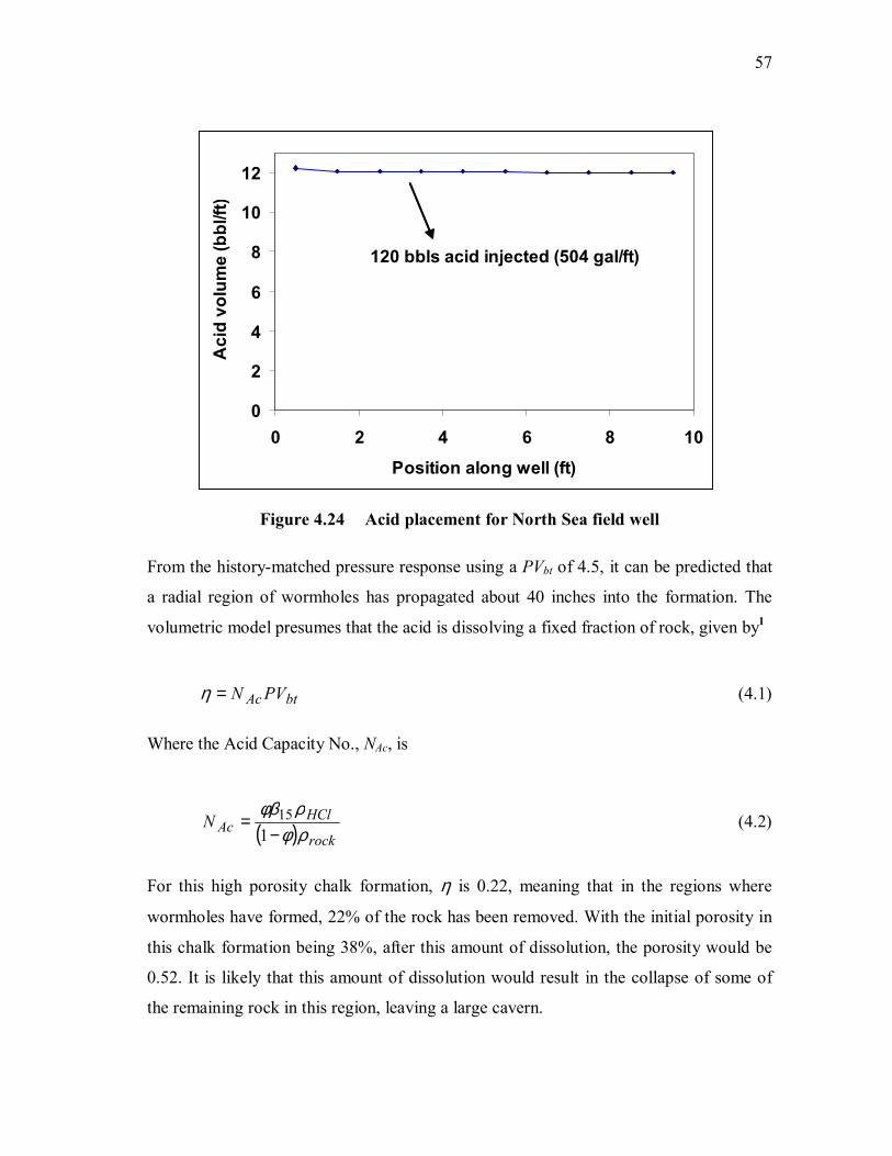
57

Figure 4.24 Acid placement for North Sea field well

From the history-matched pressure response using a PVbt of 4.5, it can be predicted that

a radial region of wormholes has propagated about 40 inches into the formation. The

volumetric model presumes that the acid is dissolving a fixed fraction of rock, given by1

btAc PVN=η (4.1)

Where the Acid Capacity No., NAc, is

( ) rock

HClAcN

ρφρφβ

−=

115 (4.2)

For this high porosity chalk formation, η is 0.22, meaning that in the regions where

wormholes have formed, 22% of the rock has been removed. With the initial porosity in

this chalk formation being 38%, after this amount of dissolution, the porosity would be

0.52. It is likely that this amount of dissolution would result in the collapse of some of

the remaining rock in this region, leaving a large cavern.

0

2

4

6

8

10

12

0 2 4 6 8 10


Aci

d vo

lum

e (b

bl/ft

)

120 bbls acid injected (504 gal/ft)

58

Based on the dissolving power of 15 % HCl reacting with calcite, 12 bbl of acid

injection into a single perforation will dissolve 5.5 ft3 of solid. Assuming that the

dissolution region extends 40 inches from the wellbore, as predicted by the volumetric

model with PVbt = 4.5 as used in this history match, the acid has likely dissolved a

sufficient amount of rock out to at least this distance to make the remaining rock

unstable.

59

CHAPTER V

CONCLUSIONS

5.1 Conclusions

An acidizing model has been developed for horizontal wells in carbonate reservoirs,

which incorporates a wellbore flow model, an interface tracking model, a wormhole

model to predict the effect of the acid injection on local injectivity, a skin evolution

model that combines the stimulation effect of the acid with other skin effects, and a

transient reservoir inflow model. With this model, it was found that

o Small volume treatments in long horizontal intervals result in non-

uniform acid placement, but that the placement improves with increasing

acid volume;

o In horizontal wells completed with slotted liners, matrix acidizing might

overcome the high completion skins, as wormholes pass through the flow

convergence zones;

o Partial penetration effects are important when injecting into relatively

short intervals of long horizontal wells;

o The parameters in a wormholing model can be adjusted to history match

(or predict) the pressure response of an acid treatment in a horizontal

well;

o History matching of an acid treatment in a North Sea well completed in a

chalk formation required a relatively high value of the pore volumes to

breakthrough parameter, suggesting that the acid is propagating slowly

into the rock, creating a cavity around the wellbore.

60

REFERENCES

1. Economides, M. J., Hill, A. D., and Ehlig-Economides, C.: Petroleum

Production Systems, Prentice Hall, Englewood Cliffs, NJ, 1994.

2. Rae, P. and Di Lullo, G.: “Matrix Acid Stimulation – A Review of the State-of-

the-Art,” paper SPE 82260 presented at the 2003 SPE European Formation

Damage Conference, The Hague, 13-14 May.

3. Jones, A. T. and Davies, D. R.: “Quantifying Acid Placement: The Key to

Understanding Damage Removal in Horizontal Wells,” paper SPE 31146

presented at the 1996 SPE Formation Damage Control Symposium, 14-15

February, Lafayette, Louisiana.

4. Buijse, M. and Glasbergen, G.: “Improved Acid Diversion Using a Placement

Simulator,” paper SPE 102412 presented at 2006 SPE Russian Oil and Gas

Technical Conference and Exhibition, Moscow, Russia, October 3-6.

5. Eckerfield, L. D., Zhu, D., Hill, A. D., Thomas, R. L., Robert, J. A., and Bartko,

K.: “Fluid Placement Model for Horizontal-Well Stimulation,” SPE Drilling &

Completions, (September 2000) 15, No. 3.

6. Gdanski, R.: “Recent Advances in Carbonate Stimulation,” paper IPTC 10693

presented at the 2005 International Petroleum Technology Conference, 21-23

November, Doha, Qatar.

7. Bazin, B., Charbonnel, P., and Onaisi, A.: “Strategy Optimization for Matrix

Treatments of Horizontal Drains in Carbonate Reservoirs, Use of Self-Gelling

Acid Diverter,” paper SPE 54720 presented at the 1999 SPE European Formation

Damage Conference, The Hague, 31st May-1st June.

8. Mitchell, W.P., Stemberger, D., and Martin, A.N.: “Is Acid Placement Through

Coiled Tubing Better Than Bullheading?,” paper SPE 81731 presented at the

2003 SPE/ICoTA Coiled Tubing Conference, Houston, Texas, 8-9 April.

61

9. Lee, J., Rollins, J.B., and Spivey, J.P.: Pressure Transient Testing, SPE Textbook

Series, Vol. 9, SPE, Richardson, Texas (2003).

10. Fredd, C.N., and Miller, M.J.: “Validation of Carbonate Matrix Stimulation

Models,” paper SPE 58713, presented at the 2000 SPE International Symposium

On Formation Damage Control, Lafayette, LA, February 23-24, 2000.

11. Hill, A. D., Zhu, D., and Wang, Y.: “The Effect of Wormholing on the Fluid-

Loss Coefficient in Acid Fracturing,” SPE Production and Facilities, (November

1995) 10, No. 4.

12. Buijse, M. and Glasbergen, G.: “A Semiempirical Model to Calculate Wormhole

Growth,” paper SPE 96982 presented at 2005 SPE Annual Technology

Conference, Dallas, Texas, October 9-12.

13. Furui, K., Zhu, D., and Hill, A.D.: “A Comprehensive Skin-Factor Model of

Horizontal-Well Completion Performance,” SPE Production and Facilities,

(August 2005) 20, No. 3.

14. Karakas, M., and Tariq, S.M.: “Semianalytical Productivity Models for

Perforated Completions, “ SPEPE (February 1991), 73-82.

15. Muskat, M.: Flow of Homogeneous Fluids Through Porous Media, McGraw Hill

Book Co., New York, (1937).

16. Cinco-Ley, H., Ramey, H. J., Jr., and Miller, F. G.: “Pseudoskin Factors for

Partially-Penetrating Directionally-Drilled Wells,” paper SPE 5589 presented at

the SPE-AIME Annual Conference, Sept. 28-Oct. 1, 1975, Dallas, Texas.

17. Odeh, A. S.: “An Equation for Calculating Skin Factor Due to Restricted Entry,”

JPT, (June 1980,) 964-965.

18. Papatzacos, P.: “Aproximate Partial-Penetration Pseudoskin for Infinite-

Conductivity Wells,” SPE Reservoir Engineering, (May 1987,) 227-234.

62

NOMENCLATURE

a = half length of open interval, ft

aj = parameter in inflow equation, bbl/min-psi

am = correlation constant for s2D

A = cross-sectional area of wellbore, ft2

Ai = coefficients in solution matrix

bj = parameter in inflow equation, bbl/min

bm = correlation constant for swb

B = B-function in Buijse’s model

Bi = coefficients in solution matrix

cm = correlation constant for swb

ct = total compressibility, psi-1

Ci = coefficients in solution matrix

d = internal diameter of wellbore, ft

dm = correlation constant for s3D

em = correlation constant for s3D

ff = fanning friction factor, dimensionless

fm = correlation constant for s3D

gm = correlation constant for s3D

h = reservoir thickness, ft

hi= interval height (perforations), m

hp = perforation spacing, spf

hw = length of completed interval, ft

J = productivity index, bbl/day/psi

k = permeability of reservoir rock, md

K = coefficient matrix

63

kcz = permeability of crushed zone, md

kd = permeability of damaged region, md

k• = permeability inside slot, md

l = length of reservoir segment, ft

lDs = dimensionless slot width, dimensionless

lp = perforation length, inches

lp,eff= effective perforation length, inches

lps = damage length covering over a perforation, inches

lpD= dimensionless perforation length, dimensionless

ls = slot length, inches

lu = slot unit length, inches

L = length of wellbore, ft

ms= num. of slot units around the circumference of the liner

mp= num. of perforations around the circumference of the casing

ns= num. of slots per slot unit

NAc = acid capacity number, dimensionless

NRe = Reynolds number, dimensionless

Os= Fraction of open area in a slotted liner

pD = dimensionless pressure

pR= initial reservoir pressure, psi

pw = pressure at any point in the wellbore, psi

pwf = wellbore flowing pressure at heel, psi

PVbt = pore volume for break through, dimensionless

PVbt-opt = optimum PVbt, dimensionless

qi = injection rate at heel, bbl/min

qR = reservoir inflow rate per unit length of wellbore, bbl/min/ft

64

qw = wellbore flow rate at any point, bbl/min

∆q = change in rate, bbl/min

Q = volumetric flow rate (Buijse’s model), m3/s

r = radius, m

rb= outer boundary radius, ft

rcz= radius of crushed zone, ft

rd = radius of damaged zone, ft

rD= dimensionless radius

re = reservoir drainage radius, ft

rp= perforation radius, inches

rpD= dimensionless perforation radius

rw = wellbore radius, ft

rwh = radius of wormhole region, inches

s = skin factor, dimensionless

spp = partial penetration skin factor for horizontal wellbore, dimensionless

sc = partial completion skin factor, dimensionless

sc’ = partial completion skin factor using hw for thickness, dimensionless

swb= wellbore blockage skin factor, dimensionless

s2D= 2D plane flow skin factor, dimensionless

s3D= 3D convergence skin factor, dimensionless

sp= perforation skin factor, dimensionless

st= total skin factor, dimensionless

t = time, minutes

tD = dimensionless time

∆t = time step, minutes

u= average velocity,

65

V = volume, ft3

Vi = interstitial fluid velocity in pores, m/s

Vi-opt = optimum Vi , m/s

Vwh = velocity of wormhole front , m/s

ws= slot width, inches

wu= slot unit width, inches

wuD= dimensionless slot width, inches

Weff= constant in wormhole model, (m/s)1/3

WB= constant in wormhole model, (m/s)-2

x = position of any point along the wellbore length, ft

xint = location of interface from the heel of the well, ft

∆xi= length of each grid block, ft

Zw = elevation of completed interval, ft

α= perforation orientation, degrees

β1= empirical parameter for s3D

β2= empirical parameter for s3D

β15 = gravimetric dissolving power of 15% HCl, dimensionless

γ = dimensionless parameter for the axial convergence flow

η = wormholing efficiency, dimensionless

ξ= pressure drop function, psi/ft/bbl/min

µ = viscosity of fluid, cp

ξ = ellipsoidal coordinate dimension

ρ = density of fluid in wellbore, lbm/ft3

ρHCl = density of HCl, lbm/ft3

ρrock = density of rock, lbm/ft3

Φ = porosity of the reservoir rock, fraction

66

λ = slot (perforation) penetration ratio, dimensionless

υ = dimensionless parameter for the slot-induced radial flow, dimensionless

ε = pipe roughness, dimensionless

Subscripts

D = dimensionless

eff = effective

eq= equivalent

l= linear flow

r= radial flows

SL= slotted liner

67

APPENDIX A

MATRIX ACIDIZING SIMULATOR

A.1 Formulation of Equations

As stated in Chapter II, in oilfield units the wellbore pressure drop equation is written in

differential form as,

5

2525.1

d

qf

xp w

fw ρ

−=∂

∂ (A.1)

The above equation is non-linear in nature. To make this equation linear, qw can be

separated as,

wwfw q

d

qfx

p

−=

∂∂

5

525.1 ρ (A.2)

The above equation can also be written as,

ww qx

p ξ=∂

∂ (A.3)

Where ξ is a coefficient defined as,

5

525.1

d

qf wf ρξ

−= (A.4)

Equation A.4 implies that the coefficient ξ is dependent on the terms qw and ff. ff also

depends on qw as the friction factor is flow regime dependent i.e. laminar, transient or

turbulent. In our simulator Eq. A.3 can be used as if the value of coefficient ξ is

calculated at the previous time step, the nature of this equation becomes linear and it can

be solved with high accuracy. This equation will be coupled with the reservoir flow

equation while solving for the wellbore pressure and flow rate during the simulation of

matrix acidizing process.

68

The reservoir flow equation as defined in Chapter II is,

( ) [ ] nnDjnDn

jjwR sqttpqppkl +−∆=−− −

=∑ )(2

11µ

π (A.5)

Where:

1−−=∆ jjj qqq (A.6)

2

610395.4

wtD

rc

kttφµ

−×= (A.7)

)80907.0(ln21 +≈ DD tp (A.8)

If the wellbore is divided into small segments of length l, then Eq. A.5 can be applied for

each segment as the acid injection imitates and early radial flow pattern. The term

qR (=q/l) is specific reservoir outflow defined in unit bpm/ft. After dividing the Eq. A.5

by l and rearranging, we get,

( ) nnRDnnDnRn

jDjnDjRwR sqttpqttpqppk +−∆+

−∆=−− −

−

= −∑ )()(21

1

1 1µπ

(A.9)

The above equation can further be rearranged by using Eq. A.6 as,

( )

])([

)()(2

1

111

1 1

nDnnDnR

DnnDnRn

jDjnDjRR

sttpq

ttpqttpqpwpk

+−+

−−

−∆=−−

−

−−−

= −∑µπ

(A.10)

69

After rearranging Eq. A.10, qRn, the transient injection rate per unit length of wellbore at

time tn can be written as;

( ) JwRJnR bppaq −−−= (A.11)

where coefficients aJ and bJ are defined by Eqs. A.12 and A.13 respectively,

])([1091816.4

1

6

nDnnDJ sttp

ka+−

×=−

−

µ (A.12)

])([

)()(

1

111

1 1

nDnnD

DnnDnRn

jDjnDjR

J sttp

ttpqttpqb

+−

−−

−∆

=−

−−−

= −∑

(A.13)

The constants in Eqs. A.12 and A.13 are for oilfield units of bpm/ft for injection rate, md

for permeability, and cp for viscosity.

Now the Eq. A.11, can be coupled with the wellbore material balance equation defined

in Chapter II (Eq. 2.1) as,

( ) JnwRJw btppax

q+−=

∂∂

)( (A.14)

Initial and boundary conditions to solve this system of equations are to be defined as;

Lxtxqpxp

xq

w

Rw

w

≥===

;0),()0,(

0)0,( (A.15)

The first and second condition explain that the initial wellbore flow rate at any point is

zero (i.e. qw=0) as the wellbore pressure is equal to the reservoir pressure (i.e. pw = pR).

The third condition explains that there is no lateral flow in the wellbore beyond the toe

of the well (i.e. x>L).

70

Along with these initial and boundary conditions the injection rate at the heel of the well

(i.e. x=0) is defined as in Eq. A.16;

)(),0( tqtq iw = (A.16)

A.2 Solution Matrix Construction

.

Figure A.1 A schematic of segmented wellbore

Figure A.1 provides a schematic of segmented wellbore. In this example case the whole

well length; L is divided into 5 segments. The wellbore pressure in each segment is

defined as pw,i , where i denotes the segment number. These segments can be of a

uniform size or a nonuniform size. Length of each segment is defined as ∆xi and specific

reservoir outflow from each segment is denoted as qR,i. The wellbore flow is defined as

qw i as it is defined at the faces of the grid blocks.

The wellbore pressure drop equation i.e. Eq. A.3 can be written in discretized form as;

1,11

,1, 2)(

+++

+∆+∆

−=− iwiii

iwiw qxx

pp ξ For i=1, 2, 3, 4 (A.17)

where the values of coefficient ξ are to be calculated from the values of qw at the

interfaces of grid blocks, obtained from previous time step.

0=x Lx =1x∆ 2x∆ 3x∆ 4x∆ 5x∆

1,wp 3,wp2,wp 4,wp 5,wp

2,Rq1,Rq 3,Rq 4,Rq 5,Rq

2,wq1,wq 3,wq 4,wq 5,wq 6,wq

71

The equation which couples wellbore material balance and reservoir flow, i.e. Eq. A.14

can be also written in discretized form as;

])([ ,,,,1, iJiwRiJiiwiw bppaxqq +−∆=−+ For i=1, 2, 3, 4, 5 (A.18)

where coefficients aJ,i and bJ,i are defined for every individual grid blocks as,

])([1091816.4

1

6

,nnn

sttpka

DDiJ +−

×=−

−

µ (A.19)

])([

)()(

1

11 1

1

1,

nnn

nnjn

sttp

ttpqttpqb

DD

DDnR

n

jDDjR

iJ +−

−−

−∆

=−

−− −

−

=∑

(A.20)

These coefficients are different for every grid block as they depend on the grid block

properties such as reservoir outflow, permeability, porosity, or skin etc.

After combining the Eqs. A.17 and A.18, a set of 9 algebraic equations can be obtained

for the wellbore which is divided into 5 segments. For n segments, one will have (2n-1)

algebraic equations. After applying the initial and boundary conditions these equations

reduce to a tri-diagonal matrix system as,

+

+

+

+

++

=

−−

−−

−−

−−

55

44

33

22

11

5,

5,

4,

4,

3,

3,

2,

2,

1,

5

5

4

4

3

3

2

2

1

0

0

0

0

100000001)(100000001100000001)(100000001100000001)(100000001100000001)(100000001

BpA

BpA

BpA

BpA

qBpA

pqpqpqpqp

AqC

AqC

AqC

AqC

A

R

R

R

R

iR

w

w

w

w

w

w

w

w

w

(A.21)

The coefficients of the matrix A, B, and C are defined by Eqs. A.22, A.23, and A.24

respectively.

72

iJii axA ,∆= (A.22)

iJii bxB ,∆= (A.23)

2/)( 1 iiii xxC ξ−∆+∆= (A.24)

The coefficient Ci contains the term ξi which depends on the wellbore flow rate defined

at the grid block interfaces. These equations are nonlinear in nature and solution is

obtained by solving equations successively in time so that the coefficients ξi , and thus

Ci, are calculated using the wellbore flow rate values from the last time step. The system

of equations defined in Eq. A.21 can also be written as;

fuK =×)(q (A.25)

The vector K in above equation is coefficient matrix i.e. left most matrix in Eq. A.21.

f is a vector denoted by right hand side matrix in Eq. A.21. u is solution vector and it is

the matrix which is in middle of Eq. A.21. The matrix defined by Eq. A.21 is a tri-

diagonal matrix system, which is a system of nonlinear algebraic equations. The pressure

values at the heel (i.e. pw,1 ) are to be achieved by solving this matrix system. Consider

first the case where the coefficient matrix is not a function of the flux distribution. In this

case, Eq. A.21 reduces to a linear matrix problem, which can be solved directly, without

iteration, by the standard matrix methods. In second case where the coefficient matrix is

a function of function of flux distribution, then Eq. A.21 becomes nonlinear and it

should be linearized first. A simple successive substitution iteration scheme is applied as

follows;

fuK =+1)( kkq (A.26)

Where superscript k denotes the iteration number, u is a solution vector, and f is the right

hand side vector as defined in Eq. A.21. The injection rate varies with time, and solution

of the system of equations will then provide the pressure variation at the heel with time

i.e. pw(0,t). The solution scheme to solve these equations is explained in the separate

section.

73

A.3 Simulator Flow Chart

Figure A.2 A flow chart for matrix acidizing simulator

SIMULATION START

READ INPUT DATA

LOOP: TIME STEPtn+1= tn+∆t

CALCULATE SKIN FACTOR, S AT NEW TIME STEP t=tn+1

ESTIMATE Ci FROM ξi USING qwk

GENERATE GRIDS

LOOP: NONLINEAR ITERATION AND MATRIX SOLVER

DO k=1 TO NITER

CONVERGENCE CHECKFOR

pwk+1 AND qw

k+1

NO

YES

CALCULATE PARAMETERSA and B

AT NEW TIME STEP t=tn+1

SETUP MATRIX K AND f

SOLVE K(qk)*uk+1=f FOR SOLUTION VECTOR, u

RESTORE u GET pw

k+1 AND qw k+1

IN ALL GRID BLOCKS

TRACK FLUID INTERFACESxint at t=tn+1

CALCULATE OUTFLOW FOR EACH GRID BLOCK

qr , Vinj at t=tn+1

CALCULATE NEW WORMHOLE LENGTH

rwh at t=tn+1

SIMULATION END

TIME STEP= MAX

YES

NO

74

The flow chart for the acidizing simulator is shown in Fig. A.2. The overall time of

injection is divided into small time steps and this solution matrix is solved for each time

step considering the injection rate schedule defined at heel. The wellbore length is

divided into various segments, and this is provided to simulator as input. The program

generates the grids and defines the individual grid block length and position from the

heel of the well. At a new time step, for every grid block new skin factors are calculated

using the skin models described in Chapter II. The productivity index parameters (Ai, Bi)

are then estimated at new time step using Eqs. A.22 and A.23. The solution is then

obtained by performing the calculation in nonlinear iteration loop. The simulator

estimates the coefficients Ci using Eq. A.24, which is dependent on frictional pressure

drop parameter ξi. This parameter ξi is a function of qw i.e. the wellbore flow rate. The

initial conditions indicate that the initial wellbore pressure is equal to the wellbore

pressure and there is no flow in the wellbore. The matrix defined in Eq. A.21 is solved

after defining the parameters of the right hand side vector as well as of the coefficient

matrix. A convergence check allows the simulator to check that the values of the

solution vector (flow rates at grid block interfaces and pressures in grid blocks), i.e. the

difference in the values of solution vector between two nonlinear iterations, are

converging or not. If the solution of the Eq. A.21 converges then the process comes out

from the nonlinear iteration loop and the pressure values at the heel can be obtained from

this solution i.e. pw,1.

Once the iterations for the convergence check are complete, the simulator estimates the

fluid interface movement using the Eq. 2.14 described in Chapter II.

Once the new location of fluid interfaces are calculated and stored in the memory, the

simulator estimates the outflow for each grid. This information has been fed into

wormhole model to estimate the wormhole growth at the end of the time step. Wormhole

models are described in Chapter II. Two types of wormhole models are incorporated into

the simulator, volumetric wormhole model, and the Buijse model.

The skin for each grid block is to be calculated at new time step with using the new

wormhole length. Skin models for various completions are presented in Chapter II. This

new skin factor is used in estimating the productivity index parameters i.e. aJ and bJ. The

75

same process for nonlinear iterations is repeated using the initial values of qwk from the

last solution vector u.

The simulation ends when the time step reaches to the end. The output from the

simulator gives the pressure values at the heel (pwf = pw,1) for each time step. The

bottomhole pressure is a valuable information needed to evaluate the performance of

acidizing process. For a particular injection rate schedule these values are obtained from

the acid placement simulator. A history match can then be performed for observed

pressure and simulated pressure by varying the treatment and well parameters.

76

APPENDIX B

MATRIX ACIDIZING SIMULATOR INPUT DATA FILE

---INPUT DATA FILE FOR MATRIX ACIDIZING SIMULATOR

---WELL CONFIGURATIONS AND RESERVOIR PROPERTIES

--KEYWORD (%WRC) FORMAT

--LINE 1- [WELLBORE OD (IN)] [CASING ID (IN)] [TUBING OD (IN)] [PIPE ROUGHNESS]

--LINE 2- [WELLBORE LENGTH (FT)] [TUBING TAIL LOCATION, =0 FOR HEEL (FT)] [CT (1/PSI)] [PARTIAL PENETRATION SKIN]

--LINE 3- [RESERVOIR PRESSURE, PR, PSI] [INITIAL PRESSURE IN TUBING, PINI, PSI] ENTER PR=PI IF INITIAL CONDITION IS SAME

--LINE 4- [INITIAL RATE, QI BBL/DAY ENTER 0 IF PR=PI]

--LINE 5- [TVD] [MD] [TUBING TYPE]

--LINE 6- [ROCKTYPE-LIMESTONE OR DOLOMITE] [ROCK DENSITY (G/CM3)]

--LINE 7- [NO OF GRIDS]

--LINE 8- [COMPLETION TYPE, OPENHOLE-OH, CASED-PERFORATED-CP, SLOTTED LINER- SL]

--FROM LINE 9 ONWARDS TO (NUMBER OF GRIDS)

--FOR OPENHOLE COMPLETION

-- [GRID NO.] [STATUS, OPEN/CLOSE] [DX (FT)] [ANI] [PORO (FRAC)] [KH (MD)] [RKS (KD/K)] [RS (FT)]

--FOR CASED-PERFORATED COMPLETION

-- [GRID NO.] [STATUS, OPEN/CLOSE] [DX (FT)] [ANI] [PORO (FRAC)] [KH (MD)] [RKS (KD/K)] [RS (FT)] [MP] [LP (IN)] [DP (IN)] [NP (SPF)] [ALPHA (DEGREE)] [RKCZ] [DCZ (IN)]

%WRC

6.625 6.625 2.875 0.0001

1000 0 1. 7E-05 0

3200

0

10557 14900 2

LIMESTONE 2.71

10

CP

1 OPEN 100 1 0.38 2 0.5 1 2 9 0.3 1 90 1 0.0003

2 OPEN 100 1 0.38 2 0.5 1 2 9 0.3 1 90 1 0.0003

3 OPEN 100 1 0.38 2 0.5 1 2 9 0.3 1 90 1 0.0003

4 OPEN 100 1 0.38 2 0.5 1 2 9 0.3 1 90 1 0.0003

5 OPEN 100 1 0.38 2 0.5 1 2 9 0.3 1 90 1 0.0003

77

6 OPEN 100 1 0.38 2 0.5 1 2 9 0.3 1 90 1 0.0003

7 OPEN 100 1 0.38 2 0.5 1 2 9 0.3 1 90 1 0.0003

8 OPEN 100 1 0.38 2 0.5 1 2 9 0.3 1 90 1 0.0003

9 OPEN 100 1 0.38 2 0.5 1 2 9 0.3 1 90 1 0.0003

10 OPEN 100 1 0.38 2 0.5 1 2 9 0.3 1 90 1 0.0003

--INJECTION SCHEDULE

--KEYWORD (%INJ) FORMAT

--LINE 1- [NUMBER OF STEPS]

--LINE 2- [BOUNDARY CONDITION TYPE, CONSTANT RATE-Q, CONSTANTE PRESSURE-P]

--LINE 3 ONWARDS TO NUMBER OF STEPS

-- [STEP NUMBER] [DURATION (MIN.)] [RATE IN BPM FOR CONSTANTE RATE OR PRESSURE IN PSI FOR CONSTANT PRESSURE)] [INJECTED FLUID TYPE SELECT FROM %IFP TABLE]

%INJ

5

Q

1 10 2 2

2 10 2 2

3 30 2 2

4 40 2 2

5 20 2 2

--INJECTED FLUID TABLE

--KEYWORD (%IFP) FORMAT

--LINE 1- [NUMBER OF FLUID TYPES]

--LINE 2 ONWARDS TO NUMBER OF FLUID TYPES AND FLUID NAME IN THE LINE ABOVE THE FLUID INFORMATION LINE

-- [FLUID NUMBER] [FLUID DENSITY(LBM/FT3)] [FLUID VISCOSITY(CP)] [CONCENTRATION OF HCL(%)] [DISSOLVING POWER]

%IFP

2

COMPLETION FLUID

1 64.29 1 0 0

ACID

2 67.4 0.5 15 1.37

--WORMHOLE MODEL

--KEYWORD (%WHM FORMAT)

--LINE 1- [WORMHOLE MODEL TYPE, 1: VOLUMETRIC, 2: BUIJSE'S MODEL]

--LINE 2- [PVBT FOR VOLUMETRIC MODEL E.G. 2, PVBT-OPT FOR BUIJSE'S MODEL E.G. 1.5]

78

--LINE 3- [VI-OPT FOR BUIJSE'S MODEL E.G. 0.1 CM/MIN]

%WHM

1

4.5

%END

79

VITA

Name: Varun Mishra

Address: 10/220 Gandhi-Nagar

Rura, Kanpur-Dehat

Uttar-Pradesh, India-209303

Email Address: [email protected]

Education: B.Tech., Petroleum Engineering,

Indian School of Mines, Dhanbad, 2002

Employment History: Oil and Natural Gas Corporation Ltd., India,

From 2002 to 2005.

This thesis was typed by the author.

A MODEL FOR MATRIX ACIDIZING OF LONG HORIZONTAL …

Documents

Transcript of A MODEL FOR MATRIX ACIDIZING OF LONG HORIZONTAL …