Packaging Logistics

Lund University

A model for mapping

carbon dioxide emissions

during freight transports at

Höganas AB, Sweden

Magnus Persson

Masoud Zanganeh

Master’s Thesis

ISRN LUTMDN/TMFL-12/5096-SE

A model for mapping carbon dioxide emissions during freight transports at Höganas AB, Sweden

© 2012 Magnus Persson & Masoud Zanganeh Avdelningen för förpackningslogistik Lunds Tekniska Högskola Lunds Universitet Sverige ISRN LUTMDN/TMFL-12/5096-SE Tryckt av Media Tryck Lund, maj 2012

Authors: Magnus Persson & Masoud Zanganeh Maskinteknik LTH Supervisors: Henrik Pålsson, Assistant Professor, PhD – LTH Johan Walther, Höganäs AB Torsten Kielersztajn, Höganäs AB Examinator: Annika Olsson, Professor – LTH Keyword: Emission model transport carbon dioxide Packaging Logistics

i

Acknowledgements

This thesis is the final part of the authors’ Master of Science education in Mechanical engineering

within the faculty of engineering at Lunds University. The study was initiated and conducted in

coherence with representatives from Höganäs Sweden.

We would like to take this opportunity to thank the logistic staff at Höganäs who treated us very

kindly and always had time when we needed assistance. A very special thanks to Carl-Johan

Schönhult for his tremendous patience and help during our information gathering assessment.

We would also like to thank our supervisors at Höganäs, Johan Walther and Torsten Kielersztajn

whom without their help would not have been possible to complete the task in hand.

Last but not least we would like to thank our supervisor at LTH, Henrik Pålsson who continuously

guided us throughout the whole process with great mentoring and giving us constructive feedback that

strengthened the outcome of this thesis.

Masoud Zanganeh Magnus Persson

Lund, August 2011

Sammanfattning

Titel: En modell för kartläggning av koldioxidutsläpp från godstransporter på

Höganäs Sverige AB.

Rapportens syfte är att ta fram en modell som kartlägger och visar de totala koldioxidutsläppen som

genereras genom godstransporter till och från Höganäs AB. Modellen som utvecklats ska kunna

användas för framtida miljökalkyleringar samt även fungera som ett verktyg för att upptäcka nya sätt

för miljöbesparingar.

Under arbetes gång har tyngdpunkten för utförandet av modellen varit att den ska vara enkel att

använda, att användaren enkelt ska kunna uppdatera modellen med aktuella värden och att modellen

ska ge en snabb översiktbild av relaterade utsläpp.

Valet av datorprogram för att skapa modellen i föll på Microsoft Excel då det är ett vanligt använt

datorprogram som många behärskar och det krävs inte att ytterligare datorprogram ska installeras för

att kunna använda modellen.

För att enkelt kunna uppdatera modellen har generella emissionsfaktorer framtagits för de olika

transportslagen. Det får till följd att det kan uppkomma avvikelser för specifika transporter. Därför bör

modellen främst ses som ett kalkyleringsverktyg för de totala utsläppen för företaget och inte ett

verktyg för att beräkna enskilda transporter. För enstaka transporter bör data för aktuellt fordon

användas för att få ett korrekt resultat.

Utifrån framtagen modell samt kalkyleringar framkommer det tydligt att den region som står för den

största andelen koldioxid är Asien som står för cirka 62 % av de totala exportutsläppen.

De regionerna som har sjötransport som huvudsakliga transportmedel är de regionerna som har lägst

utsläpp per tonkilometer. Men på grund av avstånden så är det samma regioner som har högst utsläpp

per ton. Som ovan nämnt är det Asien som utgör den största regionen för utsläpp av koldioxidhalter,

vilket innebär att transporter dit bör vara prioriterad vid diskussioner kring förbättringsalternativ

gällande reduceringar av koldioxid.

Övriga upptäckter samt rekommendationer från denna studie ska främst delges som underlag för

framtida riktlinjer. I enlighet med författarnas rekommendationer, skall framtagen modell och dess

kalkyleringar främst användas inom:

Miljöanalys vid nomineringar av rederier för kommande perioder

Underlag vid granskning av nya logistiska lösningar

Underlag för intern/ extern emissionsutvärderingar

Användas i marknadsföringssyften

För att bibehålla modellens användbarhet krävs regelbunden uppdatering av dess databas för att kunna

återge sanningsenliga emissionsvärden. Författarna rekommenderar att uppdateringar bör ske i

samband med företagets nomineringsperioder då sannolikhet för ändringar i distributionsnätet är som

störst.

Abstract

Title: A model for mapping carbon dioxide emissions during freight transports

at Höganäs AB, Sweden.

The purpose of this report is to develop a model that identifies and reveals the total carbon dioxide

emissions generated throughout in- and outbound freight transport made by Höganäs Sweden. The

developed model is to be used for future environmental calculations and also act as a tool for

discovering new areas of environmental improvements.

During the developing process of the model a key issue was to maintain simplicity and user

friendliness with the user being able to easily update the model with current values and give a quick

overview of related emissions.

The choice of computer software to create the model in landed upon Microsoft Excel as it is

commonly used computer software which is well known and has no need to install additional software

in order to use the model.

Being able to easily update the model, general emission factors has been used for the different modes

of transport. A consequence in this matter is the probability for occurring deviations when measuring

specific transports. Therefore, the model should primarily be viewed as a calculation tool for total

emission values by the company and not a tool for calculating emissions on individual levels. For

single freight transports, specific vehicle type data should be utilized in order to get accurate results.

Based upon model calculations it can clearly be seen that the region accounting for the largest share of

CO2 emissions is Asia, which accounts for approximately 62% of the total emissions that is released

during distribution.

The regions which utilize transport by sea as a main mean of transport are those with the lowest

emission values per ton-km. Due to the distances, it is these regions that also stand for the highest

emission values per ton. As stated above, the region that represents the largest source of carbon

dioxide emissions is Asia. Therefore, it is concluded that this region should be prioritized in any

discussions around improvement possibilities regarding reductions in greenhouse gas emissions.

Other findings and recommendations from this study will primarily serve as a basis for future

guidelines. In coherence with author recommendations, the developed model and its calculations

should primarily be used and adapted in areas such as:

Environmental analysis of freight forwarder selections during nomination periods

Baseline during evaluation of new logistical solutions

Underlying documentation during internal / external emission evaluations

For use in promotional purposes

Please note that in order to maintain the model’s usefulness, the system need to be updated at regular

basis to maintain the production of true emission values. The authors recommend that these updates

should occur during the company´s nomination periods, where the probability of changes is at greatest

within the distribution network.

Table of contents Introduction ........................................................................................................................................1

Background ....................................................................................................................................1

Problem discussion .........................................................................................................................2

Purpose and objective .....................................................................................................................2

Focus and delimitations ...................................................................................................................3

Target group ...................................................................................................................................4

Abbreviations .................................................................................................................................4

Höganäs Sweden AB – Company Presentation ....................................................................................5

Company history & organization .....................................................................................................5

Environmental policies ....................................................................................................................6

Methodology ......................................................................................................................................7

Scientific approach..........................................................................................................................7

Inductive, deductive and abductive approach ...............................................................................7

Method of choice ........................................................................................................................7

Data collection ................................................................................................................................7

Primary data ................................................................................................................................7

Secondary data ............................................................................................................................8

Method of choice ........................................................................................................................8

Credibility discussion ......................................................................................................................8

Validity .......................................................................................................................................8

Reliability ...................................................................................................................................8

Theoretical framework ........................................................................................................................9

Carbon footprint guidelines .............................................................................................................9

Logistics terminology & green logistics ........................................................................................ 10

Logistic network structure ............................................................................................................. 11

The supply chain ....................................................................................................................... 11

Third party logistics .................................................................................................................. 12

Transport modes ........................................................................................................................... 12

Road ......................................................................................................................................... 12

Sea ............................................................................................................................................ 12

Rail ........................................................................................................................................... 13

Air ............................................................................................................................................ 13

Multi-/intermodal transportation ................................................................................................ 13

Distribution systems ...................................................................................................................... 13

Direct delivery .......................................................................................................................... 13

One-terminal system ................................................................................................................. 14

Environmental impacts from freight transports .............................................................................. 14

Law regulations ............................................................................................................................ 14

Model foundation ............................................................................................................................. 17

Data parameters ............................................................................................................................ 17

Sources for data collection ............................................................................................................ 17

Road & Rail transports .............................................................................................................. 18

Sea transports ............................................................................................................................ 18

Air transports ............................................................................................................................ 18

Transport modes & routes ............................................................................................................. 18

Uncertainties and assumptions during collection process ............................................................... 18

Emission calculation methodology .................................................................................................... 21

Existing calculation models to date ............................................................................................... 21

NTM ......................................................................................................................................... 21

EcoTransIT ............................................................................................................................... 21

Project calculation approach .......................................................................................................... 22

Road ......................................................................................................................................... 22

Rail ........................................................................................................................................... 26

Sea ............................................................................................................................................ 33

Air ............................................................................................................................................ 34

The Emission Model ......................................................................................................................... 41

The Model .................................................................................................................................... 41

Overview sheet ......................................................................................................................... 41

Input data .................................................................................................................................. 41

Region sheets ............................................................................................................................ 42

Air Sheet ................................................................................................................................... 43

Incoming Transport Sheet ......................................................................................................... 43

Results .............................................................................................................................................. 45

Overview ...................................................................................................................................... 45

Conclusion and discussion ................................................................................................................ 51

The model ..................................................................................................................................... 51

Main findings ................................................................................................................................ 52

Improvements ............................................................................................................................... 52

Recommendation for further studies .............................................................................................. 53

References ........................................................................................................................................ 55

Published ...................................................................................................................................... 55

Websites ....................................................................................................................................... 56

Personal communications .............................................................................................................. 56

Appendixes ....................................................................................................................................... 57

Appendix 1 – General objective target & action plans corresponding to Management

responsibilities, Höganäs AB ........................................................................................................ 57

Appendix 2 – Questionnaire used during email survey with Freight Forwarders ............................ 58

Appendix 3 – Instruction manual for model ................................................................................... 59

Appendix 4 – Calculations ............................................................................................................ 61

4.1 - Fuel consumption for different types of roads .................................................................... 61

4.2 - Average emissions per ton*km .......................................................................................... 61

List of figures

Figure 1: Process map, in/-outbound logistics ......................................................................................3

Figure 2: Organizational chart overview Höganäs AB .........................................................................5

Figure 3: Steps for calculating the carbon footprint .............................................................................9

Figure 4: An example of a transportation within a logistic network.................................................... 11

Figure 5: Illustration of a traditional supply chain.............................................................................. 12

Figure 6: Description Third party logistics ........................................................................................ 12

Figure 7: Emission standards for heavy-duty diesel engines (g/kWh)................................................. 15

Figure 8: Different vehicle concepts and types .................................................................................. 22

Figure 9: Input data, Air transport calculation ................................................................................... 34

Figure 10: Emission-Distance calculation .......................................................................................... 35

Figure 11: The figure shows the volumes and how the different types of aircraft differ from the

average emission factor depending of the distance. ............................................................................ 39

Figure 12: illustration of route between Sweden and Italy.................................................................. 42

Figure 13: Overview chart, global [CO2] emission distribution percentage ........................................ 45

Figure 14: Overview chart, global [CO2] emission inbound logistics percentage ................................ 46

Figure 15: Emission percentage per transport mode regarding distribution......................................... 47

Figure 16: Emission CO2 per volume transported for each region. ..................................................... 48

Figure 17: Emissions shown as CO2 /Ton-kilometer. ......................................................................... 49

Figure 18: Emission percentage per transport mode regarding inbound freight transports .................. 50

List of tables

Table 1: Emission reductions in manufacturing between1980-2010 .....................................................6

Table 2: Parameters included in calculation ....................................................................................... 17

Table 3: Tools used for distance calculation ...................................................................................... 17

Table 4: Description of fuel consumption depending of road characteristics ...................................... 23

Table 5: Allocation percentage between different HGV road traffic activities (Sweden) .................... 24

Table 6: Emission values for most common HGV fuels ..................................................................... 24

Table 7: Fuel consumption for different types of roads. ..................................................................... 25

Table 8: Average emissions per ton*km. ........................................................................................... 25

Table 9: Deviations from average emission factor for different road types in Sweden and Europe...... 25

Table 10: Cargo capacity utilization for cargo trains .......................................................................... 26

Table 11: Electricity consumption for different topographies [Wh/gross ton * km] ............................ 27

Table 12: Fuel consumption for different topographies [g/gross ton * km] ......................................... 27

Table 13: Electricity consumption different types of trains and topographies [kWh/km] .................... 28

Table 14: Fuel consumption different types of trains and topographies [l/km] .................................... 28

Table 15: CO2 emissions for regional electric train supplies regarding European countries ................ 29

Table 16: Emission factor regarding electric trains in European countries .......................................... 31

Table 17: Emission factor (Diesel train) for different topographies .................................................... 31

Table 18: Data gathered concerning Airbus series 330-300 and 340-300 ........................................... 36

Table 19: CEF & VEF specifics for A330-300 and A340-300 ........................................................... 36

Table 20: Average calculated distances regarding HSAB air transports. ............................................ 37

Table 21: Values for CEF and VEF from relevant cases .................................................................... 38

Table 22: Differences in using formulas shortest and longest flights .................................................. 38

Table 23: Overview, global distribution emission values ................................................................... 45

Table 24: Overview, inbound logistics emission values ..................................................................... 46

Table 25: Total emissions for each mode of transport. ....................................................................... 47

Table 26: Distribution emissions for each assigned cargo destination [CO2 value per ton].................. 48

Table 27: Distribution emissions shown as CO2 /Ton-kilometer ........................................................ 49

Table 28: Total emissions for each mode of transport. ....................................................................... 50

1

Introduction

During this introducing chapter the authors intend to give the reader an insight and understanding

regarding the thesis background, problem statement, purpose and delimitations.

Background

Global warming is a crucial environmental issue for the earth and its population. The increasing

temperatures due to global warming have had a deep impact upon earth. The polar ice and the glaciers

are melting and the water level is continuously rising.1 Global warming is a result of higher

concentrations of the so called greenhouse gases. If you exclude water vapor, the gases that affect the

earth most are carbon dioxide, methane, nitrous oxide and ozone, where carbon dioxide stands

for the majority. The increased levels of carbon dioxide in the atmosphere are mainly due to the

burning of fossil fuels for energy extraction.2

Due to these climate changes, governmental legislations have been implemented regarding global

emission reductions as a precaution for the upcoming future. The first international agreement to

reduce greenhouse gases is known as the Kyoto protocol. The protocol came into initiation on the 16th

February in 2005 in agreement with the UN and its members. These membership countries have

agreed to reduce their annual global emissions from greenhouse gases by at least 5 percent below the

levels from the year 1990 during the commitment period between the years 2008-20123

The initiation of the Kyoto protocol has led to extensive attention in forms of research within the field

of CO2 emissions. This regards not only releases during manufacturing but also emissions occurring

during transportation. Along with the intensified focus on Greenhouse gas emissions, companies

around the globe are becoming more environmentally aware and have begun reviewing their

traditional manufacturing and distribution methods, trying to adapt for the future.4

Another decisive force that has come to matter from these regulations is the general interest and

demands from customers and shareholders. Companies have learnt that green management theory not

only can lead to eco-friendly solutions but also can be applied as a long-term source of income leading

up to competitive edges against market competitors.5

There are numerous ways and sections where one can commence evaluation and reductions of

emission values, but the interest in reviewing a company’s carbon footprint regarding distribution is a

relatively new term and there are only few existing guidelines supporting companies in this matter.6

The situation has become even more complex in comparison to the traditional organization structure

since larger companies tend to outsource their distribution system to various freight forwarders7. To

gain further insight in these matters, various studies are made within green logistic theories.

1 United Nations <www.un.org> 2011-03-04 2 Swedish Environmental Protection Agency <www.naturvardsverket.se> 2011-03-04 3 UNFCCC (1998) 4 McKinnon (1994) 5 Lumsden (2007) 6 Browne, M. Cullinane, S. McKinnon, A & Whiteing, A. (2010) 7 Blinge (2005)

Problem discussion

With the constantly increasing demand on law regulations regarding carbon dioxide emissions,

companies are making continuous efforts of reducing its carbon footprint, which is stated by the

initiation of this thesis.

The issues stated in this thesis are to map the in- and outbound transport logistics as an origin of trying

to find solutions regarding the reductions of carbon dioxide emissions. Being able to fully understand

this problem, there is a need to gather knowledge of the origins of CO2 emissions. This includes a

company´s physical logistic flow as well as various elements that together determine the emission

magnitude. This type of information is hard to come by and is lacking within the stated company at

this moment.

Therefore, to get an overview of the emissions and how reductions can be achieved at Höganäs

Sweden AB, a thorough examination and mapping of the logistics network is needed to be performed

so that understanding of potential improvement areas can be uncovered. This will be presented in a

model which will help Höganäs Sweden AB to get a quick overview of the emissions and where these

occur, where they are generated and being able to gather information needed to reduce resulting

emission values.

As a result of the discussion above, the problem statement can be described as follows:

A. Develop a model on how to efficiently calculate in- and outbound freight transport emissions,

which include:

Methods and tools needed for creating an emission model.

Collect accurate emission data from suppliers.

Make correct assumptions of the transportation flow where data is insufficient in order

to achieve an acceptable emission model.

B. Discover future improvement potentials regarding carbon dioxide emissions, with the help of

the previous statement findings.

Purpose and objective The overall purpose of this thesis is to present a model that can be applied as an everyday tool that

calculates the total emissions caused by freight transports throughout the Höganäs Group. By focusing

on the company’s freight transport activities, the study can provide answers to the following questions:

How big of an impact does freight transport related CO2 emission values have during one

year at Höganas AB, Sweden?

Does the model calculate accurate CO2 values? How large can the deviations be?

Which variables are needed to be able to calculate the emissions and which delimitations are

to be made?

How can routes regarding freight transportation be adjusted in order to decrease CO2

emissions?

Focus and delimitations

Carbon dioxide is considered to be the largest contributor to the greenhouse effect and directly related

to transport fuel consumptions and therefore is the most prioritised subject in this thesis.

Due to time limits and the complex structure and magnitude of the supply chain network the study will

be focused and limited as follows:

A. The supply chain studied and investigated is limited to Höganäs Sweden. Further research and

penetration of the supply chain states that information and data from sub-suppliers become

harder to gather and less accurate, and therefore potentially has the chance of diminish the

credence of the study. Meaning per say that limitations are to be made as follows:

Inbound logistic supply chain: last processing point of supplies and raw materials

from suppliers that is shipped to Höganäs Sweden.

Outbound logistic supply chain [Europe]: Internal- and external transports of finished

products from Höganäs Sweden to the final customer unloading dock destination

Outbound logistic supply chain [Outside Europe]: Transports of finished products

from Höganäs Sweden to primary destinations outside of Europe such as harbours or

in certain cases airfields.

B. Average emission values will be used for the different transport types to be able to calculate

the total emission without knowing the specific vehicle, train or aircraft used in order to

achieve the simplicity needed for the model.

C. Using average emission values can lead to deviations for specific transports. Therefore, the

model should not be used as a calculation tool for specific freight transports.

D. The average emission values are based on Höganäs Sweden ABs freight transports and cannot

be used by other companies with promise of accurate results.

E. Transport volumes included in the emission calculation are restricted to 1 ton and upwards,

i.e. volumes less than stated are not to be used due to the insignificant impact regarding

emission totals.

For further reliability and increasing of reality affiliation, data gathered during 2010 are to be used as

baseline.

Manufacturing Distribution to

business

customer

Inbound

logistics

(Raw Materials)

Figure 1: Process map, in/-outbound logistics

Target group

The main targets of this thesis are the employees of the logistics supply management division at the

Höganäs Group concern. Other target groups are mainly researchers and students within the area of

logistics, and the general party interests of the public.

Abbreviations

Frequently used abbreviations in this thesis are defined as follows:

CO2 Carbon dioxide

SO2 Sulfur dioxide

NOX Nitric oxides

HSAB Höganäs Sweden AB

GHG Greenhouse gases

EU European Union

NTM Network for transport and Environment

HGV Heavy Freight Vehicle

ERP Enterprise resource planning

CCU Cargo capacity utilization

CEF Constant Emission Factors

VEF Variable Emission Factor

Höganäs Sweden AB – Company Presentation

This chapter provides the reader a brief overview of HSAB and a more detailed presentation of the

company itself and its policies.

Company history & organization

As one of Sweden’s oldest companies, Höganäs AB was established in 1797, consisting mainly upon

coal mining operations. Over the years the company’s product range has certainly varied a great deal

but largely consisting of diverse coal and clay raw materials. Some eighty years ago a new era was

created within the company where transformation and structural changes occurred when a whole new

path of production was initiated. The underlying base for change consisted by predictions of great

demands for raw materials within the alloyed steel industry. These discoveries shortly thereafter lead

to the initiation of a new chain of product development.8

Today Höganäs is one of the leading producers of iron and metal powders world-wide for various

metallurgical applications, producing nearly a half of million tons of powder annually. The company

maintains just above 1600 employees divided throughout 15 different nations around the globe and

reported 6.7 billion SEK in turnover for 2010.9

Figure 2: Organizational chart overview Höganäs AB10

8 HSAB Intranet 2011-06-29 9 Insight. Höganäs newsletter, 1st edition 2011 10 HSAB Intranet 2011-06-29

Environmental policies

Acknowledging its heavy emissions during manufacturing and freight transportation, HSAB has taken

considerable management responsibilities by implementing overriding environmental objectives for all

Quality Management Systems concerning manufacturing within the Höganäs group.

Following general objectives are quoted from the company’s environmental manifesto:11

Höganäs aims to develop, maintain and implement environmentally sound production

technologies.

Establish within a Group Management system corporate environmental requirements and

standards applicable for the Höganäs Group.

Implement, certify and maintain an Environmental Management system based on the 14001

standard for all manufacturing units in the Höganäs Group.

Established target and actions plans (See Appendix 1 for complete table) corresponding to HSAB’s

general objectives have reduced the total manufacturing emissions significantly since the 1980’s.

Emission class Percentage decreased/ ton

CO2 53%

SO2 90%

NOx 46% Table 1: Emission reductions in manufacturing between1980-2010

12

Even though measures are well under way regarding the manufacturing process as seen above, the

same corresponding effort of freight transports is still yet to come. To fully understand and

comprehend the magnitude of these emissions, a close mapping of transport activities has to be made

and is to be presented as a part of the calculation model.

11 HSAB Management responsibility manifesto 2009-01-01 12 Insight. Höganäs newsletter, 1st edition 2011

Methodology

This chapter states which methods and approaches that are used to secure the purpose of this thesis in

best possible way in order to achieve result credibility. This includes scientific approach, data

collection and credibility discussions.

Scientific approach A scientific approach states the approach which is used to reach a conclusion within a certain research

area. The approach taken determines and describes the relation between theoretical and empirical

framework of the study. The methods of choice are stated as follows.

Inductive, deductive and abductive approach

The inductive approach is a method of drawing theoretical conclusions based upon empirical data.

Contrary to the inductive method, the deductive approach origins in hypothesis based on existing

theories and models which through case studies later are molded into empirical conclusions and

results.13

The abductive approach can be stated as a junction between previous stated methods.

Depending on person of view the method can origin in either of the stated methods, but instead of

concluding one way to another it switches between the two approaches. Meaning that it is fully

possible to move from theory to empirical and switching back to theory based conclusions and vice

versa.

Method of choice

Due to the projects nature and regarding the authors’ limited knowledge within the area of study

before the thesis commencement, an abductive approach was the most suitable of methods mentioned

above. The path of study taken was therefore commenced with a broad scanning of available

theoretical framework within green logistics and process mapping. Information gathered from these

studies where later used as frame for conducting the empirical study. For the final part of the study

comparisons between theoretical and empirical parts were made and complementing, in theory where

it was found necessary.

Data collection

Two types of data collecting approaches are to be addressed in this study. These are stated as primary

and secondary types of data. Primary data is characterized by material collected throughout interviews,

observations and surveys. Secondary data is primarily characterized as material obtained through

already released material such as printed literature and articles14

. A more thorough explanation of

these methods is stated in the section of this chapter.

Primary data

Collection of primary data can be categorized by basically two different methods, quantitative and

qualitative. A quantitative approach is concerned with collecting and analyzing data in numerical

form, in the case of this study characterized by numerous types of structured interviews such as

surveys or the utilization of mathematical models and theories. A qualitative approach on the other

hand used to create a deeper knowledge within a certain field. These types of studies often consist of

semi-/non structured interview approaches, participant observations during case studies or various

document analyses.15

The method where interviews are made in semi structured form consists of a

13 Eriksson & Wiedersheim-Paul (1997) 14 Ibid 15 Bryman (1984)

questionnaire that is followed by its natural course, whilst a completely unstructured interview is more

based upon a free flow dialog between the interviewers and its subject. These types of interviews gives

the subject a more free approach to express his/her responses, granting a deeper understanding and

relevance to the study but on the other hand can be very extensive and also time consuming to

conclude.16

Secondary data

As explained above secondary data is characterized by different types of literature studies. These have

the advantage of providing crucial information fast at a low cost and giving a hint of current

knowledge within the chosen research area. Downsides such as lack of source information, usage of

methods and purposes are some of the withdrawals that can occur with these types of studies.17

Method of choice

Striving to comprehend and develop a real life useable emission model the project began by obtaining

various secondary data information such as publications regarding regular-/green logistics and process

mapping journals. Secondary research was also applied when obtaining raw data needed regarding the

emission model from HSAB’s ERP systems. Being able to map and connect the dots from obtained

data, various interviews and mail correspondents were conducted with concerned personnel from

HSAB logistics division and representatives from the different freight forwarders.

Credibility discussion

Validity

Definition: “The extent of measuring what one intends to measure”18

The quality of any type of study depends greatly on how data and interview subjects are chosen

according to the study’s purpose. This ensures that right knowledge will come to use regarding the

thesis topic. In this thesis, the validity is achieved through the model itself and how accurate its results

and outcomes reflects upon real life emission values. The data gathered throughout this study were

obtained in cooperation with individuals with great knowledge and expertise within the specific

research area, thus insuring that the developed model was based upon correct assumptions and a solid

foundation for current and future emission calculation. Further validity discussions will be addressed

throughout the progress of this report.

Reliability

Definition: “the consistency of one´s measurement (same outcome regardless of used instrument)”19

The reliability of a study suggests that the results shown or concluded are obtained through right

measurements and repeated measurements on the studied system (with similar methods and purpose)

still would provide the same result.20

To ensure that the model brought forward was correctly

developed, all information gathered by the authors for this study was collected from what considered

being reliable sources. Essential theories on process mapping, the benchmarking of models within

similar research areas and interviews made were conducted in a sense that strengthened the reliability

of the developed model. During this assessment some assumptions and utilizations of mean values

were made where solid data could not be obtained. These matters together with further reliability

discussions are made further down in this report.

16 Björklund & Paulsson (2003) 17 Ibid 18 Ibid 19 Ibid 20 Arbnor & Bjerke (1994)

Theoretical framework

This chapter provides a basic overview of the theories and concepts underlying the study´s

structure and discussions made in the subsequent chapters of the report.

Carbon footprint guidelines

Several guidelines are published from different organizations regarding carbon footprinting. These

differ a bit in approaches but the main assumptions and methods are similar.21

The carbon footprint process can be broken down into five core steps (see

Figure 3).

Figure 3: Steps for calculating the carbon footprint22

STEP 1: The construction of a process map should include factors that contribute to the carbon

footprint. The magnitude and complexity of the process map depends greatly on what type of carbon

footprint one attends to map. In this study in particular, focus will lie on in-/ outbound transporting

logistics. Initially the process map should be created at a relatively high level and further defined

during the calculation process.

STEP 2: During this stage, the extent of the calculations are to be defined. If the calculations regard a

specific company or supply chain, the organizational boundaries should be taken into consideration as

particularly important. After defining the boundaries, delimitations of the operational boundaries are to

be made, grouping them into categories. Delimitations of this study are listed in introduction chapter

of this report.

STEP 3: Next step includes collecting data needed for the carbon footprint calculation. It is wise to

prepare a data collection plan to specify what information is needed and from whom the information

can be extracted. When requesting data outside the organization e.g. freight forwarders, it can be

useful to introduce and explain the projects nature and hopefully gaining their active support.

21 Browne, M. Cullinane, S. McKinnon, A & Whiteing, A. (2010) 22 The Carbon Trust (2006)

STEP 4: The emission calculation itself is in most cases a straightforward project. Even though

sophisticated software can be used, the most common type of tools are basic spreadsheet packages like

Microsoft excel and such. The various emission activities defined in the previous steps are in this stage

converted into relevant equivalent CO2 factors e.g. CO2 per ton kilometers.

STEP 5: Before reporting final calculation findings, one should verify the carbon footprint estimates

and confirm information such as accuracy and consistency. This minimizes the risk of errors in

decision making based upon wrong judgments in the calculations. If the information gained is to be

used internally a self-verification usually is sufficed. This is achieved by asking someone within the

organization to independently check information gathered and calculations made in order to detect

errors and missing data. If the information is intended for public view it is considered to be wise to

implement verification from an independent third party member.

Before the deployment of carbon footprint theories and creation of calculation model can be achieved.

One needs to understand the input variables and basic knowledge of logistic operations. Following

sections in the report are therefore necessary in terms of insight and knowledge in order to make

assessments regarding carbon footprints. The reader will gain insight in basic logistic terminology and

operations and thereafter gain knowledge about the different that transport types and distribution

systems that were used in the development of the calculation model. The chapter is concluded by some

insight knowledge of environmental impact of logistic operations and current law regulations the

authors encountered throughout the study

Logistics terminology & green logistics Logistics can be described as operations such as transport, storage and handling of raw material from

its origin to the point of where final sales or consumption is reached. Activities included in the process

have for over 50 years been included as core determinants for business performances and fundamental

to economic development for producers. It has emerged as an extensive field of study, in ways of both

academic studies and professions with the prime purpose of structuring logistics as a way to achieve

maximized profitability. The traditional way organizing logistics a mean to reduce economic costs has

led to the neglect of other forces of impact such as social and environmental aspects – until recently.

Over the past decade mankind’s awareness and concern over environmental impacts has increased

significantly. This has led to consumers placing higher demands on market suppliers and governments

applying pressure on companies to reduce their logistics operations environmental impact, mainly

throughout newly established law legislations.23

As the consumers gain more insight, the criterion selections become more complex and more

extensive information is requested from suppliers. To simplify these exchanges of information,

different types of standardized systems has been introduced. An example of such systems is the quality

system ISO 9001. A variety of systems regarding the environmental perspective has also been

developed. Apart from the different national systems, standardized certifications such as ISO 14000

series and EMAS (Echo-Management and Audit Scheme) etc. has been introduced for this purpose.24

In the field of environmental friendly logistics, an unambiguous and established standard definition of

environmental logistics has not yet been established and terms such as resource efficient or green

logistics does not exist. However breaking down the terms the definition basically means that the

logistic structure of a company should be built and adapted in a way that utilizes current resources and

technologies, narrowing down negative environmental impacts and usage of natural resources as much

23 Browne, M. Cullinane, S. McKinnon, A & Whiteing, A. (2010) 24 Lumsden (2007)

as possible. This could mean e.g. better vehicle utilization, managing ordering systems differently,

inventory management, adapting eco-friendly driving techniques and utilizing new fuel technologies.25

Logistic network structure

All transportation can be seen, in a logistic network as a system built up by nodes and links and

describes the physical flow of freight and resources. A node represents where the flow is stopped such

as handling terminals, warehouses, or other points of processing. The links itself represent the flow of

all types of freight transports.26

A more detailed description of a transportation network discussed

above can be seen in Figure 4.

Figure 4: An example of a transportation within a logistic network27

The supply chain

A supply chain can be defined as follows: “a system whose constituent parts include material

suppliers, production facilities, distribution services and customers linked together by the feed forward

flow of materials and the feedback flow of information”28

Different calculations and operations are to

be considered when designing a supply chain. These can be roughly broken down into strategic,

tactical and operational decisions. Strategic operations include the planning & mapping of serving

facilities such as distribution centers and warehouses by number and locations. These are often based

upon long term decisions. Tactical decisions however are based upon more short term planning

(monthly, quarterly) and include activities such as selection of suppliers and transportation modes. The

final stage and decisions made upon day-to-day basis are referred as operational and include activities

such as scheduling and routing.29

25 Blinge (2005) 26 Lumsden (2007) 27 Ibid 28 Stevens (1989) 29 Browne, M. Cullinane, S. McKinnon, A & Whiteing, A. (2010)

An illustration of a typical supply chain network can be seen in Figure 5.

Figure 5: Illustration of a traditional supply chain

30

Third party logistics

With the current competitive state on today´s market where several manufacturers tend to differ very

little regarding product qualification, the means of how and when the product is delivered has become

the most decisive factor when gaining competitive advantages. Therefore, most companies have

chosen mainly to focus on production, meaning that management of logistic activities regarding

transportation often are outsourced to a third party with extensive knowledge and experience within

the area. This basically means that the third party actor obtains the responsibility of the logistic chains

between supplier and customer.31

Transport modes

The different modes of freight transports can be broken down into four different categories: Road, sea,

rail and air. Selection of mode can depend on many different variables such as; transport volumes,

travel distances, lead times, freight value etc. Determination of choice between the different modes can

be said exists as an interaction between capital and transport related costs.32

A further explanation of

the different transport modes in specific is described in this section.

Road

By far the most common type method, as a substantially increased utilization of road transportation

has taken place during the last half of this century. The underlying background for this transformation

is the increased transport volumes that can be carried due to the development and utilization of larger

trucks. Characteristics that make road transportation an attractive solution are namely its reliability,

flexibility, adaptability for small scale quantities, making it an ideal solution for efficient door-to-door

deliveries. Negative impacts from this type of transports are mainly air and noise pollutions, but also

traffic problems occurred as a result due to heavily expanded road traffic.33

Sea

Transport overseas is considered to be the most cost efficient type of transport. This is based upon the

large loading capacities offered by modern sea vessels which are far superior in comparison to other

modes. The wide selection of route options and low variable costs makes sea transport a profitable

30 Beamon (1999) 31 Lumsden (2007) 32 Ibid 33 Browne, M. Cullinane, S. McKinnon, A & Whiteing, A. (2010)

Freight Forwarder Customer Supplier

Figure 6: Description Third party logistics

choice for any types of cargo. Biggest side-effect regarding overseas transportation is considered to be

the long transit times, especially when concerning high-value type of freight.34

Rail

The low friction between wheels and rail leads to less force needed to move cargoes, making rail

transportation ideal for larger freight volumes at relatively low fuel consumption. However rail

transports are limited to existing railroad routes and more than often doesn’t offer direct connections

between origin and final destination. Rail transports are therefore often needed to be combined with

other modes to guarantee completion of deliveries. This requires extra freight handling when mode

switches are made, making rail a slower, less flexible transport option. Even though expansion of

railroad infrastructural networks require large investments in comparison to road network, great efforts

are made to expand existing routes and develop new ones, as rail is considered to be one of the

cheapest and most environmental friendly options for transportation.35

Air

Air transport is considered to be the fastest way of delivery across long distances but also the most

expensive and by far the most environmentally challenging when regarding polluting emissions.

Typical types of freight that is transported by air are considered to be cargoes with special demands on

fast delivery such as newsworthy items, urgent required materials and high value goods such as

electronic components.36

A more detailed description of environmental effects and emission factors for each transport mode is

described in the later chapters of this report.

Multi-/intermodal transportation

There is often the need of combining several types of transport modes in order to complete a delivery

cycle, since in most cases; the utilization of only one mode rarely provides a door-to-door solution.

This is called multimodal transportation. Intermodal transportation occurs when switching modes and

freight exchanges are made without comprising the freight itself, meaning handling only regards the

load carrier. Beneficial effects from these types of operations are usually time efficiency and overall

effectiveness. The method however requires precise timing when switching modes and standardized

load carriers and pallets to be able to fit the different modes without specified handling of the freight.37

Distribution systems As competition between the different actors of a market grows, key to success for a business often lies

within how fast and frequent deliveries can be made from manufacturing plants to the end customer.

These measures are not always easy to achieve due to different economical or physical reasons.

Therefore, different distribution systems based upon theoretical framework and practical methods are

developed to compromise and simplify the distribution relationship between a manufacturer and

customer.

Direct delivery

Are the most basic and self-explanatory type of delivery, basically meaning that transports are made

from place A to B without hinder. These types of deliveries are very fast and uncomplicated but can be

a very expensive and resource demanding way of transport, especially in cases where customer

34 Lumsden (2007) 35 Ibid 36 Ibid 37 Browne, M. Cullinane, S. McKinnon, A & Whiteing, A. (2010)

demands production units from different manufacturing plants at the same time leading to a complex

distribution network.

One-terminal system

The one-terminal system revolves around a distribution center that handles all distribution of a certain

area. The principle is based upon freight arriving from manufacturing plants where it´s further loaded

to each customer order specification and later shipped on. The method is well structured but very

dependent on time constraints due to coordination between inbound deliveries and re-allocation of

freight before redistribution is possible.38

Environmental impacts from freight transports

Depending of what type of fuel that is used, emissions made by freight transports may vary entirely.

However in the current state most commercial vehicles are driven by diesel based type of fuel.

Together with CO2 emissions, which are a natural side effect during engine combustion, other harmful

pollutions such as carbon monoxides, nitrogen oxides and such are also released as a result of

incomplete combustion.39

In case of electrically based transports are utilized, one should consider the

energy consumption and pollutions emitted where the electricity was generated.

Accounting world-wide, CO2 related emissions regarding freight transportation accounts for roughly 8

percent of the total discharges made globally and keep increasing steadily.40

And it is said that at this

rate the transport sector regarding freights by the early 2020s, in the European Union will overshadow

the public section including passenger vehicles and buses in form of amounts of energy that is

consumed.41

Law regulations

As a result due to growing concern about the environment, governmental authorities such as the

European Union commission have created certain guidelines regarding emission confinement. Some

of these are considered to be mandatory while others are more voluntary and are set more as

management oriented guidelines for creating a more environmentally aware business. ISO standards

such as the 14000-series and EMAS are some of the tools created for voluntarily purposes. Other

factors like emissions from diesel powered heavy duty vehicle are considered more hazardous and are

strictly controlled by EU legislations called EURO emission standards.42

A detailed list of these

mandatory guidelines can be seen in Figure 7.

38 Lumsden (2007) 39 Holmen & Niemeier (2003) 40 Kahn, Riberio, Kobayashi (2007) 41 European Commission (2003) 42 Browne, M. Cullinane, S. McKinnon, A & Whiteing, A. (2010)

Figure 7: Emission standards for heavy-duty diesel engines (g/kWh)43

In cases where road transports of freight with high weight is made, it is wise to consider law

regulations regarding the total weight of transports. These differ considerably depending of which

country transports are made and what type of road qualities these represent. For instance Sweden is

considered to maintain a high overall road infrastructure and has a relative high weight limit of 60

tons, while the United States only has a limit of 36 tons. Standard weight limit in the European Union

is legislated to 44 tons.44

43 National Audit Office UK <www.nao.org.uk> 2011-06-06 44 Professional Traffic Sweden <www.Yrkestrafiken.se> 2011-06-06

Model foundation

Reliable data collection consists as the foundation for the calculation model. This section of the report

describes collection methods, sources and problems encountered during this process.

Data parameters

As a first step in collecting data, the identification of which variables are needed in creation of an

accurate emission model is essential. The following parameters were identified as a result of initial

research and brainstorming sessions between authors and supervisors.

Input variables

Suppliers/Customers

Transport Volumes

Distances

Transportation Modes

Transportation Routes

Modal per route

Unseen route Mark-ups

Table 2: Parameters included in calculation

As seen in the table above following conclusions was made during the sessions. Standard variables

necessary for the model were identified as suppliers/customers and following freight volumes,

distances and transport modes from/to each of these. Also to increase credibility and veracity of the

emission model, further variables such as: taken transport routes, different transport modes used per

route and the utilization of unseen route mark-ups during transportation were taken into consideration.

During this research many of above stated variables were not obtainable due to lack of knowledge and

were therefore assumed in coherence with individuals well familiar within the field of logistics (freight

forwarders, HSAB employees, PhD students and such) as well as the use of existing theories within

the research area. Even though these variables were assumed, the conclusion of the study showed that

the inclusion of these revealed a more accurate and realistic calculation result.

Sources for data collection After verification of the input variables were made, the data collection process itself was initiated.

Core data such as names of suppliers and customers and its associated freight volume bought were

gained through the HSAB’s ERP-system M3 (Movex). With the help of the company’s logistic staff

and its customer and supplier database, final addresses were accessed and implemented into already

gained data. With given information a core model was presented as baseline.

Next step in the process was to map out distances and transport modes used between HSAB’s

manufacturing site and associated suppliers and customer locations. Different internet application

based distance calculation tools were used depending variables such as locations and transport modes.

A summarization of these are listed in table below

Calculation Tool Area of use

Map24 International Road/Rail Transports

Eniro Domestic Road/Rail Transports

E-ships.net/ Searates.com Sea transports

Indian industry Air transports

Table 3: Tools used for distance calculation

Following section further describes the distance calculation tools stated above.

Road & Rail transports

Two types of distance calculation tools were used during this assessment. For domestic transports it

was found most suitable to use Eniro45

as it is a Swedish developed application with extensive

framework regarding domestic infrastructure. After a quick review of existing tools, Map2446

was the

one chosen as it was seen most fit for international transports due to its comprehensive road

infrastructure, especially in the European regions.

Sea transports

Due to the diversity of the used shipping harbors during freight transports, only one application tool

seemed inadequate due to harbor location database coverage. Therefore, after close studies the authors

found a solution that covered the entire in-/outgoing harbor locations by combining two similar

internet application tools. These were Searates.com47

and E-ships.net48

. The latter application even

offered the option of choosing between the routes through The Suez Channel or around The Cape of

Good Hope.

Air transports

Since air transports only consisted of a fraction of outgoing transport solutions, only one application

tool was sufficient. The tool used to calculate these distances were gained through the Indian Industry

air distance calculator49

Transport modes & routes The last step in the data collection process was to lay out the route taken for each shipment and to

ascertain which mode of transport that was used during the different stages of the journey. This task

turned out to be harder than expected since these types of data were not to be found in any records

stored by HSAB. Therefore, the authors turned directly to the source, in this case the different freight

forwarders and asking them to fill out a questionnaire created for the purpose. For the complete

survey, see appendix 2.

With most of the core data gathered, implementation was made into the created emission calculation

model and as an outcome granting an initial calculation result regarding CO2 emissions caused by

transports.

Uncertainties and assumptions during collection process

During the data collection process and when in contact with freight forwarders certain issues regarding

the different transportation modes and routes taken for each shipment were brought forth. This section

will further explain the issues and state measurements taken to resolve these for each segment.

One of the purposes of the model was that it would be created as such to be applied as an everyday

tool for mapping CO2 emissions, not only for calculating baseline values but also being adapted to

handle assignments for future calculations. During the data collection process, a main issue regarding

the freight forwarders emerged. After some research it appeared that freight forwarders were to be

seen as a highly unreliable variable due to price competitions. Every year nominations are made from

the different carriers (mainly road and sea sectors) and with regard to criteria such as (prices, lead

45 Eniro <www.eniro.se> 2011 46 Map24 <www.map24.com> 2011 47 Searates <www.searates.com> 2011 48 E-ships.net <www.E-ships.net> 2011 49 Indian Industry <www.indianindustry.com/travel-tools> 2011

times, number of containers etc.) carrier selections are made50

. Although delivery locations remain the

same, the routes and transport modes taken may vary considerably. Therefore, following assumptions

were made in order to simplify the complexity of the model:

A. Destination routes taken by the freight forwarders varied diversely between the different

actors. Therefore, it was hard to proclaim a certain standard route for each shipment since

information given only stated starting origin point, location of intermodal ties and final

destination point without specific route implementation. For road transports, in agreement

with freight forwarders, the assumption that transports following the main European roads to

its destination was found most accurate in relation to real case scenarios and therefore the

solution applied to the model. Other way of transports were simply measured as a bird’s view

direct route, from origin to final destination with a percentage add-on developed by actual

route case studies made in coherence with freight forwarders.

B. Another problem statement that occurred regarded the selection of heavy duty vehicles during

road transports, specifically engine class in the calculation model. According to GDL, which

is the current HSAB’s main supplier of domestic transportation, most vehicles used consist of

the latest EURO class standard. It was also mentioned that the economical lifespan for each

vehicle lies around 5 years and thereafter investments in new vehicles are made, meaning

within these time periods most of the used vehicles consists of up to date engine classes.51

The

gathering of information from international carriers was considerably harder and in some

cases nonexistent and most answers given were highly questionable. The conclusions of the

study above based on the underlying facts lead to the assumption that most vehicles consist of

EURO class IV engines or higher. The model presented contains room for error margins

where one easily could change between different engine/vehicle classes if information changes

would be made in the future.

Additional information and calculation methodologies of the different mode sectors are stated in the

next chapter of the study.

50 Kielerzstajn, Torsten & Schönhult, Carl-Johan 2011-04-10 51 Andersson, Mikael. Head of department, Sea & container shipments, GDL 2011-05-09

Emission calculation methodology

This chapter includes presentation of existing calculation methods and explains the different steps and

criteria that were utilized during the development of the emission model.

Existing calculation models to date With limited knowledge within the project area, the first step towards creating an accurate emission

model was to evaluate existing methodologies. Since emission calculation is a relatively new field of

research there is no standard model used by all in present day. Instead there are models and theories

used more or less frequently by parties of interests. A further description is explained below of the

more frequently used methodologies, where most insights and information were gathered by the

authors of this study.

NTM

The Network for Transport and Environment is a non-profit Swedish organization that was established

in 1993. The aim of the organization is to establish a common based value on how to calculate the

environmental performances from different transportation modes. The calculation regards the usage of

natural resources and other external effects from freight and passenger transports. The method is

mainly developed for market actors of transport services, making it possible for them to evaluate their

own individual carbon footprint. The NTM calculation covers all of the usual transport modes such as

road, rail, sea and air.52

EcoTransIT

The Ecological Transport Information is an internet application that was first published in 2003. The

project was originally initiated by IFEU (Institute for Energy and Environmental Research) in

cooperation with numerous railway consortiums. The project started out with limits on road and rail

but in later stages expanded and also considering environmental impacts from sea and air vessels.

The application works as such that instead of showing impacts of single shipment; it compares and

analyzes different transport chains with each other and reveals the solution with lowest environmental

impact. The inbound parameters regarded in the calculation are energy consumptions, greenhouse gas

emissions and air pollutants such as nitrogen oxides (NOx), Sulfur dioxides (SO2) and other non-

methane hydrocarbons. The internet application is also combined with a route planning mechanism

that enables departure and arrival addresses.53

52 NTM (2010) 53 EcoTransIT World (2010)

Project calculation approach

Road

This section of the report covers calculations of freight transports made by road vehicles. This sector

turned out to be the hardest to calculate due to the variety of the different types of vehicles that are

available for use and each having different properties such as weight, payloads, engine class, fuel

consumption etc.

In Figure 8 below some of the different vehicle types available are displayed.

Figure 8: Different vehicle concepts and types54

Although there are ten different types of vehicles presented in the illustration above, not all of them

are utilized in the study made at HSAB. As the company manufactures various high-density iron

powder solutions in vast quantities, the selection of transport mode is narrowed down and therefore

excluding the lighter modes in order to handle needed weight capacity of manufactured goods.

The general formula used to calculate the total emissions for road transport is stated as follows.

54 NTM (2010)

The emission factor depends on various parameters such as vehicle type, engine class, payloads,

driven road characteristics and the type of fuel that is utilized. The style of which a vehicle is driven

also has a significant impact on fuel consumptions and therefore on the emission factor and released

emissions in total.

Engine class

The fuel consumption depends mainly on type of truck, Fuel/Engine combination, Load Capacity

Utilization (LCU) and the road type. Table 4 displays of fuel consumptions for various parameters are

revealed.

Information from the freight forwarders assigned by HSAB suggested that the most common vehicle

type used is the Tractor + semitrailer solution due to transport requirements. For emission model

simplicity, this suggested solution was applied to all calculation cases regarding road transports except

transports made between manufacturer sites and warehousing.

As seen in Table 4, road type also leaves an impact regarding fuel consumption. When the trucks are

loaded, the differences between the different road types are greater. If no specific data for the road

distribution is mentioned, information given in Table 5 can be used for domestic transportations.

55 NTM & ARTEMIS (2008)

Vehicle type

Fuel Consumption [l/km]

Fuel/Engine

combination

Freeway Rural roads Urban Roads

LCU LCU LCU

0% 100% 0% 100% 0% 100%

Small lorry/truck Truck < 7,5t Diesel, Euroclass I-V 0,122 0,137 0,107 0,126 0,110 0,134

Medium lorry/truck Truck < 7,5-12t + 12-14t Diesel, Euroclass I-V 0,165 0,201 0,152 0,197 0,171 0,228

Large lorry/truck Truck 14-20t + 20-26t Diesel, Euroclass I-V 0,204 0,273 0,199 0,284 0,244 0,352

Tractor + citytrailer TT/AT 14-20t + 20-28t Diesel, Euroclass I-V 0,201 0,294 0,205 0,318 0,255 0,402

Lorry/truck + trailer TT/AT 28-34 + 34-40t Diesel, Euroclass I-V 0,226 0,360 0,230 0,396 0,288 0,504

Tractor +

semitrailer TT/AT 28-34 + 34-40t Diesel, Euroclass I-V 0,226 0,360 0,230 0,396 0,288 0,504

Tractor + MEGA-

trailer TT/AT 40-50t Diesel, Euroclass I-V 0,246 0,445 0,251 0,495 0,317 0,634

Lorry/truck +

Semitrailer TT/AT 50-60t Diesel, Euroclass I-V 0,282 0,540 0,334 0,608 0,369 0,783

Table 4: Description of fuel consumption depending of road characteristics55

Freeways Rural Roads Urban Roads

21,0% 56,7% 22,3%

Table 5: Allocation percentage between different HGV road traffic activities (Sweden)56

Fuel

In order to obtain correct carbon dioxide emission data, the information of how many grams emitted from each liter of fuel is needed. In the table below, the carbon emissions for various types of fuel is

stated. Note that Environment Class 1 (EC1) is considered to be domestic standard for Sweden.

FUEL DATA

Diesel EC1 Diesel Petrol

EC1 Petrol

Sweden Europe Sweden Europe

5%Fame Low

sulphur

5%

ethanol

Calorific Value [MJ/l] 35,3 35,8 32,2 32,8

Energy content [MJ/l] 0 0 1,1 0

Energy content [MJ/l] 35,3 35,8 31,1 32,8

CO2 Total [kg/l] 2,54 2,62 2,32 2,34

Table 6: Emission values for most common HGV fuels57

FAME is an abbreviation for fatty acids which are based on various oilseeds. The most

common ingredient is canola oil that it esterifies to the methyl ester, RME. FAME is a product that is

biodegradable and therefore more accessible to microorganisms.

Almost all vehicles related to HSAB transports uses diesel as fuel and therefore, for calculation

simplicity, the assumption that all vehicles are diesel driven was made.

The CO2 Total in Diesel can also be calculated by multiplying the carbon content in mass-% with the

fuel density and the molecular weight relations given that all carbon is transformed into CO2 and the

small amount of CO, hydrocarbons and particles are neglected.

Weight relations:

The equation to calculate kg CO2 / liter fuel:

And diesel specific:

Distances

The distances between the different locations in the model were developed by entering

the postal codes in Eniro.se for Sweden and Map24.com for the rest of the world. Since the truck also

56 ARTEMIS (2008) 57 Swedish Petroleum Institute <www.spi.se> 2011

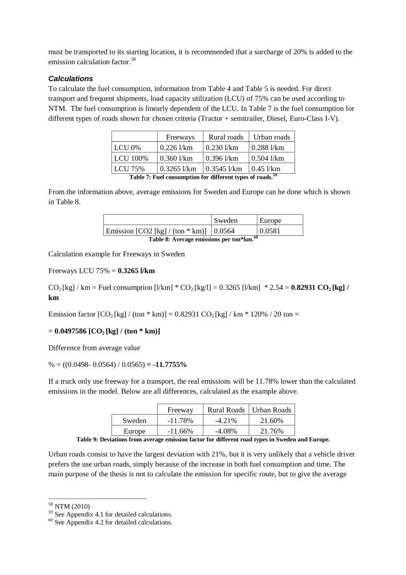
must be transported to its starting location, it is recommended that a surcharge of 20% is added to the

emission calculation factor.58

Calculations

To calculate the fuel consumption, information from Table 4 and Table 5 is needed. For direct

transport and frequent shipments, load capacity utilization (LCU) of 75% can be used according to

NTM. The fuel consumption is linearly dependent of the LCU. In Table 7 is the fuel consumption for

different types of roads shown for chosen criteria (Tractor + semitrailer, Diesel, Euro-Class I-V).

Freeways Rural roads Urban roads

LCU 0% 0.226 l/km 0.230 l/km 0.288 l/km

LCU 100% 0.360 l/km 0.396 l/km 0.504 l/km

LCU 75% 0.3265 l/km 0.3545 l/km 0.45 l/km Table 7: Fuel consumption for different types of roads.

59

From the information above, average emissions for Sweden and Europe can be done which is shown

in Table 8.

Sweden Europe

Emission [CO2 [kg] / (ton * km)] 0.0564 0.0581 Table 8: Average emissions per ton*km.

60

Calculation example for Freeways in Sweden

Freeways LCU 75% = 0.3265 l/km

CO2 [kg] / km = Fuel consumption [l/km] * CO2 [kg/l] = 0.3265 [l/km] * 2.54 = 0.82931 CO2 [kg] /

km

Emission factor [CO2 [kg] / (ton * km)] = 0.82931 CO2 [kg] / km * 120% / 20 ton =

= 0.0497586 [CO2 [kg] / (ton * km)]

Difference from average value

% = ((0.0498- 0.0564) / 0.0565) = -11.7755%

If a truck only use freeway for a transport, the real emissions will be 11.78% lower than the calculated

emissions in the model. Below are all differences, calculated as the example above.

Freeway Rural Roads Urban Roads

Sweden -11.78% -4.21% 21.60%

Europe -11.66% -4.08% 21.76% Table 9: Deviations from average emission factor for different road types in Sweden and Europe.

Urban roads consist to have the largest deviation with 21%, but it is very unlikely that a vehicle driver

prefers the use urban roads, simply because of the increase in both fuel consumption and time. The

main purpose of the thesis is not to calculate the emission for specific route, but to give the average

58 NTM (2010) 59 See Appendix 4.1 for detailed calculations. 60 See Appendix 4.2 for detailed calculations.

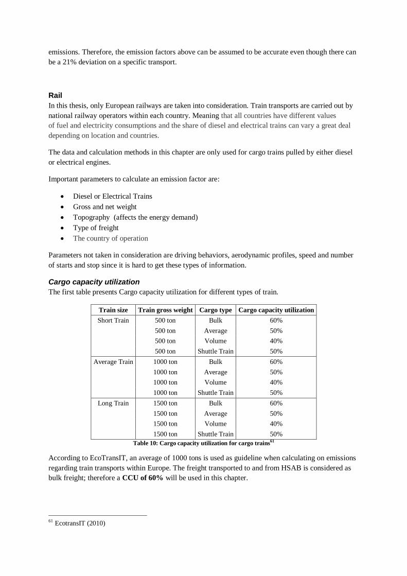
emissions. Therefore, the emission factors above can be assumed to be accurate even though there can

be a 21% deviation on a specific transport.

Rail

In this thesis, only European railways are taken into consideration. Train transports are carried out by

national railway operators within each country. Meaning that all countries have different values

of fuel and electricity consumptions and the share of diesel and electrical trains can vary a great deal

depending on location and countries.

The data and calculation methods in this chapter are only used for cargo trains pulled by either diesel

or electrical engines.

Important parameters to calculate an emission factor are:

Diesel or Electrical Trains

Gross and net weight

Topography (affects the energy demand)

Type of freight

The country of operation

Parameters not taken in consideration are driving behaviors, aerodynamic profiles, speed and number

of starts and stop since it is hard to get these types of information.

Cargo capacity utilization

The first table presents Cargo capacity utilization for different types of train.

Train size Train gross weight Cargo type Cargo capacity utilization

Short Train 500 ton Bulk 60%

500 ton Average 50%

500 ton Volume 40%

500 ton Shuttle Train 50%

Average Train 1000 ton Bulk 60%

1000 ton Average 50%

1000 ton Volume 40%

1000 ton Shuttle Train 50%

Long Train 1500 ton Bulk 60%

1500 ton Average 50%

1500 ton Volume 40%

1500 ton Shuttle Train 50%

Table 10: Cargo capacity utilization for cargo trains61

According to EcoTransIT, an average of 1000 tons is used as guideline when calculating on emissions

regarding train transports within Europe. The freight transported to and from HSAB is considered as

bulk freight; therefore a CCU of 60% will be used in this chapter.

61 EcotransIT (2010)

Topography and electricity/fuel consumption

The topography has a major impact on the electricity and fuel consumption. Therefore, Europe is

divided into three types of topography. These are flat terrain, hilly terrain and mountainous terrain.

Countries considered flat are Denmark, Netherlands and Sweden. Countries consists of mountainous

terrain are Switzerland and Austria. Rest of Europe is hilly terrain.62

In the tables below, the electricity

and fuel consumption for different topographies are shown.

Traction Topography Gross weight range Fuel consumption

Diesel Flat terrain 500-1500 ton 122,46*Wgr-0,5

Diesel Hilly terrain 500-1500 ton 153,07*Wgr-0,5

Diesel Mountainous terrain 500-1500 ton 183,69*Wgr-0,5

Table 12: Fuel consumption for different topographies [g/gross ton * km]

From the two tables above, calculations are made to develop following electrical and fuel

consumptions.63

62 Ibid 63 NTM (2010)

Traction Topography Gross weight range Electricity consumption

Electrical Flat terrain 500-1500 ton 540*Wgr-0,5

Electrical Hilly terrain 500-1500 ton 675*Wgr-0,5

Electrical Mountainous terrain 500-1500 ton 810*Wgr-0,5

Table 11: Electricity consumption for different topographies [Wh/gross ton * km]

Terrain

Train size Train gross weight Cargo type Flat Hilly Mountainous

[kWh/km]

Short Train 500 ton Bulk 12 15 18

500 ton Average 12 15 18

500 ton Volume 12 15 18

500 ton Shuttle Train 12 15 18

Average Train 1000 ton Bulk 17 21 26

1000 ton Average 17 21 26

1000 ton Volume 17 21 26

1000 ton Shuttle Train 17 21 26

Long Train 1500 ton Bulk 21 26 31

1500 ton Average 21 26 31

1500 ton Volume 21 26 31

1500 ton Shuttle Train 21 26 31

Table 13: Electricity consumption different types of trains and topographies [kWh/km]

Terrain

Train size Train gross weight Cargo type Flat Hilly Mountainous

[l/km]

Short Train 500 ton Bulk 3,29 4,11 4,94

500 ton Average 3,29 4,11 4,94

500 ton Volume 3,29 4,11 4,94

500 ton Shuttle Train 3,29 4,11 4,94

Average Train 1000 ton Bulk 4,65 5,82 6,98

1000 ton Average 4,65 5,82 6,98

1000 ton Volume 4,65 5,82 6,98

1000 ton Shuttle Train 4,65 5,82 6,98

Long Train 1500 ton Bulk 5,7 7,13 8,55

1500 ton Average 5,7 7,13 8,55

1500 ton Volume 5,7 7,13 8,55

1500 ton Shuttle Train 5,7 7,13 8,55

Table 14: Fuel consumption different types of trains and topographies [l/km]

Emissions caused by electricity generation

The following table has been adopted from the EcoTransIT project. The table present CO2 emissions

for the electricity supply for railway transports within European countries.

Country CO2 [kg/kWh]

Austria 0,01

Belgium 0,26

Czech Republic 0,71

Denmark 0,48

Finland 0,21

France 0,11

Germany 0,66

Hungary 0,55

Italy 0,49

Luxembourg 0,26

Netherlands 0,43

Norway 0

Poland 0,94

Slovakia 0,18

Slovenia 0,37

Sweden 0

Switzerland 0

EU average 0,41

Table 15: CO2 emissions for regional electric train supplies regarding European countries64

64 EcoTransIT (2010)

The CO2 Total in Diesel can be calculated by multiplying the carbon content in mass-% with the fuel

density and the molecular weight relations given in such that all carbon is transformed into CO2, and

that the small amount of CO, hydrocarbons and particles are neglected (Same as Road).

Weight relations:

The equation to calculate kg CO2 per liter fuel:

And diesel specific:

Calculations

Calculation of emission factors regarding electric and diesel trains:

Example electric train

An electric train in Denmark with the total gross weight of 1000 tons and a load factor stated as 60%.

(Denmark is considered flat)

Electricity consumption = 540*Wgr-0.5

= 540*1000-0.5

= 17.07 [Wh / gross ton * km].

Electricity consumption per net ton = 17.07 / 0.6 = 28.45 [Wh / net ton * km].

There are losses in transmissions which will increase the electricity consumption by ~10% according

to EcoTransIT. The cause of these losses is considered to be resistive, transformation losses and

frequency modulation.

From Table 15, Denmark has an emission factor of 0.48 CO2 kg/kWh regarding railway transports.

Therefore, giving the emission factor

Country CO2 g / net ton km

Austria 0,47

Belgium 10,28

Czech Republic 28,07

Denmark 15,18

Finland 8,30

France 4,35

Germany 26,09

Hungary 21,74

Italy 19,37

Luxembourg 10,28

Netherlands 13,60

Norway 0,00

Poland 37,16

Slovakia 7,12

Slovenia 14,63

Sweden 0,00

Switzerland 0,00

EU average 16,21

Table 16: Emission factor regarding electric trains in European countries

Example diesel train

A diesel train in hilly topography with total gross weight of 1000 tons and a load factor stated as 60%.

Fuel consumption = 153.07 Wgr-0.5

= 153.07 1000 -0.5

= 4.84 [g/gross ton km]

Fuel consumption per net ton

Fuel consumption per net ton in liter

CO2 kg in 1 liter diesel

Therefore, giving the emission factor =

The table below shows the emission factor for different topographies

Topography CO2 g / net ton km

Flat 20,43

Hilly 25,54

Mountainous 30,65

Table 17: Emission factor (Diesel train) for different topographies

In order to keep the simplicity of the model, it is impossible to have an emission factor for every single

country. For the electric train the emission factors varies from 0 to 37 g/net ton*km. Diesel train varies

from 20 to 30 g/net ton*km. The parameter regarding the distribution percentage in total, between the

electric and the diesel trains was not possible to gain during the study. However, 85-90% of the train

transports outside of Sweden in HSAB´s account go through Germany, which has an electricity

emission factor of 26 and is very close to the emission factor for diesel trains in comparison.

The average emission factor for electricity train in Europe except Germany and Sweden is 12.7 CO2 g

/ net ton km. This leads to:

Germany 90% * 26.09 + Rest of Europe 10% * 12.7 = 24.75 CO2 g / net ton km

Therefore, an approximation of 25 CO2 g / ton*km for trains outside Sweden can be made, even if

there are uncertainties if electricity or diesel is used. Sweden is an exception due to the emission

values here is stated as zero (See Table 16) and will have 0 CO2 g / ton*km as emission factor in the

model .

Sea

These sea transport sector can be divided into two different types: ferries and container ships. The

ferries are used in short distance transports and are combined cargo and passenger ships. The container

ships are used in long distances and contain only cargo loaded in containers.

The ferries used in this case are so called RoRo (roll on – roll off) and RoPax (limited passenger

capacity) ferries, where cars and trucks drive onto the ferry via an off-shore ramp.

Container ships can be divided into two different types of ships, feeder ships and larger container ships

used for intercontinental cargo transport which will be referred as container ships further on.

Feeder ships are smaller container ships used to allocate the cargo to feeder harbors where the cargo

gets loaded on container ships. This is done to streamline the transport chain, because it´s more

efficient for the feeder ships to allocate small amount cargo from minor harbors instead of having the

large container ships to run on shorter routes. In HSAB´s case, the cargo transports made by feeder

and container ships have two different routes. Either the cargo leaves Höganäs with a truck to

Gothenburg harbor. In Gothenburg harbor, the cargo is loaded on feeder ships and transported to a

feeder harbor in northern Europe. The other route is from Höganäs to Helsingborg harbor where the

cargo is loaded on feeder ships and transported to a feeder harbor. From the feeder harbor the

container ships transport the cargo to Asia, South America and North America.

However, to keep the simplicity of the model, the feeder ships have been excluded in the model. The

main reason for this is the uncertainty of which feeder harbor that is used during transportations. There

are no fixed routes or harbors used by the shipping companies; instead the cargo is re-routed

throughout a series of larger feeder harbors such as Bremerhaven, Antwerp or Zeebrugge. The chosen

port depends mainly on the cost and time efficiency at that certain point of time for each of the larger

container ships. This making it almost impossible to keep track of which route that was taken per

transport.65

To be able to perform calculations for the emission factors a data collection has to be done. There are

many different types of ferries, fuel types and engines which make it difficult to estimate the emission

factor if there are no chart of the distribution for each type of ferry, fuel and engine in HSABs case.

Even if the emission factor is possible to calculate for some type of ferries, the uncertainty is too high

to establish the value as accurate enough.

EcoTransIT has a calculator on their website where the user is able to calculate the emissions for sea

transport. This tool has been developed from a very large database collected from transport companies

with the exact volumes, routes via GPS and fuel consumption. This database is not public and there

are no numbers presented by EcoTransIT except the calculation tool.

Therefore, it was decided to use the same emission factors as EcoTransIT use in their calculator. For

container ships the values 10 g CO2/ ton * km are used and 47 g CO2/ ton * km for ferries.

65 Schönhult, Carl-Johan 2011-04-10

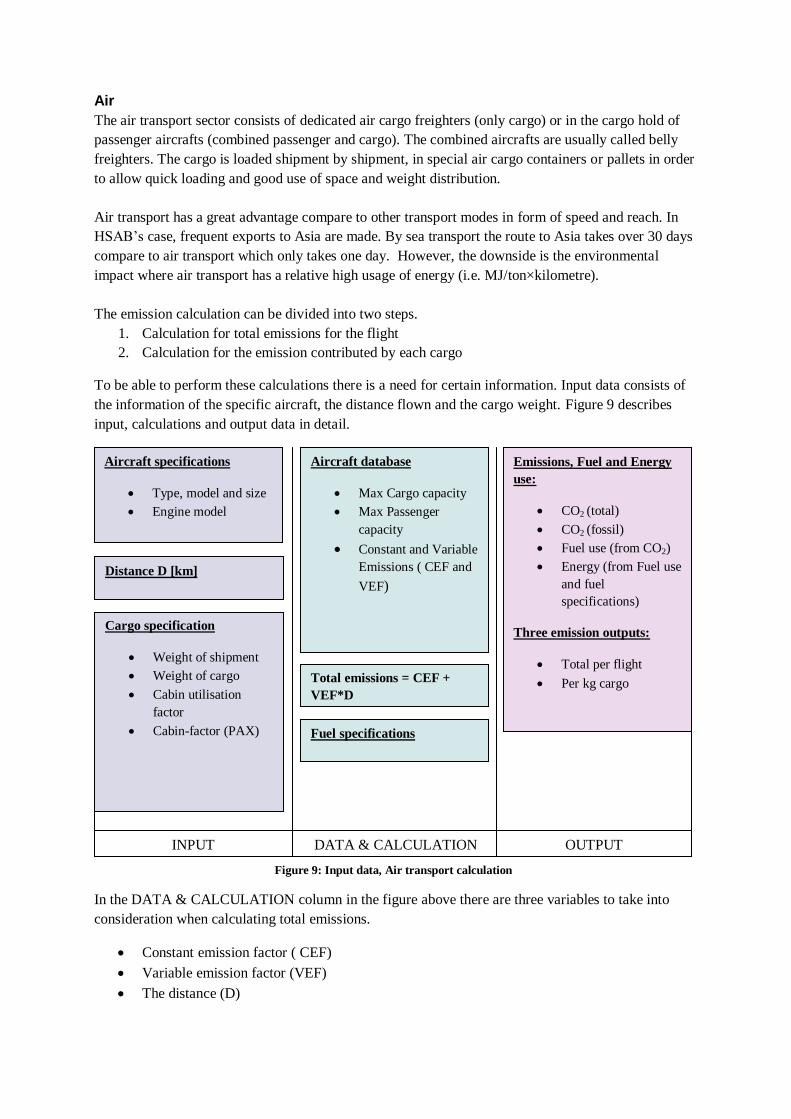
Air

The air transport sector consists of dedicated air cargo freighters (only cargo) or in the cargo hold of

passenger aircrafts (combined passenger and cargo). The combined aircrafts are usually called belly

freighters. The cargo is loaded shipment by shipment, in special air cargo containers or pallets in order

to allow quick loading and good use of space and weight distribution.

Air transport has a great advantage compare to other transport modes in form of speed and reach. In

HSAB’s case, frequent exports to Asia are made. By sea transport the route to Asia takes over 30 days

compare to air transport which only takes one day. However, the downside is the environmental

impact where air transport has a relative high usage of energy (i.e. MJ/ton×kilometre).

The emission calculation can be divided into two steps.

1. Calculation for total emissions for the flight

2. Calculation for the emission contributed by each cargo

To be able to perform these calculations there is a need for certain information. Input data consists of

the information of the specific aircraft, the distance flown and the cargo weight. Figure 9 describes

input, calculations and output data in detail.

In the DATA & CALCULATION column in the figure above there are three variables to take into

consideration when calculating total emissions.

Constant emission factor ( CEF)

Variable emission factor (VEF)

The distance (D)

Aircraft specifications

Type, model and size

Engine model

Distance D [km]

Cargo specification

Weight of shipment

Weight of cargo

Cabin utilisation

factor

Cabin-factor (PAX)

Aircraft database

Max Cargo capacity

Max Passenger

capacity

Constant and Variable

Emissions ( CEF and

VEF)

Total emissions = CEF +

VEF*D

Fuel specifications

Emissions, Fuel and Energy

use:

CO2 (total)

CO2 (fossil)

Fuel use (from CO2)

Energy (from Fuel use

and fuel

specifications)

Three emission outputs:

Total per flight

Per kg cargo

INPUT DATA & CALCULATION OUTPUT

Figure 9: Input data, Air transport calculation

CEF represents taxi out, start, climb to cruise, descend from cruise, landing and taxi in, i.e. every

factor that does not get affected by distance.

VEF is the factor which is multiplied with the distance to calculate the fuel consummation in the air.

The calculations for the distances will be explained later in this section.

Figure 10 explains the principals of the Total emissions = CEF + VEF*D formula.

Figure 10: Emission-Distance calculation66

HSAB use airfreights when short term deliveries are requested. None of the airfreight transports are

originally scheduled and are only used on customer demand or when unforeseen complications occur

during the production or planning process of an order that severely affects lead-times. The airfreight

transports consists of mainly long distance flights to the regions Asia, USA and the Oceanic’s

One of the main criteria for the emission model is that it has to be easy filling in the variables to be

able to calculate emissions. Therefore, a general emission factor was developed and applied to

all transports within the air sector.

The input data used are taken from the logistic company Airlog which stands for approximately 94%

of the air transports that are conducted by HSAB. Airlog uses mainly four different aircrafts during

transportation. Airbus 330-300 and Airbus 340-300 which are used at routes trafficked by SAS and

Finnair. Airbus 340-400 and Boeing 787 are used by Korean, Air China and China Airline. All of

these aircrafts are so called belly freighters.

NTM have data tables for different aircrafts, but only for Airbus 330-300 and Airbus 340-300 of the

four different aircrafts used by Airlog. In the table at NTM Airbus 340-300 are equipped with the old

engine CFM56-5C3, but in the reality they have been replaced with the more effective CFM56-5C4

engine. Airlog also gave the information of an average pay load factor at 90% for their flights.67

The table shown below is data from NTM for Airbus 330-300 and Airbus 340-300 with different

payload factors.

66 NTM (2010) 67 Rosenkvist, Johan. Managing director, Airlog 2011-03-25

Aircraft

Max

Payload

Load

Max

Pax

Load

Cabin

Factor

Max

Cargo

Load

Cargo

Factor

Max

Distance CO2 CO2

CEF VEF

[kg] [kg] [%] [kg] [%] [km] [kg] [kg/km]

A340-300 47320 23933 65 13000 50 14998 8987 23,11

A340-300 47320 23933 90 13000 50 14846 9401 23,32

A340-300 47320 23933 65 13000 100 14830 9439 23,35

A340-300 47320 23933 90 13000 100 14167 9850 23,47

A330-300 46695 30391 65 20000 50 9237 8059 23,67

A330-300 46695 30391 90 20000 50 8193 8701 23,68

A330-300 46695 30391 65 20000 100 7863 8905 23,68

A330-300 46695 30391 90 20000 100 6819 9553 23,7

Table 18: Data gathered concerning Airbus series 330-300 and 340-30068

In order to check if there is any linear connection between Pax Load + Cargo Load and CEF and VEF

a calculation was made. CEF and VEF were divided by the total load in order to get [kg emissions /

kg load] and [kg emissions / (kg load * km)]. The result for each payload factor is presented in Table

19 below.

Total Load kg CEF [kg emissions / kg load] VEF [kg emissions / (kg load * km)]

A340-300 22056 0,41 0,00105

28040 0,34 0,00083

28556 0,33 0,00082

34540 0,29 0,00068

A330-300 29754 0,27 0,00080

37352 0,23 0,00063

39754 0,22 0,00060

47352 0,20 0,00050

Table 19: CEF & VEF specifics for A330-300 and A340-30069

The table shows there is no linear connection between Total Load and CEF or VEF. Therefore, an

assumption had to be made. Cargo Factor is said to be 90%, but the Cabin Factor is unknown. A

reasonable assumption would be to pick alternative three for both aircraft. The Cargo Factor is

somewhat lower (90% against 100% in the table), while Cabin Factor can be assumed to be higher

than the 65% stated in the table.

For Airbus 340-300 the values for CEF and VEF will be 0.33 [kg emissions / kg load] respectively

0.00082 [kg emissions / (kg load * km)] and for Airbus 330-300 the values will be 0.22 [kg emissions

/ kg load] respective 0.00060 [kg emissions / (kg load * km)]. In order to get a general emission factor,

an average of the values for the two aircrafts will be used in following calculations. The average CEF

is 0.28 [kg emissions / kg load] and the average VEF is 0.00071 [kg emissions / (kg load * km)].

Next step regards distance calculation. As said before, one of the main criteria for the emission model

is that it has to be easy filling in the variables to be able to calculate the emissions, therefore it is not

68 NTM (2010) 69 Ibid

possible to get detailed information for each flight i.e. Airlog used ten different airports to send cargo

from Europe in 2010 but in the model only an average distance is used.

To develop an average distance only the three most trafficked airports were used. The three airports

were Copenhagen, Frankfurt and Helsinki which were used by 77% of the flights. The distance

between the three airports and the final destinations were calculated on the website

http://www.indianindustry.com and then divided by three to get an average distance. Following results

were shown.

Country Volume [Ton] Average Distance [km]

Adelaide 0,40 15429

Melbourne 3,00 16300

Sao Paulo 53,64 9842

Other than AirLog 4,35 9842

Shanghai 35,67 7783

Other than AirLog 0,03 7783

Mumbai 15,07 6808

Other than AirLog 8,00 6808

Tehran 0,50 6815

Osaka 20,07 7966

Tokyo 81,80 8298

Busan 8,01 7644

Incheoni(Seoul) 8,50 7382

Other than AirLog 7,00 7382

Mexico City 0,03 9574

Kuala Lumpur 1,00 11625

Bangkok 9,85 8284

Istanbul 0,60 2145

Taipei 1,00 8347

Orlando 0,04 7643

Campbellsburg(Louisville) 2,00 8794

New York 8,25 6203

Hollsopple(Pittsburgh) 36,22 6711

Quebec (DHL) 6,00 6637

Delhi (Grencarrier) 0,50 7562

Randburg (Other) 0,01 8774

Guelph (Other) 5,00 6822

TOTAL 316,54

Table 20: Average calculated distances regarding HSAB air transports.

To obtain the average distance per flight all distances are multiplied with the specific volumes and

divided by total volume (316.54 tons). The average distance for all flights for HSAB is 8124 km.

The airline and logistic companies always strive to have as few stopovers as possible, therefore is the

CEF part only multiplied by 1, i.e. no regards to stopovers are made in the calculation.

The emissions for a flight are as follows:

With the numbers from above, the values in HSAB’s case is

This gives 0.0007408 emission C02 [kg / kg load * km]

Rewritten to the unit [g / ton load * km], the specific emission factor for the flights made by HSAB

will be 740.8 C02 [g / ton load * km].

To be sure this emission factor is accurate, calculations were made to see that the deviations from the

Total emission = CEF + VEF * distance formula are not too large.

Total Volume CEF VEF

A340-300 28556 0,33 0,00082

A330-300 39 754,15 0,22400177 0,000596

Table 21: Values for CEF and VEF from relevant cases

Worst case scenarios are when the routes are extremely short and extremely long.

Calculations for shortest route, 2145 km, using a A340-300 aircraft with

formula.

Calculations using our emission factor of be 740.8 C02 [g / ton load * km]

kg C02

Using kg in the first calculation, the second result has to be divided by 1 000 000 to get correct unit.

Total emission using our emission factor is 1.589.

The difference in percent is 24% less emissions if using the emission factor. The table below shows

the numbers for shortest respectively longest flights for both aircrafts.

Distance Emission (CEF and VEF) Emission (using emission factor) Difference %

A340-300 2145 2,08 1,59 -24

A330-300 2145 1,50 1,59 6

A340-300 16300 13,66 12,08 -12

A330-300 16300 9,93 12,08 22

Table 22: Differences in using formulas shortest and longest flights

Figure 11: The figure shows the volumes and how the different types of aircraft differ from the average emission factor depending of the distance.

Figure 11 shows the deviations from the average emissions factor depending of the distance. The two

lines shows the real emissions for the two different aircrafts calculated with the

formula. Aircraft A340-300 has higher emissions than the average

emission factor and the A330-300 has lower emissions. To get a correct average emission factor, the

distance from the two lines to the 0.00% line should be equal.

As seen in Figure 11 and in Table 22, for 2000 km flights with the A340-300 aircraft the real

emissions are approximately 25% higher than the calculated emissions. For 16000 km flights with the

A330-300 aircraft the real emissions are approximately 20% lower than the calculated emissions.

However, the Figure 11 also shows the volumes transported by distances. As seen in the figure, a large

amount of the total cargo is between 6000 km and 10000 km where the two aircrafts lines are at the

same distance from the calculated emissions line. This gives the average emissions factor can be

assumed to be correct if both types of aircrafts are used equal number of times, but for a specific flight

the calculated emissions in the model can be 25% lower than the real emission.

If only one of the two different types of aircrafts is used, the difference between the emission factor

calculations and real emissions can be approximately -15% to +15% for all flights in total.

The emission factor used in the model will therefore be 740.8 C02 [g / ton load * km].

The Emission Model

The description and interface of the developed model are shown in this chapter. The sentence of this

section is to show the reader some insight and knowledge upon the model structure and set-up.

The Model

This part of the thesis contains a more detailed explanation of the model done in Microsoft Excel. The

model can be divided into three parts, overview, input data and the part that contain all customer

information sorted by each region.

Overview sheet

The first sheet is the Overview sheet which shows global distribution emissions values, inbound

logistics emissions values, emissions for each mode of transport, emissions per volume transported for

each region, emissions shown as CO2/Ton-kilometer and emissions for inbound freight transports.

Input data

In the Input data sheet the user is able to change input values for the model. The most important

feature is the emission factor table. The values for each emission factor have been presented in

previous chapters, but can easily be changed for future changes such as improved transportation

methods and more efficient motor characteristics.

Note: If the emission factor values are changed, all the values in the model are automatically aligned

as such.

The other feature in the Input data sheet is the sea distance calculator. Since HSAB is transporting

large volumes of shipments to Asia, it is of highest importance that distances between these two

continents is accurate. These distances are basically divided into two different routes that one could

take, either through the Suez Channel or the around the African continent. The route that is

chosen depends upon a variety of different factors. These can include parameters such as transport

fees when sailing through the Suez Channel, oil prices, pirate threats outside Africa's east coast and

customer delivery demands.

The top right table, the user can divide in percentage how much of the annually shipments goes

through the different routes. When changing these values, the average distances for all transports from

Europe to Asia are automatically changed.

The user is also able to change the add-on percentage of the different transport routes since taken

routes rarely are direct from starting origin to final destination. These values are explained and

calculated in the chapter regarding emission factors.

Region sheets

There are eleven regional sheets, a sheet for air export and one for all incoming freight shipments. The

air export has its own sheet because the utilization of air transports is never originally scheduled and

differ variously from year to year, both regarding in volumes and/or destination wise.

In every region sheet there are columns with customer names, volumes, sub-destinations and final

destinations. The destination columns contain two to four columns depending of the need to have

different transport modes for the same shipment. See Figure 12 for example.

Germany

Sea

Italy

Road/rail

Sweden

Road/Rail

Figure 12: illustration of route between Sweden and Italy

In every region sheet there is a small compilation table under the main table. The main reason for the

compilation is to simplify the creation of the Overview sheet.

Air Sheet

The Air Sheet contains all air transports done during 2010 in HSAB´s accounting. The Air sheet only

contains one column for destinations, which makes it a bit smaller than the regional sheets. The

emission factors and the distances have been explained in other chapters. Where it is stated “Other

than AirLog”, another supplier is utilized. Note that AirLog are used for approximately 95% of the

utilized air shipments.

Incoming Transport Sheet

The last sheet contains all incoming transports where the majority of shipments are distributed to

Höganäs. The sheet has the same build up as the regional sheets except destination origin is at the

supplier’s address location and HSAB is stated as the final destination.

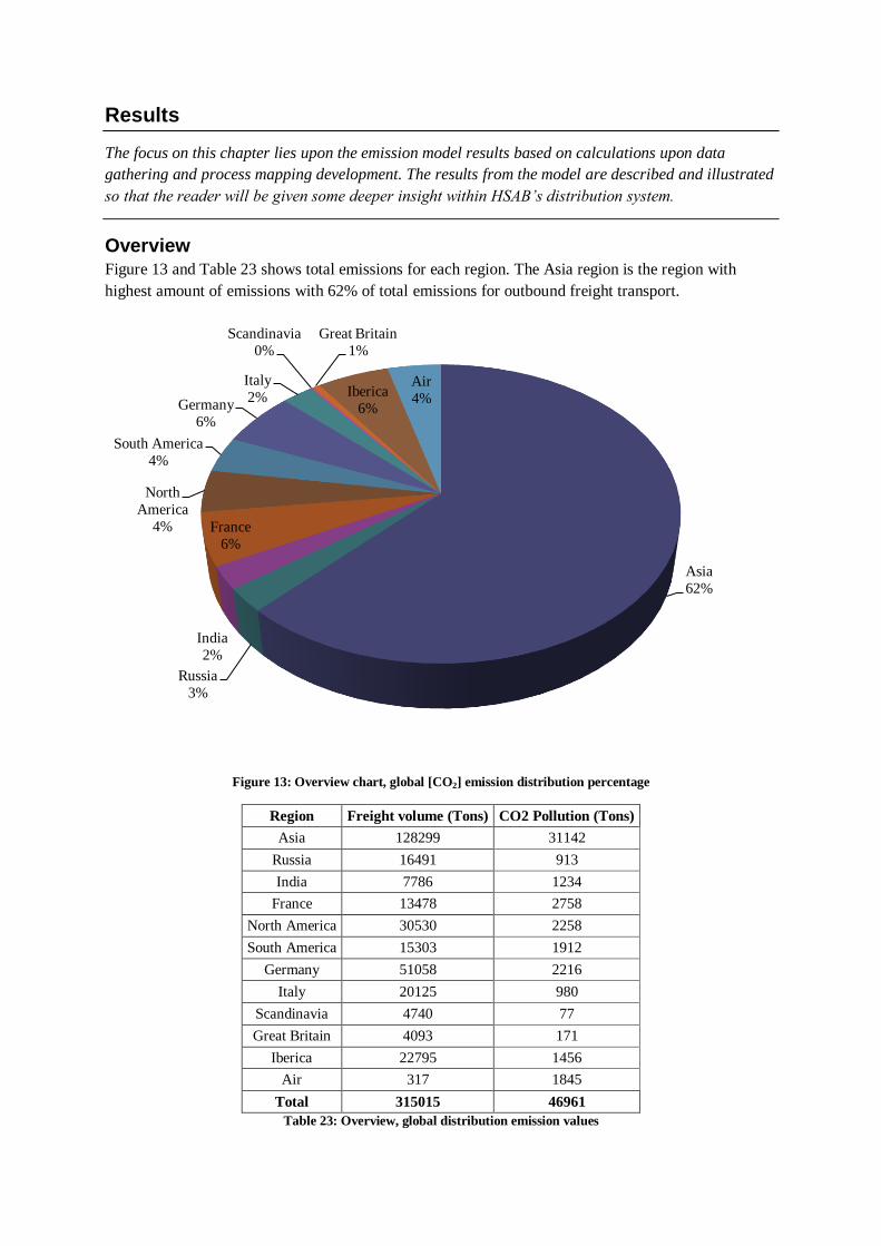
Results

The focus on this chapter lies upon the emission model results based on calculations upon data

gathering and process mapping development. The results from the model are described and illustrated

so that the reader will be given some deeper insight within HSAB’s distribution system.

Overview Figure 13 and Table 23 shows total emissions for each region. The Asia region is the region with

highest amount of emissions with 62% of total emissions for outbound freight transport.

Figure 13: Overview chart, global [CO2] emission distribution percentage

Region Freight volume (Tons) CO2 Pollution (Tons)

Asia 128299 31142

Russia 16491 913

India 7786 1234

France 13478 2758

North America 30530 2258

South America 15303 1912

Germany 51058 2216

Italy 20125 980

Scandinavia 4740 77

Great Britain 4093 171

Iberica 22795 1456

Air 317 1845

Total 315015 46961

Table 23: Overview, global distribution emission values

Asia

62%

Russia

3%

India

2%

France

6%

North

America

4%

South America

4%

Germany

6%

Italy

2%

Scandinavia

0%

Great Britain

1%

Iberica

6%

Air

4%

Figure 14 and Table 24 shows freight volumes for each region regarding inbound freight transports.

Sweden has the largest amount of freight volume, but Mauritania has the largest amount of emissions

with 7551 tons CO2. These two regions have the largest impact on Höganäs AB total emissions for

inbound freight transports.

Figure 14: Overview chart, global [CO2] emission inbound logistics percentage

Region/Country Freight Volume (Tons) CO2 Pollution (Tons)

Austria 220 7

Belgium 67 3

Brazil 69 9

Switzerland 392 28

Chile 339 50

China 2 0

Germany 16376 554

Denmark 1318 15

France 301 5

Great Britain 35549 911

India 1315 199

Italy 1015 44

Mauritania 84001 7551

Netherlands 4 0

Norway 583 39

Sweden 343405 7190

USA 3949 288

South Africa 375 58

Total 489280 16952

Table 24: Overview, inbound logistics emission values

Other

1%

Germany

2% Great Britain

7% India

1%

Mauritania

39%

Sweden

49%

USA

1%

Figure 15 and Table 25 illustrates the total emission value for each mode of transport. Sea

Intercontinental shows the largest emission value, which can be explained by the large volume

quantities of goods that is transported to Asia.

Figure 15: Emission percentage per transport mode regarding distribution

Type Emissions(ton)

Road Sweden 1 261

Road Europe 3 773

Train 801

Train Sweden 0

Aircraft Intercontinental 1 845

Short distance sea 3 389

Sea Intercontinental 32 834 Table 25: Total emissions for each mode of transport.

Road Sweden

3%

Road Europe

8%

Train

2%

Train Sweden

0% Aircraft

Intercontinental

4%

Short distance sea

8%

Sea Intercontinental

75%

Figure 16 and Table 26 shows the emission kg CO2 per volume (ton) transported for each region,

which can be translated to the cost in emission per transport to each region.

Figure 16: Emission CO2 per volume transported for each region.

Region/Type CO2 (kg)/Volume(ton)

Asia 243

Russia 55

India 158

France 205

North America 74

South America 125

Germany 43

Italy 49

Scandinavia 16

Great Britain 42

Iberica 64

Air 5830

Table 26: Distribution emissions for each assigned cargo destination [CO2 value per ton]

Table 27 and Figure 17 shows CO2 /Ton-kilometer, in other words, how effective it is to transport

goods to the different regions from an emission perspective. The regions with lowest emission per

volume-kilometer are the regions where Sea Intercontinental is the main mode of transport.

Figure 17: Emissions shown as CO2 /Ton-kilometer.

Region/Type Emission(kg)/Volume(ton) * km

Asia 10

Russia 19

India 10

France 39

North America 10

South America 10

Germany 41

Italy 32

Scandinavia 56

Great Britain 31

Iberica 29

Table 27: Distribution emissions shown as CO2 /Ton-kilometer

Figure 15Figure 18 and Table 28 illustrates the total emission value for each mode of transport

regarding inbound freight transports.

Figure 18: Emission percentage per transport mode regarding inbound freight transports

Type Emissions(ton)

Road Sweden 3 054

Road Europe 582

Train 39

Train Sweden 0

Aircraft Intercontinental 0

Short distance sea 19 295

Sea Intercontinental 5 315 Table 28: Total emissions for each mode of transport.

Road Sweden

11%

Road Europe

2%

Train

0%

Train

Sweden

0%

Aircraft

Intercontinental

0%

Short distance sea

68%

Sea Intercontinental

19%

Conclusion and discussion

The main findings upon reviewing the presented results are stated in this final chapter of the study.

Furthermore the chapter will discuss model recommendations, limitations and possibilities for further

research advancement. The chapter is initiated by a brief summary of the thesis study

The purpose of this thesis was to present a model that can be applied as an everyday tool that

calculates the total emissions caused by freight transport throughout the Höganäs Group. A partial

objective was also to give recommendations of possible means to reduce CO2 emissions.

From the theoretical framework gathered by the initiation of this study, a model was brought forward

with the purpose of identifying a company’s carbon dioxide emissions during in\- outbound logistics.

The created calculation tool is a result of adapted process mapping methodology, powered by data

gained through interviews and intern ERP-systems. The results from the calculation tool provide

insight of freight transport within HSAB and shows areas of potential for future environmental

opportunities.

The model

The model was created in the computer software Microsoft Excel. As regularly used software, this

fulfills the requirement that the model should be easy to use.

In order to maintain simplicity of the model, the information and input values collected by the user are

limited to specific sections of the model to prevent the possibilities for result errors. Volumes and

distance values are static parameters that have to be manually corrected by user when modifications

are made in distribution systems in order to reflect accurate results.

The model is served primarily as a tool to calculate overall emission values throughout the company’s

transportation network. Other parameters affecting emission values are types of transports used and its

specific engine class and characteristics. An example is that there for instance are two different

aircrafts in this thesis with two different emission values. In order to maintain the easy handling

operations for end-user, an average emission factor for these has been calculated. This can lead to

deviations in real-life affiliation depending on which aircraft is used. The deviations in this case can be

as high as 25%, but it is only on rare occasions. Same values for road transports are up to 21%. Due to

these deviations, the model therefore should not be utilized for singular transport purposes. To obtain

more information regarding the calculated emission values for each mode of transport, please refer to

the chapter regarding “Project calculation approach”.

When calculations in the model are made, the user obtains illustrative information regarding each sales

region. Information in terms of total emission values, emissions per volume, emissions per volume-

distance and emission for each mode of transport are shown in directly within the model. To read more

about the model and how to edit and/or add to the customer base, please refer to Appendix 3 section of

this report.

Main findings

After reviewing the result section of this study, it can be concluded that the total emission value

regarding freight distribution at HSAB lies around 45 000 tons of carbon dioxide. Note that the Asia

region stands for nearly two-thirds of the total emission count. The high emission value released from

Asia region can be explained by the long distances from Sweden to Asia and the huge amount of cargo

the company sends to this region on a yearly basis. In 2010 HSAB exported more than 315 000 tons of

material where 128 000 of these were exported to Asia.

To be able to see where improvements can be done to reduce the CO2 emissions, a more detailed

insight than the traditional overview chart is needed. Table 26 in previous chapter shows as an

example how much emission every ton cargo causes to a specific destination. Asia consists as the

largest contributor which is no surprise since distances to Asia are the longest.

Table 27 displays carbon dioxide values as emission (kg)/volume (ton) * km. This shows the emission

efficiency for transportation to a certain region. A low emission value equals the utilization of

transport modes with low CO2 emission factors. Looking at this table shows that the region with the

highest emission count is Scandinavia. This can be explained by the high utilization of truck and

trailer within this region. Regions where sea transport is the main mode of transportation have the

lowest emission values, i.e. Asia, India, South America and North America.

The total emission value for incoming goods are only a third in comparison to emission values

regarding exported goods even though HSAB imports 150 000 tons more than they export. This is a

result of the large amount of domestic imported freight with short transport distances.

Improvements Due to the fact that HSAB has outsourced transport activities to various freight forwarders, it is

difficult for the company to apply major changes in the aspect of transportation logistics. The most

obvious statement is to change mode of transport to a more emission efficient type when it is possible.

This has proven to be difficult due to specific customer demands regarding when cargo is to be

delivered in a certain way and time and has become obstacles in search of more eco-friendly solutions.

Nevertheless, these are important variables to take into consideration, especially when reflecting upon

possibilities of changing way of transports. Therefore it is suggested that mutual dialogues are made

between the different actors in the supply chain to reach a consensus effort of providing a more

environmental effective transport solution where each part is equally committed in order to reach the

common goal of reducing its carbon footprint.

A related subject though that is gained throughout the investigations made in this report is the

importance of production planning. This insures that each shipment cargo is planned at full capacity in

terms of volume when possible and that demanded delivery times are met so that contingency plans

including air transported cargo are avoided at all costs due to its high environmental impact.

During the study in coherence with freight forwarders, investigations were made regarding whether if

possibilities of enabling trailers as carriers for two containers simultaneously could be an option of

reducing number of transports and therefore reducing emission levels. But these investigations were

denied by the national road administration due to the consequence of road abrasions. Nevertheless,

should this matter be taken into matter and further investigated when future developments and

technologies are considered.

Recommendation for further studies

As stated above, the region that represents the largest source of carbon dioxide emissions is Asia. And

therefore it is concluded that this region should be prioritized in any discussions around improvement

possibilities regarding reductions in greenhouse gas emissions.

Other findings and recommendations from this study will primarily serve as a basis for future

guidelines. The new insights can, in order of the authors’ recommendations, be used in areas such as:

Environmental analysis of freight forwarder selections during nomination periods

Baseline during evaluation of new logistical solutions

Underlying documentation during internal /external emission evaluations

For use in promotional purposes

Note that in order to keep the models useful purposes its database needs to be updated regularly to

keep producing real life accurate emission values.

References

Published

ARTEMIS, 2008. “ARTEMIS: Assessment and reliability of transport emission models and inventory

systems. Final report”. TRL Limited

Arbnor, Ingeman & Bjerke, Björn (1997) Methodology for Creating Business Knowledge. SAGE

Publications

Beamon, B (1999) Designing the Green Supply Chain, Logistics Information Management, Vol 12, Iss

4.

Björklund, Maria & Paulsson, Ulf (2003) Seminarieboken. Studentlitteratur, Lund

Blinge, Magnus (2005) ”Cost Effective Measures to Reduce CO2 Emissions in the Air Freight Sector”

Transport Research Institute, Gothenburg

Browne, M. Cullinane, S. McKinnon, A. Whiteing, A. (2010) “Green Logistics: Improving the

environmental sustainability of logistics”, the chartered institute of Logistics and transport (UK)

Bryman A. (1984). The Debate about Quantitative and Qualitative Research: A Question of Method

or Epistemology? The British Journal of Sociology

Carbon Trust (2007) “Carbon Footprinting: An introduction for organizations”, The Carbon Trust,

London

EcoTransIT (2010) “EcoTransIT: Ecological Transport Information Tool. Environmental

Methodology and Data” EcotransIT, 2010

European Commission (2006) “An EU Strategy for Biofuels”

Eriksson L, Wiedersheim-Paul F (1997) ”Att Utreda Forska och Rapportera”, Liber Ekonomi,

Malmö

Holmen, BA and Niemeier, DA (2003) Handbook of Transport and the Environment, Elsevier, Oxford

Höganäs Sverige AB (2009) Management responsibility manifesto. HSAB, Höganäs

Insight (2011) Höganäs newsletter, 1st edition

Kahn Ribeiro, S., S. Kobayashi, M. Beuthe, J. Gasca, D. Greene, D. S. Lee, Y. Muromachi, P.J.

Newton, S. Plotkin, D. Sperling, R. Wit, P.J. Zhou. (2007) “Transport and its infrastructure. In

Climate Change” Cambridge University, Cambridge

Lumsden, Kenth. (2006) ”Logistikens Grunder.” Studentlitteratur, Lund

McKinnon, A (1994) Logistics and the environment. EUROLOG, Brussels

NTM Air (2010) “Environmental data for international cargo and passenger air transport” NTM,

2010

NTM Rail (2010) “Environmental data for international cargo transport – rail transport” NTM, 2010

NTM Road (2010) “Environmental data for international cargo transport – road transport” NTM,

2010

NTM Sea (2010) “Environmental data for international cargo transport – sea transport” NTM,

2010

Stevens, G (1989) Integrating the supply chain: International Journal of Physical Distribution and

Materials Management, Vol 19, Iss 8.

UNFCCC (1998) “Kyoto Protocol to the United Nations Framework Convention on Climate

Change”. United Nations Framework Convention on Climate Change

Websites Eniro <www.eniro.se> 2011

E-ships.net <www.E-ships.net> 2011

HSAB Intranet 2011-06-29

Indian Industry <www.indianindustry.com/travel-tools> 2011

Map24 <www.map24.com> 2011

National Audit Office UK <www.nao.org.uk> 2011-06-06

Professional Traffic Sweden <www.Yrkestrafiken.se> 2011-06-06

Searates <www.searates.com> 2011

Swedish Environmental Protection Agency <www.naturvardsverket.se> 2011-03-04

Swedish Petroleum Institute <www.spi.se> 2011-06-06

United Nations <www.un.org> 2011-03-04

United Nations Environment Programme <www.unep.org> 2011-05-18

Personal communications

Andersson, Mikael (2011) Head of department, Sea & container shipments, GDL

Kielerzstajn, Torsten (2011) Freight Manager, HSAB Logistics divison

Schönhult, Carl-Johan (2011) Freight Coordinator, HSAB Logistics division

Rosenkvist, Johan (2011) Managing director, Airlog

Appendixes

Appendix 1 – General objective target & action plans corresponding to

Management responsibilities, Höganäs AB

Area Objective Indicator (example)

Natural resources Reduce the specific

consumption of raw materials

Tons used/produced

Energy Reduce the specific use of

energy

kWh/ton product

Emissions to air Reduce the emissions of dust,

metals and gases from

production

Specific emissions

[Tons emission/ton produced]

and where required for local

impact reasons, also emissions per year [tons/year]

Emissions to water recipients Reduce the emissions of metals

from production

Specific emissions

[Gram metal/ton produced] and where required for local

impact reasons also emissions

per year [kg/year]

Waste Reduce the specific generation of waste

Specific waste production [tons waste/ton produced]

Industrial noise With margin, comply with local

legislation or site conditions for

emission of noise

dB(A) compared to condition

Environmental risks Work systematically to reduce

environmental risks

Products and processes At product and process development,

concern is taken to the

environmental aspects

Appendix 2 – Questionnaire used during email survey with Freight

Forwarders

Hi,

We are students at LTH that as our master thesis is conduction a study at Höganäs AB were we are

mapping in and outbound transport network in order to calculate their total carbon dioxide emission

from these activities.

We are on progress of mapping the transport network but we are at the point where we need your help

to complete the process. We would be grateful if you could spare us a couple of minutes of your time

to answer the following questions.

Question1: To which destinations are transports made in behalf of Höganäs AB?

Question2: Which routes are taken during these transports?

Question3: Which types of transport modes are used during these routes (preferably also engine class

of transport mode if that type of information is available)?

Question4: If different transport modes are used, please state where these switches are made.

We are utterly grateful for your time!

Best regards

Masoud Zanganeh & Magnus Persson

Appendix 3 – Instruction manual for model

This appendix gives a more detailed description of the model and a manual to make it easier to apply

changes.

The first sheet is called “Overview”. This sheet shows the results for all calculations in the model.

There is no need to do anything in this sheet since all changes in the model will automatically be

updated.

Next sheet is “Input data”. In this sheet the user is able to make some changes. In columns A-F sea

distances is presented. When wanting to add a new harbour, the user has to insert the new harbour in

the table manually. It is important when inserting a new harbour to insert a new row from column A-F

and somewhere between the first row and the last row. See Figure below. Note, do not insert after the

last row!

In the upper right corner the user is able to changes the route. Depending on oil prices, delivery time

and risk of pirates outside the east coast of Africa, the transport companies can either go through the

Suez channel or the whole way around the bay of Africa. Simply change the value in cell right to

“Percentage Suez Channel” marked with a red background and the percentage of Good Hope will

automatically be changed as well.

The last table in the sheet is the emission factors. The current emissions factors have been presented in

the thesis, but if the user wants other values is it just to change the values in the cells and the whole

model will be updated. If the name to the left is changed, do not forget to change the name in the list in

all region sheets.

The next eleven sheets are the regional sheet. Every region has its own sheet with customer id,

volumes, distances and emission variables. If a new customer is to be inserted, the procedure is same

as for new harbors. Simple find the right country, the insert the new row somewhere between the first

and last customer for the chosen country. Fill in the cells and the model is automatically updated.

Next sheet where changes can be applied is the sheet marked “Air”. To insert a new airport, simply

follow the same procedures as for harbors and new customers in the region sheet. The last sheet is the

sheet for incoming freight. Same procedure follows for this one as well, only difference is instead of

starting origin, HSAB is stated as final destination.

Appendix 4 – Calculations

4.1 - Fuel consumption for different types of roads

Freeways

LCU 0% = 0.226 l/km

LCU 100% = 0.360 l/km

LCU 75% = (LCU 100% - LCU 0%) * 0, 75 + LCU 0% = (0.360 -0.226) * 0.75 + 0.226 = 0.3265 l/km

LCU 75% = 0.3265 l/km

Rural Roads

LCU 0% = 0.230 l/km

LCU 100% = 0.396 l/km

LCU 75% = (LCU 100% - LCU 0%) * 0, 75 + LCU 0% = (0.396 – 0.230) * 0.75 + 0.230 = 0.3545

l/km

LCU 75% = 0.3545 l/km

Urban Roads

LCU 0% = 0.288 l/km

LCU 100% = 0.504 l/km

LCU 75% = (LCU 100% - LCU 0%) * 0.75 + LCU 0% = (0.504 – 0.288) * 0.75 + 0.288 = 0.45 l/km

LCU 75% = 0.45 l/km

4.2 - Average emissions per ton*km

With the distribution of roads in Sweden in Table 5, the average fuel consumption is

Average fuel consumption = 0, 3265 l/km [Freeways LCU 75%] * 21% + 0.3545 l/km [Rural Roads

LCU 75%] * 56.7% + 0.45 l/km [Urban Roads LCU 75%] * 22.3% =

= 0.37 l/km

Fuel data from Table 6

Sweden

CO2 [kg] / km = Fuel consumption [l/km] * CO2 [kg/l] = 0.37 * 2.54 = 0. 9398 CO2 [kg] / km

Europe

CO2 [kg] / km = Fuel consumption [l/km] * CO2 [kg/l] = 0.37 * 2.62 = 0.9694 CO2 [kg] / km

From the transport companies, average cargo volume is 20 tons. The surcharge for pre-positioning is

20%. The result for Sweden and Europe

Emission factor [CO2 [kg] / (ton * km)] = 0.9398 CO2 [kg] / km * 120% / 20 ton =

= 0.0564 [CO2 [kg] / (ton * km)] for Sweden

And

Emission factor [CO2 [kg] / (ton * km)] = 0.9694 CO2 [kg] / km * 120% / 20 ton =

= 0.0581 [CO2 [kg] / (ton * km)] for Europe

To investigate the deviations that may arise, calculations for all separate road types was made to see

the difference from the values above.