A MODEL BASED STROKE REHABILITATION

MONITORING SYSTEM USING INERTIAL NAVIGATION SYSTEMS

by

AMR MARZOUK

B. Sc., Arab Academy for Science and Technology, 2007

THESIS SUBMITTED IN PARTIAL FULFILLMENT OF THE REQUIREMENTS FOR THE DEGREE OF

MASTER OF APPLIED SCIENCE

In the School

of Engineering Science

Mechatronic Systems Engineering

© AMR MARZOUK 2009

SIMON FRASER UNIVERSITY

Summer 2009

All rights reserved. However, in accordance with the Copyright Act of Canada, this work may be reproduced, without authorization, under the conditions for Fair Dealing. Therefore, limited reproduction of this work for the purposes of private study, research, criticism, review and news reporting is likely to be

in accordance with the law, particularly if cited appropriately.

ii

APPROVAL

Name: Amr Marzouk

Degree: Master of Applied Science

Title of Thesis: A Model Based Stroke Rehabilitation Monitoring System using Inertial Navigation Systems

Examining Committee:

Chair: Dr. Siamak Arzanpour Assistant Professor of Engineering Science

___________________________________________

Dr. M. F. Golnaraghi Senior Supervisor Professor of Engineering Science

___________________________________________

Dr. Mehrdad Moallem Supervisor Associate Professor of Engineering Science

___________________________________________

Dr. Edward Park Internal Examiner Associate Professor of Engineering Science

Date Defended/Approved: July-29-2009

Last revision: Spring 09

Declaration of Partial Copyright Licence The author, whose copyright is declared on the title page of this work, has granted to Simon Fraser University the right to lend this thesis, project or extended essay to users of the Simon Fraser University Library, and to make partial or single copies only for such users or in response to a request from the library of any other university, or other educational institution, on its own behalf or for one of its users.

The author has further granted permission to Simon Fraser University to keep or make a digital copy for use in its circulating collection (currently available to the public at the “Institutional Repository” link of the SFU Library website <www.lib.sfu.ca> at: <http://ir.lib.sfu.ca/handle/1892/112>) and, without changing the content, to translate the thesis/project or extended essays, if technically possible, to any medium or format for the purpose of preservation of the digital work.

The author has further agreed that permission for multiple copying of this work for scholarly purposes may be granted by either the author or the Dean of Graduate Studies.

It is understood that copying or publication of this work for financial gain shall not be allowed without the author’s written permission.

Permission for public performance, or limited permission for private scholarly use, of any multimedia materials forming part of this work, may have been granted by the author. This information may be found on the separately catalogued multimedia material and in the signed Partial Copyright Licence.

While licensing SFU to permit the above uses, the author retains copyright in the thesis, project or extended essays, including the right to change the work for subsequent purposes, including editing and publishing the work in whole or in part, and licensing other parties, as the author may desire.

The original Partial Copyright Licence attesting to these terms, and signed by this author, may be found in the original bound copy of this work, retained in the Simon Fraser University Archive.

Simon Fraser University Library Burnaby, BC, Canada

iii

ABSTRACT

In this thesis, a low-cost rehabilitation monitoring system based on Inertial

Navigation System (INS) techniques is developed. The purpose of this system is to

provide practitioners with data sufficient-enough to characterise a post-stroke patient’s

arm motion. We propose an inertial sensor-based system to characterize the motion

trajectory. The system is composed of two main components: joint angle estimation and

local positioning of points of interest.

Joint angles are estimated using an Extended Kalman Filter by fusing data from

different sensors. Local positioning is done using forward kinematic solutions:

homogenous transformation, Denavit Hartenberg’s method and dual quaternions that

approximating the arm as a serial robot.

As a result, the relative joint angles and 3D positioning of points of interests on

the human are calculated accurately. The data obtained prove useful for reconstructing

the arm’s three-dimensional motion trajectories and provide feedback to stroke survivor

patients or (remotely) the rehabilitation practitioner.

Keywords: Inertial measurement units; Attitude and Heading Reference System; Human Arm Model; Human arm forward kinematics; Arm Joint Angle Estimation; Inertial Rehabilitation Monitoring System; Virtual Rehabilitation; Extended Kalman Filter;

iv

DEDICATION

To my beloved wife and family,

for always being there for me

v

ACKNOWLEDGEMENTS

I would like to thank Dr. Golnaraghi for his invaluable support throughout my

graduate studies so far. His guidance and strong motivation has enlightened my research

path with every step. The patience he showed in hard times has been outstanding. I have

learned from him not only scientific wise but also in many other life aspects.

Moreover, I would like to thank my readers, Dr. Siamak Arzanpour, Dr. Mehrdad

Moallem and Dr. Ed Park for kindly reviewing my thesis.

I also would like Mr. Jacques Desplaces for the full scholarship he offered for

finishing my master degree. His encouragement has given me the chance to explore and

dream high.

I greatly appreciate the tremendous efforts of Dr. Neda Parnian. This research

would have completed without your on-going advice and help.

In addition, I would like to thank our coop undergraduate student Sunny Sandhu

for helping me develop the PCB and the arm model.

I greatly appreciate the help of the Phoenix Technologies Inc. staff for letting us

use their VZanalyzer tracker vision-based motion capture system as position truth data.

I humbly thank all of my lab mates, Parvind Grewal, Masih Hosseini, Vahid

Zakeri, and Hossein Mansour for helping me in one way or another. Your support and the

times we spent together in the lab have been priceless.

Special thanks to senior lecturer Lakshman One, your extreme scientific

background has taught me something new with every meeting we had. Furthermore, your

help correcting my misunderstood scientific concepts is greatly appreciated.

I would like to thank my roommate, Khaled Hamdan for his extreme patience

during my busy times. In addition, many thank to my other roommate Dr. Ali Hayek,

they both have been and will always be my older brothers.

vi

TABLE OF CONTENTS

Approval ............................................................................................................... ii

Abstract ............................................................................................................... iii

Dedication ............................................................................................................ iv

Acknowledgements ................................................................................................ v

Table of Contents ................................................................................................. vi

List of Figures .................................................................................................... viii

List of Tables ........................................................................................................ xi

Chapter 1: Introduction .................................................................................... 1 1.1 Literature Review ................................................................................. 3

1.1.1 Stroke .............................................................................................. 3 1.1.2 Post-Stroke Rehabilitation .................................................................. 5

1.2 Research Objectives ............................................................................ 11 1.3 Thesis Overview ................................................................................. 12

Chapter 2: Attitude and Heading Reference System ......................................... 13 2.1 Inertial Measurement Units .................................................................. 15

2.1.1 MEMS Gyroscopes ......................................................................... 16 2.1.2 MEMS Capacitive Accelerometers .................................................... 25 2.1.3 MEMS Magnetometers .................................................................... 36

2.2 Orientation Determination ................................................................... 45 2.2.1 Orientation Determination using Directional Cosine Matrix ................. 45 2.2.2 Orientation Determination using Quaternions ..................................... 48

Chapter 3: Attitude Estimation Using Extended Kalman Filter ........................ 51

3.1 Sensor Measurement Models ............................................................... 52 3.2 Euler-based Orientation Estimation Algorithm ....................................... 56

3.2.1 Euler Angles Estimator Design ......................................................... 56 3.2.2 Estimator Experimental Results ........................................................ 60

3.3 Quaternion-based Orientation Estimation Algorithm .............................. 64 3.3.1 Quaternion Estimator Design ............................................................ 65 3.3.2 Estimator Experimental Results ........................................................ 71

Chapter 4: Human Arm Biomechanical Model ................................................ 75 4.1 Model Structure and Description .......................................................... 76 4.2 Homogenous Transformation Method ................................................... 78 4.3 Forward Kinematics using Denavit-Hartenberg’s Convention .................. 82

vii

4.4 Forward Kinematics using Dual Quaternions ......................................... 88 4.5 Experimental Results .......................................................................... 97

Chapter 5: Experimental Studies ................................................................... 102 5.1 System Design Criteria ...................................................................... 102

5.1.1 Body Area Network (BAN) ............................................................ 104 5.1.2 Host PC System Design ................................................................. 111

5.2 Sensor Calibration ............................................................................ 113 5.3 Orientation Validation Test Setup ....................................................... 116 5.4 Position Validation Test Setup ........................................................... 120

Chapter 6: Conclusion and Future work ........................................................ 123 6.1 Conclusion ....................................................................................... 123 6.2 Future Work and Recommendations ................................................... 125

Appendices ........................................................................................................ 126

Appendix A: ADIS 16350 Inertial Sensor Specifications ...................................... 127 Appendix B: PNI MicroMag-3 Magnetic Sensor Specifications ............................ 128

References ......................................................................................................... 129

viii

LIST OF FIGURES

Figure 2.1: Drift error comparsion for different INS grades .................................. 14

Figure 2.2: AHRS using inertial sensor triads ...................................................... 15

Figure 2.3: Coriolis acceleration vector illustration .............................................. 18

Figure 2.4: Tuning fork analogy to measure angular rate using Coriolis force ......... 19

Figure 2.5: iMEMS gyroscope from Analog Devices™........................................ 20

Figure 2.6: Raw angular rate vs. angular orientation data about x-axis ................... 21

Figure 2.7: Raw angular rate vs. angular orientation data about y-axis ................... 21

Figure 2.8: Raw angular rate vs. angular orientation data about z-axis ................... 22

Figure 2.9: Angular rate data after static bias compensation .................................. 24

Figure 2.10: Accelerometer approximated mass-spring model ................................ 25

Figure 2.11: Piezo-resistive vs. capacitive accelerometers structure ........................ 27

Figure 2.12: MEMS accelerometer internal circuit (Analog Devices™)................... 28

Figure 2.13: ECEF Vs sensor coordinate frame ..................................................... 29

Figure 2.14: Raw linear acceleration along x-axis with sensor module fixed ............ 30

Figure 2.15: Raw linear acceleration along y-axis with sensor module fixed ............ 30

Figure 2.16: Raw linear acceleration along z-axis with sensor module fixed ............ 31

Figure 2.17: Pitch angle measurement theory using single axis accelerometer .......... 32

Figure 2.18: Roll angle using unbiased accelerometer values ................................. 34

Figure 2.19: Pitch angle using unbiased accelerometer values ................................ 35

Figure 2.20: Forward /Reverse bias (courtesy of PNI™ Corp.) ............................... 37

Figure 2.21: Geographic, Magnetic north versus sensor heading angle .................... 38

Figure 2.22: Normalized magnetic flux density in the x-axis .................................. 39

Figure 2.23: Normalized magnetic flux density in the y-axis .................................. 39

Figure 2.24: Normalized magnetic flux density in the z-axis .................................. 40

Figure 2.25: Magnetic flux density frequency counts performing 360 loops ............. 41

Figure 2.26: Heading angle output using tilt compensated magnetometers ............... 43

Figure 3.1: Estimated-roll using Euler-based EKF ............................................... 60

ix

Figure 3.2: Zoomed estimated-roll angle using Euler-based EKF .......................... 61

Figure 3.3: Estimated-pitch using Euler-based EKF ............................................. 61

Figure 3.4: Zoomed estimated-pitch angle using Euler-based EKF ........................ 62

Figure 3.5: Estimated-yaw angle using Euler-based EKF ..................................... 62

Figure 3.6: Zoomed estimated-yaw angle using Euler-based EKF ......................... 63

Figure 3.7: Estimated-roll using quaternion-based EKF ........................................ 71

Figure 3.8: Zoomed estimated-roll angle using quaternion-based EKF ................... 71

Figure 3.9: Estimated-pitch using quaternion-based EKF ..................................... 72

Figure 3.10: Zoomed estimated-pitch angle using quaternion-based EKF ................ 72

Figure 3.11: Estimated-yaw using quaternion based EKF ....................................... 73

Figure 3.12: Zoomed estimated-yaw angle using quaternion-based EKF ................. 73

Figure 4.1: Human arm biomechanical model ..................................................... 76

Figure 4.2: Forward kinematics using Homogenous Transformation ...................... 78

Figure 4.3: Arm model initial condition .............................................................. 79

Figure 4.4: Arm model decoupled joints with assigned DH frames ........................ 82

Figure 4.5: Matlab robotics toolbox model .......................................................... 87

Figure 4.6: Illustration of the dual angle between two vectors ............................... 89

Figure 4.7: Input angles for comparing DH and DQ algorithms’ performance......... 94

Figure 4.8: Simulation 3D position trajectory ...................................................... 95

Figure 4.9: Add/Subtract computational cost for DH vs. DQ algorithms ................ 95

Figure 4.10: Multiplication computational cost for DH vs. DQ algorithms ............... 96

Figure 4.11: EKF performance on elbow-joint positioning (x-axis) ......................... 97

Figure 4.12: EKF performance on elbow-joint positioning (y-axis) ......................... 98

Figure 4.13: EKF performance on elbow-joint positioning (z-axis) ......................... 98

Figure 4.14: EKF performance on a 3D pitch motion trajectory .............................. 99

Figure 4.15: EKF performance on a 3D yaw motion trajectory ............................... 99

Figure 4.16: Error chart for local positioning (x-axis) .......................................... 100

Figure 4.17: Error chart for local positioning (y-axis) .......................................... 101

Figure 4.18: Error chart for local positioning (z-axis) .......................................... 101

Figure 5.1: Total hardware system structural design ........................................... 103

Figure 5.2: Sensor communication network following the Star topology .............. 104

Figure 5.3: Sensor module internal circuitry structure ........................................ 107

x

Figure 5.5: PCB implementation of an integrated sensor module ......................... 108

Figure 5.4: Sensor module PCB CAD model..................................................... 108

Figure 5.6: Main controller modular circuit structure ......................................... 109

Figure 5.7: 16-Bit SPI word using 2x8-bit sequences ......................................... 111

Figure 5.8: Wireless communication to the host PC using Zigbee™ .................... 111

Figure 5.9: LabVIEW implemented Graphical User Interface (GUI).................... 112

Figure 5.10: Sensor Module in Equilibrium state ................................................ 114

Figure 5.11: Five DOF arm CAD model ............................................................ 115

Figure 5.12: Implemented arm model used in experimental tests .......................... 115

Figure 5.13: Microstrain GX-2 AHRS system..................................................... 116

Figure 5.14: Roll testing in different orientations ................................................ 116

Figure 5.15: Pitch testing in different orientations ............................................... 117

Figure 5.16: Yaw testing in different orientations ................................................ 117

Figure 5.17: Heading angle without hard-iron disturbances .................................. 118

Figure 5.18: Heading angle with hard-iron disturbances (iron handle) ................... 118

Figure 5.19: Heading angle with hard-iron disturbances (wrist watch) ................... 118

Figure 5.20: Implemented sensor mounted on reference sensor ............................. 119

Figure 5.21: Visualeyez motion tracking system by Phoenix Technologies ............ 120

Figure 5.22: Active markers placed on the arm model for position validation ......... 121

Figure 5.24: Yaw motion positioning validation test ............................................ 122

Figure 5.23: Pitch motion positioning validation test ........................................... 122

xi

LIST OF TABLES

Table 2.1: Angular rate data-statistics summary ................................................. 22

Table 2.2: Acceleration data statistics summary ................................................. 31

Table 2.3: Roll and pitch angles' statistics calculated using accelerometers ........... 35

Table 2.4: Magnetometer data statistics summary ............................................... 40

Table 2.5: Yaw angle statistics summary .......................................................... 43

Table 2.6: Sensor methods for obtaining Euler angles ......................................... 44

Table 3.1: Error analysis for the Euler-based EKF estimator results ..................... 63

Table 3.2: Error analysis for the quaternion EKF estimator results ....................... 74

Table 4.1: Joint angles description for the human arm model ............................... 77

Table 4.2: Human arm model DH link description table ...................................... 83

Table 4.3: Dual angles extracted from DH table ................................................. 91

Table 4.4: Comparison between Dual Quaternion and DH algorithms .................. 94

1

Chapter 1: INTRODUCTION

Rehabilitation involves a variety of medical cases such as athletic and other sports-related

injuries, post-accident rehabilitation. The number of inpatient rehabilitation clients in

Canada has grown from approximately 17,700 subjects in 2002 to almost 32,700 in 2008

[1]. These rapidly growing numbers led to the formation of a number of research teams

and attracted the attention of a wide variety of companies from many interdisciplinary

research areas and interests. Their main aim is develop new technologies, to help stroke

survivors to practice their daily exercises in a more efficient way either at home or in

clinics.

Since the most preferable rehabilitation method for both youths and elderly

subjects is non-invasive therapy, professional physiotherapists and practitioners have

been using state-of-the art technologies for rehabilitation such as dedicated interactive

virtual reality environments, rehabilitation robots and others. However, the relatively

high cost of specialized rehabilitation systems limits their use in small rehabilitation

centres and for personal home care.

Other aspects being considered include how system complexity and set-up time

proportionally affect system efficiency, especially when the system is used on multiple

subjects, with system tuning and modification needed for each individual subject.

Consequently, a number of institutions and clinics have been using commercial video

gaming consoles on a regular basis for patient stimulation in rehabilitation exercises.

Some common low-cost systems are the Nintendo-Wii and Sony’s Play-Station 3 because

2

of their human-machine interactive nature, which needs the user to move in specific

motion trajectories in order to accomplish progress in the virtual gaming environment. As

a result of performing experiments, a number of post-stroke patients’ progress have been

noticed [2], proving that rehabilitation using interactive gaming and virtual environment

interaction is more efficient than other traditional methods.

Furthermore, because these systems were built without taking their usage for

rehabilitation purposes into design considerations, research results showed some

downsides. The major downsides are that safety-related hazards and over excitement,

especially for post-stroke patients, which can lead to even prohibition of some

rehabilitation subjects of such gaming consoles. Other disadvantages include the fact that

the required exercises cannot be pre-programmed for each individual patient according to

his or her specific case, thus reducing the rehabilitation progress process.

The goal of this research is to develop an integrated low-cost motion monitoring

system effective enough for post stroke rehabilitation. This thesis deals only with the

human arm modelling and motion trajectory calculation. The scope of the research covers

the kinematic modelling of the arm, numerical simulation of the system, as well as the

design, development and implementation of an experimental sensory system as a proof of

concept.

3

1.1 Literature Review

1.1.1 Stroke

The history of stroke definition and classification dates back to around 300 BC.

Hippocrates, a famous Greek physician and referred to as “the father of medicine,”

recognized the condition of apoplexy. In Greek, apoplexy roughly means “struck by

lightning,” and the term was used to denote the sudden falling of a human being and the

remaining of the person motionless on the ground. Physicians and doctors from the time

of Hippocrates used the same term until the first half of the twentieth century [3], when

the term CVA (short for Cerebro-Vascular Accident) started to emerge. The currently

common definition of stroke is “the neurological deficit of cerebro-vascular cause that

persists beyond 24 hours or is interrupted by death in 24 hours,” as stated by the World

Health Organization, 1978 [4].

Among the most common natural causes of death, stroke takes second place

worldwide after ischemic heart disease. In addition, it is considered the main cause of

disabilities [5]. Stroke can be classified into two main categories: ischemic stroke and

haemorrhagic stroke [6].

Ischemic stroke is a classification of a brain-related stroke caused by a decrease in

the oxygen concentration in the blood stream feeding the brain tissue. This deficiency

results in malfunction of the brain part affected by the lack of oxygen in the blood stream

in that area. This can eventually affect the brain tissue, with long-term malfunctions, and

can cause permanent damage to motor control functions.

4

Haemorrhagic stroke, also called Blood Pool, is the second major type of stroke.

It is characterized by the accumulation of blood in a specific spot within the human skull.

The accumulating blood in the brain causes pressure on some of the brain tissues, causing

malfunctions. It is also known that many haemorrhages actually start as ischemic

strokes. The blood flow disruption causes pressure differences, resulting in blood

outbreaks in other areas.

Stroke effects may vary widely according to subject. However, almost all stroke

subjects require post-stroke attention and care whether in healthcare centres or in their

homes. Statistics show that the median rehabilitation period in specialized facilities is

about one month. This period has been almost constant between the years 2002 and 2008.

Furthermore, in many cases the patients are advised by their doctors to seek medical care

and to practice regular exercises on a predetermined basis.

The following section discusses the state-of-the-art systems used for post-stroke

rehabilitation and the incorporation of new technologies in rehabilitation assistance,

emphasising the new products being currently used.

5

1.1.2 Post-Stroke Rehabilitation

Rehabilitation for stroke survivors after hospitalization has to be either supervised by

professional or a trained person (can be a family member) who is able to use

rehabilitation- assisting devices efficiently. The systems and exercises performed by each

patient have to be designed specifically for this purpose for eventually achieving positive

outcomes [7]. This thesis concentrates on the rehabilitation of the upper extremities.

Patients suffering from motor malfunctions and gait instability following stroke

have difficulties maintaining posture and performing stable motion trajectories with their

limbs. Almost no stroke survivors can be adequately helped back to their normal lives by

the use of medications only. Drug treatment approaches have not been very successful in

stroke rehabilitation, a result paving the way for finding an alternative solution

approaching the problem of motor function rehabilitation. This section investigates the

various state-of-the-art technologies that are currently being used to provide the proper

facilitation of monitoring, evaluating, and even governing the trajectory motion of the

human arm during rehabilitation exercises.

Rehabilitation systems can be classified into three main categories according to

the technologies used in each: vision-based, mechanical-based and inertial measurements

-based systems. Nevertheless, fusion between them often takes place for achieving better

system performance.

6

1.1.2.1 Vision Based Rehabilitation Systems

This category of systems depends mainly on vision systems using cameras for either

two-dimensional or three-dimensional positioning – if multi-cameras are available.

Prange and Krabben [8] developed a one-camera-based rehabilitation interface for upper

extremity motor functions. Their system captures a live feed picture of the subject’s arm

and displays it overlaid on the gaming interface. Because of the presence of the

physiological stimuli, this method showed faster progress than regular rehabilitation

methods. In this case, the stimulus is the gaming interface, where the patients can interact

with a simple time-constrained bird-catching activity.

Mumford and Duckworth [9] built an accurate positioning system by using a

high-resolution stereovision camera and a 40-inch TV set. The bi-camera system

calculates the three-dimensional position of a predetermined marker shape fixed on top of

a cylindrical tube-shaped object that the subject has to be holding while moving

throughout the exercise. One of the main drawbacks of their system is that the subject

undergoing rehabilitation is constrained within the visual field of the cameras. Another

drawback is the cost of the system, which includes a high-resolution stereo camera

systems and a 40-inch TV mounted horizontally acting as the visual feedback stimulus.

Furthermore, Cameirao and Badia [10] incorporated a vision camera with fibre

optic-based flex sensors mounted on the hand in the form of a glove. Their Rehabilitation

Gaming System (RGS) calculates the two-dimensional position of colour patches

mounted on both the forearm and the upper arm. After that, the software algorithm

calculates the joint angles between the colour patches. The fibre optic-based flex sensors

are used for measuring finger flexion of the hand. Thus, the motion trajectory by means

7

of sensor fusion can provide the motion pattern of the patient and provide visual feedback

on the computer screen. Their developed game software asks the subject to move his or

her arm in order to perform grabbing exercises. Some disadvantages of their proposed

system are lack of accuracy (joint angle error is about 11 degrees) and the use of only one

vision camera, which results in estimation of only the two-dimensional position of the

mounted colour patches.

Attygalle and Duff [11] used the famous Nintendo Wii-remote gaming device as

an infrared camera. Each Wii-remote (also called Wiimote) has an IR camera system that

can track up to six moving infrared active markers. In the original game console, the Wii-

mote tracks the three-dimensional position of a set of two groups of infrared light-

emitting diodes (IR-LEDs) which the user has to mount on top of the TV set (mistakenly

called Sensor-Bar). Their research team equipped the Wiimote itself with an IR-LED

array placed around the IR-camera. In this case, the camera would be able to see not only

active markers but also passive markers. The system requires the rehabilitation subject’s

arm to be tagged with a marker mounted on the forearm, which the cameras track by

means of IR reflections emitted by the IR-LEDs mounted around the camera. In addition,

they provide the subject undergoing the exercise with a force sensor shaped as a cone,

with green and red LEDs mounted on top for grasping force visual feedback.

This arrangement would insure that the subject would not only reach the required

position but also achieve grasping requirements. Since their system needs the subject to

be sitting in an upright position facing the camera system tracking only one marker, the

system can be manipulated to give good results by leaning forward to minimize the effort

required.

8

1.1.2.2 Mechanical Based Rehabilitation Systems

These systems depend on the use of mechanisms to sense, control and provide force

feedback in the rehabilitation process. Balasubramanian and Wei [12] are developing a

robot arm that acts as an exoskeleton-supporting robot to the rehabilitation patient. A

computer that in turn takes the commands from the relevant physiotherapist or

practitioner controls the robotic exoskeleton arm. The exoskeleton robot facilitates

repetitive motion trajectories and can be used for daily rehabilitation exercises for which

the patient needs assistance constantly. Nevertheless, haptic force feedback robots like

RUPERT tend to be unstable within low-speed motions and trajectories. This limitation

introduces a relatively dangerous hazard because it leads to sudden overshooting of the

system that is actuated by strong pneumatic muscle actuators. In addition, the

physiological side of having an older rehabilitation subject attach an arm into a strong

mechanical exoskeleton might cause a barrier that slows down his or her rehabilitation

progress.

Dellon and Matsuoka’s mechanical system handles the safety problem mentioned

previously [13]. Their system simply depends on dissipating the energy exerted by the

trainee or the rehabilitation subject. However, since their system does not have any type

of actuation, the weight of the robot might present difficulties, especially for old and

young patients as well as subjects in weak stages of their rehabilitation.

9

1.1.2.3 Inertial Measurements Based Systems

In inertial measurement systems, inertial measurement units (IMUs) are used. An inertial

measurement unit is composed of tri-axes accelerometers and tri-axes gyroscopes. The

addition of tri-axial magnetometers changes it.to an Attitude and Heading Reference

System.

Pyk and Wille [14] have developed an integrated system that uses a combination

of inertial, pressure and flex sensors. Their set-up calculates roll, pitch and yaw angles

using accelerometers and magnetometers. The pressure sensor calculates the air pressure

inside a bottle held by the rehabilitation subject to assess gripping ability. The main

disadvantage is that using accelerometers only to measure tilt angle cannot differentiate

between accelerations due to tilt with respect to earth’s gravitational acceleration and

linear accelerations by the hand movement.

Zhou, Stone and Hu [15] used multiple inertial sensors to obtain Euler angles and,

thus, determine shoulder, elbow and wrist positions using Lagrangian optimization.

Furthermore, Lanfermann and Willmann from Philips Research [16] developed a wireless

network that combines data acquired by two inertial measurement units. Their system

adds the computation of posture that is familiar to physiotherapists. Then, all data is

displayed on a user-friendly graphical interface that displays sensor data as well as the

computed biomechanical outputs.

Other research groups have also been working on posture estimation using inertial

sensors for applications other than rehabilitation. Junker and Amft [17] used similar

estimation methods for gesture recognition in order to understand basic human motion

behaviour during daily activities.

10

In addition, computer animation and the movie-making industry in the twenty-

first century rely on inertial as well as vision motion capturing techniques. Rotenberg Per

Slycke and Veltnik [18] have developed a complete human motion (Xsens-Moven)

capturing system that is now being used by many computer animation and movie-making

studios as well as for rehabilitation and kinesiology research.

Literature concerning inertial-based rehabilitation systems shows that the main

used concept for posture estimation for rehabilitation is mainly built upon three-

dimensional joint angle estimation. For many years, the de facto standard for the angle

estimation using inertial measurement units has been established using the Extended

Kalman Filter (EKF) algorithm. The composition and the theoretical basis of the

algorithm will be discussed in detail in later chapters. This estimation method using low -

cost MEMS sensors for rehabilitation research encouraged the ideas of tele-rehabilitation

and home-based-rehabilitation, as discussed by Zheng and Black [19].

The focus of this research is to develop and deploy an inertial-based rehabilitation

system characterized by low-cost and easiness of set-up as well as low power

consumption. After the joint angle is estimated, the resulting data are fused with the

human arm biomechanical model to acquire local position information. Description of

each section of the developed system will be discussed in later chapters.

11

1.2 Research Objectives

The primary objective of this research thesis is to characterize the human arm motion in

3D space (orientation and local position) to facilitate post-stroke rehabilitation

monitoring and assessment. These estimated kinematic parameters can be used in the

future to evaluate the performance of a stroke survivor doing his daily-required exercises

advised by a practitioner. Moreover, a template motion trajectory can be performed by a

professional physiotherapist, saved then compared to the motion trajectory made by the

patient.

The focus is on developing an inertial sensor network to obtain the arm-joint

angles as well as 3D position of points-of-interest on the arm. Two Extended Kalman

Filters are studied and implemented to estimate orientation angles combining triads of

accelerometers, gyroscopes and magnetometers. These Extended Kalman Filters act as an

Euler angles estimator and an orientation quaternion-based one.

Previous research data described the local position of given points based on

inertial sensors. Results proved that positioning data calculated directly by double

integrating accelerations are stable for only tens of seconds, showing the need for

external aids (i.e. GPS, stereovision, etc.). In order to minimize these rapid growing

errors, a biomechanical model is developed to obtain local position by applying forward

kinematics methods given the by the EKF-estimated angles.

As a proof of concept, the estimated orientation angles are compared with those

obtained by a manufacturer-calibrated Attitude and Heading Reference System

(Microstrain GX-2). In addition, the estimated local positioning information is analyzed

12

relative to the output of a vision-based tracking system manufactured by Phoenix

Technologies Inc.

1.3 Thesis Overview

In Chapter 1, human stroke and its types are introduced. Then, a summary of the

literature review of the state-of-the-art technologies applied in stroke rehabilitation is

presented. Finally, the arm kinematic model is discussed with respect to previous

research in this area.

Chapter 2 introduces the different sensors being used in this research and

describes their theory of operation and structure. Orientation determination mathematics

is shown in a comparative theme between different methodologies.

In Chapter 3, the sensor fusion algorithm is introduced. The basic non-linear

Extended Kalman filter algorithm is applied to estimate joint angles of the arm. The

algorithm’s structure, system state model and measurement model are discussed in detail.

Chapter 4 emphasizes the development of the human arm kinematical model. The

forward kinematics of the five degrees of freedom model is done using three methods:

homogenous transformation, Denavit Hartenberg’s and Dual Quaternions.

Chapter 5 explains the experimental designs used to prove the mathematical

concepts derived during the research. The designs show a simple sensor network using

embedded software. The embedded system transmits data wirelessly to a host PC for

further more complex computations like orientation estimation and local positioning.

Chapter 6 presents the conclusions, describes future work, and provides

recommendations for further research.

13

Chapter 2: ATTITUDE AND HEADING REFERENCE SYSTEM

In many applications, inertial sensors are used for angle determination. The invention of

inertial measurement units (IMUs) was intended for use in navigation systems for

military applications. Based on navigation theory, an inertial navigation system is built

using an inertial measurement unit, aided by external position determination means if

necessary. Furthermore, by adding magnetometers an IMU is called an Attitude and

Heading Reference System (AHRS).

In theory, position can be calculated directly by the double integration of linear

acceleration readings from the accelerometers. Nevertheless, the main drawbacks of

using inertial measurement sensors for position tracking are the size and double

integration, which introduces errors due to the accompanying constants. One reason of

errors due to integration is due using discrete integration methods that ignore some of the

areas under the analogue signal curve .This increasing error propagation with respect to

time restricts accurate position estimation to limited time intervals without the use of an

external correction from other positioning systems, like Global Positioning Systems

(GPS). As a result, IMUs are known for their extremely high cost (>$100,000), reflecting

their accuracy and precision grading as shown by Foxlin [20] shown in Figure 2.1.

14

Figure 2.1: Drift error comparsion for different INS grades

In the following section, the basic structure for inertial measurement units and the

included sensors will be discussed.

15

2.1 Inertial Measurement Units

Early inertial measurement units were composed of purely mechanical sensors for

military applications. Previously, an aircraft’s attitude indicator (ADI) or artificial

horizon was built using only a gyroscope to determine the three Euler angles, Roll, Pitch

and Yaw. The pilot or the navigation system to determine the heading and tilt angles uses

the gyro-stabilized platform controlling the artificial horizon. Also of interest is the fact

that attitude indicators are now being substituted by today’s attitude and heading

reference systems that this research uses for joint angle determination.

The semiconductor revolution in the 1950s led to rapid developments in Micro-

Electro Mechanical Systems. This advancement in turn revolutionized the invention of

miniature gyroscopes, accelerometers and magnetometers. This new technology allowed

manufacturers to enable the mass production of low-cost low-power miniature attitude

and heading reference system units, such as the unit used for this project. A basic

structure of an AHRS system is shown in Figure 2.2, where tri-axes accelerometers,

gyroscopes and magnetometers are integrated for attitude angle calculation.

Figure 2.2: AHRS using inertial sensor triads

16

The theory of operation and the governing equations of MEMS vibrating

gyroscopes, capacitive accelerometers and magneto inductive magnetometers are

presented in the following paragraphs.

2.1.1 MEMS Gyroscopes

Early in the eighteenth century, mechanical gyroscopes started to be produced for

measuring orientation; gyroscopes measure the rate of change in angular orientation, that

is, angular velocity. After the MEMS revolution, micro-machined gyroscopes were

developed based on a variety of physical phenomena.

The two types of MEMS gyroscope of interest are fibre optic gyroscope and the

vibrating element gyroscope.

2.1.1.1 Fibre-Optic Gyroscope

As the name implies, the fibre optic type uses the high sensitivity of fibre optic cables to

change orientation and stress according to the Sagnac effect, discovered in 1913. The

sensor is composed of a laser source that splits a beam and sends it in opposite directions

in a fibre optic ring. The two laser beams recombine, supposing they would be in perfect

phase. The phase difference between beams changes with angular velocity. Thus, by

measuring the phase difference due to interference, a relation can be established to

calculate angular velocity.

17

The governing equation for FOG gyroscope is written as:

8 (2.1)

where is the Sagnac phase shift, n is the number of turns of the fibre optic coil around

the ring, A is the cross-sectional area of the fibre, is the angular velocity of the body, c

is the speed of light, and is the wave length of the laser beam emitted inside the fibre

optic coil [21].

2.1.1.2 Vibrating Element Gyroscope

The vibrating element gyroscope operation depends on measuring the Coriolis

acceleration that is directly proportional to the angular velocity.

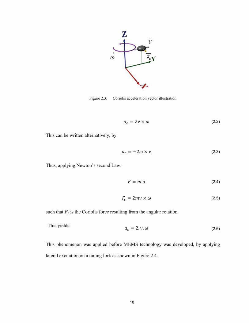
Coriolis Effect occurs for an object moving with linear velocity from a rotating

frame of reference. As an example, assume the rigid body as shown in Figure 2.3 is

moving along the y-axis with linear velocity v along the y-axis. When a rotation exists

around the positive z-axis (considering Faraday’s right hand rule), a resultant Coriolis

acceleration (x-axis direction in this example) will occur perpendicular to both the

rotation axis (z-axis direction) and the linear velocity (y-axis direction). The resultant

Coriolis acceleration is calculated by equation (2.2)

18

2 (2.2)

This can be written alternatively, by

2 (2.3)

Thus, applying Newton’s second Law:

(2.4)

2 (2.5)

such that Fc is the Coriolis force resulting from the angular rotation.

This yields: 2. . (2.6)

This phenomenon was applied before MEMS technology was developed, by applying

lateral excitation on a tuning fork as shown in Figure 2.4.

Figure 2.3: Coriolis acceleration vector illustration

19

If the tuning fork resonates at its first vibration-mode, the fork-tines (i.e. prongs)

move in the same plane but in opposite directions. Coriolis forces will result

perpendicular to the excitation forces because of the rotation around the main axis of the

fork. Thus, by calculating the resultant Coriolis forces or acceleration, the angular

velocity can be calculated.

Scientists and researchers who developed the miniature tuning fork gyroscopes

using the MEMS technology used the same theory of operation as that in the earlier

mechanical one. However, several key parameters had to be taken into consideration due

to the extremely small size and strength of the MEMS structure.

This type of gyroscope uses two vibration mechanisms to measure acceleration.

The first mechanism is excited by the system in order to generate Coriolis forces

accompanying rotation. The second mechanism is a capacitive-based MEMS comb drive

to transform the Coriolis vibrations from the physical mechanical quantity into its

electrical form as a voltage or duty cycle sensor signal. After that, the sensor readings

Figure 2.4: Tuning fork analogy to measure angular rate using Coriolis force

20

are filtered and amplified according to the sensor specifications, using traditional

electronic circuits that are also embedded on the same semiconductor die. Geen and

Krakauer from Analog Devices showed that their iMEMS™ gyroscopes are built upon

the concept of measuring the Coriolis acceleration, as shown in Figure 2.5 [22].

The Analog Device’s inertial measurement sensor ADIS 16355 was chosen for use in

this research because of its relatively low cost and medium accuracy. This MEMS

sensor includes tri-axial gyroscopes, accelerometers and temperature sensors. Moreover,

it is factory-calibrated over its operating temperature range, making the calibration

process more facile [23].

In the instrumentation industry, the specifications of transducers and sensors have

to be strictly adhered to in order to minimize measurement errors. The most significant

specifications for MEMS angular rate gyroscopes were studied, with emphasis on the

Analog Devices ADIS16355 (See Appendix A):

The time domain signals for the three axial gyroscope angular rates and their

discrete trapezoidal integration (i.e. angles) are shown in Figure 2.6 through Figure 2.8.

Figure 2.5: iMEMS gyroscope from Analog Devices™

T

u

The sensors

using the exp

were held a

perimental s

Figure 2.7:

Figure 2.6:

at stationary

set-up discus

Raw angula

Raw angula

21

y position (i.

ssed in Chap

ar rate vs. angu

ar rate vs. angu

.e. zero angu

pter 5.

ular orientation

ular orientation

ular rates) th

n data about y-a

data about x-a

hat was acq

axis

axis

quired

TThe statistics

Angular r

Gx

Gy

Gz

s for the prev

Ta

rate Axis

x

y

z

Figure 2.8:

vious plots a

able 2.1: A

Mean

/

-0.822

0.7879

0.5597

Raw angular r

22

are shown in

Angular rate dat

n

St

9

9

7

rate vs. angula

n Table 2.1

ta-statistics sum

tandard Dev

0.4960

0.6001

0.5181

ar orientation d

mmary

viation

data about z-axi

Varian

0.2460

0.360

0.2684

is

nce

0

1

4

23

The discrete integration process results in Euler’s orientations angles by the

following equations:

(2.7)

(2.8)

(2.9)

Such that is the sampling time, sec for this research. Although the sensor is at

equilibrium, the angle measurements’ histograms show a Gaussian distribution around a

non-zero mean, Table 2.1, showing the static bias (offset) of the gyroscope in the x, y,

and z directions. Thus, the static bias must be calculated before we begin any data

acquisition process.

The gyro static bias calibration was also taken into consideration during the

practical implementation. In order to cancel out these biases, the embedded software

averages the first few samples (100 to 150) at equilibrium, and the output average is

considered the static bias. Next, theses calculated static biases are subtracted from the

forthcoming sensor values. Furthermore, the dynamic biases of the gyroscopes are

estimated using an Extended Kalman Filter to overcome the sudden unnecessary

oscillations [24]. The output of the unbiased angular rates as well as the resulting angles

showed relatively better results than raw data calculations, Figure 2.9.

m

f

m

Howe

misalignmen

fusion betw

magnetomet

Figure

ever, since d

nt, and senso

ween multipl

ters – had to

2.9: Angula

dynamic drif

or-temperatu

le inertial s

be consider

24

ar rate data afte

ft, noise du

ure response

sensors – th

ed.

er static bias co

e to linear a

inject rando

hat is, Gyro

ompensation

acceleration

omness in th

oscopes, acc

s, manufact

he system, se

celerometers

turing

ensor

s and

25

2.1.2 MEMS Capacitive Accelerometers

Mechanical accelerometers are used in many applications. Their mechanical structure has

a proof mass with an attached needle and a spring, analogous to weighing instruments of

the past. The mechanical model of an accelerometer, with its approximate mass spring

and damper equivalent, is shown in Figure 2.10. The differences between forces acting on

the mass are proportional to the linear acceleration.

The spring exerts a force of

(2.10)

Where K is the spring constant, x is the travelled distance, and F is the spring reaction

force. The damping force is

(2.11)

This equation obeys Newton’s second Law :

Figure 2.10: Accelerometer approximated mass-spring model

26

(2.12)

The above equations are combined to form the second-order differential equation for

displacement x as:

0 (2.13)

This yields: 2 0 (2.14)

Where the undammed natural frequency is

/ (2.15)

and the damping ratio is: 2√ (2.16)

MEMS accelerometer designs more or less follow this same design concept. A

proof mass is suspended over a small gap on the end a cantilever or hanging from a

membrane flexible structure. Figure 2.11 shows the difference in the MEMS structure

between a Piezo-resistive accelerometer and a capacitive accelerometer.

27

In the Piezo-based system, the deflection is less than the capacitive, which provides more

sensitivity – up to 1 , where g is the gravitational acceleration. However, this reduces

the overall measurement dynamic range of the sensor and obliges the designer to consider

a relatively large proof mass. Furthermore, capacitive accelerometers are less vulnerable

to temperature changes than the Piezo-resistive systems.

In addition, the electronic circuitry needed to convert mechanical acceleration to

an electrical signal is simple in Piezo-resistive accelerometers, because Piezo electric

materials generate voltages proportional to the applied stress. On the other hand,

capacitive MEMS accelerometers need a more complex circuitry involving alternating

voltages and modulation/demodulation electronics, as shown in Figure 2.12 [25].

Figure 2.11: Piezo-resistive vs. capacitive accelerometers structure

28

Tilt angle measurement using accelerometer values depends entirely on the gravitational

acceleration. However, this is not the case for dynamic bodies or systems, where linear

accelerations are added to the measured data.

The inertial frame for the body segment or the sensor is given with respect to

Earth’s-Centered-Earth-Fixed (ECEF) frame, as shown in Figure 2.13. The frame

assignment used in this research follows the conventional one used in aviation [26].

Assuming that the arm is held horzointal to earth, the positive x-axis points towards the

elbow of the human arm from the shoulder’s joint prespective, the positive z-axis points

downwards towards earth, and the positive y-axis is to the right of the right arm, also

known as Local Tangent Plane (LTP).

Figure 2.12: MEMS accelerometer internal circuit (Analog Devices™)

29

The time domain three-axes accelerations and their corresponding static biases

acquired by the analog devices ADIS16355 [23] are shown in Figure 2.14 through Figure

2.16. These experimental results were also taken at the equilbirum state of the sensor held

horizontally, measuring normalized accelerations due to gravity; that is, ax=ay=0, and

az=1 using the developed sensor module discussed in Chapter 5.

Figure 2.13: ECEF Vs sensor coordinate frame

30

0 5 10 15 20 25-0.1

-0.08

-0.06

-0.04

-0.02

0

0.02

0.04

0.06

0.08

Time (seconds)

Am

plitu

de

(Norm

aliz

ed

over g

ravi

ty)

X-Axis Acceleration (Time Domain)

X-Axis Acceleration

-0.2 -0.15 -0.1 -0.05 0 0.05 0.1 0.15

500

1000

1500

2000

2500

Amplitude (Normalized over gravity)

Num

ber o

f Hits

X-Axis Acceleration (Histogram)

X-Axis AccelerationGaussian Fit

Bias

0 5 10 15 20-0.1

-0.08

-0.06

-0.04

-0.02

0

0.02

0.04

0.06

0.08

0.1

Time (seconds)

Am

plit

ud

e (N

orm

aliz

ed

ove

r g

ravi

ty)

Y-Axis Acceleration (Time Domain)

Y-Axis Acceleration

-0.1 -0.05 0 0.05 0.1

500

1000

1500

2000

2500

3000

3500

Amplitude (Normalized over gravity)

Nu

mb

er

of H

its

Y-Axis Acceleration (Histogram)

Y-Axis Acceleration

Gaussian Fit

Bias

Figure 2.15: Raw linear acceleration along y-axis with sensor module fixed

Figure 2.14: Raw linear acceleration along x-axis with sensor module fixed

31

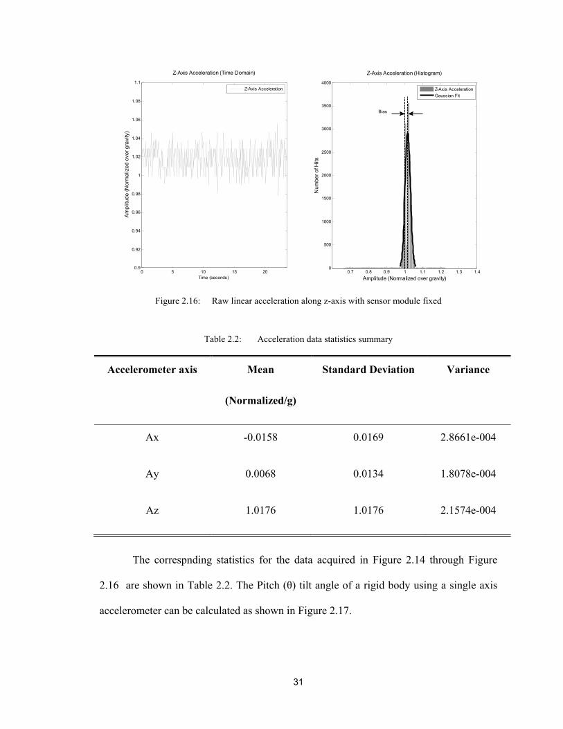
Figure 2.16: Raw linear acceleration along z-axis with sensor module fixed

Table 2.2: Acceleration data statistics summary

Accelerometer axis Mean

(Normalized/g)

Standard Deviation Variance

Ax -0.0158 0.0169 2.8661e-004

Ay 0.0068 0.0134 1.8078e-004

Az 1.0176 1.0176 2.1574e-004

The correspnding statistics for the data acquired in Figure 2.14 through Figure

2.16 are shown in Table 2.2. The Pitch (θ) tilt angle of a rigid body using a single axis

accelerometer can be calculated as shown in Figure 2.17.

0 5 10 15 200.9

0.92

0.94

0.96

0.98

1

1.02

1.04

1.06

1.08

1.1

Time (seconds)

Am

plit

ud

e (

No

rma

lize

d o

ver

gra

vity

)

Z-Axis Acceleration (Time Domain)

Z-Axis Acceleration

0.7 0.8 0.9 1 1.1 1.2 1.3 1.40

500

1000

1500

2000

2500

3000

3500

4000

Amplitude (Normalized over gravity)

Nu

mb

er

of H

its

Z-Axis Acceleration (Histogram)

Z-Axis Acceleration

Gaussian Fit

Bias

32

The following simple vector relation can be used to obtain the the pitch angle as:

The same method can be used to calculate Roll angle (φ) by using a second

orhtognally mounted accelerometer. However, a combination of all three accelerometers

can be used to pinoint accurately the three Euler angles of the sensor’s coordinate frame.

These required angles are obtained by applying the following relations [27]:

For the Roll angle:

(2.18)

such that the normalized vector

is the normalized y-axis accelerometer data

over earth’s gravity (i.e. 9.8 m/sec2).

Also

(2.17)

Figure 2.17: Pitch angle measurement theory using single axis accelerometer

33

Dividing both equations in the L.H.S. vector in equation (2.18) yields

(2.19)

and therefore (2.20)

Nevertheless, a problem is introduced by using the atan function: The quadrant

determination of the angle cannot be determined accurately unless the corresponding

two-argument arc tan one (i.e. atan2 ) is used. This method limits the angle range

between +180 and -180 degrees. Knowing that the two-argument arc tan function can be

defined using:

For y≠0 2 ,

· ; 0

2· ; 0

· ; 0

And For y=0 2 ,0 ; 0

; 0 ; 0

Such that is the angle and tan . Also sgn is the mathematical sign function.

Also the atan2 function can be expressed interms of arc tan half angle function as:

2 , 2

2 (2.21)

Similarily The pitch angle can be obtained using the two equations:

34

(2.22)

Following the same methodology to obtain equation (2.21), the pitch angle is obtained

by:

2 , (2.23)

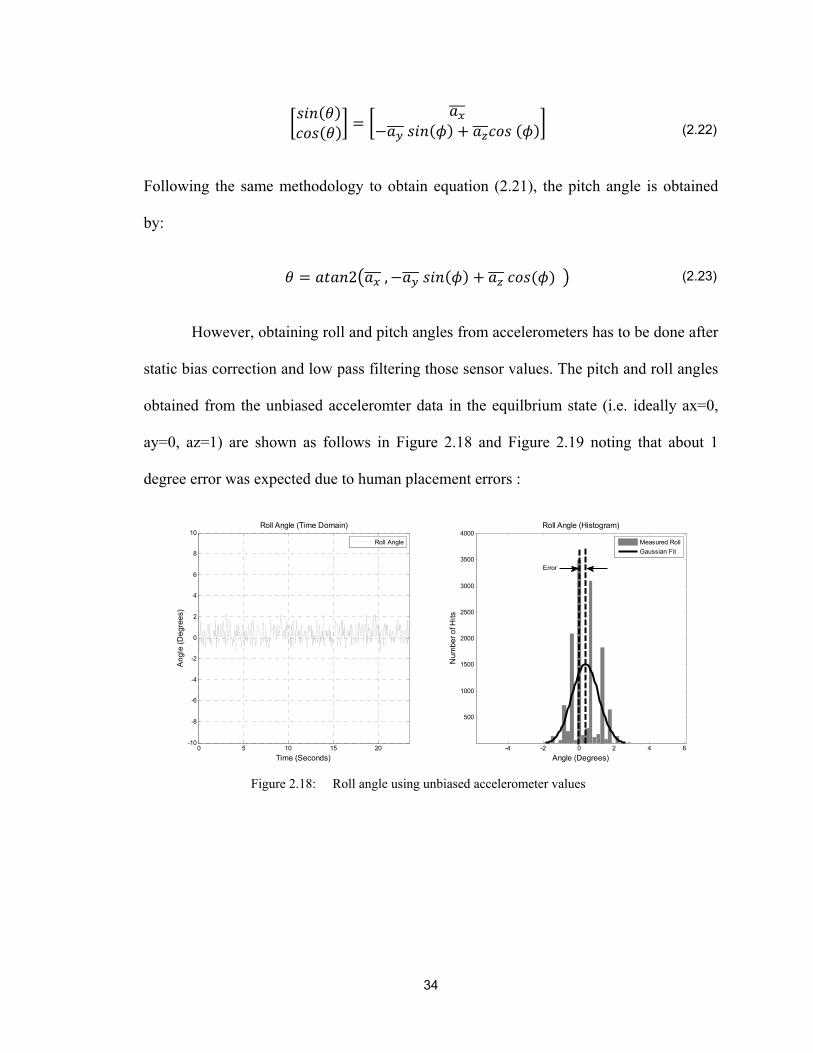
However, obtaining roll and pitch angles from accelerometers has to be done after

static bias correction and low pass filtering those sensor values. The pitch and roll angles

obtained from the unbiased acceleromter data in the equilbrium state (i.e. ideally ax=0,

ay=0, az=1) are shown as follows in Figure 2.18 and Figure 2.19 noting that about 1

degree error was expected due to human placement errors :

0 5 10 15 20-10

-8

-6

-4

-2

0

2

4

6

8

10

Time (Seconds)

Ang

le (

Deg

ree

s)

Roll Angle (Time Domain)

Roll Angle

-4 -2 0 2 4 6

500

1000

1500

2000

2500

3000

3500

4000

Angle (Degrees)

Num

ber o

f Hits

Roll Angle (Histogram)

Measured Roll

Gaussian Fit

Error

Figure 2.18: Roll angle using unbiased accelerometer values

35

The statistical analysis summary for Figure 2.18 and Figure 2.19 is shown in Table 2.3.

Table 2.3: Roll and pitch angles' statistics calculated using accelerometers

Angle Mean

Standard Deviation Variance

Roll (Φ) 0.3814 0.7575 0.5737

Pitch (θ) 0.8923 0.9537 0.9096

The large variance value for the pitch angle is due to the external vibrational

noises in the laboratory during the experiment.

Nevertheless, the Yaw angle – heading angle around the z-axis – cannot be

calculated using accelerometers, because of the semmetry of eath’s magnetic field while

0 5 10 15 20-10

-8

-6

-4

-2

0

2

4

6

8

10

Time (Seconds)

An

gle

(Deg

rees

)

Pitch Angle (Time Domain)

-12 -10 -8 -6 -4 -2 0 2 4 6 80

500

1000

1500

2000

2500

Angle (Degrees)

Nu

mbe

r o

f Hits

Pitch Angle (Histogram)

Measured Pitch

Gaussian Fit

Pitch Angle

Error

Figure 2.19: Pitch angle using unbiased accelerometer values

36

rotating around that axis. This fact introduces the use of magnetometers as a heading

measuring sensors to calculate the yaw angle with respect to earth’s magnetic north.

2.1.3 MEMS Magnetometers

Earth’s magnetic field is considered relatively small, ~0.5 to 0.6 Gauss. Chinese

historical literature shows that the magnetic compass was used for navigation as early as

the fourth century BC. Later, the principles upon which a magnetometer depends were

classified into either mechanical, magneto-resistive, Hall Effect, and magneto-inductive.

The magneto-inductive magnetometer type was chosen for use in this project because of

its low cost and small size. The general theory of operation to measure magnetic field

using inductance dates to 1831, when British scientist Michael Faraday discovered

electromagnetic induction.

Faraday developed his law through observing a voltage change in a coil wrapped

around a soft-iron core loop when voltage was applied to another nearby coil. Later, these

proofs of concept led to the invention of the transformer. Magneto-inductive sensors can

be simplified based on Faraday’s experiment. However, several noise sources can

dramatically affect a magnetometer reading; these include temperature change, and

surrounding electromagnetic interference due to sources or iron cores. The PNI-11096

(Appendix B) magneto-inductive sensor driver ASIC chip applies an oscillator o/p into an

end of a coil parallel to the magnetic sensitive axis while grounding the other end of the

coil. Furthermore, a counter counts the time taken for a predetermined oscillations

number. Next, the same measurement is done after switching the coil terminals, as shown

in Figure 2.20 [28].

37

This differential method of calculation reduces vulnerability to temperature change.

The following trigonometric relation can be used to calculate yaw angle ψ (Heading)

using a minimum dual-axis magnetometer held parallel to earth’s horizon:

(2.24)

(2.25)

One way for the processor to keep track of the angle is to apply the following constraints:

Heading angle ψ= 90-[arc tan(x/y)*180/π] By>0

Heading angle ψ= 270-[arc tan(x/y)*180/π] By<0

Heading angle ψ= 180 By=0 & Bx<0

Heading angle ψ= 0 By=0 & Bx>0

These relationships are applied due to the fact the vector field strengths

surrounding earth are almost planar near the equator, but as they approach the poles the z-

component appears. It should be known that earth’s geographic north is not the same as

Figure 2.20: Forward /Reverse bias (courtesy of PNI™ Corp.)

38

its magnetic north. Furthermore, compass readings point towards the magnetic north. The

angular offsets between compass north, magnetic north and geographic north are shown

in Figure 2.21 [27].

Where declination angle is denoted by δ and the heading angle by ψ.

It is also worth noting that the magnetic declination angle δ changes with both the

position on earth’s surface (longitude and latitude) and time. For simplicity in this

research, magnetic north is considered the reference to the yaw angle. To refer to true

north, one can use the World Magnetic Model (WMM) whenever the sensory system is

moved to a new location to find the declination angle.

Figure 2.22 through Figure 2.24 show the normalized magnetic field flux density

readings for the x-, y- and z-axis, and their histograms sampled using the PNI-

MicroMag3 tri-axes magnetometer at stationary position pointing towards about 95

degrees from Magnetic North (± 1-degree error due to human placement and axes

misalignments).

Figure 2.21: Geographic, Magnetic north versus sensor heading angle

39

0 5 10 15 20-0.06

-0.055

-0.05

-0.045

-0.04

-0.035

-0.03

Time (seconds)

No

rmal

ize

d M

ag

ne

tic F

lux

Den

sity

X-Axis Magnetic Field Flux Density (Time Domain)

-0.1 -0.08 -0.06 -0.04 -0.02 0 0.02

2000

4000

6000

8000

10000

12000

Normalized Magnetic Flux Density

Nu

mb

er o

f Hits

X-Axis Magnetic Field Flux Density (Histogram)

X-Axis Magnetic Flux Density

Gaussian FitX-Axis Magnetic Flux Density

0 5 10 15 20-0.4

-0.39

-0.38

-0.37

-0.36

-0.35

-0.34

-0.33

-0.32

-0.31

-0.3

Time (seconds)

No

rma

lize

d M

ag

ne

tic F

ield

Flu

x D

en

sity

Y-axis Magnetic Field Flux Density (Time Domain)

-1 -0.8 -0.6 -0.4 -0.2 0 0.2

2000

4000

6000

8000

10000

12000

Normalized Magnetic Field Flux Density

Nu

mb

er

of H

its

Y-axis Magnetic Field Flux Density (Histogram)

Y-Axis Magnetic Flux Density Y-Axis Magnetic Flux Density

Gasussian Fit

Figure 2.23: Normalized magnetic flux density in the y-axis

Figure 2.22: Normalized magnetic flux density in the x-axis

40

The corresponding statistical parameters are stated in Table 2.4.

Table 2.4: Magnetometer data statistics summary

Magnetometer

axis

Mean

(Normalized/Magnitude)

Standard

Deviation

Variance

Mx -0.0454 0.0031 9.3357e-006

My -0.3485 0.0212 1.7240e-004

Mz 0.9355 0.0302 9.1179e-004

0 5 10 15 20 25

0.932

0.934

0.936

0.938

0.94

0.942

Time (seconds)

No

rma

lize

d M

ag

ne

tic F

ield

Flu

x D

en

sity

Z-Axis Magnetic Field Flux Density (Time Domain)

Z-Axis Magnetic Field Flux Density

0.2 0.4 0.6 0.8 1 1.2 1.4

2000

4000

6000

8000

10000

12000

14000

Normalized Magnetic Field Flux Density

Nu

mb

er

of H

its

Z-axis Magnetic Field Flux Density (Histogram)

Z-Axis Magnetic Field Flux Density

Gaussian Fit

Figure 2.24: Normalized magnetic flux density in the z-axis

41

In order to perform a magnetometer calibration against surrounding magnetic

disturbances, usually the sensor is rotated two complete turns around its vertical axis.

Figure 2.25 shows the corresponding oscillation counts resembling the magnetic field

flux density given by the magnetometers by performing multiple 360-degree turns. It

shows the effect of soft iron and hard iron magnetic disturbances surrounding the sensor,

generating inconsistencies.

Since the previous results assume a perfect horizontal orientation of the

magnetometer, heading errors are induced. Gebre Eghziabher [29] showed a method to

combine accelerometers and magnetometers integrated with baseline attitude and GPS to

calculate orientation parameters without the use of gyroscopes. Furthermore, the method

introduced by Bekir [27] was used to obtain the magnetic heading angle (yaw) by

combining magnetometers and accelerometer sensors. The algorithm to obtain the yaw

angle depends on obtaining the angle towards magnetic north after compensating the tilt

Figure 2.25: Magnetic flux density frequency counts performing 360 loops

42

effects on the magnetometers. The following equations can solve the tilt compensation

problem of the magnetometer readings using the accompanying accelerometers:

Assuming the vector P is the output vector from the cross product between the

acceleration vector and the magnetic field vector,

(2.26)

and yields (2.27)

Following the same concept as the Pitch and Roll angles to convert the tan

function to specify quadrants, the Yaw and angle are given by:

2 , (2.28)

The output of equation (2.28) using the sampled data with the sensor almost

pointing towards 95 degrees from magnetic north is shown in Figure 2.26 (the design of

the sensor can be seen in Chapter 5).

43

The statistics for Figure 2.26 are stated in Table 2.5:

Table 2.5: Yaw angle statistics summary

Orientation angle Mean Standard deviation Variance

Ψ 95.0572 2.5607 6.5572

0 5 10 15 20 2585

90

95

100

105

110

115

Time (Seconds)

An

gle

(D

eg

ree

s)

Yaw Angle (Time Domain)

Yaw Angle

75 80 85 90 95 100 105 110 115 120

200

400

600

800

1000

1200

1400

1600

1800

Amplitude (Degrees)

Nu

mb

er

of H

its

Yaw Angle (Histogram)

Measured Yaw

Gaussian Fit

Figure 2.26: Heading angle output using tilt compensated magnetometers

44

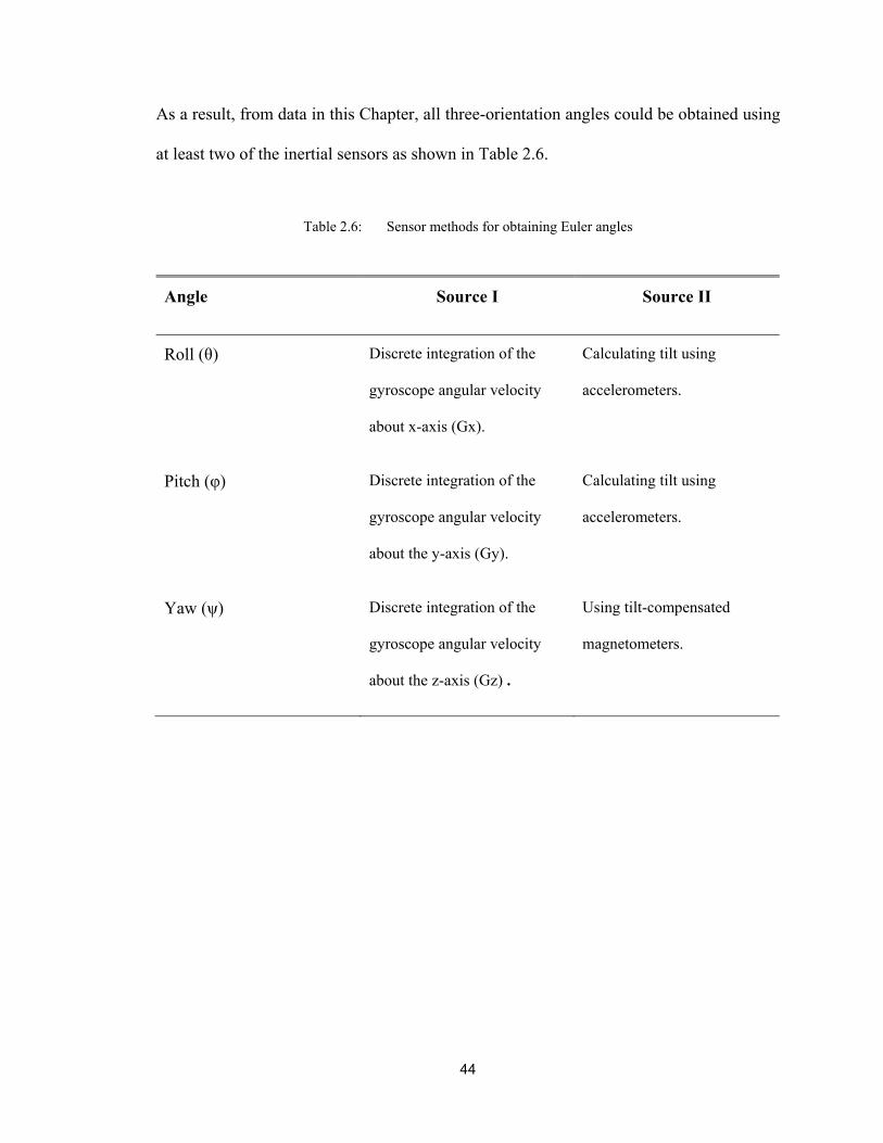
As a result, from data in this Chapter, all three-orientation angles could be obtained using

at least two of the inertial sensors as shown in Table 2.6.

Table 2.6: Sensor methods for obtaining Euler angles

Angle Source I Source II

Roll (θ) Discrete integration of the

gyroscope angular velocity

about x-axis (Gx).

Calculating tilt using

accelerometers.

Pitch (φ) Discrete integration of the

gyroscope angular velocity

about the y-axis (Gy).

Calculating tilt using

accelerometers.

Yaw (ψ) Discrete integration of the

gyroscope angular velocity

about the z-axis (Gz) .

Using tilt-compensated

magnetometers.

45

2.2 Orientation Determination

The Euler angles (θ, φ and ψ) are sufficient to express orientation and rotation in three-

dimensional space using several representation methods – Directional Cosine Matrix,

Euler’s axis-angle, Euler rotations and Quaternions.

The most common methods, directional cosine matrix and quaternion, were

studied as follows.

2.2.1 Orientation Determination using Directional Cosine Matrix

As the name implies, each element of the directional cosine matrix is the cosine of the

angle between an axis of the three axes of the body’s frame at a given point in time and

the reference unit axis. The coordinate frame used here is a local frame with respect to

the sensor body. The x, y and z unit vectors point towards front, right and down of each

sensor (Local NED frame).

The two-dimensional clockwise rotation of the sensor in space around its z-axis

with an angle ψ (heading angle) the rotation matrix is given by:

(2.29)

Matrix R has the properties: . 1

Extending the rotation to a three-dimensional spatial one, the rotation matrices about each

of the three basis axes are shown next.

The pure rotation around x-axis (Roll) is given by:

46

1 0 000

(2.30)

and the rotation around the y-axis (Pitch) is given by:

00 1 0

0 (2.31)

Finally, the rotation around the z-axis (Yaw or change in heading angle) is given by:

00

0 0 1 (2.32)

Representation of rotation in three-dimensional Euclidean space can be obtained

using multiplication of the matrices shown in equations (2.30) thorough (2.32). For

instance, the rotation of the inertial sensor around the z-, y- and x-axis can be calculated

as:

, , . .

(2.33)

such that the abbreviations , , and so on for the remaining

angles.

47

But to obtain Euler angles from the Directional Cosine Matrix (DCM), we have:

2 ,

2 ,

(2.34)

This means that by using the three Euler angles φ, θ and ψ, different combinations

of matrix multiplications other than the previous equation can be used to express rotation.

Different rotation sequences can be (x, y, z), (x, z, y), (y, x, z), (y, z, x), (z, x, y) and (z, y,

x), which make about six combinations; the angles are dependent, which means that any

two 90-degrees rotation about two axes can be expressed as one 90-degree rotation

around the third axis. Furthermore, one can express three-dimensional rotations by using

only two of three rotation matrices by rotating the body about the first axis, then the

second, then the first again, as in (z, x, z), (z, y, z), (y, x, y), (y, z, y), (x, y, x) and (x, z,

x).

This exercise raises the number of combinations to 12. Moreover, one can choose

between the reference frame to be either the previous local coordinate frame (relative

coordinates) or earth’s fixed frame (absolute coordinates), increasing the possible

combinations to 24.

Several drawbacks appear when representing orientation using directional cosine

matrices (Rotation Matrix), such as computation complexity and Gimbal-lock [30]. A

well-known solution to these problems is to use quaternions.

48

2.2.2 Orientation Determination using Quaternions

Quaternions were invented by Sir. William Rowan Hamilton in 1843 as an attempt to

generalize complex numbers to include three-dimensional space. A quaternion is

represented as one scalar and three vector parts [30]:

(2.35)

where q0 is the scalar part and q1, q2 and q3 are the three elements of the vector part. The

vector part of the quaternion obeys the rule:

1 (2.36)

The same quaternion can also be presented as:

, or ,

such that is the scalar component, and is the three-dimensional vector component.

Also, θ is the angle and n is the unit vector pointing along the direction of the

rotation axis following the angle-axis Euler convention.

Quaternions can be represented in their matrix form [30] as:

(2.37)

To express a pure rotational transformation between two coordinate frames using

quaternions, a quaternion multiplication takes place as:

49

, , , , , ,

(2.38)

Quaternion algebra is similar to vector algebra except for multiplication. The

transformation between the Directional Cosines Matrix, Euler’s axis-angle and

quaternion form can be done quite easily. In order to calculate quaternion orientation

using Euler angles, the following equation is used:

2 2 2 2 2 2

2 2 2 2 2 2

2 2 2 2 2 2

2 2 2 2 2 2

(2.39)

Given that q1, q2, and q3 are the vector components that the coordinate frame rotated

about. Also, q0 is the scalar part of the quaternion expressing the angle that body rotated

about. The quaternion to DCM rotation matrix is transformed using:

2 22 22 2

(2.40)

50

knowing that the quaternion used in the transformation is a normalized quaternion by:

(2.41)

such that:

By analogy to equation (2.34), the transformation of quaternion notation back to Euler

angles, the equation used is:

2 2 ,2

2 2 ,

(2.42)

These relations result in angle values in units of radians.

An estimation algorithm was considered in the research because of the bias, drift

errors, and random noise effects noticed on the orientation angles acquired earlier in this

chapter. A literature review showed that the conventional estimator used in aerospace and

computer graphics to estimate the quaternion (Orientation) state of a coordinate frame is

the Extended Kalman Filter.

51

Chapter 3: ATTITUDE ESTIMATION USING EXTENDED KALMAN FILTER

In this research, attitude estimation using the extended Kalman Filter (EKF) is used for

sensor fusion between the inertial sensors because the previous results from the

equilibrium state experiment shown in Chapter 2 clarify the effect of gyroscope drift

problems due to integration of noise. Other systems’ noise-related factors are temperature

variation, misalignment errors, and miscalculated biases. Furthermore, since angular

velocities obtained from gyroscopes are integrated to produce angles to express

orientation, the initial conditions have to be known. A solution to that problem is to use

the angles obtained from accelerometers and magnetometers as the initial conditions.

Based on optimal estimation theory, the Extended Kalman Filter is a recursive

optimal estimator that can be used for non-linear system state estimation [26]. Two

Extended Kalman Filter designs were studied and implemented to estimate the

orientation of each sensor module.

52

3.1 Sensor Measurement Models

The measurement modeling phase is a critical step in order for the Kalman

Filter/estimator to operate accurately. The sensors’ measurement models are discussed

for each sensor as follows:

3.1.1.1 Gyroscope Measurement Model

The angular velocity model of the gyroscope can be expressed by equation (3.1),

(3.1)

such that:

is static gyroscope biases (offset)

(3.2)

which expresses the measured angular velocities vector using the gyroscope triplet group.

Also (3.3)

Vector is the dynamic bias vector for each of the three axes’ measured angular rates.

In addition, is the noise vector.

53

On the other hand, a set of sensor data is averaged by the software algorithm at

the beginning of each data acquisition session to compute static biases, as stated in

Chapter 2. Then, each sensor measurement is subtracted from the calculated static bias

(offset) using:

(3.4)

The noise statistical parameters for the gyroscope measurements were calculated

experimentally using reference data due to equilibrium. Noise is modeled as the zero-

mean uncorrelated white Gaussian noise , and variances are used for initializing the

covariance matrices in the EKF algorithm.

The measurement model expressed by equation (3.1) does not take sensor

misalignments, temperature compensation and cross-axis dependencies into

consideration. This assumption was used because of the nature of the MEMS gyroscopes

embedded in the analog device’s inertial measurement unit (ADIS16355) being used,

which has minimal misalignment errors as well as temperature compensation throughout

its temperature range (Appendix A).

54

3.1.1.2 Accelerometer Measurement Model

The measurement modeling equation for the accelerometer reading is:

(3.5)

(3.6)

The vector is the accelerometer’s measured values vector. Also the

vector is the bias vector, and is the noise vector by analogy to the gyroscope’s

measurement model.

The static bias vector affects tilt measurement for the magnetometer

compensation as well as measures both the Roll angle and the Pitch angle in the EKF.

This static bias is also computed by averaging the first set of data measurements before

any acquisition session, by analogy to the gyroscope static biases.

Furthermore, other models include the compensation due to earth’s centripetal

acceleration with the accelerometer and gyroscope models. However, since this

acceleration is so small that low-cost sensors cannot sense it, it was not considered during

the modeling.

Accelerometer measurement noise was analyzed in order to use the variance in

the EKF measurement covariance matrices initialization.

55

3.1.1.3 Magnetometer Measurement Model

The equation governing each of the three magnetometers can be expressed by:

(3.7)

such that: (3.8)

The vector is the actual sensor values streaming from the magnetometer

triad. Furthermore, vector includes the magnetic disturbances that affect measuring

true magnetic field of earth. Magnetic noise can be classified into the so-called soft iron

and hard iron interferences [31]. The soft iron disturbances are induced through the

reflection of magnetic and electromagnetic field applications. The hard iron disturbances

are external magnetic fields generated by the surrounding sources such as transformers,

lighting systems, cellular phones and iron core materials. Accelerometer tilt

measurements are used to compensate for the magnetic dip-angle effect on the

magnetometers, as described in previous chapters. In addition, other noise sources are

modeled as , zero-mean uncorrelated white Gaussian noise.

56

3.2 Euler-based Orientation Estimation Algorithm

This algorithm uses the measured Euler angles given by accelerometers and

magnetometers to compensate for the gyroscope’s dynamic drift. Experiments also

showed that it is advantageous to add more dependency on the gyro-based orientation

angles in dynamic states. On the other hand, Euler angles should be calculated using

accelerometers and magnetometers in static and slowly moving states.

3.2.1 Euler Angles Estimator Design

A rotational transformation between two successive frames in time can be expressed by

the differential equation. The measured angular velocities p, q and r relate to the angular

velocities in terms of Euler angles [26] by:

10

0

(3.9)

such that s, c, and t are abbreviations for the sine, cosine, and tan functions respectively.

57

3.2.1.1 System State Model

The system state vector to be estimated is composed of the six elements: the three Euler

angles and three dynamic biases of the gyroscope, as shown in:

.

(3.10)

To determine the state transition matrix F, the Jacobian of equation (3.9) is derived as:

, , , , ,

(3.11)

The system state noise is modelled as the Gaussian noise with zero mean and variance

Q ( 0, ). The covariance matrix Q holds the variances of the state vector

elements in the three frame axes, assuming decoupled effects as follows:

58

00 (3.12)

such that :

0 0

0 00 0

and

0 0

0 0

0 0

The values of these variances were calculated experimentally by keeping the sensor in

equilibrium for a sufficient time and studying its statistical characteristics.

3.2.1.2 System Measurement Model

The measurement model is composed of the Euler angle measurements corrupted with

the noise vector shown as:

000

(3.13)

The Euler angles acquired here are roll (φ) and pitch (θ) from accelerometers, and

Yaw (ψ) from the tilt compensated magnetometers. Also, vk is the measurement noise

modeled as Gaussian noise with zero mean and variance R (i.e. 0, ). The

measurement covariance matrix R is given in (3.13):

59

00 0 (3.14)

3.2.1.3 Prediction and Update

Prediction starts by estimating the system state using:

· (3.15)

The system state error covariance estimate (Continuous time update) is:

· · (3.16)

The error covariance is then updated by:

· (3.17)

such that Ts is the sampling time.

Furthermore, the Kalman Gain is determined through the following relation:

· · · (3.18)

The update phase of the Kalman Filter algorithm is made by using the following

two equations:

· (3.19)

60

such that the “ ” term is calculated as the difference between the measured Euler

angle and its estimated value given from the previous state.

· · (3.20)

3.2.2 Estimator Experimental Results

Practical results showed that the estimated roll and pitch angles converge efficiently to

the reference ones. However, the yaw angle showed instabilities because the lab

environment has affected the modeling statistics of the magnetometers by hard and soft

iron disturbances. The experimental results are shown in Figure 3.1 through Figure 3.6,

comparing the performance of the developed sensor with the performance of an

industrial-grade AHRS (Microstrain GX2). The developed inertial sensor module was

fixed onto the reference AHRS as shown in Chapter 5 section 3.

Figure 3.1: Estimated-roll using Euler-based EKF

0 10 20 30 40 50 60 70 80 90 100-200

-150

-100

-50

0

50

100

150Performance of Euler-Based EKF for Roll Angle Estimation

Time (Seconds)

An

gle

(D

eg

ree

s)

MeasuredRef. (GX2)EKF Output

61

In order to show the Euler-based EKF performance more efficiently, a zoomed-in

version on the time interval between the 50th and the 60th seconds is shown in Figure

3.2.

Figure 3.2: Zoomed estimated-roll angle using Euler-based EKF

Continuing using the same scheme of figures, the Pitch angle EKF performance is

shown in Figure 3.3 and the selected time-interval zoom-in is shown in Figure 3.4.

Figure 3.3: Estimated-pitch using Euler-based EKF

51 52 53 54 55 56 57 58 59 60

-40

-30

-20

-10

0

10

20

30

40

50Performance of Euler-Based EKF for Roll Angle Estimation

Time (Seconds)

An

gle

(Deg

ree

s)

MeasuredRef. (GX2)EKF Output

0 10 20 30 40 50 60 70 80 90 100-80

-60

-40

-20

0

20

40

60

80Performance of Euler-Based EKF for Pitch Angle Estimation

Time (Seconds)

Ang

le (

Deg

rees

)

Measured

Ref. (GX2)EKF Output

62

Figure 3.4: Zoomed estimated-pitch angle using Euler-based EKF

Figure 3.5: Estimated-yaw angle using Euler-based EKF

50 51 52 53 54 55 56 57 58 59-20

-10

0

10

20

30

Performance of Euler-Based EKF for Pitch Angle Estimation

Time (Seconds)

Ang

le (

Deg

rees

)

Measured

Ref. (GX2)EKF Output

0 10 20 30 40 50 60 70 80 90 100-150

-100

-50

0

50

100

150Performance of Euler-Based EKF for Yaw Angle Estimation

Time (Seconds)

Ang

le (

De

gre

es)

Measured YawReference (GX2)EKF-Yaw Output

63

Lastly, the zoomed time-interval-section from Figure 3.5 is shown in Figure 3.6.

Figure 3.6: Zoomed estimated-yaw angle using Euler-based EKF

The error analysis studies for the previous results are summarized in Table 3.1:

Table 3.1: Error analysis for the Euler-based EKF estimator results

Orientation Angle Error Mean Error (deg)

φ 3.2287

θ 2.9146

Ψ 10.8224

Singularities form a major problem that appears when using Euler angles. The

system singularities are at a pitch angle of ±90 degrees because the roll angle will be in

phase with the yaw axis. Another reason is that at these pitch angles, accelerometer axes

z and y will be perpendicular to earth’s gravity vector, causing the trigonometric

51 52 53 54 55 56 57 58 59 60

-120

-100

-80

-60

-40

-20

0Performance of Euler-Based EKF for Yaw Angle Estimation

Angle

(D

egre

es)

Measured YawReference (GX2)EKF-Yaw Output

64

functions to divide by zero, resulting in singularities. A common solution for this

problem is to use quaternions.

3.3 Quaternion-based Orientation Estimation Algorithm

The EKF used here acts as a complementary/indirect filter to the general kinematics

calculation algorithm because it focuses on error analysis as well as the state estimation.

The estimator structure, system state space model and results are shown in the sequence

presented throughout this chapter.

The extended EKF was applied to combine the three-dimensional accelerometers,

magnetometer and gyroscopes sensor data.

The accelerometer measurements and magnetometer measurements are combined

to cancel out the tilt affecting magnetometer readings using the acceleration due to

earth’s gravity. Furthermore, data of all the nine sensors are sent simultaneously to the

extended Kalman Filter estimator. Then the estimator relies on the statistics calculated

prior to the experiment during the calibration phase to adjust the gains weighing the

system dependence on sensor values for each orientation angle based on the nature of the

motion with respect to the error analysis.

65

3.3.1 Quaternion Estimator Design

The equation relating the derivatives of the quaternion to the angular velocities [26] is

given by:

00

00

(3.21)

This data can also be written

as: 12

· , , · (3.22)

such that the angular velocity matrix , , can be driven in terms of the gyroscopes

measurements as:

, ,

00

00

(3.23)

This relation is used in the software algorithm to update the orientation state vector in the

discrete form using:

(3.24)

Where is the updated quaternion state at time step k+1, and Ts is the sampling time.

66

3.3.1.1 System State Model

The state vector used in this research is composed of a quaternion along with the dynamic

gyroscope biases, as expressed by (3.25) and (3.26).

· (3.25)

such that the state vector is (3.26)

The vector corresponds to the derivative of the state vector, given that the

gyro-dynamic biases , and are constants, leading their derivatives to be zeros as

shown in (3.27).

000

(3.27)

Also, F is the system state transition matrix of the quaternion calculated as:

(3.28)

The function is defined as the Jacobian of the state vector at time step k+1

with respect to the state vector at time step k.

67

This leads the state transition function F to be as shown in (3.29).

12

00

00

0 0 0 0 0 0 00 0 0 0 0 0 00 0 0 0 0 0 0

(3.29)

The vector in the state model resembles the error vector. It is also characterized by the

system states error covariance matrix Q as:

0 00 · (3.30)

The scalar value denotes the variances of the gyroscopes calculated by obtaining the

angular rate data in static conditions. In this case, it is assumed to be the variance of the

dynamic gyro-biases, too.

68

3.3.1.2 System Measurement Model

Following the same procedure taken in designing the system state model, the

measurement model is:

(3.31)

Vector denotes the error measurements, and it is updated with every iteration to

correct the state vector given the measured quaternion and Euler angles. The sequence of

this updating procedure is discussed in the next section.

The noise is modeled as white Gaussian noise with zero mean and variance

R (i.e. 0, ). The measurement covariance matrix R is composed of the

variances of the measurements, that is, variances of the Euler angles. For practical

experiments, these variances are assumed to be 1 because of external magnetic

interferences affecting the calculation of variances, specifically the yaw angle.

These preliminary results show that the orientation angles are better obtained

using magnetometers and accelerometers in steady state. Nevertheless, the gyroscope

results showed more efficiency in the dynamic states because of the addition of linear

acceleration to the accelerometers.

3.3.1.3 Prediction and Update

The prediction and update steps are made using the following set of equations [31]:

Prediction starts by estimating the system state using:

· (3.32)

69

The system state error covariance estimate is:

· ·

(3.33)

The update phase of the estimator uses a sequence of the Euler angles measurements. The

error measurements are updated as:

Roll error update:

2 2

(3.34)

Pitch error update:

(3.35)

Yaw error update:

2

2

(3.36)

The terms , and are calculated from the estimated quaternion

via the directional cosine matrix (DCM). Equations (3.37) through (3.39) show the

procedure of calculating those angle errors.

70

2 (3.37)

2

1 (3.38)

2 (3.39)

Continuing the update phase, the error covariance is then updated by:

·

(3.40)

We see that the Kalman Gain is determined through:

· · · (3.41)

Next, the state vector update is given by:

(3.42)

It is worth noting that the quaternion part of the state vector has to be normalized past this

point.

· · (3.43)

71

3.3.2 Estimator Experimental Results

The experimental results shown next were sampled from the implemented sensor module

compared to a factory calibrated AHRS(GX2) manufactured by Microstrain, both sensors

are shown in Chapter 5. Each angle is shown over the measurement time succeeded by a

zoomed-in version for the time interval between the 50th and 60th seconds for clarity.

Figure 3.7: Estimated-roll using quaternion-based EKF

Figure 3.8: Zoomed estimated-roll angle using quaternion-based EKF

0 10 20 30 40 50 60 70 80 90 100-150

-100

-50

0

50

100

150

Time (Seconds)

An

gle

(D

eg

ree

s)

Performance of Quaternion-Based EKF for Roll Angle Estimation

Measured Roll

Reference Roll (GX2)EKF Output

51 52 53 54 55 56 57 58 59 60

-40

-30

-20

-10

0

10

20

30

40

50

Time (Seconds)

An

gle

(D

eg

ree

s)

Performance of Quaternion-Based EKF for Roll Angle Estimation

Measured Roll

Reference Roll (GX2)EKF Output

72

Figure 3.9: Estimated-pitch using quaternion-based EKF

Figure 3.10: Zoomed estimated-pitch angle using quaternion-based EKF

0 10 20 30 40 50 60 70 80 90 100-80

-60

-40

-20

0

20

40

60

80

Time (Seconds)

An

gle

(D

eg

ree

s)

Performance of Quaternion-Based EKF for Pitch Angle Estimation

Measured Pitch

Reference Pitch (GX2)EKF Output

50 51 52 53 54 55 56 57 58 59 60

-15

-10

-5

0

5

10

15

20

25

Time (Seconds)

An

gle

(D

eg

ree

s)

Performance of Quaternion-Based EKF for Pitch Angle Estimation

Measured Pitch

Reference Pitch (GX2)EKF Output

73

Figure 3.11: Estimated-yaw using quaternion based EKF

Figure 3.12: Zoomed estimated-yaw angle using quaternion-based EKF

0 10 20 30 40 50 60 70 80 90 100-150

-100

-50

0

50

100

150

Time (Seconds)

An

gle

(D

eg

ree

s)

Performance of Quaternion-Based EKF for Yaw Angle Estimation

Measured Yaw

Reference Yaw (GX2)EKF Output

51 52 53 54 55 56 57 58 59 60

-110

-100

-90

-80

-70

-60

-50

-40

-30

-20

-10

Time (Seconds)

An

gle

(D

eg

ree

s)

Performance of Quaternion-Based EKF for Yaw Angle Estimation

Measured Yaw

Reference Yaw (GX2)EKF Output

74

Error analysis results are summarized in Table 3.2.

Table 3.2: Error analysis for the quaternion EKF estimator results

Orientation Angle Error Mean Error (deg)

φ 1.7051

θ 1.8102

Ψ 8.9811

It is clear that the yaw angle estimation suffered relatively large angle deviations

because of the magnetic sensor interferences. To overcome these noises, typical

calibration algorithms have been developed, as in [32]. These algorithms have not been

explored in this research; they are considered in future work and recommendations.

75

Chapter 4: HUMAN ARM BIOMECHANICAL MODEL

Human upper extremities are elements of a highly complicated mechanical structure.

The human body bone mechanism contains about 126 degrees of freedom, as noted by

Arisawa and Sato [33]. Since more than two actuators (muscles) actuate each degree of

freedom of the human body, the exact modelling of the arm has not been easily achieved.

Using an approximate biomechanical model of the bone-structure of the arm, one can

obtain further knowledge of the system parameters such as position, orientation and

relative velocities. The priority of the mathematical model is to emulate the real-arm

structure with minimum errors to demonstrate the most important features. Early models

of the human arm simplify the human arm motion as two-dimensional. The arm model

has usually been modelled as two rigid bodies linked together with two joints without

considering friction.

Since the human arm model can be approximated as a serial-linked robot, several

approaches were made to use a network of inertial and pressure sensors to model the

human skeleton, as described in [34]. Kurata et. al. [35] used only a set of accelerometers

mounted on the arm to model joint angles. In addition, most of the research groups used

the Extended Kalman Filter as a complementary error estimator instead of estimating the

states themselves [18].

In this Chapter, the human arm kinematics is described thoroughly for each

degree of freedom. The forward kinematics is done using the Homogenous

Transformation, Denavit Hartenberg’s convention and Dual Quaternion methods. In

pr

ac

C

4

T

ro

T

4

se

sh

in

pr

in

ractice, thes

cquired by

Chapter 3.

4.1 Model

The human a

obot manipu

Treiber [37] f

.1.

The huma

ensors will n

houlder and

ntegration of

rismatic join

n the model.

e methods d

the inertial

l Structur

arm can be m

ulator [36].

following th

an arm mode

not be to be

d the torso.

f acceleratio

nts have a re

. To minimi

describe thre

measureme

re and Des

modeled as a

The arm m

he work done

el used in th

able to accu

Prismatic jo

on, which wi

elatively sma

ize the numb

Figure

76

ee-dimension

ent units an

scription

a three-links

model used in

e by Lenarci

his research c

urately measu

oints positio

ill cause a ra

all effect on

ber of senso

e 4.1: Huma

nal transform

nd estimated

, nine Degre

n this resea

ic and A Um

considers fiv

ure prismati

on can be d

apid growing

n the total wo

ors and, cons

an arm biomech

mations using

d by the EK

ees of freedo

arch was als

mek [38], as

ve DOFs, be

c joints attac

determined

g error with

ork space, th

sequently, re

hanical model

g the joint a

KF mentione

om (DOFs) s

so used by M

shown in F

ecause the in

ched betwee

by using do

time. Since

hey were ign

educe the co

angles

ed in

serial

Mark

Figure

nertial

en the

ouble

e both

nored

ost of

77

the system, the wrist joint has also been ignored. Another reason for ignoring it is that its

limited working space with respect to the whole human arm means that position can be

estimated with less expensive sensors such as flex sensors [14].

Each joint of the human arm model is described as shown in Table 4.1. In the

homogeneous transformation method rotation matrices are used directly to calculate

forward kinematics. However, since each sensor measures orientation globally with

respect to Earth’s NED frame, the obtained rotation matrices had to be transformed to the

local coordinate frame of the arm when using the DH or the DQ conventions. This is

because the DH table considers that each joint angle of the arm is relative to the previous

link (i.e. local coordinate frames). The joint angle calculations are described relatively in

their corresponding sections.

Table 4.1: Joint angles description for the human arm model

Joint Resemblance Joint Type Corresponding Joint Angles

1. Shoulder

1-Spherical joint

(Ball joint)

3

Θ1

Θ2

Θ3

2. Elbow

2- Perpendicular Revolute

joints

(Pin Joints)

2

Θ4

Θ5

78

The following sections show the used methods for local positioning and orientation

tracking of the arm.

4.2 Homogenous Transformation Method

This method follows relations initially derived for implementing forward kinematics in

the robotics field. However, some adaptations had to be made to incorporate inertial

sensor data into the model. This section is divided into two subsections: the model and

methodology to derive the orientation and position of each arm link, and experimental

results.

Consider the model shown in Figure 4.2; both frames S1 and S2 are attached to

the inertial sensor modules mounted on the arm. In practice, both frames are measured

with respect to the global frame U, which is fixed on the shoulder.

Figure 4.2: Forward kinematics using Homogenous Transformation

NorthEast

Down

S2

S3

x2

y2

z2

x0

z0

y0

(xe , ye, ze)

(xw , yw, zw)

U

79

The initial condition of the arm is assumed aligned with universal frame U as

shown in Figure 4.3. Given that the upper arm link length is the distance , the position

vector pointing from the shoulder center point to the elbow also has magnitude . The

forearm length is given by .

Figure 4.3: Arm model initial condition

In the initial condition of the position vector is given by:

00

(4.1)

As the upper arm starts to rotate about the center of the shoulder spherical joint,

the new orientation of position vector is given by:

· (4.2)

such that the rotation matrix is the matrix relating the orientation of the frame

attached to upper arm (i.e. sensor module 1 rotation matrix) with the global frame U.

This rotation matrix is with respect to the XYZ fixed frame, and is written as:

S2

y2

z2

y3

z3

U

y0

z0

S3

80

, ,

(4.3)

such that the angles , , are roll, pitch and yaw measured by sensor module 1,

respectively. It is also worth noting that the same rotation matrix denotes the orientation

of the position vector . The combined rotation and translation for that position vector

can be denoted by the transformation matrix written as:

0 1

(4.4)

In addition, to calculate the position vector of the wrist (i.e. end of the forearm), a

slightly different approach has to be considered, given that sensor module 2 measures

absolute roll, pitch and yaw angles relative to the world frame U) not relative ones to

frame S2. To calculate the position vector , we consider its relation to frame S2

as:

· (4.5)

Knowing that, the rotation matrix can be calculated using

such that: · (4.6)

And the vector is: 00

(4.7)

such that the parameter is the forearm length measured from the elbow to the wrist.

Furthermore, combining equations (4.6) and (4.7) forms the transformation matrix as:

81

0 1

(4.8)

Transforming back to frame U can then be done by multiplying the

transformation matrices given in equation (4.4) and equation (4.8). The resulting

transformation matrix describes the orientation and position of the wrist point with

respect to the shoulder, written as:

(4.9)

such that is composed of the rotation matrix relating the position vector to the

global frame U and undergoing translation of , which can be summarized as:

0 1

(4.10)

Experimental results for this algorithm are discussed in section 5 of this Chapter.

4

T

y

[3

al

co

se

co

re

p

jo

fr

jo

4.3 Forwa

The Denavit-

ears. The D

39]. In order

lgorithm ha

oordinate fr

ensor modu

oordinate fra

elate to the E

Coord

atient’s body

oints to simu

rames 4 a

oint center. T

ard Kinem

-Hartenberg’

DH paramete

r to derive th

as been app

rames. Then

ules coordina

ames are rea

Euler angles

dinate frame

y is motionl

ulate a spher

and 5 for

To analyze s

Figure 4.4:

matics usin

’s parameter

ers describe

he transform

plied on th

n, the relatio

ate frames is

assigned fol

as stated pre

e 0 is the

less). Frame

rical joint (B

its two degr

shoulder joi

: Arm mode

82

ng Denavit

rs have been

each link o

mation matric

e human a

on between

easily deter

lowing the D

eviously inT

e base fram

es 1, 2 a

Ball). Further

rees of freed

nt angles, li

el decoupled jo

t-Hartenb

n commonly

of a mechani

ces based on

arm model

the assigned

rmined. As s

DH convent

Table 4.1.

me anchored

and 3 are

rmore, the e

dom. Frame

nks of zero-

ints with assign

berg’s Con

y used in ro

ism with re

n the DH par

separately

d coordinate

shown in Fig

tion, noting

d at the sho

the equivale

elbow joints

n is attac

-lengths are

ned DH frame

nvention

obotics for m

spect to the

rameters, the

from the se

e frames an

gure 4.4, the

that angle n

oulder (assu

ent perpendi

are expresse

ched to the

assigned to

s

many

next

e DH

ensor

d the

local

names

uming

icular

ed by

wrist

each

83

since their rotation axes intersect at a common point, which also coincides with their

origin points. Moreover, the coordinate frame 1 coincides with the base coordinate

frame 0 if the angle θ1 is zero. The frame assignment procedure used to obtain the DH

parameters follows the standard DH convention [39].

After applying the previous algorithm steps on the arm model, link parameters are

summarized in Table 4.2, noting that αi is the twist, ai is the link length, di is the joint

offset, and θi is the joint angle in radians [39].

Table 4.2: Human arm model DH link description table

Linki θi ai αi di

1 Θ1 0 2

0

2 Θ2 0 2

0

3 Θ3 Lu 2 0

4 Θ4 0 2

0

5 Θ5 0 2

0

6 2

LF 2

0

84

Since the roll, pitch and yaw angles - given by each inertial sensor module - are

measured about the fixed NED frame, they had to be mapped to relative joint angles. This

is due to the nature of the DH algorithm that uses relative angles between each joint and

the previous.

Given that the shoulder remains fixed with the base fixed to the NED frame,

mapping of the first three DOF can be done directly as:

2

(4.11)

2

(4.12)

2

(4.13)

Such that , stand for the fixed XYZ frame Euler angles

obtained sensor module 2 (fixed between the shoulder and the elbow).

On the other hand, to obtain the relation between the Euler angles from module 3

(fixed between the elbow and the wrist), a slightly different approach had to be

considered. Given the relation between the two rotation matrices from frames 2 and

3 in equation (4.6), the relative Euler angles can be obtained [39] as:

85

2 , (4.14)

2 , (4.15)

2 , (4.16)

Such that stands for the roll angle between frames 3 relative to 2, and so on for

the rest of angles.

This can define the joint angles Θ Θ by using

2

(4.17)

2

(4.18)

The forward kinematics used to find the three positions of the elbow joint as well

as the wrist joint (the far end of the forearm) can be obtained using the corresponding DH

homogenous transformation matrices method. Since each degree of freedom is modeled

as a link of the model, the transformation matrix for each link has the following form

[40]:

86

· · · (4.19)

00 0 0 1 (4.20)

The final orientation and position of the wrist are given by the multiplication of

the transformation matrices for each link. This is determined by using:

(4.21)

Such that the 4x4 matrix is the final resulting transformation matrix for the wrist’s

three-dimensional position.

The general notation of the transformation matrix is given by the position vector d and

the 3x3 orientation matrix R as:

0 0 0 1

(4.22)

The DH model for the human arm was implemented using MATLAB’s robotics

toolbox software, Figure 4.5, as well as CH (C-Interpreter) programming language for

testing and validation.

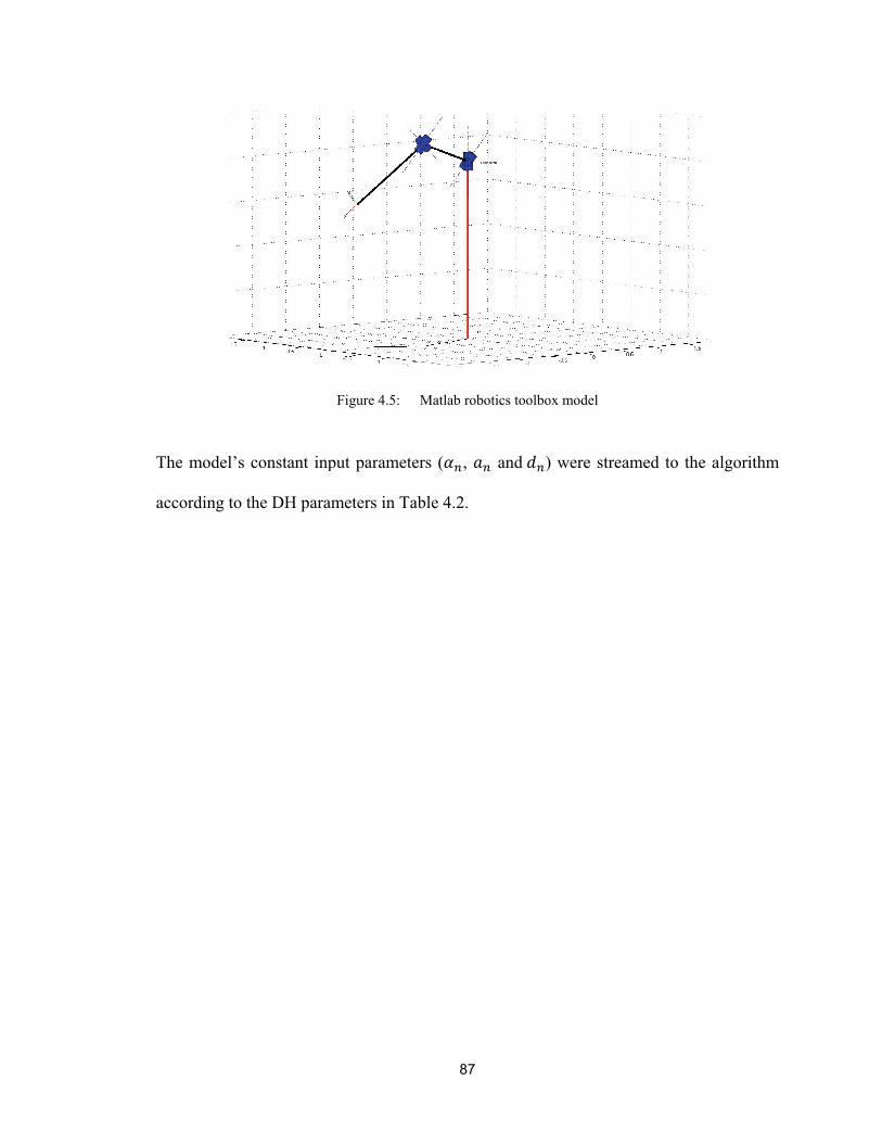
T

ac

The model’s

ccording to t

constant inp

the DH para

put paramete

ameters in Ta

Figure 4.5:

87

ers ( ,

able 4.2.

Matlab robot

and ) wer

ics toolbox mo

re streamed

odel

to the algorrithm

88

4.4 Forward Kinematics using Dual Quaternions

As discussed already, quaternions are quadruples of numbers that can be used to express

rotation but not translational motion. Eduard Study and William Clifford expanded

quaternions to include translational motion by adding a second dual parameter to each

element of the quaternion [41], shown as:

(4.23)

such that the parameter is the dual operator, with 0. Also, the elements q00, q01, q02

and q03 are the dual elements of the quaternion.

A dual quaternion can also be written as a summation of a normal quaternion and a dual

one.

(4.24)

In this section, the dual quaternion notation used is shown as:

, (4.25)

such that and are the scalar and vector components of the dual quaternion having

real and dual parts themselves.

Dual numbers can also be used to represent angles between lines in three-dimensional

Euclidean space, such that:

89

(4.26)

where is the dual angle, is the angle between the orthogonally projected vector

V1 and vector V2. Also, the distance L is the common perpendicular distance between the

line vectors, as shown in Figure 4.6.

Figure 4.6: Illustration of the dual angle between two vectors

Aspragathos and Dimitros [40] compared homogenous transformations with dual

quaternions for robot kinematics. The dual quaternion method makes use of screw theory

to describe three-dimensional motion. Screw theory states that any motion trajectory can

be simplified by describing it as a rotation on the edge of a screw with a given pitch and

angle of rotation and a vector expressing the axis of rotation that the body rotates about

[42]. The Plucker coordinates can also express this process.

The application of screw theory through using dual quaternions [43] had been adapted

to fit the needs of the human arm model. The dual quaternion algorithm depends on the

generated DH table, like its DH method counterpart. However, the dual quaternion has

faster calculation speed as well as the immunity to singularities. The modified algorithm

procedure is outlined in the following steps [40]:

90

1. Assignment of the coordinate frames to the upper and forearm links (considering

the mounted inertial sensor modules axes) following the Denavit-Hartenberg’s

notation.

2. Construction of the DH table as stated previously in this Chapter.

3. Assignment of the unit vector , along the axis assigned using the previous

step (i.e. the joints’ axes of rotation). The initial condition of is at the base

frame, where i=0, resulting in:

4. Assignment of the unit vector , along the axis by the previous step – that

is along the common perpendicular between joints’ axes if they are parallel or

perpendicular to the plane they make if they intersect. The initial condition of

is at the base frame where i=0, resulting in:

,

Modifying the DH table to include the dual angles and yields:

This results in adding two columns to the DH table as shown in Table 4.3. Lu

and LF are the lengths of the upper and forearm, respectively.

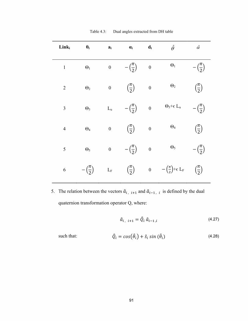
91

Table 4.3: Dual angles extracted from DH table

5. The relation between the vectors , and , is defined by the dual

quaternion transformation operator Q, where:

, , (4.27)

such that: (4.28)

Linki θi ai αi di

1 Θ1 0 2

0 Θ1 2

2 Θ2 0 2

0 Θ2 2

3 Θ3 Lu 2 0 Θ3+є Lu

2

4 Θ4 0 2

0 Θ4 2

5 Θ5 0 2

0 Θ5 2

6 2

LF 2

0 +є LF 2

92

Knowing that the cosine and sine functions for a dual angle obey the following

rules:

(4.29)

(4.30)

6. The relation between the vectors 1ˆ is and is is also defined by the Dual

quaternion transformation operator Q, where:

, (4.31)

such that , . , .

and such that . is the twist angle between the ith and the i+1 joint rotation axis.

By analogy to equations (4.29) and (4.30), the sine and cosine functions for the

dual angle , are:

, , (4.32)

, , (4.33)

7. Calculation of the position vector for forearm’s tip coordinate frame origin (also

called end- effector in robotics) is done by:

, (4.34)

93

8. Finally, the orientation of the same coordinate frame is calculated by:

, (4.35)

(4.36)

, (4.37)

Simulation results for this algorithm were produced using the CH language [44]

because of its support of the dual numbers data type and its algebra. A 5-DOF model was

designed as stated in Table 4.3, and to compare results, joint angles used were the same

as the ones used for the DH forward kinematics. Results showed that the DQ algorithm

gives an output identical to that of the DH method, with the advantage of smaller

processing times for higher degrees of freedoms as stated in [40]. The comparison

between the dual quaternion method and the DH method is summarized in Table 4.4.

94

Table 4.4: Comparison between Dual Quaternion and DH algorithms

Points of Comparison Homogenous

Transformation Dual Quaternions

Visualization of theory of operation

Easy to visualize Difficult to visualize

Quantity of Calculation

More Less

Single Rotation operation

Complex Simple

Single Translation Simple Complex

Combined rotation and translation.

Complex Simple

Gimbal Lock Problem

Might exist and cause singularities

Doesn’t Exist

A 3D position-based comparative study was made of the performances of the DH

algorithm and the Dual Quaternions one by simulating their input angles as shown in

Figure 4.7. The output 3D trajectories from both algorithms were the same, as shown in

Figure 4.8.

Figure 4.7: Input angles for comparing DH and DQ algorithms’ performance

0 10 20 30 40 50 60 70 80 90-50

-40

-30

-20

-10

0

10

20

30

40

50Input Angles (Degrees)

Sample

An

gle

(D

eg

ree

s)

Theta 1

Theta 2

Theta 3Theta 4

Theta 5

95

Figure 4.8: Simulation 3D position trajectory

Furthermore, the computing speed of the dual quaternion method showed faster results

than the DH algorithm for higher degrees of freedom systems, as shown in Figure 4.9 and

Figure 4.10.

Figure 4.9: Add/Subtract computational cost for DH vs. DQ algorithms

100

120

140

160

180

200 -150-100

-500

50100

150

-120

-100

-80

-60

-40

-20

0

20

40

60

80

Y (Millimeter)

Trajectory Comparison Between DH and DQ Algorithms

X (Millimeter)

Z (

Mill

ime

ter)

DH Algorithm Trajectory

DQ Algorithm Trajectory

0 500 1000 15000

1

2

3

4

5

6x 10

4

Degrees of Freedom

Nu

mb

er

of A

dd

ition

s a

nd

Sub

tra

ctio

ns

DH Performance

DQ Performance

96

Figure 4.10: Multiplication computational cost for DH vs. DQ algorithms

In practice, the angles were fed to the model using the estimated values acquired

from the Extended Kalman Filter after being measured using the inertial measurement

units mounted on the arm.

0 500 1000 15000

1

2

3

4

5

6

7

8

9x 10

4

Degrees of Freedom

Nu

mb

er o

f Mu

ltip

licat

ion

s

DH Performance

DQ Performance

97

4.5 Experimental Results

Proof of concept experiments have been designed for validating the local positioning

algorithms discussed in this Chapter. The experimental setup was done using the

artificial arm model and the motion tracking system mentioned in Chapter 5 section 4.

At first, a 3D motion trajectory was calculated using raw orientation angles data

from the sensors by applying directly the forward kinematics techniques. This raw

position data were considered as the measurements. After that, the angles were fed to the

EKF algorithms mentioned in Chapter 3 to obtain better position estimates after applying

forward kinematics. Local positioning results for a pitch motion trajectory are shown for

each axis separately in Figure 4.11through Figure 4.13.

Figure 4.11: EKF performance on elbow-joint positioning (x-axis)

0 10 20 30 40 50 60 70 80 90

220

240

260

280

300

320

340

Pitch Motion Trajectory X-axis Position

Time (Seconds)

Dis

tan

ce (

Mill

ime

ters

)

Measured x-axis position

Reference (Vision Tracker)EKF Output

98

Figure 4.12: EKF performance on elbow-joint positioning (y-axis)

Figure 4.13: EKF performance on elbow-joint positioning (z-axis)

Combining position data from the previous figures shows the 3D motion trajectory

shown in Figure 4.14.

10 20 30 40 50 60 70 80 90 100-200

-150

-100

-50

0

50

100

150

Pitch Motion Trajectory Y-axis Position

Time (Seconds)

Dis

tan

ce (

Mill

ime

ters

)

Measured Y-axis position

Reference (Vision Tracker)EKF Output

0 10 20 30 40 50 60 70 80 90 100-250

-200

-150

-100

-50

0

50

100

150

200

250

Pitch Motion Trajectory Z-axis Position

Time (Seconds)

Dis

tanc

e (M

illim

ete

rs)

Measured Z-axis position

Reference (Vision Tracker)EKF Output

99

Figure 4.14: EKF performance on a 3D pitch motion trajectory

Moreover, another proof of concept yaw motion trajectory was also captured and

processed like the pitch motion one mentioned earlier. The output 3D motion trajectory

proved successful comparing the reference trajectory to the estimated one as shown in

Figure 4.15.

Figure 4.15: EKF performance on a 3D yaw motion trajectory

100

Results show the performance improvement before and after applying the EKF

estimator. The position error was minimized in almost all three axes to about 5cm in each

one. Nevertheless, these error data are preliminary due to the fact that the sensors were

not perfectly synchronized, which led to time shifting and therefore maximized

subtraction errors. However, these promising results showed stability over the complete

experiment time. The preliminary error charts for all three axes are shown in Error!

Reference source not found.Figure 4.16 through Figure 4.18.

Figure 4.16: Error chart for local positioning (x-axis)

101

Figure 4.17: Error chart for local positioning (y-axis)

Figure 4.18: Error chart for local positioning (z-axis)

102

Chapter 5: EXPERIMENTAL STUDIES

The experimental design plays a significant role in the application of the proposed

monitoring system. In this Chapter, the system level designs as well as the

implementation and manufacturing phases are discussed. In general, the system is

expected to provide proof of concept as to measure and estimate human arm joint angles

and send the data wirelessly to a host PC. The host PC is responsible for performing the

more complicated mathematics on the sensor’s data being fed from the wireless sensor

modules. Finally, the testing and validation of the integrated system was done using

Matlab, CH IDE and LabVIEW programming languages.

5.1 System Design Criteria

The primary system design goal for this research is to integrate the two groups of sensors

(also called module-I and module-II) with an embedded microcontroller and a wireless

communication transceiver. To do so, some restrictions had to be specified to outline the

design methodology. The defined system criteria were defined as:

Defining the best fit from cost benefit analysis of the system components.

Low power consumption due to the need for portability.

Sufficient sampling time and processing speed for later system optimization for

real time application.

Wireless connectivity that has networking capabilities for system expansion to

model the whole human body in future research stages.

103

Small set up time of the system on the human arm to allow friendly use by

multiple patients.

The general system design is composed of two main components: the simple body

area network (BAN) containing the sensors and the host personal computer (Host PC), as

shown in Figure 5.1.

Figure 5.1: Total hardware system structural design

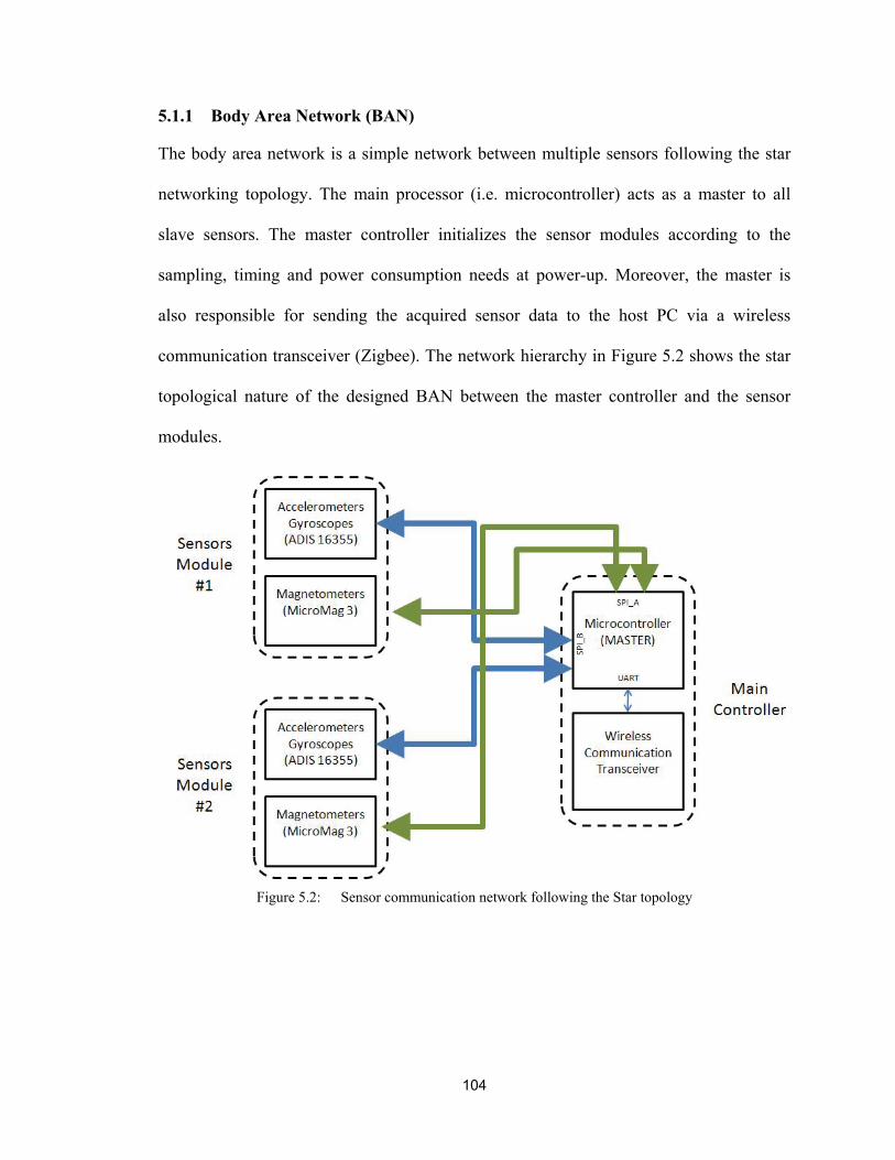
104

5.1.1 Body Area Network (BAN)

The body area network is a simple network between multiple sensors following the star

networking topology. The main processor (i.e. microcontroller) acts as a master to all

slave sensors. The master controller initializes the sensor modules according to the

sampling, timing and power consumption needs at power-up. Moreover, the master is

also responsible for sending the acquired sensor data to the host PC via a wireless

communication transceiver (Zigbee). The network hierarchy in Figure 5.2 shows the star

topological nature of the designed BAN between the master controller and the sensor

modules.

Figure 5.2: Sensor communication network following the Star topology

105

5.1.1.1 Hardware Designs

The hardware design procedure has undergone several development phases to fulfill the

needs of the project. As shown previously in Figure 5.2, the main microcontroller

communicates directly (wired) to the sensor modules. A market study of the available

inertial sensors technologies showed that digitally interfaced sensors are best for this

application, because these types of sensor include the entire necessary signal conditioning

circuitry built on-chip, dramatically reducing overall circuitry physical size. On the other

hand, the Texas Instruments MSP430F5438 microcontroller has been chosen for its low

power consumption (≈9 μ. Watts in Low-Power-Mode); furthermore, it gives some

flexibility in the hardware configuration, as will be discussed in section 5.2.2.

5.1.1.2 Sensor Module Design

Each of the two sensor modules mounted on the arm contains a complete set of triplets of

angular rate gyroscopes, accelerometers and magnetometers. The evaluation of each of

the Analog Devices ADIS16355 (Gyros and Accelerometers) as well as the PNI

MicroMag3 (Magnetometers) was done through their evaluation boards. Later, the sensor

embedded interfacing was held separately for each sensor for efficient software and

hardware debugging purposes. The ADIS16355 connection diagram for embedded

interfacing depends on the use of its many features. However, this sensor has been tested

using the Atmel AVR 8-bit MCU as well as the Texas Instruments MSP430 16-bit MCU

following the Serial Peripheral Interface (SPI) communication protocol. The ADIS16355

sensor communicates with the microcontroller through its on-chip SPI module. Similarly,

the Magnetometer (PNI Micromag3) uses the same protocol to interface with the

106

embedded controller noting the different protocol settings, as will be discussed in the

embedded software section.

However, the communication with the AVR microcontroller through the SPI

protocol was easier than with the msp430 because the ADIS16355 communication

voltage levels were the same (5V) as those of the AVR . On the other hand, the msp430

uses lower voltage levels for minimizing the power consumption (3.3V), a fact that

introduced the problem of the voltage level translation for the SPI connections. To

convert the voltage levels from one level to another, a fast switching circuit has to be

used because of the fast switching speeds on the SPI Bus – up to 2 MHz on the SPI clock.

The high-level translation was accomplished using the Maxim MAX3390, as shown in

the block diagram in Figure 5.3. The sensor connection diagram in Figure 5.3 shows the

connection dataflow used for interfacing both sensor groups to form one complete

module.

107

Due to the limitation of the input/output terminals on the level translator chip, the

data ready line for the ADIS sensor had to be sent to the controller module, maintaining

its high voltage levels (5V Logic). As a solution, another level translator was mounted on

the main controller circuitry to convert all the data-ready signals streaming in from all the

ADIS16355 sensors. The controller and communication circuits will be discussed in more

detail in the next section. The complete printed sensor circuit board 3D design was

assembled using Solid Works CAD software as shown in Figure 5.4.

Figure 5.3: Sensor module internal circuitry structure

108

The corresponding printed circuit board of the sensor model is shown in Figure 5.5.

Figure 5.5: PCB implementation of an integrated sensor module

5.1.1.3 Main Controller and Communications Module

Because of its high bit rate and full duplicity, the Serial peripheral interface (SPI)

communication protocol was used to communicate between sensors and the main

microcontroller. Data was tested using National Instrument’s LabVIEW running on a

Microsoft Windows XP platform. Although preliminary results proved successful, the

decision was made to change the controller architecture as well as the speed and power

consumption. Figure 5.6 shows the block diagram of connections used on the main

controller board. The high voltage level (5V) data ready lines extending from the

ADIS16355 modules to the controller were reduced using the voltage level translator,

also shown in Figure 5.6.

Figure 5.4: Sensor module PCB CAD model

109

The microcontroller was programmed to initialize the sensors as well as perform the

sensor calibration and filtering prior to transmitting to the host PC. First, transmitting

data wirelessly to the host PC was tested using a commercial grade off-the-shelf serial

over Bluetooth connection (BlueSmirf Gold from Sparkfun Electronics). However, this

communication method proved inconsistent because it lacked compatibility to be further

extended to cover the whole body as future work using wireless networking. Finally, the

Zigbee protocol was used to manage the wireless data communication between the BAN

and the host PC. This arrangement improved overall signal performance and filtered out

the discontinuities appearing via the Bluetooth module because of buffering problems.

Figure 5.6: Main controller modular circuit structure

110

5.1.1.4 Embedded Software Implementation

The software development for this project was split into two main categories, embedded

software and PC-based software, according to the platform type. The embedded software

was developed using IAR EW430 embedded workbench C compiler for the Texas

instruments microcontroller unit. The host PC-related software is discussed in section

5.1.2.

a. Sensors Initialization

Sensor initialization takes place at the beginning of each acquisition session at the

embedded level on the microcontroller. The initialization sequence sets the important

parameters for each sensor, such as the sampling rate, data ready interrupts, and dynamic

range. The calibration function is controlled by the host PC at this phase of the research.

Calibration is initiated by the user such that the arm should be held in a horizontal

position for some given time. Then, a graphical indicator informs the user of the end of

the calibration function. During that period, sensor data are averaged and considered as

static biases in the gyroscopes and accelerometers.

b. Communication

As stated earlier, communications on the controller module level uses standard

SPI protocol. The main concerns faced during the embedded software development

include the fact that the controller SPI packet was restricted to only 8-bits at a time,

whereas sensors used 16-bit packets. A common solution to this problem, which was

tested and verified, is to send two consecutive 8-bit packets with the chip select pin held

low as shown in Figure 5.7.

111

Figure 5.7: 16-Bit SPI word using 2x8-bit sequences

In addition to the communication with the embedded sensors, the main controller

handles the wireless communication to the host PC using Zigbee transceivers

manufactured by MaxStream, shown in Figure 5.8. This simple communication system

proved successful for a distance range of up to 30 m indoors. It can be further extended to

larger ranges using Xbee-Pro modules that support up to 90 m indoor coverage.

Figure 5.8: Wireless communication to the host PC using Zigbee™

5.1.2 Host PC System Design

The host PC system is composed of another transceiver that communicates wireless with

the BAN’s main controller. Furthermore, the data is fed to the designed PC software via a

Serial (RS232) link for further signal processing. The software program on the PC

analyzes the sensor data and estimates the orientation angles and the position of the

points of interest (i.e. elbow or wrist with respect to the shoulder’s NED frame).

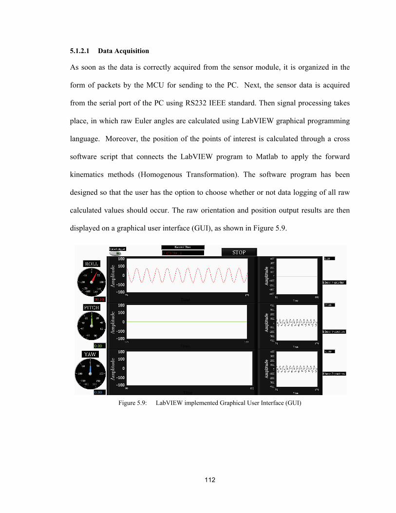
112

5.1.2.1 Data Acquisition

As soon as the data is correctly acquired from the sensor module, it is organized in the

form of packets by the MCU for sending to the PC. Next, the sensor data is acquired

from the serial port of the PC using RS232 IEEE standard. Then signal processing takes

place, in which raw Euler angles are calculated using LabVIEW graphical programming

language. Moreover, the position of the points of interest is calculated through a cross

software script that connects the LabVIEW program to Matlab to apply the forward

kinematics methods (Homogenous Transformation). The software program has been

designed so that the user has the option to choose whether or not data logging of all raw

calculated values should occur. The raw orientation and position output results are then

displayed on a graphical user interface (GUI), as shown in Figure 5.9.

Figure 5.9: LabVIEW implemented Graphical User Interface (GUI)

113

5.1.2.2 Signal Processing

The two EKF. algorithms elaborated upon in Chapter 3 are implemented in Matlab. The

programs load the input from the logged data acquisition sessions using the LabVIEW

environment mentioned in the previous section. The output estimated angles are saved in

a comma-delimited log file for further processing.

The forward kinematics was done by Soft Integration using the CH IDE linear

programming environment. This specific environment has been chosen for its well-

established libraries supporting both Denavit Hartenberg’s methods and dual number data

types. The original programming environment was designed by mechanical and

aeronautical engineer and Professor H. Cheng [44].

5.2 Sensor Calibration

Calibration can be defined as the process of comparing the data of the unit under test

(UUT) to a reference system to help minimize the error of the measuring device. This

section explains the calibration of the inertial sensors and the setups involved.

In static conditions, the complete system is fixed in a predefined orientation.

Then, sensor data are acquired and logged by the embedded system and the host PC for

further studies. Moreover, joint angles and the 3D position of selected points on the arm

are compared with data of the corresponding reference system.

The experiment procedure begins by fixing the sensor module in an equilibrium

state to log raw inertial sensor data, as shown in Figure 5.10. These data were used to

calculate static biases used in Chapter 2 as well as the construction of the covariance

matrices discussed in implementing the EKF. in Chapter 3. During data acquisition in this

or

ot

ea

d

m

fi

m

w

g

4

hu

rientation, a

ther hand sh

arth’s gravit

After

ecoupled or

mechanism in

ive degrees-

mentioned ab

was not taken

enerated som

. The offset

uman arm) t

angular rate m

how zero ac

ty vector.

Fi

the calibrati

rientation an

n such a wa

of-freedom

bove, as show

n into consi

me errors du

ts were then

the joints axe

measuremen

cceleration i

igure 5.10: S

ion step is co

ngles. The

ay that each

arm CAD m

wn in Figure

ideration du

uring position

n manually

es are consid

114

nts are zero

n the x and

Sensor Module

omplete, a si

main desig

angle can b

model was d

e 5.11. The o

uring orienta

n validation

accounted f

dered coinci

in the ideal

d y axes, and

e in Equilibrium

imple mecha

n considera

e set irrelev

designed acc

offset betwe

ation validati

n of the biom

for because

de.

case. Accel

d 1 in the z

m state

anism was ne

ation was to

vant from the

cording to t

een rotation

ions. Howev

mechanical m

in the real

lerometers o

z axis becau

eeded to me

o implemen

e other angl

the specifica

axes of the j

ver, these of

model in Cha

mechanism

on the

use of

asure

nt the

es. A

ations

joints

ffsets

apter-

m (i.e.

115

Figure 5.11: Five DOF arm CAD model

The CAD design of the arm model was made in the department’s workshop using

a Laser cutting machine. Plexiglas material was chosen as the main building material so

as to avoid using iron-core parts that would affect magnetic field measurements during

data acquisition. The final model is shown in Figure 5.12.

Figure 5.12: Implemented arm model used in experimental tests

116

5.3 Orientation Validation Test Setup

For static orientation calibration, the sensor module was placed on the link joining the

shoulder’s spherical joint to the elbow joint, because the spherical joint can rotate in all

three degrees of freedom concerning orientation – roll, pitch and yaw. In order to insure

that the link is fixed at the required orientation, the reference Microstrain’s GX2 AHRS

shown in Figure 5.13 was first mounted in the correct position, and the attached screws

were tightened to fix the model in place.

Figure 5.13: Microstrain GX-2 AHRS system

Different orientation angles for each degree of freedom are shown in Figure 5.14

through Figure 5.16.

Roll angle of -450 Roll angle of 00 Roll angle of 450

Figure 5.14: Roll testing in different orientations

117

Pitch angle of -450 Pitch angle of 00 Pitch angle of 450

Figure 5.15: Pitch testing in different orientations

Yaw angle of -450 Yaw angle of 00 Yaw angle of 450

Figure 5.16: Yaw testing in different orientations

During testing of the Yaw angle, it was observed that the measurements were

greatly affected by surrounding materials containing iron or iron alloys. To emphasize

that point, the evaluation board for the tri-axial magnetic field sensor from PNI Corp. was

pointed toward north as accurately as possible, as shown in Figure 5.17. Then, yaw

measurements were also taken, given the same orientation after placing a cast iron handle

near the sensor, as shown in Figure 5.18. Furthermore, the same experiments was

repeated but after replacing the iron handle with a conventional wrist watch, as shown in

Figure 5.19, to simulate a probable situation during a rehabilitation session.

118

Figure 5.17: Heading angle without hard-iron disturbances

Figure 5.18: Heading angle with hard-iron disturbances (iron handle)

Figure 5.19: Heading angle with hard-iron disturbances (wrist watch)

119

Results showed that the heading angle was affected to nearly 120 in the case of the

iron handle and 150 in the case of the wrist watch. These results show that compensating

for magnetic disturbances is a must, a point mentioned in recommendations for future

work.

Furthermore, dynamic orientation tests had to be made to verify the performance

of the EKF algorithms discussed in Chapter 3. At first, the implemented sensor module

was mounted on top of the GX-2 reference orientation sensor as shown in Figure 5.20 to

start the acquisition, data-logging and verification of the unit under test (UUT). After

that, both sensor modules were moved randomly by hand to ensure non linearity of

orientation.

Figure 5.20: Implemented sensor mounted on reference sensor

Having different sampling rates of both modules introduced a major challenge

during comparison between their data. The solution to that problem was introduced by

having the data logging software (i.e. LabVIEW) poll the GX-2 orientation data after

each packet received by the implemented sensor module. In this case, data from both

systems was almost perfectly synchronized.

120

5.4 Position Validation Test Setup

Position validation data was produced using the biomechanical model compared with a

real-time state-of-the-art visual motion tracking system (Visualeyez from Phoenix

Technologies Inc.) seen in Figure 5.21. The vision tracking system is composed of three

cameras to perform triangulation and provide the position of active markers mounted on

the target body.

Figure 5.21: Visualeyez motion tracking system by Phoenix Technologies

The active vision system markers were first placed as shown in Figure 5.22. The

first three markers shown on the left of the picture form the coordinate reference frame

(CRF). However, since the system doesn’t allow setting real-time CRF markers unless

they are more than 10 cm apart, their position data was first logged, and then the CRF

was created before data logging.

121

Figure 5.22: Active markers placed on the arm model for position validation

During the data acquisition/logging, the sampling time synchronization problem

was faced like the one faced with the Microstrain’s GX-2 sensor. However, this problem

was partially solved by setting the vision system to start capturing data using an external

trigger and maintain a sampling rate of 17 Hz. Nevertheless, since the implemented

module sampling rate was not exactly 17 Hz, this generated some time shifting error as

can be seen in the experimental results of Chapter 4.

Dynamic motion experiments rotating about the sensor’s y-axis (i.e. pitch) and the

z-axis (i.e. yaw) were implemented as shown in Figure 5.23 and Figure 5.24. The main

goal of these motions was to log the position of the elbow marker seen mounted at the tip

of the artificial arm model in Figure 5.23 and compare it with the output of the position

calculation algorithms from the biomechanical model. A last positioning test was made to

combine 3D rotations (roll, pitch and yaw), but unfortunately it was not successful

because only one vision tracker was available at the time of experiment that lead to the

occurrence of losses of line-of-sight.

122

Figure 5.24: Yaw motion positioning validation test

Position comparison results showed that the position of the elbow given by the

vision system had slight offsets due to the placement errors of the markers forming the

reference frame. This formed misalignment errors for the position tracking. These fixed

misalignment errors were manually subtracted later from the results before comparing to

the implemented inertial sensor module.

Figure 5.23: Pitch motion positioning validation test

123

Chapter 6: CONCLUSION AND FUTURE WORK

6.1 Conclusion

In this thesis, the main objective was to characterize the human arm motion using

kinematics for rehabilitation monitoring. The approach taken towards achieving that

objective was to use a biomechanical model of the human arm accompanied with inertial

sensors to estimate joint angles and positions of points of interest on the arm. As stated

earlier, these motion parameters can be further used for comparing saved exercise

trajectories with the ones performed by the rehabilitation subjects.

To obtain the joint angles, two Extended Kalman Filters algorithms were studied

and implemented. The first EKF. sensor fusion algorithm was used to estimate Euler

angles. The corresponding experiments showed conveniently accurate results in the Roll

and Pitch angles. However, a drawback of the developed Euler angles estimator is its

high vulnerability to external magnetic interferences as well as singularities. The second

EKF. algorithm (Quaternion-based EKF) was designed to overcome the disadvantages of

the Euler-based one. Singularity problems were solved by using quaternions instead of

Euler angles to describe orientation. Furthermore, its complementary nature – it

concentrates on estimating the errors of the states not the states themselves – gave it more

immunity to external interferences.

The biomechanical model of the human arm assumes a simplified five-degrees-of-

freedom structure of the arm. Furthermore, three forward kinematics algorithms were

studied and compared to obtain the human arm’s 3D position. First, mathematical

124

simulations were performed to compare performances of the DH and the DQ algorithms.

Results showed that the dual quaternion method is faster than the DH homogenous

transformation, especially for high degrees-of-freedom systems. Finally, the joint angles

governing the model were later taken from the outputs of the EKF. estimators.

Although the yaw angle estimation showed high performance dependency on the

surrounding electromagnetic disturbances, the complete system (orientation and local

positioning) showed consistency over time. The advantage of stability of the estimated

information can exceed the importance of highly accurate systems only stable for tens of

seconds. Another notable aspect is that the objectives of the research include providing

data for comparison of 3D trajectories using Artificial Intelligence in future work, not

determination of trajectories themselves.

In addition, the proposed system algorithms and implementation can be used

efficiently for stroke rehabilitation monitoring and assessment based on the human arm

kinematic information (i.e. 3D-position, joint-angles, etc…). The system can also be

further modified to include dynamical data such as velocities and accelerations of the

given points of interest. Other advantages of the system are the relatively low total cost,

low power consumption, and portability – it is battery-powered and wireless.

125

6.2 Future Work and Recommendations

Future work planned for this research includes implementing soft and hard iron

interference compensation for the magnetometers. Such compensation is needed for

indoor environments such as clinics, hospitals, and homes, where the magnetic

interferences are generally unknown.

Extending the number of sensor nodes to cover the human body should be

researched. In this area, general human body rehabilitation can be monitored and assessed

by studying motion of any given body part at any given time. Moreover, having the

coordinate reference frame as dynamic (i.e. fixed on the body not NED frame) would

facilitate relative positioning of the points of interest in 3D space. This can be easily done

by describing position of the points with respect to a chosen frame of a sensor as shown

in Chapter 4.

Another way to contribute significantly to the rehabilitation field is introducing

the kinematics data to artificial intelligence algorithms (Neural Networks, Fuzzy Logic,

Combined Neuro-Fuzzy, etc…) for trajectory pattern recognition. This capability can be

developed to compare the results of various exercises performed by rehabilitation

subjects.

Finally, it is recommended that an interactive graphical user-friendly interface be

designed in a video-gaming theme. This development would strongly encourage

rehabilitation patients to perform their recommended exercises actively.

126

APPENDICES

127

Appendix A: ADIS 16350 Inertial Sensor Specifications

Parameter Condition Typical Value

Gyro-sensitivity 25°C, dynamic range = ±300 °/s

Sensitivity Vs Temperature at 25°C

0.07326 °/s/LSB

<1%

Gyro-Bias Bias Vs Temp. at 25°C <4%

Gyro-axis

non-orthogonality

Different from 90° ideal at 25°C ± 0.05°

Gyro-axis misalignment Relative to base plate and guide pins at 25°C

± 0.5°

Gyro-freq. response (3dB)

Bandwidth

Sensor Resonant Freq.

350 Hz

14 kHz

Accelerometer dynamic range

initial

±10 g

25 mg/LSB

Accelerometer-axis non-Orthogonality

Different from 90° ideal at 25°C ± 0.25°

Accelerometer-axis misalignment

Relative to base plate and guide pins at 25°C

± 0.5°

Accelerometer in-Run bias stability

1σ at 25°C

Velocity random walk at 25°C

0.7 mg

2 m/s/√

Accelerometer-temperature coefficient

4 mg/°C

Accelerometer -frequency response (3dB)

Bandwidth

Sensor Resonant Freq.

350 Hz

10 kHz

128

Appendix B: PNI MicroMag-3 Magnetic Sensor Specifications

Parameter Condition Typical Value

Power Consumption 3VDC <500 μA

Magnetic Field Measurement Range

± 1100 μT

± 11 Gauss

Resolution 1/Gain (μT) 0.015 μT

0.00015 Gauss

Sampling Rate 3 VDC Up to 2000 sample/sec

Linearity Error from best fit straight line at

±300 μT

1%

Sensor Frequency 3VDC, Rb=43Ω within earth’s magnetic field

175 KHz

Operating Temperature -20 to 70 C

129

REFERENCES

[1] Canadian Institute for Health Information (CIHI), "Average admission, discharge and change in total function scores of inpatient rehabilitation clients by RCG," CIHI, Canada, Tech. Rep. NSR309, 2008.

[2] A. Ramchandani, K. Carroll, R. Buenaventura, J. Douglas and Justin Liu. (2008, Wii-habilitation increases participation in therapy. Virtual Rehabilitation, 2008 pp. 69-69.

[3] P. POUND, M. BURY and S. EBRAHIM. (1997, /9/1). From apoplexy to stroke. Age Ageing 26(5), pp. 331-337. Available: http://ageing.oxfordjournals.org

[4] World Health Organization, Cerebrovascular Disorders: A Clinical and Research Classification. ,1st ed.Geneva: WHO, 1979, pp. 82.

[5] J. L. M. Christopher and D. L. Alan, "Mortality by cause for eight regions of the world: Global Burden ofDisease Study," The Lancet, vol. 349, pp. 1269, 1997.

[6] r. A. D. Geoff, F. Marc, M. Malcolm and M. D. Stephen, "Stroke," The Lancet, vol. 371, pp. 1612, 2008.

[7] L. Oujamaa, I. Relave, J. Froger, D. Mottet and J. -. Pelissier, "Rehabilitation of arm function after stroke. Literature review," Annals of Physical and Rehabilitation Medicine, vol. 52, pp. 269, 2009.

[8] G. Prange, T. Krabben, B. Molier, H. van der Kooij and M. Jannink. (2008, A low-tech virtual reality application for training of upper extremity motor function in neurorehabilitation. Virtual Rehabilitation, 2008 pp. 8-12.

[9] P. H. Wilson, J. Duckworth, N. Mumford, R. Eldridge, M. Guglielmetti, P. Thomas, D. Shum and H. Rudolph. (2007, A virtual tabletop workspace for the assessment of upper limb function in traumatic brain injury (TBI). Virtual Rehabilitation, 2007 pp. 14-19.

[10] M. S. Cameirao, S. Bermudez i Badia, E. D. Oller and P. F. M. J. Verschure. (2008, Using a multi-task adaptive VR system for upper limb rehabilitation in the acute phase of stroke. Virtual Rehabilitation, 2008 pp. 2-7.

[11] S. Attygalle, M. Duff, T. Rikakis and Jiping He. (2008, Low-cost, at-home assessment system with wii remote based motion capture. Virtual Rehabilitation, 2008 pp. 168-174.

130

[12] S. Balasubramanian, Ruihua Wei, M. Perez, B. Shepard, E. Koeneman, J. Koeneman and Jiping He. (2008, RUPERT: An exoskeleton robot for assisting rehabilitation of arm functions. Virtual Rehabilitation, 2008 pp. 163-167.

[13] B. Dellon and Y. Matsuoka. (2008, Feedback distortion to augment controllability of human limb motion. Virtual Rehabilitation, 2008 pp. 22-27.

[14] P. Pyk, D. Wille, E. Chevrier, Y. Hauser, L. Holper, I. Fatton, R. Greipl, S. Schlegel, L. Ottiger, B. Ruckriem, A. Pescatore, A. Meyer-Heim, D. Kiper and K. Eng. (2008, A paediatric interactive therapy system for arm and hand rehabilitation. Virtual Rehabilitation, 2008 pp. 127-132.

[15] H. Zhou, T. Stone, H. Hu and N. Harris. (2008, 1). Use of multiple wearable inertial sensors in upper limb motion tracking. Med. Eng. Phys. 30(1), pp. 123-133.

[16] G. Lanfermann, R. Willmann, J. Te Vrugt, A. Timmermans, E. Bongers, N. Lambert and V. Van Acht, "Philips stroke rehabilitation exerciser," in 2007,

[17] H. Junker, O. Amft, P. Lukowicz and G. Tröster. (2008, 6). Gesture spotting with body-worn inertial sensors to detect user activities. Pattern Recognit 41(6), pp. 2010-2024.

[18] D. Roetenberg, P. J. Slycke and P. H. Veltink. (2007, Ambulatory position and orientation tracking fusing magnetic and inertial sensing. Biomedical Engineering, IEEE Transactions on 54; 54(5), pp. 883-890.

[19] H. Zheng, N. Black and N. Harris. (2005, 08/28). Position-sensing technologies for movement analysis in stroke rehabilitation. Medical and Biological Engineering and Computing 43(4), pp. 413-420. Available: http://dx.doi.org/10.1007/BF02344720

[20] E. Foxlin, "Motion tracking requirements and technologies," in Handbook of Virtual Environment Technology ,1st ed., vol. 1, K. Stanney, Ed. Lawrence Erlbaum Associates, CRC Press, 2002, pp. 163.

[21] Crossbow Technologies, "Theory of operation of angular rate sensors (application note)," Crossbow Technologies,

[22] J. Geen and D. Krakauer, "New iMEMS Angular-Rate-Sensing Gyroscope," Analog Devices Dialogue, vol. 37, pp. 12, March 2003. 2003.

[23] Analog Devices. (2008, February, 2008). ADIS16350/ADIS16355 high precision tri-axis inertial sensor data sheet (rev. A). ADI, Available: http://www.analog.com/static/imported-files/data_sheets/ADIS16350_16355.pdf

131

[24] D. Simon, "Non linear kalman filtering," in Optimal State Estimation Kalman, H-Infinity and Nonlinear Approaches ,1st edition ed., vol. 1, Anonymous USA: Wiley-Interscience, 2006, pp. 395.

[25] H. Weinberg. (1999, Dual axis, low g, Fully integrated accelerometers. Analog Devices,

[26] B. L. Stevens and F. L. Lewis, Aircraft Control and Simulation. ,2nd ed.USA: Wiley-Interscience, 2003, pp. 680.

[27] E. Bekir, Introduction to Modern Navigation Systems. Singapore: World Scientific Publishing Company, 2007, pp. 256.

[28] PNI Corp., "PNI-11096 3-axis magneto-inductive sensor driver and controller with SPI serial interface," PNI Corp., Tech. Rep. 07, February, 2003, 2003.

[29] D. Gebre-Egziabher, G. H. Elkaim, J. D. Powell and B. W. Parkinson. (2000, A gyro-free quaternion-based attitude determination system suitable for implementation using low cost sensors. Position Location and Navigation Symposium, IEEE 2000 pp. 185-192.

[30] A. J. Hanson, Visualizing Quaternions. ,1st ed., vol. 1, Canada, US: Morgan Kaufmann, 2006, pp. 600.

[31] A. M. Sabatini. (2006, Quaternion-based extended kalman filter for determining orientation by inertial and magnetic sensing. Biomedical Engineering, IEEE Transactions on 53; 53(7), pp. 1346-1356.

[32] D. Roetenberg, H. J. Luinge, C. T. M. Baten and P. H. Veltink. (2005, Compensation of magnetic disturbances improves inertial and magnetic sensing of human body segment orientation. Neural Systems and Rehabilitation Engineering, IEEE Transactions on 13; 13(3), pp. 395-405.

[33] H. Arisawa, T. Sato and T. Tomii. (2002, Human-body motion simulation using bone-based human model and construction of motion database. Conceptual Modeling for New Information Systems Technologies pp. 115-126. Available: http://dx.doi.org/10.1007/3-540-46140-X_10

[34] T. Harada, T. Gyota, Y. Kuniyoshi and T. Sato. (2007, Development of wireless networked tiny orientation device for wearable motion capture and measurement of walking around, walking up and down, and jumping tasks. Intelligent Robots and Systems, 2007. IROS 2007. IEEE/RSJ International Conference on pp. 4135-4140.

132

[35] S. Kurata, M. Makikawa, H. Kobayashi, A. Takahashi and R. Tokue. (1998, Joint motion monitoring by accelerometers set at both near sides around the joint. Engineering in Medicine and Biology Society, 1998. Proceedings of the 20th Annual International Conference of the IEEE 4; 4pp. 1936-1939 vol.4.

[36] K. Abdel-Malek, Z. Mi, J. Yang and K. Nebel. (2006, Optimization-based trajectory planning of the human upper body. Robotica 24(06), pp. 683. Available: http://journals.cambridge.org/action/displayAbstract?fromPage=online&aid=534704&fulltextType=RA&fileId=S0263574706002852RD 2006

[37] M. Treiber, "Dynamic Capture of Human Arm Motion using Inertial Sensors and Kinematical Equations," 2004.

[38] J. Lenarcic and A. Umek. (1994, Simple model of human arm reachable workspace. Systems, Man and Cybernetics, IEEE Transactions on 24; 24(8), pp. 1239-1246.

[39] J. J. Craig, Introduction to Robotics: Mechanics and Control. ,3rd ed.Prentice Hall, 2004, pp. 408.

[40] N. A. Aspragathos and J. K. Dimitros. (1998, A comparative study of three methods for robot kinematics. Systems, Man, and Cybernetics, Part B: Cybernetics, IEEE Transactions on 28; 28(2), pp. 135-145.

[41] J. McCarthy, "Dual quaternions," in Introduction to Theoritical Kinematics P. Denning, Ed. The MIT Press, 1990, pp. 62.

[42] J. K. Davidson and K. H. Hunt, "Describing the screw," in Robots and Screw Theory: Applications of Kinematics and Statics to Robotics Anonymous USA: Oxford University Press, 2004, pp. 23.

[43] J. Kim and V. Kumar. (2007, 22 March 2007). Kinematics of robot manipulators via line transformations. Journal of Robotic Systems 7(4), pp. 649.

[44] H. H. Cheng. (1994, 12/01). Programming with dual numbers and its applications in mechanisms design. Engineering with Computers 10(4), pp. 212-229. Available: http://dx.doi.org/10.1007/BF01202367