A MODAL COMPARISON OF

DOMESTIC FREIGHT TRANSPORTATION EFFECTS ON THE GENERAL PUBLIC:

2001–2009

February 2012

Prepared by CENTER FOR PORTS AND WATERWAYS

TEXAS TRANSPORTATION INSTITUTE 701 NORTH POST OAK, SUITE 430

HOUSTON, TEXAS 77024-3827 NATIONAL WATERWAYS FOUNDATION

www.nationalwaterwaysfoundation.org

A MODAL COMPARISON OF DOMESTIC FREIGHT TRANSPORTATION

EFFECTS ON THE GENERAL PUBLIC: 2001–2009

FINAL REPORT

Prepared for National Waterways Foundation

by

C. James Kruse, Director, Center for Ports & Waterways Annie Protopapas, Associate Research Scientist Leslie E. Olson, Associate Research Scientist

Texas Transportation Institute The Texas A&M University System

College Station, Texas

February 2012

v

DISCLAIMER

This research was performed in cooperation with the National Waterways Foundation

(NWF). The contents of this report reflect the views of the authors, who are responsible for the

facts and the accuracy of the data presented herein. The contents do not necessarily reflect the

official view or policies of NWF. This report does not constitute a standard, specification, or

regulation.

vi

ACKNOWLEDGMENTS

This project was conducted in cooperation with the National Waterways Foundation.

The authors wish to acknowledge the involvement and direction of Mr. Matt Woodruff, a

representative of the National Waterways Foundation.

vii

TABLE OF CONTENTS Page

List of Figures viii List of Tables ix Executive Summary 1

Background ................................................................................................................................. 1 Cargo Capacity ........................................................................................................................... 1 Congestion Issues ....................................................................................................................... 2

Highway .................................................................................................................................. 2 Rail System ............................................................................................................................. 3

Emissions Issues ......................................................................................................................... 3 Energy Efficiency ....................................................................................................................... 5 Safety Impacts ............................................................................................................................. 6

Fatalities and Injuries .............................................................................................................. 6 Hazardous Materials Incidents ................................................................................................ 8

Infrastructure Impacts ............................................................................................................... 12 Pavement Deterioration ........................................................................................................ 12 Railroad Infrastructure Impacts ............................................................................................ 12

Chapter 1: Background and Significance 13 Important Assumptions and Constraints ................................................................................... 14

Chapter 2: Congestion Issues 17 Background ............................................................................................................................... 17 Highway .................................................................................................................................... 18

Data Limitations and Necessary Assumptions ..................................................................... 24 Rail System Congestion Impacts .............................................................................................. 25

Chapter 3: Emissions Issues 29 Highway .................................................................................................................................... 29 Railroad Locomotive and Marine Emissions ............................................................................ 32

Conversion of Emission Factors to Grams per Gallon ......................................................... 32 Greenhouse Gas Emissions ....................................................................................................... 34 Summary Modal Comparison ................................................................................................... 37

Chapter 4: Energy Efficiency 39 Highway .................................................................................................................................... 39

Current/Future Federal Emissions & Energy Regulations — On-Road Vehicles ................ 39 Rail ............................................................................................................................................ 40 Inland Towing ........................................................................................................................... 41

Chapter 5: Safety Impacts 47 Fatalities and Injuries ................................................................................................................ 47 Hazardous Materials Incidents .................................................................................................. 49

Chapter 6: Infrastructure Impacts 53 Pavement Deterioration ............................................................................................................ 53

Further Highway Infrastructure Impacts ............................................................................... 56 Railroad Infrastructure Impacts ................................................................................................ 57

Appendix A: Comparative Charts

viii

LIST OF FIGURES Page Figure ES-1. Modal Freight Unit Capacities. ................................................................................ 2 Figure ES-2. Cargo Capacity Examples. ....................................................................................... 2 Figure ES-3. Metric Tons of GHG per Million Ton-Miles (2005 & 2009). .................................. 5 Figure ES-4. Comparison of Fuel Efficiency—2009. ................................................................... 5 Figure ES-5. Comparison of Fuel Efficiency—2005 & 2009. ...................................................... 6 Figure ES-6. Ratio of Fatalities per Million Ton-Miles Versus Inland Towing—2001–2009. ..... 7 Figure ES-7. Ratio of Injuries per Million Ton-Miles Versus Inland Marine—2001–2009. ........ 7 Figure ES-8. Ratio of Fatalities per Million Ton-Miles Versus Inland Towing (2001–2005 &

2001–2009). ............................................................................................................................ 8 Figure ES–9. Ratio of Injuries per Million Ton-Miles versus Inland Towing (2001–2005 &

2001–2009............................................................................................................................... 8 Figure ES-10. Gallons Spilled per Million Haz-Mat Ton-Miles (2001–2009). .......................... 11 Figure ES-11. Gallons Spilled per Million Haz-Mat Ton-Miles (2001–2005 & 2001–2009). ... 11 Figure 1. 2009 Inland Waterway Barge Traffic by Commodity Group (in millions of tons). ..... 14 Figure 2. 2009 Inland Waterway Barge Traffic by Commodity Group (in millions of tons). ..... 17 Figure 3. Average Daily Vehicles per Lane of Rural Interstate vs. Intercity Truck Ton-miles. . 21 Figure 4. Average Daily Long-Haul Truck Traffic on the National Highway System (2007). ... 23 Figure 5. Peak-Period Congestion on High-Volume Truck Portions of the National Highway

System (2007). ...................................................................................................................... 24 Figure 6. Predicted CSX train velocity with addition of Ohio River coal tonnage. .................... 27 Figure 7. Nonattainment Areas in Study Area. ............................................................................ 31 Figure 8. Ton-Miles per Metric Ton of GHG—2009. ................................................................. 35 Figure 9. Metric Tons of GHG per Million Ton-Miles—2009. .................................................. 36 Figure 10. Ton-Miles/Gal Linear Trend ...................................................................................... 43 Figure 11. Comparison of Fuel Efficiency—2009. ..................................................................... 45 Figure 12. Ratio of Fatalities per Million Ton-Miles Versus Inland Marine—2001–2009. ........ 48 Figure 13. Ratio of Injuries per Million Ton-Miles Versus Inland Marine—2001–2009. .......... 49 Figure 14. Gallons Spilled per Million Haz-Mat Ton-Miles (2001–2009). ................................ 52 Figure 15. Semitrailer configuration 3-S2: the 18-wheeler. ........................................................ 53 Figure 16. CSX IN-IL-Ohio River regional railroad network. .................................................... 57

ix

LIST OF TABLES Page Table ES-1. Standard Modal Freight Unit Capacities. .................................................................. 1 Table ES-2. Summary of Emissions—Grams per Ton-Mile—2009. ............................................ 3 Table ES-3. Summary of Emissions—Grams per Ton-Mile—2005 & 2009. ............................... 4 Table ES-4. Comparison of Large Spills Across Modes—2001–2009. ...................................... 10 Table 1. Waterway and Truck Equivalents — 2009 Tonnage and Ton-miles. ............................ 18 Table 2. Intercity Truck Ton-Miles vs. Rural Interstate Vehicle Traffic. .................................... 20 Table 3. CSX Railroad Performance Measures. .......................................................................... 27 Table 4. Emissions Analysis Results—2009. .............................................................................. 30 Table 5. 2009 Conversion Factors for Emissions in g/gal of Fuel Use. ...................................... 32 Table 7. 2009 EPA Greenhouse Gas Emissions Parameters—CO2. ........................................... 34 Table 8. Summary of Emissions—Grams per Ton-Mile—2009. ................................................ 37 Table 9. Calculated Railroad Fuel Efficiency—2009. ................................................................. 41 Table 11. Marine Fuel Efficiency. ............................................................................................... 44 Table 12. Summary of Fuel Efficiency (2009). ........................................................................... 44 Table 13. Fatality Statistics by Mode—2001–2009. ................................................................... 48 Table 14. Comparison of Injuries by Mode—2001–2009. .......................................................... 49 Table 15. Comparison of Large Spills Across Modes—2001–2009. .......................................... 51

1

1

EXECUTIVE SUMMARY

BACKGROUND

This report updates the previous modal comparison study released by the Texas Transportation Institute in December 2007, with a subsequent amendment in March 2009 that included greenhouse gas emissions. The previous study used data from 2001-2005. This study includes data from 2001–2009 (2009 is the most recent year for which data are generally available for all three modes). Inland waterway traffic continues to compare favorably to the other two modes in each category of impacts. The following topical areas were covered in this research:

• Cargo capacity • Congestion • Emissions • Energy efficiency • Safety impacts • Infrastructure impacts

The analysis is predicated on the assumption that cargo will be diverted to rail or highway (truck) modes in the event of a major waterway closure. The analysis considered the possible impacts resulting from either a diversion of 100% of the current waterborne cargo to the highway mode OR a diversion of 100% of the current waterborne cargo to the rail mode. This report presents a snapshot in time in order to focus on several vital issues. The data utilized in this research are publicly available and can be independently verified and utilized to support various analyses.

CARGO CAPACITY

The “standard” capacities for the various freight units across all three modes used in this analysis are summarized in the following table.

Table ES-1. Standard Modal Freight Unit Capacities. Modal Freight Unit Standard Cargo Capacity

Highway – Truck Trailer 25 tons Rail – Bulk Car 110 tons

Barge – Dry Bulk 1,750 tons Barge – Liquid Bulk 27,500 bbl

Figure ES-1 illustrates the carrying capacities of dry and liquid cargo barges, railcars, and semi-tractor/trailers.

2

Figure ES-1. Modal Freight Unit Capacities.

It is difficult to appreciate the carrying capacity of a barge until one understands how much demand a single barge can meet. For example, a loaded covered hopper barge carrying wheat carries enough product to make almost 2.5 million loaves of bread, or the equivalent of one loaf of bread for almost every person in the state of Kansas. A loaded tank barge carrying gasoline carries enough product to satisfy the current annual gasoline demand of approximately 2,500 people. Figure ES-2 illustrates the capacities of dry and liquid cargo barges.

Figure ES-2. Cargo Capacity Examples.

CONGESTION ISSUES

Highway

The latest national waterborne commerce data published by the U.S. Army Corps of Engineers Navigation Data Center were obtained (calendar year 2009).1 The tonnage and ton-mile data for 1 U.S. Army Corps of Engineers. Navigation Data Center. Waterborne Commerce of the United States 2009.

3

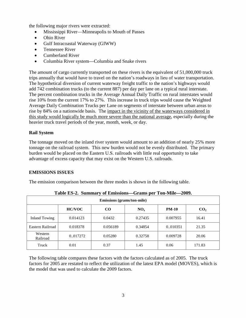
the following major rivers were extracted: • Mississippi River—Minneapolis to Mouth of Passes • Ohio River • Gulf Intracoastal Waterway (GIWW) • Tennessee River • Cumberland River • Columbia River system—Columbia and Snake rivers

The amount of cargo currently transported on these rivers is the equivalent of 51,000,000 truck trips annually that would have to travel on the nation’s roadways in lieu of water transportation. The hypothetical diversion of current waterway freight traffic to the nation’s highways would add 742 combination trucks (to the current 887) per day per lane on a typical rural interstate. The percent combination trucks in the Average Annual Daily Traffic on rural interstates would rise 10% from the current 17% to 27%. This increase in truck trips would cause the Weighted Average Daily Combination Trucks per Lane on segments of interstate between urban areas to rise by 84% on a nationwide basis. The impact in the vicinity of the waterways considered in this study would logically be much more severe than the national average, especially during the heavier truck travel periods of the year, month, week, or day.

Rail System

The tonnage moved on the inland river system would amount to an addition of nearly 25% more tonnage on the railroad system. This new burden would not be evenly distributed. The primary burden would be placed on the Eastern U.S. railroads with little real opportunity to take advantage of excess capacity that may exist on the Western U.S. railroads.

EMISSIONS ISSUES

The emission comparison between the three modes is shown in the following table.

Table ES-2. Summary of Emissions—Grams per Ton-Mile—2009. Emissions (grams/ton-mile)

HC/VOC CO NOx PM-10 CO2

Inland Towing 0.014123 0.0432 0.27435 0.007955 16.41

Eastern Railroad 0.018378 0.056189 0.34854 0..010351 21.35

Western Railroad 0..017272 0.05280 0.32758 0.009728 20.06

Truck 0.01 0.37 1.45 0.06 171.83

The following table compares these factors with the factors calculated as of 2005. The truck factors for 2005 are restated to reflect the utilization of the latest EPA model (MOVES), which is the model that was used to calculate the 2009 factors.

4

Table ES-3. Summary of Emissions—Grams per Ton-Mile—2005 & 2009. Emissions (grams/ton-mile)

Mode HC/VOC CO NOx PM CO2

2005 2009 2005 2009 2005 2009 2005 2009 2005 2009

Inland Towing 0.01737 0.014123 0.04621 0.0432 0.46907 0.27435 0.01164 0.007955 17.48 16.41

Railroad 0.02421 0.018201 0.06440 0.0556 0.65368 0.35356 0.01623 0.010251 24.39 21.14

Truck 0.12 0.10 0.46 0.37 1.90 1.45 0.08 0.06 171.87 171.83

5

Greenhouse gas emissions (GHG) expressed in metric tons of GHG produced per million ton-miles are shown in the following figure.

0

20

40

60

80

100

120

140

160

180

Inland Towing Railroads Truck Freight

16.417.48 24.38 21.13

171.87 171.83

2005 | 20092005 | 2009

2005 | 2009

Figure ES-3. Metric Tons of GHG per Million Ton-Miles (2005 & 2009).

ENERGY EFFICIENCY

Figure ES-4 presents the average fuel efficiency results in ton-miles per gallons for each of the modes on a national industry-wide basis.

0

100

200

300

400

500

600

700

Inland Towing Railroads Truck Freight

616

478

150

Figure ES-4. Comparison of Fuel Efficiency—2009.

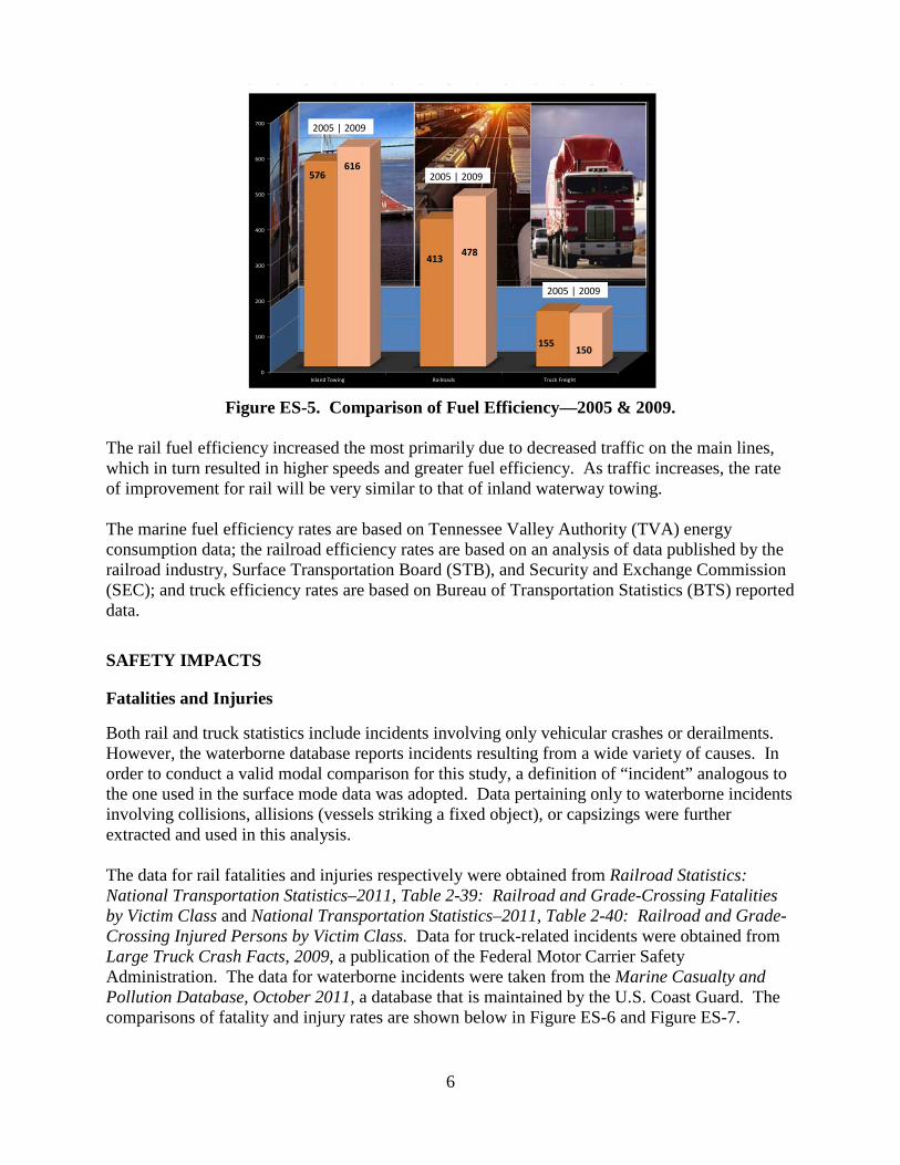
These figures have changed slightly since 2005. Figure ES-5 shows the change by mode.

6

0

100

200

300

400

500

600

700

Inland Towing Railroads Truck Freight

2005 | 2009

2005 | 2009

2005 | 2009

576616

413 478

155150

Figure ES-5. Comparison of Fuel Efficiency—2005 & 2009.

The rail fuel efficiency increased the most primarily due to decreased traffic on the main lines, which in turn resulted in higher speeds and greater fuel efficiency. As traffic increases, the rate of improvement for rail will be very similar to that of inland waterway towing. The marine fuel efficiency rates are based on Tennessee Valley Authority (TVA) energy consumption data; the railroad efficiency rates are based on an analysis of data published by the railroad industry, Surface Transportation Board (STB), and Security and Exchange Commission (SEC); and truck efficiency rates are based on Bureau of Transportation Statistics (BTS) reported data.

SAFETY IMPACTS

Fatalities and Injuries

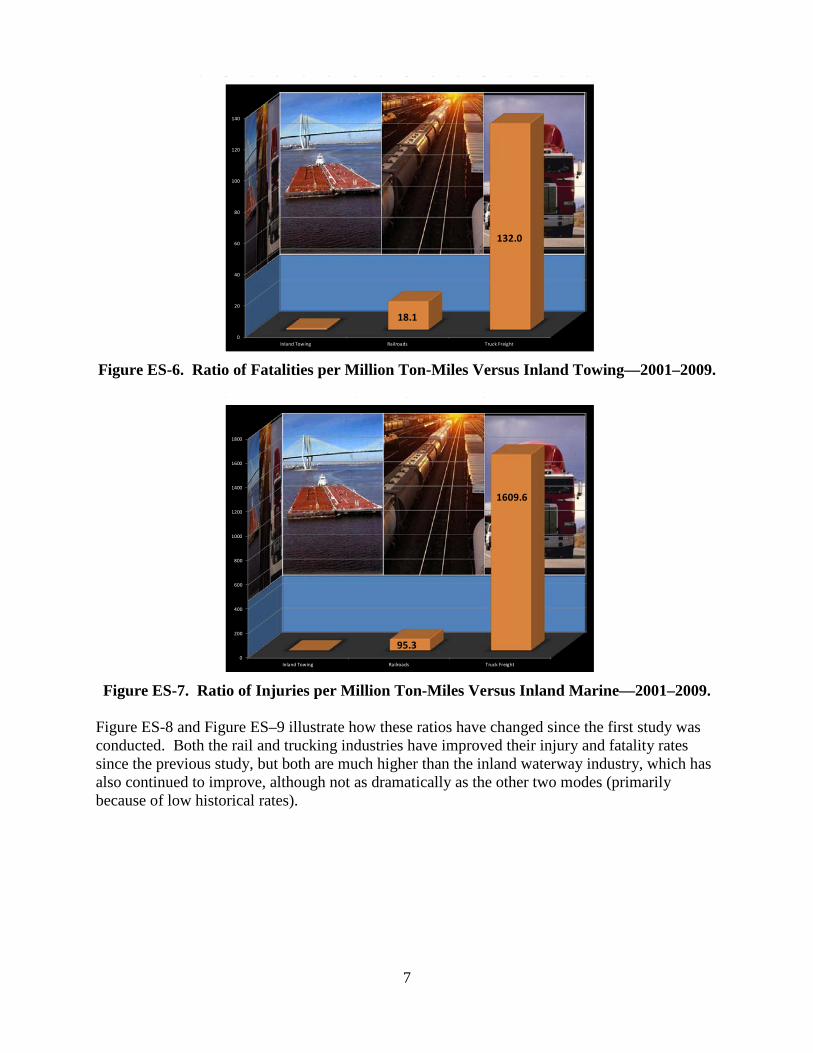
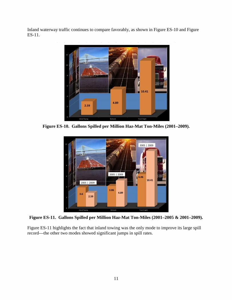
Both rail and truck statistics include incidents involving only vehicular crashes or derailments. However, the waterborne database reports incidents resulting from a wide variety of causes. In order to conduct a valid modal comparison for this study, a definition of “incident” analogous to the one used in the surface mode data was adopted. Data pertaining only to waterborne incidents involving collisions, allisions (vessels striking a fixed object), or capsizings were further extracted and used in this analysis. The data for rail fatalities and injuries respectively were obtained from Railroad Statistics: National Transportation Statistics–2011, Table 2-39: Railroad and Grade-Crossing Fatalities by Victim Class and National Transportation Statistics–2011, Table 2-40: Railroad and Grade-Crossing Injured Persons by Victim Class. Data for truck-related incidents were obtained from Large Truck Crash Facts, 2009, a publication of the Federal Motor Carrier Safety Administration. The data for waterborne incidents were taken from the Marine Casualty and Pollution Database, October 2011, a database that is maintained by the U.S. Coast Guard. The comparisons of fatality and injury rates are shown below in Figure ES-6 and Figure ES-7.

7

0

20

40

60

80

100

120

140

Inland Towing Railroads Truck Freight

18.1

132.0

Figure ES-6. Ratio of Fatalities per Million Ton-Miles Versus Inland Towing—2001–2009.

0

200

400

600

800

1000

1200

1400

1600

1800

Inland Towing Railroads Truck Freight

95.3

1609.6

Figure ES-7. Ratio of Injuries per Million Ton-Miles Versus Inland Marine—2001–2009.

Figure ES-8 and Figure ES–9 illustrate how these ratios have changed since the first study was conducted. Both the rail and trucking industries have improved their injury and fatality rates since the previous study, but both are much higher than the inland waterway industry, which has also continued to improve, although not as dramatically as the other two modes (primarily because of low historical rates).

8

0

20

40

60

80

100

120

140

160

Inland Towing Railroads Truck Freight

22.718.1

155132

2005 | 2009

2005 | 2009

2005 | 2009

Figure ES-8. Ratio of Fatalities per Million Ton-Miles Versus Inland Towing (2001–2005

& 2001–2009).

0

500

1000

1500

2000

2500

Inland Towing Railroads Truck Freight

95.3125.2

2171.5

1609.6

2005 | 20092005 | 2009

2005 | 2009

Figure ES–9. Ratio of Injuries per Million Ton-Miles versus Inland Towing (2001–2005 &

2001–2009.

Hazardous Materials Incidents

Data on hazardous materials incidents for rail and truck were taken from the Pipeline and Hazardous Materials Safety Administration’s on-line Hazmat Incident Report database. Data for inland waterway incidents were extracted from the Coast Guard’s Marine Information for Safety and Law Enforcement (MISLE) system. Due to the fact that all three reporting systems basically rely on self-reporting and the definitions of materials that require reporting are very complex, much of the spill data are suspect. However, for larger spills, it seems reasonable to assume that the accuracy of the data improves, due to the severity of the incident and public scrutiny; therefore, the research team decided to

9

analyze only large spills as a measure of the overall safety of the modes in the area of spills. The threshold quantity was set at 1,000 gallons. Table ES-4 provides a comparison of spills across the modes.

10

Table ES-4. Comparison of Large Spills Across Modes—2001–2009.

Number of Spills

Amount (gallons)

Ton-Miles (million)

Number of Spills

Amount (gallons)

Ton-Miles (million)

Number of Spills

Amount (gallons)

Ton-Miles (million)

2001 6 209,292 294,861 33 296,114 1,495,472 191 789,006 1,213,013

2002 7 32,459 293,410 29 245,183 1,507,011 153 633,534 1,245,342

2003 10 597,862 278,352 22 247,287 1,551,438 148 644,404 1,264,570

2004 11 237,155 284,096 33 379,992 1,662,598 170 4,668,493 1,281,367

2005 10 48,568 274,367 21 625,833 1,696,425 139 620,407 1,291,308

2006 8 244,800 279,778 38 671,544 1,771,897 144 551,273 1,291,244

2007 5 16,760 271,617 37 584,315 1,770,545 139 533,087 1,317,061

2008 1 1,000 260,960 18 204,248 1,777,236 119 505,043 1,131,356*

2009 1 1,000 244,995 24 427,690 1,532,214 115 475,186 1,206,025*

Total 59 1,388,896 2,482,436 255 3,682,206 14,764,836 1,318 9,420,432 11,241,286

Average 7 154,322 275,826 28 409,134 1,640,537 146 1,046,715 1,249,032

Average Annual Haz-Mat Ton-Miles (millions)

59,546 83,678* 106,847*

Rate** 0.0001101 2.5916397 0.0003386 4.8893861 0.0013706 10.411803

Ratio to Water (Inland) 3.0755973 1.8865995 12.44955 4.0174578

Mode

Year Water (Inland) Railroad Highway (Truck)

*Estimate **Spills: Spills per Million Haz-Mat Ton-Miles Amount: Gallons per Million Haz-Mat Ton-Miles

11

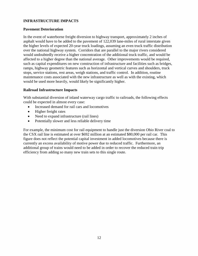
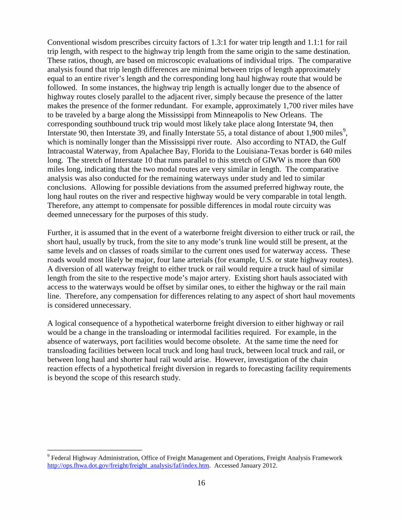
Inland waterway traffic continues to compare favorably, as shown in Figure ES-10 and Figure ES-11.

0

2

4

6

8

10

12

Inland Towing Railroads Truck Freight

2.594.89

10.41

Figure ES-10. Gallons Spilled per Million Haz-Mat Ton-Miles (2001–2009).

0

2

4

6

8

10

12

Inland Towing Railroads Truck Freight

3.63.86

6.06

4.89

10.41

2.59

2005 | 2009

2005 | 2009

2005 | 2009

Figure ES-11. Gallons Spilled per Million Haz-Mat Ton-Miles (2001–2005 & 2001–2009).

Figure ES-11 highlights the fact that inland towing was the only mode to improve its large spill record—the other two modes showed significant jumps in spill rates.

12

INFRASTRUCTURE IMPACTS

Pavement Deterioration

In the event of waterborne freight diversion to highway transport, approximately 2 inches of asphalt would have to be added to the pavement of 122,039 lane-miles of rural interstate given the higher levels of expected 20-year truck loadings, assuming an even truck traffic distribution over the national highway system. Corridors that are parallel to the major rivers considered would undoubtedly receive a higher concentration of the additional truck traffic, and would be affected to a higher degree than the national average. Other improvements would be required, such as capital expenditures on new construction of infrastructure and facilities such as bridges, ramps, highway geometric features such as horizontal and vertical curves and shoulders, truck stops, service stations, rest areas, weigh stations, and traffic control. In addition, routine maintenance costs associated with the new infrastructure as well as with the existing, which would be used more heavily, would likely be significantly higher.

Railroad Infrastructure Impacts

With substantial diversion of inland waterway cargo traffic to railroads, the following effects could be expected in almost every case:

• Increased demand for rail cars and locomotives • Higher freight rates • Need to expand infrastructure (rail lines) • Potentially slower and less reliable delivery time

For example, the minimum cost for rail equipment to handle just the diversion Ohio River coal to the CSX rail line is estimated at over $692 million at an estimated $80,000 per rail car. This figure does not reflect the potential capital investment in added locomotives because there is currently an excess availability of motive power due to reduced traffic. Furthermore, an additional group of trains would need to be added in order to recover the reduced train trip efficiency from adding so many new train sets to this single route.

13

CHAPTER 1: BACKGROUND AND SIGNIFICANCE

The Inland Waterway System (IWWS) is a key element in the nation’s transportation system. The IWWS includes approximately 12,000 miles of navigable waterways and 192 lock sites that serve navigation.2 It handles shipments to/from 38 states each year. The system is part of a larger system referred to as “America’s Marine Highways” which encompasses both deep draft and shallow draft shipping. In 20093, inland waterways maintained by the U.S. Army Corps of Engineers (Corps) handled over 522 million tons of freight (245 billion ton-miles).4 In 2007 (the most recent data available) inland waterways cargo was valued at approximately $91 billion5, resulting in an average transportation cost savings of $11/ton (as compared to other modes).6 This translates into more than $7 billion annually in transportation savings to America’s economy. Virtually all American consumers benefit from these lower transportation costs. A wide variety of public, semi-public, and private entities is involved in the maintenance and operation of the waterway. The following list illustrates the types of enterprises that directly depend on the waterways:

• Ports • Ocean-going ships • Towboats and barges • Ship-handling tugs • Marine terminals • Shipyards • Offshore supply companies • Brokers and agents • Consultants, maritime attorneys • Cruise services • Suppliers and others

The federal agencies most directly involved with the inland waterways are the Corps, the U.S. Coast Guard, and the Maritime Administration of the U.S. Department of Transportation. The Inland Waterway System is one modal network within the entire pool of domestic transportation systems networks that include truck and rail modal networks. The entire surface transportation system is becoming increasingly congested. The ability to expand this system in a timely fashion is constrained by both funding and environmental issues. Many proponents of the inland waterway system point out that it provides an effective and efficient means of expanding

2 The U.S. Waterway System — Transportation Facts, Navigation Data Center, U.S. Army Corps of Engineers,

December 2010. 3 2009 is the latest year for which data were available for all three modes. 4 Waterborne Commerce of the United States, Calendar Year 2009, Part 5–National Summaries. 5 National Transportation Statistics, 2010, Table 1-52 6 Based on data produced by the Tennessee Valley Authority using 2001 statistics.

14

capacity with less funding, has virtually unlimited capacity, and impacts the environment much less than the other modes of transportation. Figure 1 shows the composition by commodity of domestic freight tonnage transported by inland waterway barges in 2009. This figure illustrates that a very high percentage of domestic freight traffic is composed of bulk commodities—commodities that are low in value per ton and very sensitive to freight rates.

Figure 1. 2009 Inland Waterway Barge Traffic by Commodity Group (in millions of tons).

Source: Waterborne Commerce of the United States, Calendar Year 2009, Part 5—National Summaries, U.S. Army Corps of Engineers

The economics of barge transportation are easily understood and well documented. This report updates environmental, selected societal, and safety impacts of utilizing barge transportation as reported in the December 2007 report titled “A Modal Comparison of Domestic Freight Transportation Effects on the General Public” and amended in March 2009.

IMPORTANT ASSUMPTIONS AND CONSTRAINTS

The hypothetical nature of this comparative study requires certain assumptions in order to enable valid comparisons across the modes. The analysis is predicated on the assumption that cargo will be diverted to rail or highway (truck) modes in the event of a major waterway closure. The location of the closure and the alternative rail and highway routes available for bypass will determine any predominance in modal share. The geographical extent of the waterway system network does not allow any realistic predictions to be made in regards to a closure location, the alternate modal routes available for bypass, or the modal split. As a result, this analysis adopts the all-or-nothing modal assignment principle. The analysis considered the possible impacts resulting from either a theoretical diversion of 100% of

15

the current waterborne cargo to the highway mode OR a theoretical diversion of 100% of the current waterborne cargo to the rail mode. This report presents a snapshot in time in order to focus on several vital issues. The data utilized in this research are publicly available and can be independently verified and utilized to support various analyses. This analysis uses values of ton-miles of freight as the “common denominator” to enable a cross-modal comparison that takes into account both the shipment weight as well as the shipping distance. Water and rail ton-mile data are available through 2009, whereas truck ton-miles are only available through 2007. In order to provide a comparison for 2008 and 2009, the American Trucking Association’s Truck Tonnage Index for December 2008 and December 2009 was applied to the December 2007 figures. Apart from this index, four sources were used for ton-mile data: National Transportation Statistics–2011, Table 1-49: U.S. Ton-Miles of Freight (Millions); National Transportation Statistics–2011, Table 1-50, Special Tabulation (highway data); Association of American Railroads Website (2007–2009 ton-miles); and Waterborne Commerce Statistics–2009. Most of the issues related to a theoretical waterborne freight diversion are examined on a national or system-wide level. The level of detail of the available data does not permit any disaggregation, for example, to the state level. The system-wide level of analysis cannot support reasonable traffic assignment on specific highway links. It only permits a reasonable allocation of the truck traffic that would replace waterborne freight transportation to the highest class of long haul roadway, the rural segments of the interstate system. Detailed data for train fuel consumption or composition are generally proprietary; hence, not publicly available. Therefore, the research team developed methodologies for cross-referencing available train data with compiled statistics in order to support the comparative analysis among modes. Barge transportation is characterized by the longest average haul operations, followed by rail, then by truck. This study is macroscopic in nature and focuses on the main stems of the major river systems. Considerable effort took place to investigate for possible differences in route lengths (“circuity”) among the three modes, in particular between the water and highway modes. Obviously, the water and rail modes have to follow fixed routes. The highway mode is highly flexible due to the expanse of the network, but it is known that truckers have their preferred routes, and aim to minimize the total trip length, especially in longer hauls. Geographic Information Systems, using data from the National Transportation Atlas Database (NTAD)7, were used to map and compare the lengths of the major river main stems with the most logical route that would most likely be chosen by trucks transporting barge commodities from an origin at one extreme of a river to a destination at the other extreme. Educated assumptions were made about which truck routes would likely be preferred, with assistance from the Federal Highway Administration’s (FHWA) Estimated Average Annual Daily Truck Traffic8, shown in Chapter 2. 7 U.S. Department of Transportation, Research and Innovative Technology Administration, Bureau of Transportation Statistics. National Transportation Atlas Databases 2011. 8 Federal Highway Administration, Office of Highway Policy Information. Highway Statistics 2008. Section 13: Performance Indicators, System Travel Density Trends, Weighted average AADT per lane (Chart TC-201C).

16

Conventional wisdom prescribes circuity factors of 1.3:1 for water trip length and 1.1:1 for rail trip length, with respect to the highway trip length from the same origin to the same destination. These ratios, though, are based on microscopic evaluations of individual trips. The comparative analysis found that trip length differences are minimal between trips of length approximately equal to an entire river’s length and the corresponding long haul highway route that would be followed. In some instances, the highway trip length is actually longer due to the absence of highway routes closely parallel to the adjacent river, simply because the presence of the latter makes the presence of the former redundant. For example, approximately 1,700 river miles have to be traveled by a barge along the Mississippi from Minneapolis to New Orleans. The corresponding southbound truck trip would most likely take place along Interstate 94, then Interstate 90, then Interstate 39, and finally Interstate 55, a total distance of about 1,900 miles9, which is nominally longer than the Mississippi river route. Also according to NTAD, the Gulf Intracoastal Waterway, from Apalachee Bay, Florida to the Louisiana-Texas border is 640 miles long. The stretch of Interstate 10 that runs parallel to this stretch of GIWW is more than 600 miles long, indicating that the two modal routes are very similar in length. The comparative analysis was also conducted for the remaining waterways under study and led to similar conclusions. Allowing for possible deviations from the assumed preferred highway route, the long haul routes on the river and respective highway would be very comparable in total length. Therefore, any attempt to compensate for possible differences in modal route circuity was deemed unnecessary for the purposes of this study. Further, it is assumed that in the event of a waterborne freight diversion to either truck or rail, the short haul, usually by truck, from the site to any mode’s trunk line would still be present, at the same levels and on classes of roads similar to the current ones used for waterway access. These roads would most likely be major, four lane arterials (for example, U.S. or state highway routes). A diversion of all waterway freight to either truck or rail would require a truck haul of similar length from the site to the respective mode’s major artery. Existing short hauls associated with access to the waterways would be offset by similar ones, to either the highway or the rail main line. Therefore, any compensation for differences relating to any aspect of short haul movements is considered unnecessary. A logical consequence of a hypothetical waterborne freight diversion to either highway or rail would be a change in the transloading or intermodal facilities required. For example, in the absence of waterways, port facilities would become obsolete. At the same time the need for transloading facilities between local truck and long haul truck, between local truck and rail, or between long haul and shorter haul rail would arise. However, investigation of the chain reaction effects of a hypothetical freight diversion in regards to forecasting facility requirements is beyond the scope of this research study.

9 Federal Highway Administration, Office of Freight Management and Operations, Freight Analysis Framework http://ops.fhwa.dot.gov/freight/freight_analysis/faf/index.htm. Accessed January 2012.

17

CHAPTER 2: CONGESTION ISSUES

BACKGROUND

In the event of a major waterway closure, cargo will have to be diverted to either the rail or highway (truck) mode. The location of the closure and the alternative rail and highway routes available for bypass will determine any predominance in modal share. The geographical extent of the waterway system network does not allow any realistic predictions to be made in regards to a closure location, the alternate modal routes available for bypass, or the modal split. As a result, this analysis adopts the all-or-nothing modal assignment principle. The evaluation considered the possible impacts resulting from either a theoretical diversion of 100% of the current waterborne cargo to the highway mode OR a theoretical diversion of 100% of the current waterborne cargo to the rail mode. As mentioned earlier, cargoes moved on the inland waterways are typically bulk commodities with low unit values. This characteristic has a strong influence on the types of railcars and trucks that would be chosen to transport freight diverted from the waterways. The distribution by commodity groups in 2009 as shown in Figure 1 is reproduced below.

Figure 2. 2009 Inland Waterway Barge Traffic by Commodity Group (in millions of tons).

Source: Waterborne Commerce of the United States, Calendar Year 2009, Part 5—National Summaries, U.S. Army Corps of Engineers

18

HIGHWAY

Data published by the U.S. Army Corps of Engineers Navigation Data Center were obtained for calendar year 200910, the latest year for which data were available for all three modes. The domestic internal tonnage and ton-mile data for the following major rivers were extracted:

• Mississippi River—Minneapolis to Mouth of Passes • Ohio River • Gulf Intracoastal Waterway (GIWW) • Tennessee River • Cumberland River • Columbia River system—Columbia and Snake rivers

The tonnage and ton-mile data were then used to develop estimates of the equivalent truckloads, truck trips, and vehicle miles traveled that would be required if all waterway freight transported on these major rivers were to be transported by truck. All waterway data and estimated truck equivalent values are shown in Table 1. (The table assumes a cargo weight of 25 tons per truckload.) Vehicle miles traveled (vmt) is the typical unit of measure for highway travel and is simply the number of vehicles passing a point on the highway multiplied by the length of that segment of highway, measured in miles and usually on the order of one mile.

Table 1. Waterway and Truck Equivalents — 2009 Tonnage and Ton-miles.

Waterway Tonnage (x 000)

Ton-miles (x 000)

Trip Lgth

(miles)

Annual Truckloads

Annual Truck Trips

Annual Loaded

Truck vmt

Total Annual Truck vmt

Mississippi 251,931 147,151,944 584 10,077,240 20,154,480 5,886,077,760 11,772,155,520

Ohio 207,199 49,695,220 240 8,287,960 16,575,920 1,987,808,800 3,975,617,600

GIWW 107,853 16,577,116 154 4,314,120 8,628,240 663,084,640 1,326,169,280

Tennessee 39,222 4,079,154 104 1,568,880 3,137,760 163,166,160 326,332,320

Cumberland 20,824 2,149,956 103 832,960 1,665,920 85,998,240 171,996,480

Columbia/Snake 10,201 483,987 47 408,040 816,080 19,359,480 38,718,960

Total 637,230 220,137,377 — 25,489,200 50,978,400 8,805,495,080 17,610,990,160

Waterway tonnage and ton-mile data were taken from NDC. Average trip length in miles on each waterway was then calculated by division of ton-miles by miles. In reality, though, the number would denote both the average barge and truck trip length, since highway miles have been assumed to be on a 1:1 basis with river miles. Annual truckloads were calculated by dividing the tonnage for each waterway by 25 tons/truck. They were then doubled to account for an equal number of empty return trips. The truck vehicle miles traveled can be calculated in either of two ways that result in the same figure. Ton-miles can be divided by 25 tons/truck and the result doubled —to account for the empty backhaul—or the trip length can be multiplied by the annual truck trips, which has already incorporated the loaded as well as the empty return trips. 10 U.S. Army Corps of Engineers. Navigation Data Center. Waterborne Commerce of the United States 2009.

19

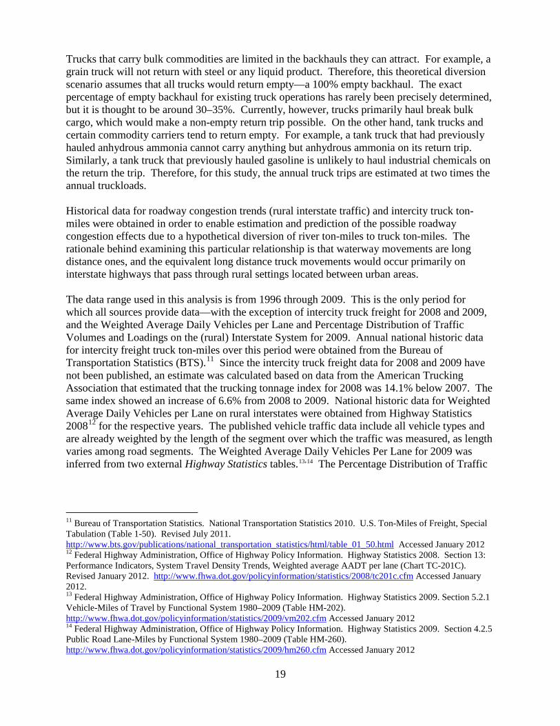
Trucks that carry bulk commodities are limited in the backhauls they can attract. For example, a grain truck will not return with steel or any liquid product. Therefore, this theoretical diversion scenario assumes that all trucks would return empty—a 100% empty backhaul. The exact percentage of empty backhaul for existing truck operations has rarely been precisely determined, but it is thought to be around 30–35%. Currently, however, trucks primarily haul break bulk cargo, which would make a non-empty return trip possible. On the other hand, tank trucks and certain commodity carriers tend to return empty. For example, a tank truck that had previously hauled anhydrous ammonia cannot carry anything but anhydrous ammonia on its return trip. Similarly, a tank truck that previously hauled gasoline is unlikely to haul industrial chemicals on the return the trip. Therefore, for this study, the annual truck trips are estimated at two times the annual truckloads. Historical data for roadway congestion trends (rural interstate traffic) and intercity truck ton-miles were obtained in order to enable estimation and prediction of the possible roadway congestion effects due to a hypothetical diversion of river ton-miles to truck ton-miles. The rationale behind examining this particular relationship is that waterway movements are long distance ones, and the equivalent long distance truck movements would occur primarily on interstate highways that pass through rural settings located between urban areas. The data range used in this analysis is from 1996 through 2009. This is the only period for which all sources provide data—with the exception of intercity truck freight for 2008 and 2009, and the Weighted Average Daily Vehicles per Lane and Percentage Distribution of Traffic Volumes and Loadings on the (rural) Interstate System for 2009. Annual national historic data for intercity freight truck ton-miles over this period were obtained from the Bureau of Transportation Statistics (BTS).11 Since the intercity truck freight data for 2008 and 2009 have not been published, an estimate was calculated based on data from the American Trucking Association that estimated that the trucking tonnage index for 2008 was 14.1% below 2007. The same index showed an increase of 6.6% from 2008 to 2009. National historic data for Weighted Average Daily Vehicles per Lane on rural interstates were obtained from Highway Statistics 200812 for the respective years. The published vehicle traffic data include all vehicle types and are already weighted by the length of the segment over which the traffic was measured, as length varies among road segments. The Weighted Average Daily Vehicles Per Lane for 2009 was inferred from two external Highway Statistics tables.13,14 The Percentage Distribution of Traffic

11 Bureau of Transportation Statistics. National Transportation Statistics 2010. U.S. Ton-Miles of Freight, Special Tabulation (Table 1-50). Revised July 2011. http://www.bts.gov/publications/national_transportation_statistics/html/table_01_50.html Accessed January 2012 12 Federal Highway Administration, Office of Highway Policy Information. Highway Statistics 2008. Section 13: Performance Indicators, System Travel Density Trends, Weighted average AADT per lane (Chart TC-201C). Revised January 2012. http://www.fhwa.dot.gov/policyinformation/statistics/2008/tc201c.cfm Accessed January 2012. 13 Federal Highway Administration, Office of Highway Policy Information. Highway Statistics 2009. Section 5.2.1 Vehicle-Miles of Travel by Functional System 1980–2009 (Table HM-202). http://www.fhwa.dot.gov/policyinformation/statistics/2009/vm202.cfm Accessed January 2012 14 Federal Highway Administration, Office of Highway Policy Information. Highway Statistics 2009. Section 4.2.5 Public Road Lane-Miles by Functional System 1980–2009 (Table HM-260). http://www.fhwa.dot.gov/policyinformation/statistics/2009/hm260.cfm Accessed January 2012

20

Volumes and Loadings on the (rural) Interstate System for 2009 was inferred from previous years’ data.15 Table 2 tabulates the data used for this analysis.

Table 2. Intercity Truck Ton-Miles vs. Rural Interstate Vehicle Traffic. Year Intercity Truck Freight

(Billion Ton-miles) Weighted Average Daily Vehicles per Lane

Rural Interstate12 1996 1,071 4,630

1997 1,119 4,788

1998 1,149 5,010

1999 1,186 5,147

2000 1,203 5,272

2001 1,224 5,381

2002 1,255 5,511

2003 1,264 5,465

2004 1,281 5,495

2005 1,291 5,439

2006 1,291 5,466

2007 1,317 5,470

2008 1,13116 5,212

2009 1,20616 5,24313,14

Linear regression techniques were then applied to the historical data to develop an equation describing the relationship between these two variables. Figure 3 shows the line fitted, the equation developed, and the R2. (R-squared, the coefficient of determination, is the proportion of variability in a data set that is accounted for by a statistical model.). The R2 is close to 1, which indicates that the line is a very good fit to the data. In other words, there is a strong relationship between values of Average Daily Vehicles per Lane on rural interstates and Intercity Truck Ton-miles, with the former historically dependent on the latter.

15 Federal Highway Administration, Office of Highway Policy Information. Highway Statistics 2008. Section 13: Performance Indicators, Percentage Distribution of Traffic Volumes and Loadings on the Interstate System (Table TC-203). Revised November 2009. http://www.fhwa.dot.gov/policyinformation/statistics/2008/tc203.cfm Accessed January 2012. 16 Estimated using ATA’s Truck Tonnage Index

21

Rural Interstate Traffic vs Intercity Truck Ton-Miles 1996-2009

y = 3.3924x + 1135.3R2 = 0.847

4,500

4,700

4,900

5,100

5,300

5,500

5,700

1,000 1,100 1,200 1,300 1,400

Intercity Truck Ton-Miles (Billions (x109))

Rur

al In

ters

tate

- W

eigh

ted

Ave

rage

Dai

ly V

ehic

les

Per L

ane

(vpl

)

Figure 3. Average Daily Vehicles per Lane of Rural Interstate vs. Intercity Truck Ton-

miles. In 2009, there were 5,243 Average Daily Vehicles per Lane on Rural Interstates, as shown in Table 2 above from Highway Statistics17 reports. Although the 2009 data are not available, it was inferred from previous year’s data that on rural interstates, in the same year, 83% of daily traffic (4,344 vehicles) was composed of passenger cars, buses, and light and heavy single unit trucks. The remaining 17% of the traffic (or 887 vehicles) was combination trucks, the types of trucks that would carry diverted waterborne freight. A total of 220.1 billion ton-miles were transported on the chosen waterways in 2009. A total of 1,206 billion ton-miles were transported by intercity trucks in 2009. If the waterway ton-miles are diverted to trucks, the new total ton-miles attributed to intercity trucks add up to 1,426 billion. When this number is input to the developed regression equation, the Weighted Average Daily Vehicles per Lane on rural interstates increases to 5,973. Since the number of passenger cars, buses, light trucks, and heavy single unit trucks are constant at 4,344 vehicles per lane, the remaining 1,629 vehicles would be combination trucks. Thus, the percentage of daily traffic that is combination trucks rises 10% from 17% to 27%. In other words, the hypothetical diversion of

17 Federal Highway Administration, Office of Highway Policy Information. Highway Statistics 2008. Section 13: Performance Indicators, Percentage Distribution of Traffic Volumes and Loadings on the Interstate System (Table TC-203). Revised November 2009. http://www.fhwa.dot.gov/policyinformation/statistics/2008/tc203.cfm Accessed January 2012.

22

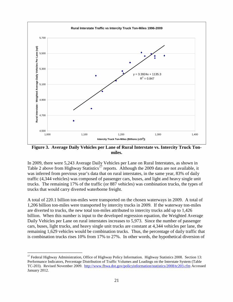
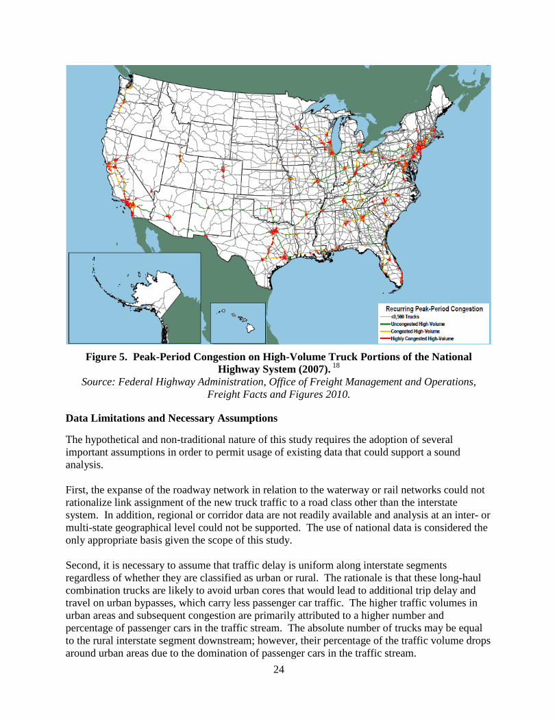
current waterway freight traffic would add 742 combination trucks (to the current 887) per day per lane on a typical rural interstate. In summary, the amount of cargo currently transported by the Mississippi main stem, Ohio main stem, Gulf Intracoastal Waterway, Tennessee River, Cumberland River, Columbia/Snake River, is the equivalent of almost 51 million truck trips annually that would have to travel on the nation’s roadways if all the tonnage currently transported by barges on these waterways were to be forced onto highways. This increase in truck trips would cause the Weighted Average Daily Combination Trucks per Lane on segments of interstate between urban areas to rise by almost 84% on a nationwide basis. This increase was derived from national level data and reflects an average nationwide increase. The absolute number and percent combination trucks per lane of rural interstate located in the vicinity of the waterways under study would likely be higher than average. Truck traffic due to the diverted waterborne freight would undoubtedly be concentrated in the corridors that are parallel to the major rivers, especially the outer lane, which tends to be used by trucks more heavily. Thus, the impact in the vicinity of the waterways considered in this study would logically be more severe than the national average, especially during the heavier truck travel periods of the year, month, week, or day. Figure 4 shows truck traffic levels on the nation’s major highways, while Figure 5 shows the locations of the major bottlenecks.

Major waterways help avoid the addition of 51 million truck trips to our highway system annually.

23

Figure 4. Average Daily Long-Haul Truck Traffic on the National Highway System

(2007).18 Source: Federal Highway Administration, Office of Freight Management and Operations,

Freight Facts and Figures 2010.

18 Source: Federal Highway Administration, Office of Freight Management and Operations, Freight Facts and Figures 2010. http://ops.fhwa.dot.gov/freight/freight_analysis/nat_freight_stats/docs/10factsfigures/index.htm Accessed January 2012.

24

Figure 5. Peak-Period Congestion on High-Volume Truck Portions of the National

Highway System (2007). 18 Source: Federal Highway Administration, Office of Freight Management and Operations,

Freight Facts and Figures 2010.

Data Limitations and Necessary Assumptions

The hypothetical and non-traditional nature of this study requires the adoption of several important assumptions in order to permit usage of existing data that could support a sound analysis. First, the expanse of the roadway network in relation to the waterway or rail networks could not rationalize link assignment of the new truck traffic to a road class other than the interstate system. In addition, regional or corridor data are not readily available and analysis at an inter- or multi-state geographical level could not be supported. The use of national data is considered the only appropriate basis given the scope of this study. Second, it is necessary to assume that traffic delay is uniform along interstate segments regardless of whether they are classified as urban or rural. The rationale is that these long-haul combination trucks are likely to avoid urban cores that would lead to additional trip delay and travel on urban bypasses, which carry less passenger car traffic. The higher traffic volumes in urban areas and subsequent congestion are primarily attributed to a higher number and percentage of passenger cars in the traffic stream. The absolute number of trucks may be equal to the rural interstate segment downstream; however, their percentage of the traffic volume drops around urban areas due to the domination of passenger cars in the traffic stream.

25

Third, it was assumed that the shorter hauls to/from interstate truck routes are of similar length and other characteristics to the existing shorter hauls to/from river segments and take place on the same road classes, which are primarily major arterials other than the interstate system. Therefore, compensation due to this issue was considered unnecessary. Finally, it was assumed that sufficient tractors, trailers, drivers, and other equipment would be available to move diverted cargo by truck. Trade journals such as the Journal of Commerce are reporting that there may be a serious shortage of truck drivers and equipment for both truck and rail movements in the near and/or long term — as it is generally accepted that freight volume growth projections will materialize once the economy sets on a steady course of recovery. Realistically, demand levels would most likely soar and, when chain reaction effects are factored in, a serious disruption to the entire supply chain could occur. However, an analysis of this type and complexity is outside the scope of this study.

RAIL SYSTEM CONGESTION IMPACTS

The intent of this rail system congestion analysis is to provide an estimate of the impact that a closure of the inland river transportation system would have on the railroad industry and the potential impact to the transportation of commodities in particular. According to the Energy Information Administration, “In 2001, railroads delivered 68.5% of coal shipments to their final electric utility destinations, followed by water (13.1 %); conveyor belts, slurry pipeline, and tramways (9.3 %); and truck (9.2 %).”19 The market for coal transportation for the railroad industry has grown rapidly in recent years. However, the downturn in the economy resulting from the recession beginning in 2008 continued to negatively affect railroad coal transportation in terms of volume. In 2009, railroads transported 10.9% fewer coal car loadings than in 2008. This analysis assumes that the market share for each transportation sector has continued to remain relatively stable since the 2001 study. 20 Data on unit and grain train velocities as well as available cars on-line were extracted from the published operating statistics as presented in the “railtimeindicators” report for January 2010 on the Association of American Railroads (AAR) website.21 The history data for cars on-line and average train velocities were obtained from both U.S. Securities and Exchange Commission (SEC) Annual 10-K Forms and Surface Transportation Board (STB) R-1 Report filings. Railroad train velocity by commodity for the Class I railroads is available on a 53-week history from the AAR website. The system velocity for all trains is reported by individual railroads in their annual reports on an inconsistent basis. In order to establish a general train speed for commodity trains the current 53-week (2011) individual railroad performance measures are used. For CSX Transportation Inc. (CSX)—the railroad used in the theoretical diversion of coal explained below—the weighted average coal train velocity for 2009 was calculated to be 17.9 miles per hour. The CSX Transportation system reported an increase of the average velocity for 19 Source: Energy Information Administration, http://www.careenergy.com/technology/transportation.asp, August 2007 20 Source: AAR website, http://www.aar.org/~/media/aar/railtimeindicators/2010-01-rti.ashx as of January 29, 2012 21 Ibid.

26

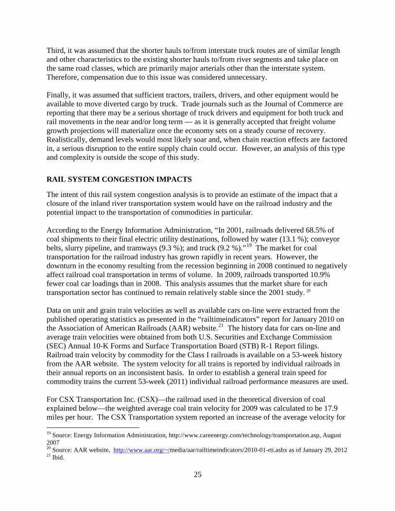
all trains year after year from 2005, 2006, and 2007. However, in 2008 CSX reported a slight decrease in average velocity for all trains. In 2009, CSX reported an increase in train velocities over 2008 of 6% as a result of reduced traffic. The 6% increase is applied to the coal train velocity assuming the same scenario holds true during 2009. The tonnage moved on the inland river system would amount to an addition of 25% more tonnage on the railroad system. This new burden would not be evenly distributed. The primary burden would be placed on the Eastern U.S. railroads with little real opportunity to take advantage of excess capacity that may exist on the Western U.S. railroads. The coal traffic on the Ohio River provides a clear example of what the effect of a major diversion of traffic would be. The Ohio River coal traffic was reported to be 118.06 million tons for the year 2009. The Ohio River (main stem) coal traffic (118.06 million short tons) represents 22.6% of the total domestic barge tonnage (522.5 million short tons) and 73% of the coal tonnage for barges for the year (161.7 million short tons). The majority of the Ohio River coal traffic would have to be handled by the CSX railroad if the Ohio River transportation system ceased operations. The CSX lines essentially parallel the Ohio River while the NS Railway lines are principally perpendicular to the river. If 118.06 million tons of Ohio River coal traffic were to be shifted to the CSX rail lines, the railroad would be faced with an additional 1,054,160 car loadings of coal annually with 112 tons of coal in each car. If the trains were made up of 108 cars per train there would be an annual addition of 9,760 train movements or 26.7 added train movements per day on the lines paralleling the Ohio River. Given the average round trip time of a unit coal train of three days, the railroad would be faced with an additional burden of at least 8,650 additional coal cars to meet this new traffic. There would be an additional 80 unit trains of 108 cars each on the Ohio River region of the CSX Railroad to meet the new traffic demand of the Ohio River coal tonnage. The CSX Railroad Annual Reports provide statistical data for average train velocity, average system dwell time, and total number of cars-on-line for the period between 2001 and 2009. The data are shown in Table 3.22 (The dwell time is the average amount of time between when a car arrives in a rail yard and when it departs the rail yard.23)

22 All data, except With Diversion column excerpted from http://investors.csx.com/phoenix.zhtml?c=92932&p=irol-reportsannual . 23 CSX Annual Report, 2003, p 10, http://media.corporate-ir.net/media_files/irol/92/92932/annual_reports/2003AR.pdf .

Diverting river traffic would add 25% more tonnage to the national rail system.

27

Table 3. CSX Railroad Performance Measures.

Figure 6. Predicted CSX train velocity with addition of Ohio River coal tonnage.

The exponential curve fit analysis indicates a poor R2 correlation coefficient of 0.3206, which implies that only the direction is predictable given the assumptions applied to the regression. Evaluating the regression equation for 2,541,160 coal car loadings provides a system average speed of 7.9 mph. Using the graphic depiction of the curve analysis above, the system average speed would be little more than 14 mph. It should be noted that the annual coal loading data and train velocities from the years 2001 to 2009 are for the entire CSX Railroad system. The actual CSX coal traffic train routes and route densities for the period between 2001 and 2009 is unknown. For the projected increased coal loadings from closing the Ohio River barge traffic, it can reasonably be assumed that the 26.6% increase in railroad coal loadings (CSX and NS combined coal loadings) will originate and terminate up or downstream in the vicinity of the Ohio River.

CSX Transportation

2001 2002 2003 2004 2005 2006 2007 2008 2009 With Diversion

Velocity All Trains 21.7 22.5 21.1 20.3 19.2 19.8 20.8 20.5 21.8 12.88

Dwell 23.2 25.3 28.7 29.7 25.6 23.2 23.3 24.1 NA

Coal car loadings (000’s) 1,722 1,574 1,570 1,659 1,726 1,798 1,771 1,779 1,487 2,541

28

Given that the added traffic would use only rail lines along the Ohio River, using the CSX System average train velocity is the best available metric to evaluate the impact on rail traffic. The increased coal traffic along the Ohio River diverted to only the CSX Railroad would increase CSX coal loadings by 41.5%. The potential for increased coal rail traffic due to closing the Ohio River transportation system would affect the local rail lines much more severely than the rest of the system. The real possibility exists that the railroad system as currently developed could not respond by accommodating the shift of coal traffic and it would either end up in gridlock or very little additional coal traffic could be accommodated.

29

CHAPTER 3: EMISSIONS ISSUES

The first part of this chapter focuses on four primary pollutants that are tracked by the Environmental Protection Agency: hydrocarbons, carbon monoxide, nitrogen oxide, and particulate matter. An analysis of greenhouse gas (GHG) emissions is included at the end of this chapter.

HIGHWAY

Emission models have been used by the Environmental Protection Agency (EPA) to evaluate highway mobile source control strategies; by states and local and regional planning agencies to develop emission inventories and control strategies for State Implementation Plans under the Clean Air Act; by metropolitan planning organizations and state transportation departments for transportation planning and conformity analysis; by academic and industry investigators conducting research; and in developing environmental impact statements.24 EPA’s newest state-of-the-art emission modeling system MOVES25 (MOtor Vehicle Emission Simulator) estimates emissions from cars, trucks, and motorcycles incorporating new car and light truck energy and greenhouse gas rates and a number of other improvements. It covers a broad range of pollutants and allows multiple scale analysis. The current version is MOVES2010a, and EPA plans to add the capability to model non-highway mobile sources, such as non-road vehicles, aircraft, locomotives, and marine vessels in future releases. MOVES is intended for official use in State Implementation Plan (SIP) development and transportation conformity determinations as required by the Clean Air Act. EPA requires the use of MOVES in new regional emissions analyses for transportation conformity determinations. Emission factor estimates depend on various conditions, such as ambient temperatures, altitude, travel speeds, operating modes, fuel volatility, mileage accrual rates, and others. Many of the variables affecting vehicle emissions can be specified by the user. The model allows modeling of specific, tailored situations via user-defined inputs that complement the basic emission factors (for example, a specific vehicle category, roadway type, time of day, etc.). MOVES2010a was utilized to model the emissions of long haul diesel fueled combination trucks nationally, based primarily on the model’s built-in default values that were derived from national fleet and vehicle activity data. The user-defined inputs used in MOVES include the following:

• Scale: national inventory • Time Span: 2009; 12 months, 7 days, 24 hours

24 International measurement standards apply to emissions mass; therefore, the unit of mass measure is grams (i.e., kilograms, and metric tons.) 25 U.S. Environmental Protection Agency, Office of Transportation and Air Quality. Motor Vehicle Emission Simulator (MOVES). http://www.epa.gov/otaq/models/moves/ Accessed January 2012.

30

• Geographic Bounds: nation • Vehicles/Equipment: diesel fuel combination long haul truck • Road Type: all (rural & urban; restricted & unrestricted access; off-network) • Pollutants:

• Volatile Organic Compounds (VOC) • Carbon Monoxide (CO) • Nitrogen Oxides (NOx) • Carbon Dioxide (CO2) • Particulate Matter of diameter 10 micrometers or less (PM-10)

• Processes: • Running/Start/Extended Idle Emissions Exhaust • Brake wear/Tire wear • Crankcase Running/Start/Extended Idle Exhaust • Refueling Displacement Vapor/Spillage Loss

• Output: • Mass units: grams • Distance units: miles • Activity: distance traveled

Table 4 shows the output of MOVES, i.e., the emission factors of the above pollutants, in grams per vmt. The output factors in grams per vmt, the total diversion truck vmt, and the diverted waterborne ton-miles were used to calculate emission rates in grams per ton-mile, which were then used to calculate the tons of additional annual emissions (Table 4). Every truck was assumed to return empty—or haul zero tons—so its return trip would have zero ton-miles. The conversion of vehicle-mile rates to ton-mile rates was necessary in order to enable a comparison with the water and rail modes on an equal basis. (Water and rail modes typically report and publish data using ton-miles, whereas highway data conventionally use vehicle-miles.)

Table 4. Emissions Analysis Results—2009. Units VOC CO NOx CO2 PM-10

g/vmt 1.30 4.68 18.11 2,147.9 0.76 g/ton-mi (or

tons/million ton-miles 0.10 0.37 1.45 171.83 0.06

Tons (000s) 23.0 82.5 319.0 37,827.0 13.3

Total truck vmt = 17.6 billion Total truck ton-miles = 220.1 billion

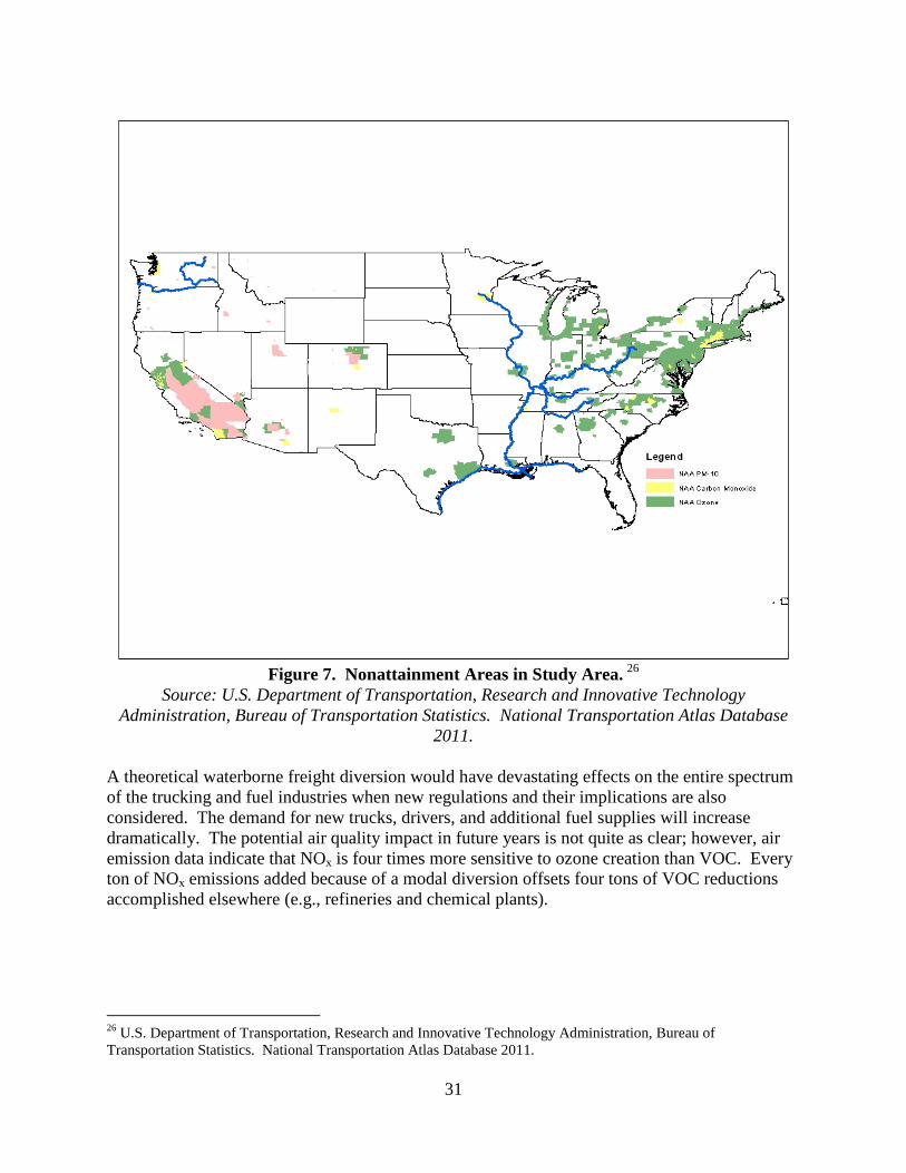
Although the range of increases in all pollutants may seem relatively modest, it must be borne in mind that the diversion truck fleet will operate primarily in the vicinity of the waterways under study. The impacts will be more severe in this geographical area than locations far away from these river bodies. The middle part of the U.S. already includes several areas designated by the EPA as Non-Attainment Areas, most commonly for ozone. The only Non-Attainment Area (for CO only) along the path of the Columbia/Snake Rivers is Portland, Oregon. Any emissions increase would only worsen existing problems. Figure 7 shows these non-attainment areas for Ozone, CO, and PM-10 nationally.

31

Figure 7. Nonattainment Areas in Study Area. 26

Source: U.S. Department of Transportation, Research and Innovative Technology Administration, Bureau of Transportation Statistics. National Transportation Atlas Database

2011. A theoretical waterborne freight diversion would have devastating effects on the entire spectrum of the trucking and fuel industries when new regulations and their implications are also considered. The demand for new trucks, drivers, and additional fuel supplies will increase dramatically. The potential air quality impact in future years is not quite as clear; however, air emission data indicate that NOx is four times more sensitive to ozone creation than VOC. Every ton of NOx emissions added because of a modal diversion offsets four tons of VOC reductions accomplished elsewhere (e.g., refineries and chemical plants).

26 U.S. Department of Transportation, Research and Innovative Technology Administration, Bureau of Transportation Statistics. National Transportation Atlas Database 2011.

32

Future Federal Regulations — On-Road Vehicles For a complete discussion of pending federal regulations, please see the section titled “Future Federal Emissions & Energy Regulations — On-Road Vehicles” in Chapter 4.

RAILROAD LOCOMOTIVE AND MARINE EMISSIONS

The emissions from railroad locomotives have been regulated by the EPA since January 1, 2001.27 During the period of this study’s “snap shot in time” of 2009, the railroads were subject to six regulated levels of emissions. The locomotive emission levels are designated as Tier 0, Tier 0+, Tier 1, Tier 1+, Tier 2, and Tier 2+ emissions.28 The regulations establish emission standards as well as methods and procedures to calculate duty-cycle emissions from locomotives.29 The EPA provides a conversion factor for the amount of pollutants locomotives would produce from each gallon of fuel used. For 2009, the EPA also provides an estimated amount of emissions for each gallon of fuel consumed—165 grams of NOx per gallon for line haul duty cycle locomotives.30

Conversion of Emission Factors to Grams per Gallon

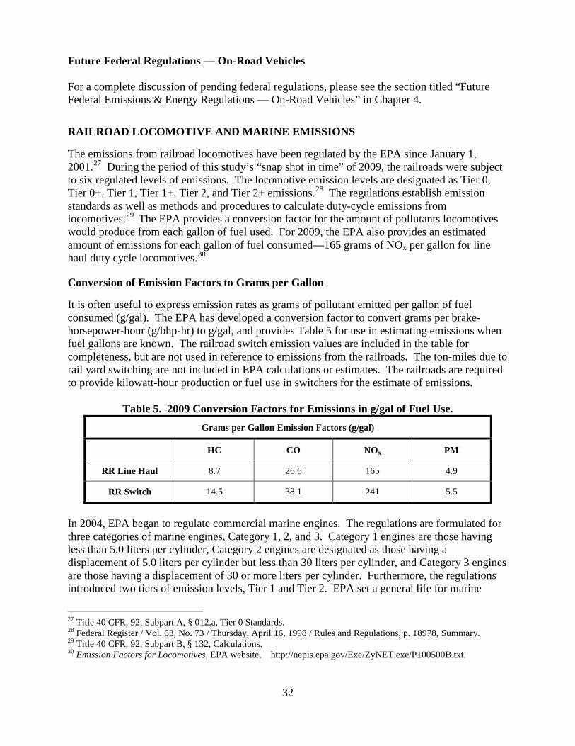
It is often useful to express emission rates as grams of pollutant emitted per gallon of fuel consumed (g/gal). The EPA has developed a conversion factor to convert grams per brake-horsepower-hour (g/bhp-hr) to g/gal, and provides Table 5 for use in estimating emissions when fuel gallons are known. The railroad switch emission values are included in the table for completeness, but are not used in reference to emissions from the railroads. The ton-miles due to rail yard switching are not included in EPA calculations or estimates. The railroads are required to provide kilowatt-hour production or fuel use in switchers for the estimate of emissions.

Table 5. 2009 Conversion Factors for Emissions in g/gal of Fuel Use. Grams per Gallon Emission Factors (g/gal)

HC CO NOx PM

RR Line Haul 8.7 26.6 165 4.9

RR Switch 14.5 38.1 241 5.5

In 2004, EPA began to regulate commercial marine engines. The regulations are formulated for three categories of marine engines, Category 1, 2, and 3. Category 1 engines are those having less than 5.0 liters per cylinder, Category 2 engines are designated as those having a displacement of 5.0 liters per cylinder but less than 30 liters per cylinder, and Category 3 engines are those having a displacement of 30 or more liters per cylinder. Furthermore, the regulations introduced two tiers of emission levels, Tier 1 and Tier 2. EPA set a general life for marine

27 Title 40 CFR, 92, Subpart A, § 012.a, Tier 0 Standards. 28 Federal Register / Vol. 63, No. 73 / Thursday, April 16, 1998 / Rules and Regulations, p. 18978, Summary. 29 Title 40 CFR, 92, Subpart B, § 132, Calculations. 30 Emission Factors for Locomotives, EPA website, http://nepis.epa.gov/Exe/ZyNET.exe/P100500B.txt.

33

engines of 10 years or 10,000 hours for Category 1 engines and 20,000 hours for Category 2 engines. Exceptions are allowed but, generally, engine manufacturers are required to petition EPA in order to obtain an exception. The 2004 regulations governing the allowable emissions for marine engines in Category 1 required only new engines or newly rebuilt engines to comply at the regulated emission levels. There was a limit with regard to the engine size and power level for the 2004 regulation, as well. For purposes of this analysis, the research team estimated the number of engines new or rebuilt in the inland waterway fleet between 2004 and 2007 (when new regulations were implemented), and determined that it was negligible and had little impact on the overall emissions output of the inland waterway fleet. In 2007, EPA introduced new requirements regarding the deadline for new engines and newly rebuilt engines to comply with Tier 2 emission limits for Category 1 and 2 engines. Beginning in the summer of 2007, new or newly rebuilt engines were required to meet new Tier 2 lower emission standards applicable for their category. Some fleet owners have taken a proactive position on complying with the emission regulations and are repowering many of their vessels with newer, higher horsepower and higher efficiency engines. Because it can be reasonably assumed that engines changed or overhauled since 2004 or 2007 must be in compliance with the governing regulations, the research team made an effort to evaluate the marine vessel fleet to determine if a reasonable estimate of the number of vessels or the amount of fleet horsepower changed since 2004 or 2007 can be made. However, the team determined that it is not reasonably possible to estimate the portion of the fleet that has become compliant with the emission regulations. In order to estimate the positive impact that emission regulation has made on the inland waterway fleet, the research team has determined an owner-by-owner examination of the fleet would be required. Beginning in 2007, EPA regulations limit commercial marine diesel engines in Category 1 to have combined total hydrocarbon/oxides of nitrogen emissions output of no more than 7.2 grams/kilowatt hour limit and Category 2 engines of between 5 and 15 liters displacement per cylinder (comparable to locomotive engines) to a combined total hydrocarbon/oxides of nitrogen emissions output of no more than 7.8 grams/kilowatt hour and particulate matter output of no more than 0.27 grams per kilowatt-hour. The revised EPA locomotive and marine emissions regulations issued in June 2008 essentially require both industries to further reduce emissions and use ultra-low sulfur diesel (ULSD). The same emission factors are used in this analysis, following the EPA intent that both commercial marine diesel engines and locomotive diesel engines be governed by the same regulation. The idle emissions for marine vessels are difficult to evaluate since every engine will idle at a different speed. Since the amount of fuel used per ton-mile of revenue is estimated based on reported fuel tax collected by the Internal Revenue Service (IRS) and the tonnage reported to the U.S. Army Corps of Engineers, the idle and running emissions are not at issue in this analysis. The same issue is present for railroad emissions with a comparable solution. Because this analysis does not attempt to develop a route specific emission profile, the idle and running emission profiles are not necessary for this study. This emission analysis uses fuel consumption by mode to estimate the emissions for that mode. Regardless of emission output per kilowatt-hour for any mode, the total fuel consumption of the

34

mode provides the total amount of emission output for that mode given that the emission per gallon of fuel consumed is equal for all modes.

GREENHOUSE GAS EMISSIONS

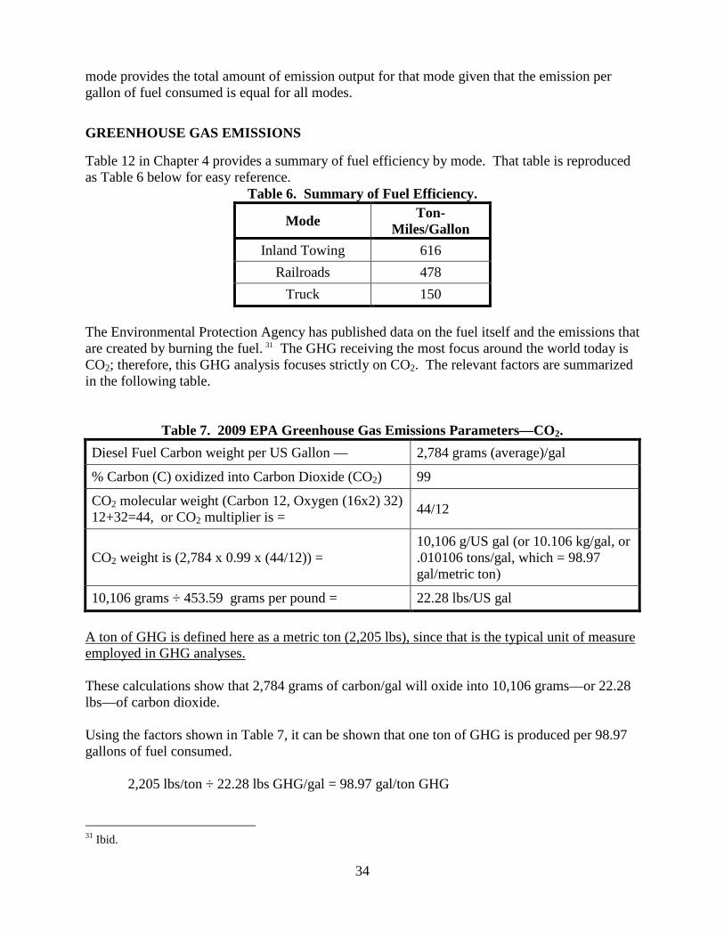
Table 12 in Chapter 4 provides a summary of fuel efficiency by mode. That table is reproduced as Table 6 below for easy reference.

Table 6. Summary of Fuel Efficiency.

Mode Ton-Miles/Gallon

Inland Towing 616 Railroads 478

Truck 150 The Environmental Protection Agency has published data on the fuel itself and the emissions that are created by burning the fuel. 31 The GHG receiving the most focus around the world today is CO2; therefore, this GHG analysis focuses strictly on CO2. The relevant factors are summarized in the following table.

Table 7. 2009 EPA Greenhouse Gas Emissions Parameters—CO2. Diesel Fuel Carbon weight per US Gallon — 2,784 grams (average)/gal

% Carbon (C) oxidized into Carbon Dioxide (CO2) 99

CO2 molecular weight (Carbon 12, Oxygen (16x2) 32) 12+32=44, or CO2 multiplier is = 44/12

CO2 weight is (2,784 x 0.99 x (44/12)) = 10,106 g/US gal (or 10.106 kg/gal, or .010106 tons/gal, which = 98.97 gal/metric ton)

10,106 grams ÷ 453.59 grams per pound = 22.28 lbs/US gal A ton of GHG is defined here as a metric ton (2,205 lbs), since that is the typical unit of measure employed in GHG analyses. These calculations show that 2,784 grams of carbon/gal will oxide into 10,106 grams—or 22.28 lbs—of carbon dioxide. Using the factors shown in Table 7, it can be shown that one ton of GHG is produced per 98.97 gallons of fuel consumed.

2,205 lbs/ton ÷ 22.28 lbs GHG/gal = 98.97 gal/ton GHG

31 Ibid.

35

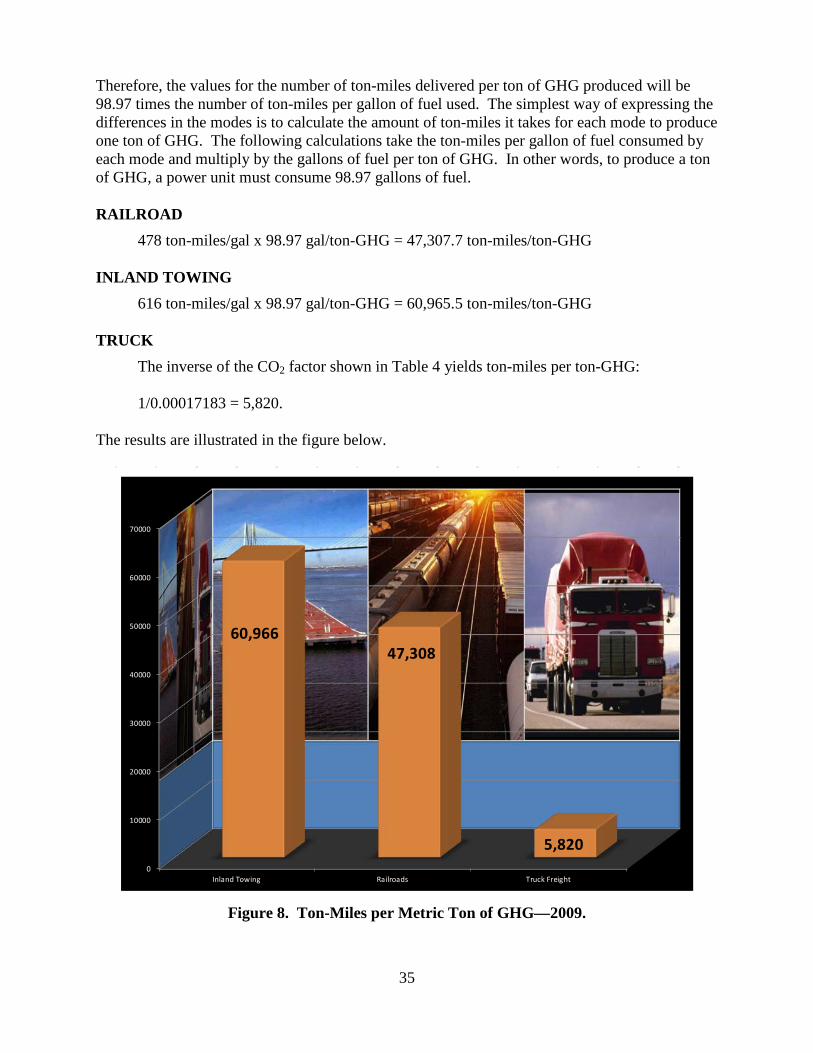
Therefore, the values for the number of ton-miles delivered per ton of GHG produced will be 98.97 times the number of ton-miles per gallon of fuel used. The simplest way of expressing the differences in the modes is to calculate the amount of ton-miles it takes for each mode to produce one ton of GHG. The following calculations take the ton-miles per gallon of fuel consumed by each mode and multiply by the gallons of fuel per ton of GHG. In other words, to produce a ton of GHG, a power unit must consume 98.97 gallons of fuel. RAILROAD 478 ton-miles/gal x 98.97 gal/ton-GHG = 47,307.7 ton-miles/ton-GHG INLAND TOWING 616 ton-miles/gal x 98.97 gal/ton-GHG = 60,965.5 ton-miles/ton-GHG TRUCK The inverse of the CO2 factor shown in Table 4 yields ton-miles per ton-GHG: 1/0.00017183 = 5,820. The results are illustrated in the figure below.

0

10000

20000

30000

40000

50000

60000

70000

Inland Towing Railroads Truck Freight

60,96647,308

5,820

Figure 8. Ton-Miles per Metric Ton of GHG—2009.

36

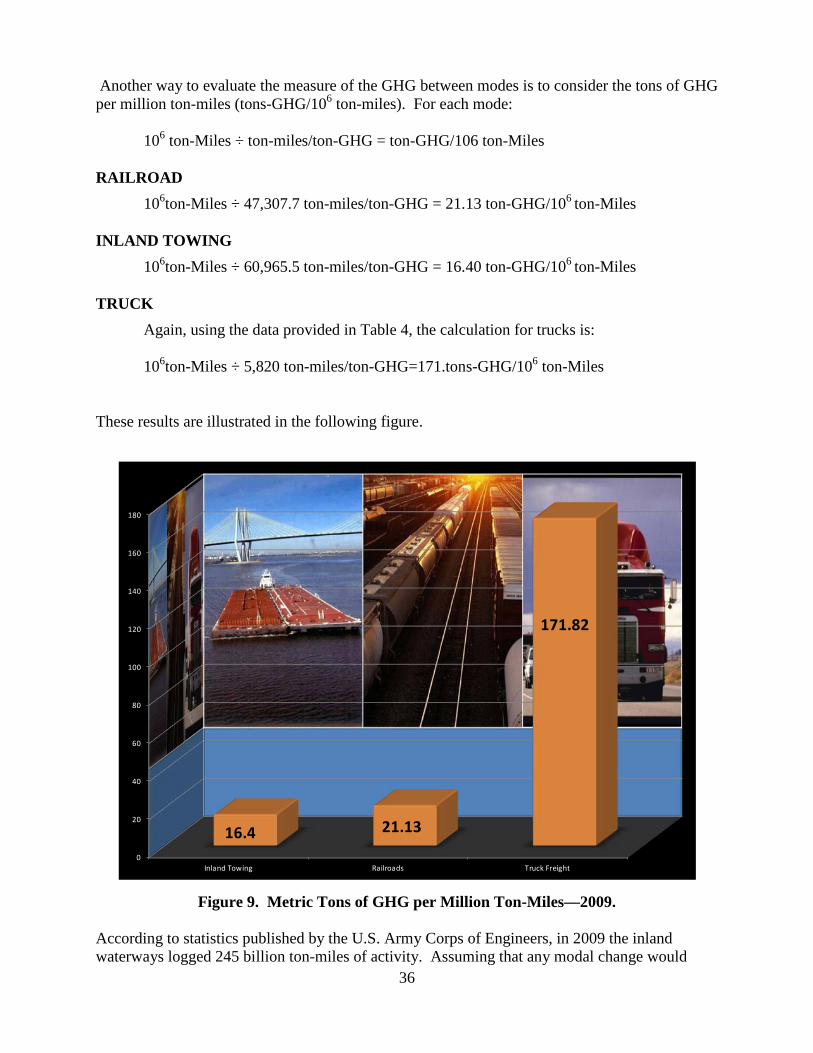
Another way to evaluate the measure of the GHG between modes is to consider the tons of GHG per million ton-miles (tons-GHG/106 ton-miles). For each mode:

106 ton-Miles ÷ ton-miles/ton-GHG = ton-GHG/106 ton-Miles RAILROAD 106ton-Miles ÷ 47,307.7 ton-miles/ton-GHG = 21.13 ton-GHG/106 ton-Miles INLAND TOWING 106ton-Miles ÷ 60,965.5 ton-miles/ton-GHG = 16.40 ton-GHG/106 ton-Miles TRUCK Again, using the data provided in Table 4, the calculation for trucks is: 106ton-Miles ÷ 5,820 ton-miles/ton-GHG=171.tons-GHG/106 ton-Miles These results are illustrated in the following figure.

0

20

40

60

80

100

120

140

160

180

Inland Towing Railroads Truck Freight

16.4 21.13

171.82

Figure 9. Metric Tons of GHG per Million Ton-Miles—2009.

According to statistics published by the U.S. Army Corps of Engineers, in 2009 the inland waterways logged 245 billion ton-miles of activity. Assuming that any modal change would

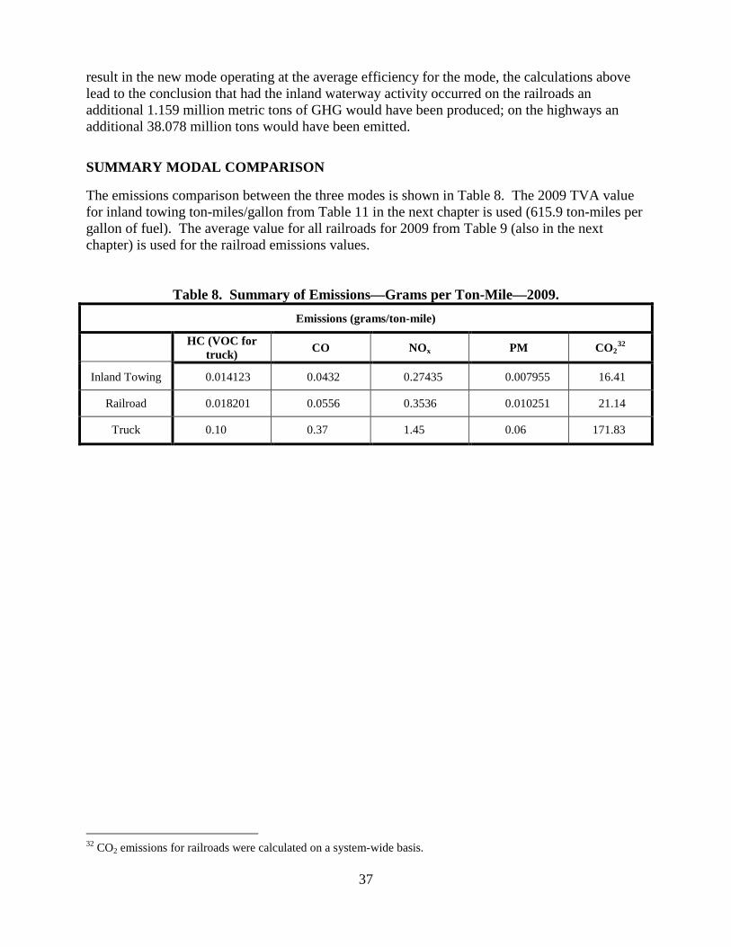
37

result in the new mode operating at the average efficiency for the mode, the calculations above lead to the conclusion that had the inland waterway activity occurred on the railroads an additional 1.159 million metric tons of GHG would have been produced; on the highways an additional 38.078 million tons would have been emitted.

SUMMARY MODAL COMPARISON

The emissions comparison between the three modes is shown in Table 8. The 2009 TVA value for inland towing ton-miles/gallon from Table 11 in the next chapter is used (615.9 ton-miles per gallon of fuel). The average value for all railroads for 2009 from Table 9 (also in the next chapter) is used for the railroad emissions values.

Table 8. Summary of Emissions—Grams per Ton-Mile—2009. Emissions (grams/ton-mile)

HC (VOC for truck) CO NOx PM CO2

32

Inland Towing 0.014123 0.0432 0.27435 0.007955 16.41

Railroad 0.018201 0.0556 0.3536 0.010251 21.14

Truck 0.10 0.37 1.45 0.06 171.83

32 CO2 emissions for railroads were calculated on a system-wide basis.

39

CHAPTER 4: ENERGY EFFICIENCY

In the comparisons for the energy intensities of the freight modes evaluated in this study, energy used for moving the empty transportation equipment on return trips was taken into account. The data for each freight transportation mode were examined to ensure that the empty movement portion was accounted for in the energy per revenue ton-mile calculations.

HIGHWAY

The Bureau of Transportation Statistics indicates that the fuel economy rate for combination trucks in 2009 was 6.0 miles per gallon33, which agrees with the figure published in the U.S. Transportation Energy Data Book.34 Conventionally, vehicle-miles traveled are used in reporting and publishing data for the highway mode, whereas ton-miles are used for the water and rail modes. For this reason, comparison of the highway mode to the other two modes in this study warranted conversion of vehicle-mile rates to ton-mile rates. When the truck fuel efficiency rate of 6.0 miles per gallon is multiplied by the assumed truckload of 25 tons of cargo, a truck fuel efficiency of 150 ton-miles per gallon is generated. Each return trip is assumed to be empty — or haul zero cargo tons. The fuel efficiency of the return trip in ton-miles per gallon mathematically would equal zero, but the fuel efficiency in vehicle-miles per gallon would still equal 6.0. Since an across the board comparison of the three modes requires the use of a ton-miles per gallon rate, 150 ton-miles per gallon is the proper figure to use, which describes the fuel efficiency of a loaded truck. A comparison of energy consumption for freight movement by the various surface transportation modes has previously been attempted. The researchers investigated the possible use of such a comparison contained in the U.S. Transportation Energy Data Book, but determined that the methodology used was not appropriate. For this report, the researchers calculated energy efficiencies using detailed data supplied by each transportation industry sector to government regulatory entities.

Current/Future Federal Emissions & Energy Regulations — On-Road Vehicles

The EPA has established a comprehensive national control program to regulate the heavy-duty vehicle and its fuel as a single system. In 2000, EPA moved forward on schedule with its rule to make heavy-duty trucks and buses run cleaner, particularly with respect to NOx and PM. Beginning with the 2007 model year, the harmful pollution from heavy-duty highway vehicles was reduced by more than 90% through the use of Ultra Low Sulfur Diesel (ULSD) in combination with the use of high-efficiency diesel particulate filters (DPF), Selective Catalytic Reduction (SCR), or Exhaust Gas Recirculation (EGR). These devices are damaged by sulfur which is why the EPA also reduced the level of sulfur in highway diesel fuel by 97% in mid- 33 Bureau of Transportation Statistics. National Transportation Statistics 2010. Table 4-14: Combination Truck Fuel Consumption and Travel. April 2010. http://www.bts.gov/publications/national_transportation_statistics/html/table_04_14.html Accessed January 2012. 34 U.S. Department of Energy. Oak Ridge National Laboratory. Davis, S.C. and Diegel, S.W. Transportation Energy Data Book: Edition 30-2011. http://cta.ornl.gov/data/index.shtml Accessed January 2012.

40

2006—from 500 parts per million (ppm) in low sulfur diesel (LSD) to 15 ppm in ULSD. The phase-in was set on a percent-of-sales basis: 50% from 2007 to 2009 and 100% in 2010. The EPA’s PM emissions standards for new heavy-duty engines were set at 0.01 grams per brake-horsepower-hour (g/bhp-hr), and took full effect for diesels in the 2007 model year. The standards for NOx and non-methane hydrocarbons (NMHC) are 0.20 g/bhp-hr and 0.14 g/bhp-hr, respectively, and took effect in January 2010. The U.S. Environmental Protection Agency (EPA) and the Department of Transportation’s National Highway Traffic Safety Administration (NHTSA) announced in October 2010 a first-ever program to reduce greenhouse gas (GHG) emissions and improve fuel efficiency of medium- and heavy-duty vehicles, such as the largest pickup trucks and vans, semi-trucks, and all types and sizes of work trucks and buses in between. These vehicles make up the transportation segment’s second largest contributor to oil consumption and GHG emissions. Standards for combination trucks in Class 8 range from 118 ton-miles/gallon to 159 ton-miles/gallon. The final rule has been issued for model years 2014-2018 and EPA and NHTSA have moved on to the implementation stage by the time of this writing. The program intends to create a strong and comprehensive heavy-duty national program (the “HD National Program”), designed to address the urgent and closely intertwined challenges of dependence on oil, energy security, and global climate change. The agencies estimate that the combined standards will reduce CO2 emissions by about 270 million metric tons and save about 530 million barrels of oil over the life of vehicles built for the 2014 to 2018 model years, providing $49 billion in net program benefits. The reduced fuel use alone will enable $50 billion in fuel savings to accrue to vehicle owners, or $42 billion in net savings when considering technology costs. A second phase of regulations is planned for model years beyond 2018. In total, the combined GHG and fuel economy standards will reduce GHG emissions from the U.S. heavy-duty fleet by approximately 76 million metric tons of CO2-equivalent annually by 2030. The HD National Program is a key component of the agencies’ response to a Presidential Memorandum issued in May 2010, and has been developed with support from industry, the State of California, and environmental stakeholders.

RAIL

For freight modes, a significant portion of the energy expended is attributed to non-haul purposes. For example, almost half of the energy consumed by freight rail is not used to move freight:

• More than 30% is used for empty backhaul. • About 4% is reported lost or spilled each year. • About 4% is consumed in idling. • 10% is used by yard locomotives assembling and switching cars.35

The energy consumption in the railroad industry was carefully evaluated in order to ensure that the full energy as well as the total equipment and freight mileage movements were included.

35 A.B. Rose, Energy Intensity and Related Parameters of Selected Transportation Modes: Freight Movements, ORNL-5554 (Oak Ridge, TN: Oak Ridge National Laboratory, June 1979), pp. S-10 and 5-4.

41

The data for the railroads were spread among four primary sources: the Association of American Railroads (AAR), the Surface Transportation Board (STB), Security and Exchange Commission (SEC), and the railroads’ own annual reports to stockholders. The AAR data were found on the AAR website in the RR Industry Info, Statistics, and Performance Measures sections. Both the SEC and the STB websites provide each railroad’s required federal filings. The SEC data source is the 10-K annual report of financial status and operating data. The STB provides each railroad’s R-1 report that includes operating data, particularly the railroad’s locomotive fuel gallons on Schedule 750, line 4, and the revenue ton-miles of traffic reported on Schedule 755, line 108. The individual railroad’s average annual cost per gallon of fuel is discretionarily available in their individual annual report. Additionally, individual railroads may include the actual gallons of locomotive fuel consumed in their annual report; however, this value is not consistently reported by any of the railroads except in their STB R-1 filings. Table 9 lists the fuel efficiency calculated by the researchers using the available data from sources described above and the AAR reported value for gross ton-miles per gallon of fuel for the year 2009 as provided in the RR Statistics document on their website.

Table 9. Calculated Railroad Fuel Efficiency—2009. Gross Revenue

Ton-Miles (x106)36 Fuel Consumed

(x106)37 Ton-Miles/Gallon38

AAR (2009) 480.0

BNSF 593,573 1,198.2 495.4

CN (US) 42,724 78.0 547.7

CPR 20,360 36.1 564.0

CSX 209,249 447.0 468.5

KCS 28,599 60.6 471.9

NS 158,520 392.5 403.9

UP 479,187 990.6 483.7

Average All Railroads 1,532,212 3,203.0 478.4

INLAND TOWING

It is more difficult to develop energy consumption data for the inland waterways (river and Gulf Intracoastal Waterways) operators than for the railroad industry. The marine industry only

36 STB R-1 Annual Report, Schedule 755, Line 110: Total Gross revenue ton-miles all trains. 37 STB R-1 Annual Report, Schedule 750, Line 4: Total Fuel Consumed all trains except passenger. 38 Calculated value, Gross Revenue Ton-Miles divided by Fuel Consumed.

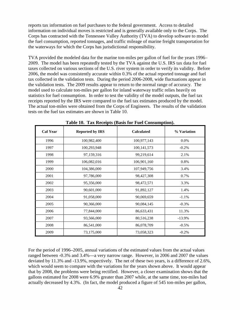
42

reports tax information on fuel purchases to the federal government. Access to detailed information on individual moves is restricted and is generally available only to the Corps. The Corps has contracted with the Tennessee Valley Authority (TVA) to develop software to model the fuel consumption, reported tonnages, and traffic mileage of marine freight transportation for the waterways for which the Corps has jurisdictional responsibility. TVA provided the modeled data for the marine ton-miles per gallon of fuel for the years 1996–2009. The model has been repeatedly tested by the TVA against the U.S. IRS tax data for fuel taxes collected on various sections of the U.S. river system in order to verify its validity. Before 2006, the model was consistently accurate within 0.3% of the actual reported tonnage and fuel tax collected in the validation tests. During the period 2006-2008, wide fluctuations appear in the validation tests. The 2009 results appear to return to the normal range of accuracy. The model used to calculate ton-miles per gallon for inland waterway traffic relies heavily on statistics for fuel consumption. In order to test the validity of the model outputs, the fuel tax receipts reported by the IRS were compared to the fuel tax estimates produced by the model. The actual ton-miles were obtained from the Corps of Engineers. The results of the validation tests on the fuel tax estimates are shown in Table 10.

Table 10. Tax Receipts (Basis for Fuel Consumption).

Cal Year Reported by IRS Calculated % Variation

1996 100,982,400 100,977,143 0.0%

1997 100,293,948 100,141,573 -0.2%

1998 97,159,316 99,219,614 2.1%

1999 106,082,016 106,901,160 0.8%

2000 104,386,000 107,949,756 3.4%

2001 97,786,000 98,427,308 0.7%

2002 95,356,000 98,472,571 3.3%

2003 90,601,000 91,892,127 1.4%

2004 91,058,000 90,069,659 -1.1%

2005 90,366,000 90,084,145 -0.3%

2006 77,844,000 86,633,431 11.3%

2007 93,566,000 80,516,238 -13.9%

2008 86,541,000 86,078,709 -0.5%

2009 73,175,000 73,058,323 -0.2%

For the period of 1996–2005, annual variations of the estimated values from the actual values ranged between -0.3% and 3.4%—a very narrow range. However, in 2006 and 2007 the values deviated by 11.3% and -13.9%, respectively. The net of these two years, is a difference of 2.6%, which would seem to compare with the variations for the years shown above. It would appear that by 2008, the problems were being rectified. However, a closer examination shows that the gallons estimated for 2008 were 6.9% greater than 2007 while, at the same time, ton-miles had actually decreased by 4.3%. (In fact, the model produced a figure of 545 ton-miles per gallon,

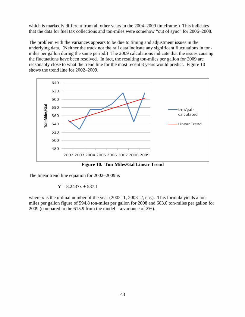
43

which is markedly different from all other years in the 2004–2009 timeframe.) This indicates that the data for fuel tax collections and ton-miles were somehow “out of sync” for 2006–2008. The problem with the variances appears to be due to timing and adjustment issues in the underlying data. (Neither the truck nor the rail data indicate any significant fluctuations in ton-miles per gallon during the same period.) The 2009 calculations indicate that the issues causing the fluctuations have been resolved. In fact, the resulting ton-miles per gallon for 2009 are reasonably close to what the trend line for the most recent 8 years would predict. Figure 10 shows the trend line for 2002–2009.

Figure 10. Ton-Miles/Gal Linear Trend

The linear trend line equation for 2002–2009 is

Y = 8.2437x + 537.1

where x is the ordinal number of the year (2002=1, 2003=2, etc.). This formula yields a ton-miles per gallon figure of 594.8 ton-miles per gallon for 2008 and 603.0 ton-miles per gallon for 2009 (compared to the 615.9 from the model—a variance of 2%).

44

Table 11. Marine Fuel Efficiency. Year Ton-Miles/Gallon

1996 531.5

1997 521.6

1998 543.0

1999 522.4

2000 513.3

2001 548.5

2002 548.6

2003 527.7

2004 575.7

2005 575.6

2006 589.0

2007 615.6

2008 (unadjusted) 545.4

2009 615.9

Source: Tennessee Valley Authority, Fuel Efficiency Model The railroads are 22.4% less fuel-efficient than the inland waterway freight transportation system based on revenue ton-miles per gallon. Improving the capacity of locks and avoiding the need to break up tows could make inland towing operations even more fuel efficient, but that analysis is outside the scope of this study. Both locomotive and marine engines are expected to progress toward greater fuel efficiency over the coming years. Table 12 and Figure 11 present the results of the fuel efficiency calculations on a national industry-wide basis in summary form.

Table 12. Summary of Fuel Efficiency (2009). Mode Ton-Miles/Gallon

Inland Towing 616 Railroads 478

Truck 150

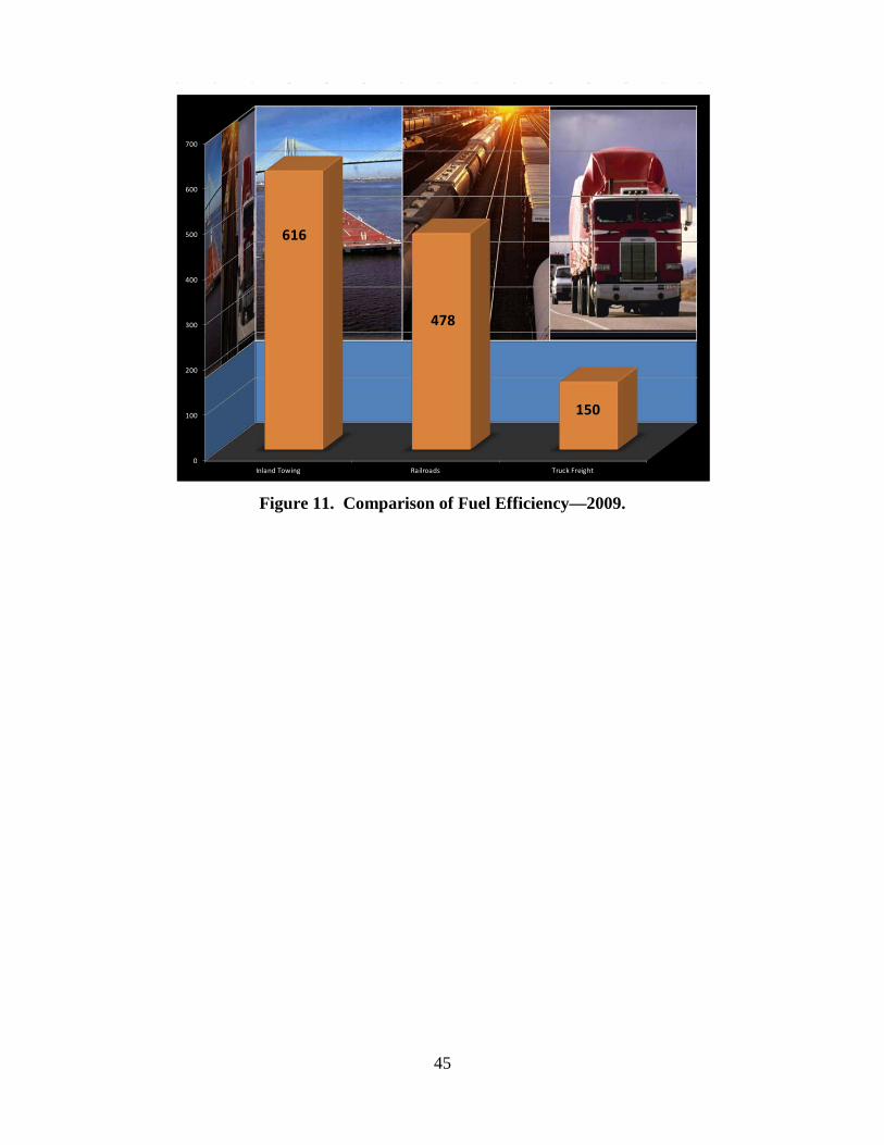
45

Figure 11. Comparison of Fuel Efficiency—2009.

0

100

200

300

400

500

600

700

Inland Towing Railroads Truck Freight

616

478

150

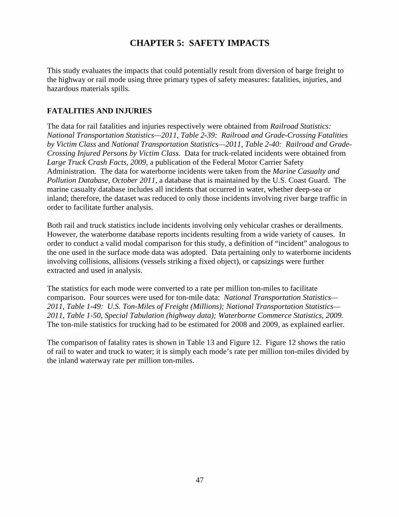
47

CHAPTER 5: SAFETY IMPACTS This study evaluates the impacts that could potentially result from diversion of barge freight to the highway or rail mode using three primary types of safety measures: fatalities, injuries, and hazardous materials spills.

FATALITIES AND INJURIES

The data for rail fatalities and injuries respectively were obtained from Railroad Statistics: National Transportation Statistics—2011, Table 2-39: Railroad and Grade-Crossing Fatalities by Victim Class and National Transportation Statistics—2011, Table 2-40: Railroad and Grade-Crossing Injured Persons by Victim Class. Data for truck-related incidents were obtained from Large Truck Crash Facts, 2009, a publication of the Federal Motor Carrier Safety Administration. The data for waterborne incidents were taken from the Marine Casualty and Pollution Database, October 2011, a database that is maintained by the U.S. Coast Guard. The marine casualty database includes all incidents that occurred in water, whether deep-sea or inland; therefore, the dataset was reduced to only those incidents involving river barge traffic in order to facilitate further analysis. Both rail and truck statistics include incidents involving only vehicular crashes or derailments. However, the waterborne database reports incidents resulting from a wide variety of causes. In order to conduct a valid modal comparison for this study, a definition of “incident” analogous to the one used in the surface mode data was adopted. Data pertaining only to waterborne incidents involving collisions, allisions (vessels striking a fixed object), or capsizings were further extracted and used in analysis. The statistics for each mode were converted to a rate per million ton-miles to facilitate comparison. Four sources were used for ton-mile data: National Transportation Statistics—2011, Table 1-49: U.S. Ton-Miles of Freight (Millions); National Transportation Statistics—2011, Table 1-50, Special Tabulation (highway data); Waterborne Commerce Statistics, 2009. The ton-mile statistics for trucking had to be estimated for 2008 and 2009, as explained earlier. The comparison of fatality rates is shown in Table 13 and Figure 12. Figure 12 shows the ratio of rail to water and truck to water; it is simply each mode’s rate per million ton-miles divided by the inland waterway rate per million ton-miles.

48

Table 13. Fatality Statistics by Mode—2001–2009.

Mode

Annual Ton-

miles* (million)

Fatalities (Operator) Fatalities (Other) Total Fatalities

Total Annual* Rate** Total

Annual* Rate** Total Annual* Rate**

Highway 1,249,032 1,188 0.000951137 (13117%) 3,594 0.002877428

(13228%) 4,782 0.003829 (13200%)

Railroad 1,640,537 21 0.000012801 (177%) 861 0.000512637

(2357%) 862 0.000525 (1812%)

Water 275,826 2 0.000007251 6 0.000021753 8 0.000029

*9-year average ** Per Million Ton-Miles

0

20

40

60

80

100

120

140

Inland Towing Railroads Truck Freight

18.1

132.0

Figure 12. Ratio of Fatalities per Million Ton-Miles Versus Inland Marine—2001–2009.

Figure 13 is similar to Figure 12. It shows the ratio of rail to water and truck to water; it is simply each mode’s rate per million ton-miles divided by the inland waterway rate per million ton-miles.

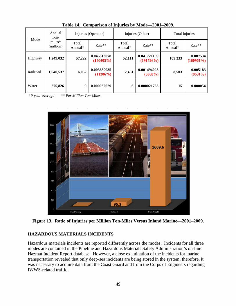
49

Table 14. Comparison of Injuries by Mode—2001–2009.

Mode

Annual Ton-

miles* (million)

Injuries (Operator) Injuries (Other) Total Injuries

Total Annual* Rate** Total

Annual* Rate** Total Annual* Rate**

Highway 1,249,032 57,222 0.045813078 (140405%) 52,111 0.041721109

(191796%) 109,333 0.087534 (160961%)

Railroad 1,640,537 6,052 0.003689035 (11306%) 2,451 0.001494023

(6868%) 8,503 0.005183 (9531%)

Water 275,826 9 0.000032629 6 0.000021753 15 0.000054

* 9-year average ** Per Million Ton-Miles

0

200

400

600

800

1000

1200

1400

1600

1800

Inland Towing Railroads Truck Freight

95.3

1609.6

Figure 13. Ratio of Injuries per Million Ton-Miles Versus Inland Marine—2001–2009.

HAZARDOUS MATERIALS INCIDENTS

Hazardous materials incidents are reported differently across the modes. Incidents for all three modes are contained in the Pipeline and Hazardous Materials Safety Administration’s on-line Hazmat Incident Report database. However, a close examination of the incidents for marine transportation revealed that only deep-sea incidents are being stored in the system; therefore, it was necessary to acquire data from the Coast Guard and from the Corps of Engineers regarding IWWS-related traffic.

50

The Coast Guard stores information on all incidents involving marine transportation while the Corps of Engineers reports tonnage and ton-mile statistics. The Corps reports the commodities according to Standard International Trade Classification (SITC) code, a statistical classification system designed by the United Nations for commodities in international trade to provide the commodity aggregates needed for purposes of economic analysis and to facilitate the international comparison of trade-by-commodity data. The data reported by the Pipeline and Hazardous Materials Safety Administration (PHMSA) use United Nations UN Identification Numbers for tracking commodities. Since the objective of this analysis is to develop an incident rate (as opposed to a comparison of how much of a given product is spilled), the PHMSA spill and ton-mile data are used for truck and rail statistics, while the Coast Guard and Corps data are used for the waterborne activity. The Coast Guard transitioned to a new marine casualty tracking system in late 2001. Prior reviews have indicated that some of the data from 2001 were not picked up in the newer system. Since this report covers 2001–2009, it was necessary to review the data for both systems for 2001, while the newer system was used exclusively for 2002–2009. The earlier system was known as the Marine Safety Information System (MSIS). The current system is referred to as the Marine Information for Safety and Law Enforcement (MISLE) system. The Coast Guard data do not segregate deep-sea incidents from IWWS incidents, so the research team extracted the spills related to IWWS traffic. Because all three reporting systems basically rely on self-reporting, and the definitions of materials that require reporting are very complex, much of the spill data are suspect. However, for larger spills, it seems reasonable to assume that the accuracy of the data improves, due to the severity of the incident and public scrutiny; therefore, the research team decided to analyze only large spills as a measure of the overall safety of the modes in the area of spills. The threshold quantity was set at 1,000 gallons. Table 15 and Figure 14 provide a comparison of spills across the modes:

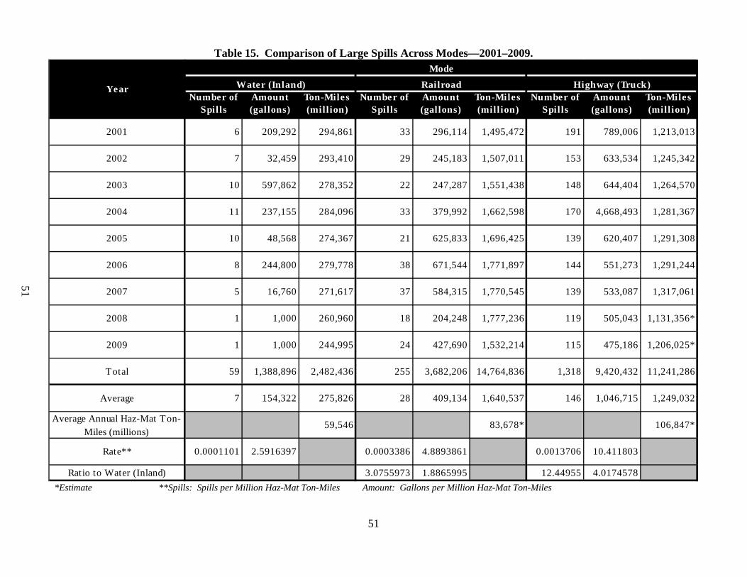
51

51

Table 15. Comparison of Large Spills Across Modes—2001–2009.

Number of Spills

Amount (gallons)

Ton-Miles (million)

Number of Spills

Amount (gallons)

Ton-Miles (million)

Number of Spills

Amount (gallons)

Ton-Miles (million)

2001 6 209,292 294,861 33 296,114 1,495,472 191 789,006 1,213,013

2002 7 32,459 293,410 29 245,183 1,507,011 153 633,534 1,245,342

2003 10 597,862 278,352 22 247,287 1,551,438 148 644,404 1,264,570

2004 11 237,155 284,096 33 379,992 1,662,598 170 4,668,493 1,281,367

2005 10 48,568 274,367 21 625,833 1,696,425 139 620,407 1,291,308

2006 8 244,800 279,778 38 671,544 1,771,897 144 551,273 1,291,244

2007 5 16,760 271,617 37 584,315 1,770,545 139 533,087 1,317,061

2008 1 1,000 260,960 18 204,248 1,777,236 119 505,043 1,131,356*

2009 1 1,000 244,995 24 427,690 1,532,214 115 475,186 1,206,025*

Total 59 1,388,896 2,482,436 255 3,682,206 14,764,836 1,318 9,420,432 11,241,286

Average 7 154,322 275,826 28 409,134 1,640,537 146 1,046,715 1,249,032

Average Annual Haz-Mat Ton-Miles (millions)

59,546 83,678* 106,847*

Rate** 0.0001101 2.5916397 0.0003386 4.8893861 0.0013706 10.411803

Ratio to Water (Inland) 3.0755973 1.8865995 12.44955 4.0174578

Water (Inland) Railroad Highway (Truck)Mode

Year

*Estimate **Spills: Spills per Million Haz-Mat Ton-Miles Amount: Gallons per Million Haz-Mat Ton-Miles

52

0

2

4

6

8

10

12

Inland Towing Railroads Truck Freight

2.594.89

10.41

Figure 14. Gallons Spilled per Million Haz-Mat Ton-Miles (2001–2009).

What the statistics do not show (and this project does not attempt to analyze) is the effect such incidents have on the human population. Because they use infrastructure shared with the general public—infrastructure which has a high utilization rate by the general public or is in close proximity to large numbers of people—spills from truck and rail incidents are more likely to pose an immediate threat to the health of human beings than marine incidents. Waterborne transportation, by virtue of the fact that it occurs on a river, is less likely to pose an immediate threat to human beings, although it may have a detrimental effect on aquatic flora and fauna. The project team attempted to compare the cost of property damages from hazardous materials incidents, but the data are extremely unreliable, so this analysis was not performed.

53

CHAPTER 6: INFRASTRUCTURE IMPACTS The question addressed in this part of the analysis is, “What are the potential impacts to rail and highway infrastructure caused by a hypothetical diversion of waterborne traffic to either mode?” In order to compare the impacts of a theoretical diversion of waterborne freight transportation to surface transportation with respect to land infrastructure, the effects of a situation where the waterways are closed and all cargo is forced to move either by rail or truck are evaluated. It is a highly unlikely event, but such an analysis helps evaluate the potential savings to the nation due to the utilization of waterborne transportation.

PAVEMENT DETERIORATION

Roadway pavements need to be designed at a level of structural capacity that can withstand the repeated loadings inflicted by heavy trucks. Passenger cars inflict minimal damage to the pavement by comparison. The Structural Number (SN) measures pavement structural capacity and new pavements–which are at “full strength”– have a SN of 4.5–5.0. The useful life of a new pavement is approximately 20 years, at which point the SN drops to about 2.5 and major rehabilitation is required. The total load expected over the pavement’s “lifetime” due to heavy truck traffic is the primary input in calculating the thickness of a new pavement. Previous chapters have defined the “standard” truck to be used in the event of a waterborne freight diversion as the combination tractor-semitrailer truck with GVWR of 80,000 lbs. Figure 15 shows the axle configuration of this type of truck. There are five axles total, one steering axle, and four remaining axles in pairs, called “tandem axles”.

Figure 15. Semitrailer configuration 3-S2: the 18-wheeler. A tandem axle involves two single axles close together and inflicts less pavement damage than two single axles further apart. The integrated load a truck exerts on a pavement is estimated by the number of Equivalent 18,000-pound (or 18-kip) Single Axle Loads or ESAL using the

12,000 lbs Steering

Axle

36,000 lbs Tandem

Axle

32,000 lbs Tandem

Axle

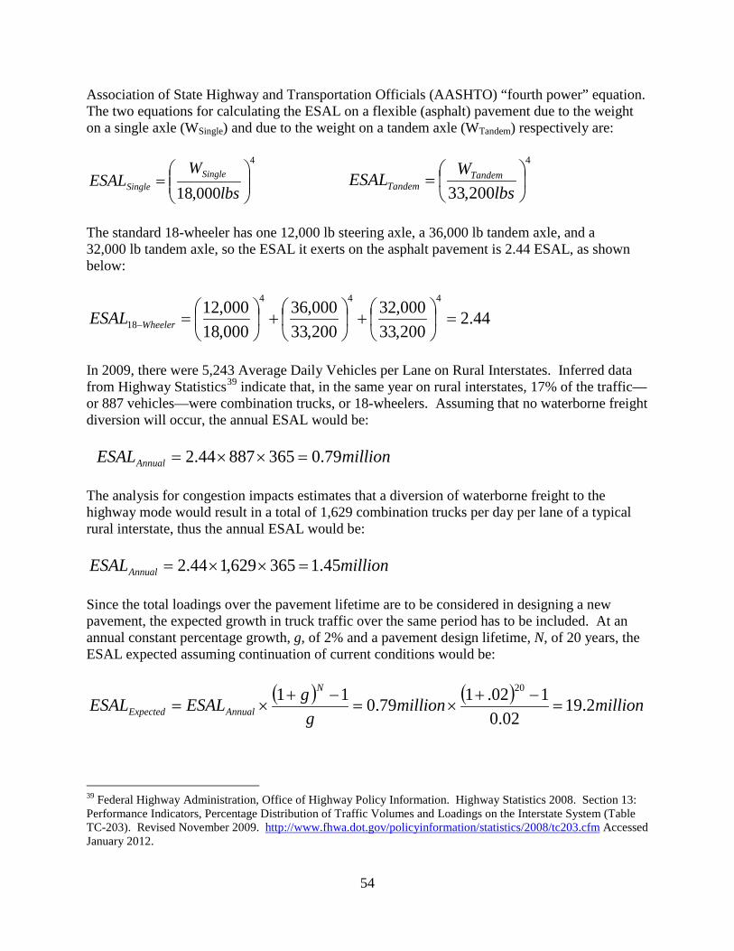
54

Association of State Highway and Transportation Officials (AASHTO) “fourth power” equation. The two equations for calculating the ESAL on a flexible (asphalt) pavement due to the weight on a single axle (WSingle) and due to the weight on a tandem axle (WTandem) respectively are:

4

000,18

=

lbsW

ESAL SingleSingle

4

200,33

=lbs

WESAL TandemTandem

The standard 18-wheeler has one 12,000 lb steering axle, a 36,000 lb tandem axle, and a 32,000 lb tandem axle, so the ESAL it exerts on the asphalt pavement is 2.44 ESAL, as shown below:

44.2200,33000,32

200,33000,36

000,18000,12

444

18 =

+

+

=−WheelerESAL

In 2009, there were 5,243 Average Daily Vehicles per Lane on Rural Interstates. Inferred data from Highway Statistics39 indicate that, in the same year on rural interstates, 17% of the traffic—or 887 vehicles—were combination trucks, or 18-wheelers. Assuming that no waterborne freight diversion will occur, the annual ESAL would be: millionESALAnnual 79.036588744.2 =××= The analysis for congestion impacts estimates that a diversion of waterborne freight to the highway mode would result in a total of 1,629 combination trucks per day per lane of a typical rural interstate, thus the annual ESAL would be:

millionESALAnnual 45.1365629,144.2 =××= Since the total loadings over the pavement lifetime are to be considered in designing a new pavement, the expected growth in truck traffic over the same period has to be included. At an annual constant percentage growth, g, of 2% and a pavement design lifetime, N, of 20 years, the ESAL expected assuming continuation of current conditions would be:

( ) ( ) millionmilliong

gESALESALN

AnnualExpected 2.1902.0

102.179.011 20

=−+

×=−+

×=

39 Federal Highway Administration, Office of Highway Policy Information. Highway Statistics 2008. Section 13: Performance Indicators, Percentage Distribution of Traffic Volumes and Loadings on the Interstate System (Table TC-203). Revised November 2009. http://www.fhwa.dot.gov/policyinformation/statistics/2008/tc203.cfm Accessed January 2012.

55

Similarly, assuming a waterborne freight diversion occurs, the ESAL expected over a 20-year pavement life would be:

( ) ( ) millionmilliong

gESALESALN

AnnualExpected 3.3502.0

102.145.111 20

=−+

×=−+

×=

A quick comparison of the two calculated values indicates that if a waterborne freight diversion occurs, the ESAL expected over the pavement throughout its 20-year lifetime is more than one-and-a-half times and almost double (184%) the ESAL expected under current conditions. The AASHTO guidelines for pavement design40 were then followed to determine the pavement thickness required to accommodate the ESAL expected over the pavement’s lifetime, first, assuming continuation of current conditions, and second, that a waterborne freight diversion will occur. Identical values for these remaining required parameters were used to ensure comparison on an equal basis:

• Reliability, R: 90% • Standard Deviation So: 0.35 • Serviceability Loss, ∆ PSI: 2.0 • Subgrade Strength, MR: 10,000 psi (10ksi) • Asphalt Concrete Elastic Modulus, EAC: 380,000 psi • Asphalt Concrete Surface Course Structural Layer Coefficient, a: 0.41

At the current level of ESAL expected over the pavement throughout the 20 years, the design Structural Number, SN, was found to be 4.7, which is within the range of an SN of 4.5 to 5.0 for a new pavement or a pavement at full strength—one that has undergone major rehabilitation, typically 20 years after construction. In order for clearer comparison to take place, an all-asphalt pavement is assumed, whose required thickness, d, in inches, is:

aSNd = Here, sinche

aSNd 5.11

41.07.4===

At the level of ESAL assuming freight diversion, the design Structural Number, SN, was found to be 5.0, which is natural since a higher ESAL is expected over the pavement’s lifetime. Similarly, in order for clearer comparison to take place, an all-asphalt pavement is assumed, whose required thickness, d, in inches, is:

aSNd = Here, inches

aSNd 2.12

41.00.5===

Comparison of the thickness results implies that in the event of a waterborne freight diversion, a flexible pavement on an average rural interstate would require an additional 0.7 inches of asphalt layer in order to adequately withstand the 20-year loadings of combination trucks without requiring premature major rehabilitation (before the 20 years expire). The asphalt thickness 40 American Association of State Highway Transportation Officials. Guide for Design of Pavement Structures 1993 and 1998 Supplement.

56

addition would occur at the construction stage of a new pavement or as an overlay to an existing pavement so that the pavement strength rises to the required SN of 5.0 and its longevity for the next 20 years is ensured, at which point major rehabilitation will have to be undertaken. Of course, if the existing pavement is already worn, the asphalt layer thickness will have to be first brought up to the 11.5 inches, and then up to the 12.2 inches so that it is strong enough to last for the next 20 years. In the field, the additional 0.7 inches of asphalt layer calculated above would be rounded to 2 inches (assuming that this is the only reason for need of repaving and that the pavement is not already in need of repaving) which is also the minimum asphalt overlay thickness typically performed by departments of transportation. Assuming an even truck traffic distribution, a minimum 2 inches thickness of asphalt layer would have to be added to the pavement of 122,039 lane-miles of rural interstate41 given the higher levels of expected 20-year truck loadings.

Further Highway Infrastructure Impacts

The system-wide impacts to infrastructure can be put into perspective when it is borne in mind that the rural segments of the interstate system consist of 122,039 lane-miles. In addition, there are over 8 million lane-miles classified under other functional highway systems nationally. Corridors that are parallel to the major rivers considered would undoubtedly receive a higher concentration of the additional truck traffic, and would be affected to a higher degree than the national average. This analysis assumed that truck traffic would be equally distributed over all lanes, but in reality this may not be always true. In rural road segments with a low density of entry and exit ramps the outer lane is used by trucks more heavily and the pavement in that lane sustains considerably higher levels of damage than the inner lane. It is beyond the scope of this analysis to accurately predict, analyze, or associate any monetary cost with other possible infrastructure impacts or improvements that would be required in the event of a waterborne freight diversion to heavy trucks. However, a transportation engineer can safely rely on past trends and experience to argue that these would include improvements in the form of capital expenditures on new construction of infrastructure and facilities such as bridges, ramps, highway geometric features such as horizontal and vertical curves and shoulders, truck

41 Federal Highway Administration, Office of Highway Policy Information. Highway Statistics 2009. Section 4: Highway Infrastructure, Public Road Lane-Miles by Functional System 1980–2009 (Table HM-260). January 2011. http://www.fhwa.dot.gov/policyinformation/statistics/2009/hm260.cfm Accessed January 2012.

Higher levels of heavy truck traffic typically require significant capital expenditure on bridges, ramps, highway geometric features such as horizontal and vertical curves and shoulders, truck stops, weigh stations, traffic control, etc., as well as higher routine maintenance costs.

Assuming an even truck traffic distribution, a minimum 2 inch thickness of asphalt layer would have to be added to the pavement of 122,039 lane-miles of rural interstate given the higher levels of expected 20-year truck loadings.

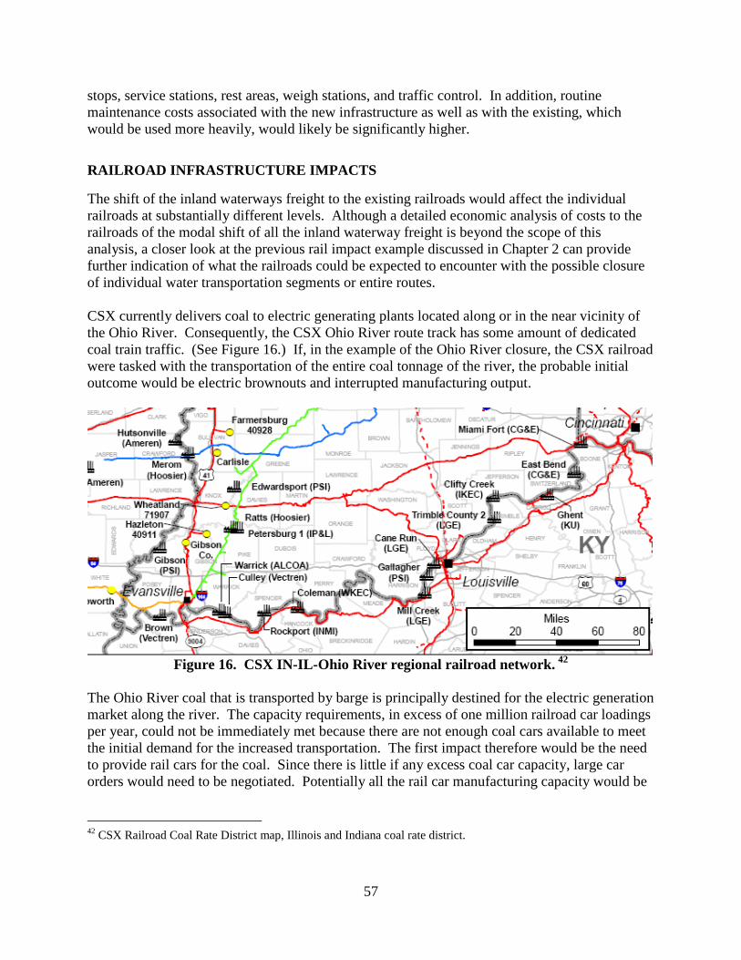
57

stops, service stations, rest areas, weigh stations, and traffic control. In addition, routine maintenance costs associated with the new infrastructure as well as with the existing, which would be used more heavily, would likely be significantly higher.

RAILROAD INFRASTRUCTURE IMPACTS

The shift of the inland waterways freight to the existing railroads would affect the individual railroads at substantially different levels. Although a detailed economic analysis of costs to the railroads of the modal shift of all the inland waterway freight is beyond the scope of this analysis, a closer look at the previous rail impact example discussed in Chapter 2 can provide further indication of what the railroads could be expected to encounter with the possible closure of individual water transportation segments or entire routes. CSX currently delivers coal to electric generating plants located along or in the near vicinity of the Ohio River. Consequently, the CSX Ohio River route track has some amount of dedicated coal train traffic. (See Figure 16.) If, in the example of the Ohio River closure, the CSX railroad were tasked with the transportation of the entire coal tonnage of the river, the probable initial outcome would be electric brownouts and interrupted manufacturing output.

Figure 16. CSX IN-IL-Ohio River regional railroad network. 42

The Ohio River coal that is transported by barge is principally destined for the electric generation market along the river. The capacity requirements, in excess of one million railroad car loadings per year, could not be immediately met because there are not enough coal cars available to meet the initial demand for the increased transportation. The first impact therefore would be the need to provide rail cars for the coal. Since there is little if any excess coal car capacity, large car orders would need to be negotiated. Potentially all the rail car manufacturing capacity would be

42 CSX Railroad Coal Rate District map, Illinois and Indiana coal rate district.

58

required to meet the initial car demand requirement. An estimation of a typical unit coal car cost is approximately $80,000 each.43 Additional dedicated locomotives would also be required to be added to operate the new coal trains as coal cars are delivered to the system. Typical locomotive costs are estimated to be $2,000,000 each. The number of rail cars needed can be estimated by making a few assumptions. First, the cycle time for the typical river diverted traffic to a coal train might only be two days from the coalmine to the utility and returning to the mine. However, since all train traffic may be assumed to be much slower because of the large amount of new traffic, existing coal trains sharing the affected routes would also have their cycle times increased, or, in other words, all coal trains using the route would be slowed down to the three day cycle time used elsewhere in this report. A requirement of 1,054,160 coal loadings using 108 car unit trains will require 9,760 unit train movements per year. Assuming that each train requires three days per trip and there are only 365 days in the year, each train can only make 121.7 trips per year. Dividing the number of train initiations by the number of train trips per year for 80.22 train sets. It is assumed any partial train set must be added as a whole train set, so there will need to be 81 train sets. Typical coal trains of 100 or more loaded coal cars require three locomotives to operate safely and efficiently. A conservative estimate of 243 new locomotives would be needed to provide power for the new trains. The total number of new cars needed to meet the requirements for 81 new train sets is 8,748. The price tag for 243 new locomotives at a unit cost of $2,000,000 each is $486,000,000. At a unit cost of $80,000 each, the 8,748 new coal cars will cost $699,840,000. Together, the minimum equipment cost would be $1,185,840,000. Many regulatory issues, operating concerns, and constraints are excluded from this example; for instance, the fact that every locomotive is required by regulation to have a substantial inspection four times each year is not considered in this example. The typical downtime for a scheduled 92-day locomotive inspection would be one day, where one day is the equivalent of one work shift. The inspection could easily take less time; however, if there were any unexpected events requiring extra shop time for minor repairs, the inspection event could exceed a 24-hour time period. Referring to the example in Chapter 2, the system average train speed for the CSX system could go from approximately 20 mph down to less than 15 mph and as little as 7 mph, or a decrease in system velocity between 25% and 65%. While it would be unreasonable to assume that all coal traffic on the CSX system would be impacted with a decrease in cycle times equal to 43 Roanoke Times, February 21, 2011.

The diversion of Ohio River Coal would require 243 new locomotives and 8,748 new coal cars immediately.

Diversion of river traffic could be expected to cause: • Increased demand for rail cars and

locomotives • Higher freight rates • Need to expand infrastructure (rail lines) • Slower and less reliable delivery times

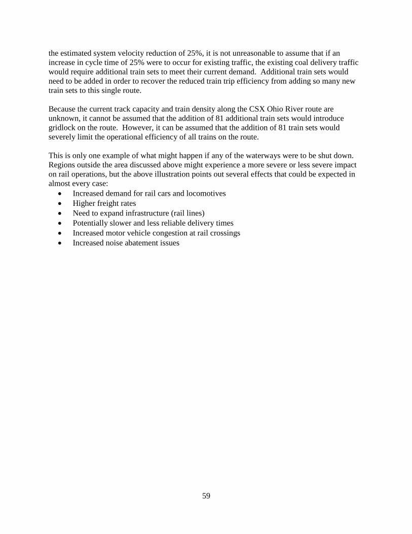
59

the estimated system velocity reduction of 25%, it is not unreasonable to assume that if an increase in cycle time of 25% were to occur for existing traffic, the existing coal delivery traffic would require additional train sets to meet their current demand. Additional train sets would need to be added in order to recover the reduced train trip efficiency from adding so many new train sets to this single route. Because the current track capacity and train density along the CSX Ohio River route are unknown, it cannot be assumed that the addition of 81 additional train sets would introduce gridlock on the route. However, it can be assumed that the addition of 81 train sets would severely limit the operational efficiency of all trains on the route. This is only one example of what might happen if any of the waterways were to be shut down. Regions outside the area discussed above might experience a more severe or less severe impact on rail operations, but the above illustration points out several effects that could be expected in almost every case:

• Increased demand for rail cars and locomotives • Higher freight rates • Need to expand infrastructure (rail lines) • Potentially slower and less reliable delivery times • Increased motor vehicle congestion at rail crossings • Increased noise abatement issues

APPENDIX A: COMPARATIVE CHARTS

A-1

Table 16. Summary of Emissions—Grams per Ton-Mile—2005 & 2009. Emissions (grams/ton-mile)

Mode HC/VOC CO NOx PM CO2

2005 2009 2005 2009 2005 2009 2005 2009 2005 2009

Inland Towing 0.01737 0.01680 0.04621 0.04470 0.46907 0.45390 0.01164 0.01130 17.48 16.920

Railroad 0.02421 0.021925 0.06440 0.058321 0.65368 0.591975 0.01623 0.01469 24.39 22.0800

Truck 0.12 0.10 0.46 0.37 1.90 1.45 0.08 0.06 171.87 171.83

A-2

0

10000

20000

30000

40000

50000

60000

70000

Inland Towing Railroads Truck Freight

60,96657,208

41,01947,308

7,599 5,820

2005 | 2009

2005 | 2009

2005 | 2009

Figure 17. Ton-Miles per Ton of GHG (2005 & 2009).

A-3

0

20

40

60

80

100

120

140

160

180

Inland Towing Railroads Truck Freight

16.417.48 24.38 21.13

171.87 171.83

2005 | 20092005 | 2009

2005 | 2009

Figure 18. Tons of GHG per Million Ton-Miles (2005 & 2009).

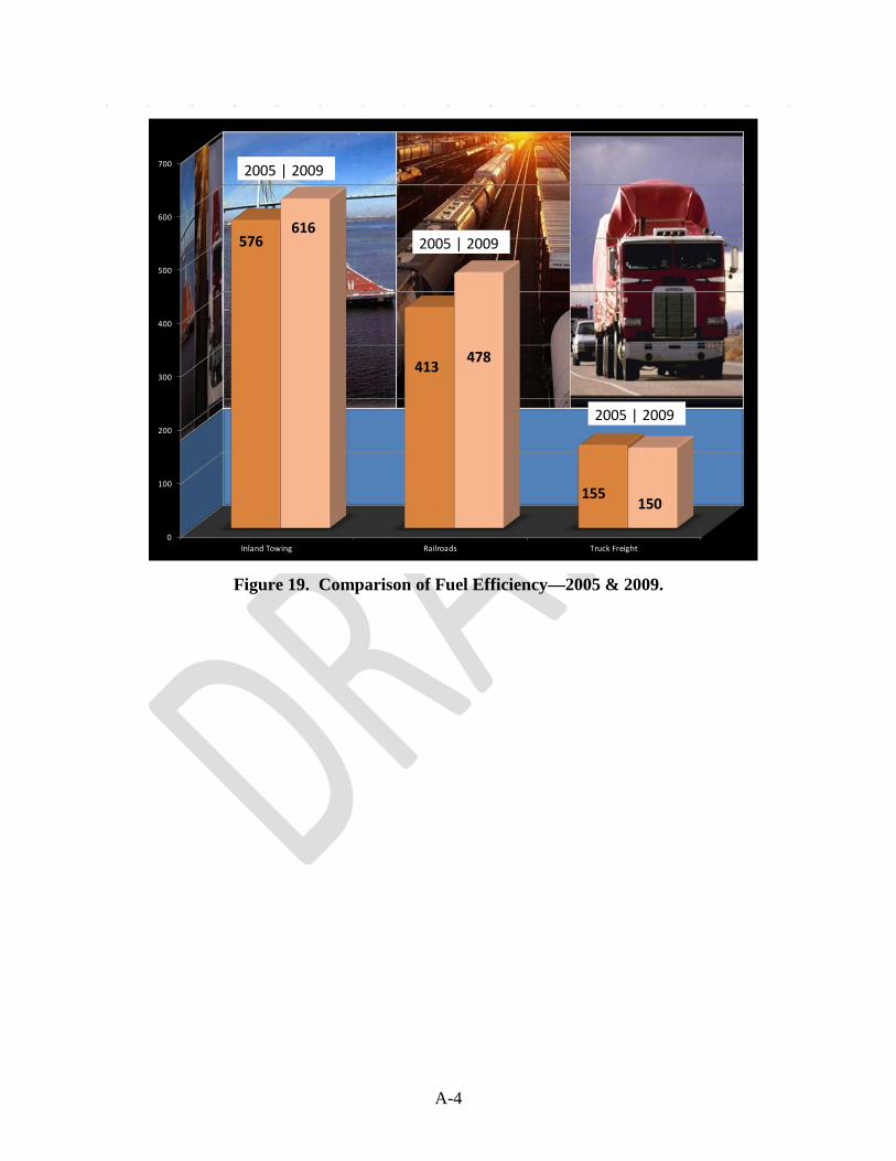
A-4

0

100

200

300

400

500

600

700

Inland Towing Railroads Truck Freight

2005 | 2009

2005 | 2009

2005 | 2009

576616

413 478

155150

Figure 19. Comparison of Fuel Efficiency—2005 & 2009.

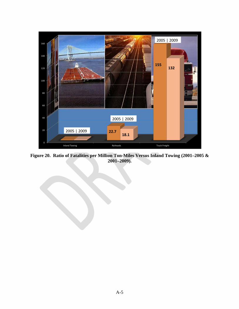
A-5

0

20

40

60

80

100

120

140

160

Inland Towing Railroads Truck Freight

22.718.1

155132

2005 | 2009

2005 | 2009

2005 | 2009

Figure 20. Ratio of Fatalities per Million Ton-Miles Versus Inland Towing (2001–2005 &

2001–2009).

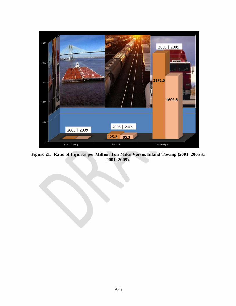
A-6

0

500

1000

1500

2000

2500

Inland Towing Railroads Truck Freight

95.3125.2

2171.5

1609.6

2005 | 20092005 | 2009

2005 | 2009

Figure 21. Ratio of Injuries per Million Ton-Miles Versus Inland Towing (2001–2005 &

2001–2009).

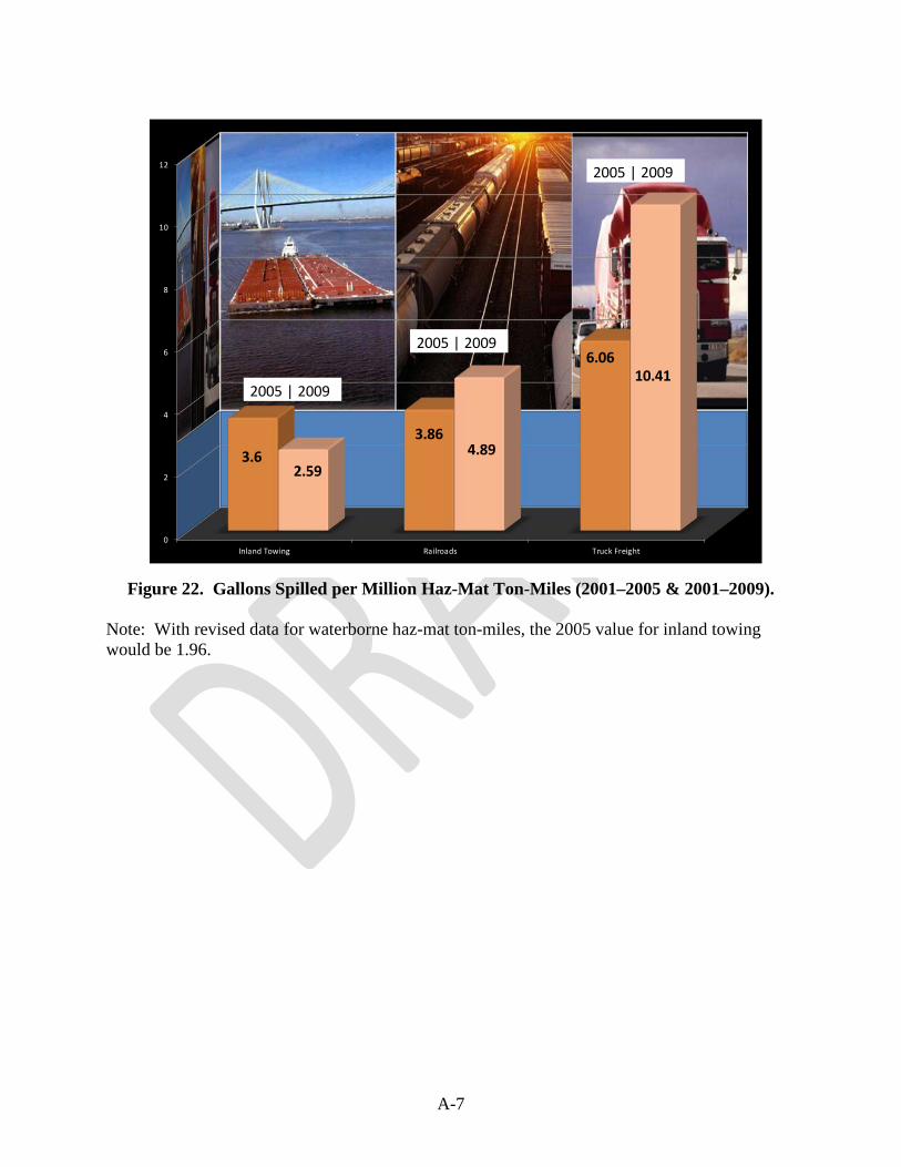
A-7

0

2

4

6

8

10

12

Inland Towing Railroads Truck Freight

3.63.86

6.06

4.89

10.41

2.59

2005 | 2009

2005 | 2009

2005 | 2009

Figure 22. Gallons Spilled per Million Haz-Mat Ton-Miles (2001–2005 & 2001–2009).

Note: With revised data for waterborne haz-mat ton-miles, the 2005 value for inland towing would be 1.96.