A Microcomputer-Based Conducting Systempagiamt/kcsmith/...baecker-conducting-system.pdf · based...

W. Buxton, W. Reeves, G. Fedorkow, K. C. Smith, and R. Baecker. Structured Sound Synthesis Project Computer Systems Research Group University of Toronto Toronto, Ontario Canada M5S 1A4

A Microcomputer- based Conducting System

Introduction The subject of this paper is a portable, microcomputer-based performance system that we call the conduct system.1 This system was developed at the University of Toronto as part of the research of the Structured Sound Synthesis Project (SSSP) (Buxton, Fogels, Fedorkow and Smith 1978). The system, built around a microprocessor controlling a digital sound synthesizer, had its genesis in the earlier conductor system of Mathews (Mathews 1976). That is, it is a system that allows the performer to interpret or conduct precomposed score material, rather than a system on which the prime performance task is to articulate each individual note, as is the case with conventional instruments.

In the remainder of this paper, we shall provide a description of the microcomputer-based conducting system, concentrating on aspects of the human interface and the control structure. In addition, we shall discuss what we see as the relative strengths and weaknesses of the system, based on our experi- ence with it in both the laboratory and the concert hall. We shall begin, however, by relating our work to that of others in the field, and by discussing the general issues of the problem.

Background The past three decades have seen an ever increasing interest in electroacoustic music (Battier and Arveil- ler 1978; Buxton 1977; Cross 1976). To date, how-

ever, most compositions (Davies 1968; Melby 1976) have been studio productions that are performed by tape playback in a concert hall. This situation is largely due to the available hardware's limited ability to provide adequate real-time control over musical complexity. The advent of the voltage-controlled synthesizer (Moog 1965) saw the beginnings of a change in this situation, but it has only been since the recent introduction of digital technology that the full potential of the performance situation shows hope of being realized. This was first seen in portable hybrid systems such as those of Buchla (1978), Ko- brin (1975), and Bartlett (1979). More recently, all- digital performance systems have been introduced and successfully used in concert (New England Digi- tal 1978).

The implied notion of performance imbedded in these systems is an important consideration in their comparison.2 In this regard, one basis for distinction is the amount of real-time musical decision making supported: performance by tape recorder and impro- visation on a conventional instrument represent two extremes. Given this basis, a second criterion for distinction is the structural level that can be affected by this decision making. That is, where does the enabled decision making fall in between the global decisions affecting high-level structures and the low-level decisions affecting individual notes?3 The role of the conductor in a symphony orchestra is an example of the former; the role of an instrumentalist within that orchestra is an example of the latter. Finally, in discussing electronic systems that may be programmed to have a certain amount of musical "intelligence," we can introduce one more criterion

1. This paper has grown out of an earlier one (Buxton, Reeves, Fedorkow, Smith, and Baecker 1979) which was presented at the 64th Convention of the Audio Engineering Society. While certain parts of the text are the same, the bulk of the paper has been rewritten and expanded to better represent the current state of the system and the interests of the readers of Computer Music Journal.

2. The discussion that follows owes much to conversations with Max V. Mathews of Bell Telephone Labs, Murray Hill, New Jersey, during his visit to Toronto in the spring of 1978. 3. To use terminology derived from linguistics (Chomsky 1972), at what levels is decision making facilitated in terms of the "deep" and "surface" structure?

8 A Microcomputer-based Conducting System

Fig. 1. Three-dimensional space used to characterize performance systems.

Distribution of decision making

Level of decision making

Amount of decision making

Fig. 2. System architecture.

SSSP I/O LSI- 11/2 Digital Transducers Microcomputer Synthesizer

File 4 Channels

System .

Audio Output (floppy disks)

for distinction: physically, where does the decision making take place? That is, how is the real-time decision making distributed between the musician and the machine? Bartlett's system is a good example of musical decision making being divided between the two.

Together, these three criteria define a three- dimensional space (Fig. 1) that can be used to characterize performance systems. In terms of this space, like most of the systems mentioned ours enables the performer to exercise a fairly high degree of real-time decision making. In contrast, however, the current implementation is optimized so as to express control over syntactic structures above the note level. The composer performs or interprets precomposed material (in a manner analogous to the role of the orchestral conductor) rather than articulating the music note by note (in a manner analogous to that of an instrumentalist). Finally, in the implementation to be described, all decision making in this process remains with the human performer/conductor.

Architecture A functional block diagram of the system's architecture is presented in Fig. 2. As is shown in Fig. 2, the main functional units of the system are the control transducers, the microcomputer, a file system, and the sound synthesizer.

The Synthesizer

The synthesizer used in the conduct system (Bux- ton, Fogels, Fedorkow, and Smith 1978), was developed at the University of Toronto as part of the research of the SSSP. It is an all-digital device capable of generating complex, high-fidelity audio sig- nals according to well-known synthesis techniques including additive synthesis (Moorer 1977), VOSIM (Kaegi and Tempelaars 1978), frequency modulation (Chowning 1973), and waveshaping (Le Brun 1978; Arfib 1978). Through the use of time-division mul- tiplexing, it functionally achieves 16 oscillators, each of which has a sampling rate of 50 KHz. The output of these oscillators can be routed to one of four audio output channels.

The Computer

In selecting a computer upon which to base the system, we were guided by the constraints of cost- effectiveness, portability, and a reasonably high computational bandwidth. While existing 8-bit mi- croprocessors were compact and affordable from a hardware point of view, they had neither the required computational power nor the software tools we felt were required. This latter point was of particular importance in terms of cost-effectiveness from the software point of view. We already had a large investment in software running on our PDP- 11/45 (DEC 1973), so the optimal choice would be downward compatible with our existing system. We chose the DEC LSI-11/2 (DEC 1976). Not only did this allow us to run existing programs on the smaller processor, but it also enabled us to continue writing all new software in a high level language ("C") (Ker-

Buxton, Reeves, Fedorkow, Smith, and Baecker 9

Fig. 3. The synthesizer with disk drive and microcomputer (CPU) (photo credit: Robert Hudyma).

.'W"

.

. . . . ...

.. .. . ..

...... ... Pit ? i

-.

16. •i

00460.:

IV vs F N' .*

Hi W. Pan Z .'O'n'

!i• • }}• ..... . .. •::. •.• '!Q •:••;i;....

....... ..'•:::... •..

.... ;: la Ma

ai 4 ,; pkn_ X8CI: 46i:::r~

%a gg I ......... ell ON

Fig. 4. Integration of composition and performance systems.

Composition PDP-11/45 Control Computer TransducersHigh-Speed

Parallel Direct Memory Access Interface

Performance LSI-11/2 SSSP Digital Control Microcomputer Sound Transducers Synthesizer

nighan and Ritchie 1978) on the more powerful PDP-11/45. The importance of this, in terms of the efficiency of software development, was all the more pronounced in that it allowed us to continue using the software tools available under the UNIX operat- ing system (Ritchie and Thompson 1974). The microcomputer is physically housed in the same cabinet as the digital synthesizer. A sense of the size of the system can be gained from Fig. 3, which is a photograph showing the synthesizer, microcomputer, and floppy-disk system.

The File System

One of the consequences of having a portable system is that some nonvolatile storage medium is required in order to be able to bootstrap the system as well as to retrieve programs and musical data. One alterna-

tive is to simply save a core image on a serial storage device (such as a cassette or cartridge tape machine). While this provides a workable, inexpensive alternative (Buchla and associates 1978), it has two prime disadvantages; it is slow and it makes random- access file-oriented input/output very inefficient. Since the design of our data-structures (Buxton, Reeves, Baecker, and Mezei 1978) is highly file- oriented, we felt that this solution was not accept- able. For the concert situation, therefore, we chose to adopt the more expensive (but efficient) use of floppy disks.4

One important benefit accrues as a result of com- bining file-oriented approach and matching the PDP-11/45 and LSI-11/2 processors. This is seen in the laboratory environment, in which the small, portable performance system can be integrated with the larger, more powerful composition system (Fig. 4). The basis of this integration is a specially de- signed high-speed parallel direct memory access (DMA) link between the two machines. From the point of view of the composition system, we can make use of all the resources available on the powerful but time-shared PDP-11/45, while guaranteeing the integrity of the music's timing by using the LSI-11 as a dedicated slave-processor servicing the synthesizer. In this case, the control transducers of the performance system are left unused. From the viewpoint of the performance system, we can

4. The DSD-440 dual-drive system made by Data Systems Design is used for disk storage.


Fig. 5. The studio working environment (photo credit: Robert Hudyma).

i'? ::r::

.*?. :r 31 ?;:?:

QE;

::+: ~r::?7

?~?? ???

Fig. 6. The control transducers.

CRT screen tracker

cursor switches

keyboard / tablet sliders

down-line load the conduct system from the PDP- 11/45 and run the LSI-11 as a stand-alone processor. Most importantly, however, the LSI-11 can then (via the DMA interface) use the file system of the PDP- 11/45 as if it were its own. The user can thereby avoid making redundant copies of files on floppy disks, until it is certain they are wanted in concert. The composer can compose using the most powerful resources available, then immediately "interpret" that composition using a system optimized for that purpose. Furthermore, the systems programmer can write, compile, and debug software on the more powerful PDP-11/45, then easily down-line load it into the LSI-11/2 for testing. At any time copies of files may be made on floppy disks so that the system can function at remote locations where the "umbili- cal cord" to the PDP-11/45 must be broken. The physical proximity of the work stations of the two systems can be seen in Fig. 5, a photograph showing the LSI-11 (conduct) station in the foreground, and the 11/45's graphics display in the background.

Control Transducers

The control transducers used by the system are diagrammed in Fig. 6. These transducers consist of three main devices: a terminal, a tablet, and slider box.5

The terminal employed is a conventional alphanumeric cathode-ray terminal (CRT). It has a typewriter keyboard on which messages can be typed, and a video display on which data can be presented. Unlike most users of such terminals, we do not interact with the system by typing commands and having them scroll by; rather, data and controls are spatially distributed on the screen in much the same manner that knobs and dials are distributed on a mixing console. Because each datum has its own specific location and all data are constantly displayed, it is easy for the operator to verify the current status of the system, and as shall be seen, effect transformations on the data.

It is the coupling of the CRT with the graphics tablet that enables us to exploit the full potential of this use of the display. While the terminal does not include graphics capabilities, it does have one important property: it has an addressable cursor. Thus the CRT cursor (which we shall henceforth refer to as the tracker) can be made to follow, or track the relative position of the-tablet cursor. This is seen in Fig. 6, for example, where the cursor is posi- tioned on the upper right-hand corner of the tablet and the tracker on the upper right-hand corner of the display. Mounted on the cursor, which is shown in detail in Fig. 7, are four buttons. In the remainder of

5. The graphics tablet used is a BIT-PADI, manufactured by Summagraphics, Fairfield, Connecticut. The terminal, made by Volker-Craig of Waterloo, Ontario, is a standard alphanumeric CRT with addressable cursor. The slider box contains two continuous-motion treadmill-like devices manufactured by Alli- son Research, Inc., of Nashville, Tennessee, with electronics of our own design. All three devices communicate with the host through standard RS-232 serial interfaces.


Fig. 7. The four-button cursor.

Z

\ \

\1 2 3

Fig. 8. Conductible parameters.

SCORE 8VE TEMPO ARTIC AMP RICH CYCLE ON/OFF

this paper, they shall be referred to as the Z-button, and buttons 1-3. When the tracker is placed in a particular position different events can be generated depending on which button is depressed. This is a useful interaction that cannot be realized using, for example, a stylus or lightpen, without using a second hand.

In summary, the benefit of our particular choice of transducers is that we can effectively employ techniques derived from interactive computer graphics on a relatively inexpensive system. We feel that the resulting notion of downward (as opposed to upward) compatibility is one of the most important concepts demonstrated by the system.

The Nature of a Conductible Score

We have stated that the main motivation for de- veloping the system was to provide the musician with a tool that would enable precomposed scores to be conducted in performance. The next step in de- scribing the system is to clarify what is meant when we talk about scores. A score is named group of notes that has been previously composed using a composing tool such as scriva (Buxton, Sniderman., Reeves, Patel and Baecker 1979). The score may consist of a single note or a more complex structure made up of up to a maximum of about 800 notes.

Scores can be compared with sequences as used in conventional analog systems. There are two important distinctions, however. First, each note of a score may be orchestrated with a different timbre. Second, the structure need not be a monolinear string. That is, notes may overlap and the number of simultane- ous voices may vary between zero (tacet), and the maximum supported by the synthesizer (currently 16). Finally, it is important to consider the notion that a composition is made up of a number of parts (for which the division of much vocal music into soprano, alto, tenor, and bass serves as an example). For our purposes, we consider each of these parts as a separate score. Therefore in order to conduct the entire composition we must be able to conduct more than one score at a time. This we can do; the obvious benefit is that we can now express "conductorlike" gestures such as "a little more from the brass, and more staccato in the violins." By providing a facility to independently conduct several scores simultaneously, we have obtained a much-needed handle on the scope of conducting commands.

Conductible Parameters For the time being, consider the simpler task of conducting a single score. There are 7 parameters of the score that we can affect. Fig. 8 shows these parameters the way they are labeled on the system's CRT. We can now describe each of these parameters in detail.

Octave (8VE)

In composing a score, each note is notated at a specific pitch. By varying this parameter from its default value (0), one can cause the score to be performed n octaves higher or lower than originally notated.


Fig. 9. Simplified display of an active score's attributes.

SCORE 8VE TEMPO ARTIC AMP RICH CYCLE ON/OFF d emo 0 60 60 0 0 1 0

Tempo (TEMPO)

This parameter allows the speed of performance of a score to be altered. What is actually being scaled is the time interval separating the start of one note and the start of the next. As with conventional music, the tempo is specified as a metronome marking, indicating the number of beats per minute.

Articulation (ARTIC)

The previous example demonstrated how the timing between note attacks could be scaled. Articulation allows the user to scale the durations of those notes. Scaling all the durations by 0.5, for example, results in a staccatolike effect, while extending the durations beyond how they were notated causes a legatolike effect. Notice the potential here for com- pensating for room acoustics (which may be very resonant or dry, for example). Notice also that tempo is unaffected by this change. Timing between event attacks is orthogonal to the timing of event durations.

Amplitude (AMP)

The parameter of amplitude is rather straightfor- ward. It enables the performer to scale the dynamics, or loudness, of a score from how it was originally notated.

Richness (RICH)

This parameter enables us to transform the timbres of the notes from the way they were originally de- fined. The effect is similar to that of having an adjustable filter affecting the signal generated by a score. In the case of the conduct system, the effect of adjusting the parameter is intimately linked with the technique of sound synthesis employed. For cur-

rent purposes, the synthesis technique used is frequency modulation (FM) (Chowning 1973). The effect of the richness parameter, therefore, is to scale the specified "index of modulation" affecting the number of spectral components and hence the timbre of individual notes.

Cycle (CYCLE)

The function of this parameter is to enable the performer to specify what occurs when a playing score comes to its end. There are two options available: the score will stop or the score will repeat. This latter case we call cycle mode. Thus the cycle parameter is a binary switch specifying whether the score is in cycle mode or not.

On/Off (ON/OFF)

The seventh parameter is another binary switch used to control whether the score is on or off. When the value is set to 1 the score begins (is triggered); when it is changed to 0 the score stops and resets.

Techniques of Control General

At all times the status of each active score is displayed on the CRT. An active score is a score that is currently conductible. While several parts or scores may be conducted throughout the course of a performance, only eight scores may be conducted, or active, at any one time. A simplified version of the format in which these data are displayed is seen in Fig. 9. As can be seen in Fig. 9, there is a field for the score's name, as well as one for each of the seven conductible parameters. The fields are labeled and the current value of a particular parameter of a score is shown in the appropriate field opposite the score's


name. In this case, for example, both the tempo and articulation parameters of the score "demo" are set to the default value: 60.

For the purpose of control, consider the conductible parameters as falling into two categories: switches and variables. Like a light switch, a switch can be either on or off. The two switchable parameters are cycle and onloff. The others, octave, tempo, articulation, amplitude, and richness, are all continuously variable. They are scaling factors, which allow parameters to be transformed from their notated values during performance.

Direct Control

Switches To change the state of a switch, the user positions the tracker above the switch and depresses the cursor Z-button. The switch immediately changes state, and the screen is updated (1 and 0 represent on and off respectively). When finished playing, a score in cycle mode will repeat; otherwise, it will stop playing and the display will be automatically updated. A score may be stopped at any point during performance, at which time it will reset to its begin- ning and wait to be restarted. (A flag that enables a score to "pick up" from where it was interrupted also exists, but has not been made available to the user in the current implementation due to problems of screen density. Using an alphanumeric terminal, we can only display 24 x 80 characters.)

Continuously Variable Parameters

Typing One technique for changing the value of a variable during performance is to position the tracker over the variable and type the new value. If the performer wishes to transpose a score up an octave from where it was originally notated, he or she need only point at the octave field and type a 1. Alternatively, typing -1 will lower the pitch by an octave. In either case, the change takes place immediately. The screen is updated and, if the score is playing, the result heard.

The typing interaction requires two hands: one for pointing and one for typing. To facilitate this one-

handed typing, certain system-specific conventions have been adopted. First, to avoid the awkwardness of depressing the return key after typing a value, any numeric value can alternatively be terminated by depressing any nonnumeric key. Second, in order to increase the speed of typing negative numbers, the minus sign can alternatively be indicated by depressing the space bar, which is equally accessible from any point on the keyboard and whose physical ap- pearance resembles a minus sign. These redefi- nitions of the keyboard are easy to remember and they significantly improve the bandwidth and reliability that can be achieved through one-handed typing. The Last-Typed Technique While we have at- tempted to make typing as efficient as possible, in many cases it is not the most appropriate means of communication. Often during performance there is simply no time to type. One alternative exploits the observation that we often assign the same value to more than one field. The system takes advantage of this redundancy by designating cursor button-3 as the last-typed button. Placing the tracker over a variable and depressing button-3 causes the last value typed to be assigned to that variable. Again, the display is updated and the effect may be heard immediately. Default Set Another often-typed value was observed to be the default or normal value for each variable field (0 for all parameters except tempo and articulation, which have a default of 60). These are the values that cause the score to be performed "as notated." To facilitate the frequent desire to restore a parameter to its default, cursor button-2 has been designated the default button. Using the technique seen in last-typed mode, any variable can be reset to its default by placing the tracker over that parameter and depressing button-2.

Dragging Perhaps the most effective technique for directly modifying the value of a variable is the technique we call dragging. This is a direct approach analogous to reaching out and turning a knob on a console. With dragging, the tracker is placed over the variable to be updated. By moving the cursor in the vertical (y) domain, while holding down the


Fig. 10. Examples of trigger usage.

SCORE 8VE TEMPO ARTIC AMP RICH CYCLE ON/OFF test1 0 60 60 0 0 1 0 - test2 0 60 60 0 0 1 0 -

a) Parameters including the control fields (-) for remote triggering.

SCORE 8VE TEMPO ARTIC AMP RICH CYCLE ON/OFF testV1 0 60 60 0 0 1 0 9 test2 0 60 60 0 0 1 0 9

b) The same two scores with trigger 9 linked to each.

SCORE 8VE TEMPO ARTIC AMP RICH CYCLE ON/OFF testi 0 60 60 0 0 1 1 9 tesI2 0 60 60 0 0 1 1 9

T9 T10

c) The same two scores playing after a unison start triggered by firing T9, shown for the first time. If the value 10 was in the control field, rather than 9, the scores would fired by firing T10.

SCORE 8VE TEMPO ARTIC AMP RICH CYCLE ON/OFF testl 0 60 60 0 0 1 1 9 test? 0 60 60 0 0 1 0 9

T9 T10

d) The flip-flop nature of triggers. Firing T9 will cause test 1 to stop, and test 2 to start.

Z-button, the value is, in effect, "dragged" up or down.6 During this process, the screen is continually updated with the current value and the results can be heard simultaneously. There is, then, an immediately accessible virtual potentiometer available for each continuously variable parameter without any special-purpose hardware. Pots can be added, moved, or scaled using this technique without any physical change to the system. The technique is direct, fluent, intuitive, inexpensive, and only requires use of one hand. Finally, it clearly is adaptable to many other control applications, not the least of which is digital sound recording and mixing.

Indirect Control

Triggers Manual Triggers One shortcoming of the control techniques described in the preceding sections is that they only allow one parameter to be changed at a time. The deficiency of this can be seen in contexts such as unison starts; starting more than one score with a single gesture. In the case of the on/off parameter, the way around this problem is to allow several scores to be started by firing a single trigger. The use of such a trigger can be considered in two phases. The first is the set-up phase: the scores to be fired by a particular trigger are grouped together. The second is the actual trigger firing.

There are ten triggers available in the system. Two of them, triggers 9 and 10 (T9 and T10) can be fired manually. Opposite the on/off parameter for each score is a control field to which a trigger number can

6. In order to prevent values at the top of the screen from being discriminated against (in terms of "dragging-room"), the mapping of the tablet coordinates to screen coordinates leaves a margin area at the top of the tablet coordinate space.


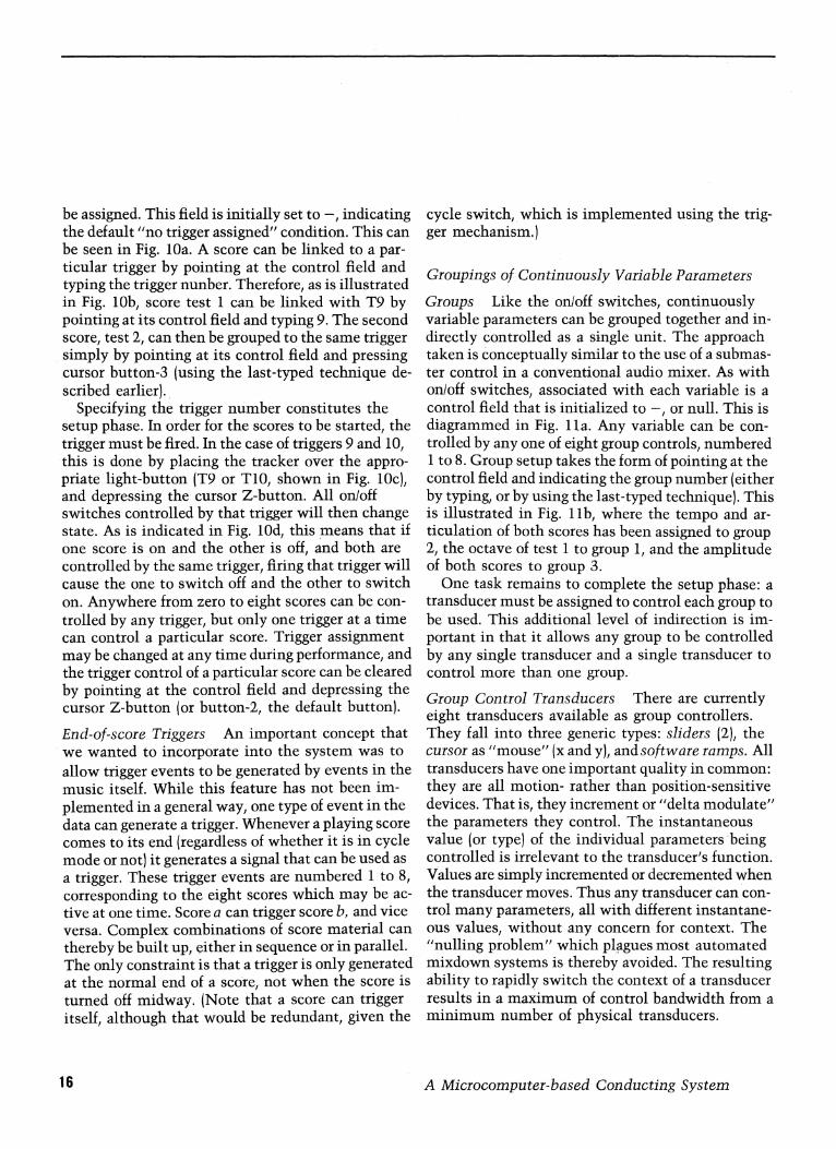
be assigned. This field is initially set to -, indicating the default "no trigger assigned" condition. This can be seen in Fig. 10a. A score can be linked to a particular trigger by pointing at the control field and typing the trigger nunber. Therefore, as is illustrated in Fig. 10b, score test 1 can be linked with T9 by pointing at its control field and typing 9. The second score, test 2, can then be grouped to the same trigger simply by pointing at its control field and pressing cursor button-3 (using the last-typed technique described earlier).

Specifying the trigger number constitutes the setup phase. In order for the scores to be started, the trigger must be fired. In the case of triggers 9 and 10, this is done by placing the tracker over the appropriate light-button (T9 or T10, shown in Fig. 10c), and depressing the cursor Z-button. All on/off switches controlled by that trigger will then change state. As is indicated in Fig. 10d, this means that if one score is on and the other is off, and both are controlled by the same trigger, firing that trigger will cause the one to switch off and the other to switch on. Anywhere from zero to eight scores can be controlled by any trigger, but only one trigger at a time can control a particular score. Trigger assignment may be changed at any time during performance, and the trigger control of a particular score can be cleared by pointing at the control field and depressing the cursor Z-button (or button-2, the default button). End-of-score Triggers An important concept that we wanted to incorporate into the system was to allow trigger events to be generated by events in the music itself. While this feature has not been implemented in a general way, one type of event in the data can generate a trigger. Whenever a playing score comes to its end (regardless of whether it is in cycle mode or not) it generates a signal that can be used as a trigger. These trigger events are numbered 1 to 8, corresponding to the eight scores which may be active at one time. Score a can trigger score b, and vice versa. Complex combinations of score material can thereby be built up, either in sequence or in parallel. The only constraint is that a trigger is only generated at the normal end of a score, not when the score is turned off midway. (Note that a score can trigger itself, although that would be redundant, given the

cycle switch, which is implemented using the trigger mechanism.)

Groupings of Continuously Variable Parameters

Groups Like the on/off switches, continuously variable parameters can be grouped together and in- directly controlled as a single unit. The approach taken is conceptually similar to the use of a submas- ter control in a conventional audio mixer. As with on/off switches, associated with each variable is a control field that is initialized to -, or null. This is diagrammed in Fig. la. Any variable can be controlled by any one of eight group controls, numbered 1 to 8. Group setup takes the form of pointing at the control field and indicating the group number (either by typing, or by using the last-typed technique). This is illustrated in Fig. 1 lb, where the tempo and articulation of both scores has been assigned to group 2, the octave of test 1 to group 1, and the amplitude of both scores to group 3.

One task remains to complete the setup phase: a transducer must be assigned to control each group to be used. This additional level of indirection is important in that it allows any group to be controlled by any single transducer and a single transducer to control more than one group. Group Control Transducers There are currently eight transducers available as group controllers. They fall into three generic types: sliders (2), the cursor as "mouse" (x and y), and software ramps. All transducers have one important quality in common: they are all motion- rather than position-sensitive devices. That is, they increment or "delta modulate" the parameters they control. The instantaneous value (or type) of the individual parameters being controlled is irrelevant to the transducer's function. Values are simply incremented or decremented when the transducer moves. Thus any transducer can control many parameters, all with different instantaneous values, without any concern for context. The "nulling problem" which plagues most automated mixdown systems is thereby avoided. The resulting ability to rapidly switch the context of a transducer results in a maximum of control bandwidth from a minimum number of physical transducers.


Fig. 11. The use of groups.

SCORE 8VE TEMPO ARTIC AMP RICH CYCLE ON/OFF testi 0 - 60 - 60 - 0 - 0 - 1 0 - test2 0 - 60 - 60 - 0 - 0 - 1 0 -

GROUPS RAMPS TRIGGERS G1 - a 0 0 T9 G2 - b 0 0 T10 03 - c 0 0 G4- d 0 0 G5 - G6 - G7 -

a) A simplified view of the screen layout showing the control fields (marked by the - character) for both score parameters and groups.

SCORE 8VE TEMPO ARTIC AMP RICH CYCLE ON/OFF testl 0 1 60 2 60 2 0 3 0 - 1 0 - test2 0 - 60 2 60 2 0 3 0 - 1 0 -

GROUPS RAMPS TRIGGERS G1 sldrl a 5 1 T9 G2 s1dr2 b 5 -2 T1i G3 x c 0 0 G4 - d 0 0 G5 - G6 - G7 - G8 -

b) The use of groups is illustrated. Group 2 is controlled by slider two. The articulation and tempo of both scores are members of this group. The octave of test 1 is the only member of group one which is controlled by slider one. The amplitudes of the two scores form group three, which is controlled by the x-mouse.

A transducer can be assigned to a group by pointing at the group control field and specifying the transducer identifier. Typing 1 while pointing at the control field of group 1 (the - opposite the label G1 in Fig. 1 a), assigns slider 1 to control that group (as seen in Fig. 1 lb). Moving the slider upward will increment all members of the group (the octave variable of test 1 in the figure), while moving it downward will decrement all values. Similarly, we can use the tablet cursor as a group controller. In this case, relative motion in the horizontal (x) and vertical (y) domain can each be used to control a group. This is illustrated in Fig. 1 lb where we have specified that motion in the horizontal domain should control group 3 (by typing x in the control field

opposite G3).7 As a result, all horizontal cursor motion that takes place while cursor button-1 is depressed will affect the amplitude of both scores. Al- ternatively, we could have typed an a opposite G3, thereby specifying that group 3 is to be controlled by ramp a. A ramp is a software transducer that provides the benefits of an automatic fader whose direc- tion and speed can be easily controlled. Each of the four ramps, as illustrated in Fig. 1 lb, is associated with two parameters. The first indicates how often (in 50ths/sec) the controlled group's members are to be incremented. The second field indicates the size

7. Note that in typing alphabetic data, any nonalphabetic character functions as an alternative to the "return" character.


Fig. 12. Summary of group control codes.

TRANSDUCER TYPED VALUE slider 1 1 slider 2 2 x-mouse x y-mouse y ramp a a ramp b b ramp c c ramp d d

of that increment. In the example given, ramp a will provide an increment of 1 every 5 time units; ramp b will provide a decrement of 2. Thus a simple mechanism is provided which enables the parameter to be dynamically varied in a controlled manner while leaving the hands free for other purposes. A summary of the special characters used to specify each transducer for the purpose of group control is shown in Fig. 12.

Negative Groups The final new concept to be in.- troduced concerning groups is the notion of a negative group. When specifying that a variable, such as articulation, is to be controlled by a particular group, one has the option of prefixing the group number with a minus sign. The effect of this is that when the members of group n are incremented, members of group -n are decremented by the same value. The control structure thereby provides a built-in facility that allows cross-fades to be controlled by a single transducer. Duration can vary inversely with tempo, richness with amplitude, and the whole process independently of which transducer is controlling the group.

Additional Performance Variables

Score Selection We have already pointed out that the performer may conduct up to eight scores at a time. These are what we have called the eight active scores. In the course of performing a composition, a performer may wish to use more than eight score files. Therefore a mech-

anism has been provided whereby active scores can be replaced by those from a reserve list.

The reserve list is made up of the set of all scores specified by the performer during the setup phase of the conduct program. They are added to the list as their names are typed, and they are read into primary memory. Once initialization is completed, the first eight of these scores will automatically appear on the display as active scores. In addition, in the bottom right-hand corner of the display, there will appear a list containing three names. This is illustrated in Fig. 13 (the first complete facsimile of the display shown thus far). This list is a "window" showing the names of the first three scores on the reserve list. Using two special keys on the keyboard ( ' and I ), we can cause the names in the list to (circularly) scroll up and down, thereby enabling us to display the name of any score on the reserve list.

To have a new score appear in the upper half of the screen where it can be conducted, one points to the name of some score that is already there but which can be replaced. If the old score is not playing, depressing the cursor Z-button will cause the score whose name appears at the top of the reserve list window to replace it. To use Fig. 13 as an example, pointing at the name, jig and depressing tfihe Z-button will cause it to be replaced by bass. At the same time, all variables associated with that score are set to their default values. Therefore, to access any score on the reserve list, one need only scroll through the list until that score's name appears at the top of the window.

The active list may thus be updated without dis- turbing any other scores that may be playing. An important point is that there may be more than one instance of a particular score on the active list at any given time. Each instance of the score may have a completely different set of transformations affecting it, and all may be playing simultaneously. This is illustrated in Fig. 13 by the three instances of the score, treb. Significantly, regardless of the number of instances of a particular score, there is only one copy of that score in primary memory.8 This is an impor-

8. The use of instances is further explained in Buxton, Reeves, Baecker, and Mezei 1978.


Fig. 13. The complete screen as seen by user.

SCORE 8VE TEMPO ARTIC AMP RICH CYCLE ON/OFF

testl 0 1 60 2 60 2 0 3 0 - 1 0 - test2 0 - 60 2 60 2 0 3 0 - 1 0 jig C - 60 2 60 2 0 3 0 - 1 0- mel 0 - 60 2 60 2 0 3 0 - 1 0 -

treb 1- 60- 30 - 0 4 0- 1 1- treb 0 - 60 - 60 - 0 4 0 - 1 1- treb -1 - 60 - 120 - 0 4 0 - 1 I - rotten 0 - 60 - 60 - 0 - 0 - 1 0 -

GROUPS TRIGGERS RAMPS

G1 sldrl T9 a 5 1 RATE 1 G2 sld.r2 T10 b 0 0 G3 x c 0 0 G4 a 1 0 0 bass G5 - joe G 6 mel G7 - G8 -

tant feature, given the system constraint that all score material must be in primary memory before the start of a performance, and that there are only about 16K words of data memory once the program is loaded.

The Rate Control The Rate parameter seen in the bottom right-hand side of Fig. 13 is a frequency control for the master clock of the system. Lowering its value (to a minimum of 0), by typing or dragging speeds every- thing up. Conversely, raising its value slows things down. It is a rather coarse control that determines the rate at which the synthesizer is updated, with the minimum value resulting in a rate of 50 Hz. The main benefit of this control is to overcome the limita- tions of the computational bandwidth of the processor. It enables the user to set the update rate so that the system is able to finish computing the current update data before an interrupt comes requesting that for the next set. It can, of course, also be used

to effect global accelerandos and retards; however, these are better realized through the use of groups.

Concluding Comments on the Control Structure

The point to understand in considering the control structure is that it supports parallel control functions. For example, the members of a group can be incremented by moving slider 1, while another value is being dragged up using the cursor. A summary of the special functions associated with the cursor buttons is shown in Fig. 14. Given the serial nature of most digital computers, and given most current programming languages, this parallel control is one of the most difficult constructs to deal with in an elegant manner. This is one area of research to which we are currently devoting much of our atten- tion. In the meantime, we find it rather ironic that those of us who jumped on the all-digital bandwagon are now spending so much of our energy trying to


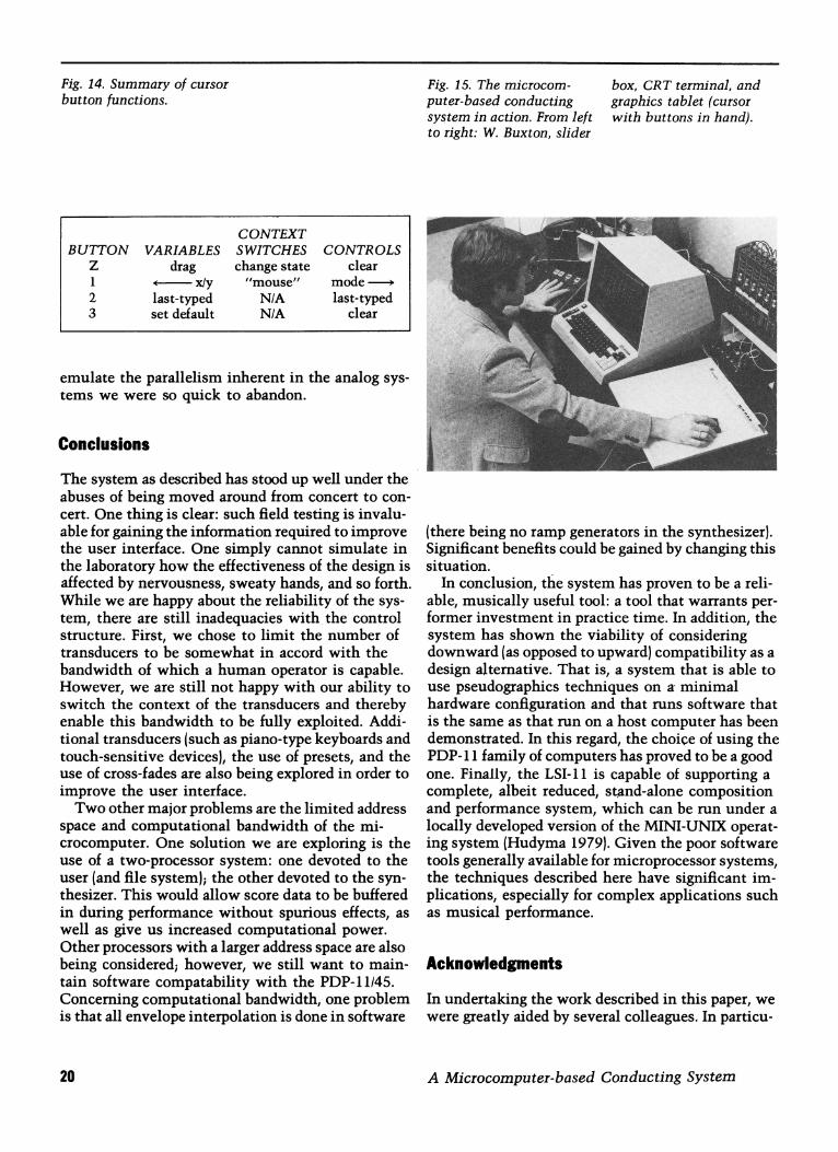
Fig. 14. Summary of cursor button functions.

CONTEXT BUTTON VARIABLES SWITCHES CONTROLS

Z drag change state clear 1 -- x/y "mouse" mode 2 last-typed N/A last-typed 3 set default N/A clear

Fig. 15. The microcomputer-based conducting system in action. From left to right: W. Buxton, slider

box, CRT terminal, and graphics tablet (cursor with buttons in hand).

. . .

..

. ..

.....++ "+

? .. .. .......

emulate the parallelism inherent in the analog systems we were so quick to abandon.

Conclusions The system as described has stood up well under the abuses of being moved around from concert to concert. One thing is clear: such field testing is invalu- able for gaining the information required to improve the user interface. One simply cannot simulate in the laboratory how the effectiveness of the design is affected by nervousness, sweaty hands, and so forth. While we are happy about the reliability of the system, there are still inadequacies with the control structure. First, we chose to limit the number of transducers to be somewhat in accord with the bandwidth of which a human operator is capable. However, we are still not happy with our ability to switch the context of the transducers and thereby enable this bandwidth to be fully exploited. Addi- tional transducers (such as piano-type keyboards and touch-sensitive devices), the use of presets, and the use of cross-fades are also being explored in order to improve the user interface.

Two other major problems are the limited address space and computational bandwidth of the microcomputer. One solution we are exploring is the use of a two-processor system: one devoted to the user (and file system); the other devoted to the synthesizer. This would allow score data to be buffered in during performance without spurious effects, as well as give us increased computational power. Other processors with a larger address space are also being considered; however, we still want to main- tain software compatability with the PDP-11/45. Concerning computational bandwidth, one problem is that all envelope interpolation is done in software

(there being no ramp generators in the synthesizer). Significant benefits could be gained by changing this situation.

In conclusion, the system has proven to be a reli- able, musically useful tool: a tool that warrants performer investment in practice time. In addition, the system has shown the viability of considering downward (as opposed to upward) compatibility as a design alternative. That is, a system that is able to use pseudographics techniques on a minimal hardware configuration and that runs software that is the same as that run on a host computer has been demonstrated. In this regard, the choice of using the PDP-11 family of computers has proved to be a good one. Finally, the LSI-11 is capable of supporting a complete, albeit reduced, stand-alone composition and performance system, which can be run under a locally developed version of the MINI-UNIX operat- ing system (Hudyma 1979). Given the poor software tools generally available for microprocessor systems, the techniques described here have significant im- plications, especially for complex applications such as musical performance.

Acknowledgments In undertaking the work described in this paper, we were greatly aided by several colleagues. In particu-


lar, we are grateful for the help provided by Michael Tilson, Robert Pike, Sanand Patel, and Thomas O'Dell in implementing some of the software. In addition, we would like to acknowledge the support of the Computer Systems Research Group Data Base project, especially Dennis Tsichritzis and Robert Hudyma. The cooperative environment that per- vades the Computer Systems Research Group has made the undertaking of this work a joy.

The research reported in this paper has been undertaken as part of the SSSP of the University of Toronto. This research is supported by the Social Sciences and Humanities Research Council of Canada. This support is gratefully acknowledged.

References 1. Alles, H. G. 1978. A portable digital sound synthesis

system. Computer Music Journal 1(4):5-6. 2. Arfib, D. 1978. Digital synthesis of complex spectra

by means of multiplication of non-linear distorted sine waves. AES Preprint No. 1319 (C-2).

3. Bartlett, M. 1979. Microcomputer-controlled synthesis system for live performance. Computer Music Journal 3(1):25-29.

4. Battier, M., and Arveiller, J. 1978. Documents musique et informatique: une bibliographie indexB. Elmeratto, Ivry S/Seine.

5. Buchla and Associates. 1978. User's guide to PATCH IV and the Series 300 Electric Music Box. Berkeley: Buchla and Associates.

6. Buxton, W., ed. 1977. Computer music 1976/77: a directory to current work. Ottawa: The Canadian Commission for UNESCO.

7. Buxton, W.; Fogels, E. A.; Fedorkow, G.; and Smith, K. C. 1978. An introduction to the SSSP Digital Syn- thesizer. Computer Music Journal 2(4):28-38.

8. Buxton, W.; Reeves, W.; Baecker, R.; and Mezei, L. 1978. The use of hierarchy and instance in a data structure for computer music. Computer Music Jour- nal, 2(4):10-20.

9. Buxton, W.; Reeves, W.; Fedorkow, G.; Smith, K. C., and Baecker, R. 1979. A computer-based system for the performance of electroacoustic music. AES Pre- print 1529 (J-1).

10. Buxton, W.; Sniderman, R.; Reeves, W.; Patel, S.; and Baecker, R. 1979. The evolution of the SSSP score editing tools. Computer Music Journal 3(4):14-25.

11. Chomsky, N. 1972. Syntactic structures, The Hague: Mouton.

12. Chowning, J. 1973. The synthesis of complex audio spectra by means of frequency modulation. J. Audio Eng. Soc., 21:526-534, and Computer Music Journal 1(2), 1977.

13. Cross, L. M. 1976. A bibliography of electronic music, Toronto: University of Toronto Press.

14. Davies, H. 1968. International electronic music catalog, Cambridge, Massachusetts: The MIT Press.

15. DEC. 1973. PDP-11/45 processor handbook. Maynard, Massachusetts: Digital Equipment Corp.

16. DEC. 1976. Microcomputer handbook. Maynard, Massachusetts: Digital Equipment Corp.

17. Hudyma, R. 1979. Mini-UNIX on the LSI-11. Paper presented at the UNIX Users Group Meeting, June 1979, University of Toronto, Toronto, Canada.

18. Kaegi, W., and Tempelaars, S. 1978. VOSIM-A new sound synthesis system. J. Audio Eng. Soc. 26:418- 424.

19. Kernighan, B., and Ritchie, D. 1978. The C programming language. Englewood Cliffs, New Jersey: Prentice-Hall.

20. Kobrin, E. 1975. HYBRID IV user's manual, La Jolla: C.M.E., U.C.S.D.

21. Le Brun, M. 1978. Digital waveshaping synthesis J. Audio Eng. Soc., 27:250-266.

22. Mathews, M. V. 1976. The Conductor Program. Paper presented at the First International Conference on Computer Music, October 1976, at MIT, Cambridge, Massachusetts.

23. Melby, J. 1976. Computer music compositions of the United States 1976. Beverly Hills, California:Theodore Front.

24. Moog, R. A. 1965. Voltage controlled electronic music modules. J. Audio Eng. Soc. 13:200.

25. Moorer, J. A. 1977. Signal processing aspects of computer music-a survey. Proceedings of the IEEE, 65:1108-1137.

26. New England Digital. 1978. Synclavier instruction manual. Norwich, Vermont: New England Digital Corporation.

27. Reeves, W.; Buxton, W.; Pike, R.; and Baecker, R. 1978. Ludwig: an example of interactive computer graphics in a score editor. Proceedings of the 1978 International Computer Music Conference, ed. C. Roads, 2: 392-409.

28. Ritchie, D., and Thompson, K. 1974. The UNIX time-sharing system. Communications of the ACM 17:365-375.


A Microcomputer-Based Conducting Systempagiamt/kcsmith/...baecker-conducting-system.pdf · based...

Documents

Transcript of A Microcomputer-Based Conducting Systempagiamt/kcsmith/...baecker-conducting-system.pdf · based...