A Methodology to Map Roughness Length and … · HARMONIE data interpolation in the FE domain: §...

University Institute for Intelligent Systems and Numerical Applications in Engineering

http://www.siani.es/

ESCO 2016 – 5th European Seminar on ComputingJune 5 - 10, 2016, Pilsen

A Methodology to Map Roughness Length and Displacement Height in Complex Terrain

Gustavo Montero, Eduardo Rodríguez, Albert Oliver, Guillermo V. Socorro-Marrero

Javier Calvo

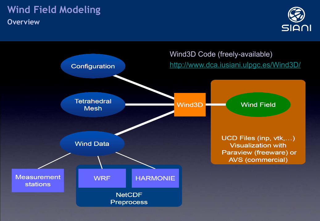
Wind Field ModelingOverview

Wind3D Code (freely-available)http://www.dca.iusiani.ulpgc.es/Wind3D/

Wind Field ModelingMass Consistent Wind Model

Let state the least square problem:

Objective:Find the velocity field

that adjusts to verifying:

Incompressibility condition in the domain andNo flow-through condition on the terrain

3RΩ⊂r · ~u = 0 in ⌦

~n · ~u = 0 on �b


Gauss Precision Moduli

They allow horizontal (α1) and vertical (α2) adjustment of wind velocity components

α >> 1 adjustment in vertical direction is predominant

α << 1 adjustment in horizontal direction is predominant

αè ∞ pure vertical adjustment

αè 0 pure horizontal adjustment


on

on

in

If Gauss Precision Moduli are constant,

SIMULACIN NUMRICA DE CAMPOS DE VIENTO 3

“Encontrar ~v 2 K tal que,

E(~v) = mın~u2K

E(~u), K =n

~u; ~r · ~u = 0, ~n · ~u|�b

= 0o

” (0.5)

Este problema es equivalente a encontrar el punto silla (~v, �) del Lagrangiano [?],

L(~u, �) = E(~u) +

Z

⌦

�

~r · ~u d⌦ (0.6)

La tcnica de los multiplicadores de Lagrange permite obtener el punto silla de la expresin (0.6),L(~v, �) L(~v, �) L(~u, �), tal que el campo solucin ~v se obtiene a partir de las ecuacionesde Euler-Lagrange,

~v = ~v

0

+ T

~r� (0.7)

siendo � el multiplicador de Lagrange y T = (Th

, T

h

, T

v

) el tensor diagonal de transmisin

T

h

=1

2↵2

1

, T

v

=1

2↵2

2

yT

v

T

h

= ↵

2 (0.8)

Si ↵

1

y ↵

2

se consideran constantes en todo el dominio, la formulacin variacional conduce auna ecuacin elptica definida en �. En efecto, sustituyendo la ecuacin (0.7) en (0.1) resulta

�~r · (T ~r�) = ~r · ~v0

(0.9)

que se completa con la condicin de Dirichlet nula en las fronteras permeables (fronterasverticales del dominio)

� = 0 en �a

(0.10)

y una condicin de Neumann en las impermeables (terreno y frontera superior)

~n · T

~r� = �~n · ~v0

en �b

(0.11)

Obsrvese que en la frontera superior, al ser el campo inicial ~v

0

horizontal, la condicin (0.11) setransforma en

~n · T

~r� = 0 (0.12)

Al considerar T

h

y T

v

constantes, la ecuacin (0.9) se convierte en

@

2

�

@x

2

+@

2

�

@y

2

+ ↵

2

@

2

�

@z

2

= � 1

T

h

✓

@u

0

@x

+@v

0

@y

+@w

0

@z

◆

(0.13)

0.1.2. Construccin del campo inicialPara la construccin del campo inicial partimos de los valores de la velocidad del viento y

de su direccin obtenidos en las estaciones de medida. El campo inicial ~v

0

se construye en tresetapas. En primer lugar, se calcula mediante interpolacin horizontal el valor de ~v

0

en los puntosdel dominio situados a la misma altura z

s

(sobre el terreno) que las estaciones de medida. Conesta informacin se realiza una extrapolacin vertical para definir el campo de velocidades entodo el dominio. Finalmente, la componente vertical del campo de velocidades es corregida enel entorno de posibles fuentes de emisin de contaminantes (chimeneas) con el fin de simular elmovimiento de salida de los gases.

Copyright c� 2005 U.L.P.G.C. IUSIANI Informe GANA-DDA-05-002Preparado con iusianirepe.cls

Once the Lagrange Multiplier is obtained, the wind velocity is computed with the Euler-Lagrange equations,

Construction of the observed windHorizontal interpolation



terrain surface

Vertical extrapolation (log-linear wind profile)

geostrophic wind

mixing layer

~u0(z) =~u⇤

k(log

z � d

z0� �m) k = 0.4

~ug

~u0(z) = ⇢(z) ~u0(zsl + d) + [1� ⇢(z)] ~ug

zpbl + d

zsl + d

z0 + d

z0

d

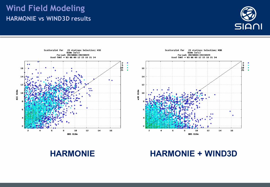
Wind Field ModelingHARMONIE vs WIND3D results

HARMONIE HARMONIE + WIND3D

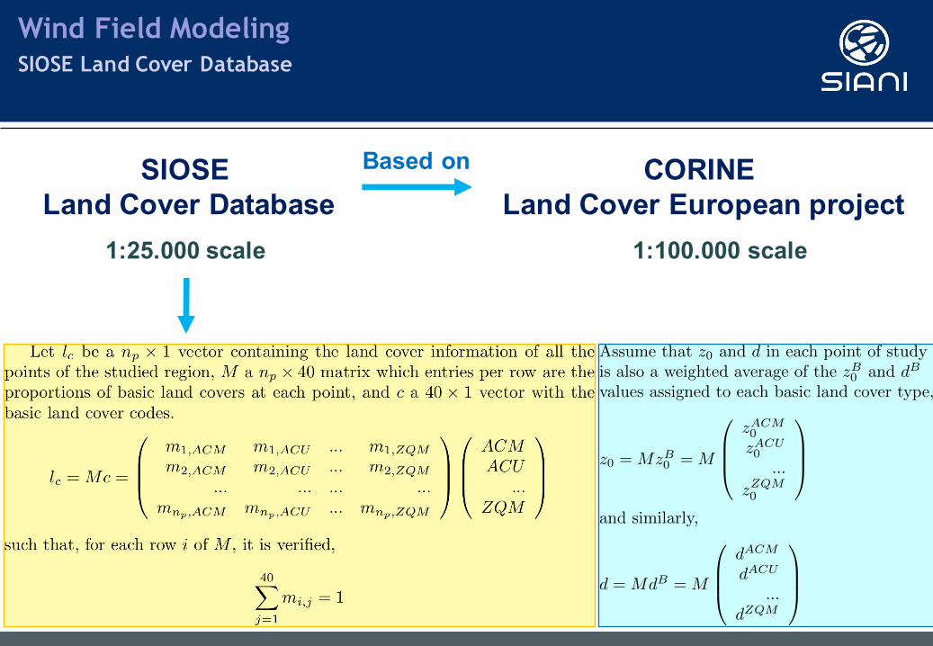
Wind Field ModelingSIOSE Land Cover Database

Assume that z0 and d in each point of study

is also a weighted average of the zB0 and dB

values assigned to each basic land cover type,

z0 = MzB0 = M

0

BB@

zACM0

zACU0

...zZQM0

1

CCA

and similarly,

d = MdB = M

0

BB@

dACM

dACU

...dZQM

1

CCA

SIOSE Land Cover Database

CORINE Land Cover European project

Based on

1:100.000 scale1:25.000 scale

Wind Field ModelingSIOSE Land Cover z0 and d

Wind Field ModelingPolygons of SIOSE Land Cover

SIOSE land cover polygons in the Island of Gran Canaria

SIOSE Land Cover

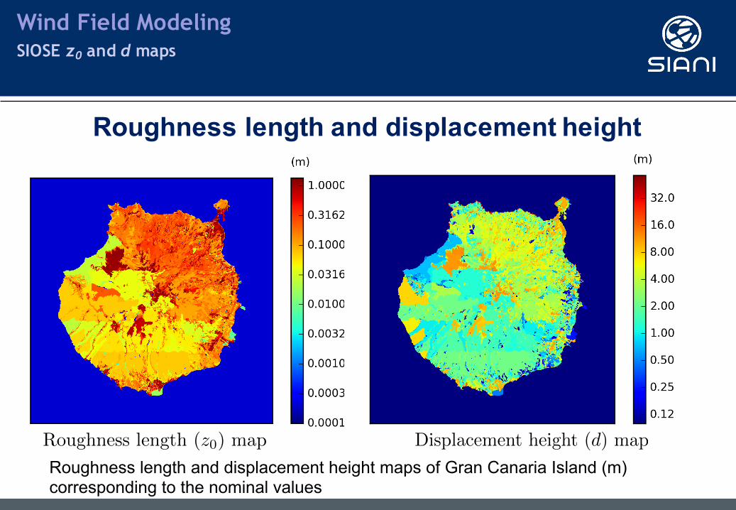
Wind Field ModelingSIOSE z0 and d maps

Roughness length and displacement height

Roughness length and displacement height maps of Gran Canaria Island (m) corresponding to the nominal values

Roughness length (z0) map Displacement height (d) map

Differential Evolution

Wind Field ModelingEstimation of Model Parameters

RMSE =

vuut 1

nc

ncX

i=1

(uxi

� uc

xi

)2 + (uyi

� uc

yi

)2 + (uzi

� uc

zi

)2

FE solutionis needed

for each individual

Rebirth:Differential Evolution

Reduction the search space:Student T distribution

L-BFGS-B

NE times

Wind Field ModelingHARMONIE-FEM wind forecast

Wind Field ModelingHARMONIE-FEM wind forecast

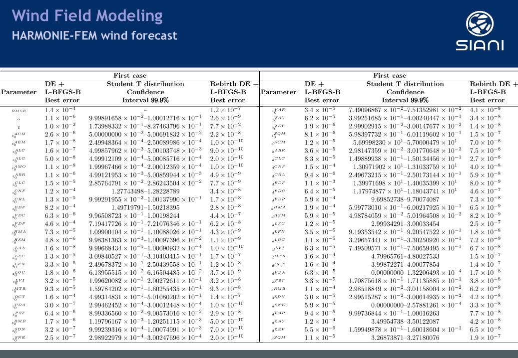
First case

DE + Student T distribution Rebirth DE +

Parameter L-BFGS-B Confidence L-BFGS-B

Best error Interval 99.9%99.9%99.9% Best error

RMSE 1.4⇥ 10�4 – 1.2⇥ 10�7

↵ 1.1⇥ 10�6 9.99891658⇥ 10�2–1.00012716⇥ 10�1 2.6⇥ 10�9

⇠ 1.0⇥ 10�2 1.73988332⇥ 10�1–8.27463796⇥ 10�1 7.7⇥ 10�2

zACM0 2.6⇥ 10�6 5.00000000⇥ 10�2–5.00691832⇥ 10�2 2.2⇥ 10�8

zAEM0 1.7⇥ 10�8 2.49948364⇥ 10�4–2.50089986⇥ 10�4 1.0⇥ 10�10

zALC0 1.6⇥ 10�7 4.99857962⇥ 10�3–5.00103748⇥ 10�3 9.0⇥ 10�10

zALG0 5.0⇥ 10�8 4.99912109⇥ 10�4–5.00085716⇥ 10�4 2.0⇥ 10�10

zAMO0 1.1⇥ 10�8 1.99967466⇥ 10�4–2.00012359⇥ 10�4 1.0⇥ 10�10

zARR0 1.1⇥ 10�6 4.99121953⇥ 10�3–5.00859944⇥ 10�3 4.9⇥ 10�9

zCLC0 1.5⇥ 10�5 2.85764791⇥ 10�2–2.86243504⇥ 10�2 7.7⇥ 10�9

zCNF0 1.2⇥ 10�4 1.27743498–1.28228789 3.4⇥ 10�8

zCHL0 1.3⇥ 10�5 9.99291955⇥ 10�2–1.00137990⇥ 10�1 1.7⇥ 10�8

zEDF0 8.2⇥ 10�4 1.49719791–1.50218395 2.8⇥ 10�8

zFDC0 6.3⇥ 10�6 9.96508723⇥ 10�1–1.00198244 4.4⇥ 10�7

zFDP0 4.6⇥ 10�4 7.19417726⇥ 10�1–7.21076346⇥ 10�1 6.2⇥ 10�8

zHMA0 7.3⇥ 10�5 1.09900104⇥ 10�1–1.10088026⇥ 10�1 4.3⇥ 10�9

zHSM0 4.8⇥ 10�6 9.98381363⇥ 10�3–1.00097396⇥ 10�2 1.1⇥ 10�9

zLAA0 1.6⇥ 10�8 9.99668434⇥ 10�5–1.00090932⇥ 10�4 1.0⇥ 10�10

zLFC0 1.3⇥ 10�5 3.09840527⇥ 10�1–3.10403415⇥ 10�1 1.7⇥ 10�7

zLFN0 3.3⇥ 10�5 2.49678372⇥ 10�1–2.50439558⇥ 10�1 1.2⇥ 10�8

zLOC0 1.8⇥ 10�6 6.13955515⇥ 10�2–6.16504485⇥ 10�2 3.7⇥ 10�9

zLV I0 3.2⇥ 10�5 1.99620082⇥ 10�1–2.00272611⇥ 10�1 3.2⇥ 10�8

zMTR0 9.3⇥ 10�5 1.59784202⇥ 10�1–1.60255435⇥ 10�1 9.3⇥ 10�8

zOCT0 1.6⇥ 10�4 4.99314831⇥ 10�1–5.01080202⇥ 10�1 1.4⇥ 10�7

zPDA0 3.0⇥ 10�7 2.99462452⇥ 10�4–3.00012448⇥ 10�4 1.0⇥ 10�10

zPST0 6.4⇥ 10�6 8.99336560⇥ 10�2–9.00573016⇥ 10�2 2.9⇥ 10�8

zRMB0 1.7⇥ 10�6 1.19796167⇥ 10�3–1.20251115⇥ 10�3 5.0⇥ 10�10

zSDN0 3.2⇥ 10�7 9.99239316⇥ 10�4–1.00074991⇥ 10�3 7.0⇥ 10�10

zSNE0 2.5⇥ 10�7 2.98922979⇥ 10�4–3.00247696⇥ 10�4 2.0⇥ 10�10

First case

DE + Student T distribution Rebirth DE +

Parameter L-BFGS-B Confidence L-BFGS-B

Best error Interval 99.9%99.9%99.9% Best error

zV AP0 3.4⇥ 10�5 7.49096867⇥ 10�2–7.51352981⇥ 10�2 4.1⇥ 10�8

zZAU0 6.2⇥ 10�5 3.99251685⇥ 10�1–4.00240447⇥ 10�1 3.4⇥ 10�8

zZEV0 1.9⇥ 10�6 2.99902915⇥ 10�2–3.00147677⇥ 10�2 1.4⇥ 10�8

zZQM0 8.1⇥ 10�6 5.98397732⇥ 10�1–6.01119602⇥ 10�1 1.5⇥ 10�7

dACM 1.2⇥ 10�5 5.69998230⇥ 101–5.70000479⇥ 101 7.0⇥ 10�8

dARR 3.6⇥ 10�5 2.98147359⇥ 10�2–3.01770648⇥ 10�2 7.5⇥ 10�8

dCLC 8.3⇥ 10�5 1.49889938⇥ 10�1–1.50134456⇥ 10�1 2.7⇥ 10�8

dCNF 1.5⇥ 10�4 1.30971902⇥ 101–1.31033759⇥ 101 4.0⇥ 10�8

dCHL 9.4⇥ 10�6 2.49673215⇥ 10�1–2.50173144⇥ 10�1 5.9⇥ 10�8

dEDF 1.1⇥ 10�3 1.39971698⇥ 101–1.40035399⇥ 101 8.0⇥ 10�9

dFDC 6.4⇥ 10�5 1.17974877⇥ 101–1.18043741⇥ 101 4.6⇥ 10�7

dFDP 5.9⇥ 10�4 9.69852738–9.70074087 7.3⇥ 10�8

dHMA 1.9⇥ 10�4 5.99773010⇥ 10�1–6.00217925⇥ 10�1 6.5⇥ 10�9

dHSM 5.9⇥ 10�5 4.98784059⇥ 10�2–5.01964508⇥ 10�2 8.2⇥ 10�9

dLFC 1.2⇥ 10�5 2.99934291–3.00033454 2.5⇥ 10�7

dLFN 3.5⇥ 10�5 9.19353542⇥ 10�1–9.20547522⇥ 10�1 1.8⇥ 10�8

dLOC 1.1⇥ 10�5 3.29657441⇥ 10�1–3.30250920⇥ 10�1 7.2⇥ 10�9

dLV I 6.3⇥ 10�5 7.49509571⇥ 10�1–7.50659495⇥ 10�1 6.7⇥ 10�8

dMTR 1.6⇥ 10�4 4.79965761–4.80027533 1.5⇥ 10�7

dOCT 1.6⇥ 10�4 3.99872271–4.00077854 1.4⇥ 10�7

dPDA 6.3⇥ 10�5 0.00000000–1.32206493⇥ 10�4 1.7⇥ 10�8

dPST 3.3⇥ 10�5 1.70875618⇥ 10�1–1.71135885⇥ 10�1 3.8⇥ 10�8

dRMB 1.1⇥ 10�4 2.98518849⇥ 10�2–3.01158004⇥ 10�2 6.2⇥ 10�9

dSDN 3.0⇥ 10�5 2.99515287⇥ 10�2–3.00614935⇥ 10�2 4.2⇥ 10�8

dSNE 5.9⇥ 10�5 0.00000000–2.57881261⇥ 10�4 3.3⇥ 10�8

dV AP 9.4⇥ 10�5 9.99736844⇥ 10�1–1.00016263 7.7⇥ 10�8

dZAU 1.2⇥ 10�4 3.49954738–3.50122087 4.2⇥ 10�8

dZEV 5.5⇥ 10�6 1.59949878⇥ 10�1–1.60018604⇥ 10�1 6.5⇥ 10�8

dZQM 1.1⇥ 10�5 3.26873871–3.27180076 1.9⇥ 10�7

Wind Field ModelingSummer wind rose of Gran Canaria

Wind Rose of Gran Canaria at 10m relating to the period from June 1 to

September 30 of the year 2015.

Daytime Nighttime

Wind Field ModelingSelected cases

Cases DaytimeSurface Surface HARMONIE HARMONIE Incoming Pasquillwind wind speed 10 m wind 10 m wind solar stability

direction range (m/s) speed direction radiation class

NNE > 6 7,61 32,89 530,85 D

NE > 6 9,01 37,29 583,39 D

N > 6 7,11 349,53 494,75 D

NE 5� 6 5,57 40,50 665,60 C

N 3� 5 4,16 4,26 797,14 B

NNE 5� 6 5,88 12,76 771,82 C

NNE 3� 5 3,54 12,70 586,43 C

N 5� 6 5,39 350,28 695,26 C

Cases NighttimeSurface Surface HARMONIE HARMONIE Cloud Pasquillwind wind speed 10 m wind 10 m wind amount stability

direction range (m/s) speed direction (oktas) class

NNE > 6 9,87 25,75 4,59 D

NE > 6 8,07 34,16 3,39 D

N > 6 6,82 355,35 7,04 D

NE 5� 6 5,10 42,58 2,24 D

N 3� 5 4,99 359,27 6,45 D

NNE 5� 6 5,13 19,94 0,61 D

NNE 3� 5 4,90 12,56 0,00 E

N 5� 6 5,62 353,72 1,86 D

Table 1: Most frequent wind speeds and directions in the island of Gran Canaria

during the summer months.

0,0019-0,0043

0,00-0,00

Wind Field ModelingMeasurement stations

Code Name x (m)x (m)x (m) y (m)y (m)

y (m) z (m)z (m)z (m)

C611E Vega de San Mateo 442587.00 3094849.87 1712C612F Cruz de Tejeda 441111.20 3098128.27 1524C619I La Aldea de San Nicolas 420071.67 3097617.70 20C619X Agaete 429982.92 3108624.01 15C619Y La Aldea 420598.02 3097574.90 23C623I S. Bartolome de Tirajana, Cuevas del Pinar 440978.20 3089240.95 1230C625O S. Bartolome de Tirajana, Lomo Pedro Alfonso 436499.77 3081522.42 816C628B La Aldea de San Nicolas, Tasarte 424210.25 3087335.04 328C629I Mogan, Puerto 424469.50 3077087.00 22C629Q Mogan, Puerto Rico 429927.60 3073056.56 20C629X Puerto de Mogan 424751.35 3077101.81 20C639M Maspalomas, C. Insular Turismo 443238.31 3070506.07 55C639U S. Bartolome de Tirajana, El Matorral 455345.47 3076502.74 51C648C Aguimes 455325.70 3086483.97 316C648N Telde, Centro Forestal Doramas 454970.89 3095890.75 354C649I Gran Canaria, Aeropuerto 461658.52 3088640.43 34C649R Telde, Melenara 462854.84 3095804.64 19C656V Teror 446227.23 3105674.70 693C659H Polıgono de San Cristobal 459130.00 3107201.82 65C659M Plaza de la Feria 458627.05 3109809.55 25C665T Valleseco 444392.38 3104643.66 910C669B Arucas 450225.76 3113015.52 96C689E Maspalomas 441057.23 3068075.14 35

Location in UTM zone 28N coordinates and height over the sea level of the 23anemometers available in Gran Canaria.

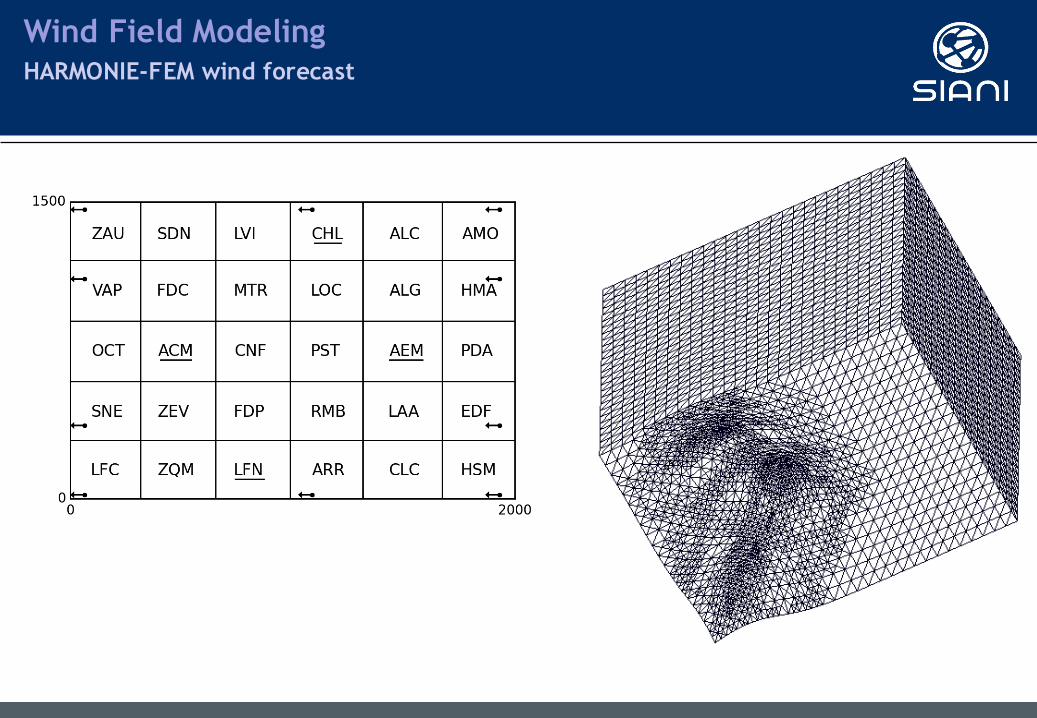
Wind Field ModelingAdaptive mesh

Surface triangulation

Domain dimensions: 76 km ✕ 85 km ✕ 4 km

1.492.804 tetrahedra326.101 nodes

Local refinement:- Measurement stations- Shoreline- Altimetry

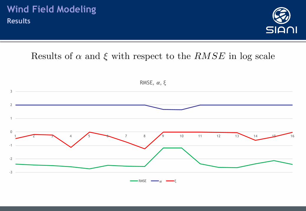
Wind Field ModelingResults

Results of ↵ and ⇠ with respect to the RMSE in log scale

-3

-2

-1

0

1

2

3

1 2 3 4 5 6 7 8 9 10 11 12 13 14 15 16

RMSE, 𝜶, ξ

RMSE 𝜶 ξ


5-6 m/s NNE C 3-5 m/s NNE E

Roughness length (z0) map


Displacement height (d) map

>6 m/s NNE D 5-6 m/s NNE D

Wind Field ModelingConclusions and Future Research

- Mass Consistent models (MCM) can improve the forecasting results of Mesoscale models

- The studied parameters involved in MCM depend on the wind velocity (speed and direction), and the atmospheric stability. Also daytime and nighttime results are different.

- The mimetic algorithm proposed is a robust tool for solving this type of parameter estimation problems.

- Construct a reduced basis of those parameters for solving wind episodes (different locations). Only forecasting values as input data.

- Apply this methodology to the results of different mesoscale models (HARMONIE, ECMWF)

Conclusions

Future Research

HARMONIE data interpolation in the FE domain:§ Use U10 and V10 supposing it is 10m over the FE surface + height displacement

HARMONIE FD domain WIND3D FE domain

Wind Field ModelingData interpolation in FE domain


Statement of the problemTo find such that,

with

of the Lagrangian

The solution produces the Euler-Lagrange equations

where

This is equivalent to find the saddle point


on

on

in

Substituting the Euler-Lagrange equation in,

on

in

it yields the governing equations,


h = �0r

|~u⇤| Lf

zpbl =� |~u⇤|f

● Friction velocity:

● Height of the planetary boundary layer:

the Earth rotation andis the Coriolis parameter, being

is a parameter depending on the atmospheric stability

is the latitude

● Mixing height:

in neutral and unstable conditions

in stable conditions

● Height of the surface layer:

Atmospheric Stratification

0.15 < γ < 0.45

γ’ ≅ 0.4

~u⇤=

k ~u0(zm)

log

zm � d

z0� �m

f = 2⌦ sin��

h = zpbl

zsl =h10

A Methodology to Map Roughness Length and … · HARMONIE data interpolation in the FE domain: §...

Documents

Transcript of A Methodology to Map Roughness Length and … · HARMONIE data interpolation in the FE domain: §...