A METHODOLOGY FOR ASSESSING THERMAL STRATIFICATION …

A METHODOLOGY FOR ASSESSING THERMAL STRATIFICATION IN AN

HCCI ENGINE AND UNDERSTANDING THE IMPACT OF ENGINE DESIGN

AND OPERATING CONDITIONS

by

Benjamin John Lawler

A dissertation submitted in partial fulfillment

of the requirements for the degree of

Doctor of Philosophy

(Mechanical Engineering)

in the University of Michigan

2013

Doctoral Committee:

Professor Arvind Atreya, Co-Chair

Professor Zoran Filipi, Co-Chair, Clemson University

Associate Professor Claus Borgnakke

Professor James Driscoll

Research Scientist George Lavoie

Professor Volker Sick

© Reserved Rights All

LawlerJohn Benjamin 2013

ii

To my Aunt Eileen Mahoney,

who was always proud of my accomplishments

iii

ACKNOWLEDGMENTS

There are a number of people whose contributions made this research possible.

First, I would like to thank my advisor, Professor Zoran Filipi, for the opportunity to do

this research and his guidance and support throughout my graduate career. I would also

like to thank Professor Arvind Atreya for joining the project and becoming Co-Chair

when Professor Filipi moved to Clemson University and for helping to ensure a

successful conclusion of the research. Similarly, Professor Claus Borgnakke’s assistance

during the later stages of the project and his valuable feedback helped the research reach

completion. Special thanks to Professor Volker Sick for giving me all the support he

could and making sure I had everything I needed to conduct this research. I would like to

thank Dr. George Lavoie for interacting with me on a more regular basis and helping to

validate the proposed analysis technique. Special thanks to Professor James Driscoll for

serving on my committee as the cognate member and providing his cross-departmental

perspective and feedback on this research.

In addition to the committee members, I would like to thank the researchers at

General Motors Research and Development for funding the test cell, providing the initial

motivation for the work, and offering invaluable feedback on a monthly basis.

Specifically, Paul Najt and Dr. Orgun Güralp were instrumental in directing and guiding

this project through our useful technical discussions. Other members of General Motors

Research and Development who contributed positively to this work were Dr. Han Ho, Dr.

Seunghwan Keum, and Dr. Ronald Grover. I would also like to thank Dr. John Dec, Dr.

Nicolas Dronniou, and Dr. Jeremie Dernotte at Sandia National Laboratories for

iv

collaborating to provide the optical data for validation and their feedback during our

meetings.

As well as the funding provided by General Motors for the test cell, I would like

to thank the Department of Mechanical Engineering at the University of Michigan for my

personal funding for a year through a departmental fellowship. Also, I would like to

thank the National Science Foundation Graduate Research Fellowship Program (Grant

No. DGE0718128) for my personal funding for three years.

Special thanks to all of my co-workers and colleagues in the Walter E. Lay

Automotive Laboratory at the University of Michigan. Specifically, I would like to thank

Professor Andre Boehman and Professor Volker Sick, who are patiently waiting for me to

graduate to inherit my test cell, but never made me feel rushed or like I over stayed my

welcome. Also, I would like to thank my colleagues Luke Hagen for all the help in the

test cell and Ashwin Salvi for the technical discussions, help in the test cell, and the

infrared imaging. This work would not have been possible without the help of Dr. Josh

Lacey, who contributed technically to the work with his feedback, helped run the engine

and collect data, and assisted in the test cell setting up the experimental capabilities. I

would also like to recognize the help and work of Satyum Joshi, who helped run the

engine and collect data and helped in the design and construction of the glow plug sleeve

adapters.

The staff of the Autolab is pivotal in managing all the work behind the scenes that

allows the student to conduct their research. Special thanks to Melissa McGeorge, Laurie

Stoianowski, and Kathie Wolney for all of their help placing orders, booking rooms, and

general help anytime I needed it. Also, I would like to thank Kent Pruss who made the

glow plug sleeve adapters and compression ratio spacers used in this research.

Finally, I would like to thank all my other co-workers, colleagues, friends, and

family, whose support made this work possible. Specifically I would like to thank my

v

supportive family who has always believed in me. Last but not least, I would like to

thank my loving girlfriend, who helped me in more ways than I can express.

vi

TABLE OF CONTENTS

DEDICATION....................................................................................................... ii

ACKNOWLEDGMENTS ................................................................................... iii

LIST OF FIGURES ............................................................................................. xi

LIST OF TABLES ............................................................................................. xix

LIST OF ACRONYMS ...................................................................................... xx

ABSTRACT ....................................................................................................... xxii

CHAPTER 1 INTRODUCTION, BACKGROUND, MOTIVATION, AND

OBJECTIVES ................................................................................................. 1

1.1 Introduction .................................................................................................. 1

1.2 Background .................................................................................................. 2

1.2.1 Homogeneous Charge Compression Ignition ........................................2

1.2.2 Thermal Characterization of HCCI ......................................................11

1.2.3 Optical Investigations: A New Understanding of HCCI .....................14

1.2.4 Computational Fluid Dynamics Research ...........................................23

1.3 Motivation and Objectives ......................................................................... 25

1.3.1 Motivation for the Current Study .........................................................25

1.3.2 Research Objectives .............................................................................26

CHAPTER 2 DEVELOPMENT OF THE THERMAL STRATIFICATION

ANALYSIS .................................................................................................... 28

2.1 Heat Release Analysis ................................................................................ 29

2.1.1 Time Averaged Data Processing ..........................................................29

2.1.2 Ensemble Averaging ............................................................................30

2.1.3 Pressure Filtering .................................................................................31

2.1.4 Pressure Pegging ..................................................................................32

vii

2.1.5 Trapped Mass and Bulk Temperature ..................................................32

2.1.6 Heat Transfer Correlation ....................................................................37

2.1.7 Heat Release Calculation .....................................................................38

2.2 Thermal Stratification Analysis Methodology ........................................... 39

2.2.1 Analysis of the Burned Mass ...............................................................40

2.2.2 Extension to the Unburned Mass .........................................................53

2.2.3 Removing the Normalization ...............................................................57

2.2.4 Thermal Width .....................................................................................63

2.2.5 Review of the TSA Assumptions .........................................................64

2.3 Sensitivity of the TSA to the Ignition Delay Correlation ........................... 65

2.3.1 Effect of Activation Energy .................................................................65

2.3.2 Effect of the Pre-exponential Constant in the Ignition Delay

Correlation ..............................................................................................68

2.3.3 Effect of the Negative Temperature Coefficient Region in the

Ignition Delay Correlation ......................................................................69

2.4 Chapter Summary ....................................................................................... 75

CHAPTER 3 VALIDATION OF THE THERMAL STRATIFICATION

ANALYSIS .................................................................................................... 77

3.1 Validation against Computational Fluid Dynamics Simulations ............... 77

3.2 Validation against Optically Measured Data .............................................. 83

3.3 Chapter Summary ....................................................................................... 92

CHAPTER 4 TEST CELL DESCRIPTION .................................................... 94

4.1 Default Test Cell Configuration ................................................................. 94

4.1.1 Engine ..................................................................................................95

4.1.2 Fuel Type .............................................................................................97

4.1.3 Dynamometer .......................................................................................98

viii

4.1.4 Emissions Measurements .....................................................................98

4.2 Instrumentation ......................................................................................... 100

4.2.1 Pressure Measurements ......................................................................100

4.2.2 Heat Flux Probes ................................................................................100

4.2.3 Crank Angle Resolved Data Acquisition ...........................................102

4.2.4 Time Averaged Data Acquisition ......................................................102

4.3 Experimental Capabilities ........................................................................ 104

4.3.1 Intake Heating ....................................................................................104

4.3.2 Direct Injection versus Fully Premixed Fuel Delivery ......................105

4.3.3 Rebreathe versus Positive Valve Overlap Operation .........................106

4.4 Thermal Images of the Test Cell .............................................................. 108

CHAPTER 5 EFFECT OF OPERATING CONDITIONS ON THERMAL

STRATIFICATION .................................................................................... 113

5.1 Fuel Preparation ....................................................................................... 114

5.1.1 Direct Injection versus Fully Premixed Fuel Delivery ......................115

5.1.2 Injection Timing Sweep .....................................................................118

5.2 Internal Residual Dilution versus Air Dilution ........................................ 122

5.3 Intake Temperature Sweep ....................................................................... 130

5.4 Premixed Positive Valve Overlap Combustion Phasing Study ................ 134

5.5 Positive Valve Overlap Swirl Study ......................................................... 142

5.6 Premixed Positive Valve Overlap Compensated Load Sweep ................. 149

5.7 Chapter Summary ..................................................................................... 153

CHAPTER 6 EFFECT OF WALL CONDITIONS ON THERMAL

STRATIFICATION .................................................................................... 154

6.1 Wall Temperature ..................................................................................... 154

6.2 Ceramic Coatings ..................................................................................... 161

6.3 Chapter Summary ..................................................................................... 166

ix

CHAPTER 7 EFFECT OF ENGINE GEOMETRY ON THERMAL

STRATIFICATION .................................................................................... 167

7.1 Compression Ratio ................................................................................... 168

7.2 Piston Geometry ....................................................................................... 172

7.3 Chapter Summary ..................................................................................... 177

CHAPTER 8 EFFECT OF A GLOW PLUG ON HCCI COMBUSTION.. 179

8.1 Design, Construction, and Glow Plug Tip Temperature .......................... 180

8.1.1 Side Mounted Configuration..............................................................180

8.1.2 Centrally Mounted Configuration ......................................................183

8.1.3 Glow Plug Tip Temperature ..............................................................184

8.2 Baseline Conditions .................................................................................. 187

8.2.1 Combustion Phasing ..........................................................................187

8.2.2 Temperature Distributions and Thermal Width .................................188

8.2.3 Indicated Efficiency ...........................................................................193

8.3 Lower Engine Speed Operation ............................................................... 195

8.3.1 Combustion Phasing and Temperature Distributions ........................195

8.3.2 Efficiency and Emissions ...................................................................200

8.4 Centrally Mounted Glow Plug ................................................................. 204

8.5 Glow Plug with Swirl ............................................................................... 206

8.6 Chapter Summary ..................................................................................... 209

CHAPTER 9 CONCLUSIONS, SCIENTIFIC CONTRIBUTIONS, AND

RECOMMENDATIONS FOR FUTURE WORK ................................... 211

9.1 Summary and Conclusions ....................................................................... 211

9.2 Scientific Contributions ............................................................................ 215

9.2.1 Characterization of the Impact of Design and Operating

Conditions .............................................................................................216

9.2.2 Control of Thermal Stratification with a Glow Plug .........................218

x

9.3 Recommendations for Future Work ......................................................... 218

REFERENCES .................................................................................................. 220

xi

LIST OF FIGURES

Figure 1.1 − Graphic comparison of the three types of combustion modes [7].................. 4

Figure 1.2 − a) Comparison of the HCCI operating range to the SI operating range

and b) engine operating points over EPA UDDS [35, 36] ...........................................9

Figure 1.3 − a) Experimentally measured heat flux and b) heat flux predicted by

the Chang heat transfer correlation over three speed settings [37] ............................12

Figure 1.4 − Example of the advanced combustion phasing and accelerated burn

rates of HCCI combustion with higher wall temperatures [38] .................................13

Figure 1.5 − Effect of deposit growth on HCCI combustion heat release rates [39] ........ 14

Figure 1.6 − Chemiluminescence images of HCCI combustion taken by John Dec

at Sandia National Laboratories [14] .........................................................................15

Figure 1.7 − Sequential chemiluminescence images of HCCI combustion [14] .............. 16

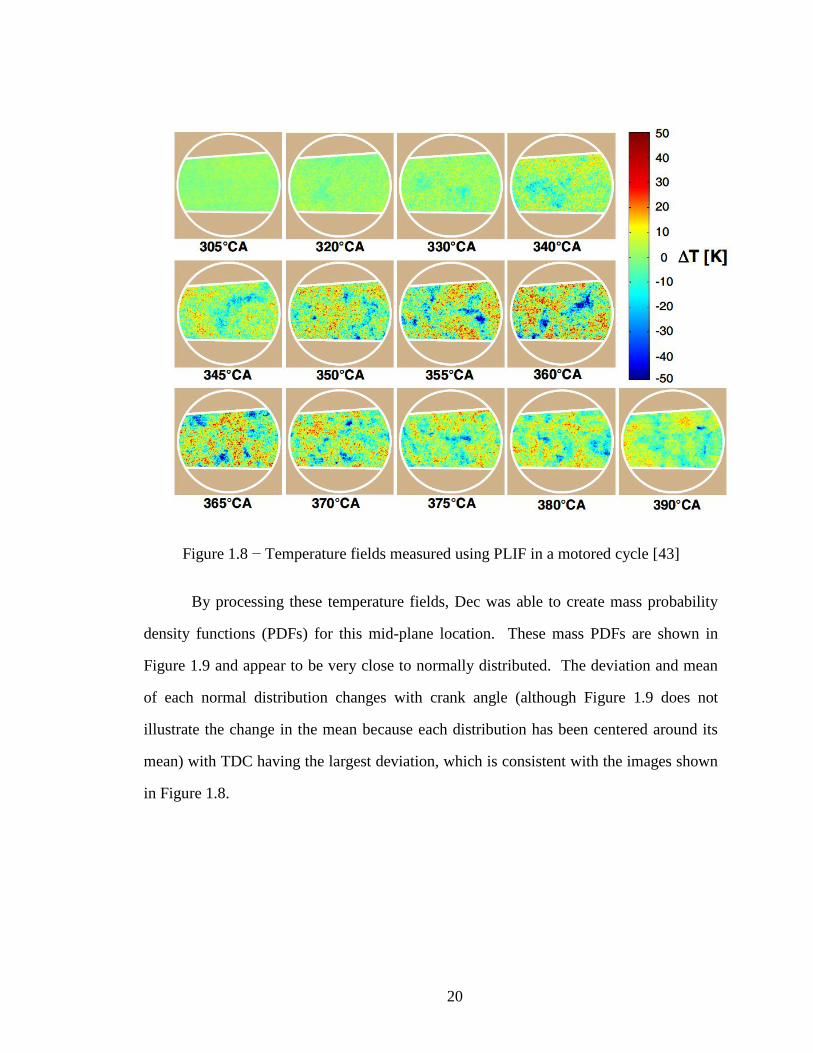
Figure 1.8 − Temperature fields measured using PLIF in a motored cycle [43] .............. 20

Figure 1.9 − Unburned temperature distributions at the mid-plane of the cylinder

derived from the measured temperature fields [43] ...................................................21

Figure 1.10 − Optically measured temperature field in a vertical plane [45] ................... 22

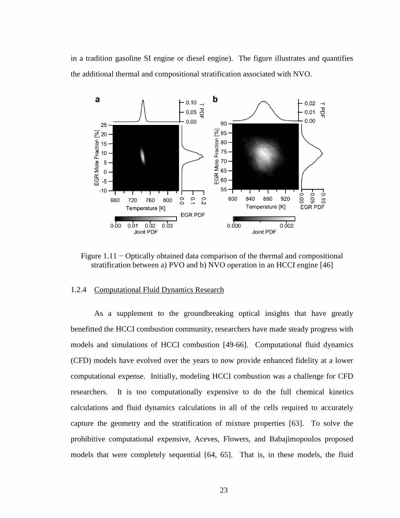
Figure 1.11 − Optically obtained data comparison of the thermal and

compositional stratification between a) PVO and b) NVO operation in an

HCCI engine [46] .......................................................................................................23

Figure 2.1 − Graphic illustration of the cylinder and its contents at IVC for

determining the mass of the internal residuals ...........................................................34

Figure 2.2 − Measured cylinder pressure for the baseline operating conditions ...............42

Figure 2.3 − Bulk and isentropic unburned temperature comparison ................................43

xii

Figure 2.4 − Temperature profiles for varying NZT and their respective ignition

timings predicted by the autoignition integral ...........................................................46

Figure 2.5 − a) Ignition phasing versus normalized temperature, b) mass fraction

burned curve, and c) NZT-MFB curve ......................................................................51

Figure 2.6 − Cumulative distribution function and probability density function ..............53

Figure 2.7 − Mass PDF with exponential fit for the unburned and discarded part ............55

Figure 2.8 − Complete normalized temperature distribution .............................................56

Figure 2.9 − Isentropic temperature comparisons with the measured wall

temperature ................................................................................................................59

Figure 2.10 − Mass CDF and PDF versus absolute, unburned charge temperature ..........61

Figure 2.11 − Three dimensional surface plot of the unburned temperature

distribution over the compression and expansion processes ......................................62

Figure 2.12 − Effect of varying the activation energy in the ignition delay

correlation on the mass PDFs ....................................................................................67

Figure 2.13 − Effect of varying the pre-exponential constant in the ignition delay

correlation on the mass PDFs ....................................................................................69

Figure 2.14 − Comparison of the He and Goldsborough ignition delay correlations ........70

Figure 2.15 − Comparison of the He and the Goldsborough ignition delay

correlation showing the hybrid correlation for determining the effects of the

NTC region on the TSA results .................................................................................72

Figure 2.16 − Unburned temperature distributions calculated with the He

correlation and the hybrid He NTC correlation .........................................................73

Figure 2.17 − Contributions to the autoignition integral and 1000 over the

isentropic unburned temperature................................................................................74

Figure 2.18 − Effect of the NTC region on the mass PDFs for a low speed (800

rpm) point...................................................................................................................75

xiii

Figure 3.1 − Mass fraction burned curve for a single zone HCCI combustion

model at conditions representative of the experimental data .....................................79

Figure 3.2 − Mass fraction burned curves for the three CFD simulations used for

validation of the TSA .................................................................................................80

Figure 3.3 − Comparison between the known CFD distribution and the TSA-

determined distribution for (a) an early phased case, (b) a mid-phased case,

and (c) a retarded case with CA50 phasings at 5, 12.5, and 20.5 CA aTDC,

respectively ................................................................................................................82

Figure 3.4 − Illustration of the image volume weighting to create a cylinder-wide

distribution from a single plane temperature map [94] ..............................................85

Figure 3.5 − Comparison between the optically measured distributions and the

TSA-determined distributions at -40 CA, -20 CA, TDC, and 20 CA ........................88


TSA-determined distributions for the 60 °C coolant temperature data point at

TDC and 10 CA .........................................................................................................89


TSA-determined distributions for the 100 °C coolant temperature data point

at TDC and 10 CA .....................................................................................................90

Figure 4.1 − Graphic illustration of the test cell used in this research [37] .......................95

Figure 4.2 − Photograph of the head and piston geometries [100] ....................................96

Figure 4.3 − Horiba Mexa7100DEGR emission analyzer bench ......................................99

Figure 4.4 − Heat flux probe schematic [102] .................................................................101

Figure 4.5 − Default rebreathe valve lift profile .............................................................108

Figure 4.6 − a) Photograph and b) infrared thermal image of the test cell ......................110

Figure 4.7 − IR thermography of the engine while running ............................................112

xiv

Figure 5.1 − Unburned temperature distributions comparing direct injection

versus fully premixed operation...............................................................................117

Figure 5.2 − Mass fraction burned curves for the injection timing sweep ......................119

Figure 5.3 − 10% to 90% thermal width and 25% to 75% thermal width for the

injection timing sweep .............................................................................................120

Figure 5.4 − Net indicated fuel conversion efficiency, combustion efficiency,

NOx and CO emissions for the injection timing sweep ...........................................122

Figure 5.5 − Mass fraction burned curves for high and low residual gas fraction

comparison at 11 mg and 9 mg of fuel per cycle .....................................................125

Figure 5.6 − Unburned temperature distributions at TDC for high and low internal

residual gas fraction comparison at 9 mg and 11 mg of fuel per cycle ...................127

Figure 5.7 − 25% to 75% thermal widths for the internal residual gas fraction

study .........................................................................................................................128

Figure 5.8 − 10% to 90% thermal widths for the internal residual gas fraction

study .........................................................................................................................129

Figure 5.9 − Mass fraction burned curves for the intake temperature sweep ..................131

Figure 5.10 − Unburned temperature distributions for the intake temperature

sweep........................................................................................................................132

Figure 5.11 − Thermal widths for the intake temperature sweep ....................................133

Figure 5.12 − Mass fraction burned curves for an intake temperature sweep and an

equivalence ratio sweep under premixed conditions with the PVO camshafts .......136

Figure 5.13 − Unburned temperature distributions at TDC for an intake

temperature sweep and an equivalence ratio sweep under premixed

conditions with the PVO camshafts .........................................................................140

Figure 5.14 − Thermal widths for the equivalence ratio (Phi) and intake

temperature (Tint) sweeps plotted against combustion phasing ...............................142

xv

Figure 5.15 − Mass fraction burned curves for the PVO intake temperature

sweeps with and without swirl .................................................................................144

Figure 5.16 − Unburned temperature distributions with and without swirl for the

mid-phased condition ...............................................................................................145

Figure 5.17 − 10% to 90% and 25% to 75% thermal widths for the swirl study ............146

Figure 5.18 − Percent change of thermal width with the addition of swirl as a

function of combustion phasing ...............................................................................147

Figure 5.19 − Net indicated fuel conversion efficiency for the intake temperature

sweeps with and without swirl .................................................................................148

Figure 5.20 − Mass fraction burned curves for the premixed PVO compensated

load sweep ................................................................................................................150

Figure 5.21 − Unburned temperature distributions at TDC for the compensated

load sweep ................................................................................................................151

Figure 5.22 − Thermal widths for the compensated load sweep .....................................152

Figure 6.1 − Mass fraction burned curves of the compensated coolant temperature

sweep........................................................................................................................155

Figure 6.2 − Unburned temperature distributions at TDC for the compensated

coolant temperature sweep .......................................................................................157

Figure 6.3 − Mass fraction burned curves for the compensated coolant

temperature comparison with the larger temperature difference .............................158

Figure 6.4 − Unburned temperature distributions for the compensated coolant

temperature comparison with the larger temperature difference .............................159

Figure 6.5 − Unburned temperature distributions for the compensated coolant

temperature comparison over the entire range of temperatures ...............................160

Figure 6.6 − Mass fraction burned curves for the piston surface material

comparison ...............................................................................................................164

xvi

Figure 6.7 − Unburned temperature distributions for the piston surface material

comparison ...............................................................................................................165

Figure 7.1 − Mass fraction burned curves for the compression ratio comparison ...........169

Figure 7.2 − Bulk temperatures for the compression ratio comparison ...........................170

Figure 7.3 − Unburned temperature distributions for the compression ratio

comparison ...............................................................................................................172

Figure 7.4 − Photograph of the two different piston geometries .....................................173

Figure 7.5 − Mass fraction burned curves for the piston geometry comparison .............174

Figure 7.6 − Unburned temperature distributions for the piston geometry

comparison ...............................................................................................................176

Figure 7.7 − Combustion efficiencies and unburned hydrocarbon emissions for

the compression ratio comparison and the piston geometry comparison ................177

Figure 8.1 − Glow plug and side mount sleeve adapter ...................................................181

Figure 8.2 − Glow plug and side mounted sleeve adapter installed in the head ..............182

Figure 8.3 − Centrally mounted sleeve adapter with the glow plug installed..................184

Figure 8.4 − Example IR image of the glow plug to demonstrate how the

temperature as a function of voltage was determined ..............................................185

Figure 8.5 − Glow plug tip temperature as a function of voltage ....................................187

Figure 8.6 − Mass fraction burned curve for a glow plug voltage sweep ........................188

Figure 8.7 − Mass fraction burned curves for a glow plug voltage sweep and an

intake temperature sweep .........................................................................................190

Figure 8.8 − Unburned temperature distributions at TDC for a glow plug voltage

sweep and an intake temperature sweep ..................................................................191

Figure 8.9 − Unburned temperature distributions for the earliest two phased CA50

pairs for a glow plug voltage sweep and an intake temperature sweep ...................192

xvii

Figure 8.10 − 10% to 90% and 25% to 75% thermal widths for the glow plug

voltage sweep and the intake temperature sweep ....................................................193


sweep and the glow plug voltage sweep ..................................................................195

Figure 8.12 − Mass fraction burned curves for the glow plug voltage sweep and

the intake temperature sweep at 1200 rpm ..............................................................196

Figure 8.13 − Mass fraction burned curves for the constant glow plug voltage

intake temperature sweep and the intake temperature sweep without the glow

plug at 1200 rpm ......................................................................................................197

Figure 8.14 − Unburned temperature distributions for the three glow plug voltage

settings for the second latest phasing condition at 1200 rpm ..................................198

Figure 8.15 − Unburned temperature distributions for the three glow plug voltage

settings for the earliest phasing condition at 1200 rpm ...........................................199

Figure 8.16 − 10% to 90% thermal widths for the intake temperature sweep, the

constant glow plug voltage intake temperature sweep, and the glow plug

voltage sweep at 1200 rpm ......................................................................................200


sweep, the constant glow plug voltage intake temperature sweep, and the

glow plug voltage sweep at 1200 rpm .....................................................................201

Figure 8.18 − Combustion efficiencies for the intake temperature sweep, the

constant glow plug voltage intake temperature sweep, and the glow plug

voltage sweep at 1200 rpm ......................................................................................202

Figure 8.19 − Unburned hydrocarbon emissions for the intake temperature sweep,

the constant glow plug voltage intake temperature sweep, and the glow plug

voltage sweep at 1200 rpm ....................................................................................203

xviii

Figure 8.20 − NOx emissions for the intake temperature sweep, the constant glow

plug voltage intake temperature sweep, and the glow plug voltage sweep at

1200 rpm ..................................................................................................................204

Figure 8.21 − Representative unburned temperature distributions for the centrally

mounted glow plug with the PVO camshafts ..........................................................206

Figure 8.22 − Unburned temperature distributions for the glow plug with swirl

comparison ..............................................................................................................207

xix

LIST OF TABLES

Table 2.1 – Engine specifications ..................................................................................... 97

Table 6.1 − Ceramic coated piston test matrix ............................................................... 162

xx

LIST OF ACRONYMS

aTDC after Top Dead Center

BMEP Brake Mean Effective Pressure

BSFC Brake Specific Fuel Consumption

bTDC before Top Dead Center

CA Crank Angle

CA10 Crank Angle location of the 10% mass fraction burned



CAFE Corporate Average Fuel Economy

CCD Combustion Chamber Deposits

CFD Computation Fluid Dynamics

CI Compression Ignition

CO2 Carbon Dioxide

COV Coefficient of Variation

DI Direct Injection

EGR Exhaust Gas Recirculation

EPA Environmental Protection Agency

EVC Exhaust Valve Closing

EVO Exhaust Valve Opening

FP Fully Premixed

GM General Motors

GP Glow Plug

xxi

HCCI Homogeneous Charge Compression Ignition

IC Internal Combustion

IDC Ignition Delay Correlation

IMEP Indicated Mean Effective Pressure

IVC Intake Valve Closing

IVO Intake Valve Opening

LTC Low Temperature Combustion

NI National Instruments

NOx Oxides of Nitrogen

NTC Negative Temperature Coefficient

NVO Negative Valve Overlap

NZT Normalized Zone Temperature profile

PVO Positive Valve Overlap

RANS Reynolds Averaged Navier Strokes

RPM Revolutions Per Minute

SACI Spark Assisted Compression Ignition

SI Spark Ignition

SNL Sandia National Laboratories

TDC Top Dead Center

TSA Thermal Stratification Analysis

TW Thermal Width

xxii

ABSTRACT

HCCI is a promising advanced engine concept with the potential to pair high

thermal efficiencies with ultra-low emissions. However, HCCI has so far been

demonstrated only over a narrow operating range due to a lack of control over HCCI burn

rates. While there is an emerging consensus about the critical role of thermal

stratification on HCCI burn rates, there was a gap related to availability of a method to

rapidly assess the impact of engine design or operating conditions on thermal

stratification in a practical HCCI engine. The objectives of this research are to develop a

novel post-processing technique for studying thermal stratification in a fired, metal HCCI

engine, and to use the proposed technique to further understand the impact of the in-

cylinder unburned temperature distribution on the HCCI energy release process. The

technique is called the Thermal Stratification Analysis (TSA) and it uses the autoignition

integral coupled to the mass fraction burned curve to determine a distribution of mass and

temperature in the cylinder prior to combustion. The technique is validated by comparing

the TSA results to predictions from CFD simulations and experimentally measured

unburned temperature distributions in an optical engine. The CFD and optical data

validated the TSA-determined distributions around TDC for early and mid-phased

operating conditions.

A large amount of data was collected and processed with the TSA to determine

the effects of engine design and operating conditions on the in-cylinder unburned

temperature distribution and HCCI burn rates. The results show that the thermal width is

larger with a higher internal residual gas fraction. Increasing intake temperature,

advancing combustion phasing, and increasing the in-cylinder swirl all broaden the

xxiii

unburned temperature distribution. Additionally, it was observed that lengthening the

ignition delay through mixture composition or pressure while keeping combustion

phasing constant with intake temperature broadens the temperature distribution by

increasing the required maximum TDC temperature while the wall region is relatively

unaffected. The effect of ignition delay was observed when changing residual gas

fraction, compression ratio, and equivalence ratio. The unburned temperature

distributions show a surprising insensitivity to changes in wall temperature, surface

material, and piston geometry.

Finally, an innovative method for active control of the thermal stratification and

the resulting HCCI burn rates with a glow plug is proposed. The results show that the

glow plug is able to control combustion phasing within a certain range. More

importantly, the glow plug is able to broaden the temperature distribution and lengthen

the burn duration a considerable amount. The glow plug improves some of the emissions

characteristics slightly and improves the combustion efficiency as well. The main

drawbacks of using a glow plug in HCCI are the efficiency penalty associated with the

energy consumed to heat the glow plug and the observed increase in the cycle-to-cycle

variations.

1

.

CHAPTER 1

INTRODUCTION, BACKGROUND, MOTIVATION, AND OBJECTIVES

1.1 Introduction

In an effort to mitigate the global energy crisis and the effects of climate change,

both Europe and the United States recently passed legislation to regulate CO2 emissions

from vehicles. In Europe, the European Parliament voted to cap the CO2 emissions from

new passenger vehicles at 120 g/km. Previously, European passenger vehicles averaged

160 g/km. The next step is 95 g of CO2 per km by 2020. The United States recently

made two advancements in CO2 regulation. First, under President Obama, the

Environmental Protection Agency (EPA) declared CO2 a pollutant that is dangerous to

human health, which gives the EPA the ability to regulate CO2 emissions under the Clean

Air Act. Also, the Corporate Average Fuel Economy (CAFE) will increase to 35.5 mpg

by 2016 from the level of 27.5 mpg that CAFE had been for years. Increasing the CAFE

is an indirect method of regulating CO2 emissions from vehicles. These worldwide

political factors have motivated an increased demand for higher vehicle fuel economy.

As a result, many new engine concepts, powertrain configurations, and energy storage

and conversion technologies are being researched at university, government, and industry

laboratories. The future of worldwide transportation will likely require a diverse

compilation of energy conversion methods. Electric motors, hybrid powertrains, and

combustion engines will all play a valuable role in fulfilling the requirements of the wide

2

range of applications that depend on an on-board energy source. However, the inherent

energy density advantage of the Internal Combustion (IC) engine using liquid

hydrocarbons as the fuel, comparatively high efficiency, low cost, and high reliability

make it highly probable that the IC engine will remain a cornerstone in transportation

applications. Hence, the motivation for this research focused on advanced combustion

technologies.

1.2 Background

1.2.1 Homogeneous Charge Compression Ignition

Due to the motivating factors discussed above, advanced combustion technologies

are currently being developed, researched, and refined. Diesel Compression Ignition (CI)

and gasoline Spark Ignition (SI) engines are the most robust and well understood

combustion strategies. The most popular technology among European automakers is the

downsized, turbocharged diesel engine due to the relatively relaxed NOx emissions

regulations and the more stringent CO2 limit imposed by the European Parliament. In the

U.S., however, most automakers have turned to the downsized, turbocharged, direct

injected gasoline engine, since the NOx limit requires expensive aftertreatment devices

and the CO2 limit was historically less strict. The integration of the complex

aftertreatment devices with an advanced turbocharging system and a sophisticated high-

pressure common rail injection system makes a modern high-speed diesel engine an

expensive proposition, with a long payback time given the US fuel prices. Therefore,

there is a significant incentive to develop other combustion strategies capable of

achieving diesel-like vehicle fuel economy with gasoline fuel, while simultaneously

eliminating the infamous soot-NOx tradeoff. One such strategy, Homogeneous Charge

Compression Ignition (HCCI) combustion, holds the promise of achieving both the high-

efficiency and low-emissions targets, and is the topic of much research worldwide. If

3

some of the remaining obstacles are overcome, the HCCI engine can provide efficient

part load operation without the need for catalytic reduction of soot or NOx.

HCCI is a mode of combustion aimed at pairing the advantageous aspects of

diesel CI and gasoline SI without the negative attributes [1-6]. In HCCI, a homogeneous

mixture of air, fuel, and, sometimes, internal residuals are compressed to the point of

autoignition. Ideally, the start of combustion would be phased either a few degrees

before or after Top Dead Center (TDC). Combustion is driven by the charge temperature

and proceeds dependent on autoignition chemistry. Therefore, the energy release rates

associated with HCCI combustion are very rapid in comparison to more conventional

diesel CI and gasoline SI combustion modes, whose burn rates depend on the mixing of

air and fuel or flame propagation, respectively. The expansion and exhaust processes are

similar to CI and SI engine cycles.

Figure 1.1 is a graphic depiction from Lawrence Livermore National Laboratories

comparing the different combustion modes [7]. In the gasoline SI combustion mode, the

flame front is initiated by a discharge event from the spark plug. The flame then

propagates through the homogeneous mixture of fuel and air. It is necessary that the

mixture be homogeneous and stoichiometric for the traditional three way catalyst to be

effective at reducing the engine-out emissions. Because of these constraints, the burn gas

temperature is usually very high and well above the threshold for NOx production [8, 9].

In the diesel CI combustion mode, the fuel burns as it is injected into the cylinder and it

mixes with air around TDC. The process is very complex, and dominated by mixing.

This type of combustion produces both NOx, again from the high temperatures in the

diffusion flame surrounding the head vortex of the spray, and soot from the heterogeneity

of the mixture and the rich regions that do not have a chance to mix with air and oxidize

the soot formed in the standing rich premixed flame ahead of the liquid core [10]. HCCI,

which is in a family of combustion strategies called Low Temperature Combustion

(LTC), is a thermo-kinetic process relying on a chemical reaction that progresses based

4

on autoignition of the local mixture. It is governed by fuel-air mixture properties and

temperature. In this way, there are no flames that develop and propagate, and under some

conditions, the mixture is too lean to support a flame or the flame speed would be too

slow to propagate over the course of an engine cycle. HCCI is sometimes referred to as

flameless combustion due to the lack of flames. Researchers have imaged HCCI through

various methods and found that under pure HCCI conditions, and with the spark turned

off, there are, in fact, no flames [11-16].

Figure 1.1 − Graphic comparison of the three types of combustion modes [7]

There are three main attributes that HCCI shares with diesel engines that result in

higher fuel conversion efficiencies than gasoline SI. First, the unthrottled operation

achievable with HCCI leads to nearly negligible pumping losses at part load. In HCCI,

like diesel engines, the fuel is metered to control the engine load and the fuel-air mixture

is not required to be stoichiometric, like it is in gasoline SI combustion. This lean

operation and varying equivalence ratio also leads to higher thermal efficiencies due to

5

the well known thermodynamic gamma effect. Lastly, HCCI can take advantage of high

compression ratios to help initiate autoignition. The high compression ratios cause high

thermal efficiency, similar to diesel engines [1-6].

HCCI aims to combine the high efficiency of compression ignition combustion

with the beneficial emissions characteristic of gasoline SI engines, i.e. combustion of

homogeneous mixture. The homogeneous air-fuel mixture leads to near-zero soot

emissions [1-6]. NOx emissions are generally low due to lean operation and the use of a

large amount of residuals to keep the peak temperatures low. As a result, it is possible to

keep the engine-out emissions below the levels specified by the relevant government

agencies. Ensuring that minimal harmful emissions are produced from combustion is

particularly important in HCCI where the equivalence ratios are much leaner than

stoichiometric and a traditional three-way catalytic converter would be ineffective.

Diesel-style NOx aftertreatment devices could be used to clean up harmful emissions but

this would eliminate most of the advantages of HCCI over diesel. A practical way of

dealing with this problem is to switch from lean HCCI operation to stoichiometric HCCI

when the NOx emissions surpass the imposed limit, which guarantees meeting the

regulation.

HCCI still has several obstacles or challenges which, until they are solved,

prohibit its use in automotive applications. Most of these challenges are related to lack of

control of combustion [1-6, 17-20]. Both the start of combustion and the rate of

combustion are controlled to some degree in diesel CI and gasoline SI engines. In

gasoline spark ignited engines, the start of combustion is dictated by the spark timing and

the rate of combustion is limited by the flame propagation [9, 21]. Increasing the

turbulence can expedite the flame propagation and the combustion chamber design and

spark plug location can help minimize the required distance traveled by the flame [9, 21].

In compression ignition diesel engines, the start of combustion is controlled by the fuel

injection timing and the ignition delay time, and the rate of combustion is limited by the

6

injection rate or pressure and turbulent mixing [9, 22]. The development of common rail

fuel injection systems has greatly helped diesel engines by attaining much higher

injection pressures across the speed range to aid in mixing [22]. In HCCI, however, the

start of combustion is only indirectly controlled by the intake temperature and the

compression process. Combustion researchers have made progress understanding and

controlling the start of combustion [23-25]. Various operating parameters can be used to

control the start of combustion and control combustion phasing. Intake temperature is

probably the most commonly used engine operating parameter that can be used to control

the start of combustion [23]. However, the valve strategy and timings for engines with

variable valve timing has also been shown to provide good control over the phasing of

the combustion event especially for engines employing negative valve overlap (NVO) as

the method for trapping internal residuals [24]. Compression ratio is another variable that

can be used to control combustion phasing and has been shown to provide accurate

control over the start of combustion in HCCI on an engine with variable compression

capabilities [25].

With a better understanding of the phenomena that dictate the start of combustion,

and insight into which variables can be used to control combustion phasing, the research

focus has shifted from fundamental understanding to controlling the start of combustion

[26-30]. Researchers are using the global variables discussed above to control the

phasing of the combustion event and even using other variables, like the amount of fuel

injected, and possibly spark timing, as cycle-to-cycle control variables to study cyclic

variability and improve transient operation and response [26-30].

While the research on the start of combustion has advanced to the point of

studying and controlling the sources of cycle-to-cycle variation, the HCCI burn rate is

much less well understood and there is currently a significant research effort towards

understanding the phenomena that dictate HCCI burn rates [17-20, 31]. Researchers have

found that combustion phasing has a strong effect on HCCI burn rates with later phased

7

data points having much slower burn rates [18]. In fact, combustion phasing can be used

to greatly slow the burn rates and increase the high load limit of HCCI [18]. With the

addition of intermediate temperature heat release, the combustion event can be phased

even later, allowing for further expansion of the high load limit of HCCI [31]. Other

researchers have tried using the spark to help control the start and rate of heat release,

with particular focus on the high load limit where the equivalence ratios are more likely

to support a flame [30, 32-34]. While these research efforts have had some success

controlling HCCI burn rates, the understanding of the HCCI energy release process is not

at the point of control yet. This thesis will review the recent advancements in

understanding HCCI burn rates and, through the analytical and experimental work,

provide further explanation and insight into the HCCI energy release process.

The lack of understanding and control over the rate of combustion in HCCI leads

to a relatively narrow operating range. As the load increases, the rate of combustion

increases and eventually become audibly undesirable and potentially damaging to engine

components. As the load decreases, the rate of combustion slows and the variability can

become unfavorable to the user and the unburned hydrocarbon emissions start to be

prohibitive. Figure 1.2a is an example plot of the HCCI and SI operating ranges [35, 36].

The SI combustion mode clearly has a much larger area in the engine load-speed domain

than the HCCI region. Comparing the brake specific fuel consumption (BSFC) values in

the HCCI region to those at the same speed and load in the SI region shows the improved

efficiency associated with HCCI which was discussed above. The BSFC values in Figure

1.2a in the HCCI region are 12%-26% lower than the same operating condition in the SI

combustion mode. In some demonstrations, the BSFC advantage of HCCI over the

baseline SI at the low load limits was as high as 50%. Figure 1.2b shows the HCCI

operating range overlaid on the complete BSFC map, with the engine operating points

simulated in a mid-sized sedan over the EPA Urban Dynamometer Driving Schedule

(UDDS), commonly known as the “city cycle”. For that specific cycle and the particular

8

vehicle configuration used in [35, 36], only 30% of the operating points were in the

HCCI region. If the HCCI region is on average, 20% more efficient than the SI mode,

but only 30% of the engine operation is within the narrow operating range, the

improvement to vehicle fuel economy will be only 6% for the dual-mode HCCI-SI

engine compared to the traditional SI engine. Expanding the range of operability is

absolutely necessary for achieving the full potential vehicle fuel economy improvements

and for the future success of HCCI. Understanding and being able to control HCCI burn

rates are prerequisites for expanding the operating range.

9

Figure 1.2 − a) Comparison of the HCCI operating range to the SI operating range and b)

engine operating points over EPA UDDS [35, 36]

In addition to the limited operating range and lack of understanding of HCCI burn

rates, and while the soot emissions are always ultra-low with HCCI, some of the other

emissions characteristics can be a drawback. First, the carbon monoxide (or CO)

emissions of HCCI are always higher than its SI and CI counterparts. The reason for the

high CO emissions is that there is some mass that starts to burn but cannot complete the

a)

BSFC in g/kW-hr

SI

HCCI

b)

10

oxidation process due to decreasing temperatures during the expansion stroke. Along

with the mass that starts to burn but does not have time to finish, there is mass that is too

cold to ever ignite and that mass can produce excessive engine-out unburned hydrocarbon

emissions, especially near the low load limit. This is tied to a decrease of combustion

efficiency that offsets part of the overall thermal efficiency gains. NOx emissions start to

become an issue at the high load limit of HCCI, where the peak temperatures can exceed

2000K.

The narrow range of operability and some of the unfavorable emission

characteristics of HCCI could be addressed with the ability to control the HCCI burn rate.

Therefore, a significant amount of research is currently being conducted worldwide on

understanding the sensitivity of HCCI to thermal surroundings and controlling HCCI

burn rates to expand the operating range [11, 14-18, 37-42]. The following section will

discuss the research efforts conducted over the last decade at the University of Michigan

directed at characterizing the sensitivity of HCCI to the combustion chamber’s thermal

environment. Later, the optical diagnostic work will be reviewed in the context of the

current study. Independent research groups at Sandia National Laboratories (SNL), Lund

Institute of Technology, and the University of Michigan have recently taken

chemiluminescence images of HCCI and observed that a significant amount of

combustion inhomogeneities is caused by spatial variations in gas temperature [12-15].

Thermal stratification has been shown to be a much stronger influence than

compositional stratification. Subsequently, the same groups of researchers at Sandia

National Laboratories have taken planar laser-induced fluorescence (PLIF) images of

motored cycles on the same engine in an effort to study the development of these in-

cylinder temperature gradients [16, 43-47]. Horizontally and vertically oriented laser

sheets and images have been taken on both motored and fired cycles to observe the trends

and behavior of thermal stratification in all directions and to study the effect of fired

engine conditions and the mixing of residuals and fresh charge [43-47]. The following

11

sections provide an in-depth description of the research that has been conducted on the

sensitivity of HCCI to thermal conditions at the University of Michigan and the thermal

stratification breakthroughs from Sandia National Laboratories as these research efforts

will serve as the background, motivation, and in Chapter 3, partial validation of the

current study.

1.2.2 Thermal Characterization of HCCI

The University of Michigan is a world leader in HCCI research with multiple

HCCI engine-dynamometer test cells devoted to all aspects of HCCI combustion as well

as collaborative modeling research being conducted on everything from HCCI

combustion and heat transfer fundamentals to the integration of an HCCI engine into a

vehicle for evaluating the potential gains to vehicle fuel economy [12, 13, 24, 32, 35-41].

One such test cell is dedicated to researching the effects of heat transfer and thermal

surroundings on HCCI combustion. In recent years, this test cell has produced extremely

valuable results and discoveries. First, the fundamental differences between heat transfer

in conventional and HCCI engines were characterized. The instantaneous surface heat

flux was measured at two different locations in the head and 7 different locations on the

piston surface using custom made fast response heat flux probes and a novel telemetry

linkage to ensure safe passage of the thermocouple wires out of the crankcase for the

piston measurements. It was shown that spatial variations in the HCCI engine are

minimal, and therefore the spatial average of the individual measurements could be used

to quantify the global heat flux to the combustion chamber walls. This result enabled the

development of a new heat transfer correlation for HCCI that was validated over a wide

range of operating conditions (i.e. loads, speeds, and intake temperatures were analyzed)

[37]. The new heat transfer correlation was formulated as a modification to the Woschni

heat transfer correlation [48], which is the widely accepted standard for diesel and

12

gasoline heat release analysis. The modification that was made by Chang et al. to the

Woschni heat transfer correlation was to reduce the term that corresponds to the

increased turbulent motion caused by the flame propagation by a factor of six. This is

consistent with intuition since there are no flames in HCCI combustion. Figure 1.3

shows a comparison between the measured heat flux, which was then spatially averaged

over the 9 locations and the prediction by the new heat transfer correlation.

Figure 1.3 − a) Experimentally measured heat flux and b) heat flux predicted by the

Chang (“Modified Woschni”) heat transfer correlation over three speed settings [37]

Following the determination of a heat transfer correlation specific to HCCI

combustion, the sensitivity of HCCI combustion to its thermal surrounds, including wall

temperature, was characterized in detail [38] and the results indicated that HCCI

combustion is significantly more sensitive to wall temperature than the more traditional

modes of combustion. Figure 1.4 demonstrates the effect of coolant temperature (and

therefore wall temperature), on HCCI heat release rates. As the wall temperature

13

increases, the start of combustion advances and the heat release rates are dramatically

accelerated.

Figure 1.4 − Example of the advanced combustion phasing and accelerated burn rates of

HCCI combustion with higher wall temperatures [38]

Finally, a profound discovery was made about the effects of combustion chamber

deposits (CCDs) on HCCI burn rates [39, 40]. It was first observed that the heat release

rates accelerated with running time until an effective equilibrium was reached. Then the

burn rates were constant with time, as can be seen in Figure 1.5. This effect was traced

back to the accumulation of combustion chamber deposits and the heat release rates

increase until an equilibrium deposit thickness is reached. It was found that CCDs

advance the location of peak pressure, 50% mass fraction burned location (CA50), and

shortened CA10 to CA90 burn durations. Determining the physical phenomena that

cause the accelerated burn rates associated with combustion chamber deposits is currently

being investigated and is a background goal of this research.

14

Figure 1.5 − Effect of deposit growth on HCCI combustion heat release rates [39]

1.2.3 Optical Investigations: A New Understanding of HCCI

For nearly a decade, researchers at Sandia National Laboratories (SNL) have been

exploring HCCI combustion in an optical engine. Initially, a study was performed by

John Dec that took chemiluminescence images of HCCI combustion under fully-

premixed fueling conditions to observe the progression of HCCI combustion [14]. Figure

1.6 shows some chemiluminescence images taken during that study, with the relative gain

shown in the lower left corner of each image. Dec concluded from these images that

even though HCCI is named “homogeneous” and until these images, was presumed to be

homogeneous, HCCI clearly has a large amount of inhomogeneities that appear to be

related to turbulent charge motion. Dec discusses that since the fuel and air were fully

premixed in the intake stream, the inhomogeneities that are observed in the Figure 1.6

must be attributed to a naturally occurring thermal stratification (i.e. a distribution of gas

temperatures within the cylinder). The differences in gas temperature cause each location

15

to ignite at slightly different times. Dec provides his conjecture that the source of this

naturally occurring thermal stratification is heat transfer with the walls combined with

turbulent transport due to charge motion.

Figure 1.6 − Chemiluminescence images of HCCI combustion taken by John Dec at

Sandia National Laboratories [14]

Figure 1.7 was also originally presented in [14]. Since the images in Figure 1.6

were not taken from the same cycle, Figure 1.7 provides the additional information and

insight into the progression of a specific combustion event. The sequential images of a

particular combustion event shown in Figure 1.7 illustrated a key aspect of HCCI

combustion: in HCCI, autoignition starts with the hottest zone and progresses toward

cooler zones in a sequential manner. Figure 1.7 also proved what many researchers had

presumed about HCCI, which was that unlike diesel and SI combustion modes,

turbulence plays almost no role once combustion initiates. This is not to say that

turbulence does not have an effect on HCCI combustion. As stated above, Dec

speculated for the first time in [14] that turbulence is important in mixing the cooler gas

16

near the wall with the hotter gas in the center of the cylinder. This turbulent mixing

ultimately sets up a temperature field or distribution which dictates the progression of

HCCI combustion.

Figure 1.7 – Sequential chemiluminescence images of HCCI combustion [14]

These images also helped illuminate a new conceptual description of the HCCI

energy release process. As the piston compresses the charge to temperatures that are 500

K – 700 K hotter than the IVC temperature and the wall temperature, a stratification of

gas temperatures develops. Some regions are less affected by heat transfer with the wall

depending on their position in the cylinder and as a result are relatively hot. Other

regions, which may be in closer proximity to the wall, have larger heat transfer losses and

17

their temperature is cooler. Lumps of cooler charge may move away from the wall by the

movement of macro structures in the turbulent flow field. These regions with varying

temperature will consequently autoignite at different times. The hottest regions will

autoignite first and release their chemical energy, causing the pressure in the whole

cylinder to rise. This pressure rise will cause the temperature of the unburned gas to rise

and accelerate the subsequent autoignition of the cooler unburned regions. Dec refers to

this phenomenon as “sequential autoignition” and it is in stark contrast to the previous

perception of HCCI, stating the energy release process was dictated solely by the

chemical reaction rates. In short, thermal stratification is a major factor in the control of

the HCCI burn rates.

The compression effect on the unburned gas from combustion elsewhere in the

cylinder causes the energy release process in HCCI to be, in a way, a positive feedback

loop. If the energy release rates are fast initially, it will accelerate the energy release

rates of the remaining unburned charge. Also, HCCI burn rates will scale with variables

that affect the amount of pressure rise for a given mass fraction burned. For example, if

all other variables are held constant while the amount of fuel increases, the pressure rise,

and subsequent temperature rise in the unburned gas after 10% of the mass has burned

will be larger with the higher fueling rate condition. Therefore, HCCI burn rates will

increase proportionally with fueling rate, because of this compression effect from

combustion elsewhere acting as a positive feedback loop for energy release. It is

analogous to the chemical chain reactions of combustion. Rather than being a chemical

chain reaction, it is a physical chain reaction.

Another example of the HCCI physical chain reaction is the effect of combustion

phasing. As combustion phasing advances toward TDC, more of the chemical energy

released from the first part to burn goes into increasing the cylinder pressure, since the

piston speeds are lower. A larger pressure rise will cause a larger unburned temperature

rise and the burn rates will be faster. Conversely, if combustion phasing is well after

18

TDC, a larger fraction of the chemical energy released by the first mass to burn goes into

piston work, since the piston speeds are faster. The resulting pressure rise, and unburned

temperature rise will be smaller and the HCCI energy release rates will be slower.

This physical chain reaction of burned regions compressing the unburned regions,

causing their temperature to rise until ignition occurs explains the relationship between

fueling rate and HCCI burn rate, as well as the effect of combustion phasing on HCCI

burn rates. HCCI combustion modelers have had luck using a so-called “balloon” model

to simulate HCCI combustion, which is essentially this concept [49-56]. In a balloon-

type model, the chamber is subdivided into regions or zones or, in this case, balloons.

Each of these balloons is given a specific temperature and composition, but the balloons

are only allowed to interact with each other through compression work. That is to say

that, when the first balloon ignites, it expands and compresses the remaining balloons.

No mixing or heat transfer between zones is allowed. The success of these balloon-type

HCCI combustion models is indirect confirmation of the validity of the new description

of HCCI as a sequential autoignition of progressively cooler regions with the later-

igniting regions being compressed by the energy release from the earlier igniting regions.

This conceptual description will be used as the underlying backbone for the post-

processing analysis that is developed in Chapter 2. All of its assumptions are consistent

with this conceptual picture.

Needless to say, the findings presented in Dec’s 2006 chemiluminescence paper

were profound. These images showed the inhomogeneities that occur naturally and help

to slow HCCI heat release rates, which would otherwise be so rapid that HCCI would not

be a viable option for automotive applications. The paper also presented evidence that

turbulent mixing may have an effect on HCCI combustion (even if it is not the same

effect as diesel or SI combustion modes), which was a controversial topic among HCCI

researchers at the time.

19

By 2009, Dec et al. published a second paper addressing the naturally occurring

thermal stratification in which planar laser-induced fluorescence (PLIF) images of

motored cycles were taken to measure the in-cylinder gas temperatures as a function of

location and crank angle [43]. Figure 1.8 shows some of the resulting temperature fields

that were produced during this study. The laser sheet was horizontally oriented and

directed through the vertical mid-plane of the cylinder. It is interesting to note that there

is almost no stratification 60 crank angle degrees before TDC. However, within the 60

degrees leading up to TDC, a significant amount of thermal stratification within the core

of the cylinder is introduced. The color bar given in the figure shows that the

stratification between the coolest and hottest pockets of gas is on the order of 100 K.

After TDC, the thermal stratification steadily decreases, which is consistent with the

understanding of turbulence induced by the piston motion. The fine grain speckles are

attributed to errors in the image processing. However, the presence of the large grain

speckles or “blobs” of cold or hot gas are a physical phenomenon that was somewhat

unexpected and left unexplained for now.

20

Figure 1.8 − Temperature fields measured using PLIF in a motored cycle [43]

By processing these temperature fields, Dec was able to create mass probability

density functions (PDFs) for this mid-plane location. These mass PDFs are shown in

Figure 1.9 and appear to be very close to normally distributed. The deviation and mean

of each normal distribution changes with crank angle (although Figure 1.9 does not

illustrate the change in the mean because each distribution has been centered around its

mean) with TDC having the largest deviation, which is consistent with the images shown

in Figure 1.8.

21

Figure 1.9 – Unburned temperature distributions at the mid-plane of the cylinder derived

from the measured temperature fields [43]

Since 2009, Dec reoriented the laser sheet so that he can capture a temperature

field in the vertical plane [45]. Figure 1.10 shows an example temperature field for a

vertical plane at TDC. It can be seen in Figure 1.10 that cold “structures” that originate

from the piston or cylinder head surfaces penetrate into the core gas. This vertical plane

temperature field gives a much better understanding of the occurrence of the large grain

speckled pattern in Figure 1.8. It was hypothesized that the cool gases from near the

cylinder liner are churned into the center of the cylinder by roll-up vortices and

22

turbulence induced by the piston motion. However, the relatively late development of the

thermal stratification (within 60 crank angle degrees of TDC) and the large grain

speckled pattern shown in Figure 1.8 did not support this hypothesis. The vertical

temperature fields shown in Figure 1.10 illustrate that it is actually cold gases from near

the piston and head surfaces that cause the majority of the thermal stratification at TDC.

It should not be surprising that the cold gases from near the piston or cylinder head are

the gases that penetrate into the core (rather than from the cylinder liner) since the

distances are much shorter for the gas to travel. This is not to say that in every engine it

is the cold gases near the head and piston that penetrate into the core, and that the roll-up

vortices are much less important. But it does appear that that is the case for John Dec’s

optical engine. The images in Figure 1.10 provide much more concrete evidence of the

effect of turbulent mixing on creating a large amount of thermal stratification just before

the onset of ignition.

Figure 1.10 – Optically measured temperature field in a vertical plane [45]

Steeper et al. has also been studying the thermal and compositional stratification

in HCCI under NVO operation to determine how well the internal residuals and fresh

charge are mixed over the course of the cycle leading up to the onset of ignition [46].

Figure 1.11 is taken from [46] and shows very clearly that NVO operation is much less

well mixed than what they refer to as “Pure HCCI”, which means the valve strategy is

positive valve overlap (PVO) (i.e. the valve strategy is the same as what would be found

23

in a tradition gasoline SI engine or diesel engine). The figure illustrates and quantifies

the additional thermal and compositional stratification associated with NVO.

Figure 1.11 − Optically obtained data comparison of the thermal and compositional

stratification between a) PVO and b) NVO operation in an HCCI engine [46]

1.2.4 Computational Fluid Dynamics Research

As a supplement to the groundbreaking optical insights that have greatly

benefitted the HCCI combustion community, researchers have made steady progress with

models and simulations of HCCI combustion [49-66]. Computational fluid dynamics

(CFD) models have evolved over the years to now provide enhanced fidelity at a lower

computational expense. Initially, modeling HCCI combustion was a challenge for CFD

researchers. It is too computationally expensive to do the full chemical kinetics

calculations and fluid dynamics calculations in all of the cells required to accurately

capture the geometry and the stratification of mixture properties [63]. To solve the

prohibitive computational expensive, Aceves, Flowers, and Babajimopoulos proposed

models that were completely sequential [64, 65]. That is, in these models, the fluid

24

dynamics calculations are performed first without any chemical kinetics calculations,

until a predefined point, when the CFD calculations stop and the chemical kinetics

calculations are solely performed. These models are fairly successful at capturing the

general characteristics of HCCI because, as Dec’s images showed [14], HCCI is a

sequential autoignition event and the main feature of the CFD calculations is only to

initialize the temperature distribution. The chemical kinetics then determine autoignition

of each cell corresponding to the cell’s mixture properties and temperature. Later,

Flowers, Aceves, and Babajimopoulos proposed a fully coupled model where the CFD

calculations are continued after combustion starts, but to save computing power, the

chemical kinetics are performed on a smaller number of regions than the number of cells

for the CFD calculations [66]. This kind of model provided enhanced fidelity compared

to the completely sequential models with only a small amount of added computational

expense.

In general, CFD HCCI models are great at providing fundamental insight and

have enjoyed a strong, mutually beneficial relationship with the optical diagnostics

research and the optical data has helped develop and validate the CFD models. They are

well suited for studies of fuel chemistry, and varying certain operating conditions, like

pressure. CFD models also have the ability to capture and study unburned temperature

distributions and the effects of thermal stratification and have begun to do so since the

discovery of the importance of the temperature distribution prior to ignition [49].

However, CFD type models using a Reynolds Averaged Navier Strokes (RANS)

calculation produce an onion-shell description of the temperature distribution in the

chamber, which Dec’s images have shown is not realistic. Therefore, CFD simulations

are not well suited for studies of heat transfer or capturing thermal stratification.

There are many applications for CFD data and the community has gained great

insight from CFD models. However, there are limitations to their use. The largest

limitation is that, even with today’s high power computing capabilities, the high fidelity

25

CFD models can have prohibitively long simulation times. The lower fidelity models

have more manageable simulation time and lower computational expense. But their

accuracy is also lower and there is less confidence in their results. In addition, CFD

models using RANS calculations produce an unrealistic temperature distribution and are

therefore not well suited for studying heat transfer and capturing thermal stratification.

1.3 Motivation and Objectives

1.3.1 Motivation for the Current Study

The thermal sensitivity of HCCI combustion and the role that the thermal

stratification of the mixture has in dictating HCCI burn rates provide the motivation for

this work. The optical experiments discovered the importance of the unburned

temperature distribution on the HCCI energy release process, and have continually

provided invaluable insight into the development of thermal stratification and its effect of

HCCI combustion. It was shown that thermal stratification has a much stronger influence

than compositional stratification. CFD models are concurrently supporting the effort to

understand thermal stratification and its role in HCCI. The coupling of the CFD code

with a multi-zonal combustion model allowed the application of full chemical kinetics

and quantitative assessment of the thermal stratification across the complete space of the

combustion chamber (rather than a plane formed by a laser sheet) and investigation of the

phenomena such as crevice flow or the formation of CO near the wall.. However, while

the combination of the optical diagnostics and CFD multi-zonal simulation work provides

invaluable fundamental understanding, it is not well suited for investigations of the

practical hardware in the full operating range. Both optical diagnostics and the CFD

analysis are very expensive and time consuming. The constriction of the engine with

optical access dictates simplified combustion chamber geometries and limits the range of

26

conditions that can be investigated. CFD multi-zonal simulation tools require

considerable effort for mesh-generation, thus exacerbating the cost associated with the

computational effort. The predictions of the phenomena driven by turbulence, and

particularly the cycle-to-cycle variability and near-wall phenomena are not possible or

reliable at this point with CFD tools. Therefore, there is a clear need for a new approach

that will yield a tool suitable for rapid quantitative assessments of the thermal gradients in

a fired, multi-cylinder metal HCCI engine. Such a tool will be an addition to the standard

arsenal of tools for pressure-based diagnostics, and will enable correlating the thermal

stratification with combustion and emissions, for a range of practical designs and realistic

operating conditions. This gap in the research efforts motivates the approach based on a

fast zero-dimensional computational tool, segmentation of the space into a number of

zones, tracking the zonal temperatures, and predicting autoignition in each of the zones.

The concrete objectives are described below.

1.3.2 Research Objectives

The objectives of the current study are to develop a post-processing technique to

supplement the current pressure-based heat release analysis and enable the calculation of

an unburned temperature distribution in an HCCI engine. The technique needs to be

computationally efficient, and rely on the standard set of sensors and transducers found in

the state-of–the-art engine research test cell, rather than optical access and laser

diagnostics. The post-processing technique is called the Thermal Stratification Analysis

(TSA), and the ultimate goal is to produce accurate mass-temperature distributions in the

combustion chamber, and propose a quantitative measure of thermal stratification.

Next, the sensitivity of the newly developed technique to various input parameters

needs to be characterized, and its validity assessed for relevant HCCI engine designs and

27

a wide range of operating conditions. This will be pursued using either available

experimental findings in an optical engine or predictions from a CFD tool.

The final objective of this work is to collect experimental data from a metal

engine under varying operating conditions and investigate the results of the TSA post-

processing tool for studying the trends of thermal stratification. If successful, this work

will provide new insight into the effects of changing operating conditions and engine

geometry on the unburned temperature distribution and its impact on the HCCI energy

release process. While the results will be dependent on the particular features of this

engine, the intention is to create insights and guidance that will be as universal as

possible. The following effects will be investigated:

- Fuel preparation: direct injection vs. fully premixed charge, and dilution with

internal residual vs. air

- Intake temperature

- Positive valve overlap vs. rebreathing

- Swirl

- Wall temperature

Design changes will be considered too, such as the compression ratio and piston crown

geometry. Finally, guidance generated through the systematic investigations will be used

to develop an innovative method of active control of HCCI combustion using a glow-

plug.

28

CHAPTER 2

DEVELOPMENT OF THE THERMAL STRATIFICATION ANALYSIS

A post-processing analysis tool was developed specifically for HCCI combustion

to supplement the traditional heat release analysis. This methodology analyzes

experimental HCCI data to study in-cylinder temperature distributions and help continue

the efforts toward understanding thermal stratification and its impact on HCCI

combustion. This post-processing tool relies on ignition timings predicted by the

autoignition integral, which was originally proposed by Livengood and Wu [67]. The

autoignition integral was previously used to study knock in SI engines with a high degree

of success [68]. More recently, it has been applied to HCCI research to study ignition

timing, since HCCI is controlled by autoignition [69]. This research uses the autoignition

integral, with the assumption that the mass in the cylinder follows a self-similar

temperature contour, to predict ignition phasing of different temperature zones. These

ignition phasing results are then linked to the mass fraction burned data to create a

representative distribution of mass and temperature in the combustion chamber.

The traditional heat release analysis is reviewed first. Then the proposed

approach is introduced, followed by a detailed discussion of the assumptions and the

development of the methodology. The sensitivities of the analysis to the constants in the

ignition delay correlation are presented last. The derived technique is validated in the

following chapter.

29

2.1 Heat Release Analysis

The traditional heat release analysis has been a fixture in post-processing

experimental data for the last few decades [70-75]. The purpose of the heat release

analysis and post-processing experimental data in general is to extract more information

than simply the measured variables by processing the measured variables in

thermodynamically sensible light. Common outputs of the traditional heat release

analysis are the heat release rates, mass fraction burned curves, and cylinder averaged

temperature. None of these quantities are directly measured. Instead only the cylinder

pressure as a function of crank angle is measured, along with some low speed operating

conditions, and the outputted quantities are computed from processing the cylinder

pressure in the context of thermodynamics.

Since all heat release and post-processing codes differ slightly, and a contribution

of this work is to add the unique capability of calculating an unburned temperature

distribution derived from the heat release analysis, the specific heat release that was used

in this research is discussed in detail in the following sections.

2.1.1 Time Averaged Data Processing

The time averaged data that is collected with the National Instruments (NI) data

acquisition system (discussed in more detail in Section 4.2.4) is saved in a file. Then the

data is loaded into Matlab to do preliminary processing. The main purpose of this time

averaged data post-processing is to average the data collected from the NI data

acquisition system over the period of time when the crank angle resolved AVL Indiset

system is collecting data. The NI data acquisition system takes a measurement once

every second. The time averaged data is collected over approximately the same period of

time as the crank angle resolved system, which at 2000 rpm is about 12 seconds.

Therefore, about 12 measurements are averaged to give the time averaged data. The

30

purpose of the time averaged data is to measure the parameters that do not change when

operating the engine at steady state. Therefore, the point of averaging the data is to

minimize error in the measurements by averaging out the noise.

In addition to averaging the steady state variables, the time averaged data

processing code does some simple calculations from the measured variables. For

example, the equivalence ratio is calculated from the lambda measurement. Also, the air-

to-fuel ratio is calculated from lambda and the stoichiometric air-to-fuel ratio for the fuel.

The time averaged data processing code also calculates air-to-fuel ratio value from

analyzing the emissions bench measurements of the exhaust species, and performing an

oxygen and carbon balance respectively. The combustion efficiency is calculated from

emissions measurements and the Stivender correlation [76]. A fourth air-to-fuel ratio is

calculated by dividing the air flow measurement by the fuel flow measurement. Once the

average values of the steady state variables have been determined, and the simple

calculations are performed to determine the more relevant operating parameters from the

raw measured values, the data is saved and stored for subsequent use in the main heat

release post-processing code.

2.1.2 Ensemble Averaging

The first step in the main post-processing heat release code, after loading the data,

is to average the 200 consecutive cycles collected by the crank angle resolved Indiset and

Indicom data acquisition systems. This process is called “ensemble” averaging (i.e.

averaging the 200 consecutive cycles to give a single “ensemble” cycle), and the point of

ensemble averaging is to eliminate the random noise in the crank angle resolved

measured quantities and remove the cycle-to-cycle variability, which is not a main focus

of this work. There is some concern that averaging 200 successive pressure traces may

result in an ensemble averaged pressure trace that is not representative of any one cycle,

31

or even worse, that the ensemble averaged cycle loses some relevant physical features. In

the course of this research, the sensitivity of the main heat release and Thermal

Stratification Analysis outputs to ensemble averaging were compared to using a single,

mean cycle and it was found that, provided the cycle-to-cycle variation is low, ensemble

averaging effectively reduces the noise without producing an unrealistic pressure curve.

If the cyclic variability is high, there is concern for creating an unrealistic pressure curve

from ensemble averaging. For this reason, the coefficient of variation (COV) of

Indicated Mean Effective Pressure (IMEP) was held below 3% and for most of the data

was close to 1%. At a COV of IMEP of 1% or 2%, the error introduced by ensemble

averaging the 200 consecutive cycles is negligible. The only time the COV of IMEP

exceeded 2% was when the load limits were determined, since the low load limit is

defined in this work as a COV of IMEP of 3%. Even at 3%, the error introduced by

ensemble averaging is small.

2.1.3 Pressure Filtering

Ensemble averaging the 200 collected cycles is very effective at removing the

error from random noise. However, the ensemble averaged pressure trace still needs to

be filtered. The filter used in the post-processing is a 2nd

order low-pass Butterworth

filter with a cutoff frequency of 0.13 radians per second. The strength of the filter was

decreased compared to the previous work done on this engine due to concern over the

filter’s effect on the peak pressure and the rates of change of pressure. As a result of

using a slightly weaker pressure filter, there is still some noticeable noise during the open

part of the cycle (where the noise is highest). However, since the emphasis of this work

is processing the pressure during the closed part of the cycle and not the open part of the

cycle, the weaker filter gives confidence that the peak pressure and rates of change of

32

pressure will be minimally skewed from the measured values and the processed results

will be as accurate as possible.

2.1.4 Pressure Pegging

“Pressure pegging” is common practice in post-processing experimental pressure

data. The piezoelectric cylinder pressure transducer is a dynamic sensor, meaning it is

sensitive to changes in pressure, but not the absolute value. Therefore, the raw measured

pressure is the correct relative shape, but may need to be shifted to be accurate in

absolute values. To solve this problem, the cylinder pressure is “pegged”, or matched

during a given part of the cycle, to the pressure measured from the either the intake or

exhaust pressure transducer capable of providing more accurate absolute measurements.

In this work, the pressure is pegged in Indicom to the intake pressure. This is mostly to

correct for the “drift” in the cylinder pressure transducer. Then, the cylinder pressure is

pegged again to the intake pressure in the post-processing to reach the exact absolute

value. Due to the pegging in the Indicom data acquisition, the shift from pegging in the

post-processing is usually small (on the order of 5 kPa or less). The pegging is done by

shifting the measured cylinder pressure until it matches the intake pressure around bottom

dead center (BDC) during the intake stroke. BDC during the intake stroke is the

preferred timing for pressure pegging because the pressure in the cylinder and the intake

manifold are most likely to be equalized around BDC.

2.1.5 Trapped Mass and Bulk Temperature

Calculating the trapped mass is a very important step in post-processing

experimental data. The trapped mass will be used with the ideal gas law and the cylinder

pressure to determine the cylinder averaged temperature, called the bulk temperature.

Although calculating the trapped mass is an important step in post-processing routines, it

33

is also an area subject to error. This sub-section discusses the sources of error and how

this post-processing code attempts to minimize the errors.

The mass of fuel is directly measured with a fuel flow meter. The mass of air can

either be directly measured or inferred from the fuel measurement and the air to fuel ratio

measurements. In this research, the mass of air was directly measured. In this way, there

were several redundant measurements of the air to fuel ratio. First, the measured mass of

air can be divided by the measured mass of fuel to give the air to fuel ratio. Second, there

is a wide band lambda sensor in the exhaust capable of measuring the air to fuel ratio

directly. Last, the analysis of the exhaust gas composition using the emissions bench

enables two more ways to calculate the air to fuel ratio based on a carbon and oxygen

balance, respectively. The four measurements of the air to fuel ratio agreed very well and

were always within 3% of each other. The data with the worst agreement are the points

taken with no internal EGR dilution because the equivalence ratios were very lean and

outside of the measurement range even for a wide-band lambda sensor. In the case that

the four independent measurements agree, the air to fuel ratio used in the heat release

analysis is the average of the four measurements. For the points where the equivalence

ratio was outside the accurate measuring range of the lambda sensor, the average of the

three remaining measurements was used in the heat release analysis. From the fuel flow

measurement and the averaged air to fuel ratio value, the air flow, or mass of air per cycle

is known. The only remaining constituent of the charge to determine is the residual gas

fraction (RGF). The following discussion and equations outline the method for

calculating the mass of residual gas per cycle.

For the NVO valve strategy, the Fitzgerald method [77] has become the accepted

standard for determining the fraction of trapped residual. However, no such accepted or

standardized method exists for rebreathe (or reinduction) engines, which is the type of

valve strategy used in this study. The method presently being employed is sometimes

called the “partial pressure” method. However, it is more intuitive and easier to

34

understand the method in terms of volume fractions. Figure 2.1 shows a graphic

depiction of the cylinder as a control volume at IVC assuming that the fresh charge and

exhaust residuals have not mixed.

Figure 2.1 − Graphic illustration of the cylinder and its contents at IVC for determining

the mass of the internal residuals

The volume at intake valve closing (IVC) occupied by the fresh charge (air and

fuel) is calculated based on Equation (2.1):

(2.1)

where the mass of fuel and air are measured from their respective flow meters, the

pressure at IVC is taken from the measured cylinder pressure, and the intake temperature

is measured in the intake runner. Next, the volume occupied by the reinducted exhaust

gases is determined by subtracting the intake volume calculated in Equation (2.1) from

the total IVC volume, as shown in Equation (2.2):

(2.2)

VEXH TEXH pIVC

mresidual

Cylinder at IVC

mair + mfuel

VINT TINT pIVC

35

The volume occupied by the residual exhaust products is then used to determine the mass

based on the measured exhaust temperature.

(2.3)

Note that in the experimental set-up used in this research (discussed in more detail in

Chapter 4), the exhaust temperature is measured as close to the exhaust port as physically

possible to minimize the heat loss and inaccuracy in the measurement. If Equations (2.1)

to (2.3) are reduced and the relevant variables are eliminated, it can be seen that the

relation is simply a sum of the masses weighted by each mass’ temperature, as shown in

Equation (2.4):

(2.4)

This method for calculating the mass of the internal residuals is not very accurate.

Unfortunately, a more accurate method for determining the residual mass for rebreathe

engines does not exist. The sources of error are mainly from assuming the residual and

fresh charge have not mixed (as shown in Figure 2.1 by the dashed line), from using the

measured intake runner and exhaust port temperatures as the temperatures of the residual

and fresh charge, and canceling out the gas constant, R. Realistically, the fresh charge

and residuals do mix during the intake stroke. This mixing will increase the entropy of

the mixture and increase the IVC temperature. Another large source of error is in using

the measured port and runner temperatures to represent the charge temperatures at IVC.

This assumes that there were no heat losses either as the charge traveled across the valves

into the chamber or during the intake stroke. Realistically, there will be heat losses that

depend on the temperature difference between the charge and the engine and will cause

the IVC temperature determined from the method described above to be higher than the

real IVC temperature. Last, the same gas constant, R, was used in Equations (2.1) and

(2.3) even though the mixture composition is different for the fresh charge and the

36

exhaust products. The differing composition will cause the gas constant of each mass to

be slightly different. This source of error is small compared to the other two. Although

this method of estimating the residual mass has some error involved, it will be used to

calculate the residual mass for the lack of a more accurate method.

With the residual mass known, the total mass is determined by summing the

residual mass with the mass of air and fuel, both of which are directly measured as

discussed above. Knowing the total mass allows the calculation of the cylinder averaged,

or “Bulk” temperature using the measured cylinder pressure and the ideal gas law, as

shown in Equation (2.5):

(2.5)

In Equation (2.5), the pressure, volume, and gas constant are functions of crank angle.

The cylinder pressure is measured by the piezoelectric pressure transducer and the data is

collected in the AVL Indiset and Indicom data acquisition system (later described in

Chapter 4). The cylinder volume is calculated from the standard crank slider

relationships based on the engine geometry, as given by Heywood [9]. The gas constant

is calculated from the universal gas constant divided by the molecular weight, which is

determined using the gas composition as a function of crank angle. Note that the total

mass in Equation (2.5) does not change with crank angle. The current heat release

analysis code being employed here, and which was used by the previous two projects on

this engine, does not have a blow-by model. To some extent, the heat transfer correlation

discussed in the next subsection accounts for heat loss and blow-by losses. But the mass

would realistically change slightly in Equation (2.5) and that effect is not captured. To

help minimize the error induced by not using a blow-by model, the engine was

completely rebuilt before collecting the data used in this work. This included a new

cylinder liner, new piston rings (which were broken into the new cylinder liner), and a

new head gasket.

37

The bulk temperature determined in Equation (2.5) is a very useful and common

metric derived in heat release analysis. It is the mass-averaged temperature in the

cylinder at any crank angle. However, the nature of this work is to go beyond the

cylinder averaged temperature and determine a temperature distribution. Then, that

temperature distribution can be compared over various engine operating condition

sweeps. Section 2.2 discusses how the unburned temperature distribution is calculated.

2.1.6 Heat Transfer Correlation

The heat release analysis requires a heat transfer correlation to provide an

estimate of the heat transfer losses at a given crank angle based on the state of the gas in

the cylinder. A number of heat transfer correlations exist [37, 48, 78-80] with the most

widely accepted and used being the Woschni heat transfer correlation [48]. This research

uses the Chang correlation (sometimes called the “modified-Woschni”) designed

specifically for HCCI combustion and correlated from instantaneous heat flux

measurements taken at different locations throughout the combustion chamber [37] and

presented as a modification to the original Woschni correlation. The Chang model for

the heat transfer coefficient (W/m2-K) is expressed as follows:

(2.6)

where

(2.7)

and L (m) is the instantaneous chamber height, p (kPa) is the cylinder pressure , T (K) is

the bulk gas temperature, Sp (m/s) is the mean piston speed, v (m/s) is the combustion

induced velocity, Vd (m3) is the cylinder displacement, Pr (kPa), Tr (K) and Vr (m3) are

the conditions at a reference crank angle (such as IVC), and pmot (kPa) is the simulated

motoring pressure (without combustion). The proposed value for the dimensionless

38

constant C1 is 2.28, and for C2 (m/s-K) is 0.00324. During scavenging, C1 should be

changed to 6.68.

There are a number of changes in Eq. (2.6) and Eq. (2.7) compared to the original

Woschni model (refer to [37]), but the main feature of the new correlation is the

significant reduction of the term that represents the effect of “combustion induced

velocity” in a conventional engine. Such a steep increase of heat flux during combustion

was simply not observed in the HCCI engine; hence, the term has been reduced by a

factor of six. Please note that calibration of the main model constant (default value of

11.1) based on the cumulative heat loss from energy balance or heat release analysis

should be attempted, just like it is with the classic correlations and conventional engines.

With the heat transfer coefficient given by Equation (2.6), the heat transfer loss

rate at a given crank angle is calculated from Equation (2.8):

(2.8)

where the surface area as a function of crank angle is given by Heywood [9], the bulk

temperature is determined from Equation (2.5), and the wall temperature at a given crank

angle is measured with fast response surface thermocouples (described in more detail in

Chapter 4).

2.1.7 Heat Release Calculation

For the purpose of this thesis, the gross heat release is defined as the chemical

energy released from burning the fuel, while the net heat release is the energy released

from the fuel minus the heat transfer losses. The net heat release is calculated directly

from the pressure and volume relation given in Equation (2.9) from Heywood [9]:

(2.9)

39

The pressure in Equation (2.9) is measured. The volume is determined from the crank-

slider relationships. γ is the ratio of specific heats of the mixture and is calculated at each

time step from the JANAF tables [81] based on the current composition of the mixture

and the bulk temperature.

The gross heat release is then calculated by adding the heat transfer loss rate

determined from the Chang correlation in Equation (2.8) to the net heat release rate in

Equation (2.9):

(2.9)

Once the gross heat release rate is known, the mass fraction burned (MFB) curve

can be determined by normalizing the gross heat release by its maximum and multiplying

the curve by the combustion efficiency.

2.2 Thermal Stratification Analysis Methodology

The previous section describes the version of heat release analysis that is used in

this research. Performing post-processing heat release analysis on experimental data is

common practice for experimental combustion researchers and is not an original

contribution of this dissertation. This section describes a major, novel contribution of

this work, which is a methodology specific to HCCI combustion that can calculate an

unburned temperature distribution from the pressure trace and heat release to act as a

supplement to the traditional heat release analysis described in the previous section. This

technique is named the Thermal Stratification Analysis (TSA).

40

2.2.1 Analysis of the Burned Mass

The proposed methodology breaks the cylinder into a large number of different

“regions” or “zones”, each with a different temperature. These “zones” are different

from the “zones” traditionally described in multi-zonal HCCI combustion modeling [49-

66] in that the “zones” in this analysis are not assigned a spatial location and, at least

initially, there is no specific amount of mass attached to each “zone”. For the lack of a

more appropriate term, “zone” will be used in this study to describe the different

temperature regions despite the dissimilarities discussed above.

Since the intention of this post-processing tool is to study the in-cylinder gas

temperature gradients prior to ignition that were observed in the PLIF images taken by

Dec et al. [43], it is assumed that pressure is constant throughout the cylinder. The

equivalence ratio and other mixture properties are also assumed constant throughout the

cylinder. This assumption is only valid for data points for which the fuel and air are

completely premixed in the intake, or fuel injection is sufficiently early such that the fuel

and air are homogeneous by top dead center (TDC). In addition to fuel and air mixing,

there is concern for the mixing process of residuals and fresh charge. Snyder et al. has

shown that for low internal residual engines (4-6%), the residuals and fresh charge are

well mixed as early as 140 crank angle (CA) degrees before TDC (bTDC) [44]. For

cases with large amounts of internal residuals, the degree of mixing of residuals and fresh

charge is less well understood. Nevertheless, a reasonable choice is to make the

assumption that the equivalence ratio and mixture properties are uniform throughout the

cylinder at the end of compression near TDC. Thus, temperature is the only variable

allowed to have spatial variations.

To study the temperature variations that exist prior to ignition, it is necessary to

determine an upper and lower bound on the range of temperatures that are physically

possible in the cylinder. The lower bound is the wall temperature and the upper bound is

41

a temperature prescribed by the isentropic ideal gas relations, termed the isentropic

unburned temperature. The isentropic unburned temperature is stated in Equation (2.10):

(2.20)

where Pcyl is the cylinder pressure measured by the pressure transducer and γ is the ratio

of specific heats of the mixture calculated at each time step based on the current

temperature. The isentropic unburned temperature is the hottest possible unburned

charge temperature that can exist in the combustion chamber. This temperature

corresponds to the adiabatic core that is well documented in the literature [58]. The

isentropic unburned temperature can also be thought of as the temperature that results

from isentropically compressing a pocket of gas from the intake valve closing (IVC) state

to the current cylinder pressure.

Figure 2.2 shows the measured cylinder pressure trace for reference, as it is used

in Equation (2.10). The operating point shown in Figure 2.2 corresponds to the typical

baseline operating point. It is taken at 2000 rpm with 11 mg of gasoline injected directly

into the cylinder, a coolant temperature of 95 °C, an intake temperature of 105 °C, and a

net indicated mean effective pressure (IMEP) of around 3.5 bar. IVC occurs 141 CA

degrees bTDC. This exact same data point, shown in Figure 2.2, will be used as an

example case for all the figures in this chapter for introducing the analysis methodology,

unless otherwise noted.

42

Figure 2.2 – Measured cylinder pressure for the baseline operating conditions

By using the cylinder pressure in Eq. (2.10), after ignition, the isentropic

unburned temperature will include the compression effect from combustion elsewhere in

the cylinder. This effect is not important for the adiabatic core, since the adiabatic core is

the first zone to ignite. However, the compression effect from combustion elsewhere

becomes increasingly important for the regions of the cylinder that ignite later in the

event. It is incredibly important to accurately capture this compression effect from

combustion elsewhere, which was discussed in more detail in Chapter 1.

Figure 2.3 compares the isentropic, unburned temperature to the bulk temperature.

The bulk temperature is the mass-averaged temperature calculated from the cylinder

pressure and the ideal gas law. During compression, the isentropic unburned temperature

is higher than the bulk temperature, because the heat loss effect is absent. After

combustion, the bulk temperature is representative of the burned gas temperature, while

-120 -80 -40 0 40 80 1200

500

1000

1500

2000

2500

3000

3500

4000

Crank Angle [deg aTDC]

Pre

ssu

re [kP

a]

43

the isentropic unburned temperature, which always represents the unburned gas, includes

the compression effect from combustion elsewhere.

Figure 2.3 − Bulk and isentropic unburned temperature comparison

With the hottest zone in the cylinder well defined, the remaining zones need to be

addressed. A simplistic and intuitive method for modeling the temperatures of the

remaining zones is adopted. Each zone’s temperature is a linear combination of the

hottest and coldest possible gas temperature, i.e. the isentropic unburned temperature and

the wall temperature, respectively. In this research, the wall temperature is measured

with fast response thermocouples (described later in Chapter 4). However, an estimated

wall temperature can be used in the absence of measurements. Equation (2.11) explicitly

shows how each zone’s temperature is a linear combination of the isentropic unburned

temperature and the wall temperature.

-120 -80 -40 0 40 80 120500

1000

1500

2000


Te

mp

era

ture

[K

]

Bulk

Isen,Unburned

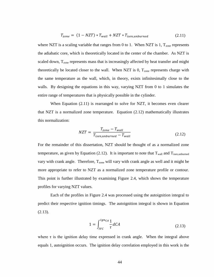
44

(2.11)

where NZT is a scaling variable that ranges from 0 to 1. When NZT is 1, Tzone represents

the adiabatic core, which is theoretically located in the center of the chamber. As NZT is

scaled down, Tzone represents mass that is increasingly affected by heat transfer and might

theoretically be located closer to the wall. When NZT is 0, Tzone represents charge with

the same temperature as the wall, which, in theory, exists infinitesimally close to the

walls. By designing the equations in this way, varying NZT from 0 to 1 simulates the

entire range of temperatures that is physically possible in the cylinder.

When Equation (2.11) is rearranged to solve for NZT, it becomes even clearer

that NZT is a normalized zone temperature. Equation (2.12) mathematically illustrates

this normalization:

(2.12)

For the remainder of this dissertation, NZT should be thought of as a normalized zone

temperature, as given by Equation (2.12). It is important to note that Twall and Tisen,unburned

vary with crank angle. Therefore, Tzone will vary with crank angle as well and it might be

more appropriate to refer to NZT as a normalized zone temperature profile or contour.

This point is further illustrated by examining Figure 2.4, which shows the temperature

profiles for varying NZT values.

Each of the profiles in Figure 2.4 was processed using the autoignition integral to

predict their respective ignition timings. The autoignition integral is shown in Equation

(2.13).

(2.13)

where τ is the ignition delay time expressed in crank angle. When the integral above

equals 1, autoignition occurs. The ignition delay correlation employed in this work is the

45

correlation developed by He et al. at the University of Michigan based on rapid

compression data of mixtures relevant to HCCI combustion [82]:

(2.14)

where τ is the ignition delay time in milliseconds, p is pressure in bar, ϕ is the molar

equivalence ratio, and XO2 is the molar concentration of O2.

The ignition timing predicted by the autoignition integral of each temperature

contour in Figure 2.4 is represented by the yellow stars. Distinct temperature profiles

were chosen and shown in Figure 2.4 ranging from an NZT of 0.76 to 0.96 in increments

of 0.02. However, any value of NZT can be simulated. These values were chosen to

help demonstrate the range of relevant NZT values and their ignition timing. NZT = 0.96

has the highest temperature throughout the compression process. Therefore, it ignites

first and there is no additional compression from combustion elsewhere in the cylinder.

As NZT decreases, the compression temperature is scaled down, the ignition timing is

delayed, the charge is compressed by combustion elsewhere, and eventually ignition

occurs. The compression hump from combustion elsewhere has a significant effect on

the ignition of subsequent zones. First, during the compression hump the ignition timing

of subsequent zones is accelerated. Second, a number of zones achieve ignition that

might not have otherwise. Last, after the peak pressure is reached and the unburned

temperatures begin to fall, the chances of a zone igniting quickly become less likely. An

NZT of 0.78 was the last (coldest) zone to ignite for this data point. The profile for NZT

= 0.76 is shown for completeness but continues throughout the expansion process.

46

Figure 2.4 − Temperature profiles for varying NZT and their respective ignition timings

predicted by the autoignition integral

-120 -60 0 60 120400

500

600

700

800

900

1000

1100

1200


Zo

ne

Te

mp

era

ture

[K

]

NZT= 0.76 : 0.02 : 0.96

NZT= 0.96

NZT= 0.76

a)

-30 -20 -10 0 10 20 30850

900

950

1000

1050

1100

1150


Zo

ne

Te

mp

era

ture

[K

]

NZT= 0.76 : 0.02 : 0.96

NZT= 0.96

b)

NZT= 0.76

47

Later, it will be necessary to switch from normalized to non-normalized forms.

To do this, an arbitrary crank angle must be selected, since a given NZT corresponds to a

temperature profile that varies with crank angle. Once an arbitrary crank angle is chosen,

the isentropic unburned and wall temperatures are used to add or remove the

normalization.

Figure 2.5a is another representation of the data presented in Figure 2.4. Figure

2.5a shows the ignition phasing predicted by the autoignition integral versus varying

normalized zone temperature, NZT. As the normalized temperature decreases, the

ignition phasing is delayed. There is a normalized temperature asymptote, below which

ignition does not occur. The mass below this temperature contributes to the elevated

unburned hydrocarbon emissions and decreased combustion efficiency associated with

HCCI combustion. Note that the relationship depicted in Figure 2.5a is a relationship

between normalized zone temperature and its crank angle of ignition.

Figure 2.5b shows the mass fraction burned curve for this operating condition.

The previous section discussed how the mass fraction burned curve is derived from the

pressure data. Note that the mass fraction burned curve is a relationship between mass

fraction burned and crank angle.

To reiterate, Figure 2.5a is a relationship between normalized temperature and

crank angle and Figure 2.5b is a relationship between mass fraction burned and crank

angle. By setting the crank angle variable equal to each other, it can be eliminated and a

new relationship between mass fraction and normalized temperature can be created. This

new relationship is shown in Figure 2.5c and is termed the NZT-MFB curve. By

equating the ignition phasing predicted by the autoignition integral to the mass fraction

burned curve, the temperature zones, which previously did not have any mass associated

with them, are now related to the mass fraction burned. This NZT-MFB curve depicts

the distribution of mass and temperature that exists in the cylinder prior to ignition for a

specific combustion event.

48

However, the two crank angle variables were not perfectly identical. In the case

of the ignition phasing predicted by the autoignition integral, the crank angle variable is

the crank angle of ignition of each zone. In the case of the mass fraction burned curve,

the crank angle variable is the crank angle of mass burned. By setting these two variables

equal to each other, there is an implicit assumption that once a zone ignites, it burns

instantaneously. Another way of thinking of this assumption is that the chemical reaction

rates associated with energy release are very fast compared to the staggering of ignition

phasing caused by thermal stratification and the global energy release rate is never

limited by the chemical kinetics (Fast Chemistry assumption). A comparison of detailed

chemical kinetic modeling of HCCI with experimental data revealed that the pressure rise

rate of a completely homogeneous cylinder limited only by the chemical reaction rates

was more than an order of magnitude faster than the pressure rise rate that was

experimentally observed for a similarly phased case [83]. Since the chemical kinetics do

not limit the overall combustion event, it is valid to assume that once a zone ignites, it

burns instantaneously, at least during the main part of combustion (10% to 90% of the

mass burned). Chapter 3 is a more thorough validation of the Thermal Stratification

Analysis and the required assumptions.

Another underlying assumption of this analysis is that there is no heat or mass

transfer between zones. In other words, the hot burned gases do not mix with the cold

unburned gases and accelerate their subsequent ignition timing (No Mixing assumption).

This assumption arises from the use of Equation (2.10) to model behavior of the charge

after combustion starts. Equation (2.10) includes the compression work from combustion

elsewhere, which is an effect that needed to be accurately captured. However, there is no

term in Equation (2.10) that could account for a temperature increase due to heat transfer

from the burned gas. The chemiluminescence images taken by Dec et al. [14] visually

show that the time scales, at least during the main combustion event, are too small for

turbulent mixing of burned and unburned gases. However, this was for an operating

49

condition with a very fast burn rate because it lacked internal residuals and was phased

with the crank angle location of the 50% burned point (CA50) at TDC. It is unclear how

valid this No Mixing assumption is as the burn rates are slowed from retarded

combustion phasing and the presence of EGR. The next chapter provides a more in depth

validation effort to determine the conditional validity of the No Mixing assumption.

In the future, a term could be added to Equation (2.10) to account for the heat

transfer and mixing between the burned and unburned regions. At this point, it is not

clear what functional form this mixing term would take and how it would be

implemented in a post-processing setting. The purpose of this work is to propose a

reduced order model or a first approximation of the behavior of the HCCI combustion

process. The analysis can be refined or supplemented in the future as the interactions

between burned and unburned gases in an HCCI engine become better understood. Later,

the analysis in its current form with all of the necessary assumptions will be validated

against CFD simulations and optically measured temperature distributions to determine

the accuracy and applicability of this first approximation of the HCCI energy release

process.

Lastly, assuming that the auto-ignition integral can be used to predict ignition

phasing implies that there are no flames in the combustion chamber that would cause a

zone to ignite prior to the prediction of the autoignition integral (No Flames assumption).

Researchers have imaged HCCI using a borescope, high speed cameras to capture

chemiluminescence, or other techniques and found that this assumption is valid as long as

there is no spark event or hot surface ignition source [11-16]. In addition to these optical

investigations, there has been significant research recently around flame propagation in

highly dilute mixtures, as it pertains to SACI combustion [84-87]. Martz et al. showed

that during the spontaneous ignition event, the mass burned by flame propagation is

“relatively insignificant” due to the very slow flame speeds in highly dilute mixture and

the fast autoignition sequence [84]. Flames may play more of a role over the last 10% of

50

mass to burn because the energy release process is slower, therefore allowing more time

for the flames to propagate. But during the bulk of the heat release (10% to 90%), the

autoignition sequence is too fast and the flames speeds are too slow for a flame to

consume any non-negligible amount of mass.

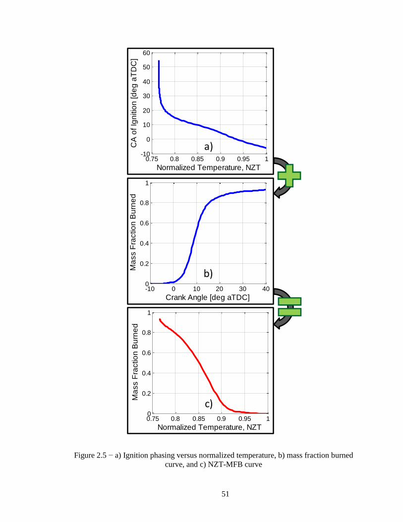
51

Figure 2.5 − a) Ignition phasing versus normalized temperature, b) mass fraction burned

curve, and c) NZT-MFB curve

0.75 0.8 0.85 0.9 0.95 10

0.2

0.4

0.6

0.8

1

Normalized Temperature, NZT

Ma

ss F

ractio

n B

urn

ed

-10 0 10 20 30 400

0.2

0.4

0.6

0.8

1


Ma

ss F

ractio

n B

urn

ed

0.75 0.8 0.85 0.9 0.95 1-10

0

10

20

30

40

50

60


CA

of Ig

nitio

n [d

eg

aT

DC

]

a)

b)

c)

52

Figure 2.5c does in fact depict the distribution of mass and temperature in the

cylinder, but not in a way that is easy to visualize. Therefore, the data in Figure 2.5c can

be rearranged in a more visually intuitive manner. Since the equations characterize the

unburned temperatures in the chamber, the distribution that was determined through the

transformation illustrated in Figure 2.5 is an unburned temperature distribution. Thus, it

is more appropriate to plot the y-axis in Figure 2.5c as the unburned mass fraction rather

than the mass fraction burned. By subtracting the y-data in Figure 2.5c from 1, the

unburned mass fraction is plotted and the distribution that results is the cumulative

distribution function (CDF) shown in Figure 2.6. The cumulative distribution function is

much easier to visually interpret. For example, for this data point, the CDF reveals that

about 90% of the mass is at a normalized temperature of 0.90 or lower, and about 20% of

the mass is at a normalized temperature of 0.80 or lower. Therefore, 70% of the mass is

in the normalized temperature range from 0.80 to 0.90. The CDF can be used in this way

to better understand and study the distributions of mass and temperature that exist in the

cylinder prior to ignition and the operating parameters that affect these distributions.

Note that if the unburned mass fraction was plotted in Figure 2.5b instead of the mass

fraction burned, the transformation to determine the relationship in Figure 2.5c would

directly solve for the mass CDF and the additional step would not be needed.

Probability theory states that the derivative of the CDF is the probability density

function (PDF). The PDF for this data point is also shown in Figure 2.6. The PDF is the

most convenient visualization of the distribution of mass over the range of temperatures

that exist in the cylinder prior to ignition. The PDF states that the probability of finding

mass at near-adiabatic conditions is relatively low. The highest probability of finding

mass in the cylinder occurs at a normalized temperature of about 0.87 for this case. As

the normalized temperature further decreases, the probability of finding mass at that

temperature becomes less and less likely.

53

From Figure 2.6, it would seem that there is really no adiabatic core, or at least,

that only a negligible amount of mass is adiabatic. This would be a very interesting

finding since the consensus in the community is that some percent of the mass is

adiabatic. However, this technique and the way the normalization was arranged through

the equations include the errors in the trapped mass and IVC temperature. The

uncertainty in the trapped mass estimation makes it very difficult to conclude if there is

or is not an adiabatic core and how much mass is adiabatic.

Figure 2.6 − Cumulative distribution function and probability density function

2.2.2 Extension to the Unburned Mass

The analysis thus far only includes the burned mass. The area under the PDF in

Figure 2.6 integrates to a value equal to the combustion efficiency for that operating

condition. Additionally, the coldest mass that burns exhibits some unusual behavior. In

0.75 0.8 0.85 0.9 0.95 10

0.2

0.4

0.6

0.8

1

Ma

ss C

DF


0.75 0.8 0.85 0.9 0.95 10

2

4

6

8

10

Ma

ss P

DF

Mass CDF

Mass PDF

54

Figure 2.6, the coldest edge of the PDF sharply curls upward, because the last mass burns

later, colder, and slower than the rest. In this case, the mass under the “hitch” is about

9% of the total mass. This irregular behavior, which is even more pronounced for the

operating condition with late combustion phasing, is due to the breakdown of the No

Mixing assumption and the Fast Chemistry assumption.

Since the behavior of this small percent of the mass is inconsistent with the main

TSA assumptions, and inconsequential for the overall assessments of thermal

stratification, it is discarded from the CDF and PDF distributions. This discarded mass is

then grouped with the unburned mass and re-included in the overall distribution. To add

the neglected mass onto the distribution, an assumed functional form is needed. Lucht

used coherent anti-Stokes Raman scattering (CARS) to measure the gas temperature near

the wall and found that the gas temperature near the wall follows a logarithmic shape

[89]. Eq. (2.15) below shows Lucht’s correlated temperature profile near the wall:

(2.15)

where Δ and δT are fit constants that vary with crank angle and z is distance from the

wall in [mm]. This particular correlation cannot be used to fit the unburned mass to the

CDF and PDF, since the correlation was developed on a very different engine and

combustion mode (an SI engine with a low compression ratio). However, Lucht’s

correlation indicates that the functional form for the temperature distribution near the

wall is logarithmic, which is in good agreement with “Law of the Wall” from fluid

mechanics. By rearranging the equation above to solve for distance from the wall,

relating distance from the wall to mass, and noticing that within Eq. (2.15), there is a term

that closely resembles NZT in Eq. (2.12), the neglected mass can be modeled with the

following exponential function and new fit constants:

(2.16)

55

where A and B are fit constants that are determined for each data point. The value of the

CDF and the PDF are used to solve for A and B to fit the exponential function in Eq.

(2.16) to the low temperature end of the distribution, thus replacing what was formerly a

“hitch”. Figure 2.7 shows the same PDF from Figure 2.6 with the non-physical mass

discarded and the new exponential fit shown as the dashed blue line. Note the good

agreement between the slope of the exponential fit and the slope of the PDF. The values

of the CDF and PDF are explicitly matched through the selection of the constants (A and

B). However, the slope was not explicitly matched and the good agreement indicates that

the exponential functional form is an appropriate choice, as supported by Lucht’s CARS

measurements and the use of “Law of the Wall” in CFD analysis. In addition, the

location where the exponential fit matches the mass PDF identifies the percent mass

where the main TSA assumptions are no longer valid.

Figure 2.7 − Mass PDF with exponential fit for the unburned and discarded part

0.7 0.75 0.8 0.85 0.9 0.95 10

1

2

3

4

5

6

7

8

9

10


Ma

ss P

DF

Mass PDF

Exponential Fit

Discarded Part

56

Figure 2.8 shows the final, complete normalized temperature distribution from 0

to a little over 1. Remember that a normalized temperature of 0 is the same temperature

as the wall, and a normalized temperature of 1 corresponds to the adiabatic core.

Figure 2.8 – Complete normalized temperature distribution

The entire analysis relies on the measure cylinder pressure and the pressure time

history, in the context of the cylinder volume. From the pressure-volume-crank angle

relationship and the ratio of specific heats of the mixture, the traditional heat release

analysis can calculate the apparent heat release and the mass fraction burned data. Using

the same pressure-volume-crank angle relationship and the ratio of specific heats of the

mixture, the TSA is able to calculate an unburned temperature distribution prior to

ignition. In this way, the resulting unburned temperature distributions are derived from

the pressure trace. If the pressure trace was different, the resulting unburned temperature

0 0.2 0.4 0.6 0.8 10

1

2

3

4

5

6

7

8

9


Ma

ss P

DF

57

distribution would also be different. For example, the mean normalized temperature,

variance, and skewness would all be impacted by changes to the original pressure trace.

2.2.3 Removing the Normalization

The chemical kinetics that drive HCCI combustion are sensitive to absolute

temperatures, rather than normalized temperatures. For this reason, it may be desired to

plot the mass CDF and PDF against absolute temperature to study the effect that different

operating conditions will have on the distribution of mass and temperature and how that

will in turn affect the chemical kinetics. This will be especially important when

examining these CDFs and PDFs over parametric sweeps.

The goal of the analysis is to use the combustion event to determine an unburned

temperature distribution, then to study that unburned temperature distribution over

parametric sweeps, and at different crank angles as if it were a motored cycle rather than

a fired cycle, in the same way that optical researchers are able to study the temperature

distribution over the compression and expansion process in a motored cycle [43, 45]. It

is important to keep this goal in mind while removing the normalization.

To remove the normalization, there are two important details that must be

considered. First, a given NZT corresponds to a temperature profile that varies with

crank angle, as shown in Figure 2.4. That means that the normalized temperature

distribution in Figure 2.6, 2.7, and 2.8 can be plotted at any crank angle desired. It is

unclear at this point how accurate it is to extrapolate the normalized temperature

distribution calculated from the combustion event back to early in the compression stroke

or late in the expansion stroke. Chapter 3 is the validation of the TSA and will shed more

light on the accuracy of this extrapolation. The second important detail is that when

removing the normalization, both the adiabatic unburned temperature and the wall

58

temperature are used, as in Equation (2.11), to convert the normalized temperatures into

absolute temperatures. Instead of using the isentropic unburned temperature as the

adiabatic unburned temperature to remove the normalization, a new temperature is

introduced called the isentropic simulated motoring temperature, shown in Equation

(2.17):

(2.17)

where the simulated motoring pressure is a pressure that matches the measured cylinder

pressure during compression but continues through expansion as a motored cycle would

without the increase from combustion. Equation (2.17) is the same functional form as

Equation (2.10) for the isentropic unburned temperature. The only difference is that the

cylinder pressure in the numerator is replaced with the simulated motoring pressure. In

this way, the isentropic unburned and the isentropic simulated motoring temperature will

be identical before combustion starts. Once some energy is released, the isentropic

unburned temperature will include the compression hump from combustion elsewhere in

the cylinder, while the isentropic simulated motoring temperature does not. Figure 2.9

shows a comparison between the isentropic unburned and isentropic simulated motoring

temperatures. The measured wall temperature is also shown in Figure 2.9 for reference.

59

Figure 2.9 – Isentropic temperature comparisons with the measured wall temperature

To review, the isentropic unburned temperature is used to create the temperature

normalization and predict ignition timing. It is crucially important to use the isentropic

unburned temperature for the ignition timing predictions because without the

compression hump from combustion elsewhere, the ignition timing predictions would be

significantly different. Once the normalized temperature distribution has been

determined, to plot the distribution on an absolute temperature axis, the isentropic

simulated motoring temperature is used, which is a variation of the isentropic unburned

temperature and it allows the unburned temperature distribution to be plotted at any crank

angle as if it were a motored cycle rather than a fired cycle. The interplay between these

equations is a subtlety of the analysis and one of the more difficult details to understand.

Figure 2.10 shows the mass CDF and PDF versus absolute temperature at TDC.

Figure 2.5b is the mass fraction burned curve for this data point and it shows that at TDC,

-120 -60 0 60 120300

400

500

600

700

800

900

1000

1100

1200

1300


Te

mp

era

ture

[K

]

Isen,Unburned

Isen,Sim,Mot

Wall

60

there has been some small amount of energy release. That means that the unburned

temperature distribution plotted in Figure 2.10 does not physically exist at TDC because

the hottest few percent has already burned by TDC and its temperature has greatly

increased. While the distribution as plotted in Figure 2.10 may not physically exist, it is

still useful to plot at a given constant crank angle for comparing to other operating

conditions to understand how operating parameters affect the unburned temperature

distribution prior to ignition. The same technique was used in [90] for studying the

“virtual” conditions at TDC. Later in this dissertation, the unburned temperature

distributions over various engine operating condition sweeps will be plotted at TDC to

study the effect of varying operating conditions on the unburned temperature distribution

at TDC. This is an example of how first the burn characteristics are used to determine the

normalized temperature distribution. Then the distributions are plotted as if it were a

motored cycle, neglecting the heat release.

61

Figure 2.10 – Mass CDF and PDF versus absolute, unburned charge temperature

Figure 2.11 is a three dimensional surface plot of the distribution of the mass and

temperature over the compression and expansion strokes as if it were a motored cycle.

To reiterate, the distribution was calculated based on the burn characteristics, then

extrapolated to any crank angle during the closed part of the cycle. It is unclear how

accurate this extrapolation is, but Chapter 3 will shed light on the accuracy of the

extrapolation. Note that the PDF in Figure 2.10 is a cross section of Figure 2.11 at TDC.

When the normalized temperature distribution is plotted at all of the crank angles during

the closed part of the cycle, as in Figure 2.11, the absolute temperature distribution is

broadest at TDC and narrower early in the compression stroke and late in the expansion

stroke. This phenomenon can be explained by studying Figure 2.8 and 2.9. To create the

three dimensional surface plot in Figure 2.11, the NZT of 0 in Figure 2.8 is aligned with

880 940 1000 1060 11200

0.2

0.4

0.6

0.8

1

Ma

ss C

DF

Unburned Temperature at TDC [K]

880 940 1000 1060 11200

0.003

0.006

0.009

0.012

0.015

Ma

ss P

DF

Mass CDF

Mass PDF

62

the red wall temperature line Figure 2.9, while the NZT of 1 in Figure 2.8 aligns with the

blue isentropic simulated motoring temperature in Figure 2.9. With this in mind, the

reason for the broadening of the distribution around TDC is simply because the

temperature difference between the wall and isentropic core is the largest at TDC. Early

in the compression stroke or late in the expansion stroke, the width of the distribution is

much smaller because the difference between the wall temperature and isentropic

simulated motoring temperature is much smaller.

Figure 2.11 – Three dimensional surface plot of the unburned temperature distribution

over the compression and expansion processes

63

Note that the Mass CDF axis has no units in Figure 2.10. Neither does the Mass

PDF axis in Figure 2.10 or 2.11. Technically speaking, to be mathematically consistent,

the units of the Mass PDF axis should be the reciprocal of the x-axis. Therefore, in this

case, the Mass PDF axis should have units of 1/K. In the literature, researchers tend not

to write the units because they are not intuitive and can make it more difficult to

understand the concept of the probability density function. This paragraph recognizes

that to be mathematically accurate, the units of the Mass PDF axis should be 1/K when

plotted against absolute temperatures. But to be consistent with the community and to

avoid confusion, no units will be plotted on any of the Mass PDF plots throughout this

dissertation.

2.2.4 Thermal Width

The mass PDFs and CDFs are an incredibly valuable tool in understanding HCCI

combustion, as optical and CFD researchers have already demonstrated. They are

simultaneously qualitative and quantitative. One way that they will be used to

quantitatively assess the thermal stratification of a particular engine or operating

condition is through the thermal width (TW), which is a metric that is also used by other

HCCI researchers [43, 45]. The thermal width is simply the temperature distance

between two defined points on the mass CDF. The most commonly used values are the

10% to 90% thermal width and the 25% to 75% thermal width. For example, the 10%

point on the CDF in Figure 2.10 is around 945K and the 90% point is around 1047K.

Therefore, the 10% to 90% thermal width for this data point is about 102K. The 25% to

75% thermal width is a good metric for the thermal stratification within the bulk of the

charge, whereas the 10% to 90% thermal width includes some of the tails and the mass

near the wall.

64

2.2.5 Review of the TSA Assumptions

A number of assumptions were made throughout the analysis. This section

reviews the main assumptions required for the TSA to determine an unburned

temperature distribution from a pressure curve. As the assumptions are reconsidered,

keep in mind the new conceptual description of HCCI as a sequential autoignition of

progressively cooler regions with the cooler, later phased regions being compressed by

the energy release from the hotter, earlier phased regions.

The cylinder is assumed to be compositionally homogeneous by the time

combustion begins (Compositionally Homogeneous assumption). The temperature,

however, varies throughout the cylinder and follows the thermodynamic equations

outlined above. The implication of this assumption is that there is no heat or mass

transfer between zones in the cylinder after combustion starts. That is to say that there is

no mixing or heat transfer from the burned zone to the unburned zone (No Mixing

assumption). The next major assumption is that the chemical reactions associated with

heat release are fast compared to the staggering of ignition timing due to thermal

stratification (Fast Chemistry assumption). The autoignition integral and He’s ignition

delay correlation are used to predict ignition, thereby assuming that this correlation can

accurately capture the autoignition behavior and that all of the mass burns by

autoignition. It is assumed that there are no flames in the combustion chamber that

would cause a region to burn earlier than the ignition predictions by the autoignition

integral (No Flames assumption). Lastly, the coldest mass, possibly very close to the

wall, follows an exponential shape described by Equation (2.16) (Exponential Fit

assumption).

These assumptions were necessary for the TSA to calculate an unburned

temperature distribution in an HCCI engine. However, the errors introduced by these

65

assumptions and the conditional validity of the assumptions needs to be assessed.

Chapter 3 discusses two independent efforts to validate the TSA.

2.3 Sensitivity of the TSA to the Ignition Delay Correlation

Section 2.2 described a novel technique developed as part of this thesis that can

calculate an unburned temperature distribution from a pressure trace and heat release.

The analysis relies heavily on ignition timing predictions by the autoignition integral and

He’s ignition delay correlation. This section tests the sensitivity of the TSA results to the

values used in the ignition delay correlation.

2.3.1 Effect of Activation Energy

The exact, correlated and published [82], form of He’s ignition delay correlation,

shown in Equation (2.14), was used in the TSA technique for post-processing the

experimental data collected in Part II of this dissertation. That is to say that neither the

constant in front of the correlation nor the activation energy was changed from the

published values. He’s ignition delay correlation was used because it was developed for

mixtures relevant to HCCI combustion. However, it was correlated to data collected in a

rapid compression facility using isooctane as the fuel. Chapter 4 describes the fuel that

was used to collect the experimental data in Part II of this dissertation, which was a

research grade 87 octane, unoxygenated gasoline. The difference in fuel chemistry

between the fuel that was used to develop the correlation (isooctane) and the fuel used in

this study (gasoline) might suggest that the activation energy in the correlation should be

changed to a value for gasoline. Babajimopoulos compared shock tube data of gasoline

taken by Gauthier et al. [91] to shock tube data for isooctane taken by Davidson et al.

[92] and found that for the high temperature range, the activation energy between the two

66

fuels is not significantly different [90]. Later, surrounding the discussion of Figure 2.17,

it will be shown that the higher temperature range is the only relevant portion of the

ignition delay curve in this practical engine. This gives confidence in the choice of the

He correlation despite the differences in the fuel since it was developed for HCCI-like

mixture compositions. Although there is good confidence in the He correlation and its

applicability to this research, this section tests the sensitivity of the TSA results (namely

the mass PDFs) to changes in the activation energy in the ignition delay correlation

because any correlation has some errors associated with its use.

Figure 2.12 shows the mass PDF results from processing the baseline data point

with the default activation energy as given by He (33,700 cal/mol) represented in the

figure by the red line labeled “Ea/1”, and the activation energy divided by 1.05 and 0.95.

Changing the constant in this way varies the activation energy approximately 5% up and

down from the default value. It can be seen from Figure 2.12 that varying the activation

energy for a given combustion event greatly changes the range of temperatures that the

mass PDF spans with the lowest activation energy spanning the lowest range of

temperatures. The 5% changes to the activation energy cause the temperature range to

vary by 5%. The reason for this relationship is that the activation energy in the ignition

delay correlation in Equation (2.14) is divided by temperature. Therefore, a constant

applied to the activation energy needs to be compensated for with an equal change in the

temperature to give the same ignition characteristics. Besides the shift in the absolute

temperature range, the shapes of the distributions are fairly similar and insensitive to

changes in the activation energy. There is a slight change in height and width of the

distribution with the width of the distribution scaling with the absolute temperature range.

67

Figure 2.12 − Effect of varying the activation energy in the ignition delay correlation on

the mass PDFs

This section discusses the sensitivity of the TSA to the activation energy in the

ignition delay correlation. It is especially important to understand the sensitivity to the

activation energy since the default value is for isooctane and the fuel used in the research

is gasoline. Previous shock tube experiments showed that the value for isooctane and the

value for gasoline is not significantly different [90-92], but it is still important to study

the sensitivity of the results to activation energy. The sensitivity analysis shows that the

absolute temperature range is very sensitive to the activation energy. The shape is also

somewhat sensitive to the activation energy. Using a different value for the activation

energy than the true value may introduce some error. For all of the data collected and

processed in this dissertation, the same fuel was used and the same activation energy was

used. Therefore, if the true activation energy is different from the value used in the

800 900 1000 1100 1200-2

0

2

4

6

8

10

12

14x 10

-3

Temperature at TDC [K]

Ma

ss P

DF

Ea/0.95

Ea/1.0

Ea/1.05

68

correlation, it will impart a constant offset or error to all of the data and all of the trends

presented in this dissertation will still hold valid.

2.3.2 Effect of the Pre-exponential Constant in the Ignition Delay Correlation

In addition to the activation energy, the sensitivity of the mass PDFs to the pre-

exponential constant is studied in this section. Figure 2.13 shows the results from the

pre-exponential sensitivity study. Each curve in Figure 2.13 corresponds to multiplying

the ignition delay correlation (IDC) by a factor of 2. The results in Figure 2.13 are very

similar to those in Figure 2.12 except that the mass PDFs are much more sensitive to

changes in the activation energy, since Figure 2.12 corresponded to around 5% changes

whereas Figure 2.13 corresponds to factors of 2. Again, if the ignition delay time is

scaled up or down by a factor of 2, the temperature increases or decreases so that ignition

occurs at the crank angles prescribed by the mass fraction burned curve. As the

maximum adiabatic temperature increases or decreases with the pre-exponential constant,

the height and width of the distribution are again affected in the same way as the

variation of activation energy.

Just as with the activation energy study, any error introduced by using a value for

the pre-exponential constant that is different from the true value for this fuel will only

affect the absolute position of the distribution on the temperature axis. The trends will

hold true when comparing one operating condition to one another because the same fuel

was used and the same ignition delay correlation was used for all of the data collected

and processed.

69

Figure 2.13 − Effect of varying the pre-exponential constant in the ignition delay

correlation on the mass PDFs

2.3.3 Effect of the Negative Temperature Coefficient Region in the Ignition Delay

Correlation

He’s ignition delay correlation appears as a straight line with constant slope when

the ignition delay time is plotted on a logarithmic vertical axis against 1000 divided by

the temperature on the horizontal axis. Realistically, researchers have observed a

negative temperature coefficient (NTC) region of the ignition delay curve depending on

the fuel and the conditions. In an attempt to capture the NTC region and the behavior of

isooctane, Goldsborough introduced an ignition delay correlation that includes the NTC

region based on the conditions [93]. Please refer to [93] for more information on

Goldsborough’s ignition delay correlation. A plot of ignition delay predictions by both

He’s ignition delay correlation and Goldsborough’s ignition delay correlation is shown in

800 850 900 950 1000 1050 1100 1150-2

0

2

4

6

8

10

12

14x 10

-3


Ma

ss P

DF

0.5*IDC

1.0*IDC

2*IDC

70

Figure 2.14 with the ignition delay times predicted by He’s ignition delay correlation

shown as the dashed blue line and the predictions by the Goldsborough correlation are

shown in the solid red line. These ignition delay times were calculated for the baseline

operating condition over the compression process. In that way, the results in Figure 2.14

do not correspond to any one pressure condition. Instead, these ignition delay predictions

correspond to the isentropic unburned temperature and the measured cylinder pressure

over the compression process. That is why there is an ever so slight curve to the dashed

blue line, rather than it being perfectly straight. Note the strong similarities between the

two correlations for the high temperature range. At temperatures below 833 K, the

Goldsborough correlation has a negative temperature coefficient region where the

ignition delay times are greatly reduced in comparison to the He ignition delay

correlation.

Figure 2.14 – Comparison of the He and Goldsborough ignition delay correlations

0.8 1 1.2 1.4 1.6 1.8 210

-6

10-4

10-2

100

102

104

106

1000/T [1/K]

Ign

itio

n D

ela

y [s]

Goldsborough NTC Correlation

He Correlation

71

The previous two sections experimented with the sensitivity of the TSA results to

the constants in the ignition delay curve. The purpose of this section is to observe the

effect of the NTC region on the TSA results. Although the ignition delay correlations are

very similar in the high temperature range, the slight differences are enough to give

different resulting unburned temperature distributions. Since the goal is to only observe

the effect of the NTC region, a hybrid ignition delay correlation was created and it is

shown in Figure 2.15. This hybrid ignition delay correlation exactly equals the He

ignition delay correlation at temperatures above 836 K and the hybrid correlation exactly

equals the Goldsborough ignition delay correlation at temperatures below 836 K. Note

that 836 K is the point below which the two correlations deviate. By comparing the

results from processing the same operating conditions with the He correlation and with

the hybrid correlation, the effects of the NTC region alone on the TSA results can be

determined.

72

Figure 2.15 – Comparison of the He and the Goldsborough ignition delay correlation

showing the hybrid correlation for determining the effects of the NTC region on the TSA

results

First, the He correlation and the hybrid correlation are used to process the baseline

operating condition to determine the effects of the NTC region around the baseline

conditions. Figure 2.16 shows the unburned temperature distributions at TDC calculated

once using the He ignition delay correlation and once using the hybrid He correlation

with the NTC region shown in Figure 2.15. The unburned temperature distributions in

Figure 2.16 are identical for all intents and purposes. There are no perceivable

differences between the distributions calculated with and without the NTC region. These

results show that for the baseline conditions the lack of the NTC region in the He

correlation is not imparting any errors onto the results.

0.8 1 1.2 1.4 1.6 1.8 210

-6

10-4

10-2

100

102

104

106

1000/T [1/K]

Ign

itio

n D

ela

y [s]

Goldsborough

He

Hybrid Correlation

73

Figure 2.16 – Unburned temperature distributions calculated with the He correlation and

the hybrid He NTC correlation

The reason that the lack of the NTC region does not affect the ignition timing

predictions is that the significant contributions to the autoignition integral occur at

temperatures that are above the NTC region. Figure 2.17 illustrates this point by showing

the autoignition integral and 1000/T. When the autoignition integral crosses 1,

autoignition occurs. There are no significant contributions to the autoignition integral

before 40 crank angle degrees bTDC. In fact, all the significant contributions to the

autoignition integral occur after about 35 crank angle degrees bTDC. The values of

1000/T that are in the same range of crank angle degrees are less than 1.2. That means

that if the temperature is below 833 K, the contributions to the autoignition integral are

insignificant, whereas if the temperature is above 833 K (1.2 in terms of 1000/T), the

contributions to the autoignition become significant. Temperatures greater than 833 K in

800 850 900 950 1000 1050 11000

0.002

0.004

0.006

0.008

0.01

0.012

0.014


Ma

ss P

DF

He Correlation

Hybrid He NTC Correlation

74

Figure 2.17 are above the NTC region and the correlations collapse. This is why there is

no difference between the distributions in Figure 2.16.

Figure 2.17 – Contributions to the autoignition integral and 1000 over the isentropic

unburned temperature

In addition to the baseline conditions, a low engine speed (800 rpm) operating

condition was studied to examine the effect of the NTC region on the TSA results for a

worst case scenario. At lower speeds the ignition delay times are generally longer,

pushing operation closer to the NTC region on the ignition delay curve. 800 rpm is 400

rpm lower than any other data point collected and 1200 rpm lower than the baseline

operating condition. Figure 2.18 shows the calculated mass PDFs from using the He

correlation and the hybrid He NTC correlation. The difference between the two PDFs is

very small even for this low speed point giving good confidence that the NTC region is

not significantly affecting the TSA results. In fact, the linear shift is less than 1 K. The

correlation with the NTC region is at lower temperatures (only by less than 1 K) than the

-120 -100 -80 -60 -40 -20 0 200

0.2

0.4

0.6

0.8

1

1.2

1.4

1.6

1.8


1000/T [1/K]

Autoignition Integral

75

He correlation without the NTC region because the NTC region contributes some small

amount to the autoignition integral, allowing the temperatures to be lower and still give

the same ignition timing.

Figure 2.18 − Effect of the NTC region on the mass PDFs for a low speed (800 rpm)

point

2.4 Chapter Summary

This chapter proposed a novel post-processing methodology for studying thermal

stratification in a fired metal HCCI engine. The technique uses the autoignition integral,

with the assumption that the mass in the cylinder follows a self-similar temperature

contour, to predict ignition phasing of different temperature profiles. The unburned

charge temperature profiles are calculated based on the thermodynamic relations for

isentropic compression. Then, by comparing the ignition phasing of the different

temperature profiles to the mass fraction burned data and assuming that the staggering of

800 850 900 950 1000 10500

0.002

0.004

0.006

0.008

0.01

0.012

0.014


Ma

ss P

DF

He Correlation

Hybrid He NTC Correlation

76

ignition phasing due to temperature stratification is the rate limiting factor in the global

combustion event, rather than the chemical reaction rates, a distribution of mass and

temperature in the cylinder prior to combustion can be determined. The behavior near

the wall was non-physical because the TSA assumptions are no longer valid for the

coldest mass to burn. Therefore, the non-physical behavior was discarded from the

distribution and the mass near the wall was included on the end of the distribution by an

exponential fit, which is in good agreement with the CARS measurements by Lucht and

the “Law of the Wall” from fluid mechanics. With the unburned mass fit with an

exponential function to the cold side of the distribution, all of the mass in the cylinder is

included in the distribution and the distributions are ready to be validated and studied.

These temperature distributions can be compared over various engine operating

conditions to study and better understand the development and effect of naturally-

occurring thermal stratification.

Lastly, the sensitivity of the distributions to the ignition delay correlation and its

constants was studied to understand how differences in the fuel chemistry may impact the

distributions.

77

CHAPTER 3

VALIDATION OF THE THERMAL STRATIFICATION ANALYSIS

The preceding chapter described a methodology for creating a cylinder-wide

temperature distribution from a pressure trace. The distributions seem to be in good

agreement with intuition. However, several assumptions were made, and the magnitude

of the errors introduced by these assumptions needs to be characterized before the

analysis can be considered to be valid.

The following sections describe two ways in which the TSA has been validated.

First, the TSA is used to process output data from CFD simulations and the results are

compared to the known CFD temperature distributions. Second, the TSA-determined

temperature distributions are compared to optically measured distributions in a research

engine at Sandia National Laboratories.

3.1 Validation against Computational Fluid Dynamics Simulations

To determine the validity of the TSA, CFD output data is processed with the TSA

as if it were experimental data, and the analysis-derived temperature distributions are

compared to the known CFD distributions. This method mostly helps to assess the

soundness of the Fast Chemistry assumption, because the CFD uses a 197 species skeletal

kinetics mechanism [61] based on the Lawrence Livermore National Laboratory detailed

isooctane mechanism with 857 species [62], whereas the TSA assumes fast energy

release chemistry. The use of the autoignition integral, the ignition delay correlation, and

the Fast Chemistry assumption may produce an unrealistic hottest edge of the

78

distribution. Figure 3.1 shows the burn characteristics of a single zone HCCI combustion

model at similar conditions to the experimental data collected as part of this dissertation.

The mass fraction burned curve in Figure 3.1 shows that the Fast Chemistry assumption

is most valid for the 20% burned point to the 99% burned point. In fact, the duration

from 20% burned to 99% burned is only 0.8 crank angle degrees. This gives confidence

in the fast chemistry assumption for the majority of the charge. However, the first 20%

of the mass burns more slowly over a longer duration. This energy release is due to pre-

ignition kinetics, i.e. the small fraction of energy release before the main autoignition

event. These pre-ignition kinetics pose a problem for the TSA because the TSA will

interpret this energy release as mass at a higher temperature due to the Fast Chemistry

assumption and may potentially result in errors on the leading edge of the distribution.

The following sections will help to validate the magnitude of the errors introduced by this

assumption, and the other TSA assumptions.

79

Figure 3.1 – Mass fraction burned curve for a single zone HCCI combustion model at

conditions representative of the experimental data

Several previously run CFD simulations [61] were processed with the TSA as if

the CFD results were experimentally collected data. The CFD-predicted pressure and the

conditions at IVC were used in the analysis. The resulting TSA-based temperature

distributions are then compared to the known CFD temperature distributions over an IVC

temperature sweep. An IVC temperature sweep was used to assess the robustness of the

Fast Chemistry assumption when combustion phasing is retarded and burn rates decrease.

Figure 3.2 show three separate CFD runs that were used to validate the TSA. The

CA50 phasings of the data points in Figure 3.2 are approximately 5 CA after top dead

center (aTDC), 12.5 CA aTDC, and 20.5 CA aTDC, respectively. These three

simulations were processed with the TSA and the results were compared to the known

CFD distributions.

-20 -10 0 10 200

0.1

0.2

0.3

0.4

0.5

0.6

0.7

0.8

0.9

1


Ma

ss F

ractio

n B

urn

ed

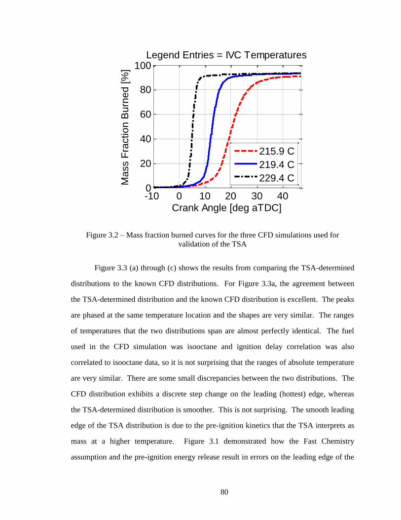
80

Figure 3.2 – Mass fraction burned curves for the three CFD simulations used for

validation of the TSA

Figure 3.3 (a) through (c) shows the results from comparing the TSA-determined

distributions to the known CFD distributions. For Figure 3.3a, the agreement between

the TSA-determined distribution and the known CFD distribution is excellent. The peaks

are phased at the same temperature location and the shapes are very similar. The ranges

of temperatures that the two distributions span are almost perfectly identical. The fuel

used in the CFD simulation was isooctane and ignition delay correlation was also

correlated to isooctane data, so it is not surprising that the ranges of absolute temperature

are very similar. There are some small discrepancies between the two distributions. The

CFD distribution exhibits a discrete step change on the leading (hottest) edge, whereas

the TSA-determined distribution is smoother. This is not surprising. The smooth leading

edge of the TSA distribution is due to the pre-ignition kinetics that the TSA interprets as

mass at a higher temperature. Figure 3.1 demonstrated how the Fast Chemistry

assumption and the pre-ignition energy release result in errors on the leading edge of the

-10 0 10 20 30 400

20

40

60

80

100


Ma

ss F

ractio

n B

urn

ed

[%

]

Legend Entries = IVC Temperatures

215.9 C

219.4 C

229.4 C

81

distribution. The peak of the TSA-determined PDF is slightly lower than the known CFD

distribution, again due to the smoothing of the distribution and the “extra” mass on the

leading edge of the TSA PDF. On the colder side, the CFD distribution has bumps that

correspond to the mass in the crevices and the ring pack volumes. The TSA uses an

exponential fit for this mass, since that mass is too cold to burn and the TSA does not

have any ignition timing information for it. While the exponential fit cannot capture the

bumps from the crevice volumes, it does a good job capturing the overall trend near the

wall.

Figure 3.3b again shows the comparison between the known CFD PDF and the

TSA-determined PDF now for a mid-phased run with CA50 around 12.5 CA aTDC. The

agreement is also very good and the explanation is similar to that of Figure 3.3a. Figure

3.3c shows the comparison for a very late phased, slow burning, CFD run, with CA50

phasing 20.5 CA aTDC. The agreement between the TSA-determined distribution and

the known CFD distribution has deteriorated. The over prediction by the TSA now starts

with the leading edge and continues through the bulk of the charge. The exponential fit

now poorly captures the trend of the distribution near the wall because of the over

prediction throughout the rest of the distribution. The reason for the over prediction of

mass is likely due to the breakdown of the No Mixing assumption and the Fast Chemistry

assumption. The assumptions break down for this late combustion phasing, because the

burn rate slows substantially, thus allowing more time for mixing and increasing the

impact of expansion on charge temperature and energy release reaction rates. If the

burned gas has time to mix with the unburned gas and exchange heat, the unburned gas

will ignite sooner than the prediction by the autoignition integral using Equations (2.10)

and (2.11) for temperature because Equation (2.10) only includes the compression effects

from the piston and from combustion elsewhere, but no heat transfer effects. This will

cause the TSA to over predict the amount of mass at a given normalized temperature and

seem to shift the mass from near the wall to the core.

82

Figure 3.3 − Comparison between the known CFD distribution and the TSA-determined

distribution for (a) an early phased case, (b) a mid-phased case, and (c) a retarded case

with CA50 phasings at 5, 12.5, and 20.5 CA aTDC, respectively

800 850 900 950 10000

0.01

0.02

0.03

0.04

0.05

Temperature at 20 CA bTDC [K]

Mass P

DF

Discarded Part

TSA PDF

CFD PDF

800 850 900 950 10000

0.01

0.02

0.03

0.04

0.05

0.06


Mass P

DF

Discarded Part

TSA PDF

CFD PDF

800 850 900 950 10000

0.01

0.02

0.03

0.04

0.05

0.06


Ma

ss P

DF

Discarded Part

TSA PDF

CFD PDF

(a)

(b)

(c)

83

3.2 Validation against Optically Measured Data

In addition to the CFD validation effort, the TSA-determined distributions have

been validated against optically measured temperature distributions to determine the

validity and accuracy of the analysis against experimental data, rather than a CFD model.

To make this comparison, optical data that was collected from a motored cycle was

processed to create a cylinder-wide distribution. That distribution was then compared to

a TSA-determined distribution created by processing a fired cycle on the same engine.

First, the creation of the optically measured PDF is described: followed by the TSA-

determined PDF.

An optically accessible HCCI engine at Sandia National Laboratories (SNL) was

used to collect the motored and fired data presented below [43, 45]. The engine is a

Cummins B-series six cylinder engine with cylinders 1 through 5 deactivated. The

engine has a displacement of 0.98 liters/cylinder and a compression ratio of 14:1. There

is a piston-crown window, as well as three large windows in the top of the cylinder wall.

For the data presented below, the piston-crown window was not used. Instead, a

vertically oriented laser sheet was directed through one cylinder wall window, while the

camera was aimed through the cylinder wall window that is perpendicular to the laser

sheet. The temperature imaging technique is single-line toluene planar laser induced

fluorescence (PLIF). 96% isooctane and 4% toluene (by volume) were blended upstream

in the intake in a fuel vaporizer. For the motored points, 100% nitrogen was used in

place of air. The engine was run at 1200 rpm, an intake pressure of 100 kPa, an intake

temperature of 170 °C, and a coolant and oil temperature of 100 °C unless otherwise

noted. The optical data used for validation in this study was originally presented in [45].

Please refer to [45] for more details on the data and the collection technique, or refer to

[14, 43-45] for more information on the experimental set-up.

84

The single-shot image is processed as described in [45] to minimize error (caused

by shot-to-shot laser energy variation, distortion, vignetting, etc.) and to determine the

temperature map on the plane of the laser sheet. To accurately compare the optically

measured distribution to the distribution predicted by the TSA, the optically measured

distribution needs to be on a cylinder-wide basis, rather than for the plane of the laser

sheet. Therefore, each pixel from the single cycle image is weighted by its associated

volume around the cylindrical axis. Figure 3.4 is an example illustration. The colder gas

near the cylinder wall will constitute a larger fraction of the three dimensional volume

than the two dimensional area. Therefore, the volume-weighted temperature distribution

will be wider than what is shown in the two-dimensional image. From comparing the

raw measured PDFs and the volume weight PDFs, this effect was noticeable. The peak

of the distribution was slightly lower for the volume weighted PDFs than for the raw

PDFs and the volume weight PDFs were broader than the raw PDFs. But the differences

between the two distributions were relatively small [94].

This method of creating a three dimensional distribution from a two dimensional

image assumes that the thermal stratification displayed in the image is representative of

the temperature distribution throughout the cylinder. However, the volume weighting

was done for 100 individual cycles to reduce the error in assuming the random charge

motion is representative of the whole cylinder. The 100 individual-cycle, volume

weighted distributions were then averaged. Comparing the amount of variation between

the 100 individual-cycle, volume-weighted PDFs gives a general impression of the

amount of error introduced by assuming that the stratification in the 2D image is

representative of the entire cylinder. The difference between the individual-cycle

distributions was small giving good confidence that the 2D image can accurately capture

the thermal stratification throughout the cylinder especially when the individual cycles

are then averaged to give the ensemble averaged temperature distribution [94].

85

Figure 3.4 − Illustration of the image volume weighting to create a cylinder-wide

distribution from a single plane temperature map [94]

The volume weighted (three-dimensional) distribution that results from

processing the optically determined temperature map will be compared to TSA-

determined distributions created by post-processing fired engine data from the same

engine. Fired engine data was collected on the optical engine described above for the

purpose of post-processing with the TSA under two different operating conditions. First,

fired engine data was collected under similar operating conditions to the conditions used

to collect the motored optical data (170 °C intake temperature, 100 °C coolant and oil

temperatures, 1200 rpm). Second, the coolant temperature was decreased by 40 °C to 60

°C and data was collected. The objective of the lower coolant temperature data point was

to better mimic the wall temperature of the motored engine. Under fired conditions, the

wall temperature increases substantially from the heat release from combustion. It was

found that decreasing the coolant temperature 40 °C approximately matched the wall

temperature of the fired experiment to the baseline conditions of the motored experiment.

To match CA50 phasing, the intake temperature needed to increase 16.2 °C with the

lower coolant temperature. The fired data was then processed with the TSA and the

resulting distributions are compared to the optically measured distributions below. The

86

60 °C coolant temperature data point is presented in Figures 3.5 and 3.6. The baseline,

100 °C coolant temperature was used to create the distributions in Figure 3.7 [94].

First, the comparison between the optically measured distributions and the TSA-

determined distributions are presented for -40 CA (40 CA bTDC), -20 CA, TDC, and 20

CA aTDC in Figure 3.5. The ranges of absolute temperatures that the optically measured

PDFs span were not perfectly identical to the ranges for the TSA-determined PDFs

because the conditions were not perfectly identical for the fired and motored data.

Specifically, the motored cycle used 100% nitrogen to ensure no oxidation whereas the

fired data point used air. Therefore, the optical distributions were shifted to align with

the TSA-determined distributions and only the shape of the distribution is used for

validation. As TDC is approached, both the optically measured and the TSA-determined

distributions broaden. The TSA-determined distributions broaden because the adiabatic

temperature is increasing much faster than the wall temperature, as discussed in Chapter

2 around Figure 2.11. The optically measured distributions broaden near TDC because

the adiabatic temperature is increasing much faster than the wall temperature and because

turbulent charge motion is mixing cold near-wall boundary layer gases with the hot core

gases. That is to say that the optically measured distributions capture the development of

the temperature distribution over the compression process. The TSA cannot capture the

development of the temperature distribution. Instead, the TSA takes the calculated

temperature distribution, which is representative of the particular combustion event, and

extrapolates it backward into the compression process. Figure 3.5 shows that this

extrapolation is not very accurate because the temperature distribution develops and

changes over the compression process. Therefore, the TSA results are only valid around

TDC and around the phasing of the combustion event. After TDC, the TSA-determined

distribution narrows because the adiabatic (isentropic simulated motoring) temperature

decreases faster than the wall temperature. The optically measured distributions stay

approximately the same width after TDC. It was proposed that after the peak pressure is

87

reached, a growing boundary layer and out-gassing from crevices prevents the optically

measured distribution from narrowing after TDC [45].

The agreement between the optically measured PDFs and the TSA-determined

PDFs is best at TDC and poor at earlier or later crank angles. At -40 CA and -20 CA, the

optically measured distributions are much tighter than the TSA-determined distributions.

After TDC, the TSA distribution is tighter than the optically measured distribution. It is

not surprising that the best agreement occurs at TDC since CA10, CA50, and CA90 for

this operating condition occur at 4.5 CA, 6.7 CA, and 9.5 CA, respectively. At TDC, the

optical distribution is still slightly tighter than the TSA distribution. This is somewhat

expected as well since about 7.1% of the volume at TDC is in the large top-land crevices

of this optical engine. That is to say that at least 7.1% of the cylinder volume at TDC is

not included in the image and therefore not included in the optically measured

distribution. This mass is relatively cold and would tend to spread the distribution if it

were included.

Note that the comparison was made at additional crank angles but was not plotted

for conciseness. The trend with the additional crank angles was the same as the trend

seen in Figure 3.5 except to a much greater extent. For timings earlier than 40 CA before

TDC, the optically measured distributions were much narrower than the TSA-determined

distributions. After 20 CA after TDC, the TSA-determined distribution continues to

tighten as the optically measured distribution stays roughly the same width. By far the

best agreement between the TSA-determined distribution and the optically measured

distribution occurred around TDC and just after. The agreement is very poor early and

late in the cycle. This proves that the TSA results are most accurate around the phasing

of the combustion event because it relies on the mass fraction burned curve and are not

accurate when the normalize distribution is extrapolated to early in the compression

stroke or late in the expansion stroke, because the real temperature distribution evolves

over the compression and expansion processes and the TSA determines one normalized

88

distribution that is characteristic of the combustion event which occurs around TDC. The

development and evolution of the temperature distribution over the engine cycle can be

seen in Dec’s optical data [43] and in work done by Sjöberg et al. [95].

Figure 3.5 − Comparison between the optically measured distributions and the TSA-

determined distributions at -40 CA, -20 CA, TDC, and 20 CA

Figure 3.6 shows a closer look at the comparison for the most relevant crank

angles for which the comparison can be made (optical data only exists every 10 crank

angle degrees): TDC and 10 CA aTDC. The agreement at TDC is decent. The percent

error at a given temperature is defined as the absolute value of the difference between the

optically measured PDF and the TSA-determined PDF as a percent of the peak of the

optically measured PDF as shown in Equation (3.1) below:

(3.1)

700 750 800 850 900 9500

0.02

0.04

0.06

0.08

0.1

Temperature [K]

Ma

ss P

DF

Optically Measured PDFs = Solid Line TSA-Determined PDFs = Dashed Line

TDC

-40 CA

20 CA

-20 CA

89

The error at TDC is 3.7% on average over the range of temperatures, with a

maximum of 21.6% occurring at 956 K. The mass in the crevice volume, not included in

the image, is a possible explanation for why there is a discrepancy between the two

distributions. At 10 CA aTDC, however, the agreement is excellent. The average error is

only 2.1% with a maximum of 5.8% occurring at 879 K.


determined distributions for the 60 °C coolant temperature data point at TDC and 10 CA

Figure 3.7 shows the comparison between the optically measured distributions at

TDC and 10 CA aTDC and the distributions created from processing the 100 °C coolant

temperature data point. The higher wall temperatures and lower intake temperature cause

a slightly narrower TSA-determined distribution in Figure 3.7 compared to Figure 3.6.

Therefore, the agreement between the optically measured PDFs and the TSA-determined

PDF is better at TDC with an average error of 2.7% and a maximum error of 11.9%

occurring at 962 K. However, the TSA-determined distribution at 10 CA aTDC is now

800 850 900 950 10000

0.01

0.02

0.03

0.04

Temperature [K]

Ma

ss P

DF


TDC10 CA

90

narrower than the optically measured distribution. The average error at 10 CA aTDC is

1.76% with a maximum error of 8.1% occurring at 913 K.


determined distributions for the 100 °C coolant temperature data point at TDC and 10 CA

The good agreement between the known CFD distributions and the TSA-

determined distributions for the early and mid-phased runs, shown in Figure 3.3, and the

good agreement between the optically measured PDFs and the TSA-determined PDFs at

TDC and 10 CA aTDC in Figure 3.6 and Figure 3.7 (i.e. the similarly shaped

distributions and relatively low amounts of error over the entire range of temperature)

provide validation of the TSA methodology and the necessary assumptions.

An important feature of the optically measured comparisons is that the leading

hottest edge of the distribution is always in great agreement in Figure 3.6 and Figure 3.7.

Although, the CFD simulation validation showed errors on the leading edge from the pre-

ignition kinetics, the optically measured data comparison shows great agreement on the

800 850 900 950 10000

0.01

0.02

0.03

0.04

Temperature [K]

Ma

ss P

DF


TDC10 CA

91

leading edge. There are three possible reasons why the error exists for the CFD

simulations but not for the optically measured comparisons. First, in the CFD simulation,

the CFD distribution has a very steep step change leading edge. In which case, all of the

pre-ignition kinetics will coincide and produce a lot of error. The optically measured

distribution does not show a step change on the leading edge and therefore the pre-

ignition kinetics do not coincide, resulting in a smaller, more spread out error. A second

possible explanation as to why the leading edge shows error for the CFD validation but

not for the optically measured validation is that the mechanisms used in the CFD

simulations and in the single zone HCCI model in Figure 3.1 might be over predicting the

amount of energy released by pre-ignition kinetics. In Figure 3.1, the single zone model

predicts around 5-10% of the energy from pre-ignition kinetics. Also, Figure 3.2 shows a

long slow ramp up corresponding to around 5-10% of the mass, particularly noticeable

for the mid and late phased simulations. This long slow ramp up is simply not seen in

experimental data and is an indication that the mechanism may be over predicting the

amount of energy release from pre-ignition kinetics. The third potential reason for the

good agreement on the leading edge for the optically measured comparison but not for

the CFD comparison is that the shot noise (or other sources of error in an optical

experiment) is giving an unrealistically smooth leading edge of the optical distribution

and that the fact that there is great agreement between the optically measured distribution

and the TSA-determined distribution on the leading edge is because the error introduced

by shot noise has the same effect on the leading edge of the optical distribution as the

error introduced by the pre-ignition kinetics on the TSA-determined distribution. In

general, when validating a new technique against existing methods, the new technique

can only be as good as the data that it is being validated against. In this case, the optical

data may have some error from shot noise, or from assuming the two dimensional image

can be weighted by the associated three dimensional volume. However, these optically

measured distributions are the current benchmark for the community and these validation

92

efforts show that TSA is at least as accurate as the optical data on the leading edge of the

distribution.

The validity of the Fast Chemistry assumption, at least for the main part of the

burn (CA10 to CA90), is in good agreement with the findings by Lacey et al. [96-98] and

Fitzgerald et al. [99]. These two research groups independently observed that the

characteristics of HCCI combustion (e.g. the burn duration) are relatively unaffected by

the fuel type and properties once combustion phasing is matched. These results give

further confidence in the Fast Chemistry assumption by experimentally demonstrating

that changing kinetics through varying fuel chemistry only affects autoignition timing,

while the burn rate stays constant.

The implications of this validation are significant. The verification of the Fast

Chemistry assumption for early and mid-phased data points (or data points were the burn

rate is sufficiently fast) could potentially be used in HCCI combustion modeling to help

reduce the computational expense, i.e. a reduced kinetics mechanism could potentially be

used to model the bulk heat release behavior of the charge from 10% to 90%, with a more

comprehensive kinetics mechanism being employed for the first and last 10% of the

charge to burn. For the purpose of this work, the validation effort has confirmed the

validity of the TSA technique around TDC for early and mid-phased operating conditions

and allowed the application of the TSA to experimentally collected data presented in Part

II of this dissertation.

3.3 Chapter Summary

In this chapter, the TSA technique was validated in two ways. First, output data

from CFD simulations was processed with the TSA, as if it were experimental data, and

the resulting unburned temperature distributions were compared to the known CFD

temperature distributions. The CFD validation showed that the absolute temperature

93

range is accurate, with the TSA-determined distributions spanning the same exact range

of temperatures as the CFD distributions. The peaks of the distributions were almost

perfectly co-located. The shapes were very similar as well, although the TSA-determined

distributions exhibited a much smoother leading edge and the CFD distributions

contained more information about the crevice volumes near the wall. It was found that

the TSA is most accurate for early and mid-phased operating conditions where the burn

rate is fast enough to not invalidate the No Mixing assumption.

Second, the TSA-determined distributions were compared to unburned

temperature distributions measured in an optical engine. It was found that the shapes

were extremely similar. The leading edge was always in great agreement. In general, the

optically measured distributions were narrower than the TSA-determined distributions

which could be attributed to the absence of the crevice mass in the optically measured

distributions. Also, it was determined that the TSA is only accurate around the phasing

of the combustion event and around TDC, and its accuracy diminishes when applied too

early in the compression stroke, or late in the expansion stroke. This was attributed to the

fact that the TSA generates a temperature distribution that is representative of the

particular combustion event, while the real in-cylinder distribution changes and evolves

over the course of the cycle due to turbulent charge motion and heat transfer effects.

94

CHAPTER 4

TEST CELL DESCRIPTION

Part I of this dissertation outlines a methodology that was developed to post-

process experimental HCCI data. Part II is the application of the derived methodology to

experimental data that was collected as part of this research. This chapter describes the

test cell that was used both in Part I for developing the methodology and in Part II to

collect the experimental data.

4.1 Default Test Cell Configuration

Figure 4.1 is a cartoon illustration of the test cell, including the engine,

dynamometer, and the important subsystems taken from Chang [37]. Each of the

components is discussed in detail in the following sections. The mechanical telemetry

allowed measurements of the piston surface temperature and heat flux, but was not used

in the current study.

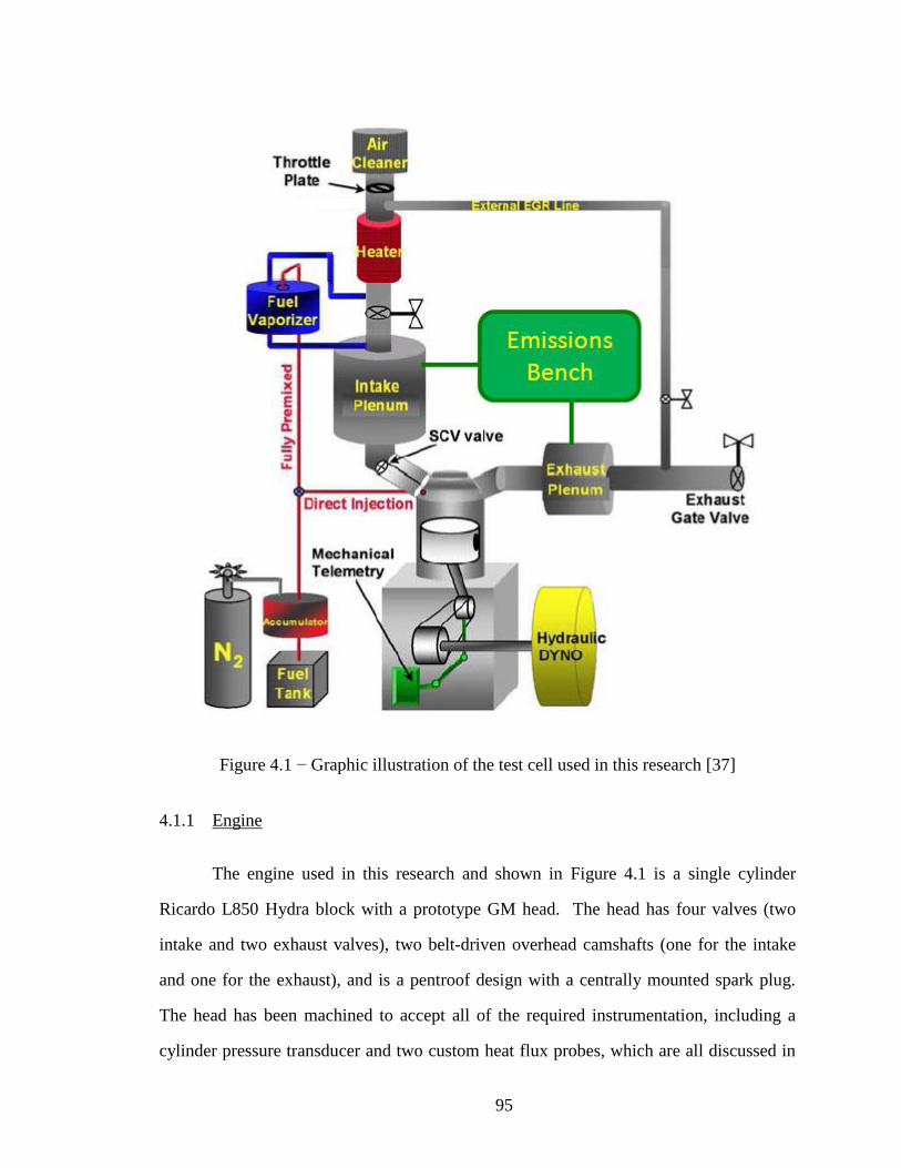
95

Figure 4.1 − Graphic illustration of the test cell used in this research [37]

4.1.1 Engine

The engine used in this research and shown in Figure 4.1 is a single cylinder

Ricardo L850 Hydra block with a prototype GM head. The head has four valves (two

intake and two exhaust valves), two belt-driven overhead camshafts (one for the intake

and one for the exhaust), and is a pentroof design with a centrally mounted spark plug.

The head has been machined to accept all of the required instrumentation, including a

cylinder pressure transducer and two custom heat flux probes, which are all discussed in

96

more detail in subsequent sections. The head was also machined to accept a fuel injector

on the intake side. Coolant and oil flow directly through the head. The piston is a GM

designed piston with an off-center bowl located in a protrusion on the piston top,

designed to mate with the head and create a large squish area. Figure 4.2 is a photograph

of the piston and the head used in this study unless otherwise stated.

Figure 4.2 − Photograph of the head and piston geometries [100]

The cylinder bore is 86 mm. The stroke is 94.6 mm. The head bolts to a cylinder

jug which has passageways for coolant and holds the cylinder liner. The jug in turn bolts

to the crankcase. Spacers were designed between the jug and crankcase to give the

97

desired compression ratio. The target compression ratio was 12.5:1, but it was found that

12.8:1 is a more accurate value to use for the compression ratio. The exhaust camshaft

has a rebreathe lobe to allow hot residuals into the chamber during the intake stroke as

the default configuration is rebreathe or re-induction operation, where the exhaust valve

is opened for a period of time during the intake stroke so that as the piston moves down

and draws in fresh charge, it also inducts some hot exhaust gases as well. Rebreathe

operation is discussed in more detail in Section 4.3.3. Table 2.1 lists some of main

engine specifications. Note that for the valve timings in the table and for the entirety of

this research, 0 crank angle degrees corresponds to TDC combustion.

Table 2.1 − Engine specifications

Engine Type 4 valve, 4 stroke, single cylinder

Bore / Stroke 86 / 94.6 mm

Displacement 0.550 liters

Connecting Rod Length 152.2 mm

Compression Ratio 12.8:1

IVO / IVC 329.5° / -141.5°

Main EVO / EVC 133.5° / -351.5°

Rebreathe EVO / EVC -327.5° / -188.5°

Fuel Type 87 Octane Gasoline (H/C = 1.88)

4.1.2 Fuel Type

The last line of Table 2.1 describes the fuel. There was one, constant fuel used in

this research, since the purpose of this work was not to study fuel chemistry effects. It

was supplied by Haltermann, type HF0072. It is a tightly controlled 87 octane research

grade, unoxygenated gasoline. The H/C for the fuel was 1.88. The lower heating value

98

was 43.129 MJ/kg. Since the combustion chamber deposits were not a main focus of the

current study, a “cleaning dose” (1 oz per gallon) of Techron was added to the gasoline to

mitigate the accumulation of combustion chamber deposit and remove their effect on

combustion.

4.1.3 Dynamometer

The engine’s flywheel is connected to a hydraulic pump/motor assembly, which is

coupled through hydraulic oil to the hydraulic dynamometer. The dynamometer is a

Micro-Dyn computer controlled dynamometer provided by Electro-Mechanical

Associates. The dynamometer is essentially a large electric motor that drives a hydraulic

pump, which is coupled to the pump/motor on the engine’s flywheel. The dynamometer

can either supply positive hydraulic pressure to the pump connected to the engine to

motor the engine, or it can give a negative resistive pressure to control engine load. All

of the data collected in this study was at steady state. In which case, the dynamometer

could effectively hold speed and load.

4.1.4 Emissions Measurements

The emissions bench used in this work is a Horiba Mexa 7100DEGR emissions

analyzer bench. It measures CO, CO2 in the intake and the exhaust, total unburned

hydrocarbon (HC), O2, and NOx emissions. The ratio of CO2 in the intake to CO2 in the

exhaust gives a measurement of the external EGR fraction. In addition to the raw

measurements of exhaust species concentrations, the emissions bench provides two

measurements of the air to fuel ratio; one from a carbon balance of the exhaust products,

and the other from an oxygen balance. Also, from a correlation of exhaust species, the

combustion efficiency is calculated [76, 101]. The emissions bench was a very important

instrument in this research. Even though the exhaust species are not a main focus of this

99

research, the emissions bench gives accurate measurements of the air to fuel ratio and the

combustion efficiency, which are crucial input parameters to the post-processing

discussed in Chapter 2. Figure 4.3 shows a photograph of the Horiba emissions analyzer

bench used in this study. In addition to the species concentration measurements taken by

the exhaust gas analyzers in the emissions bench, there is a wideband Bosch LSU 4.9

lambda sensor connected to an ETAS LA4 lambda meter for measurements of the air to

fuel ratio. No smoke measurements were taken for several reasons. First, the smoke

number for HCCI operation is always very low. Second, as already stated, the emissions

data is not a main focus of this work. Finally, the smoke number is not required by the

post-processing in any way.

Figure 4.3 − Horiba Mexa7100DEGR emission analyzer bench

100

4.2 Instrumentation

4.2.1 Pressure Measurements

The pressure measurements are exceedingly important for this work since the

post-processing analysis relies heavily on accurate pressure data to calculate heat release,

and later a temperature distribution. The post-processed quantities will only be as

accurate as the pressure measurements. Therefore, significant effort was put forth to

ensure accurate and reliable pressure data. The cylinder pressure was measured with a

6125A Kistler, quartz, piezoelectric pressure transducer. There is an intake and exhaust

pressure transducer as well to measure the pressures in the runners. The exhaust pressure

transducer is a Kistler 4045A2 and is located in a water-cooled cooling adapter that keeps

the transducer’s temperature below its maximum temperature of 140 °C. The intake

pressure transducer is a Kistler 4005BA5F. The intake pressure transducer is also cooled

with a water-cooled cooling adapter to keep the transducer’s temperature below its limit

of 200 °C. This is particularly important because some of the data presented in Part II of

this dissertation required very high intake temperatures (above the 200 °C limit of the

transducer). The cooling water was always kept on for both the intake and exhaust

pressure transducers to keep the sensors at a constant low temperature and help ensure

their accuracy. The three pressure signals are collected on a crank angle resolved basis,

which is discussed more in Section 4.2.3.

4.2.2 Heat Flux Probes

Custom heat flux probes in two different locations in the head were used for the

entirety of this research. These heat flux probes measure the surface temperature and

heat flux on a crank angle resolved basis and have been the central focus of much of the

previous research on this engine [37-40]. Each heat flux probe consists of two fast

response thermocouples. One of the thermocouples is located on the surface of the heat

101

flux probe while the other thermocouple is 4 mm behind the surface. The two

thermocouples are separated by a material whose thermophysical properties are well

known. Using the one dimensional transient heat conduction equation, the heat flux can

be calculated by processing the two temperature measurements and using the material

properties. Figure 4.4 is a schematic of the heat flux probe construction provided by the

company’s product information [102].

Figure 4.4 − Heat flux probe schematic [102]

For the purpose of this work, these heat flux probes give accurate measurements

of the surface temperature on a crank angle resolved basis. The surface temperature is

used in the Thermal Stratification Analysis, as discussed in Chapter 2. It is also helpful

to have the heat flux data to study how the perturbation of operating conditions in Part II

affect the measured head side heat flux, but this is not a main focus of this work.

102

4.2.3 Crank Angle Resolved Data Acquisition

Eight data signals are collected on a crank angle resolved basis. The first is the

engine position signal or crank angle signal, which is determined by a 0.5 crank angle

resolution Kistler crank angle encoder, meaning that a data point is collected every 0.5

crank angles (i.e. there are 1440 data points for one 720 crank angle degree engine cycle).

The remaining seven signals are the cylinder pressure, the intake and exhaust manifold

pressures, and the four thermocouple signals from the heat flux probes (two

thermocouples for each heat flux probe, one located on the surface and one 4 mm behind

the surface). The high speed data acquisition system is an AVL Indiset and the software

is AVL Indicom.

In Indicom, the cylinder pressure is filtered using the weakest filter option in

software (a 100 Hz filter), since the raw data will be filtered in the post-processing. The

cylinder pressure is then pegged in software to the intake pressure sensor to compensate

for the drift associated with the dynamic piezoelectric cylinder pressure transducer. The

cylinder pressure will also be pegged again in the post-processing to the intake pressure.

Each day, before collecting data, the intake and exhaust pressure were compared to a

reference barometer at ambient pressure to check their calibrations. Similarly, the heat

flux probe temperatures were calibrated by heating the head to a known temperature and

using a thermistor to measure the room temperature. For every data point, Indicom

records and saves 200 successive cycles.

4.2.4 Time Averaged Data Acquisition

The pressures and heat flux probe temperatures are the only variables collected on

a crank angle resolved basis. The remaining measured quantities are measured on a time

averaged basis. The time averaged data acquisition system is a National Instruments

SCXI 32 channel thermocouple amplifier coupled to LabVIEW software. The

103

parameters that are measured on a time averaged basis are engine speed and load, the

equivalence ratio measured by the lambda sensor and meter, all of the emissions

measurements from the Horiba emissions bench, the mass of fuel from the fuel flow

meter, the fuel pressure, the intake and exhaust temperatures, and the engine coolant and

oil temperatures. Some other temperatures that are monitored in the low speed system

are the fuel vaporizer temperature, the external EGR loop temperature (which needs to be

kept over 100 °C to ensure that the water vapor and unburned hydrocarbon emissions

from the exhaust do not condense out in the EGR loop), and the cooling water

temperatures for the intake and exhaust manifold pressure transducers. All of this data is

collected with LabVIEW, saved on the time averaged data acquisition computer, then

compiled and processed with the corresponding crank angle resolved data file. That is,

for each experimental data point there are two files: one containing the crank angle

resolved data from Indicom, and one containing the time averaged data from LabVIEW.

The time averaged data is collected over the same real time interval that the crank angle

resolved data acquisition system collects its 200 consecutive cycles. 200 engine cycles

will take 12 seconds in real time at 2000 rpm. The time averaged data acquisition is

manually synchronized with the crank angle resolved data acquisition so that the time

averaged data is collected over the same 12 seconds. Since, the crank angle resolved data

collects 200 consecutive cycles, and the time averaged data acquisition system measures

quantities over the same period of time that the crank angle resolved data acquisition is

collecting data, it is extremely important that the engine operation has reached steady

state before the data collection is initiated. Throughout this research, care was taken to

ensure that the engine operation reached steady state before collecting data.

104

4.3 Experimental Capabilities

The previous two sections described the test cell and data collection methodology

for the default configuration. However, during the course of this research, the test cell

and engine were perturbed from the default configuration to test the sensitivities or

effects of different operating conditions on HCCI. This section outlines some of the

capabilities of the test cell that were exploited to study the effects of various operating

conditions.

4.3.1 Intake Heating

At the start of this research, the test cell was equipped with a blanket-type heater,

wrapped around the intake plenum that was only capable of producing 1.3 kW of heating

energy. As a result, it took the intake over twenty minutes to reach 100 °C. More

importantly, the maximum achievable intake temperature was only around 110 °C under

normal flow conditions. This posed a serious problem since some of the experimental

plans included operating without internal residuals and at a lower compression ratio. Both

of which require much higher intake temperatures. To resolve this issue, a 4 kW inline

heater manufactured by Farnam was installed upstream in the intake, in addition to the

1.3 kW blanket heater wrapped around the intake plenum. The controller to both heaters

was a single omega proportional-integral-derivative (PID) controller. The PID function

was necessary since the more powerful inline heater was further upstream of the

measurement location in the intake runner. The PID functionality worked well under

steady state conditions. A fail safe limit control alarm was installed to cut the power to

the heater if the outlet temperature of the heater increased to potentially dangerous levels

for the resistor inside the heater. This limit control alarm was particularly necessary for

the lower engine speeds where the air flow rate was below the minimum recommended

105

flow rate by the manufacturer. The intake heater was placed as close to the intake

plenum as possible, but before the auxiliary loop to the fuel vaporizer.

With the combined 5.3 kW of heating power, the intake was able to reach any

temperature required during the course of the work. The hottest intake temperature that

was required for a data point that was collected was around 280 °C. This is why it was

important to have a water-cooled intake pressure transducer. In addition to the water-

cooled intake pressure transducer, the entire intake system needed to be rebuilt with a

thread sealant that was rated for these high intake temperatures.

4.3.2 Direct Injection versus Fully Premixed Fuel Delivery

The default means of fuel delivery was direct injection. The fuel was pressurized

to approximately 10 MPa in a 2.5 gallon Parker bladder-type accumulator and the fuel

injector is located next to the intake valves, as shown in Figure 4.2. However, the test

cell is equipped with a fuel vaporizer, shown in Figure 4.1, which vaporizes the liquid

fuel in the intake stream. The fuel then has ample time to mix and become homogeneous

in the intake plenum such that a homogeneous, or fully premixed, mixture of fuel and air

is delivered through the intake valves. The vaporizer is a simple device. It is an

insulated aluminum canister with an electrical resistor wrapped around the outside.

Electrical power is directed through the resistor to heat the canister. The temperature of

the fuel vaporizer was kept between 150 °C and 225 °C, which was experimentally

determined to be sufficient for vaporizing the fuel. A fraction of the intake stream was

directed from the inline intake heater described in the previous section through the fuel

vaporizer. It is important to note that in addition to the canister heating, the air that is

sent through the vaporizer is also very hot since it comes from the outlet of the intake

heater. This further helps the vaporization process. A fuel injector (separate from the

one located in the head that injects into the cylinder) injects fuel into the fuel vaporizer,

106

where the heat from the electrical resistor and from the air vaporizes the fuel. The fuel

vapor also gets the chance to begin mixing with the air that is directed through the

vaporizer. However, the mixing is completed in the intake plenum.

Studying the difference between direct injection operation and fully premixing the

fuel and air will help determine how well mixed the fuel-air mixture is under direct

injection and the amount of intake heat that is absorbed by the latent heat of vaporization

with direct injection. Also, sweeps collected under fully premixed operation will remove

the effects of latent heat of vaporization and possible unmixedness, which will be

especially important when the amount of fuel is one of the parameters varying in the

sweep.

4.3.3 Rebreathe versus Positive Valve Overlap Operation

As previously discussed, the default valve strategy employed in this work was

rebreathe operation. Rebreathe, sometimes also called re-induction, is a strategy where

the exhaust valve is reopened a second time during the intake stroke to re-induct a large

amount of hot, burned exhaust gases. Rebreathe and NVO are the two most common

valve strategies for trapping a large amount of internal hot residuals. Each strategy has

their advantages and disadvantages as discussed by [54, 103-105]. Lately, NVO has been

the focus of more attention as it would be easier to execute in a practical engine. In

general, the fixed valve timings, and the somewhat outdated rebreathe strategy, are the

biggest limitation to the current test cell set-up. However, the results are no less valid or

applicable. The capabilities were just somewhat limited.

Figure 4.5 is a diagram of the default rebreathe valve lift profiles showing the

main exhaust event and the second, smaller rebreathe event during the intake stroke. The

amount of hot exhaust gases that are re-inducted into the cylinder depends on the pressure

difference between the intake and exhaust. Generally, the exhaust was kept around 9 kPa

107

higher than the intake pressure and that resulted in a residual gas fraction between 40% to

50% of the cylinder contents by mass.

In addition to the default rebreathe camshafts, there is an exhaust camshaft with

the same lift characteristics as the exhaust camshaft shown in Figure 4.5 except that there

is no second rebreathe event. This camshaft is called the positive valve overlap (PVO)

camshaft and is very similar to the camshafts used in traditional gasoline SI or diesel CI

engines. Operating without the hot residuals will require much higher intake

temperatures, which are now possible thanks to the more powerful intake heater

described in Section 4.3.1. The results from comparing data taken under rebreathe

operation to data collected with the PVO camshafts will show the effect of the internal

residuals on HCCI combustion. Also, sweeps performed with the PVO camshafts can

help clarify the physical effects of various operating conditions by removing the

complication of the internal residuals. For this reason, researchers at Sandia National

Laboratories often refer to this type of HCCI operation as “Pure HCCI” since it simplifies

the results by removing the internal residuals which can cloud the observed trends.

108

Figure 4.5 − Default rebreathe valve lift profile

4.4 Thermal Images of the Test Cell

This chapter describes the test cell equipment, default configuration, and special

capabilities that were taken advantage of during the course of this research. This

subsection offers photographs and infrared thermal images of the test cell while the

engine is running to demonstrate the variety of temperatures that either need to be

managed or will be perturbed to study their effect on the in-cylinder unburned gas

temperature distributions around TDC prior to ignition.

Figure 4.6 is a side-by-side comparison of a photograph of the test cell and a

thermal image of the test cell while the engine was running. The infrared (IR) image

shows the coolant and oil lines that are maintained at a constant temperature to keep the

wall temperature constant. The engine block is at approximately the same temperature as

the coolant and oil lines. Note that the temperature of the engine block is not perfectly

109

constant. Ideally, the engine block would be one constant temperature. The resistor

wrapped around the fuel vaporizer can be seen at an elevated temperature. Also, the

external EGR loop temperature can be seen at a higher temperature due to the heat tape

electric resistor wrapped around the pipe. The exhaust temperature is so hot it appears

white on the infrared image because the temperature is above the upper limit for this

particular arrangement and settings. Lastly, the dynamometer (Dyno) is shown against

the wall giving off some heat to the surroundings to dissipate the energy it absorbs from

the engine.

110

Figure 4.6 − a) Photograph and b) infrared thermal image of the test cell

a)

b)Coolant Tower

and Lines

Fuel Vaporizer

External EGR Loop

Dyno

Exhaust

Engine Block

111

Figure 4.7 is a second infrared thermal image of the engine while running with a

color bar corresponding to the IR measured temperature in Celsius. It is important to

note that the IR thermography is only accurate if the emissivity of the object being

measured is well known and the reflectivity of the object is low. Also, the IR

thermography measures surface temperatures, which are not particularly valuable for any

quantitative analysis in this type of research. Therefore, these images are only useful to

demonstrate the range and variety of temperatures that need to be managed and the color

bar showing the temperature measurements are only intended to serve as an

approximation or estimate of the surface temperature of each component.

In Figure 4.7, the exhaust can be seen as white because it is over the maximum

range of these particular settings, similar to Figure 4.6. The water-cooled exhaust

pressure transducer can be seen (approximately halfway between the head and the

exhaust plenum) acting as a heat sink for the exhaust runner to keep the pressure

transducer below its limit. The engine block appears to range in temperature from around

60 °C to around 95°C. The head is around 95 °C, which is consistent with the target and

measured coolant and oil temperatures. For the most part, the intake side appears much

cooler with the surface temperatures ranging from around 30 °C to 60 °C. This is not

because the gas temperature is in this range, but instead those measured temperatures are

the surface of the insulation that is wrapped around the intake runner. In fact, the

insulation wrapped around the intake plenum and runner has a very reflective surface and

these IR measured surface temperatures are likely only picking up the reflections from

other hot engine parts like the exhaust. There is one part of the intake runner, directly

under the intake plenum, that lost its insulation and the true intake runner metal

temperature can be seen at around 100 °C to 105 °C, which agrees well with the intake

temperature for the baseline operating point.

112

Figure 4.7 − IR thermography of the engine while running

113

CHAPTER 5

EFFECT OF OPERATING CONDITIONS ON THERMAL STRATIFICATION

Part I of this dissertation provided the introduction, motivation, and objective for

this work. A novel post-processing technique for studying thermal stratification in a

fired, metal HCCI engine was proposed, which can calculate an unburned temperature

distribution from heat release. Then, a sensitivity study was done on the constants in the

ignition delay correlation and the Thermal Stratification Analysis was validated against

CFD results and against optically measured temperature distributions. Finally, the test

cell, engine, and instrumentation were described in detail.

In this part of the dissertation (Part II), the TSA technique is used to process

experimental data collected under varying engine operating conditions to study the

effects of varying conditions on the unburned temperature distribution prior to ignition.

The objective is to understand which variables affect the temperature distributions and

HCCI burn rates and why, and to understand which variables do not affect the naturally

occurring thermal stratification and HCCI burn rates.

Constraints of Metal Engine Experiments

Metal engine experiments have their benefits and their drawbacks. The main

advantage is that the results are most applicable to production engines. The metal engine

used in this study closely mimics the combustion chamber and geometry of engines that

are currently in production. In that way, the results that are obtained from these

experiments are exactly what would be seen in a production engine. The general

114

drawback of metal engine experiments is that they can sometimes lack fundamental

understanding. The TSA was developed as part of this work to help further the

capabilities and the degree of fundamental understanding that can be extracted from a

measured pressure trace on a metal engine. But there are still some unknowns and

limitations and many variables that are not directly measured. The experiments are

designed to either prove or disprove a given hypothesis, but with metal engine

experiments, it is almost impossible to change one variable at a time, which can cloud the

results and occasionally make the “why” hard to understand without further investigation

from either optical work or very advanced models.

With this in mind, a number of experiments changing various operating

conditions were conducted as part of this work. From these experiments, observations

can be made based on the results. Then, conjecture and hypothesis are given to explain

why the results are the way they are. Again, the experiments were conducted in such a

way to help narrow the possible explanations, but sometimes, the best that can be done is

hypothesize and recommend to the community further in-depth optical experiments to

determine exactly why the results are the way they are.

5.1 Fuel Preparation

Studying the effect of fuel preparation is particularly important since the analysis

assumes that the mixture is compositionally homogeneous. In that way, this section is

partially to determine if the fuel preparation method affects the unburned temperature

distribution and partially to validate the Compositionally Homogeneous assumption.

Note that if the Compositionally Homogeneous assumption is not valid and there is in

fact a stratification of mixture properties at TDC, this stratification of mixture properties

would be misinterpreted by the TSA as a thermal stratification. That is to say that the

115

only stratification that the analysis can back-calculate is thermal. An equivalence ratio

stratification will appear as a thermal stratification.

5.1.1 Direct Injection versus Fully Premixed Fuel Delivery

Direct injection with the default injection timing (333 CA degrees before TDC

firing) is compared to fully premixed (FP) operation where the fuel and air are mixed

upstream in the fuel vaporizer in Figure 5.1. The comparison is made at three different

operating conditions to see if the difference between fully premixed and direct injection

is sensitive to the operating condition. The black and dashed grey lines labeled “Baseline

- DI” and “Baseline - FP”, respectively, correspond to the baseline conditions (i.e. 2000

rpm, 11 mg of fuel per cycle, rebreathe camshafts with 46% internal residual). The solid

blue and dashed blue-grey lines correspond to a lower fueling rate and low internal

residual operation with the positive valve overlap camshafts (i.e. 2000 rpm, 9.5 mg of

fuel per cycle, around 4% internal residual). The solid red and dashed red-grey lines

correspond to the same lower fueling rate and low internal residual operation as the blue

pair, but with the swirl control valve closed to encourage swirl. For the solid lines

labeled “DI” for Direct Injection, the fuel is directly injected into the cylinder as

described in Chapter 4 at 333 CA degrees before TDC combustion. For the greyer

dashed lines labeled “FP” for Fully Premixed, the fuel is fully premixed in the fuel

vaporizer and allowed to completely mix with the air in the intake plenum. Between each

of the pairs, the only parameter that varied is the fuel preparation (i.e. direct injection

versus fully premixed) and the intake temperature was adjusted to match CA50 phasing.

The intake temperature was decreased by approximately 13-14 K for the fully premixed

operation compared to direct injection because there is an evaporative charge cooling

effect with direct injection that is not present with fully premixed operation.

116

The difference in the temperature distributions between the various operating

condition pairs will be discussed in more detail in subsequent sections. The purpose of

Figure 5.1 is only to study the effect of the fuel preparation method on the unburned

temperature distribution. It can be seen by comparing the pairs in Figure 5.1 that the

fully premixed operation is almost perfectly identical to the direct injection operation.

The very slight shift that does exist between the direct injection and fully premixed data

points is consistent across the varying operating condition pairs. The fully premixed

peaks are a slightly different shape than the corresponding direct injection condition,

which may be caused by a somewhat more homogeneous mixture or it may be caused by

a broader IVC temperature distribution introduced by the evaporative charge cooling. If

the change in the distribution is caused by a less than homogeneous mixture, then the

Compositionally Homogeneous assumption would be invalidated. However, the effect is

very small and could easily be caused by the evaporative cooling effect on the IVC

temperature distribution. Either way, the differences are so small that it gives confidence

that even when directly injecting the fuel, the mixture becomes mostly homogeneous by

TDC and the effect of direct injection at 333 CA degrees before TDC combustion on the

unburned temperature distribution is fairly negligible.

117

Figure 5.1 – Unburned temperature distributions comparing direct injection versus fully

premixed operation

Figure 5.1 also indicates that the mixing between the fresh charge and the residual

is sufficient enough so that the mixture becomes homogeneous by TDC. This fact can be

inferred by recognizing that the relationship between the direct injected and the fully

premixed data points is the same whether the residual gas fraction was high, as in the

baseline black curves, or low, as in the red and blue curves. In the case of the fully

premixed fueling, the fuel is completely premixed with the intake charge only. If the

mixing between the fresh charge and the residuals was insufficient during the intake and

compression strokes, there would regions of mostly intake charge and regions of mostly

exhaust charge, and this would result in a very steep equivalence ratio gradient. The

stratification of equivalence ratio would invalidate the Compositionally Homogeneous

850 900 950 1000 1050 11000

0.002

0.004

0.006

0.008

0.01

0.012

0.014

0.016


Ma

ss P

DF

Baseline - DI

Baseline - FP

Low RGF - DI

Low RGF - FP

Low RGF w/ Swirl - DI

Low RGF w/ Swirl - FP

118

assumption and appear as a thermal stratification. Since the direct injected baseline (high

internal residual) data falls almost perfect on the fully premixed baseline data and the

differences are in a consistent manner with the low residual DI versus FP comparisons, it

can be concluded that the residual and fresh charge are sufficiently well mixed by TDC.

5.1.2 Injection Timing Sweep

To give further insight, an injection timing sweep was performed and the results

were analyzed. Figure 5.2 shows the mass fraction burned curves for the injection timing

sweep with the legend entries corresponding to the injection timing before TDC

combustion. The intake temperature was used to match CA50 phasing and is shown in

the legend in addition to the injection timing. The mass fraction burned curves show that

there are only very subtle changes in the burn characteristics until the injection timing is

delayed to 240 CA degrees before TDC combustion. In fact, 333 CA degrees bTDC, 300

CA degrees bTDC, and 270 CA degrees bTDC lie on top of each other in Figure 5.2 and

are virtually indistinguishable. 240 CA degrees bTDC is also very similar but starts to

show some differentiation from the other three injection timings with the 240 CA degrees

bTDC having a slightly longer burn duration. The longer burn duration indicates that at

240 CA degrees bTDC, the injection timing has delayed to the point where there is not

sufficient time for the fuel-charge mixture to become homogeneous. As a result, there

are some rich pockets and some lean pockets of gas. This equivalence ratio stratification

will tend to lengthen the burn duration because the different regions ignite at different

times. At 210 CA degrees bTDC, the burn duration has lengthened significantly. The

injection timing is so late in the cycle that it is introducing a significant equivalence ratio

stratification.

The required intake temperatures to match CA50 phasing are an indicator of the

steep sensitivity occurring between 240 and 210 CA degrees bTDC as well. For the first

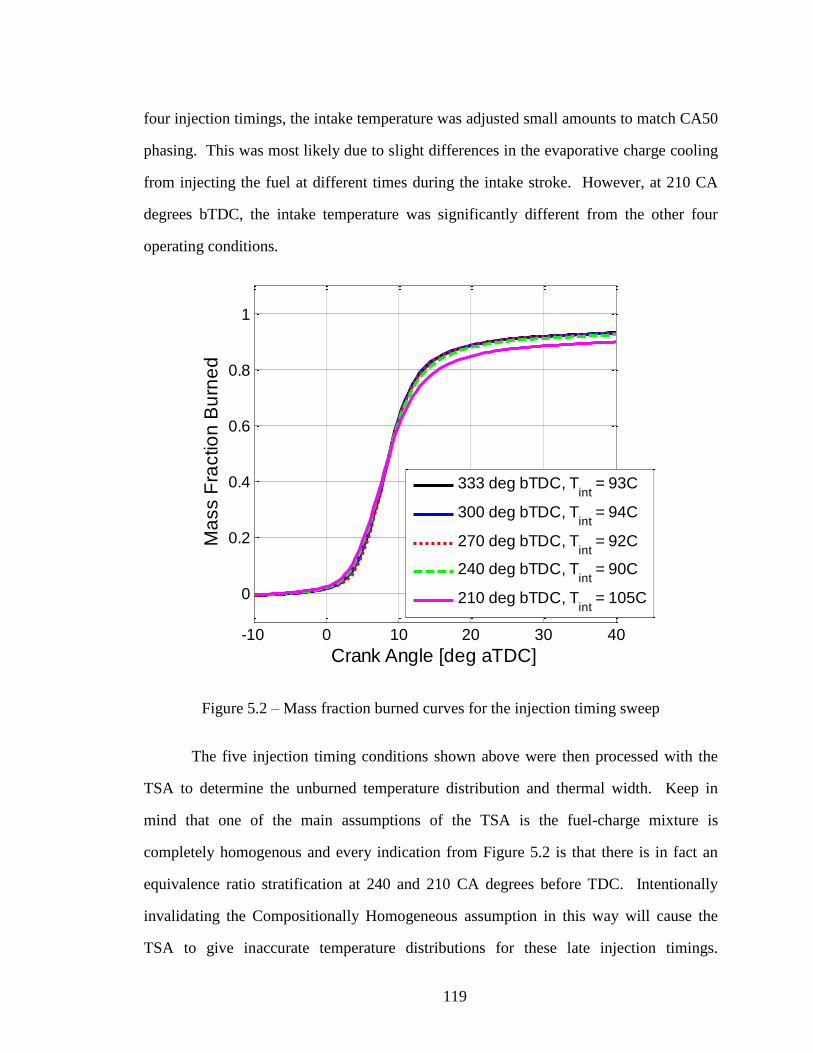
119

four injection timings, the intake temperature was adjusted small amounts to match CA50

phasing. This was most likely due to slight differences in the evaporative charge cooling

from injecting the fuel at different times during the intake stroke. However, at 210 CA

degrees bTDC, the intake temperature was significantly different from the other four

operating conditions.

Figure 5.2 – Mass fraction burned curves for the injection timing sweep

The five injection timing conditions shown above were then processed with the

TSA to determine the unburned temperature distribution and thermal width. Keep in

mind that one of the main assumptions of the TSA is the fuel-charge mixture is

completely homogenous and every indication from Figure 5.2 is that there is in fact an

equivalence ratio stratification at 240 and 210 CA degrees before TDC. Intentionally

invalidating the Compositionally Homogeneous assumption in this way will cause the

TSA to give inaccurate temperature distributions for these late injection timings.

-10 0 10 20 30 40

0

0.2

0.4

0.6

0.8

1


Ma

ss F

ractio

n B

urn

ed

333 deg bTDC, Tint

= 93C

300 deg bTDC, Tint

= 94C

270 deg bTDC, Tint

= 92C

240 deg bTDC, Tint

= 90C

210 deg bTDC, Tint

= 105C

120

However, that is not to say that the temperature distributions are not useful to study. By

assuming the mixture is homogeneous when it is not, any equivalence ratio stratification

will appear to the TSA as a temperature stratification. Figure 5.3 shows the 10% to 90%

and the 25% to 75% thermal widths for the injection timing sweep. The earliest (larger

numbers on the x-axis) three injection timing conditions are within 2% of each other in

terms of thermal width. However, at 240 CA degrees bTDC, the thermal width is 3.5%

larger than the baseline condition on a 10% to 90% basis and 5% larger on a 25% to 75%

basis. At 210 CA degrees bTDC, the thermal width is 12.2% to 12.7% larger than the

thermal width for the baseline injection timing (333 CA degrees bTDC). Realistically,

the thermal width is not varying 12%. Instead it is the equivalence ratio stratification that

increased. But the TSA gives an effective thermal width and in this case the effective

stratification increased 12%.

Figure 5.3 – 10% to 90% and 25% to 75% thermal widths for the injection timing sweep

200 250 300 35040

50

60

70

80

90

100

110

120

Injection Timing [deg bTDC]

Th

erm

al W

idth

at T

DC

[K

]

10% to 90%

25% to 75%

121

The observed relative insensitivity to injection timing when the injection timing is

sufficiently early, followed by a very steep sensitivity once the equivalence ratio

inhomogeneities begin is corroborated by other measured quantities. The intake

temperature is one such measured variable that displayed the same relationship as thermal

width and was discussed above. The efficiencies and emissions also exhibit the same

relationship. Figure 5.4 shows the net indicated fuel conversion efficiency, the

combustion efficiency, and the measured NOx and CO emissions. All four quantities

show the same trend as the thermal width. These results indicate that the mixture is in

fact compositionally homogeneous as long as the injection timing is 270 CA degrees

bTDC or earlier. After 270 CA bTDC, the sensitivity to injection timing is very strong

because there is not enough time for the mixture to become compositionally

homogeneous and there is an equivalence ratio stratification around TDC which greatly

affects the burn characteristics of HCCI.

122

Figure 5.4 – Net indicated fuel conversion efficiency, combustion efficiency, NOx and

CO emissions for the injection timing sweep

5.2 Internal Residual Dilution versus Air Dilution

The effect of internal residuals on the in-cylinder temperature distribution has

recently been investigated by several independent research groups [44, 46, and 49]. Any

practical HCCI engine concept will likely require internal residuals. It is therefore,

immensely important to understand the effects that the internal residuals have on the

unburned temperature distribution and HCCI combustion. The goal of this section is to

explore the effects of internal residuals on the unburned temperature distribution in a

fired, metal HCCI engine.

200 250 300 3500.1

0.2

0.3

0.4

0.5


CO

[%

]

200 250 300 35010

20

30

40

50

60

70


NO

x [p

pm

]

200 250 300 3500.43

0.435

0.44

0.445

0.45

0.455

0.46


Ne

t F

ue

l C

on

ve

rsio

n E

ffic

ien

cy

200 250 300 35094.5

95

95.5

96

96.5

97


Co

mb

ustio

n E

ffic

ien

cy [%

]

123

To study the effect of internal residual, data collected with the baseline rebreathe

configuration is compared to data collected with the positive valve overlap camshafts. As

many variables as possible were held constant while the rebreathe camshafts were

switched for the positive valve overlap camshafts. Keep in mind that the residual gas

fraction with the rebreathe camshafts is around 46-49%, while the residual gas fraction

with the positive valve overlap camshafts is around 3-6%. The fueling rate between the

high and low internal residual points is kept constant. The intake pressure is kept

constant as well. However, the air flow is much higher for the positive valve overlap

operation because the internal residuals are not there to displace the air. That means that

the equivalence ratio is much lower with the air dilute operation. The charge mass

equivalence ratio (sometimes called ϕ’), which is a measure of the ratio of the fuel to the

total charge in the cylinder, is roughly constant. CA50 phasing was kept constant by

adjusting the intake temperature. The intake temperature for the positive valve overlap

operation is between 100 K and 130 K higher than the rebreathe operation because with

the rebreathe camshafts, around 46% of the charge is residual gases which are at exhaust

temperatures. With the positive valve overlap camshafts, all of the required heat for

ignition comes from intake. Therefore, the intake temperatures need to be much higher

under positive valve overlap operation with very little internal residual. The IVC

temperature however is lower for the positive valve overlap operation than for the

rebreathe operation by around 30 K for two reasons. First, without the internal residual

the gamma of the mixture is higher, meaning that the IVC temperature can be lower and

the same TDC temperature will be attained. The second reason that the IVC temperature

is lower without the internal residuals is that the ignition delay is shorter with a purely air

dilute mixture. The shorter ignition delay means that for a constant combustion phasing

the TDC temperature can be lower.

Two different fueling rates were compared: 11 mg per cycle and 9 mg per cycle.

Figure 5.5 first compares the mass fraction burned curves for the four operating

124

conditions. The mass fraction burned curves show that the dashed PVO (air dilute) data

points have a faster burn rate than their internal residual dilute counterparts. This could

be due to several reasons. First, it could be that the mixture is not well mixed and that

there is a stratification of mixture properties that cause the distribution to ignite at

different times. While this is possible, it is unlikely because Figure 5.1 strongly suggests

that the mixing between the fresh charge and the residual is sufficient enough so that the

mixture is fairly homogeneous by TDC (see discussion above). Second, some

researchers believe that the oxygen concentration plays a role in the energy release rates

of HCCI. This theory however, is inconsistent with the conceptual picture of HCCI as a

sequential autoignition of cooler and cooler regions with the cooler, later-phased regions

being compressed by the energy release from the hotter, earlier-phased regions. It is

therefore inconsistent with the assumptions of the TSA and the TSA will not help to

determine if the oxygen concentration affects burn rates. The third potential reason for

the faster energy release rates with the air dilute mixtures is that the internal residuals are

introducing a thermal stratification, which staggers the autoignition of the regions with

different temperatures and results in a slower global energy release rate. The TSA will

help to determine the effect of the internal residual gas fraction on the unburned

temperature distribution.

Figure 5.5 also shows that the higher fueling rate data has a faster burn especially

later in the event, even though CA50 phasing is matched. This is due to the physical

chain reaction of burned gases compressing the unburned gas, which is amplified with the

higher fueling rate, as discussed in Chapter 1. In addition to the accelerated physical

chain reaction, the bulk temperature after combustion is higher for the higher fueling rate

data, which results in better hydrocarbon burn up later in the combustion event,

explaining the difference in combustion efficiency between the 9 mg and 11 mg data.

125

Figure 5.5 – Mass fraction burned curves for high and low residual gas fraction

comparison at 11 mg and 9 mg of fuel per cycle

The data shown in Figure 5.5 was then processed with the TSA to determine the

unburned temperature distribution prior to ignition. Figure 5.6 shows the TSA-

determined distributions at TDC for this internal residual gas fraction comparison. The

unburned temperature distributions at either fueling rate show that rebreathe operation is

in fact spreading the temperature distribution compared to air dilute operation with the

positive valve overlap camshafts. This finding is in great agreement with the findings by

Rothamer et al. [46], who optically showed that internal residuals from negative valve

overlap operation greatly broadens the temperature distribution compared to positive

valve overlap operation. The distribution is broader for the larger internal residual gas

fraction for two main reasons. The first reason is that there is a much greater

stratification of temperature at and around intake valve closing with a large amount of

-10 0 10 20 30 40

0

0.2

0.4

0.6

0.8

1


Ma

ss F

ractio

n B

urn

ed

11mg Rebreathe

11mg PVO

9mg Rebreathe

9mg PVO

126

internal residual. The second is that the ignition delay is longer with the residuals, which

means that for a given combustion phasing, the TDC temperatures need to be higher.

This can be seen by comparing the location of the hottest, leading edge of the

distributions in Figure 5.6. The higher maximum TDC temperature spreads the

distribution, since the cold side of the distribution is relatively unchanged.

Interestingly, the difference in thermal width, with the addition of internal

residuals, appears more significant at the higher fueling rate in Figure 5.6. One

possibility is that at the higher fueling rate, the exhaust temperature and therefore internal

residual temperature is higher. A lower intake temperature can then be used to achieve

the same TDC temperature. However, if the internal residuals introduce a temperature

distribution at IVC, it is reasonable to assume that the thermal width of the IVC

temperature distribution increases as the difference in temperature between the residual

and fresh charge increases, as is the case with the higher fueling rate points. The other

somewhat unexpected observation in Figure 5.6 is that there is an effect of increasing

fueling rate, but the trend reverses depending on if there is residual or fresh charge. That

is to say that the 9 mg rebreathe condition has a higher peak than the 11 mg rebreathe

condition. However, the 9 mg PVO point has a lower peak than the 11 mg PVO point.

This indicates that there are at least two different effects of changing fueling rate, and one

of which depends on whether there is a significant internal residual fraction. The

hypothesis is that the increasing residual temperature and decreasing intake temperature

with increasing fueling rate is the effect that depends on the residual gas fraction. The

other effect of fueling rate on the distribution is that increasing equivalence ratio shortens

the ignition delay and lowers the required TDC temperatures for a given combustion

phasing. The lower maximum TDC temperature tightens the distribution for a given wall

temperature. These effects will be discussed and further examined in Section 5.6 which

explores fueling rate effects in more detail. The impact of internal residuals on the

reactivity of the mixture and the higher maximum TDC temperature required to match

127

combustion phasing is another contributing factor for why the width of the distribution

increases with the presence of internal residuals. Again, the influence of ignition delay

on the temperature distributions will be explained in more detail in the subsequent

sections.

Figure 5.6 – Unburned temperature distributions at TDC for high and low internal

residual gas fraction comparison at 9 mg and 11 mg of fuel per cycle

Figure 5.7 is a bar graph of the 25% to 75% thermal widths for the four data

points shown in Figure 5.5 and 5.6. Examining the thermal widths shows the same trend

that was previously discussed; the rebreathe data shows a broader distribution than the air

dilute positive valve overlap data. At 11 mg of fuel per cycle, the rebreathe thermal

width is 14.5% larger than the PVO thermal width. At 9 mg of fuel per cycle, the

rebreathe thermal width is 11.0% larger than the PVO thermal width. The higher percent

800 850 900 950 1000 1050 11000

0.005

0.01

0.015


Ma

ss P

DF

11mg Rebreathe

11mg PVO

9mg Rebreathe

9mg PVO

128

increase in thermal width for the 11 mg comparison reiterates the trend seen in Figure

5.6. Again, the difference between the 11 mg and the 9 mg points in general will be

discussed more in Section 5.6.

Figure 5.7 – 25% to 75% thermal widths for the internal residual gas fraction study

Figure 5.8 shows the 10% to 90% thermal widths, instead of the 25% to 75%

thermal widths, shown in Figure 5.7. It is interesting to note that on the 10% to 90%

basis, the rebreathe distribution is 12.2% wider for the 11mg comparison and 11.6%

wider for the 9 mg comparison. While an increase in thermal width of 11.6% or 12.2%

may not seem significant, it is important to understand how a change in the temperature

distribution of this magnitude affects the burn duration. For HCCI combustion

researchers looking to expand the operating range and control the energy release rates, it

is much more important to study the changes in the burn duration rather than the

temperature distribution. In this case, the effect on the burn duration is much more

129

profound. At 11 mg of fuel per cycle, the rebreathe operation 10% to 90% burn duration

is 33.9% longer than PVO and the rebreathe 10% to 90% burn duration is 47.5% longer

than the PVO burn duration at 9 mg of fuel per cycle.

Figure 5.8 – 10% to 90% thermal widths for the internal residual gas fraction study

The results from Section 5.2 show that the addition of internal residuals greatly

broadens the temperature distribution and lengthens the burn rate, while the inferred

conclusion from the direct injection versus fully premixed comparisons is that the internal

residuals are sufficiently mixed to provide near-homogeneous mixture compositionally

around TDC. That is to say that the presence of internal residuals has only a small effect

on the compositional stratification but a significant effect on the thermal stratification.

These findings are in excellent agreement with Kodavasal [49] who computationally

found that the primary means of the burn duration lengthening from NVO is an increased

thermal stratification and that the compositional effects of NVO are insignificant. He

130

observed a 30% increase in burn duration from the presences of internal residauls, which

is very similar to the 33.9% increase that is presented in this work.

5.3 Intake Temperature Sweep

An intake temperature sweep was performed where all the variables were held

constant except for the intake temperature and the combustion phasing. This sweep will

help to determine the effects of varying intake temperature and combustion phasing on

the unburned temperature distribution. The engine speed for this intake temperature

sweep was 2000 rpm. The rebreathe cams were used and the internal residual gas

fraction was around 47%. 11.8 mg of fuel per cycle was directly injected. The intake

temperature varied from 105 °C to 96 °C to 89 °C and finally to 83 °C. Figure 5.9 shows

the resulting mass fraction burned curves corresponding to the 4 intake temperature

points. As the intake temperature decreases, the combustion phasing retards from 5.9 CA

aTDC to 11.1 CA aTDC.

131

Figure 5.9 – Mass fraction burned curves for the intake temperature sweep

These data points were then processed with the TSA and the unburned

temperature distributions are shown in Figure 5.10. As the intake temperature, and IVC

temperature increases, the maximum TDC temperature (leading, hottest edge of the

distributions) increases as well. However, since the wall temperature is staying roughly

constant over the sweep, the cold side of distributions is relatively unaffected. In fact, for

three of the four data points, the curves lie perfectly on top of each below a temperature

of about 975 K. The point that does not exactly align with the other three is the lowest

intake temperature and latest phased data point. Chapter 3 demonstrated how the validity

of the analysis decreases with later phasing because the Fast Chemistry and the No

Mixing assumptions break down. It is possible that this is why the lowest intake

temperature point is somewhat of an outlier. In general, the trend is such that the cold,

near-wall region of the distribution is not affected by the increase in intake temperature.

-10 0 10 20 30 40

0

0.2

0.4

0.6

0.8

1


Ma

ss F

ractio

n B

urn

ed

Tint

= 105C

Tint

= 96C

Tint

= 89C

Tint

= 83C

132

However, the hot leading edge of the distribution increases with intake temperature,

which results in a spreading of the distribution. It is not clear from this one sweep if the

shear temperature difference between the wall and the core is the only reason for the

broadening of the distribution with increasing intake temperature or if the advancing

combustion phasing also plays a role in spreading the temperature distribution. It is

possible that the unburned temperature distribution is sensitive to changes in combustion

phasing as well. Section 5.4 will explore the effects of combustion phasing in more

detail.

Figure 5.10 – Unburned temperature distributions for the intake temperature sweep

Figure 5.11 shows the 10% to 90% and 25% to 75% thermal widths for the 4

points presented in Figure 5.10. Note that the thermal widths are plotted against intake

temperature but could have just as easily been plotted against CA50 phasing and the trend

would have been just as strong. The trend of either the 10% to 90% thermal width or

850 900 950 1000 1050 11000

0.002

0.004

0.006

0.008

0.01

0.012

0.014


Ma

ss P

DF

Tint

= 105C

Tint

= 96C

Tint

= 89C

Tint

= 83C

133

25% to 75% thermal width are very linear, with increasing intake temperature and

advanced combustion phasing causing larger thermal widths. The 10% to 90% and 25%

to 75% thermal widths of the lowest intake temperature point are 19.3% and 17.7% wider

than the thermal widths of the highest intake temperature point.

Figure 5.11 – Thermal widths for the intake temperature sweep

Whether the cause of the spread in the distribution is from the temperature

difference between the core and the wall or from advancing combustion phasing, the

effect on HCCI is same. The wider distribution for the higher intake temperature and

earlier phased data points help to slow the positive feedback loop of HCCI energy release

that was discussed in Chapter 1. That is to say that the increase in burn rates with

advancing combustion phasing would be much larger if the temperature distribution was

not spreading at the same time. Without this spreading of the temperature distribution

355 360 365 370 375 38040

50

60

70

80

90

100

110

Intake Temperature [K]

Th

erm

al W

idth

at T

DC

[K

]

Tint - 10% to 90%

Tint - 25% to 75%

134

with increasing intake temperature and advancing combustion phasing, it is possible that

HCCI would not be viable because HCCI would be even more difficult to control.

5.4 Premixed Positive Valve Overlap Combustion Phasing Study

The intake temperature sweep above showed that as the intake temperature

increased and combustion phasing advanced, the temperature distribution broadened

significantly. It was unclear, however, if the effect was due to increasing intake

temperature or advancing combustion phasing, or a combination of the two. The goal of

this section is to help determine which of these effects is causing the temperature

distribution to widen. In the case that both variables have an effect on the temperature

distribution, hopefully this section will help to determine the extent that the effect is

caused by one variable or the other.

To determine if intake temperature or combustion phasing is affecting the

temperature distribution, an experiment was designed where combustion phasing could

be changed with intake temperature, or with increasing equivalence ratio, and therefore

increasing the reactivity of the mixture. To increase the combustion phasing with

equivalence ratio, the mass of fuel injected per cycle was increased while the air flow and

intake pressure were held constant. Since it is unclear if, or how much, the direct

injection and evaporative cooling of the fuel introduces a temperature stratification

during the intake stroke and at IVC, the experiment was performed using the upstream

fuel vaporizer so that the intake charge is completely premixed. This is particularly

important since the mass of fuel will be varying, which would mean varying effects of the

direct injection event on the intake temperature distribution. Additionally, to remove the

concerns over residual gas mixing with fresh charge and potentially introducing a

stratification of temperature at IVC, the PVO camshafts were used in this combustion

phasing study. Again, it is critical to remove the effect of internal residual on the IVC

135

temperature when the mass of fuel is varying because the residual temperature will

increase with fueling rate and the effect would not be constant over the sweep. The goal

is to remove all of the effects of increasing fueling rate except the increasing reactivity

and shorter ignition delays.

Figure 5.12 shows the mass fraction burned curves for the five intake temperature

sweep data points and the five equivalence ratio points. The baseline condition is 9 mg

of fuel per cycle, an equivalence ratio of 0.306, and an intake temperature of 235 °C.

Note that the red line and the dashed red line are two different data points, but the

conditions are the same for both. That is to say they are both baseline data points for

these sweeps and they help to show the repeatability of the data, and later, of the analysis.

Each independent sweep has five points where the variable being swept is varied in both

directions of the baseline condition. Also, note that the CA50 combustion phasings of

each color pair matches. This way, each five point sweep has the same five CA50

combustion phasings but a different variable was used in each sweep to attain each

combustion phasing. Both phasing sweeps show a slower burn rate as combustion

phasing retards due to the instantaneous piston sweep and its effect on the physical chain

reaction of HCCI, as discussed in Chapter 1. However, the equivalence ratio sweep also

has the variable fueling rate effect, again discussed in Chapter 1, where the higher fueling

rate points (higher equivalence ratio points) have a much faster burn rate due to the

positive feedback loop and the burn gases having more potential to compress the

unburned gases, accelerating the physical chain reaction of HCCI.

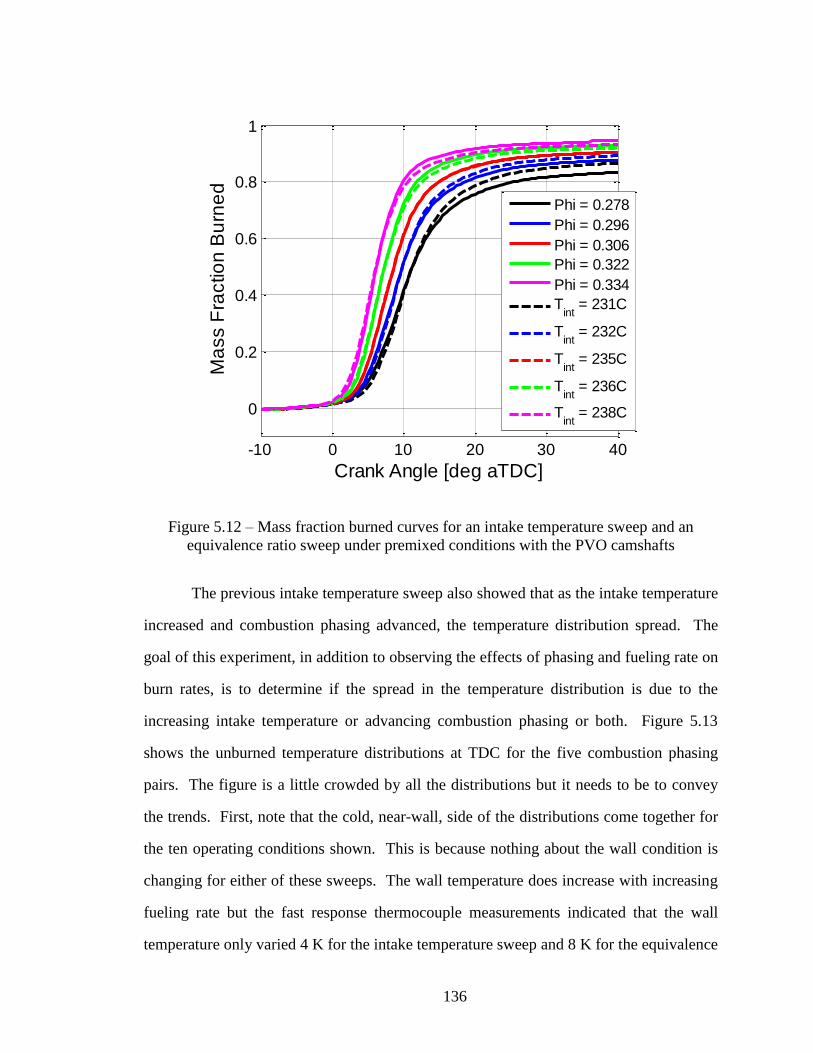
136

Figure 5.12 – Mass fraction burned curves for an intake temperature sweep and an

equivalence ratio sweep under premixed conditions with the PVO camshafts

The previous intake temperature sweep also showed that as the intake temperature

increased and combustion phasing advanced, the temperature distribution spread. The

goal of this experiment, in addition to observing the effects of phasing and fueling rate on

burn rates, is to determine if the spread in the temperature distribution is due to the

increasing intake temperature or advancing combustion phasing or both. Figure 5.13

shows the unburned temperature distributions at TDC for the five combustion phasing

pairs. The figure is a little crowded by all the distributions but it needs to be to convey

the trends. First, note that the cold, near-wall, side of the distributions come together for

the ten operating conditions shown. This is because nothing about the wall condition is

changing for either of these sweeps. The wall temperature does increase with increasing

fueling rate but the fast response thermocouple measurements indicated that the wall

temperature only varied 4 K for the intake temperature sweep and 8 K for the equivalence

-10 0 10 20 30 40

0

0.2

0.4

0.6

0.8

1


Ma

ss F

ractio

n B

urn

ed

Phi = 0.278

Phi = 0.296

Phi = 0.306

Phi = 0.322

Phi = 0.334

Tint

= 231C

Tint

= 232C

Tint

= 235C

Tint

= 236C

Tint

= 238C

137

ratio sweep. Chapter 6 studies the wall conditions in more detail, but an 8 K change in

the wall temperature is not enough to affect the temperature distribution. In addition to

the cold sides of the distributions, the hot sides of the distributions lie on top of each

other for the equivalence ratio sweep. For the equivalence ratio sweep, the intake

temperature is constant. Since the fuel is premixed upstream and the residual gas fraction

is low, the IVC temperature is roughly constant, resulting in an approximately constant

maximum TDC temperature over the equivalence ratio sweep. The gamma of the

mixture will change slightly with the variation of equivalence ratio. However, that effect

was roughly canceled by the small change in wall temperature and heat transfer. On the

other hand, the maximum TDC temperature for the intake temperature sweep increases

linearly with intake temperature, as previously shown in Figure 5.10. This increase

spreads the temperature distribution, giving a larger thermal width for the higher

maximum TDC temperatures. However, the temperature distributions for the

equivalence ratio sweep spread as well, although to a slightly lesser extent than the intake

temperature sweep, even though the maximum TDC temperature is roughly constant

across the sweep. This indicates that combustion phasing alone plays a role in the

temperature stratification, where the earlier phased cases have a wider temperature

distribution. Increasing intake temperature spreads the distribution as well, due to the

increasing maximum TDC temperature with a constant cold near-wall region. Both

variables play a role in creating the temperature distribution.

A hypothesis as to why the combustion phasing alone affects the temperature

distribution is given in the following discussion. Dec has shown that the temperature

distribution develops throughout the compression process [43-45] with a great deal of the

stratification being introduced over the last 30 crank angle degrees before TDC. He

speculates that the turbulent transport caused by the compression process mixes the cold

near-wall regions with the hot core gases to produce the stratification at TDC. The

turbulent transport is particularly affective at and around TDC when the distances

138

between the core and the wall are shortened. These images demonstrated how the

temperature distribution changes over the compression process due to turbulence and heat

transfer with the relatively cold walls. The theory as to why the unburned temperature

distribution narrows after TDC is that the effect of turbulence on the distribution is

highest at TDC where the in-cylinder turbulence is highest. After TDC, the turbulent

fluctuations decreases and the temperature of the mixture is allowed to become slightly

more homogeneous. Dec’s images show that the ensemble averaged temperature

distributions are significantly narrower than the individual cycle’s distribution because

the random turbulent motion is averaged out and only the boundary layers remain, which

has a much smaller effect on broadening the distribution [45]. Dec’s original PLIF

images did in fact show the same effect seen in this phasing study; the temperature

distribution narrows after TDC [43] (see Figure 1.9). However, his more recent, and

likely more accurate, results did not show this effect [45]. Instead, the thermal

stratification increased after TDC and reached a maximum in the expansion stroke. He

speculated that cold gases leaving the crevices once the cylinder pressure begins to

decrease along with growing boundary layers cause the distribution to broaden [45]. In

[45], Dronniou and Dec decomposed the thermal stratification into the cycle-to-cycle

mean, which is representative of the boundary layers, and the fluctuating component,

which is representative of the thermal stratification in the core and, they say, is most

relevant to HCCI burn rates. They observed that the fluctuating component does in fact

peak at TDC, but the total thermal stratification increases after TDC due to an increase in

the mean stratification from growing boundary layers and out-gassing from crevices. The

peak of the fluctuating component at TDC agrees well with the findings presented here

for the combustion phasing study. Peterson et al. saw a similar effect to Dronniou and

Dec in an optical engine where the temperature distributions broaden during expansion

due to out-gasing and growing boundary layers [106]. These results were obtained on a

motored cycle and the results may be different for a fired cycle. Also, the phasing study

139

shown here is a finer resolution than either of the optical investigations discuss above (i.e.

Dec’s optical data was only taken every 10 crank angle degrees). Therefore, it is possible

that the diminishing turbulence after TDC causes the temperature distribution to narrow.

At this point however, this is only a hypothesis.

140

Figure 5.13 – Unburned temperature distributions at TDC for an intake temperature

sweep and an equivalence ratio sweep under premixed conditions with the PVO

camshafts

900 950 1000 10500

0.002

0.004

0.006

0.008

0.01

0.012

0.014

0.016


Ma

ss P

DF

Phi = 0.278

Phi = 0.296

Phi = 0.306

Phi = 0.322

Phi = 0.334

Tint

= 231C

Tint

= 232C

Tint

= 235C

Tint

= 236C

Tint

= 238C

a)

1000 1010 1020 1030 1040 1050 1060 10700

0.002

0.004

0.006

0.008

0.01

0.012

0.014

0.016


Ma

ss P

DF

b)

141

Figure 5.14 shows the thermal width for the equivalence ratio and intake

temperature sweeps plotted against combustion phasing. There is a very strong trend or

correlation of combustion phasing with thermal width. If the thermal widths for the

sweeps were plotted against intake temperature, the intake temperature sweep would have

a strong correlation but the equivalence ratio sweep would not. Also note that the slope

is steeper for the intake temperature sweep than for the equivalence ratio sweep because

for the intake temperature sweep both the advancing combustion phasing and the

increasing maximum TDC temperature are causing the distribution to spread, whereas for

the equivalence ratio sweep, only the advancing combustion phasing is causing the

distribution to spread. For the equivalence ratio sweep, the earliest phased data point has

a 7.0% wider 10% to 90% thermal width than the latest phased point. Comparing the

same bookend points of the intake temperature sweep gives a 14.7% difference. This

suggests that of the 14.7% variation of 10% to 90% thermal width seen over the intake

temperature sweep, about half of the change is from the advancing combustion phasing

and half is from the increasing maximum TDC temperature.

If the same comparisons are done on the 25% to 75% thermal widths, the

equivalence ratio sweep exhibits an 11.4% total change and the intake temperature sweep

exhibits a 16.5% total change. Now, a larger percent of the total change of the intake

temperature sweep is due to the advancing combustion phasing rather than the increasing

maximum TDC temperature. This makes intuitive sense because the increasing

maximum TDC temperature will have a larger effect on the 10% to 90% thermal widths

than the 25% to 75% thermal widths being that the maximum TDC temperature is on one

of the tails of the distribution. It is also interesting to note that the advancing combustion

phasing plays a bigger role in the bulk 25% to 75% of the charge than for the 10% to

90%, which include more of the behavior of the tails.

142

Figure 5.14 – Thermal widths for the equivalence ratio (Phi) and intake temperature (Tint)

sweeps plotted against combustion phasing

5.5 Positive Valve Overlap Swirl Study

Since the intake temperature sweep and the combustion phasing study suggested

that turbulence may play a role in determining the in-cylinder unburned temperature

distribution prior to ignition, it was desired to study the effect of swirl on the unburned

temperature distribution. The intake runner has a “swirl control valve” (labeled SCV in

Figure 4.1). By closing the swirl control valve, the intake charge is directed through the

port that is tangential to the chamber to encourage swirl. Under rebreathe operation, it is

unclear how much swirl would be induced because the directed intake charge motion

might be attenuated by the residuals that are also inducted into the cylinder during the

intake stroke. For this reason, the swirl study was performed using the positive valve

overlap camshafts, so that any directed intake charge motion will continue into the

6 7 8 9 10 11 1240

50

60

70

80

90

100

110

CA50 [deg aTDC]

Th

erm

al W

idth

at T

DC

[K

]

Phi - 10% to 90%

Phi - 25% to 75%

Tint

- 10% to 90%

Tint

- 25% to 75%

143

cylinder. By closing the swirl control valve with the PVO camshafts, swirl inside the

cylinder will be induced. The level of swirl was never directly measured because the

head and intake runner were never tested on a flow bench. Therefore, the swirl ratio with

and without the swirl control valve closed is not specifically known.

Two intake temperature sweeps were collected to study the impact of swirl on the

unburned temperature distributions. First, an intake temperature was collected with the

swirl control valve completely open. Second, the swirl control valve was completely

closed and an intake temperature sweep was collected matching the combustion phasing

to each point in the previous intake temperature sweep. The mass fraction burned curves

for the two different intake temperature sweeps are shown in Figure 5.15. The mass

fraction burned curves show that with the swirl control valve closed the burn durations

are slightly longer. This result is consistent with the findings by Sjöberg et al. [95]. The

lengthening of the burn duration appears fairly uniform across the range of combustion

phasings. Also, for the latest phased condition, the combustion efficiency is higher with

the swirl control valve closed. This trend does not continue for the other combustion

phasings. Being the latest phased case, the combustion efficiency is the lowest. It is

possible that the swirl helps to mix the cold hydrocarbons from near the wall into the

core. Another possibility is that the swirl helps mix the burned gases and unburned gases

increasing the combustion efficiency.

Somewhat strangely, the required intake temperatures with swirl are lower than

without swirl. The exact reason for this phenomenon is not well understood. It was

observed that this was only the case when the swirl control valve was completely closed.

If the swirl control valve was only partially closed, the required intake temperature to

match combustion phasing increased, as is expected. Unique and unexpected behavior

has been observed on this engine before when the swirl control valve is completely

closed and it was attributed to a storage effect in the intake runner [107]. When the swirl

control valve is completely closed, it seals off a section of the intake runner. The intake

144

valve still opens and closes as it would and has access to this sealed section of the intake

runner. It is possible that this storage effect is responsible for the lower intake

temperatures with swirl. Alternatively, it may be due to the decreased residence time of

the intake charge in the intake port and runner resulting in a higher temperature at the

intake valve for a given measured intake runner temperature.

Figure 5.15 – Mass fraction burned curves for the PVO intake temperature sweeps with

and without swirl

Figure 5.16 shows the unburned temperature distributions for the mid-phased

condition (solid and dashed red lines) in Figure 5.15. Figure 5.16 shows that swirl

greatly affects the unburned temperature distribution. The distribution is wider with a

lower peak with swirl compared to without swirl. This shows that the unburned

temperature distributions are affected by directed intake charge motion and in-cylinder

turbulence.

0 10 20 30 40

0

0.2

0.4

0.6

0.8

1


Ma

ss F

ractio

n B

urn

ed

Tint

= 234C

Tint

= 236C

Tint

= 238C

Tint

= 240C

Tint

= 242C

Swirl, Tint

= 230C

Swirl, Tint

= 231C

Swirl, Tint

= 233C

Swirl, Tint

= 235C

Swirl, Tint

= 238C

145

Figure 5.16 – Unburned temperature distributions with and without swirl for the mid-

phased condition

Only one of the five CA50 phasing pairs from Figure 5.15 is shown in Figure

5.16 to simplify the plot. The mid-phased condition is fairly representative of all five

data points. The 10% to 90% and 25% to 75% thermal widths for the five CA50 pairs are

shown in Figure 5.17. The thermal width is larger with swirl for all of the cases except

for the 10% to 90% thermal widths for the latest phased condition, which showed the

unique combustion efficiency behavior in Figure 5.17. The most interesting fact that

Figure 5.17 helps illuminate is that the relative change in the thermal width caused by

swirl increases with advanced combustion phasing. Figure 5.18 shows the percent

change in thermal width from the addition of swirl. The earlier combustion phasings

show a larger percent change from the addition of swirl. These results give credence to

940 960 980 1000 1020 1040 10600

0.002

0.004

0.006

0.008

0.01

0.012

0.014

0.016

0.018


Ma

ss P

DF

Tint

= 238C

Swirl, Tint

= 233C

146

the hypothesis that the broadening of the temperature distribution with earlier combustion

phasing is due to increased turbulence.

Figure 5.17 – 10% to 90% and 25% to 75% thermal widths for the swirl study

6 7 8 9 10 11 1240

50

60

70

80

90

100

110

CA50 [deg aTDC]

Th

erm

al W

idth

at T

DC

[K

]

No Swirl - 10% to 90%

No Swirl - 25% to 75%

Swirl - 10% to 90%

Swirl - 25% to 75%

147

Figure 5.18 – Percent change of thermal width with the addition of swirl as a function of

combustion phasing

This section demonstrated that swirl can be used to affect the unburned

temperature distribution. Figure 5.18 showed that the temperature distribution could be

broadened by almost 5% with the addition of swirl. In this way, swirl could be used as a

control variable to help control the unburned temperature distribution and control HCCI

burn rates. However, increasing the in-cylinder turbulence through the addition of swirl

also increases the heat transfer losses. Figure 5.19 shows the net indicated fuel

conversion efficiency for the intake temperature sweeps with and without swirl. The net

indicated fuel conversion efficiency with swirl is between 1.2 to 1.8 percentage points, or

2.8% to 4%, below the corresponding points without swirl. The smallest decrease in

efficiency occurs at the latest phased condition where the increase in combustion

efficiency helps to offset the increase in heat transfer losses.

6 7 8 9 10 11 12-5

-4

-3

-2

-1

0

1

2

3

4

5

CA50 Phasing [deg aTDC]

Pe

rce

nt C

ha

ng

e in

Th

erm

al

Wid

th w

ith

Sw

irl [%

]

10% to 90%

25% to 75%

148

Figure 5.19 – Net indicated fuel conversion efficiency for the intake temperature sweeps

with and without swirl

Observation of the Coefficient of Variation

Studying and understanding the sources of cyclic variability is not a focus of this

work. However, a large amount of data was collected in the course of this research and

any observations that can be made from collecting or processing the data will be given to

offer as much insight as possible, even if an in-depth understanding of all of the

observations cannot be provided. In addition to the observation about the effect of

completely closing the swirl control valve on the required intake temperature to match

combustion phasing, it was observed that the coefficient of variation of indicated mean

effective pressure decreased a noticeable amount with swirl compared to without swirl.

The lower COV could be due to the increased organization of the intake charge motion

6 7 8 9 10 11 120.405

0.41

0.415

0.42

0.425

0.43

0.435

0.44

0.445

0.45

CA50 [deg aTDC]

Ne

t F

ue

l C

on

ve

rsio

n E

ffic

ien

cy

No Swirl

With Swirl

149

trapping a more consistent amount of mass. Otherwise, it could be due to the increased

gas velocities with half the intake flow area resulting in a more consistent trapped mass.

5.6 Premixed Positive Valve Overlap Compensated Load Sweep

A compensated load sweep is a sweep of the mass of fuel injected per cycle, and

therefore the engine load, while the intake temperature is adjusted to keep combustion

phasing constant (i.e. the intake temperature is used to compensate for the effects of

changing fueling rate on combustion phasing). In an HCCI engine with a large amount of

internal residuals, as the fueling rate increases, the intake temperature will have to

decrease to keep the combustion phasing constant. This inverse relationship between

fueling rate and intake temperature is caused by two main reasons. First, as the fueling

rate increases, the mixture gets richer, increasing the reactivity of the mixture. The intake

temperature needs to decrease to offset the decreasing ignition delay. The second main

reason for the inverse relationship between the intake temperature and fueling rate is that

as the fueling rate increases, the residual temperature increases. The intake temperature

needs to decrease to compensate for the increasing internal residual temperature. With a

high residual strategy, this is the dominant effect, whereas with a low internal residual

strategy, the varying ignition delay is the dominant effect.

In this section, the effects of inversely varying the intake temperature and fueling

rate on the unburned temperature distribution are examined. The main purpose of this

sweep is to determine the effects of varying ignition delay and varying the maximum

TDC temperature. Previous sections hinted that the ignition delay and mixture reactivity

may impact the unburned temperature distribution because the maximum TDC

temperature will need to inversely vary with ignition delay to keep the combustion

phasing constant. To eliminate the residual mixing effects and the increasing internal

residual temperature, the sweep was performed with the PVO camshafts and the internal

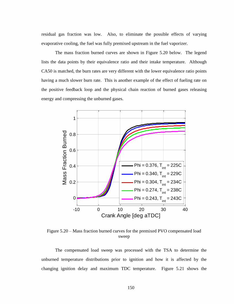
150

residual gas fraction was low. Also, to eliminate the possible effects of varying

evaporative cooling, the fuel was fully premixed upstream in the fuel vaporizer.

The mass fraction burned curves are shown in Figure 5.20 below. The legend

lists the data points by their equivalence ratio and their intake temperature. Although

CA50 is matched, the burn rates are very different with the lower equivalence ratio points

having a much slower burn rate. This is another example of the effect of fueling rate on

the positive feedback loop and the physical chain reaction of burned gases releasing

energy and compressing the unburned gases.

Figure 5.20 – Mass fraction burned curves for the premixed PVO compensated load

sweep

The compensated load sweep was processed with the TSA to determine the

unburned temperature distributions prior to ignition and how it is affected by the

changing ignition delay and maximum TDC temperature. Figure 5.21 shows the

-10 0 10 20 30 40

0

0.2

0.4

0.6

0.8

1


Ma

ss F

ractio

n B

urn

ed

Phi = 0.376, Tint

= 225C

Phi = 0.340, Tint

= 229C

Phi = 0.304, Tint

= 234C

Phi = 0.274, Tint

= 238C

Phi = 0.243, Tint

= 243C

151

unburned temperature distributions at TDC for the compensated load sweep. The cold,

near-wall region of the distributions overlap since the wall condition is not significantly

changing. However, as the equivalence ratio decreases and the reactivity of the mixture

decreases, the maximum TDC temperature must increase to keep the combustion phasing

constant. This results in a spreading of the distribution. Figure 5.21 illustrates that the

reactivity of the mixture indirectly affects the temperature distribution by requiring an

change in the maximum TDC temperature. The maximum TDC temperature is really a

dependent variable in a fired engine. Based on the ignition delay and reactivity of the

mixture, the combustion phasing determines what maximum TDC temperature is

required. Therefore, the ignition delay and mixture reactivity and combustion phasing

determine the width of the temperature distribution.

Figure 5.21 – Unburned temperature distributions at TDC for the compensated load

sweep

800 850 900 950 1000 1050 11000

0.002

0.004

0.006

0.008

0.01

0.012

0.014

0.016


Ma

ss P

DF

Phi = 0.376, Tint

= 225C

Phi = 0.340, Tint

= 229C

Phi = 0.304, Tint

= 234C

Phi = 0.274, Tint

= 238C

Phi = 0.243, Tint

= 243C

152

Figure 5.22 shows the 10% to 90% and the 25% to 75% thermal widths for the

compensated load sweep. The 10% to 90% and 25% to 75% thermal widths show the

same trend that was visually seen in Figure 5.21; the thermal width increases with

decreasing equivalence ratio and increasing intake and maximum TDC temperatures.

The lowest equivalence ratio operating condition has a 20% larger 10% to 90% thermal

width than the highest equivalence ratio point, which is a significant change to the

unburned temperature distribution. The 25% to 75% shows a slightly lower sensitivity

with the lower equivalence ratio operating condition being 12.6% wider than the highest

equivalence ratio operating condition. The higher sensitivity of the 10% to 90% is

because the reason for the spreading distribution is the sliding maximum TDC

temperature, which is inherently on one of the tails of the distribution.

Figure 5.22 – Thermal widths for the compensated load sweep

0.25 0.3 0.35 0.440

50

60

70

80

90

100

110

Equivalence Ratio

Th

erm

al W

idth

at T

DC

[K

]

10% to 90%

25% to 75%

153

5.7 Chapter Summary

To summarize, this chapter presents the first implementation of the TSA to

experimental data. A large amount of data was collected under varying operating

conditions to determine the effects of engine operating conditions on the in-cylinder

unburned temperature distribution and HCCI burn rates. It was found that the differences

between direct injection and fully premixing the fuel in the intake stream were small. An

injection timing sweep was studied to determine the injection timing limit, after which

compositional inhomogeneities exist around TDC. Next, the impact of the internal

residual gas fraction on the unburned temperature distribution was studied. The presence

of internal residuals and the valve strategy had a significant impact on the unburned

temperature distribution, where rebreathe operation resulted in a much wider temperature

distribution. Then, the effects of intake temperature and combustion phasing were

studied. It was found that increasing intake temperature broadens the distribution by

increasing the maximum TDC temperature while leaving the wall region unaffected.

Additionally, combustion phasing itself impacts the thermal width, where earlier

combustion phasing leads to a broader distribution. It was speculated that the increasing

thermal width with advancing combustion phasing is due to the increasing turbulent

charge motion as TDC is approached. To test the theory about advancing combustion

phasing and observe the effect of turbulence on the unburned temperature distribution, a

swirl study was performed at varying combustion phasing. The results showed that

adding swirl broadened the temperature distribution and that the spread of the distribution

was slightly larger at earlier combustion phasings. Lastly, it was observed that increasing

the equivalence ratio while keeping combustion phasing constant caused the distribution

to narrow because the higher equivalence ratio conditions have shorter ignition delays

and require lower maximum TDC temperatures.

154

CHAPTER 6

EFFECT OF WALL CONDITIONS ON THERMAL STRATIFICATION

Chapter 5 used the Thermal Stratification Analysis to explore the effect of

operating conditions on the unburned temperature distribution prior to ignition in a fired

HCCI engine. The key findings were that combustion phasing alone affects the

temperature distribution where the earlier phased data showed a wider distribution.

Additionally, the temperature location of the maximum TDC temperature relative to the

cold side of the distribution determines the width of the distribution. Therefore, variables

that influence the maximum TDC temperature, like mixture reactivity, can also change

the width of the temperature distribution.

In Chapter 5, every effort was made to hold the wall conditions constant. In this

chapter, the effects of wall conditions on the unburned temperature distribution are

explored. These wall conditions include wall temperature and piston surface material.

6.1 Wall Temperature

The wall temperature can be controlled by varying the coolant temperature.

Previous studies showed that the measured wall temperature changed proportionally with

coolant temperature [38]. Varying the coolant, and wall, temperatures alone will result in

different combustion phasings, because the wall temperature plays a role in determining

the IVC temperature through heat transfer losses across the valve and during the intake

stroke. In a high residual engine, the wall temperature also influences the heat transfer

losses during combustion and the expansion and exhaust strokes, which will affect the

155

residual gas temperature. To keep combustion phasing constant, the intake temperature

needs to be adjusted. This type of sweep is called a compensated coolant temperature

sweep because the intake temperature is used to compensate for the coolant temperature’s

effects on combustion phasing.

The sweep below is a compensated coolant temperature sweep, (the intake

temperature and coolant temperature sweep were inversely varied). As the coolant

temperature decreases from 95 °C to 67 °C, the intake temperature increased from 105 °C

to 155 °C. The mass fraction burned curves, shown in Figure 6.1, for the four points lie

perfectly on top of each other. This result seems to indicate that the effects of coolant

temperature are only during the intake stroke, since intake temperature can be used to

completely compensate for coolant temperature and there are no differences to the burn

rates.

Figure 6.1 – Mass fraction burned curves of the compensated coolant temperature sweep

-10 0 10 20 30 40

0

0.2

0.4

0.6

0.8

1


Ma

ss F

ractio

n B

urn

ed

Tint

= 105C, Tcool

= 95C

Tint

= 126C, Tcool

= 83C

Tint

= 143C, Tcool

= 74C

Tint

= 155C, Tcool

= 67C

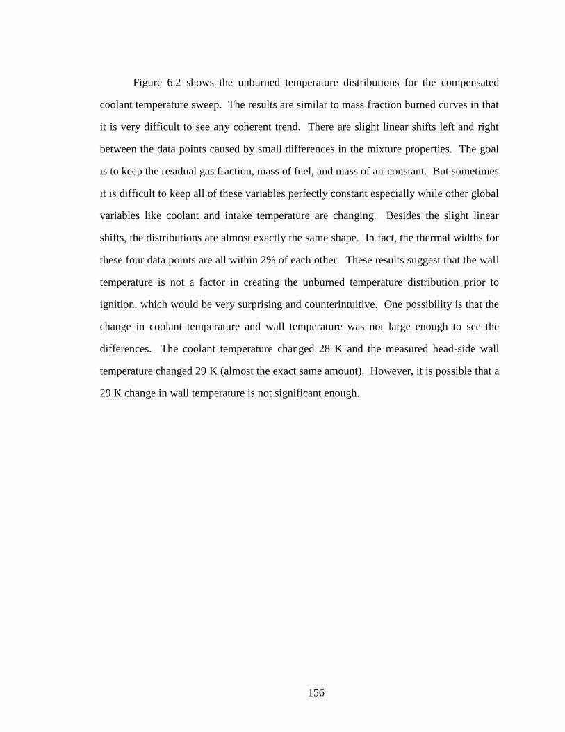
156

Figure 6.2 shows the unburned temperature distributions for the compensated

coolant temperature sweep. The results are similar to mass fraction burned curves in that

it is very difficult to see any coherent trend. There are slight linear shifts left and right

between the data points caused by small differences in the mixture properties. The goal

is to keep the residual gas fraction, mass of fuel, and mass of air constant. But sometimes

it is difficult to keep all of these variables perfectly constant especially while other global

variables like coolant and intake temperature are changing. Besides the slight linear

shifts, the distributions are almost exactly the same shape. In fact, the thermal widths for

these four data points are all within 2% of each other. These results suggest that the wall

temperature is not a factor in creating the unburned temperature distribution prior to

ignition, which would be very surprising and counterintuitive. One possibility is that the

change in coolant temperature and wall temperature was not large enough to see the

differences. The coolant temperature changed 28 K and the measured head-side wall

temperature changed 29 K (almost the exact same amount). However, it is possible that a

29 K change in wall temperature is not significant enough.

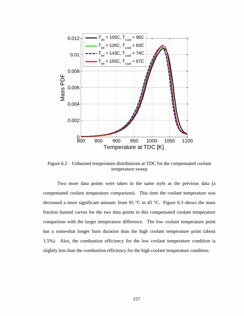
157

Figure 6.2 – Unburned temperature distributions at TDC for the compensated coolant

temperature sweep

Two more data points were taken in the same style as the previous data (a

compensated coolant temperature comparison). This time the coolant temperature was

decreased a more significant amount: from 95 °C to 45 °C. Figure 6.3 shows the mass

fraction burned curves for the two data points in this compensated coolant temperature

comparison with the larger temperature difference. The low coolant temperature point

has a somewhat longer burn duration than the high coolant temperature point (about

1.5%). Also, the combustion efficiency for the low coolant temperature condition is

slightly less than the combustion efficiency for the high coolant temperature condition.

800 850 900 950 1000 1050 11000

0.002

0.004

0.006

0.008

0.01

0.012


Ma

ss P

DF

Tint

= 105C, Tcool

= 95C

Tint

= 126C, Tcool

= 83C

Tint

= 143C, Tcool

= 74C

Tint

= 155C, Tcool

= 67C

158

Figure 6.3 – Mass fraction burned curves for the compensated coolant temperature

comparison with the larger temperature difference

Figure 6.4 shows the unburned temperature distributions for the compensated

coolant temperature comparison. With the larger temperature difference between the

coolant temperature and the intake temperature, the expected trend can begin to be seen.

There is a little more mass near the wall for the low coolant temperature condition and

the distribution is slightly broader than the high coolant temperature condition. In fact,

the thermal width for the low coolant temperature condition is about 3% larger than the

thermal width for the high coolant temperature condition.

-10 0 10 20 30 40

0

0.2

0.4

0.6

0.8

1


Ma

ss F

ractio

n B

urn

ed

Tint = 96C, Tcool = 95C


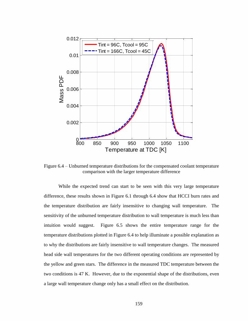
159

Figure 6.4 – Unburned temperature distributions for the compensated coolant temperature

comparison with the larger temperature difference

While the expected trend can start to be seen with this very large temperature

difference, these results shown in Figure 6.1 through 6.4 show that HCCI burn rates and

the temperature distribution are fairly insensitive to changing wall temperature. The

sensitivity of the unburned temperature distribution to wall temperature is much less than

intuition would suggest. Figure 6.5 shows the entire temperature range for the

temperature distributions plotted in Figure 6.4 to help illuminate a possible explanation as

to why the distributions are fairly insensitive to wall temperature changes. The measured

head side wall temperatures for the two different operating conditions are represented by

the yellow and green stars. The difference in the measured TDC temperature between the

two conditions is 47 K. However, due to the exponential shape of the distributions, even

a large wall temperature change only has a small effect on the distribution.

800 850 900 950 1000 1050 11000

0.002

0.004

0.006

0.008

0.01

0.012


Ma

ss P

DF



160

Figure 6.5 – Unburned temperature distributions for the compensated coolant temperature

comparison over the entire range of temperatures

These results are very surprising and counterintuitive, but repeatable on this

engine. It is possible that these results are specific to this engine and it could be that the

present of internal residuals is the driving force behind the in-cylinder thermal

stratification in this engine with rebreathe operation. The results may be different with

positive valve overlap operation. Also, the style of the experiment, where the intake

temperature is used to compensate for coolant temperature may be influencing the results.

If the coolant temperature was changed alone, there may be an impact on the thermal

stratification. This is an area that needs further exploration in the future.

400 600 800 10000

0.002

0.004

0.006

0.008

0.01

0.012


Ma

ss P

DF



161

6.2 Ceramic Coatings

The previous section showed that the wall temperature can affect the temperature

distribution but it is a much more subtle relationship than one would assume once the

changes to combustion phasing are compensated for with intake temperature. This

section explores the effect of piston surface material on HCCI burn rates and the

unburned temperature distribution. To do so, four ceramic coated pistons were tested in a

similar way as the baseline aluminum piston. As many variables were kept constant as

possible from one piston to the next. For example, adding ceramic coating to the pistons

would increase the compression ratio and cloud the results. It would be difficult to

determine if the results were caused by the different ceramic coatings or the varying

compression ratio. To help resolve the issue, the target thickness for the ceramic coating

was machined off the top of the piston. With that said, the flame-spray method did not

accurately deposit the target amount of material. Table 6.1 shows the target and actual

thickness of the ceramic coatings, along with the estimated material properties. In Table

6.1, Piston #1 is the baseline aluminum piston and is the basis for comparisons with all of

the ceramic coated pistons. Piston #2 is a magnesium zirconate coating over the entire

combustion chamber surface of the piston. Piston #3 is the same magnesium zirconate

coating as Piston #2. However, the coating is only applied to the periphery of the piston

or the squish region and the bowl is left uncoated. Piston #4 is the converse of Piston #3;

the bowl of the piston is coated with the same magnesium zirconate coating as Piston #2,

while the periphery of the piston is left uncoated. By comparing Piston #2 through #4,

the effects, if any, of spatial variations in the ceramic coating can be understood. Piston

#5 is a somewhat different ceramic (an yttrium stabilized zirconium oxide) to determine

if the varying material properties impacts HCCI combustion differently. All of the

ceramic coated pistons can be compared to the baseline metal piston to observe the

differences between the aluminum and ceramic coated pistons. Also, the ceramic coated

162

pistons can be compared amongst themselves to observe the impact of the subtle

differences of the coatings on HCCI burn rates and the unburned temperature

distributions.

Table 6.1 – Ceramic coated piston test matrix

Nominal Thermal

Conductivity

Nominal Thermal

Diffusivity Material Coverage

Target Thickness

Actual Compression

Thickness Ratio

Piston #

[μm] [μm] [W/m-K] [*10

-6

m2/s]

1 Aluminum - - - 12.8:1 215 84

2 Magnesium

Zirconate Full

Coverage 150 496 13.33 1.5 0.75-1.31

3 Magnesium

Zirconate Periphery

Only 150 390 12.99 1.5 0.75-1.31

4 Magnesium

Zirconate Bowl Only

150 361 12.94 1.5 0.75-1.31

5

Yttrium Stabilized Zirconium

Oxide

Full Coverage

150 294 13.02 2.25 0.6

The compression ratio variation is small but not negligible and could still be

potentially large enough to cloud the results. The pistons were tested regardless of the

compression ratio difference. Each piston was tested and compared to the metal piston at

the baseline conditions. The intake temperature was used to adjust for changes to

combustion phasing. That is to say that each of the ceramic pistons greatly changed the

combustion phasing by decreasing the heat transfer losses during the intake and

compression strokes (and in this case, by increasing the compression ratio). The intake

temperature needed to be lowered in all cases for the ceramic coated pistons to match

CA50 phasing to the baseline aluminum piston. The goal of this experiment however, is

not to determine the effect on combustion phasing. Instead, the goal is to determine the

163

effects of ceramic coated pistons on HCCI burn rates and the unburned temperature

distribution. Therefore, the intake temperature was used to remove the combustion

phasing effects.

Figure 6.6 shows the mass fraction burned curves for the five different pistons.

The mass fraction burned curves show that once the intake temperature is used to adjust

for the differences in heat transfer and the increasing compression ratio, the difference

between the burn characteristics are very subtle. Most of the differences occur within the

last 25%, where the ceramic pistons have a somewhat faster burn rate and are able to

reach a slightly higher combustion efficiency (it is very difficult to see in the figure).

Chapter 7 will show that higher compression ratios generally lead to lower combustion

efficiency because the expansion happens faster and the bulk temperature drops more

quickly, inhibiting unburned hydrocarbon consumption late in the process. In this case,

the pistons with the marginally higher compression ratio end up with slightly higher

combustion efficiencies because the surface material effect overpowers the compression

ratio effect. The ceramic coated pistons are able to increase the combustion efficiency by

increasing wall temperature and increasing the temperature of the gas near the wall,

which is largely responsible for determining the combustion efficiency of a particular

cycle. The difference from the metal piston to the ceramic coated pistons is barely

detectable. Distinguishing between the ceramic coatings is impossible. If there are

differences between the ceramic coatings, the techniques employed in this work are not

specific or precise enough to sense any distinction.

164

Figure 6.6 – Mass fraction burned curves for the piston surface material comparison

The data collected with various ceramic coated pistons was then processed with

the TSA and the resulting temperature distributions are shown in Figure 6.7. The

unburned temperature distributions at TDC give the same impression as the mass fraction

burned curves in Figure 6.6. Largely, the piston surface material does not have a

significant impact on the unburned temperature distribution and the HCCI burn rates.

Again, there are very subtle differences between the distributions. All of the ceramic

coated pistons are below the baseline metal (black) line in Figure 6.7. The higher surface

temperature of the ceramic coated pistons is able to raise the temperature of the mass near

the wall and shift some of the mass from near the wall to higher temperatures, resulting in

the higher combustion efficiency. This caused the global distribution to be narrower, but

-10 0 10 20 30 40

0

0.2

0.4

0.6

0.8

1


Ma

ss F

ractio

n B

urn

ed

Metal, Tint

= 106C

Full MgZr, Tint

= 77C

Periphery, Tint

= 92C

Bowl, Tint

= 96C

Yttria, Tint

= 90C

165

only marginally. The thermal widths of the ceramic pistons compared to the baseline

metal piston are all between 0 and 3.2% smaller.

Figure 6.7 – Unburned temperature distributions for the piston surface material

comparison

While the effect of the ceramic coated pistons on HCCI burn rates and the

unburned temperature distribution was smaller than expected, the effect of the ceramic

coated pistons on HCCI in general is not insignificant. Keep in mind that the intake

temperature needed to be adjusted a large amount to match combustion phasing. The

ceramic pistons absolutely have an effect on HCCI combustion phasing. It is only the

effect on the burn rate and the unburned temperature distribution when the open-cycle

effects are compensated for with intake temperature that is minimal. The same is true for

wall temperature variations. Changing wall temperature alone has a very significant

800 850 900 950 1000 1050 11000

0.002

0.004

0.006

0.008

0.01

0.012

0.014


Ma

ss P

DF

Metal, Tint

= 106C

Full MgZr, Tint

= 77C

Periphery, Tint

= 92C

Bowl, Tint

= 96C

Yttria, Tint

= 90C

166

effect on HCCI combustion. However, these results show that when intake temperature

is used to compensate for the changes in combustion phasing, the effects of wall

temperature on the HCCI burn rate and the unburned temperature distribution are small.

6.3 Chapter Summary

This chapter describes the efforts that were made to understand the impact of wall

conditions on the unburned temperature distribution. The results showed a surprising

insensitivity to wall temperature and piston surface material. Higher wall temperatures

did result in higher combustion efficiencies and slightly less mass near the wall in the

temperature distribution. However, the impact on the temperature distribution for large

changes in wall temperature or material was very subtle. It was speculated that the

insensitivity to wall conditions is due to the exponential functional shape near the wall.

167

CHAPTER 7

EFFECT OF ENGINE GEOMETRY ON THERMAL STRATIFICATION

The effect of operating conditions like intake temperature, combustion phasing,

fueling rate, wall temperature, and internal residual gas fraction on the unburned

temperature distribution and HCCI burn rates were explored in the previous two chapters.

The objective of this chapter is to attempt to observe the effects of the global engine

geometry variables on the unburned temperature distribution and HCCI burn rates.

It is much more difficult to change a global variable like compression ratio or

engine geometry. Collecting just one data point at a different compression ratio requires

completely deconstructing the engine, adding a spacer between the crankcase and the jug,

and rebuilding the engine with the new clearance volume. For this reason, this chapter

only contains three different operating conditions: the first is a default compression ratio

of 12.8:1 and the default piston geometry (off-center bowl); the second is a lower

compression ratio of 10.2:1 with the default piston geometry; and the third operating

condition is the low compression ratio with a flat top piston. From these three operating

conditions, two comparisons can be made. First, the default 12.8:1 compression ratio is

compared to lower compression ratio of 10.2:1, both with the same default piston

geometry. Later, the flat top piston is compared to the default off-center bowl piston at

the lower compression ratio. For each comparison, the TSA is used to help understand

the influence of engine geometry on the unburned temperature distribution. The purpose

of the first comparison is to determine the effects of only changing compression ratio on

the unburned temperature distribution. The goal of the second comparison is to

understand the impact of changing piston geometry on the unburned temperature

168

distribution while holding the compression ratio constant. It was incredibly difficult to

perfectly match the compression ratio for the two different pistons, because a new spacer

needed to be machined to exactly match the clearance volume of one piston to the other.

The low compression ratio case with the off-center bowl piston was 10.2:1. For the flat

top piston, the compression ratio was 10.1:1.

7.1 Compression Ratio

To study the effect of varying compression ratio on the unburned temperature

distribution, the default 12.8:1 compression ratio was compared to a lower compression

ratio of 10.2:1. This comparison was made by disassembling and rebuilding the engine

with a spacer between the crankcase and the jug so that the clearance volume would be

larger. As many variables were held constant as possible (engine speed, fueling rate,

internal residual fraction), while the intake temperature was used to match combustion

phasing. The intake temperature needed to increase a substantial amount for the lower

10.2:1 compression ratio compared to the 12.8:1 compression ratio. The difference in

intake temperature was 136 °C.

Figure 7.1 shows the mass fraction burned curves for the two different

compression ratios. The burn characteristics are very similar with only slight differences

between the two compression ratios. The burn duration of the low compression ratio case

is marginally longer than the high compression ratio case. The combustion efficiency is

higher for the lower compression ratio data because the bulk temperature remains

elevated for longer into the cycle. Eng showed that hydrocarbon consumption continues

as long as the bulk temperature is above 1400 K [108]. The bulk temperatures for the

compression ratio comparison are shown in Figure 7.2. The bulk temperature for the low

compression ratio condition stays above 1400 K for 17 CA degrees longer than the high

compression ratio condition. Besides the marginal difference in the burn duration and the

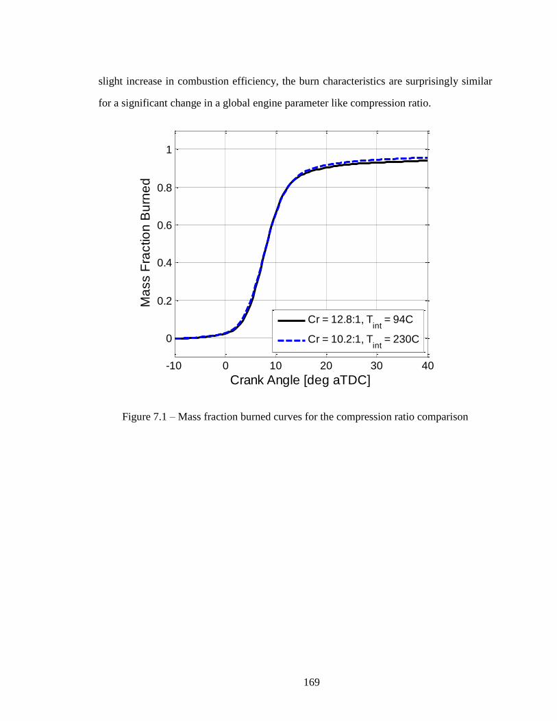
169

slight increase in combustion efficiency, the burn characteristics are surprisingly similar

for a significant change in a global engine parameter like compression ratio.

Figure 7.1 – Mass fraction burned curves for the compression ratio comparison

-10 0 10 20 30 40

0

0.2

0.4

0.6

0.8

1


Ma

ss F

ractio

n B

urn

ed

Cr = 12.8:1, Tint

= 94C

Cr = 10.2:1, Tint

= 230C

170

Figure 7.2 – Bulk temperatures for the compression ratio comparison

The default and low compression ratio operating conditions were processed with

the Thermal Stratification Analysis to determine the effect of compression ratio on the

unburned temperature distribution. Figure 7.3 shows the unburned temperature

distributions for the default and low compression ratio cases. Although the burn

characteristics were very similar in terms of the mass fraction burned curves, the

unburned temperature distributions for the default and low compression ratio data are

noticeably different. The leading, hottest edge of the low compression ratio distribution

is about 12 K hotter than the default compression ratio case. This is due to the effect of

pressure on ignition delay. The lower compression ratio has a lower pressure before

ignition and therefore requires a higher temperature to match combustion phasing. The

peak of the low compression ratio distribution is lower than the default compression ratio

and the width is larger. The cold, near-wall regions of the distributions coincide. The

-120 -80 -40 0 40 80 120400

600

800

1000

1200

1400

1600

1800

2000

2200


Bu

lk T

em

pe

ratu

re [K

]

Cr = 12.8:1, Tint

= 94C

Cr = 10.2:1, Tint

= 230C

171

10% to 90% and 25% to 75% thermal widths of the low compression ratio distribution

are 1.4% and 3.5% larger than the thermal widths for the default compression ratio

configuration, respectively. The hypothesis as to why the unburned temperature

distribution is sensitive to compression ratio is that the ignition delay of the mixture is

impacted by the varying pressure at ignition. The effect of changing ignition delay at

constant combustion phasing was previously seen in the compensated load sweep and the

internal residual gas fraction comparison. In the case of compression ratio, the ignition

delay is affected by the difference in pressure prior to ignition, rather than changing

mixture composition. The maximum TDC temperature needs to compensate for the

lengthening ignition delay at lower compression ratios to match combustion phasing and

the resulting distribution is broader. The compression ratio comparison is another

example of the width of the temperature distribution being affected by changing the

ignition delay.

172

Figure 7.3 – Unburned temperature distributions for the compression ratio comparison

7.2 Piston Geometry

The objective of this section is to determine what, if any, are the effects of

changing piston geometry on the unburned temperature distribution prior to ignition.

Two different pistons were tested while making every effort to keep the compression

ratio constant. The default off-center bowl piston geometry was compared to a flat top

piston. Figure 7.4 is a photograph of the two pistons showing the significant difference

in geometry. The default piston has an off-center bowl located in a protrusion from the

piston top designed to match the pentroof geometry of the cylinder head and create a

large squish region around the periphery of the piston. For the flat top piston, the surface

is very close to being completely flat. There is a very shallow wide bowl centrally

located but the majority of the surface area of the piston is flat. To match the

800 850 900 950 1000 1050 11000

0.002

0.004

0.006

0.008

0.01

0.012

0.014


Ma

ss P

DF

Cr = 12.8:1, Tint

= 94C

Cr = 10.2:1, Tint

= 230C

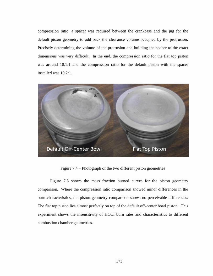
173

compression ratio, a spacer was required between the crankcase and the jug for the

default piston geometry to add back the clearance volume occupied by the protrusion.

Precisely determining the volume of the protrusion and building the spacer to the exact

dimensions was very difficult. In the end, the compression ratio for the flat top piston

was around 10.1:1 and the compression ratio for the default piston with the spacer

installed was 10.2:1.

Figure 7.4 – Photograph of the two different piston geometries

Figure 7.5 shows the mass fraction burned curves for the piston geometry

comparison. Where the compression ratio comparison showed minor differences in the

burn characteristics, the piston geometry comparison shows no perceivable differences.

The flat top piston lies almost perfectly on top of the default off-center bowl piston. This

experiment shows the insensitivity of HCCI burn rates and characteristics to different

combustion chamber geometries.

174

Figure 7.5 – Mass fraction burned curves for the piston geometry comparison

The data from the two piston geometries was processed with the TSA and the

resulting unburned temperature distributions at TDC are shown in Figure 7.6. Although

no perceivable differences existed in the mass fraction burned curves, there are

differences in unburned temperature distributions for the two piston geometries. The flat

top piston has a slightly lower peak, wider distribution, and hotter maximum TDC

temperature. The 10% to 90% and 25% to 75% thermal widths for the flat top piston are

2.3% and 1.5% larger than the off-center bowl piston. If the observed differences are

attributed to the varying piston geometry, the trend would be in a counterintuitive way.

Intuition might suggest that the flat top piston would have a narrower temperature

distribution due to the more favorable surface area to volume ratio, the decreased heat

transfer losses, and potentially, the decreased turbulence near TDC because the off-center

bowl piston has a significant squish region which the flat top piston lacks. The trend seen

-10 0 10 20 30 40

0

0.2

0.4

0.6

0.8

1


Ma

ss F

ractio

n B

urn

ed

Off-Center Bowl

Flat Top

175

in the data is in the opposite direction; the flat top piston has a broader distribution than

the off-center bowl piston, albeit only slightly. It is possible that the effects of piston

geometry are counterintuitive. It is more likely that the small differences seen in the

distributions are attributed to the small change in compression ratio and/or experimental

variability. The flat top piston has a somewhat lower compression ratio than the default

off-center bowl geometry piston. Figure 7.3 shows the same change to the distribution as

Figure 7.6, suggesting that the difference in compression ratio is responsible for the

spread in the distribution in Figure 7.6. Figure 7.3 shows a larger variation of thermal

widths, but the variation of compression ratio is much larger as well. The goal was to

keep the compression ratio constant. Although a good effort was made and the

compression ratios are very similar, the small difference in compression ratio is most

likely responsible for the slight difference in the unburned temperature distributions at

TDC. The results seem to suggest that the effects, if any, of changing the piston

geometry on HCCI burn rates and the unburned temperature distribution prior to ignition

are small.

176

Figure 7.6 – Unburned temperature distributions for the piston geometry comparison

The unburned hydrocarbon emissions and the combustion efficiency for the three

different piston configurations are shown in Figure 7.7. The combustion efficiency

increases, and the unburned hydrocarbons decrease, with decreasing compression ratio

due to the elevated bulk temperature later in the expansion stroke, as previously

discussed. It also appears that changing from the off-center bowl piston to the flat top

piston has the same effect as decreasing compression ratio. This can be attributed to the

more favorable surface area to volume ratio with the flat top piston compared to the off-

center bowl piston as well as the slight difference in compression ratio.

800 850 900 950 1000 1050 11000

0.002

0.004

0.006

0.008

0.01

0.012

0.014


Ma

ss P

DF

Off-Center Bowl

Flat Top

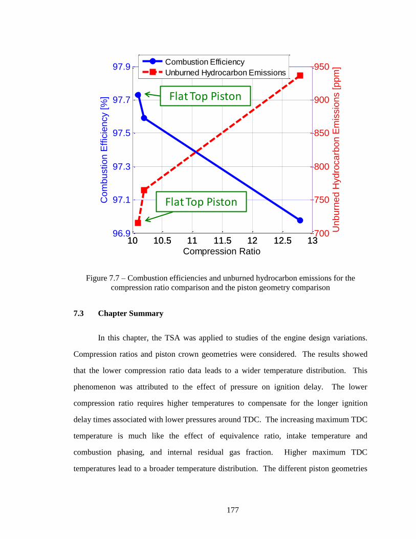
177

Figure 7.7 – Combustion efficiencies and unburned hydrocarbon emissions for the

compression ratio comparison and the piston geometry comparison

7.3 Chapter Summary

In this chapter, the TSA was applied to studies of the engine design variations.

Compression ratios and piston crown geometries were considered. The results showed

that the lower compression ratio data leads to a wider temperature distribution. This

phenomenon was attributed to the effect of pressure on ignition delay. The lower

compression ratio requires higher temperatures to compensate for the longer ignition

delay times associated with lower pressures around TDC. The increasing maximum TDC

temperature is much like the effect of equivalence ratio, intake temperature and

combustion phasing, and internal residual gas fraction. Higher maximum TDC

temperatures lead to a broader temperature distribution. The different piston geometries

10 10.5 11 11.5 12 12.5 1396.9

97.1

97.3

97.5

97.7

97.9

Co

mb

ustio

n E

ffic

ien

cy [

%]

Compression Ratio

10 10.5 11 11.5 12 12.5 13700

750

800

850

900

950

Un

bu

rne

d H

yd

roca

rbo

n E

mis

sio

ns [p

pm

]

Combustion Efficiency

Unburned Hydrocarbon Emissions

Flat Top Piston

Flat Top Piston

178

(e.g. flat piston top vs. a complex shape with an asymmetric piston bowl) produced a

surprisingly small impact on the naturally occurring thermal stratification.

179

CHAPTER 8

EFFECT OF A GLOW PLUG ON HCCI COMBUSTION

The previous chapters explored the effects of varying operating conditions on the

naturally occurring in-cylinder thermal stratification. These variables included

combustion phasing, fuel preparation, intake temperature, fueling rate, residual gas

fraction, wall temperature and material, compression ratio, and piston geometry. The

results showed some interesting and unexpected trends. First, the variables that affect

ignition delay, like mixture composition and pressure at ignition, will affect the

temperature distribution at a constant combustion phasing by changing the required

maximum TDC temperature. Additionally, combustion phasing alone spreads the

temperature distribution where the earlier phased operating conditions have a broader

distribution. Wall temperature and material were shown to have an effect. However, the

effect was much more subtle than expected with large changes in wall temperature or

material only having a small influence on the width of the distribution. Geometry did not

significantly alter the temperature distribution. Decreasing the compression ratio was

able to broaden the distribution due to the pressure effect on ignition delay. The lower

compression ratios require a higher maximum TDC temperature, spreading the

distribution.

Through these extensive studies of engine operating conditions and design

parameters, the effect of varying these conditions on the naturally occurring in-cylinder

temperature distribution through normal engine operation was better understood. This

chapter explores a more deliberate strategy to control the temperature distribution. The

idea is to use a glow plug (GP), normally used to help cold-start emissions in diesel

180

engines [109, 110], in HCCI, and by varying the glow plug voltage and temperature, the

in-cylinder temperature distribution may be influenced by a varying extent. Hopefully,

only the charge near the glow plug will be affected by the presence of the glow plug,

while the charge in other parts of the chamber will not. In which case, the glow plug

temperature could be used to spread the temperature distribution. This chapter explores

the effects of a glow plug on the unburned temperature distribution, and HCCI in general,

because there is no mention in the literature of using a glow plug in HCCI. Researchers

at Lund used a glow plug in PCCI and briefly mentioned that the operating condition was

more robust with the glow plug on [111]. Researchers at the University of Michigan and

elsewhere have explored the effects of spark plugs in HCCI and termed the combustion

mode SACI, for spark assisted compression ignition [30, 32-34]. But a glow plug has

never been used in HCCI and the effects were unknown until this dissertation.

8.1 Design, Construction, and Glow Plug Tip Temperature

A Beru pressure sensing glow plug was used in this experiment [112]. The

pressure sensing capabilities were not utilized. Only the electrical resistive heating

feature of the glow plug was used. Being a gasoline SI engine by nature, the engine

would not accept the Beru glow plug as is. Sleeve adapters needed to be designed and

constructed to allow the tip of the glow plug access to the combustion chamber. Two

different configurations were tested; a side mounted glow plug and a centrally mounted

glow plug.

8.1.1 Side Mounted Configuration

The first configuration that was tested involved constructing a sleeve adapter that

allowed the glow plug to be located in the heat flux probe port over the bowl. This way,

the spark plug can still be used to help start the engine. However, the side mount

181

configuration does require sacrificing one of the heat flux probes for the glow plug.

Also, the clearance between the head and the piston at this side position is very small

(about 0.2 inches). There was concern that this would not be enough penetration into the

chamber to see a noticeable effect. To solve the lack of clearance and short glow plug

extension problem, the adapter was designed to leave a 0.2 inch well or pocket around the

glow plug, bringing the total relative penetration up to around 0.4 inches. In contrast, the

heat flux probes were designed to be perfectly flush with the surface of the head so that

the surface temperature measurements are as accurate as possible. Figure 8.1 shows the

glow plug and sleeve adapter first by themselves, then assembled, to show how the glow

plug mount in the adapter.

Figure 8.1 – Glow plug and side mount sleeve adapter

182

Figure 8.2 shows the side mounted adapter sleeve and glow plug mounted in the

head of the engine. The intentional well around the glow plug is evident from the Figure

8.2 and it was important to ensure suitable penetration of the glow plug tip into the

chamber. The well does decrease the nominal compression ratio from 12.8:1 to 12.6:1.

The side glow plug configuration could also potentially be better for swirl studies since

the swirl control valve closes the intake port to the valve further from the glow plug in

Figure 8.2 meaning all of the intake charge would go through the valve closer to the glow

plug. A swirl study with the side mounted glow plug was not performed in this

dissertation and is a recommendation for future work.

Figure 8.2 – Glow plug and side mounted sleeve adapter installed in the head

183

8.1.2 Centrally Mounted Configuration

In addition to the side mounted configuration, a centrally mounted glow plug

configuration was tested. In this case, the glow plug replaces the spark plug. Both heat

flux probes can still be used but the spark plug is removed. The sleeve adapter in this

case is designed to have the same outer geometry as the spark plug but the inner

geometry allows the glow plug to mount in the sleeve and the tip to penetrate into the

combustion chamber. Because there is more clearance between the head and the piston

in the center of the chamber, the penetration for the centrally mounted glow plug is

around 0.5 inches and the compression ratio does not need to be reduced. Without the

spark plug, it can be very difficult to start the engine, especially when using a large

amount of internal residuals, because ignition depends on the presence of the hot

residuals and without the spark event there is nothing to trigger combustion initially.

Therefore, the centrally mounted glow plug will only be tested with the PVO camshafts

where starting without the spark plug is much easier. Figure 8.3 shows the centrally

mounted sleeve adapter with the glow plug installed.

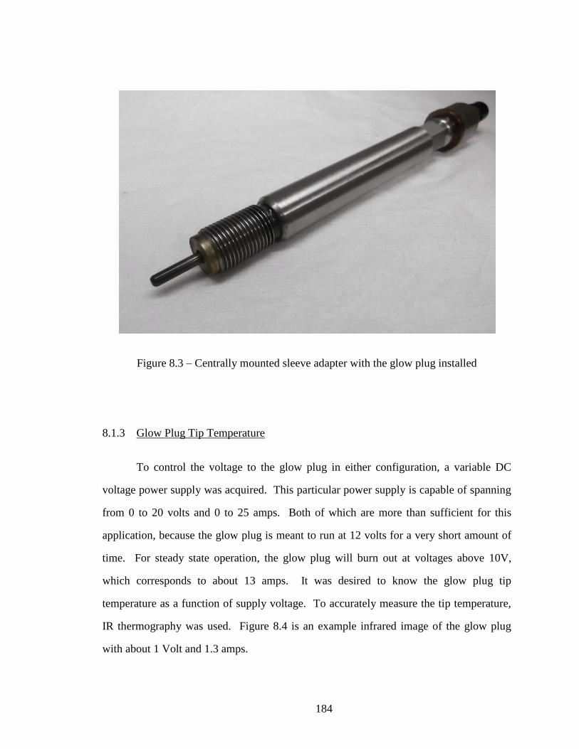
184

Figure 8.3 – Centrally mounted sleeve adapter with the glow plug installed

8.1.3 Glow Plug Tip Temperature

To control the voltage to the glow plug in either configuration, a variable DC

voltage power supply was acquired. This particular power supply is capable of spanning

from 0 to 20 volts and 0 to 25 amps. Both of which are more than sufficient for this

application, because the glow plug is meant to run at 12 volts for a very short amount of

time. For steady state operation, the glow plug will burn out at voltages above 10V,

which corresponds to about 13 amps. It was desired to know the glow plug tip

temperature as a function of supply voltage. To accurately measure the tip temperature,

IR thermography was used. Figure 8.4 is an example infrared image of the glow plug

with about 1 Volt and 1.3 amps.

185

Figure 8.4 – Example IR image of the glow plug to demonstrate how the temperature as a

function of voltage was determined

The infrared camera and software were calibrated at room temperature to

minimize the error in the guessed emissivity of the material. Figure 8.5 shows the glow

plug tip temperature as a function of voltage. The blue data points were calculated from

the infrared camera and images. The 1 Volt data point in Figure 8.5 is shown as an

example in Figure 8.4. These measurements were the most accurate way of measuring

the tip temperature. Attempts were made to measure the tip temperature with a standard

K-type thermocouple but the measured values were much lower than real temperatures

and it was suspected that the contact resistance between the thermocouple and glow plug

tip was too high and the thermocouple was acting as a heat sink and influencing the

measurement. Due to the difficulties in measuring the glow plug tip temperature through

any other means, the infrared camera was used. It is still not necessarily representative of

the glow plug tip temperatures when the glow plug is installed in the engine because the

186

thermal environment would be different. These measurements were taken in ambient

room conditions. When the glow plug is subject to the turbulence, elevated temperatures,

and differing heat loss pathways of the engine environment, the temperature will

certainly be different from these measurements. The measurements shown in Figure 8.5

are only meant to serve as estimations of the glow plug tip temperature as a function of

supply voltage.

The infrared measurements are limited to temperatures below 650 °C because this

camera and lens saturate around that temperature. As the voltage and temperature

increase, the glow plug begins to glow, and emit light in the visible range. At these

voltages, the temperature can be estimated by visual approximation based on the color of

the metal. This method lacks any real accuracy and again is only meant to serve as a

rough approximation for the glow plug tip temperature.

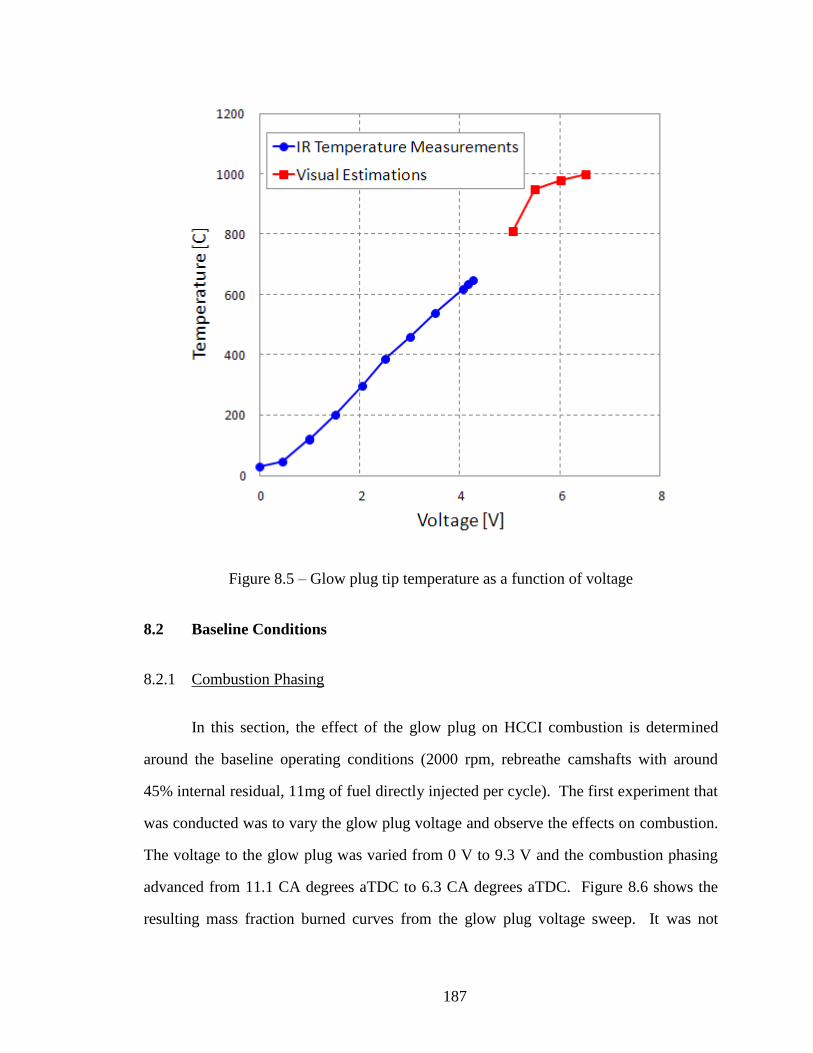
187

Figure 8.5 – Glow plug tip temperature as a function of voltage

8.2 Baseline Conditions

8.2.1 Combustion Phasing

In this section, the effect of the glow plug on HCCI combustion is determined

around the baseline operating conditions (2000 rpm, rebreathe camshafts with around

45% internal residual, 11mg of fuel directly injected per cycle). The first experiment that

was conducted was to vary the glow plug voltage and observe the effects on combustion.

The voltage to the glow plug was varied from 0 V to 9.3 V and the combustion phasing

advanced from 11.1 CA degrees aTDC to 6.3 CA degrees aTDC. Figure 8.6 shows the

resulting mass fraction burned curves from the glow plug voltage sweep. It was not

188

surprising that combustion phasing advanced by increasing the glow plug voltage

because the glow is in the end, just a resistive heating element. It is essentially acting to

heat the charge in the same way as the resistive heating intake heaters upstream in the

intake system. This experiment and the results in Figure 8.6 show that a glow plug can

be used to control combustion phasing within certain limits, since there are practical

limits on the glow plug’s voltage (i.e. the glow plug cannot go below 0 V and increasing

the glow voltage above 10 V would have burnt out the glow plug).

Figure 8.6 – Mass fraction burned curve for a glow plug voltage sweep

8.2.2 Temperature Distributions and Thermal Width

To this point, it is not clear if the glow has the same effect on HCCI as the intake

heater, or if the heat is not equally distributed to the charge resulting in a wider

temperature distribution. An intake temperature sweep was collected with the same

-10 0 10 20 30 40

0

0.2

0.4

0.6

0.8

1


Ma

ss F

ractio

n B

urn

ed

GP = 0V

GP = 6.5V

GP = 7.3V

GP = 8.2V

GP = 9.3V

189

conditions as the data in Figure 8.6 to help answer this question. For this sweep, the glow

plug was left off and the intake temperature was increased to advance combustion

phasing. Five data points were taken, matching the CA50 to each of the data points

shown in Figure 8.6. The intake temperature sweep is shown in Figure 8.7 with the glow

plug voltage sweep from Figure 8.6. The black “Tint = 100C, GP = 0V” curve serves as

the baseline data point and starting point for each of the sweeps. As the glow plug

voltage increased to 6.5V and the intake temperature increased 6 °C, the two data points

(solid and dashed blue lines) are very similar and it is difficult to see any differences

between the burn characteristics. However, as the voltage and intake temperature

continue to increase, the differences between the two methods for achieving the same

CA50 become evident. The glow plug data has a longer burn duration than the intake

temperature points, with the most noticeable difference in burn duration occurring at the

highest voltage and intake temperature, and earliest phasing, operating condition. The

longer burn duration can only be attributed to the presence of the glow plug and its

elevated temperature being that the glow plug and intake temperature are the only

differences between the two (magenta) data points. The addition of the intake

temperature sweep shows that, at these conditions, 9.3 Volts of glow plug power is worth

about 25 °C of intake temperature heating in terms of combustion phasing.

190

Figure 8.7 – Mass fraction burned curves for a glow plug voltage sweep and an intake

temperature sweep

The Thermal Stratification Analysis was used to process the nine operating

conditions in Figure 8.7 to determine the effect of the glow plug on the unburned

temperature distribution at TDC. The resulting distributions are shown in Figure 8.8.

The figure is a little crowded by the number of distributions. Later, the two earliest

phased cases will be plotted in their own figure so that the differences can be better

understood. The goal of Figure 8.8 is to show that both sweeps exhibit a strong effect of

combustion phasing and increasing intake temperature that was previously observed. The

near-wall regions of all nine operating conditions come together. The differences in the

temperature distributions for the second latest (blue) CA50 pair and the mid-phased (red)

CA50 pair is negligible. But as the glow plug voltage increases, the differences become

more significant.

-10 0 10 20 30 40

0

0.2

0.4

0.6

0.8

1


Ma

ss F

ractio

n B

urn

ed

Tint

= 100C,

GP = 0V

Tint

= 106C

Tint

= 112C

Tint

= 118C

Tint

= 125C

GP = 6.5V

GP = 7.3V

GP = 8.2V

GP = 9.3V

191

Figure 8.8 – Unburned temperature distributions at TDC for a glow plug voltage sweep

and an intake temperature sweep

Figure 8.9 shows the earliest and second earliest phased CA50 pairs from Figure

8.8. The effect of the glow plug on the unburned temperature distribution is much clearer

in Figure 8.9. The near-wall region is relatively unaffected. However, the hottest leading

edge of the distribution is greatly affected by the glow plug. With the glow plug on

(dashed lines), the temperature distribution is stretched towards higher temperatures. The

glow plug is able to heat some small percent of the mass to a much higher temperature.

As a result of the stretching of the leading edge of the distribution, the peak of the

distribution is lower and the thermal width is larger with the glow plug on. The glow

plug did have the desired effect of stretching the distribution and offers the potential to

control the width of the temperature distribution to some extent.

900 950 1000 1050 11000

0.002

0.004

0.006

0.008

0.01

0.012

0.014


Ma

ss P

DF

T

int = 100C,

GP = 0V

Tint

= 106C

Tint

= 112C

Tint

= 118C

Tint

= 125C

GP = 6.5V

GP = 7.3V

GP = 8.2V

GP = 9.3V

192

Figure 8.9 – Unburned temperature distributions for the earliest two phased CA50 pairs

for a glow plug voltage sweep and an intake temperature sweep

The 10% to 90% and the 25% to 75% thermal widths for the glow plug voltage

sweep and the intake temperature sweep are shown in Figure 8.10. As the glow plug

voltage increases and the combustion phasing advances, the difference between the

thermal width of the glow plug sweep and the intake temperature sweep increases. For

the highest glow plug voltage and earliest combustion phasing CA50 pair, the 10% to

90% and 25% to 75% thermal width with the glow plug on is 5.3% and 3.3% larger than

the same CA50 phasing achieved with intake temperature instead of the glow plug,

respectively. The 10% to 90% is more affected than the 25% to 75% because, by nature,

the glow plug is stretching the leading edge of the distribution and widening the

distribution by manipulating one of the tails.

900 950 1000 1050 1100 11500

0.002

0.004

0.006

0.008

0.01

0.012


Ma

ss P

DF

Tint

= 118C

Tint

= 125C

GP = 8.2V

GP = 9.3V

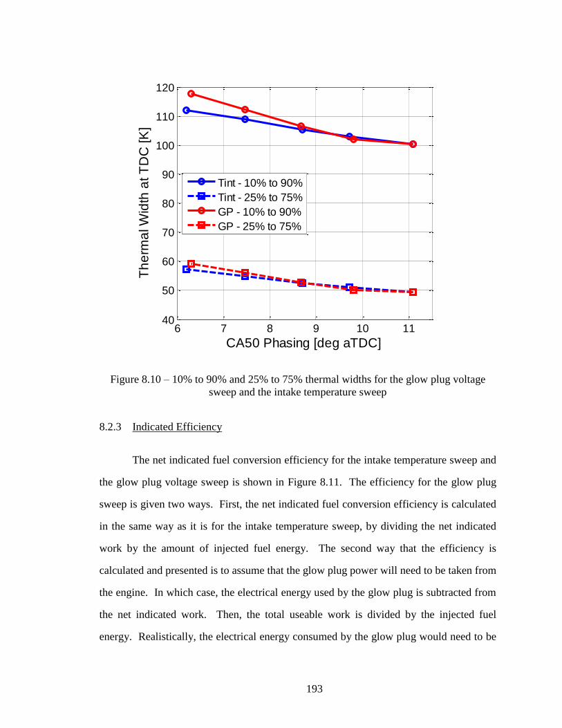
193

Figure 8.10 – 10% to 90% and 25% to 75% thermal widths for the glow plug voltage

sweep and the intake temperature sweep

8.2.3 Indicated Efficiency

The net indicated fuel conversion efficiency for the intake temperature sweep and

the glow plug voltage sweep is shown in Figure 8.11. The efficiency for the glow plug

sweep is given two ways. First, the net indicated fuel conversion efficiency is calculated

in the same way as it is for the intake temperature sweep, by dividing the net indicated

work by the amount of injected fuel energy. The second way that the efficiency is

calculated and presented is to assume that the glow plug power will need to be taken from

the engine. In which case, the electrical energy used by the glow plug is subtracted from

the net indicated work. Then, the total useable work is divided by the injected fuel

energy. Realistically, the electrical energy consumed by the glow plug would need to be

6 7 8 9 10 1140

50

60

70

80

90

100

110

120

CA50 Phasing [deg aTDC]

Th

erm

al W

idth

at T

DC

[K

]

Tint - 10% to 90%

Tint - 25% to 75%

GP - 10% to 90%

GP - 25% to 75%

194

produced by an alternator and there would be some efficiency associated with the

transformation from mechanical work to electrical energy. Rather than assume an

alternator efficiency, this transformation is neglected and the electrical energy is directly

subtracted from the net indicated work to get the useable mechanical work.

The net indicated fuel conversion efficiency for the intake temperature sweep

peaks somewhere around a CA50 phasing of 8.5 CA degrees aTDC. As the combustion

phasing gets later, the effective compression ratio is reduced, lowering the cycle’s

thermal efficiency. Also, the combustion efficiency decreases with later combustion

phasing. As combustion phasing advances, the heat transfer losses increase. When

excluding the power consumed by the glow plug, the glow plug voltage sweep also

shows a maximum, although it is at a little earlier combustion phasing than the maximum

of the intake temperature sweep. This could be due to experimental variability or it could

be due to the increasing combustion efficiency (discussed later) with glow plug voltage

and the lengthening burn duration. When the glow plug power is counted against the fuel

conversion efficiency, the difference between the efficiency calculated with and without

including the consumed glow plug energy increases with glow plug voltage. As a result,

the efficiency decreases with advancing combustion phasing. The total efficiency penalty

at the highest voltage setting (9.3 Volts) was 1.4 percentage points or 3.2%. This is a

noticeable, non-negligible amount. However, for the ability to control the temperature

distribution and burn duration, it is not so much that it would prohibit the use of a glow

plug in HCCI.

195

Figure 8.11 –Net indicated fuel conversion efficiency for the intake temperature sweep

and the glow plug voltage sweep

8.3 Lower Engine Speed Operation

8.3.1 Combustion Phasing and Temperature Distributions

In addition to understanding the effects of the glow plug on HCCI combustion

around the baseline operating conditions, it was hypothesized that the glow plug’s

influence may be enhanced at lower engine speeds because there is more time for the

glow plug to transfer heat to the charge at lower speeds. This section conducts the same

experiment as the previous section, except in this section the engine speed is decreased

from 2000 rpm to 1200 rpm. First, the glow plug voltage sweep and the intake

temperature sweep are shown in Figure 8.12. The results are very similar to the 2000

6 7 8 9 10 110.43

0.432

0.434

0.436

0.438

0.44

0.442

0.444

0.446

CA50 [deg aTDC]

Ne

t F

ue

l C

on

ve

rsio

n E

ffic

ien

cy

Intake Temperature Sweep

GP Sweep - excl. GP power

GP - incl. GP power

196

rpm experiment with the earliest phased, and highest glow plug voltage, point having a

longer burn duration than its CA50 pair.

Figure 8.12 – Mass fraction burned curves for the glow plug voltage sweep and the intake

temperature sweep at 1200 rpm

The glow plug voltage and intake temperature sweep comparisons are very useful

for understanding how the glow plug voltage can control combustion phasing within

certain limits. Also, these sweeps demonstrate that the glow plug is broadening the

temperature distribution and lengthening the burn duration at the higher glow plug

voltage points. However, these sweeps couple the glow plug voltage to advancing

combustion phasing. To help clarify the results, a third sweep was performed and

compared to the intake temperature sweep. In this third sweep, the glow plug voltage is

held constant at 7 Volts while the intake temperature is again used to vary the combustion

phasing matching CA50 to the previous sweeps. Figure 8.13 shows the mass fraction

-10 0 10 20 30 40

0

0.2

0.4

0.6

0.8

1


Ma

ss F

ractio

n B

urn

ed

Tint

= 138C,

GP = 0V

Tint

= 145C

Tint

= 154C

Tint

= 162C

Tint

= 167C

GP = 5V

GP = 6.5

GP = 8V

GP = 9.3V

197

burned curves for the two intake temperature sweeps; one with the glow plug off and one

with the glow plug on at 7 Volts (dashed lines labeled “GP” in the legend). With the

constant glow plug voltage, the effect on the burn durations now appears constant with

combustion phasing. The burn durations for the later phased operating conditions are

lengthened as well as the earlier phased operating conditions. At 1200 rpm, 7 Volts from

the glow plug is worth around 20 °C of intake temperature heating in terms of CA50

phasing.

Figure 8.13 – Mass fraction burned curves for the constant glow plug voltage intake

temperature sweep and the intake temperature sweep without the glow plug at 1200 rpm

At each CA50 phasing other than the latest, there are three different glow plug

voltages. The latest phasing condition only has two glow plug voltages. Figure 8.14

shows the three different glow plug voltage settings at the second latest condition. The

effect of the glow plug on the distribution is the same as what was previously observed at

-10 0 10 20 30 40

0

0.2

0.4

0.6

0.8

1


Ma

ss F

ractio

n B

urn

ed

Tint

= 138C

Tint

= 145C

Tint

= 154C

Tint

= 162C

Tint

= 167C

GP, Tint

= 113C

GP, Tint

= 123C

GP, Tint

= 134C

GP, Tint

= 143C

GP, Tint

= 149C

198

2000 rpm. With the glow plug on, the leading edge is stretched toward higher

temperatures lowering the peak of the distribution. The 7 V case has a stronger effect

than the 5 V case, suggesting that the effect of the glow plug on the temperature

distribution increases with the glow plug voltage.

Figure 8.14 – Unburned temperature distributions for the three glow plug voltage settings

for the second latest phasing condition at 1200 rpm

Figure 8.15 shows the three glow plug voltage settings for the earliest phased

condition. The trends are the same as in Figure 8.14. The hottest leading edge of the

distribution is affected by the glow plug’s energy. As a result, the peak of the distribution

is lower and the distribution in general is broader. The glow plug’s effect on the

temperature distribution increases with the glow plug voltage. In this case, the 7 Volt

condition is almost perfectly located between the 0 Volt condition and the 9.3 Volt

condition.

960 980 1000 1020 1040 10600

0.002

0.004

0.006

0.008

0.01

0.012

0.014


Ma

ss P

DF

GP = 0V, Tint

= 145C

GP = 7V, Tint

= 123C

GP = 5V, Tint

= 138C

199

Figure 8.15 – Unburned temperature distributions for the three glow plug voltage settings

for the earliest phasing condition at 1200 rpm

Figure 8.16 shows the 10% to 90% thermal widths for the two intake temperature

sweeps, with and without the glow plug, and the glow plug voltage sweep. Note that the

25% to 75% thermal widths are not shown for clarity and simplicity. The 25% to 75%

thermal width shows the exact same trends that can be seen in the 10% to 90% thermal

width. The intake temperature sweep (solid black line) shows the same trend with intake

temperature and combustion phasing that has been shown several times. The glow plug

voltage sweep shows same trend that was seen in Figure 8.10. As the glow plug voltage

increases, the difference in thermal width increases. The constant (7 Volt) glow plug

voltage intake temperature sweep shows a relatively constant offset from the baseline

intake temperature sweep. In fact the glow plug voltage sweep crosses the constant glow

plug voltage intake temperature sweep around 7 volts. The maximum increase in thermal

960 980 1000 1020 1040 10600

0.002

0.004

0.006

0.008

0.01

0.012


Ma

ss P

DF

GP = 0V, Tint

= 167C

GP = 7V, Tint

= 149C

GP = 9.3V, Tint

= 138C

200

width caused by the glow plug is 4.3%. The effect of the glow plug at 1200 rpm is

approximately the same as the effect at 2000 rpm.

Figure 8.16 – 10% to 90% thermal widths for the intake temperature sweep, the constant

glow plug voltage intake temperature sweep, and the glow plug voltage sweep at 1200

rpm

8.3.2 Efficiency and Emissions

The net indicated fuel conversion efficiencies for the three sweeps are shown in

Figure 8.17. The trends at 1200 rpm are the same as the trends at 2000 rpm shown in

Figure 8.11. The increasing glow plug voltage means there is an increasing efficiency

penalty. At 1200 rpm, the efficiency penalty at 9.3 volts is 2.5 percentage points or 5.7%.

The efficiency penalty is much larger at 1200 rpm because the engine produces less

power, while the glow plug consumes the same amount.

6 7 8 9 1086

88

90

92

94

96

98

100

102

104

106

CA50 [deg aTDC]

Th

erm

al W

idth

at T

DC

[K

]

GP = 0V, Intake Temp Sweep


Tint

= 138C, GP Voltage Sweep

201

Figure 8.17 – Net indicated fuel conversion efficiency for the intake temperature sweep,

the constant glow plug voltage intake temperature sweep, and the glow plug voltage

sweep at 1200 rpm

The measured combustion efficiency for the glow plug operating conditions was

higher than the corresponding CA50 condition without the glow plug. The effect was

small but consistent. Figure 8.18 shows the combustion efficiency for the three sweeps at

1200 rpm. Combustion efficiency, in general, increases with combustion phasing. The

glow plug increases the combustion efficiency and the difference is proportional to the

glow plug voltage. The reason for the increased combustion efficiency is most likely due

to better hydrocarbon consumption from the elevated glow plug temperatures after

combustion.

5 6 7 8 9 10 110.4

0.405

0.41

0.415

0.42

0.425

0.43

0.435

0.44

CA50 [deg aTDC]

Ne

t F

ue

l C

on

ve

rsio

n E

ffic

ien

cy

Intake Temp Sweep

Constant GP Volts - excl. GP power

Constant GP Volts - incl. GP power

GP Voltage Sweep - excl. GP power

GP Voltage Sweep - incl. GP power

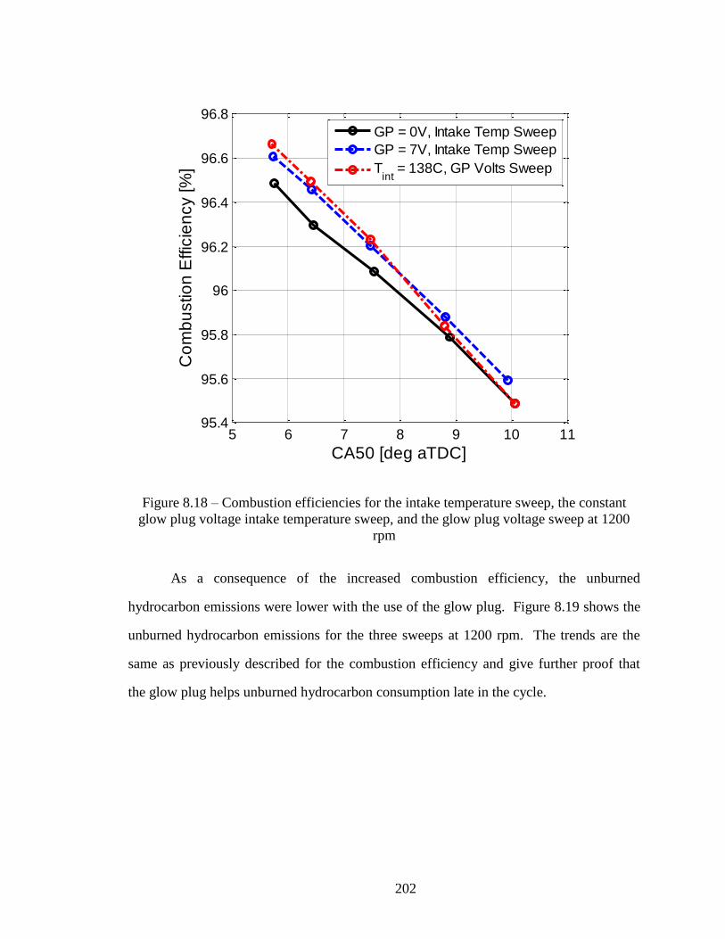
202

Figure 8.18 – Combustion efficiencies for the intake temperature sweep, the constant

glow plug voltage intake temperature sweep, and the glow plug voltage sweep at 1200

rpm

As a consequence of the increased combustion efficiency, the unburned

hydrocarbon emissions were lower with the use of the glow plug. Figure 8.19 shows the

unburned hydrocarbon emissions for the three sweeps at 1200 rpm. The trends are the

same as previously described for the combustion efficiency and give further proof that

the glow plug helps unburned hydrocarbon consumption late in the cycle.

5 6 7 8 9 10 1195.4

95.6

95.8

96

96.2

96.4

96.6

96.8

CA50 [deg aTDC]

Co

mb

ustio

n E

ffic

ien

cy [%

]



Tint

= 138C, GP Volts Sweep

203

Figure 8.19 – Unburned hydrocarbon emissions for the intake temperature sweep, the

constant glow plug voltage intake temperature sweep, and the glow plug voltage sweep at

1200 rpm

In addition to improving the unburned hydrocarbon emissions, the NOx emissions

are also improved with the use of the glow plug. Figure 8.20 shows the NOx emissions

for the three sweeps at 1200 rpm. The NOx emissions are reduced by as much as 15% at

the highest voltage setting. The mechanism for reducing NOx emission is through

lengthening the burn duration. The longer burn duration leads to a lower peak

temperature and fewer NOx emissions.

5 6 7 8 9 10 111050

1100

1150

1200

1250

1300

1350

1400

1450

1500

CA50 [deg aTDC]

Un

bu

rne

d H

yd

roca

rbo

n E

mis

sio

ns [p

pm

]



Tint


204

Figure 8.20 – NOx emissions for the intake temperature sweep, the constant glow plug

voltage intake temperature sweep, and the glow plug voltage sweep at 1200 rpm

8.4 Centrally Mounted Glow Plug

All of the previous data was collected using the side glow plug. But a centrally

mounted configuration was tested as well. This section shows the results form testing

with the centrally mounted glow plug. The positive valve overlap camshafts were used

so that the engine could be started without the spark plug, which was replaced with the

glow plug in this experiment. Figure 8.21 shows a mid-phased condition (CA50 is 8.6

CA degrees aTDC) that is representative of the centrally mounted glow plug trends in

general. The effect of the glow plug when centrally mounted using the PVO camshafts is

5 6 7 8 9 10 1114

16

18

20

22

24

26

28

30

32

CA50 [deg aTDC]

NO

x [p

pm

]



Tint


205

generally the same as was previously seen with the side mounted glow plug and the

rebreathe camshafts. The broadening of the temperature distribution is larger in this case,

with the thermal width increasing 6.8% to 7.0% due to the glow plug. Note that a 7%

wider temperature distribution, in this case, results in a 27% longer burn duration. It’s

not surprising that the effect of the glow plug is stronger with the centrally mounted

configuration because the penetration of the glow plug tip is deeper into the chamber.

With the centrally mounted glow plug, the tip extends 0.5 inches into the combustion

chamber, whereas the side mounted configuration needed to manufacture a 0.2 inch deep

pocket around the glow plug tip so that there is a total of 0.4 inches of penetration. Also,

it is possible that the glow plug’s influence on the temperature distribution is enhanced

with PVO operation. The lack of internal residuals with the PVO camshafts leads to a

much more uniform temperature distribution around IVC, possibly allowing the glow

plug to have a more significant impact on the thermal width.

206

Figure 8.21 – Representative unburned temperature distributions for the centrally

mounted glow plug with the PVO camshafts

8.5 Glow Plug with Swirl

Lastly, the glow plug was tested with and without swirl to determine if adding an

organized in-cylinder charge motion would enhance or attenuate the effects of the glow

plug on the unburned temperature distribution. As is the case with swirl, the PVO

camshafts were used so that there are no re-inducted residual gases to inhibit the directed

intake charge motion. Two more operating conditions were added to Figure 8.21; a swirl

case with the glow plug off and a swirl case with the glow plug at the same voltage as the

point in Figure 8.21 (6.3 Volts). Figure 8.22 shows the four point comparison. Both with

and without swirl, adding the glow plug spreads the distribution. However, the

distribution is widest with the glow plug on and without swirl. That is to say that with

850 900 950 1000 1050 11000

0.002

0.004

0.006

0.008

0.01

0.012

0.014

0.016


Ma

ss P

DF

GP = 0V

GP = 6.3V

207

the glow plug off, adding swirl spreads the distribution. But, with the glow plug on,

adding swirl narrows the distribution. The operating condition with the glow plug on

without swirl has the longest leading edge of the distribution. The difference between the

swirl cases (with and without the glow plug) is fairly small. The thermal widths for the

two swirl cases are only 3% different, whereas, the difference between the two points

without swirl is 7%. It could be that the addition of swirl mixes out the effect of the glow

plug. In which case, the glow plug is mostly acting as an intake heater. Without the

enhanced intake charge motion, the glow plug is able to spread the distribution a more

significant amount because the glow plug’s heat is transferred to some of the charge but

not all, resulting in a broader distribution.

Figure 8.22 – Unburned temperature distributions for the glow plug with swirl

comparison

850 900 950 1000 1050 11000

0.002

0.004

0.006

0.008

0.01

0.012

0.014

0.016


Ma

ss P

DF

GP = 0V, No Swirl

GP = 0V, Swirl

GP = 6.3V, No Swirl

GP = 6.3V, Swirl

208

Observations of the Coefficient of Variation

While the effect of the glow plug on the unburned temperature distribution is

intentional and desired and presents a way for the HCCI combustion engineers to control

the burn rates and potentially expand the operating range of HCCI, the glow plug is not

without its faults. The efficiency penalty was discussed and that is one drawback to using

the glow plug in HCCI. Another negative attribute of using the glow plug in HCCI is that

the glow plug caused the coefficient of variation to increase. The increase was small with

the rebreathe camshafts, but fairly considerable for the PVO camshafts. There are two

potential explanations for the increase in COV. First, it is possible that the glow plug’s

effect on the charge is not consistent from one cycle to the next, especially considering

the random turbulent motion during the intake stroke and how that could impact the heat

transfer from the glow plug to the charge. A second explanation as to why the COV

increases with the use of the glow plug is that the hot surface of the glow plug could be

producing flames. The timing of those flames is not controlled in any way and would

result in a large increase in COV. The fact that the increase in COV was larger with the

PVO camshafts and the more air dilute mixture suggests that this is in fact the case. The

presence of internal residuals helps to prevent surface flames form starting at the glow

plug tip, and in the case that flames do start at the glow plug tip, with a higher residual

gas fraction the flame speeds will be lower and have a smaller impact on COV and

combustion. The voltage was limited to 6.3 volts for the PVO experiment because if the

voltage was increased beyond that limit, the COV became unacceptable and potentially

dangerous. The strong sensitivity of the COV increase with glow plug voltage, especially

with the PVO camshafts, is another indicator that there are flames emanating from the

glow plug at random times during the cycle. Under one set of conditions (the centrally

mounted glow plug with the PVO camshafts without swirl) the NOx emission increased

slightly, rather than decrease like they did for all other conditions with the glow plug.

209

The higher NOx emissions, especially when the burn duration is longer and the peak bulk

temperature is lower, strongly suggest that the glow plug is producing flames under these

conditions.

This fact may make the use of a glow plug in HCCI combustion seem unpractical.

However, if the flames are the sole reason for the increase in COV, the glow plug could

be used as a compliment to a spark plug. That is, SACI has been shown to be a viable

option for HCCI and can help combustion researchers control both the start of

combustion and the burn rate [30, 32-34]. But SACI is only effective for mixtures that

can support flames and where the flame speed is not so low that the flame cannot travel

any relevant distance over the course of the combustion and expansion processes. Where

SACI is not effective, the glow plug could help to provide some control over the start and

rate of combustion.

8.6 Chapter Summary

In this chapter, an attempt was made to develop a method for active control of the

thermal stratification and resulting HCCI burn rates. A glow plug was installed in the

HCCI combustion chamber. This involved the construction of custom sleeve adapters in

the cylinder head to allow the glow plug access to the combustion chamber. A variable

DC voltage power supply was used to control the voltage and to observe its effects on

HCCI combustion. The effects of the glow plug were tested under different operating

conditions, such as the baseline operating conditions, a lower engine speed condition, and

when operating with the PVO camshaft with and without swirl. Both side mounted and

centrally mounted glow plug configurations were tested.

The results showed that the glow plug was able to control combustion phasing

within a certain range. More importantly, the glow plug was able to broaden the

temperature distribution and lengthen the burn duration a considerable amount. The

210

magnitude of the effect on the temperature distribution increased with glow plug voltage

and the centrally mounted glow plug with the PVO camshaft was more effective than the

side mounted glow plug. The glow plug was able to slightly improve some of the

emissions characteristics of HCCI and the combustion efficiency. The main drawbacks

of using a glow plug in HCCI are that there is an efficiency penalty associated with the

energy consumed by the glow plug and that the glow plug caused the COV to increase,

possibly due to flames originating from the hot glow plug tip.

211

CHAPTER 9

CONCLUSIONS, SCIENTIFIC CONTRIBUTIONS, AND

RECOMMENDATIONS FOR FUTURE WORK

9.1 Summary and Conclusions

HCCI is a promising advanced engine concept with the potential to pair high

thermal efficiencies with ultra-low emissions. HCCI has proven these capabilities only

over a narrow speed and load range. The limited range of operability stems from a lack

of control over HCCI burn rates and a general lack of understanding of the energy release

process in HCCI. The objective of this research was to further the understanding of the

HCCI energy release process by providing insight into the variables that affect the

unburned temperature distribution. To do this, a novel post-processing technique was

developed for studying thermal stratification in a fired metal HCCI engine. The

technique is called the Thermal Stratification Analysis (TSA) and it uses the autoignition

integral, with the assumption that the mass in the cylinder follows a self-similar

temperature contour, to predict ignition phasing of different temperature profiles. The

unburned charge temperature profiles are calculated based on the thermodynamic

relations for isentropic compression. Then, by comparing the ignition phasing of the

different temperature profiles to the mass fraction burned data and assuming that the

staggering of ignition phasing due to temperature stratification is the rate limiting factor

in the global combustion event, rather than the chemical reaction rates, a distribution of

mass and temperature in the cylinder prior to combustion is determined.

212

The capability of the TSA techniques has been assessed over a range of operating

conditions, and the observations were used for further refinement. The behavior near the

wall was non-physical because the TSA assumptions are no longer valid for the coldest

mass to burn. Therefore, the fraction of mass with non-physical behavior was discarded

from the distribution and the mass near the wall was included on the end of the

distribution by an exponential fit. This was driven by physical reasoning based on the

CARS measurements by Lucht [89] and the “Law of the Wall” from fluid mechanics.

With the unburned mass fit with an exponential function to the cold side of the

distribution, the complete distribution of mass and temperature is determined.

The TSA technique was then validated in two ways. First, output data from CFD

simulations was processed with the TSA, as if it were experimental data, and the resulting

unburned temperature distributions were compared to the known CFD temperature

distributions. The CFD validation showed that the absolute temperature range is

accurate, with the TSA-determined distributions spanning the same exact range of

temperatures as the CFD distributions. The peaks of the distributions were almost

perfectly co-located. The shapes were very similar as well, although the TSA-determined

distributions exhibited a much smoother leading edge and the CFD distributions

contained more information about the crevice volumes near the wall. It was found that

the TSA is most accurate for early and mid-phased operating conditions where the burn

rate is fast enough to not invalidate the No Mixing assumption.

Second, the TSA-determined distributions were compared to unburned

temperature distributions measured in an optical engine. It was found that the shapes

were extremely similar. The leading edge was always in great agreement. In general, the

optically measured distributions were narrower than the TSA-determined distributions

which could be attributed to the absence of the crevice mass in the optically measured

distributions. Also, it was determined that the TSA is only accurate around the phasing

of the combustion event and around TDC, and its accuracy diminishes when applied too

213

early in the compression stroke, or late in the expansion stroke. This was attributed to the

fact that the TSA generates a temperature distribution that is representative of the

particular combustion event, while the real in-cylinder distribution changes and evolves

over the course of the cycle due to turbulent charge motion and heat transfer effects.

Part II of this dissertation applies the TSA technique to analyze experimental data

obtained in a metal engine. A large amount of data was collected under varying

operating conditions to determine their effects on the in-cylinder unburned temperature

distribution, and explain the HCCI burn rate trends. This work produced the following

findings:

The differences between direct injection and fully premixing the fuel in

the intake stream were small

An injection timing sweep determined the injection timing limit, after

which compositional inhomogeneities exist around TDC

The presence of internal residuals and the valve strategy had a significant

impact on the unburned temperature distribution, where rebreathe

operation with a high internal residual gas fraction resulted in a much

wider temperature distribution than positive valve overlap with a low

internal residual gas fraction

Increasing intake temperature broadens the distribution by increasing the

maximum TDC temperature while leaving the wall region unaffected

Combustion phasing itself impacts the thermal width, where earlier

combustion phasing leads to a broader distribution, possibly due to the

increasing turbulent charge motion as TDC is approached

Adding swirl broadens the temperature distribution and the spread of the

distribution is slightly larger at earlier combustion phasing

Increasing the equivalence ratio while keeping combustion phasing

constant causes the distribution to narrow because the higher equivalence

214

ratio conditions have shorter ignition delays and require lower maximum

TDC temperatures

Next, efforts were made to understand the impact of wall conditions on the

unburned temperature distribution. The results showed a surprising insensitivity to wall

temperature and surface material. Higher wall temperatures did result in higher

combustion efficiencies and slightly less mass near the wall in the temperature

distribution. However, the impact on the temperature distribution for large changes in

wall temperature or material was very subtle. It was speculated that the insensitivity to

wall conditions is due to the exponential functional shape near the wall.

The next segment of the investigation applied the TSA to studies of the engine

design variations. Compression ratios and piston crown geometries were considered.

The results showed that a lower compression ratio leads to a wider temperature

distribution. This phenomenon was attributed to the effect of pressure on ignition delay.

The lower compression ratio requires higher temperatures to compensate for the longer

ignition delay times associated with lower pressures around TDC. The increasing

maximum TDC temperature is much like the effect of equivalence ratio, intake

temperature and combustion phasing, and internal residual gas fraction. Higher

maximum TDC temperatures lead to a broader temperature distribution. The different

piston geometries (e.g. flat piston top vs. a complex shape with an asymmetric piston

bowl) produced a surprisingly small impact on the naturally occurring thermal

stratification.

Finally, an attempt was made to develop a method for active control of the

thermal stratification and resulting HCCI burn rates. A glow plug was installed in the

HCCI combustion chamber. This involved the construction of custom sleeve adapters in

the cylinder head to allow the glow plug access to the combustion chamber. A variable

DC voltage power supply was used to control the voltage and to observe its effects on

HCCI combustion. The effects of the glow plug were tested under different operating

215

conditions, such as the baseline operating conditions, a low engine speed condition, and

when operating with the PVO camshaft with and without swirl. Both side mounted and

centrally mounted glow plug configurations were tested.

The results showed that the glow plug was able to control combustion phasing

within a certain range. More importantly, the glow plug was able to broaden the

temperature distribution and lengthen the burn duration a considerable amount. The

magnitude of the effect on the temperature distribution increased with glow plug voltage.

The centrally mounted glow plug with the PVO camshaft was more effective than the

side mounted glow plug. The glow plug was able to slightly improve some of the

emissions characteristics of HCCI and the combustion efficiency. The main drawbacks

of using a glow plug in HCCI are that there is an efficiency penalty associated with the

energy consumed by the glow plug and that the glow plug caused the COV to increase,

possibly due to flames originating from the hot glow plug tip.

9.2 Scientific Contributions

The major scientific contribution of this dissertation is the development and

validation of a post-processing methodology specific to HCCI operation that calculates

an unburned temperature distribution from the measured cylinder pressure. The

methodology is called Thermal Stratification Analysis. This post-processing technique is

relatively simple to implement and very inexpensive computationally. Therefore, it is

suitable for rapid assessment of the impact of design changes or variations of operating

conditions on the thermal stratification, and its correlation with HCCI burn rates. The

capabilities of the TSA, and the fact that it requires only crank-angle resolved pressure

traces rather than optical diagnostics, allows application to practical, metal engines, and

systematic investigations across a wide range of conditions. Prior to this work, the only

options were experiments on optical engines or CFD calculations, both capable of

216

generating deep insights, but very expensive and not suitable for engineering analyses

supporting development of a practical HCCI engine design or control.

Other significant contributions include the efforts to understand which variables

affect the unburned temperature distribution and HCCI burn rates. The results from

processing the experimental data with the traditional heat release analysis standalone as a

contribution of this work. A separate contribution is the results from processing the

collected experimental data with the Thermal Stratification Analysis. The uniqueness of

findings stems from the fact that the TSA technique is simultaneously qualitative and

quantitative. A wide range of operating conditions was studied and their impact

characterized, such as fuel preparation (direct injection vs. fully premixed charge, and

dilution with internal residual vs. air), intake temperature, positive valve overlap vs.

rebreathing, swirl, and wall temperature. The effect of the design changes, such as the

variation of the compression ratio or the piston top shape was investigated next. Last but

not least, knowledge generated through the systematic investigation mentioned above led

to development of an innovative method for active control of the thermal stratification

and HCCI burn rates. It is based on application of variable voltage glow-plugs, and the

method was proven to be effective over a reasonable range of conditions, with the only

drawbacks being the energy required to heat the glow plug and the increased cycle-to-

cycle variation. A summary of the original findings follows.

9.2.1 Characterization of the Impact of Design and Operating Conditions

While the effect of internal residuals on the temperature distribution has been

studied before [44, 46, and 49], and the broadening of the temperature distribution was

expected, the TSA allowed quantification of the expected trends in a fired metal engine.

The effects of ignition delay and mixture reactivity on the temperature

distribution in a practical application were unexpected at first, but intuitive in retrospect.

217

Decreasing the ignition delay of the mixture through compositional changes or pressure

at ignition results in a narrower temperature distribution at constant combustion phasing

because the maximum TDC temperature can decrease while the wall region stays

constant. In this way, temperature is not an independent variable under fired conditions.

The range of temperatures depends on the mixture composition and reactivity, and the

combustion phasing. The effect of ignition delay and changing maximum TDC

temperature was observed in the intake temperature sweep, the compensated load sweep,

combustion phasing study, residual gas fraction comparison, and the compression ratio

comparison.

Combustion phasing was found to affect the in-cylinder temperature distribution

with earlier phased conditions having a wider distribution. It was speculated that

increasing turbulence was responsible for broadening the distribution and a swirl study

was performed to test this hypothesis. It was found that adding swirl broadened the

temperature distribution and the effect was slightly stronger at earlier combustion

phasing.

Another contribution of this work was discovering the variables that somewhat

surprisingly did not impact the in-cylinder unburned temperature distribution. These

variables included wall temperature, piston surface material, and piston geometry. All of

these variables were expected to influence the unburned temperature distribution, but

contrarily were found to have only a very minor role in determining the naturally

occurring thermal stratification. That is not stay that these variables do not have any

impact on HCCI combustion. The effect during the open part of the cycle for the

changing wall temperature and material was significant (charge heating). However, the

effect on the temperature distribution and the HCCI burn rate was found to be small when

the phasing effect were compensated with intake temperature.

218

9.2.2 Control of Thermal Stratification with a Glow Plug

The final contribution of this work was to propose glow-plugs as means of

actively controlling thermal stratification and HCCI burn rates. All aspects of HCCI

were investigated, including combustion phasing, efficiency, and emissions, since a glow

plug has never been tested in an HCCI engine prior to this dissertation. The glow plug

stretched the distribution by non-uniformly heating the charge and increasing the

maximum TDC temperature while leaving most of the wall region unaffected. It was

shown that the glow plug enables control of the start and rate of HCCI combustion within

certain limits. The emissions characteristics were generally better with the glow plug, but

the efficiency penalty caused by the glow plug’s energy consumption needs to be

considered. The biggest drawback was the increased cycle-to-cycle variability associated

with the glow plug application.

9.3 Recommendations for Future Work

This work introduced a new post-processing technique for studying thermal

stratification in an HCCI engine. Then, as many engine operating conditions were

explored with the proposed technique as possible within the time constraints. The first

recommendation for future work is to continue the efforts based on TSA toward

understanding how additional operating conditions impact the in-cylinder temperature

distribution. This would include testing more compression ratios, additional engine

geometries, and different fuels to determine the effect on the unburned temperature

distribution. Changing the fuel properties is only possible if the effects on the ignition

delay correlation are known. That is to say that the activation energy would need to be

varied for each fuel or a different ignition delay correlation would need to be used. This

engine provided limited options when it comes to valve strategies. It was possible to use

only rebreathing and positive valve overlap operation, both with fixed valve profiles. It

219

would be interesting to know how variable negative valve overlap (NVO) impacts the

temperature distribution. With NVO, the residual gas fraction can be calculated with

more certainty, which may help understand the trends and increase confidence in the

absolute temperature range. Variable valve timing could be used to trap varying amounts

of internal residuals, and study the effect of varying compression ratio through either a

late or early intake valve closing strategy.

The effects of turbulence need further investigation, but must be done in an

optical engine to have concrete evidence and confidence in the results. The effects of

turbulence cannot be studied with certainty in a metal engine. In this research, swirl was

shown to spread the temperature distribution. In the future, the effects of other types of

intake charge motion could be studied (for example, tumble). With optical access, the

development of the in-cylinder temperature distribution with differing amounts of

turbulence could be studied to help shed light on the variables that affect the distribution

and how the distribution evolves over the intake and compression processes.

Lastly, this work demonstrated the potential of using a glow plug in an HCCI

engine. However, there is a lot more work that could be done to help understand the

physical phenomena. Optical data would help determine if there are flames and the

possible source of the increase in COV. The glow plug has a great potential to help make

HCCI much more controllable, but the increase in COV is a concern. The sources of

variability in HCCI were not a main focus of this work, but clearly need to be addressed

for the eventual success of HCCI. Additionally, different operating conditions could be

tested with the glow plug to understand if the observed effects are consistent or are

amplified or subdued in certain conditions. Higher powered glow plugs could be tested

with a larger surface area to help lengthen the burn duration and make HCCI more

controllable. In general, the glow plug results are extremely interesting and the glow

plug has the possibility to transform HCCI operation and control.

220

REFERENCES

[1] Onishi, S., Jo, S., Shoda, K., Jo, P., Kato, S. 1979, “Active Thermo Atmospheric

Combustion (ATAC) – A New Combustion Process for Internal Combustion

Engines,” SAE Paper 790501.

[2] Najt, P., Foster, D., 1983, “Compression-Ignited Homogeneous Charge

Combustion,” SAE Paper 830264.

[3] Thring, R., 1989, “Homogeneous Charge Compression Ignition (HCCI) Engines,”

SAE Paper 892068.

[4] Stanglmaier, R., Roberts, C., 1999, “Homogeneous Charge Compression Ignition

(HCCI): Benefits, Compromises, and Future Engine Applications,” SAE Paper

1999-01-3682.

[5] Epping, K., Aceves, S., Bechtold, R., Dec, J., 2002, “The Potential of HCCI

Combustion for High Efficiency and Low Emissions,” SAE Paper 2002-01-1923.

[6] Zhao, F., Asmus, T. N., Assanis, D. N., Dec, J. E., Eng, J. A., Najt, P. M.,

“Homogeneous Charge Compression Ignition (HCCI) Engines,” Warrendale:

Society of Automotive Engineers International, 2003.

[7] https://www-pls.llnl.gov/?url=science_and_technology-chemistry-combustion,

Combustion Chemistry, 2011.

221

[8] Lavoie, G. A., Heywood, J. B., and Keck, J. C., “Experimental and Theoretical

Investigation of Nitric Oxide Formation in Internal Combustion Engines,”

Combust. Sci. Technol., vol. 1, pp313-326, 1970.

[9] Heywood, J. B., “Internal Combustion Engine Fundamentals,” McGraw-Hill, Inc.,

1988.

[10] Dec, J., "A Conceptual Model of DI Diesel Combustion Based on Laser-Sheet

Imaging*," SAE Technical Paper 970873, 1997, doi:10.4271/970873.

[11] Wagner, U., Anca, R., Velji, A., and Spicher, U., "An Experimental Study of

Homogeneous Charge Compression Ignition (HCCI) with Various Compression

Ratios, Intake Air Temperatures and Fuels with Port and Direct Fuel Injection,"

SAE Technical Paper 2003-01-2293, 2003, doi:10.4271/2003-01-2293.

[12] Zigler, B. T., Keros, P. E., Helleberg, K. B., Fatouraie, M., Assanis, D.,

Wooldridge, M. S., “An Experimental Investigation of the Sensitivity of the

Ignition and Combustion Properties of a Single-Cylinder Research Engine to

Spark-Assisted HCCI,” International Journal of Engine Research 12 (2011) 353-

375.

[13] Zigler, B. T., Walton, S. M., Assanis, D., Perez, E., Wooldridge, M. S.,

Wooldridge, S. T., “An Imaging Study of Compression Ignition Phenomena of

Iso-Octane, Indolene, and Gasoline Fuels in a Single-Cylinder Research Engine,”

ASME Journal of Engineering for Gas Turbines and Power 130 (2008) 052803: 1-

11.

[14] Dec, J., Hwang, W., Sjoberg, M., “An Investigation of Thermal Stratification in

HCCI Engines Using Chemiluminescence Imaging,” SAE Paper 2006-01-1518.

222

[15] Richter, M., Engström, J., Franke, A., Aldén, M., Hultqvist, A., Johansson, B.,

2000, “The Influence of Charge Inhomogeneity on the HCCI Combustion

Process,” SAE Paper 2000-01-2868.

[16] Hultqvist A., Christensen, M., Johansson, B., Richter, M., Nygren, J. Hult, H.,

Aldén, M., 2002, “The HCCI Combustion Process in a Single Cycle – High-

Speed Fuel Tracer LIF and Chemiluminescence Imaging,” SAE Paper 2002-01-

0424.

[17] Sjöberg, M., Dec, J., and Cernansky, N., "Potential of Thermal Stratification and

Combustion Retard for Reducing Pressure-Rise Rates in HCCI Engines, Based on

Multi-Zone Modeling and Experiments," SAE Technical Paper 2005-01-0113,

2005, doi:10.4271/2005-01-0113.

[18] Sjöberg, M. and Dec, J., "Effects of Engine Speed, Fueling Rate, and Combustion

Phasing on the Thermal Stratification Required to Limit HCCI Knocking

Intensity," SAE Technical Paper 2005-01-2125, 2005, doi:10.4271/2005-01-2125.

[19] Yang, Y., Dec, J., Dronniou, N., Sjöberg, M. et al., "Partial Fuel Stratification to

Control HCCI Heat Release Rates: Fuel Composition and Other Factors Affecting

Pre-Ignition Reactions of Two-Stage Ignition Fuels," SAE Int. J. Engines

4(1):1903-1920, 2011, doi:10.4271/2011-01-1359.

[20] Milovanovic, N., Blundell, D., Pearson, R., Turner, J. et al., "Enlarging the

Operational Range of a Gasoline HCCI Engine By Controlling the Coolant

Temperature," SAE Technical Paper 2005-01-0157, 2005, doi:10.4271/2005-01-

0157.

223

[21] Park, D., Kim, H., and Kim, W., “A Study of Flame Propagation for Different

Combustion Chamber Configurations in an SI Engine," SAE Technical Paper

970876, 1997, doi:10.4271/970876.

[22] Siebers, D., "Liquid-Phase Fuel Penetration in Diesel Sprays," SAE Technical

Paper 980809, 1998, doi:10.4271/980809.

[23] Sjöberg, M. and Dec, J., "An Investigation of the Relationship Between Measured

Intake Temperature, BDC Temperature, and Combustion Phasing for Premixed

and DI HCCI Engines," SAE Technical Paper 2004-01-1900, 2004,

doi:10.4271/2004-01-1900.

[24] Hagen, L. M., Manofsky-Olesky, L., Bohac, S. V., Lavoie, G. and Assanis, D.,

“Effects of a Low Octane Gasoline Blended Fuel on Negative Valve Overlap

Enabled HCCI Load Limit, Combustion Phasing and Burn Duration,” J. Eng. Gas

Turbines Power 135(7), 2012.

[25] Hyvönen, J., Haraldsson, G., and Johansson, B., "Operating range in a Multi

Cylinder HCCI engine using Variable Compression Ratio," SAE Technical Paper

2003-01-1829, 2003, doi:10.4271/2003-01-1829.

[26] Hyvönen, J., Haraldsson, G., and Johansson, B., "Balancing Cylinder-to-Cylinder

Variations in a Multi-Cylinder VCR-HCCI Engine," SAE Technical Paper 2004-

01-1897, 2004, doi:10.4271/2004-01-1897.

[27] Maurya, R. and Agarwal, A., "Experimental Investigation of Close-Loop Control

of HCCI Engine Using Dual Fuel Approach," SAE Technical Paper 2013-01-

1675, 2013, doi:10.4271/2013-01-1675.

224

[28] Dec, J. and Sjöberg, M., "Isolating the Effects of Fuel Chemistry on Combustion

Phasing in an HCCI Engine and the Potential of Fuel Stratification for Ignition

Control," SAE Technical Paper 2004-01-0557, 2004, doi:10.4271/2004-01-0557.

[29] Popp, J. and Rutland, C., "Model-Based Feed-Forward Control of Diesel HCCI

Engine Transients," SAE Technical Paper 2009-01-1133, 2009, doi:10.4271/2009-

01-1133.

[30] Polovina, D., McKenna, D., Wheeler, J., Sterniak, J. et al., "Steady-State

Combustion Development of a Downsized Multi-Cylinder Engine with Range

Extended HCCI/SACI Capability," SAE Int. J. Engines 6(1):504-519, 2013,

doi:10.4271/2013-01-1655.

[31] Yang, Y., Dec, J., Dronniou, N., and Cannella, W., "Boosted HCCI Combustion

Using Low-Octane Gasoline with Fully Premixed and Partially Stratified

Charges," SAE Int. J. Engines 5(3):1075-1088, 2012, doi:10.4271/2012-01-1120.

[32] Manofsky, L., Vavra, J., Assanis, D., and Babajimopoulos, A., "Bridging the Gap

between HCCI and SI: Spark-Assisted Compression Ignition," SAE Technical

Paper 2011-01-1179, 2011, doi:10.4271/2011-01-1179.

[33] Persson, H., Sjöholm, J., Kristensson, E., Johansson, B. et al., "Study of Fuel

Stratification on Spark Assisted Compression Ignition (SACI) Combustion with

Ethanol Using High Speed Fuel PLIF," SAE Technical Paper 2008-01-2401,

2008, doi:10.4271/2008-01-2401.

[34] Szybist, J., Nafziger, E., and Weall, A., "Load Expansion of Stoichiometric HCCI

Using Spark Assist and Hydraulic Valve Actuation," SAE Int. J. Engines 3(2):244-

258, 2010, doi:10.4271/2010-01-2172.

225

[35] Lawler, B., Ortiz-Soto, E., Gupta, R., Peng, H. et al., "Hybrid Electric Vehicle

Powertrain and Control Strategy Optimization to Maximize the Synergy with a

Gasoline HCCI Engine," SAE Int. J. Engines 4(1):1115-1126, 2011,

doi:10.4271/2011-01-0888.

[36] Lawler, B. and Filipi, Z., “Integration of a Dual-Mode SI-HCCI Engine into

Various Vehicle Architectures,” Journal of Engineering for Gas Turbines and

Power, In Press

[37] Chang, J., Guralp, O., Filipi, Z., Assanis D., Kuo, T., Najt, P., Rask, R., “New

Heat Transfer Correlation for an HCCI Engine Derived from Measurements of

Instantaneous Surface Heat Flux,” SAE Paper 2004-01-2996.

[38] Chang, J., Filipi, Z., Assanis, D., Kuo, T., Najt, P., Rask, R., “Characterizing the

Thermal Sensitivity of a Gasoline Homogeneous Charge Compression Ignition

Engine with Measurements of Instantaneous Wall Temperature and Heat Flux,”

Int. J. of Engine Research, Vol. 6, No. 4, London, 2005, pp. 289-309.

[39] Guralp, O., Hoffman, M., Assanis, D., Filipi, Z., Kuo, T., Najt, P., Rask, R.,

“Characterizing the Effect of Combustion Chamber Deposits on a Gasoline HCCI

Engine,” SAE Paper 2006-01-3277.

[40] Guralp, O., Hoffman, M., Assanis, D., Filipi, Z., Kuo, T., Najt, P., Rask, R.,

“Thermal Characterization of Combustion Chamber Deposits on the HCCI

Engine Piston and Cylinder Head Using Instantaneous Temperature

Measurements,” SAE Paper 2009-01-0668.

[41] Chang J., Filipi Z., Assanis D., Kuo T., Najt P., and Rask R., “Investigation of

Mixture Preparation Effects on Gasoline HCCI Combustion Aided by

226

Measurements of Wall Heat Flux,” Proceedings of the ASME 2007 Internal

Combustion Engine Division Fall Technical Conference, ICEF2007-1698,

Charleston, South Carolina, USA, October 14–17, 2007.

[42] Kwon, O., Jeong, D., Lim, O., and Iida, N., "The Research about Thermal

Stratification Effect on Pressure Rise Rate in Supercharged HCCI Engine based

on Numerical Analysis," SAE Technical Paper 2009-32-0141, 2009.

[43] Dec, J., Hwang, W., “Characterizing the Development of Thermal Stratification in

an HCCI Engine Using Planar-Imaging Thermometry, SAE Paper 2009-01-0650.”

[44] Snyder, J., Dronniou, N., Dec, J., and Hanson, R., "PLIF Measurements of

Thermal Stratification in an HCCI Engine under Fired Operation," SAE Int. J.

Engines 4(1):1669-1688, 2011, doi:10.4271/2011-01-1291.

[45] Dronniou, N. and Dec, J., "Investigating the Development of Thermal

Stratification from the Near-Wall Regions to the Bulk-Gas in an HCCI Engine

with Planar Imaging Thermometry," SAE Int. J. Engines 5(3):1046-1074, 2012,

doi:10.4271/2012-01-1111.

[46] Rothamer, D., Snyder, J., Hanson, R., Steeper, R., Fitzgerald, R., “Simultaneous

imaging of exhaust gas residuals and temperature during HCCI combustion,”

Proceedings of the Combustion Institute 32 (2009) 2869-2876, 2009, doi:

10.1016/j.proci.2008.07.018.

[47] Kaiser, S., Schild, M., Schulz, C., “Thermal stratification in an internal

combustion engine due to wall heat transfer measured by laser-induced

fluorescence,” Proceedings of the Combustion Institute, In Press, 2012, doi:

10.1016/j.proci.2012.05.059.

227

[48] Woschni, G., "A Universally Applicable Equation for the Instantaneous Heat

Transfer Coefficient in the Internal Combustion Engine," SAE Technical Paper

670931, 1967, doi:10.4271/670931.

[49] Kodavasal, J., “Effect of Charge Preparation Strategy on HCCI Combustion,”

Ph.D. Thesis, University of Michigan, 2013.

[50] Andreatta, D.A., “The use of reformed natural gas as a fuel for reciprocating

engines,” Ph.D. dissertation, University of California at Berkeley, Dept. of

Mechanical Engineering, 1995.

[51] Noda, T., and Foster, D.E., “A Numerical Study to Control Combustion Duration

of Hydrogen-Fueled HCCI by Using Multi-Zone Chemical Kinetics Simulation,”

SAE Paper 2001-01-0250, 2001.

[52] Aceves, S.M., Martinez-Frias, J., Flowers, D.L., Smith, J.R., Dibble, R.W.,

Wright, J.F., and Hessel, R.P., “A Decoupled Model of Detailed Fluid Mechanics

Followed by Detailed Chemical Kinetics for Prediction of Iso-Octane HCCI

Combustion,” SAE Paper 2001-01-3612, 2001.

[53] Aceves, S.M., Flowers, D.L., Martinez-Frias, J., Smith, J.R., Westbrook, C.K.,

Pitz, W.J., Dibble, R.W., Wright, J.F., Akinyemi, W.C., and Hessel, R.P., “A

Sequential Fluid-Mechanic Chemical-Kinetic Model of Propane HCCI

Combustion,” SAE Paper 2001-01-1027, 2001.

[54] Babajimopoulos, A., Lavoie, G.A., and Assanis, D.N., “Modeling HCCI

combustion with high levels of residual gas fraction – a comparison of two VVA

strategies,” SAE Paper 2003-01-3220, 2003.

228

[55] Aceves, S., Flowers, D., Chen, J., and Babajimopoulos, A., "Fast Prediction of

HCCI Combustion with an Artificial Neural Network Linked to a Fluid

Mechanics Code," SAE Technical Paper 2006-01-3298, 2006, doi:10.4271/2006-

01-3298.

[56] Aceves, S., Flowers, D., Westbrook, C., Smith, J. et al., "A Multi-Zone Model for

Prediction of HCCI Combustion and Emissions," SAE Technical Paper 2000-01-

0327, 2000, doi:10.4271/2000-01-0327.

[57] Babajimopoulous, A., Assanis, D., Flowers, D., Aceves, S., Hessel, R., “A Fully

Coupled Computational Fluid Dynamics and Multi-zone Model with Detailed

Chemical Kinetics for the Simulation of Premixed Charge Compression Ignition

Engines,” Int. J. of Engine Research, Vol. 6, No. 5, pp. 497-512.

[58] Fiveland, S. and Assanis, D., "Development of a Two-Zone HCCI Combustion

Model Accounting for Boundary Layer Effects," SAE Technical Paper 2001-01-

1028, 2001, doi:10.4271/2001-01-1028.

[59] Flowers, D., Aceves, S., Martinez-Frias, J., Hessel, R. et al., "Effect of Mixing on

Hydrocarbon and Carbon Monoxide Emissions Prediction for Isooctane HCCI

Engine Combustion Using a Multi-zone Detailed Kinetics Solver," SAE Technical

Paper 2003-01-1821, 2003, doi:10.4271/2003-01-1821.

[60] Bedoya, I., Cadavid, F., Saxena, S., Dibble, R. et al., "A Sequential Chemical

Kinetics-CFD-Chemical Kinetics Methodology to Predict HCCI Combustion and

Main Emissions," SAE Technical Paper 2012-01-1119, 2012, doi:10.4271/2012-

01-1119.

229

[61] Mo, Y., “HCCI heat release rate and combustion efficiency: a coupled KIVA

multi-zone modeling study,” Doctor of Philosophy, University of Michigan, Ann

Arbor, 2008.

[62] Curran, H., Gafurri, P., Pitz, W.J., and Westbrook, C.K., “A Comprehensive

Modeling Study of iso-Octane Oxidation,” Combust & Flame 129:253-280, 2002.

[63] Aceves, S., Flowers, D., Westbrook, C., Smith, J. et al., "A Multi-Zone Model for

Prediction of HCCI Combustion and Emissions," SAE Technical Paper 2000-01-

0327, 2000, doi:10.4271/2000-01-0327.

[64] Aceves, S., Flowers, D., Martinez-Frias, J., Smith, J. et al., "A Sequential Fluid-

Mechanic Chemical-Kinetic Model of Propane HCCI Combustion," SAE

Technical Paper 2001-01-1027, 2001, doi:10.4271/2001-01-1027.

[65] Aceves, S., Flowers, D., Espinosa-Loza, F., Babajimopoulos, A. et al., "Analysis

of Premixed Charge Compression Ignition Combustion With a Sequential Fluid

Mechanics-Multizone Chemical Kinetics Model," SAE Technical Paper 2005-01-

0115, 2005, doi:10.4271/2005-01-0115.

[66] Babajimopoulos, A., Assanis, D.N., Flowers, D., Aceves, S., and Hessel, R., “A

fully coupled computational fluid dynamics and multi-zone model with detailed

chemical kinetics for the simulation of premixed charge compression ignition

engines,” International Journal of Engine Research, 6(5), pp. 497- 512, 2007.

[67] Livengood, J., Wu, P., Correlation of Autoignition Phenomena in Internal

Combustion Engines and Rapid Compression Machines, In Proceedings of the

Fifth International Symposium on Combustion, Pittsburgh, Pennsylvania, USA,

August 30th – September 3rd 1954, 1955, pp.347-356 (Reinhold, New York).

230

[68] Teraji, A., Tsuda, T., Noda, T., Kubo, M., Itoh, T., 2003, Development of a Three-

Dimensional Knocking Simulation for Spark Ignition Engines, SAE Paper 2003-

08-0360.

[69] Swan, K., Shahbakhti, M., Koch, C., 2006, Predicting Start of Combustion Using

a Modified Knock Integral Method for an HCCI Engine, SAE Paper 2006-01-

1086.

[70] Gatowski, J., Balles, E., Chun, K., Nelson, F. et al., "Heat Release Analysis of

Engine Pressure Data," SAE Technical Paper 841359, 1984, doi:10.4271/841359.

[71] Brunt, M., Rai, H., and Emtage, A., "The Calculation of Heat Release Energy

from Engine Cylinder Pressure Data," SAE Technical Paper 981052, 1998,

doi:10.4271/981052.

[72] Guezennec, Y. and Hamama, W., "Two-Zone Heat Release Analysis of

Combustion Data and Calibration of Heat Transfer Correlation in an I. C.

Engine," SAE Technical Paper 1999-01-0218, 1999, doi:10.4271/1999-01-0218.

[73] Catania, A., Misul, D., Mittica, A., and Spessa, E., "Unsteady Convection Model

for Heat Release Analysis of IC Engine Pressure Data," SAE Technical Paper

2000-01-1265, 2000, doi:10.4271/2000-01-1265.

[74] Kulzer, A., Lejsek, D., Kiefer, A., and Hettinger, A., "Pressure Trace Analysis

Methods to Analyze Combustion Features and Cyclic Variability of Different

Gasoline Combustion Concepts," SAE Technical Paper 2009-01-0501, 2009,

doi:10.4271/2009-01-0501.

[75] Fathi, M., Saray, R. K., and Checkel, M. D., “Detailed approach for apparent heat

release analysis in HCCI engines,” Fuel, vol. 89, no. 9, pp. 2323–2330, Sep. 2010.

231

[76] Stivender, D., "Development of a Fuel-Based Mass Emission Measurement

Procedure," SAE Technical Paper 710604, 1971, doi:10.4271/710604.

[77] Fitzgerald, R., Steeper, R., Snyder, J., Hanson, R. et al., "Determination of Cycle

Temperatures and Residual Gas Fraction for HCCI Negative Valve Overlap

Operation," SAE Int. J. Engines 3(1):124-141, 2010, doi:10.4271/2010-01-0343.

[78] Hohenberg, G., "Advanced Approaches for Heat Transfer Calculations," SAE

Technical Paper 790825, 1979, doi:10.4271/790825.

[79] Hensel, S., Sarikoc, F., Schumann, F., Kubach, H. et al., "A New Model to

Describe the Heat Transfer in HCCI Gasoline Engines," SAE Int. J. Engines

2(1):33-47, 2009, doi:10.4271/2009-01-0129.

[80] Annand, W. J. D., “Heat Transfer in the Cylinder of Reciprocating Internal

Combustion Engines”, Proc Instn Mech Engrs, Vol. 177, pp 973-990, 1963.

[81] “NIST-JANAF Thermochemical Tables.” http://kinetics.nist.gov/janaf/.

[82] He, X., Donovan, M., Zigler, B., Palmer, T., Walton, S., Wooldridge, M., Attreya,

A., 2005, An Experimental and Modeling Study of Iso-octane Ignition Delay

Times under Homogeneous Charge Compression Ignition Conditions,

Combustion and Flame 142 (2005): 266-275.

[83] Sjöberg, M. and Dec, J., "Smoothing HCCI Heat-Release Rates Using Partial Fuel

Stratification with Two-Stage Ignition Fuels," SAE Technical Paper 2006-01-

0629, 2006, doi:10.4271/2006-01-0629.

[84] Martz, J. B., Lavoie, G. A., Im, H. G., Middleton, R. J., Babajimopoulos, A.,

Assanis, D. N., “The propagation of a laminar reaction front during end-gas auto-

232

ignition,” Combustion and Flame, Volume 159, Issue 6, June 2012, Pages 2077-

2086, ISSN 0010-2180, http://dx.doi.org/10.1016/j.combustflame.2012.01.011.

[85] Martz, J.B., Middleton, R.J., Lavoie, G.A., Babajimopoulos, A., Assanis, D.N., “A

computational study and correlation of premixed isooctane–air laminar reaction

front properties under spark ignited and spark assisted compression ignition

engine conditions,” Combustion and Flame, Volume 158, Issue 6, June 2011,

Pages 1089-1096, ISSN 0010-2180, doi:10.1016/j.combustflame.2010.09.014.

[86] Middleton, R. J., Martz, J. B., Lavoie, G. A., Babajimopoulos, A., Assanis, D. N.,

“A computational study and correlation of premixed isooctane air laminar reaction

fronts diluted with EGR,” Combustion and Flame, Volume 159, Issue 10, October

2012, Pages 3146-3157, ISSN 0010-2180, doi:10.1016/2012.04.014.

[87] Martz, J.B. , Kwak, H., Im, H.G., Lavoie, G.A., Assanis, D.N., “Combustion

regime of a reacting front propagating into an auto-igniting mixture,” Proceedings

of the Combustion Institute, Volume 33, Issue 2, 2011, Pages 3001-3006, ISSN

1540-7489, http://dx.doi.org/10.1016/j.proci.2010.07.040.

[88] Lawler, B., Hoffman, M., Filipi, Z., Güralp, O., Najt, P., “Development of a post-

processing methodology for studying thermal stratification in an HCCI engine,” J.

Eng. Gas Turbines Power 134, 102801 (2012), 2012.

[89] Lucht, R., Dunn-Rankin, D., Walter, T., Dreier, T. et al., "Heat Transfer in

Engines: Comparison of Cars Thermal Boundary Layer Measurements and Heat

Flux Measurements†," SAE Technical Paper 910722, 1991, doi:10.4271/910722.

[90] Babajimopoulos, A., Lavoie, G. A., and Assanis, D. N., “On the Role of Top Dead

Center Conditions in the Combustion Phasing of Homogeneous Charge

233

Compression Ignition Engines,” Combustion Science and Technology, Vol. 179,

No. 9, 2039 – 2063, 2007.

[91] Gauthier, B.M., Davidson, D.F., and Hanson, R.K., “Shock tube determination of

ignition delay times in full-blend and surrogate fuel mixtures,” Combust. Flame,

139, 300–311, 2004.

[92] Davidson, D.F., Gauthier, B.M., and Hanson, R.K., “Shock tube ignition

measurements of iso-octane/air and toluene/ar at high pressures,” Proc. Combust.

Inst., 30, 1175–1182, 2005.

[93] Goldsborough, S.S., “A chemical kinetically based ignition delay correlation for

iso-octane covering a wide range of conditions including the NTC region,”

Combustion and Flame, Vol.156, pp.1248-1262, 2009.

[94] Private communication, Jeremie Dernotte, John Dec, Benjamin Lawler, Paul Najt,

and Zoran Filipi, November 7th

, 2011.

[95] Sjöberg, M., Dec, J., Babajimopoulos, A., and Assanis, D., "Comparing Enhanced

Natural Thermal Stratification Against Retarded Combustion Phasing for

Smoothing of HCCI Heat-Release Rates," SAE Technical Paper 2004-01-2994,

2004, doi:10.4271/2004-01-2994.

[96] Lacey, J., Sathasivam, S., Filipi, Z., Cannella, W., Fuentes-Afflick, P., “Impact of

refinery stream gasoline property variation on load sensitivity of the HCCI

combustion,” Proceedings of the ASME 2012 Internal Combustion Engine

Division Spring Technical Conference, ICES2012-81207, Torino, Piemonte, Italy,

May 6-9, 2012.

234

[97] Lacey, J., Sathasivam, S., Filipi, Z., Cannella, W., Fuentes-Afflick, P., “HCCI

operability limits: the impact of refinery stream gasoline property variation,”

Proceedings of the ASME 2012 Internal Combustion Engine Division Fall

Technical Conference, ICEF2012-92129, Vancouver, BC, Canada, September 23-

26, 2012.

[98] Lacey, J., “The Effects of Advanced Fuels and Additives on Homogeneous

Charge Compression Ignition Combustion and Deposit Formation,” Doctor of

Philosophy, University of Michigan, Ann Arbor, 2013.

[99] Fitzgerald, R., Steeper, R., and Snyder, J., "Effects of LIF Tracers on Combustion

in a DI HCCI Engine," SAE Int. J. Fuels Lubr. 1(1):1491-1502, 2009,

doi:10.4271/2008-01-2407.

[100] Güralp, O., “The Effect of Combustion Chamber Deposits on Heat Transfer and

Combustion in a Homogeneous Charge Compression Ignition Engine,” Ph.D.

Thesis, University of Michigan, 2008.

[101] Chang, K., “Modeling and Analysis of an HCCI Engine During Thermal

Transients Using a Thermodynamic Cycle Simulation with a Coupled Wall

Thermal Network,” Ph. D. Thesis, University of Michigan, 2010.

[102] Product Information Coaxial Surface Thermocouple Probes, Medtherm

Corporation, Huntsville, Alabama, USA.

[103] Babajimopoulos, A., Challa, V.S.S.P., Lavoie, G.A., and Assanis, D.N., “Model-

Based Assessment of Two Variable Cam Timing Strategies for HCCI Engines:

Recompression vs. Rebreathing,” Proceedings of the ASME Internal Combustion

Engine Division 2009 Spring Technical Conference, ICES2009-76103

235

[104] Mamalis, S., Babajimopoulos, A., Guralp, O., and Najt, P., "Optimal Use of

Boosting Configurations and Valve Strategies for High Load HCCI - A Modeling

Study," SAE Technical Paper 2012-01-1101, 2012, doi:10.4271/2012-01-1101.

[105] Milovanovic, N., Chen, R., and Turner, J., "Influence of the Variable Valve

Timing Strategy on the Control of a Homogeneous Charge Compression (HCCI)

Engine," SAE Technical Paper 2004-01-1899, 2004, doi:10.4271/2004-01-1899.

[106] Peterson, B., Baum, E., Böhm, B., Sick, V., Dreizler, A., “High-speed PIV and LIF imaging of

temperature stratification in an internal combustion engine,” Proceedings of the Combustion

Institute, Vol. 34 Issue 2 – 2013: 3653 – 3660, doi:10.1016/j.proci.2012.05.051.

[107] Kuo, T. W., Najt, P. M., Eng, J. A., Chang, J., Filipi, Z. S., Assanis, D. N., Güralp,

O. A., “Method for Mid Load Operation of Auto-Ignition Combustion,” U.S

Patent No. US7128062 B2, 2006.

[108] Eng, J., Leppard, W., Najt, P., Dryer, F., 1997, Experimental Hydrocarbon

Consumption Rate Correlations from a Spark Ignition Engine, SAE Paper

972888.

[109] Lindl, B. and Schmitz, H., "Cold Start Equipment for Diesel Direct Injection

Engines," SAE Technical Paper 1999-01-1244, 1999, doi:10.4271/1999-01-1244.

[110] Kong, H. and Thring, R., "A Temperature Controller for Glow Plugs and its Usage

in an Engine," 1991.

[111] Borgqvist, P., Andersson, O., Tunestal, P., Johansson, B., “The Low Load Limit of

Gasoline Partially Premixed Combustion using Negative Valve Overlap,” ASME

2012 Fall Technical Conference, ICEF2012-92069, 2012.

[112] Product Information Beru Pressure Sensor Glow Plug, BorgWarner,

http://www.beru.com/bw/taxonomy/term/30/all.

236

[113] Grandin, B. and Denbratt, I., "The Effect of Knock on Heat Transfer in SI

Engines," SAE Technical Paper 2002-01-0238, 2002, doi:10.4271/2002-01-0238.

[114] Tsurushima, T., Kunishima, E., Asaumi, Y., Aoyagi, Y. et al., "The Effect of

Knock on Heat Loss in Homogeneous Charge Compression Ignition Engines,"

SAE Technical Paper 2002-01-0108, 2002, doi:10.4271/2002-01-0108.

A METHODOLOGY FOR ASSESSING THERMAL STRATIFICATION …

Documents

Transcript of A METHODOLOGY FOR ASSESSING THERMAL STRATIFICATION …