A method for mapping fire hazard and risk across multiple ... · Mapping fire hazard Keane et al....
63
Mapping fire hazard Keane et al. May 2008 A method for mapping fire hazard and risk across multiple scales and its application in fire management Robert E. Keane, USDA Forest Service, Rocky Mountain Research Station, Fire Sciences Laboratory, 5775 Hwy 10 West, Missoula, Montana 59808. Phone: 406-329- 4846, FAX: 406-329-4877. Email: [email protected] , Stacy Drury, USDA Forest Service, Rocky Mountain Research Station, Fire Sciences Laboratory, 5775 Hwy 10 West, Missoula, Montana 59808. Phone: 406-, FAX: 406-329- 4877. Email: [email protected] , Eva Karau, USDA Forest Service, Rocky Mountain Research Station, Fire Sciences Laboratory, 5775 Hwy 10 West, Missoula, Montana 59808. Phone: 406-, FAX: 406-329- 4877. Email: [email protected] 1
Transcript of A method for mapping fire hazard and risk across multiple ... · Mapping fire hazard Keane et al....

Mapping fire hazard Keane et al. May 2008
A method for mapping fire hazard and risk across multiple
scales and its application in fire management
Robert E. Keane, USDA Forest Service, Rocky Mountain Research Station, Fire
Sciences Laboratory, 5775 Hwy 10 West, Missoula, Montana 59808. Phone: 406-329-
4846, FAX: 406-329-4877. Email: [email protected],
Stacy Drury, USDA Forest Service, Rocky Mountain Research Station, Fire Sciences
Laboratory, 5775 Hwy 10 West, Missoula, Montana 59808. Phone: 406-, FAX: 406-329-
4877. Email: [email protected],
Eva Karau, USDA Forest Service, Rocky Mountain Research Station, Fire Sciences
Laboratory, 5775 Hwy 10 West, Missoula, Montana 59808. Phone: 406-, FAX: 406-329-
4877. Email: [email protected]
1

Mapping fire hazard Keane et al. May 2008
Abstract:
This paper demonstrates possible methods for mapping fire hazard and risk using a
research model called FIREHARM (FIRE Hazard and Risk Model) that computes
common measures of fire behavior, fire danger, and fire effects to describe fire hazard
over space, then computes risk from the distribution of these measures over time using
simulation modeling of weather and fuel moistures. We implemented FIREHARM
output into a spatial decision support system called EMDS to demonstrate how to use
hazard and risk spatial data to prioritize stands for fuel treatments. Validation of six
FIREHARM output variables revealed mixed accuracy rates (20-80 percent correct) but
overall accuracies were acceptable for prioritization analysis because precision was high.
The advantages and disadvantages of the fire hazard and risk approaches are discussed
and a possible agenda for future development of comprehensive fire hazard and risk
mapping is presented.
Keywords: Fire hazard, mapping, fuel treatment prioritization
The use of trade or firm names in this paper is for reader information and does not imply
endorsement by the U.S. Department of Agriculture of any product or service.
This paper was partly written and prepared by U.S. Government employees on official
time, and therefore is in the public domain and not subject to copyright.
2

Mapping fire hazard Keane et al. May 2008
Introduction
Severe fire seasons of the past decade in the western United States has spurred many
government agencies to reduce fire intensity and severity to protect human property and
life (GAO/RCED 1999, Laverty and Williams 2000, GAO 2003). Seven decades of fire
exclusion policies have resulted in the dense forest canopies, high surface fuel
accumulations, and increased fuel continuity across large regions where fires were
historically frequent (Brown 1985, Mutch 1994, Ferry et al. 1995). These abnormal fuel
conditions will foster severe wildfires that are projected to increase with global warming
(Brown et al. 2004, Running 2006, Westerling et al. 2006). The western US has also
experienced a marked increase in human development in the areas that surround our
public wildlands thereby creating and expanding the “wildland urban interface” (Radeloff
et al. 2005, Berry et al. 2006, Blanchard and Ryan 2007). With this expansion comes an
increased risk to human life and property as severe wildfires become common.
In response to the increased severe wildfires, federal agencies have advocated fuels
reduction treatments to mitigate the risk and hazard of severe wildfires, particularly in the
wildland urban interface (GAO/RCED 1999, Laverty and Williams 2000, GAO 2002,
2003, 2004). As funds are limited and the cost of these fuel treatments continually
increases (Berry et al. 2006), fire management has been charged with developing a
detailed methodology for identifying and prioritizing which federal lands are in the
greatest need for fuels reduction treatments (GAO 2003, 2007). A quantification of fire
hazard and risk is critical for identifying and prioritizing those areas in need of fuels
3

Mapping fire hazard Keane et al. May 2008
reduction treatment (Hardy 2005), and comprehensive fire models are an important first
step towards providing spatially explicit estimates of fire risk and hazard over a range of
spatial and temporal scales (Hessburg et al. 2007).
This paper presents a research computer model called FIREHARM (FIRE HAzard and
Risk Model) that computes common measures of fire behavior, fire danger, and fire
effects over space to use as variables to rate fire hazard, and then describes the
distribution of these measures over time using simulation modeling of weather and fuel
moistures to estimate measures of fire risk. The hazard and risk measures are then
represented by digital maps for use in fire management planning and wildfire operations.
We implemented FIREHARM maps into a spatial decision support system called EMDS
to demonstrate how to prioritize areas based on fuels and FIREHARM variables. Then
we validated some FIREHARM output variables to describe model accuracy and
precision. Last, we discuss the advantages and disadvantages of the approaches used
here and present a possible agenda for future development of comprehensive fire hazard
and risk mapping.
Background
In this paper, we follow the lexicon presented by Hardy (2005) where the term fire
“hazard” is considered an act or phenomenon with the potential to do harm (NRC 1989).
Fire hazard is usually independent of weather and often describes fuel characteristics at
one point in time. Hazard is usually computed or expressed as potential fire behavior
4

Mapping fire hazard Keane et al. May 2008
(e.g., fireline intensity) or fuel property (e.g., loading or biomass) (Hogenbirk and
Sarrazin-Delay 1995). The term “risk” is used to describe the probability that a fire
might start, as affected by the nature and incidence of causative agents (Bachmann and
Allgower 2001, Hardy 2005). While this refers to the initial ignition of a wildland fire,
we amend the definition to include the subsequent ignition of the adjacent fuels (i.e., fire
spread) in a spatial domain and the potential for that ignition to create a specific fire
event. We also follow the Bachmann and Allgower (1999) definition of fire risk as the
likelihood a specified event occurs within a specific time period or from the realization of
a specified hazard. In our analysis, we assume that the entire area has the potential to
burn because it is difficult to determine the probability of ignition, so we call this
potential risk. To avoid confusing fire hazard with fire intensity or fire severity, we
define fire intensity as the energy produced by the fire (Albini 1976) and use the term fire
severity to refer to the impact of that energy on the environment (Simard 1996, DeBano
et al. 1998).
Fire hazard and risk can be described by a large number of measures that are computed
from a variety of methods and computer programs (Sampson et al. 2000). However,
many of these measures may be correlated, inappropriate, contradictory, or unsuited for
the fire management issue being addressed. For example, some efforts at describing
hazard and risk may confuse high fireline intensity with high fire hazard, while others
mistake high intensity for high fire severity (Hardy 2005, Sampson and Sampson 2005).
A high intensity fire in long fire return interval ecosystem, for example, may be described
as a hazardous fire, even though high intensity fires in these ecosystems are common,
5

Mapping fire hazard Keane et al. May 2008
appropriate, and desirable (Heinselman 1981, Romme and Knight. 1981, Agee 1998).
Therefore, the selection of variables to rate fire hazard is ultimately dependent on the
objective of the hazard analysis, which must always be explicitly stated. A map
portraying the risk of loss of property from fire, for example, would be quite different
from a map that describes the stands with the greatest potential to have a high intensity
fire. While most fire hazard maps can be useful, it is important that their temporal and
spatial scales, limitations, and uncertainty be explicitly recognized when interpreting
them.
The quantification of fire hazard and risk is often a difficult and contentious task due to
the complexity of fire events across multiple time and space scales, the effects of these
fire events on the ecosystem, and the diverse fire regimes that are created by these fire
events over time (Brown 1995, Agee 1998, Barrett 2001, Finney 2005). Fire hazard has
been described by a variety of approaches including expected fire behavior (Hardwick et
al. 1998, Hessburg et al. 2007), fuels (Hogenbirk and Sarrazin-Delay 1995), satellite
imagery (Cohen 1989, Jain et al. 1996, Ercanoglu et al. 2006), topography (Yool et al.
1985), expert knowledge (Gonzalez et al. 2007), socioeconomic values (Bonazountas et
al. 2005), and crown fire index (Fiedler et al. 2001). Fire risk has been described by the
probability of a fire causing loss of owl habitat (Ager et al. 2007), probability distribution
of ignitions, fire sizes, and burning conditions (Parisien et al. 2005), fire weather
occurrence (Gill et al. 1987), and frequency of rare fire events (Neuenschwander et al.
2000). Again, the diversity of fire hazard and risk measures is because each analysis
must be crafted to answer the specific management objectives, and a clear, concise
6
Mapping fire hazard Keane et al. May 2008
statement of objectives is absolutely critical for any hazard analysis. However, many fire
hazard projects design the analysis around the availability of commonly used, well
accepted spatial data layers that indirectly represent fire hazard, rather than create those
layers that are directly important to the management objective.
Most fire hazard efforts tend to concentrate on stand-level fuels and their characteristics
without recognizing the spatial influence of topography, winds, and adjacent fuels
(Finney 2005). The spatial characteristics of landscape composition and structure is
important to estimates of fire hazard as the pattern of fuels will ultimately influence fire
spread and subsequent fire intensity (Finney 1998b, Loehle 2004). Moreover, spatial fuel
patterns will ultimately dictate the design and placement of fuel treatments on the
landscape (Agee et al. 2000, Finney 2001). However, as the map scale and extent of the
analysis increases, spatial relationships may become less important. Regional evaluations
of fire hazard and risk to prioritize watersheds for fuels treatments may not require
detailed analysis of spatial pattern as much as project-level analyses conducted to
determine treatment locations (Hessburg et al. 2007).
Some efforts at describing fire hazard have taken disparate GIS layers with conflicting
characteristics and have merged them together to create a final layer that may contain
limitations ((Klaver et al. 1998, Sampson and Sampson 2005). A typical example would
be merging the three layers of flame length, surface fuel model, and canopy bulk density
to create a fire hazard map (Hessburg et al. 2007). Two of these layers describe
continuous variables with different units, while the third is a categorical layer with
7

Mapping fire hazard Keane et al. May 2008
nominal categories. Each layer has a unique spatial error distribution, mapping
resolution, map scale, and computational detail that is complicated when merged with
other maps. A step in the right direction would be to assume a threshold value for
continuous maps or set of values for categorical maps, above which fire hazard is high
and below which hazard is low to use to create a binary variable data layer that can then
be merged with other binary maps (Hessburg et al. 2007). These threshold values could
be based on a theoretical or physical context and take into account the sensitivity and
error of the parameters that were used to create the continuous data layer or compute the
behavior from the fire model.
Many fire hazard analyses also assume severe fire weather (90th or 99th percentile
temperature, wind, fuel moistures) to compute the fire characteristics that describe the
hazard in the context of the management objective. These analyses, however, rarely
describe the frequency of that weather event across the weather record. Extremely dry
conditions may occur frequently in low elevation pinyon-juniper stands, for example, but
they may be relatively rare in high elevation lodgepole pine ecosystems, yet both may
have the same hazard value. It is important that the manager weight the frequency of the
fire event with the severity of impacts when the event occurs. Other problems with the
use of 90th percentile weather variables arise when assessing fire hazard across large
landscapes, especially in mountainous terrain, as the 90th percentile is quite different
across diverse topographic settings. Severe fire weather at low elevations may be quite
different from severe fire weather in high elevations. Some hazard analyses may use
8

Mapping fire hazard Keane et al. May 2008
only one fire weather scenario across their analysis landscapes computed as 90th
percentile from one weather station.
Methods
The FIREHARM model
FIREHARM is a C++ program that computes landscape changes in fire characteristics
over time by using a spatial daily climate database to simulate fuel moisture which is then
used to calculate commonly used measures of fire behavior, danger, and effects (Figure
1). FIREHARM is more of a platform than a fire model because it integrates previously
developed fire simulation models into its structure and does not include new fire behavior
or effects simulation methods. The model assumes static fuel characteristics so it does
not simulate vegetation development or fuel accumulation over time. Although
FIREHARM input and output are spatial, the model is not spatially explicit because it
does not simulate spatially explicit processes such as fire spread. Instead, the model
assumes that every pixel or polygon experiences a head fire and therefore simulates the
most extreme fire condition from the antecedent weather. FIREHARM does not simulate
crown fires directly but calculates crown fire intensity (Rothermel 1991, Finney 1998a).
The input landscape in FIREHARM is represented by a list of polygons that define areas
of similar vegetation, fuel, and site conditions (Keane and Holsinger 2006). This list is
structured so that each list item represents a mapping unit (i.e., polygon) on the
9

Mapping fire hazard Keane et al. May 2008
simulation landscape, but it can also represent a point, pixel, or watershed. Each polygon
is assigned a unique ID number which is then used to create output GIS layers of
computed fire hazard when cross referenced to the GIS layer of polygon IDs. Each
polygon is also assigned a set of attributes that are used as input to the fire behavior, fire
danger, and fire effects simulation modules. The most important input parameters
include fire behavior fuel models, fire danger fuel models, and fire effects fuel models.
Each polygon is also assigned a tree list (list of trees with the attributes of species,
diameter, height to base of crown, and tree height) to compute tree mortality.
Fire behavior fuel models used in FIREHARM are taken from either the Anderson (1982)
standard 13 NFFL models or the Scott and Burgan (2005) new 40 fuel models. The fire
danger fuel models are taken from the National Fire Danger Rating System set of 24 fuel
models developed by (Deeming et al. 1977). Fire effects fuel models describe actual fuel
loadings so they can be used in fire effects prediction systems, such as CONSUME
(Ottmar et al. 1993) or FOFEM (Reinhardt et al. 1997), to simulate major fire effects,
such as fuel consumption, smoke, and soil heating. FIREHARM uses the national
LANDFIRE spatial database for fuel loading inputs which includes a layer of called Fuel
Loading Models (FLM) that were developed by (Lutes et al. 2007[in prep]). Other
polygon attributes used by FIREHARM include topography (slope, aspect, and
elevation), geographic location (latitude, latitude), leaf area index (LAI), and soils
information (soil depth and percent sand, silt, and clay). A complete discussion of the all
inputs and how to quantify them from other GIS layers is contained in Keane and
10

Mapping fire hazard Keane et al. May 2008
Holsinger (2006) which describes the WXFIRE program that was designed to be similar
in structure to FIREHARM (Keane et al. 2007).
Weather is input into FIREHARM using the DAYMET US database (www.daymet.org)
developed by Thornton et al. (1997) (Figure 1). DAYMET is a computer model that was
used to generate daily spatial surfaces of temperature, precipitation, humidity, and
radiation over large regions of complex terrain (Thornton and Running 1999, Thornton et
al. 2000). Using digital elevation data and observations of maximum temperature,
minimum temperature, and precipitation from ground-based meteorological stations,
DAYMET extrapolated weather from the stations across a 1 km grid based on the spatial
convolution of a truncated Gaussian weighting filter. Sensitivity to the typical
heterogeneous distribution of stations in complex terrain was accomplished with an
iterative station density algorithm. Surfaces of humidity (vapor pressure deficit) were
generated as a function of the predicted daily minimum temperature and the predicted
daily average daytime temperature. Daily surfaces of incident solar radiation were
generated as a function of sun-slope geometry and interpolated diurnal temperature range.
The DAYMET program was executed for the contiguous United States using 18 years of
daily weather data starting from January 1, 1980 and ending December 31, 1997 from
over 1,500 weather stations (http://daymet.org). The output of this effort is stored in
binary format in a series of hierarchically nested files structured by 2-degree latitude by
2-degree longitude tiles by year and then day of year. This collection of files, nearly 0.5
terabytes in size, is called the DAYMET weather database.
11

Mapping fire hazard Keane et al. May 2008
FIREHARM simulates daily moisture values for 1, 10, 100, and 1000 hr fuels for each
day of the year using the DAYMET daily weather and a number of standard fire behavior
and fire danger algorithms (Deeming et al. 1977, Rothermel et al. 1986, Anderson 1990).
Snow and rain dynamics, along with soil moisture, are simulated using the routines in the
WXFIRE model (Keane and Holsinger 2006) which are based on several ecosystem
models (Running and Coughlan 1988, Keane et al. 1996). Radiation fluxes are simulated
using the routines of Thornton and Running (1999) and Deeming et al. (1977).
FIREHARM simulates water balance using estimations of soil textural attributes (percent
sand, silt, and clay) and leaf area index (LAI) and the algorithms of contained in
FireBGC (Keane et al. 1996).
FIREHARM calculates the fire behavior variables of fireline intensity, spread rate, flame
length, and crown fire intensity using the Firelib C routines developed by Bevins (1996)
that integrate Rothermel (1972) fire behavior routines (Figure 1). Fire danger variables
(spread component, burning index, energy release component, and Keetch-Byram
drought index) are calculated using the NFDRS routines (Keetch and Byram 1968,
Deeming et al. 1977, Burgan 1993, Andrews and Bradshaw 1997). Fire effects variables
of smoke emissions, fuel consumption, soil heating, and scorch height are computed from
the First Order Fire Effects Model FOFEM (Reinhardt et al. 1997) that is also embedded
in FIREHARM. All variables are computed for each day in the DAYMET 18-year
record and for each polygon in a user-specified list that comprise the input landscape.
12

Mapping fire hazard Keane et al. May 2008
FIREHARM can be run in two modes. In the event mode, the user enters fuel moistures
and ambient weather conditions for a given situation, such as a wildfire, and the program
will calculate all fire variables for this specified situation. Event mode is especially
useful to create fire hazard maps or if a fire severity map is desired to evaluate fire
damage and design rehabilitation treatments. The DAYMET weather data are NOT used
when FIREHARM is run in the event mode. In the temporal mode, FIREHARM
simulates fuel moistures from DAYMET and computes fire characteristics over the
DAYMET temporal domain (18 years). FIREHARM then calculates the probability of a
user-specified event occurring during the 18-year record. A user-specified threshold
must be exceeded for an event to occur. For example, FIREHARM might calculate the
probability of a fire burning a user-specified 50 percent of the total fuel load across the
18-years of daily computations (6,574 days). The user can narrow this temporal range to
a set of years and a set of days within the year. FIREHARM then computes the
probabilities and annual averages for all fire behavior, danger, and effects variables for
all polygons in the user-created list. These probabilities can then be mapped onto the
landscape using GIS techniques and the resultant layers can be used to prioritize, plan,
and implement fire treatments.
FIREHARM also computes a three category ordinal fire severity index based on the
simulated estimates of three FOFEM fire effects variables – fuel consumption, soil
heating, and tree mortality. The following thresholds were used:
13

Mapping fire hazard Keane et al. May 2008
• Low severity. Total fuel consumption less than 20% and soil heating at 2 cm depth
less than 60 degrees C, and mortality for trees above 15 cm diameter is less than
30%.
• Moderate severity. Total fuel consumption between 20% and 50%, soil heating at
2 cm depth between 60 degrees C and 250 degrees C, and tree mortality is
between 30% and 70%.
• High severity. Total fuel consumption greater than 50%, soil heating at 2 cm
depth greater than 250 degrees C, and tree mortality greater than 70%.
These classes were designed to match severity classes used in common burn severity
applications such as BAER (Ryan and Noste 1985, Simard 1996, Lentile et al. 2007).
Simulation Specifics
We demonstrate the use of FIREHARM hazard and potential risk mapping in fire
management across multiple scales by performing several nested, multi-scale simulations
in a study area. First, we constructed a simple but focused fire hazard analysis to use as
context for this study. Our objective with this analysis was to prioritize areas in the
greatest need of fuel treatment based on their potential to sustain a fire of high intensity
that can cause unwanted ecological impacts. To this end, we created a series of maps of
fire hazard and potential risk across a designated study area using a dry climate scenario
designed to simulate extreme fire weather and the potential for extreme fire events
(Figure 2). We them implemented these maps into a decision support system called
EMDS (Ecosystem Management Decision Support)(Reynolds and Hessburg 2005) to
14

Mapping fire hazard Keane et al. May 2008
demonstrate how FIREHARM output can be merged into a application designed to
prioritize watersheds for treatment (Figure 2). Last, we field tested FIREHARM model
output validity by comparing model output with measured fire severity, fire effects, and
fire behavior characteristics across a number of watersheds that contained three Montana
wildfires – the 2003 Cooney Ridge and Mineral Primm fires and the 2007 Jocko Lakes
fire.
We ran FIREHARM in the event mode for the entire study area at 100 meter pixel
resolution using a severe wildfire weather scenario (Table 1). The temporal mode of
FIREHARM was not used for the entire study area because of the huge computation
requirements needed for such a large simulation extent and high resolution. The severe
fire weather conditions are based on the Scott and Burgan (2005) fuel moisture scenarios
(Table 1).
Study Area
We chose the LANDFIRE Northern Rocky Mountains Mapping Zone 19 (Rollins and
Frame 2006) for our study area (Figure 3). Extending from the Canadian border in
northern Montana into eastern Idaho, this approximately 11 million ha landscape contains
many diverse ecosystems (Figure 3), which enabled us to fully evaluate our model. We
divided the study area into nested watersheds at both the 4th code and 6th code level using
the USGS watershed Hydrologic Unit Code classification (Figure 3) (Seaber et al. 1987).
We then selected the Blackfoot River watershed as our fourth 4th code watershed to
15

Mapping fire hazard Keane et al. May 2008
demonstrate mid-scale FIREHARM hazard analysis and several 6th code watersheds to
demonstrate fine scale analysis (Figure 3).
Much of the ecosystem diversity in the study area can be attributed to the highly variable
topography and the wide range in elevation (760 to 3,400 m) within the zone. Alpine
communities are prevalent at higher elevations (~3,400 meters to timberline) with spruce-
fir forests ranging from timberline down to approximately 1,800 meters (Figure 3;
(Rydberg 1915). Montane forests of lodgepole pine, western larch, Douglas-fir and
ponderosa pine cover much of the middle elevation landscape within the zone, while
prairie grasslands exist in the lower elevations east of the Rocky Mountains (Figure 3)
(Arno 1979).
Climate patterns within the zone are heavily influenced by the presence of the
Continental Divide; west of the divide can be classified as a north Pacific coast type
while east of the divide experiences a continental climate (WRCC 2008). Winters are
generally cold with a few periods of extremely cold weather during normal years (WRCC
2008). Winter temperatures vary across the zone (Figure 4) with January the coldest
month on average (WRCC 2008). Summers are warm to hot with temperatures often
above 32 oC (90 oF). Precipitation is heavily influenced by topography throughout the test
area (WRCC 2008) where most precipitation falls in the mountainous regions than on the
lower elevations areas (Figure 4). Snowfall levels also vary throughout the zone with
mountain regions receiving up to 760 cm (300 inches) annually while many valley areas
16

Mapping fire hazard Keane et al. May 2008
receive from 75 cm (30 inches) to 125 cm (50 inches) on a yearly basis (Fig 4; WRCC
2008).
The convergence of maritime and continental climates, in combination with topographic
complexity inherent to the study area, result in diverse mosaics of vegetation
communities that are ultimately shaped by complex and dynamic fire regimes (Habeck
and Mutch 1973, Arno 1980, Philpot 1990). Prior to the modern fire suppression era
(1900 to present) frequent, low severity fires were common in low elevation, dry forests,
mixed-severity fires occurred at longer (30 to 100 year) intervals in moister, mid-
elevation forests, and infrequent, stand-replacement fires dominated the subalpine forests
(Habeck and Mutch 1973, Arno 1980). With increasing time intervals between
subsequent fires during the fire suppression era, flammable fuel quantities have also
increased (Arno et al. 2000, Keane et al. 2002), and this observed increase in flammable
fuels and the resulting tendency towards more severe fires makes this an ideal study area
to test a model designed to identify which areas are at greater risk to experience
hazardous fire, and then prioritize where fuel treatments should be placed to efficiently
reduce the risk and hazard of future fires.
FIREHARM input map development
All data used as input to FIREHARM to quantify the fire hazard variables in Figure 2 for
our study area (Figure 3) were taken from the national LANDFIRE spatial database
(www.landfire.gov). The National LANDFIRE project mapped existing and potential
17

Mapping fire hazard Keane et al. May 2008
vegetation using a combination of remote sensing, landscape metrics, and environmental
gradient modeling (Holsinger et al. 2006, Zhu et al. 2006, Keane et al. 2007). Surface
fuel models were then assigned to combinations of three vegetation classifications of
biophysical setting, cover type, and structural stage while canopy fuel characteristics
were mapped using environmental gradients, spectral imagery, and the vegetation
classifications (Keane et al. 2006). Topography was taken from the National Elevation
Database (http://edc.usgs.gov/products/elevation/ned.html). The soils textural
information were summarized from the STATSGO database using techniques presented
in (Keane and Holsinger 2006) while the LAI information was assigned to each polygon
from MODIS data. Polygons were created for the study area based on the methods
presented in Holsinger et al. (2006) and Keane and Holsinger (2006).
FIREHARM Validation
FIREHARM output was tested for accuracy by collecting field samples of fire effects,
fire severity, and fire behavior variables on a series of ground plots (sample points) in
areas burned by wildfires in 2003 and 2007. We employed a paired-sample approach
where one sample point was established in an unburned area to represent pre-burn
conditions, and another sample point was established in an adjacent burned area to
represent post-fire conditions. Each sample point consisted of one 400 m2 circular plot.
These paired points were located across a wide variety of burn severities, topographic
settings, and vegetation types. While problems with paired-plot space-for-time
18

Mapping fire hazard Keane et al. May 2008
substitution strategies exist (Pickett 1989), it is difficult to establish real time, pre-burn
sample plots under wildfire conditions.
We were able to assess the accuracy of six FIREHARM output variables: 1) surface fuel
consumption, 2) tree mortality (%), 3) burn severity index, 4) flame length, 5) scorch
height (m), and 6) crown fire potential. We computed FIREHARM predictions of the six
output variables using the unburned plot conditions as inputs. Measurements in the
paired burned area (observed) were then compared to the FIREHARM output (predicted)
using a variety of methods. Tree mortality, burn severity, and canopy fire potential were
compared with the field observations using percentage agreement calculations as these
data were more categorical in nature than the fuel consumption measurements. We were
able to compare fuel consumption measurements as continuous variables as fuel
consumption was based on surface fuel consumption and the surface fuels burned in all
sample points. However, all other variables were categorical since each point burned
either as a surface fire or a crown fire.
Surface fuel consumption -- Downed and dead woody fuel biomass was estimated using a
modified version of the planar intercept approach described by Brown (1974). All
downed woody debris encountered along predetermined sections of the 25 meter fuels
transects (a vertical plane that extends from ground level to a height of 2 meters) (Lutes
et al. 2006) were tallied by diameter classes. Fine woody debris (1-hr, 10-hr, 100-hr
fuels) were along 2, 2, and 5 meter sections, respectively, on each transect, while coarse
woody debris (1000-hr, > 8cm diameter) was tallied along the final 20 meter length of the
19

Mapping fire hazard Keane et al. May 2008
fuels transect. Diameters and decay states (see Lutes et al. 2006) for each intersected
coarse woody debris section was recorded at the point where the material intersects the
planar transect. The fuels counts were then input into the fuel loading calculator within
FIREMON to calculate woody fuel biomass (woody fuel loadings) in kg m-2 using
Brown’s (1974) woody fuel biomass equations.
Litter and duff biomass was estimated by taking combined litter and duff depth
measurements at two points along the 25 meter fuels transect. The proportion of litter
depth to the combined duff+litter depth was then visually estimated to obtain individual
litter and duff depths for each measurement. Litter and duff depth measurements were
converted to litter and duff biomass (kg m-2) by multiplying by bulk densities of 44.1 kg
m-3 and 88.1 kg m-3 respectively (Lutes et al. 2006).
Fuel consumption was computed as unburned plot biomass minus the burned plot
biomass for each fuel component. FIREHARM predictions were evaluated for agreement
with these measured estimations using a combination of linear regressions (Blanco et al.
2007), chi-square tests (Freese 1960), model accuracy analysis (bias, mean absolute error,
mean square error, mean relative prediction error), and the modeling efficiency statistic
(Reynolds 1984, Mayer and Butler 1993). In addition, percentage agreement values were
calculated at 10% agreement, 25% agreement, and 50% agreement (citation).
Tree Mortality -- Tree mortality was calculated as the ratio of pre-burn live trees to post-
burn dead trees on within the burned sample plot in our three wildfire burn areas. Each
20
Mapping fire hazard Keane et al. May 2008
tree within the burned 400 m2 circular vegetation plot was visually assessed to determine
if the tree survived the wildfire based on the amount of green canopy present and
consumption of surface fuels around the base of the tree. Field observations of tree
mortality were compared with predicted tree mortality percents from FIREHARM.
Burn Severity-- Burn severity was assessed on each burned sample points using the
Composite Burn Index (CBI) sampling strategy by Key and Benson (1999) in
FIREMON. To specifically assess CBI, we visually evaluated the physical and chemical
changes to the soil, vegetation, and surface fuels that could be directly attributed to
burning. We took a holistic approach to burn severity evaluation as we were looking for
an aggregate, or average, burn severity index that evaluated the overall burn severity
throughout the plot that we could use to compare with the FIREHARM burn severity
index output.
Field assessed composite burn indexes were compared directly with the FIREHARM
burn severity indices using linear regressions and quantile plots. In addition, percentage
agreement values were calculated based five categories of prediction accuracy: 1) correct
prediction, 2) under predicting by one severity class, 3) under predicting by two severity
classes, 4) over predicting by one severity class, and 5) over predicting by two severity
classes.
Flame length -- FIREHARM model predictions for flame length were compared with
char height measurements from the burned sample points. We defined bole char height as
21

Mapping fire hazard Keane et al. May 2008
the vertical height of the bole from the ground up that was blackened by the wildfire
(Cain 1984). Bole char height (meters) was measured to the nearest 1/3 meter on the
downhill portion of each tree > 10 cm dbh within each of the 400 m2 sample points.
Mean char heights were used to evaluate the flame length predictions from FIREHARM
(Cain 1984).
Crown Scorch Heights -- We d measured the percent of pre-fire live crown volume
scorched for each individual tree on each of the burn sample points using a modified
version of Peterson (1985), which involved reconstructing the probable shape and extent
of the pre-burn canopy and comparing that to the post-burn canopy remaining on each
tree. Our percent crown scorch included both foliage that had experienced a color change
due to the fire and foliage that was consumed by the fire (similar to the total crown
damage estimate of McHugh and Kolb (2003). We converted percent crown scorch to
scorch heights by multiplying field measures of tree height and crown base height by
percent crown scorch to get a coarse field measure of crown scorch height. The field
estimates of crown scorch height were later compared directly with the FIREHARM
model output using linear regressions, quantile plots, and percent agreement values. For
consistency we also transformed the FIREHARM model output to crown scorch percent
by dividing the model output for crown scorch height (meters) by the mapped tree heights
from the LANDFIRE coverage layer and multiplying by 100.
Canopy Fire Potential -- The potential for canopy fire was assessed using the FIEHARM
model output predictions for fire line intensity (kW m-1) and crown fire intensity (kW m-
22

Mapping fire hazard Keane et al. May 2008 1) following the general rules of thumb on interpreting fire behavior and predicting fire
growth published in Rothermel (1983). In this set of scenarios fire line intensity between
0 – 346 kW m-1 are low intensity fires, 346 to 1,732 kW m-1 are intense fires that cannot
be managed by personnel on the ground, 1,732 to 3,464 kW m-1 torching, crowning and
spotting may occur, > 3,464 kW m-1 crowning, spotting and major runs are probable
(Rothermel 1983). If fireline intensity was greater than 800 kW m-1 and crown fire
intensity was greater than 10,000 kW m-1, we categorized the sample point as potentially
a canopy fire. We compared the predictions for canopy fire occurrence with field
observations of whether the burned sample point burned as a canopy fire (value of 1) or a
ground fire (value of 0) using percent agreement statistics.
Results
FIREHARM output map layers
Event Mode -- The FIREHARM input layers were created in less than ten days using the
LANDFIRE data layers. It took approximately 14 days for FIREHARM to simulate the
seven hazard rating variables in Figure 2 across the entire study area using the event
mode. An example of one of the fire variables (surface fireline intensity, kW m-1) is
shown in Figure 5. The highest surface fire intensities occurred in shrublands, grasslands
because LANDFIRE had mapped those areas to high intensity fuel models.
23

Mapping fire hazard Keane et al. May 2008
We also found fuel consumption tended to exceed the 50% fuel consumption threshold in
most vegetation types except in the subalpine forests (Figure 6). Moreover fuel
consumption often exceeded 75% in the central 1/3 of the study area where large
concentrations of montane forests characterized by deeper duff layers and heavier
concentrations of woody fuels exist (Figure 6). As emissions are linked to fuel
consumption in FIREHARM, the greatest potential risk of high smoke emissions
followed the fuel consumption trend (i.e. the areas with greatest predicted fuel
consumption were also predicted to have the greatest quantities of emitted smoke
particles). Grasslands, shrublands, and woodlands were predicted to have a high potential
risk of > 50% but the predicted quantities of emitted smoke particles are low for these
areas due to the different chemical quantities of the fuels. Soil heating in the upper two
centimeters was commonly predicted to be above 60°C in the event scenario as the
insulating duff layer lying above the soil was predicted to be removed (Figure 6). High
tree mortality rates were predicted for most vegetation types, however lower tree
mortality rates were predicted in areas most heavily influenced by xeric and montane
forests (Figure 6).
The fire behavior values of scorch height and flame length from FIREHARM followed
the same trends as tree mortality (Figure 6). Although large percentages of each
vegetation type were predicted to exceed the high potential risk threshold of > 2 meters in
the study area, the shrubland and woodland dominated southern 1/3 of the area had
consistently greater predicted flame lengths and higher predicted crown scorch
percentages. These trends extended into the fireline intensity values (based on surface fire
24

Mapping fire hazard Keane et al. May 2008
calculations) where the highest fireline intensities for surface fires were predicted for the
shrublands and grassland areas due to the higher concentrations of fine, flashy fuels in
these vegetation types. However a high percentage of the subalpine forest type exceeded
400 kW m-1. As scorch height and flame length, the highest rates of spread were found in
shrublands, woodlands, and grasslands, which were concentrated in the lower 1/3 of the
study area (Figure 5).
Temporal Mode – An example of the FIREHARM potential risks maps using the
temporal mode where DAYMET data are used to simulate fuel moistures and subsequent
daily fire hazard values is shown in Figure 7. In general, we find the highest probabilities
of undesirable fire events (greater than specified threshold) occur on productive north
slopes where fuel loadings are higher. The probability that fuel consumption is greater
than 50% is greatest in polygons that have high logs, litter, and duff. Unacceptable tree
mortality (>50%) is more probable in areas that have small trees, high fireline intensity,
and crown fire intensity (Figure 7).
FIREHARM validation
In 2004, we established 54 paired sample points within the burn perimeters of the Cooney
Ridge (26 sample points) and the Mineral Primm (28 sample points) wildfires (Figure 8).
An additional 13 sample points were established within the Jocko Lakes fire perimeter in
November of 2007 (Figure 8). Our field sample points covered a range of species types,
25

Mapping fire hazard Keane et al. May 2008
stand ages and topographic positions that burned under varied fire intensities and fire
severities, resulting in a wide range of fire effects for use in testing FIREHARM.
FIREHARM adequately predicted fuel consumption across our range of field sampled
points with an r2 value of 0.69 and the slope of the trend line around 0.91 (Figure 9). The
bias value (observed – predicted) of -1.175 kg/m2 indicate that the model tends to over
predict fuel consumption, particularly at lower fuel loadings. The Freese (1960) accuracy
test is significant (alpha = 0.05) when we accept an error of +3.8 kg m-2 ( + 58 %).
Moreover, the mean absolute error (1.57 kg m-2), mean square error (4.62 kg m-2), mean
relative prediction error (64%), and modeling efficiency statistic of 0.54 (value of one
indicates perfect agreement) all indicate general agreement but large error potential. In
addition we found 14% of the plots were within the 10% agreement category, 35% of
plots in the 25% agreement category, and 71% in the 50% category (Table 2), which
suggests that the model is somewhat inaccurate if small error margins are needed, but
does provide good coarse estimates of fuel consumption.
FIREHARM simulates tree mortality most accurately when canopy fire occurrence is
predicted accurately (Table 2; Figures 10a and 10b). However, FIREHARM tended to
under predict tree mortality in areas that experienced low intensity fires, particularly
when all trees were predicted to survive (i.e. mortality = 0; Figure 10b). While no linear
relationships were found between model output and field observations of tree mortality,
the percent agreement statistics in Table 2 indicate that in some cases the model is
predicting correctly (p10 = 21%; p25 = 40%; p50 = 64%). If field sample points are
26

Mapping fire hazard Keane et al. May 2008
stratified into crown fire sample points (mortality > 60%) and non-crown fire sample
points (mortality < 60), we find that mortality predictions improve (Table 2). Percent
agreement, for example, improved to 77% for crown fire sample points when the margin
of acceptable error was increased to 50% which may be acceptable under some wildfire
situations.
Both scorch height and burn severity predictions did not agree well with observed
conditions (Table 2; Figure 10), even when crown scorch values were converted to field
scorch heights using tree heights. Burn severity was correctly predicted in 42% of the
test cases (Table 2), but in general FIREHARM tended to over predict fire severity by
one severity class (Figure 10d). In contrast, FIREHARM tended to under predict flame
length (Figures 10e and f) and crown fire occurrence, but there was good agreement
between FIREHARM canopy fire potential indices (fire line intensity and crown fire
intensity). Canopy fires occurred on 44% of the field sample points while the
FIREHARM fireline intensity and crown fire intensity output indicated high potential for
crown fire initiation on 35% of the test areas (Table 2). Moreover, the FIREHARM
successfully predicted whether a canopy or non-canopy fire occurred approximately 60%
of the time (Table 2). Comparisons between predicted flame lengths and tree bole char
heights showed little to no agreement when compared directly. However, when + 2
meters were added to observed char heights some general agreement (44%) was noted.
Flame length predictions were closer to the observed char heights on lightly burned
sample points (68% agreement) than during canopy fires (31%).
27

Mapping fire hazard Keane et al. May 2008
Discussion
This study demonstrates new approaches for mapping fire hazard and risk across large
regions, diverse ecosystems, and complex geography. Our approach uses the probability
of occurrence of a specific fire event to quantify risk. While others have used similar
approaches for approximating fire risk from single variables (Wiitala and Carlton 1994),
we use a number of fire related descriptors that are selected based on management
objectives. Preisler et al. (2004) performed a similar analysis for Oregon at 1 km2
resolution using only fire danger indices, but this FIREHARM effort included fire
behavior and fire effects in the analysis (Figure 6). Merging multiple maps of
probabilities of specific fire events provides a consistent and comprehensive final risk
digital map (Preisler et al. 2004) and allows the maps to be integrated into a cohesive risk
assessment process (Fairbrother and Turnley 2005).
Our approach also integrates fire effects into hazard mapping (Figure 6), along with fire
behavior and danger variables, which are arguably more important to long term fire
management. Moreover, the integration of fire effects with behavior facilitates the use of
FIREHARM for many other applications. For example, Karau and Keane (2009[in
prep]) use FIREHARM to create fire severity maps for real-time wildfire operational use.
Since FIREHARM is intimately linked to the LANDFIRE spatial database, it provides a
seamless computation of fire hazard without the time-intensive task of compiling
required data layers from local sources. While locally derived data layers are probably
28

Mapping fire hazard Keane et al. May 2008
more accurate and reliable, there are rarely sufficient layers available to quantify all
inputs to FIREHARM and there may be many areas that are not covered by the local
layers.
In the end, it is usually the available computational resources and input data that dictate
the rigor of most hazard assessments for fire management. The spatial simulation of fire
spread for multiple weather and fuel scenarios to obtain probability distributions of high
impact fire events would require thousands of simulations using complex computer
programs that rely on high quality, spatially consistent input data (Finney 2006). Even
more computationally demanding would be to perform these simulations for all possible
future landscapes. Currently, many of these computational demanding techniques may
be beyond the resources available to fire management, so any quantification of fire
hazard will necessitate a compromise between the management objective and available
computer resources, modeling expertise, and time. Therefore, it is important to recognize
the limitations of each hazard and risk analysis to more accurately interpret and utilize
results of the analyses.
Limitations of this approach
The most significant limitation of the FIREHARM approach for quantifying fire hazard is
the lack of a spatial representation of fire spread and intensity. FIREHARM assumes all
pixels burn from a heading fire, but in reality many pixels may burn from a flanking or
backing fire with lower intensities and spread rates causing less impacts and damage. A
29

Mapping fire hazard Keane et al. May 2008
more accurate representation of fire hazard would be to quantify the distribution of
possible fire intensities and spread rates at each pixel and then derive measure of hazard
from that distribution, such as the probability of wildfire occurring above a threshold
intensity. Finney et al. (2009[in prep]) have implemented this strategy in the FSPRO
simulation package which simulates the probability of fire spread based on multiple
weather scenarios for real time wildfire operational use. Again, the down-side of the
FSPRO approach is that it is computationally demanding making it difficult to complete
for the large analysis landscapes required in many hazard analysis. Moreover, it would
be problematic to implement a temporal component into this approach because the fuels
are considered static for the entire simulation and it uses only a finite set of weather
scenarios.
The simulation of fuel moisture in the temporal mode is somewhat coarse because of the
lack of rigor in the NFDRS moisture and water balance algorithms. Better fuel moisture
simulation modules are available (Nelson 2002), but they come at an increased
computational burden that may be too much for computer resources of many managers.
Quantifying fire risk across time requires accurate and consistent fuel moisture modeling
techniques and new technology must be integrated into FIREHARM as it becomes
available.
While LANDFIRE spatial data represent significant progress in providing the spatial data
critically needed in fire management (Rollins et al. 2006), its national scope demanded a
mid-scale implementation that sometimes results in questionable quality and accuracy of
30

Mapping fire hazard Keane et al. May 2008
spatial fuel data at local scales (Keane et al. 2007). The alternative is for local agencies
to develop better fine scale fuels maps, but this could increase the price and time-span of
the fire hazard project by orders of magnitude (Keane et al. 2001). The fuel models used
in FIREHARM are simplified classifications of fuel characteristics that result in a
decreased resolution of FIREHARM output (Scott and Burgan 2005, Lutes et al. 2007[in
prep]), but fuel characteristics are notoriously variable and scale dependent making them
difficult to sample and map, and few fire behavior models have sufficient resolution and
detail to accept actual loadings (Keane et al. 2001, Keane et al. 2006). Therefore, the
user must recognize the coarseness of LANDFIRE data when interpreting the
FIREHARM products in this study.
The FIREHARM program is currently only a research tool and has not yet been
implemented into a system for use by fire management. While fire managers can use the
program in its current form, it would take extensive training and computer experience to
apply this program in specific projects. Instead of releasing yet another fire hazard
analysis tool to the already overburdened fire analyst, we recommend that FIREHARM
algorithms or concepts be implemented in commonly used software systems, such as
FOFEM-MT (www.fmi.gov), FARSITE, or FLAMMAP (Finney 2005). Computing the
fire event probabilities under the temporal option in FIREHARM is computationally
intensive often requiring several days to compute probabilities for large regions. This
often precludes large area estimation of fire risk for most management agencies without
extensive computational resources.
31

Mapping fire hazard Keane et al. May 2008
FIREHARM validation
It was impossible in this study to directly compare FIREHARM outputs for soil heating,
spread rate and emissions with any of the measured field variables. However, qualified
assessments of six fire variables indicate that FIREHARM predicted most of these
variables adequately on some sites. For example, FIREHARM predicted that the first two
centimeters of soil would be heated above 60 oC on all canopy fire and non-canopy fire
sample points. The observed variability in FIREHARM output was in general agreement
with field observations and fire behavior reports posted during the wildfires evaluated.
FIREHARM predicted emissions would exceed a high emission production rate of 0.112
kg m-1 (100 lbs acre-1) on 42% of the sample points. This is also in general agreement
with fire reports as high smoke production rates were commonly observed during the fire.
The low accuracy of FIREHARM predictions for the six variables (Table 2) are a result
of problems in simulation algorithms and inaccurate input data. The assumption of a
heading fire in FIREHARM provides a “worst case” prediction that doesn’t always occur
in many wildfires (Figure 7). FIREHARM uses only one estimate of scorch height for an
entire pixel, whereas real fires tend to have high variability in scorch height within a
small area. And, FIREHARM algorithms to predict crown fire initiation and spread are
overly simplistic and general. Weather and fuel moisture input data for the validation
plots are difficult to obtain at the time of burning, so our estimates were from distant
stations and approximate times which may contain high errors. Most importantly, the
difference in fuel loadings and vegetation conditions across the two paired plots (burned,
32

Mapping fire hazard Keane et al. May 2008
unburned) can be significantly different but impossible to document once the wildfire has
occurred. A better approach would involve establishing plots just prior to wildfire
occurrence and sampling weather and fuel moistures at the time of burning, both of
which can be difficult, hazardous, and ineffective.
Summary and Management Implications
Currently, fuel hazard mapping for fire management is limited by four major factors: 1)
computational resources available to fire management, 2) high quality, spatially
consistent, management-oriented spatial data layers, 3) lack of error and uncertainty
estimates for the spatial data layers, and 4) improper spatial analysis techniques. This
study presents a method for generating spatially consistent spatial data appropriate for
fire hazard analysis with the level of quality dependent on available input data, scale of
analysis, and management objective. We also demonstrate how this data can be used in a
decision support system to prioritize landscapes for treatment.
There are many advantages and disadvantages of using FIREHARM hazard (event mode)
or potential risk (temporal mode) maps. While hazard maps can be quickly created by
assuming representative fuel moistures, they can be difficult to interpret because they do
not incorporate the frequency of the representative fuel moistures in the assessment. On
the other hand, potential risk maps are difficult to create because FIREHARM 1) requires
accurate estimations of site conditions (soil depth, texture, leaf area index), 2) must be
33

Mapping fire hazard Keane et al. May 2008
linked to the very large DAYMET weather database, 3) must simulate fire characteristics
for every day in the DAYMET record, and 4) must simulate daily ecosystem process
(water budget) along with fire characteristics. FIREHARM risk maps may take days to
create while hazard maps can be created in hours depending on the size and resolution of
the landscape. We find that large, regional analysis can be successfully accomplished
using the hazard maps, but fine scale project level analysis should use the potential risk
maps.
We admit that while FIREHARM isn’t the perfect solution to quantifying fire hazard and
risk across multiple scales, it appears to be a step in the right direction. Recent efforts to
incorporate fine scale fire spread dynamics into hazard and risk are also important (Agee
et al. 2000, Finney 2001, 2005). Finney(in prep) FSPRO approach where fire probability
maps and fire intensity distributions are computed from thousands of FARSITE runs is
perhaps the most significant step towards fine scale risk mapping. Fire management
planning needs additional fire behavior and effects characteristics to implement realistic
fuel treatment regimes. Fire effects, for example, will be needed to determine impact to
soils or carbon inputs to the atmosphere. Future fire hazard and risk projects for fire
management and planning may require a tool that links a comprehensive fire spread
simulation model like FARSITE (Finney 1998a) to a detailed landscape vegetation
simulation model that mechanistically simulates fuel conditions from vegetation, climate,
and disturbance dynamics, and this model would be executed many times over large
landscapes to produce a wide variety of hazard and risk measures. Moreover, additional
issues such as the wildland urban interface, threatened and endangered species, and
34
Mapping fire hazard Keane et al. May 2008
climate change, can be added to the linked models to create a fully integrated platform for
fire hazard and risk analysis.
Acknowledgements
We would like to thank Jason Heryck, USDA Forest Service, Rocky Mountain Research
Station, Missoula Fire Sciences Laboratory; Brion Salter and of the Pacific Northwest
Research Station. This study was made possible by a grant from the Joint Fire Sciences
Program (Project 05-1-1-12).
References
Agee, J. K. 1998. The landscape ecology of western forest fire regimes. Northwest
Science 72:24-34.
Agee, J. K., B. Bahro, M. A. Finney, P. N. Omi, D. B. Sapsis, C. N. Skinner, J. W. van
Wagtendonk, and C. W. Weatherspoon. 2000. The use of shaded fuelbreaks in
landscape fire management. Forest Ecology and Management 127:55-66.
Ager, A. A., M. A. Finney, B. K. Kerns, and H. Maffei. 2007. Modeling wildfire risk to
northern spotted owl (Strix occidentalis caurina) habitat in Central Oregon, USA.
Forest Ecology and Management 246:45-56.
35

Mapping fire hazard Keane et al. May 2008
Albini, F. A. 1976. Estimating wildfire behavior and effects. General Technical Report
INT-30, USDA Forest Service.
Anderson, H. E. 1982. Aids to determining fuel models for estimating fire behavior.
General Technical Report INT-122, USDA Forest Service Intermountain
Research Station, Ogden, Utah, USA.
Anderson, H. E. 1990. Predicting Equilibrium Moisture Content of Some Foliar Forest
Litter in the Northern Rocky Mountains. Research Paper INT-429, USDA Forest
Service, Intermountain Research Station, Ogden, Utah, USA.
Andrews, P. L., and L. S. Bradshaw. 1997. FIRES: Fire information retrieval and
evaluation system -- a program for fire danger analysis. General Technical Report
INT-GTR-367, USDA Forest Service Intermountain Research Station, Ogden,
Utah.
Arno, S. F. 1979. Forest regions of Montana. Research Paper INT-218, USDA Forest
Service, Ogden, UT.
Arno, S. F. 1980. Forest fire history of the northern Rockies. Journal of Forestry 78:460-
465.
Arno, S. F., D. J. Parsons, and R. E. Keane. 2000. Mixed-severity fire regimes in the
northern Rocky Mountains : consequences of fire exclusion and options for the
future. Pages 225-232 in Wilderness science in a time of change conference,
volume 5 : wilderness ecosystems, threat, and management, Missoula, Montana,
May 23-27, 1999. Fort Collins CO : U.S. Dept. of Agriculture Forest Service
Rocky Mountain Research Station 2000.
36

Mapping fire hazard Keane et al. May 2008
Bachmann, A., and B. Allgower. 1999. Framework for wildfire risk analysis. Pages 2177-
2190 in International Conference on forest fire research; Conference on fire and
forest meteorology, Lusa, Portugal.
Bachmann, A., and B. Allgower. 2001. A consistent wildland fire risk terminology is
needed! Fire Management Today 61:28-33.
Barrett, S. W. 2001. A fire regimes classification for Northern Rocky Mountain forests.
Berry, A. H., G. Donovan, and H. Hesseln. 2006. Prescribed Burning Costs and the WUI:
Economic Effects in the Pacific Northwest. Western Journal of Applied Forestry
21:72-78.
Bevins, C. D. 1996. fireLib: User manual and technical reference. SEM Technical
Document Systems for Environmental Management, Missoula Montana.
Blanchard, B., and R. L. Ryan. 2007. Managing the Wildland-Urban interface in the
Northeast: Perceptions of fire risk and hazard reduction strategies. Northern
Journal of Applied Forestry 24.
Blanco, J. A., B. Seely, C. Welham, J. P. H. Kimmins, and T. M. Seebacher. 2007.
Testing the performance of a forest ecosystem model (FORECAST) against 29
years of field data in a Pseudotsuga menziesii plantation. Canadian Journal of
Forest Research 37:1808-1820.
Bonazountas, M., D. Kallidromitou, P. A. Kassomenos, and N. Passas. 2005. Forest fire
risk analysis. Human and Ecological Risk Assessment 11:617-626.
Brown, J. K. 1974. Handbook for inventorying downed woody material. General
Technical Report GTR-INT-16, USDA Forest Service, Intermountain Forest and
Range Experiment Station, Ogden, UT, USA.
37

Mapping fire hazard Keane et al. May 2008
Brown, J. K. 1985. The "unnatural fuel buildup" issue. Pages 127-128 in J. E. Lotan, B.
M. Kilgore, W. C. Fischer, and R. W. Mutch, editors. Symposium and Workshop
on Wilderness Fire. U.S. Department of Agriculture, Forest Service,
Intermountain Forest and Range Experiment Station, Missoula, Montana.
Brown, J. K. 1995. Fire regimes and their relevance to ecosystem management. Pages
171-178 in Proceedings of the Society of American Foresters 1994 Annual
Meeting. Society of American Foresters Washington DC, Bethesda, MD.
Brown, T. J., B. L. Hall, and A. L. Westerling. 2004. The impact of twenty-first century
climate change on wildland fire danger in the western United States: An
applications perspective. Climatic Change 62:365-388.
Burgan, R. E. 1993. A method to initialize the Keetch-Byram Drought Index. Western
Journal of Applied Forestry 8:109-115.
Cain, M. D. 1984. Height of stem-bark char underestimates flame length in prescribed
burns. Fire Management Notes 45:17-21.
Cohen, W. B. 1989. Potential utility of the TM tasseled cap multspectral data
transformation for crown fire hazard assessment. Pages 118-127 in Agenda for the
Nineties, ASPRS/ACSM Annual Convention, Baltimore, MD.
DeBano, L. F., D. G. Neary, and P. F. Ffolliott. 1998. Fire's Effect on Ecosystems. John
Wiley and Sons, New York, New York USA.
Deeming, J. E., R. E. Burgan, and J. D. Cohen. 1977. The National Fire Danger Rating
System -- 1978. General Technical Report INT-39 USDA Forest Service
Intermountain Forest and Range Experiment Station, Ogden, Utah.
38

Mapping fire hazard Keane et al. May 2008
Ercanoglu, M., K. T. Weber, J. Langille, and R. Neves. 2006. Modeling wildland fire
susceptibility using fuzzy systems. GIScience and Remote Sensing 43:268-282.
Fairbrother, A., and J. G. Turnley. 2005. Predicting risks of uncharacteristic wildfires:
application of the risk assessment process. Forest Ecology and Management
211:28-35.
Ferry, G. W., R. G. Clark, R. E. Montgomery, R. W. Mutch, W. P. Leenhouts, and G. T.
Zimmerman. 1995. Altered fire regimes within fire-adapted ecosystems. U.S
Department of the Interior --National Biological Service, Washington, DC.
Fiedler, C. E., C. E. Keegan, C. W. Woodall, T. A. Morgan, S. H. Robertson, and J. T.
Chmelik. 2001. A strategic assessment of fire hazard in Montana. Submitted to
Joint Fire Sciences Program, University of Montana, Missoula, MT.
Finney, M. A. 1998a. FARSITE: Fire Area Simulator -- model development and
evaluation. Research Paper RMRS-RP-4, United States Department of
Agriculture, Forest Service Rocky Mountain Research Station, Ft. Collins, CO
USA.
Finney, M. A. 1998b. Relationships between landscape fuel patterns and fire growth.
working draft.
Finney, M. A. 2001. Design of regular landscape fuel treatment patterns for modifying
fire growth and behavior. Forest Science 47:219-228.
Finney, M. A. 2005. The challenge of quantitative risk analysis for wildland fire. Forest
Ecology and Management 211:97-108.
Finney, M. A. 2006. A Computational Method for Optimizing Fuel Treatment Locations.
Pages 107-123 in.
39

Mapping fire hazard Keane et al. May 2008
Freese, F. 1960. Testing accuracy. Forest Science 6:139-145.
GAO. 2002. Severe wildland fires: leadership and accountability needed to reduce risks
to communities and resources. Report to Congressional Requesters GAO-02-259,
United States General Accounting Office, Washington DC.
GAO. 2003. Additional actions required to better identify and prioritize lands needing
fuels reduction. Report to Congressional Requesters GAO-03-805, United States
General Accounting Office, Washington DC.
GAO. 2004. Forest Service and BLM need better information and a systematic approach
for assessing risks of environmental effects. GAO-04-705, United States General
Accounting Office, Washington DC.
GAO. 2007. Wildland fire management: Better information and a systematic process
could improve agencies approach to allocating fuel redcution funds and selecting
projects. GAO-07-1168, United States General Accounting Office, Washington
DC.
GAO/RCED. 1999. Western National Forests--A cohesive strategy is needed to address
catastrophic wildfire threats. GAO report GAO/RCED-99-65, United States
General Accounting Office, Washington, D.C.
Gill, A. M., K. R. Christian, P. H. R. Moore, and R. I. Forrester. 1987. Bushfire
incidence, fire hazard, and fuel reduction burning. Australian Journal of Ecology
12:299-306.
Gonzalez, J. R., O. Kolehmainen, and T. Pukkala. 2007. Using expert knowledge to
model forest stand vulnerability to fire. Computers and Electronics in Agriculture
55:107-114.
40
Mapping fire hazard Keane et al. May 2008
Habeck, J. R., and R. W. Mutch. 1973. Fire-dependant forests in the northern Rocky
Mountains. Quaternary Research 3:408-424.
Hardwick, P. E., H. Lachowski, J. Forbes, R. J. Olson, K. Roby, and J. Fites. 1998. Fuel
loading and risk assessment Lassen National Forest. Pages 328-339 in J. D. Greer,
editor. Proceedings of the seventh Forest Service remote sensing applications
conference. American Society for Photogrammetry and Remote Sensing,
Bethesda, Maryland, USA, Nassau Bay, Texas, USA.
Hardy, C. C. 2005. Wildland fire hazard and risk: Problems, definitions, and context.
Forest Ecology and Management 211:73-82.
Heinselman, M. L. 1981. Fire intensity and frequency as factors in the distribution and
structure of northern ecosystems. Pages Pages 7-55 in H. A. Mooney, T.M.
Bonnicksen, N.L. Christensen, J.E. Lotan, and W.A. Reiners (Technical
Coordinators), editor. Proceedings of the Conference Fire Regimes and
Ecosystem Properties. USDA Forest Service General Technical Report WO-26.
Hessburg, P. F., K. M. Reynolds, R. E. Keane, K. M. James, and R. B. Salter. 2007.
Evaluating wildland fire danger and prioritizing vegetation and fuels treatments.
Forest Ecology and Management 247:1-17.
Hogenbirk, J. C., and C. L. Sarrazin-Delay. 1995. Using fuel characteristics to estimate
plant ignitability for fire hazard reduction. Water, Air and Soil Pollution 82:161-
170.
Holsinger, L., R. E. Keane, R. Parsons, and E. Karau. 2006. Development of biophysical
gradient layers. General Technical Report RMRS-GTR-175, USDA Forest
Service Rocky Mountain Research Station, Fort Collins, CO USA.
41

Mapping fire hazard Keane et al. May 2008
Jain, A., S.A. Ravan, R.K. Singh, K.K. Das, and P. S. Roy. 1996. Forest fire risk
modelling using remote sensing and geographic information systems. Current
Science 70:928-933.
Karau, E., and R. E. Keane. 2009[in prep]. Burn severity mapping using simulation
modeling and satellite imagery. International Journal of Wildland Fire.
Keane, R. E., R. E. Burgan, and J. V. Wagtendonk. 2001. Mapping wildland fuels for fire
management across multiple scales: Integrating remote sensing, GIS, and
biophysical modeling. International Journal of Wildland Fire 10:301-319.
Keane, R. E., T. L. Frescino, M. C. Reeves, and J. Long. 2006. Mapping wildland fuels
across large regions for the LANDFIRE prototype project. Pages 367-396 in M.
G. Rollins and C. Frame, editors. The LANDFIRE prototype project: nationally
consistent and locally relevant geospatial data for wildland fire management.
USDA Forest Service Rocky Mountain Research Station.
Keane, R. E., and L. Holsinger. 2006. Simulating biophysical environment for gradient
modeling and ecosystem mapping using the WXFIRE program: Model
documentation and application. Research Paper RMRS-GTR-168CD, USDA
Forest Service Rocky Mountain Research Station, Fort Collins, Co, USA.
Keane, R. E., P. Morgan, and S. W. Running. 1996. FIRE-BGC - a mechanistic
ecological process model for simulating fire succession on coniferous forest
landscapes of the northern Rocky Mountains. Research Paper INT-RP-484,
United States Department of Agriculture, Forest Service Intermountain Forest and
Range Experiment Station, Ogden, UT USA.
42

Mapping fire hazard Keane et al. May 2008
Keane, R. E., M. G. Rollins, and Z. Zhu. 2007. Using simulated historical time series to
prioritize fuel treatments on landscapes across the United States: the LANDFIRE
prototype project. Ecological Modelling 204:485-502.
Keane, R. E., Thomas Veblen, Kevin C. Ryan, Jesse Logan, Craig Allen, and B. Hawkes.
2002. The cascading effects of fire exclusion in the Rocky Mountains. Pages 133-
153 in J. B. (Editor), editor. Rocky Mountain Futures: An Ecological Perspective.
Island Press, Washington DC, USA.
Keetch, J. J., and G. M. Byram. 1968. A drought index for forest fire control. Research
Paper SE-38, USDA Forest Service Southeast Forest Experiment Station.
Key, C. H., and N. C. Benson. 1999. A general field method for rating burn severity with
extended application to remote sensing. In review.
Klaver, J. M., R.W. Klaver, and R. E. Burgan. 1998. Using GIS to assess forest fire
hazard in the Mediterranean region of the United States. in.
Laverty, L., and J. Williams. 2000. Protecting people and sustaining resources in fire-
adapted ecosystems -- A cohesive strategy. Forest Service response to GAO
Report GAO/RCED 99-65 USDA Forest Service, Washington DC.
Lentile, L. B., P. Morgan, A. T. Hudak, M. J. Bobbitt, S. A. Lewis, A. M. Smith, and P.
R. Robichaud. 2007. Post-fire burn severity and vegetation response following
eight large wildfires across the western United States. Fire Ecology 3:91-101.
Loehle, C. 2004. Applying landscape principles to fire hazard reduction. Forest Ecology
and Management 198:261-267.
43

Mapping fire hazard Keane et al. May 2008
Lutes, D. C., R. E. Keane, and J. F. Caratti. 2007[in prep]. Fuel Loading Models: A
national classification of wildland fuelbeds for fire effects modeling. Canadian
Journal of Forest Research.
Lutes, D. C., R. E. Keane, J. F. Caratti, C. H. Key, N. C. Benson, S. Sutherland, and L. J.
Gangi. 2006. FIREMON: Fire effects monitoring and inventory system. General
Technical Report RMRS-GTR-164-CD, USDA Forest Service Rocky Mountain
Research Station, Fort Collins, CO USA.
Mayer, D. G., and D. G. Butler. 1993. Statistical Validation. Ecological Modeling 68:21-
32.
McHugh, C. W., and T. E. Kolb. 2003. Ponderosa pine mortality following fire in
northern Arizona. International Journal of Wildland Fire 12:7-22.
Mutch, R. W. 1994. Fighting fire with fire: a return to ecosystem health. Journal of
Forestry 92:31-33.
Nelson, R. M. 2002. Prediction of diurnal change in 10-h fuel stick moisture content.
Canadian Journal of Forest Research 30:1071-1087.
Neuenschwander, L. F., J. Menakis, M. Miller, R. N. Sampson, C. C. Hardy, R. Averill,
and R. Mask. 2000. Indexing Colorado watersheds to risk of wildfire. Journal of
Sustainable Forestry 11:35-56.
NRC, N. R. C. 1989. Improving risk communication. National Academy Press,
Washington DC USA.
Ottmar, R. D., M.F. Burns, J.N. Hall, and A. D. Hanson. 1993. CONSUME users guide.
General Technical Report PNW-GTR-304, USDA Forest Service.
44

Mapping fire hazard Keane et al. May 2008
Parisien, M. A., V. G. Kafka, K. G. Hirsch, J. B. Todd, S. G. Lavoie, and P. D. Maczek.
2005. Mapping wildfire susceptibility with the BURN-P3 simulation model.
Informational Report NOR-X-405, Canadian Forest Service Northern Forestry
Centre, Edmonton Alberta, Canada.
Peterson, D. L. 1985. Crown scorch volume and scorch height: estimates of post-fire tree
condition. Canadian Journal of Forest Research 15:596-598.
Philpot, C. W. 1990. The wildfires in the northern Rocky Mountains and greater
Yellowstone Area-1988. Pages 185-187 in R. E. McCabe, editor. Transactions of
the Fifth-fifth North American Wildlife and Natural Resources Conference,
Denver, CO, USA.
Pickett, S. T. A. 1989. Space-for-time substitution as an alternative to long-term studies.
Pages 110-135 in G. E. Likens, editor. Lont-term studies in ecology: Approaches
and Alternatives. Springer-Verlag, New York, NY.
Preisler, H. K., D. R. Brillinger, R. E. Burgan, and J. W. Benoit. 2004. Probability based
models for estimating fire risk. International Journal of Wildland Fire 13:133-142.
Radeloff, V. C., R. B. Hammer, S. I. Stewart, J. S. Fried, S. S. Holcomb, and J. F.
McKeefry. 2005. The wildland-urban interface in the United States. Ecological
Applications 15:799-805.
Reinhardt, E., R.E. Keane, and J. K. Brown. 1997. First Order Fire Effects Model:
FOFEM 4.0 User's Guide. General Technical Report INT-GTR-344, USDA
Forest Service.
45
Mapping fire hazard Keane et al. May 2008
Reynolds, K. M., and P. F. Hessburg. 2005. Decision support for integrated landscape
evaluation and restoration planning. Forest Ecology and Management 207:263-
278.
Reynolds, M. R. 1984. Estimating the Error in Model Predictions. Forest Science 30:454-
469.
Rollins, M. G., and C. Frame. 2006. The LANDFIRE Prototype Project: nationally
consistent and locally relevant geospatial data for wildland fire management.
General Technical Report RMRS-GTR-175, USDA Forest Service Rocky
Mountain Research Station, Fort Collins, CO.
Rollins, M. G., R. E. Keane, and Z. Zhu. 2006. An overview of the LANDFIRE
Prototype Project. General Technical Report RMRS-GTR-175, USDA Forest
Service Rocky Mountain Research Station, Fort Collins, CO USA.
Romme, W. H., and D. H. Knight. 1981. Fire frequency and subalpine forest succession
along a topographic gradient in Wyoming. Ecology 62:319-326.
Rothermel, R. C. 1972. A mathematical model for predicting fire spread in wildland
fuels. Research Paper INT-115, United States Department of Agriculture, Forest
Service, Intermountain Forest and Range Experiment Station,, Ogden, Utah.
Rothermel, R. C. 1983. How to predict the spread and intensity of forest and range fires.
General Technical Report INT-143, United States Department of Agriculture
Forest Service, Ogdon, UT.
Rothermel, R. C. 1991. Predicting behavior and size of crown fires in the Northern Rocky
Mountains. Research Paper INT-438, United States Department of Agriculture,
46
Mapping fire hazard Keane et al. May 2008
Forest Service Intermountain Forest and Range Experiment Station, Ogden, Utah
USA.
Rothermel, R. C., R. A. J. Wilson, G. A. Morris, and S. S. Sackett. 1986. Modeling
moisture content of fine dead wildland fuels: input to the BEHAVE Fire
Prediction System. Research Paper INT-359, USDA Forest Service Intermountain
Research Station, Ogden, UT.
Running, S. W. 2006. Is global warming causing more, larger wildfires. Science 313:927-
928.
Running, S. W., and J. C. Coughlan. 1988. A general model of forest ecosystem
processes for regional applications. I. Hydrologic balance, canopy gas exchange
and primary production processes. Ecological Modelling. 42:125-154.
Ryan, K. C., and N. V. Noste. 1985. Evaluating prescribed fires. Pages 230-237 in J. E.
Lotan, B. M. Kilgore, W. C. Fischer, and R. W. Mutch, editors. Wilderness Fire
Symposium. USDA Forest Service General Technical Report INT-182,
Intermountain Research Station, Ogden UT, USA, Missoula, MT.
Rydberg, P. A. 1915. Phytogeographical Notes on the Rocky Mountain Region IV.
Forests of the Subalpine and Montane Zones. Bulletin of the Torrey Botanical
Club 42:11-25.
Sampson, R. N., R. D. Atkinson, and J. W. Lewis. 2000. Indexing resource data for forest
health decisionmaking. Journal of Sustainable Forestry 11:1-14.
Sampson, R. N., and R. W. Sampson. 2005. Application of hazard and risk analysis at the
project level to assess ecologic impact. Forest Ecology and Management 211:109-
116.
47

Mapping fire hazard Keane et al. May 2008
Scott, J., and R. E. Burgan. 2005. A new set of standard fire behavior fuel models for use
with Rothermel's surface fire spread model. General Technical Report RMRS-
GTR-153, USDA Forest Service Rocky Mountain Research Station, Fort Collins,
CO.
Seaber, P. R., P. Kapinos, and K. G. L. 1987. Hydrologic unit maps. US Geological
Survey Water-Supply Paper 2294, USDI US Geological Survey, Denver, CO.
Simard, A. J. 1996. Fire severity, changing scales, and how things hang together.
International Journal of Wildland Fire 1:23-34.
Thornton, P., E., , Steven W. Running, and M. A. White. 1997. Generating surfaces of
daily meteorological variables over large regions of complex terrain. Journal of
Hydrology 190:214-251.
Thornton, P. E., H. Hasenauer, and M. A. White. 2000. Simultaneous estimation of daily
solar radiation and humidity from observed temperature and precipitation: an
application over complex terrain in Austria. Agricultural and Forest Meteorology
104:255-271.
Thornton, P. E., and S. W. Running. 1999. An improved algorithm for estimating
incident daily solar radiation from measurements of temperature, humidity, and
precipitation. Agricultural and Forest Meteorology 93:211-228.
Westerling, A. L., H. G. Hidalgo, D. R. Cayan, and T. W. Swetnam. 2006. Warming and
earlier spring increase in western US forest wildfire activity. Science 313:940-
943.
48

Mapping fire hazard Keane et al. May 2008
Wiitala, M., and D. W. Carlton. 1994. Assessing long term fire movement risk in
wilderness fire management. Pages 123-128 in Conference on Fire and Forest
Meteorology. Society of American Foresters, Jekyll Island, Georgia, USA.
WRCC. 2008. Western Regional Climate Center: Historical Climate Information. in.
Western Regional Climate Center.
Yool, S. R., D.W. Eckhardt, J.E. Estes, and M. J. Cosentino. 1985. Describing the
brushfire hazard in Southern California. Annual Association of American
Geography 75:417-430.
Zhu, Z., J. Vogelmann, D. Ohlen, J. Kost, S. Chen, B. Tolk, and M. G. Rollins. 2006.
Mapping existing vegetation composition and structure. General Technical
Report RMRS-GTR-175, USDA Forest Service Rocky Mountain Research
Station, Fort Collins, CO USA.
49

Table 1. Weather and fuel condition variables for the dry climate event mode. Values follow the Scott and Burgan (2005) for very low moisture conditions.
Fire and fuel weather variables
Temperature TMAX (oC)
Temperature TMIN (oC)
Relative Humidity
(%)
Wind speed
(mph) Wind direction
32.2 10.0 20 15.0 220 Dead fuel moisture conditions
1 hr fuel moisture
(%)
10 hr fuel moisture (%)
100 hr fuel
moisture (%)
1000 hr fuel
moisture (%)
Litter Duff
3.0 4.0 5.0 50.0 20.0 30.0 Live fuel moisture conditions
Foliar Moisture
Shrub Moisture
(%) (%)
50 60.0
50

Table 2. Summary table of accuracy assessments for FIREHARM model validation. Values in the table represent the percent of plots that are within the 10, 20, and 50 percent agreement of the sampled value.
Within 10% agreement
Within 25% agreement
Within 50% agreement
Model variable
Percent of plots (%)
Fuel Consumption (kg m-2)
14
48
68
Tree Mortality (%)
21
40
64
Tree Mortality (%) when observed mortality > 60
35
52
77
Tree Mortality (%) when observed mortality < 60
4
35
61
Flame length (m)
6
14
29
Scorch height (m)
0
2
11
Crown scorch Percent (%)
20
25
27
Correct
Over-
predicted by 1
Over-predicted
by 2
Under-
predicted by one
Under-
predicted by two
Burn Severity 42 37 6 15
0
Observed canopy fires
Predicted canopy fires
Predicted correctly
Canopy fire
predicted correctly
Non-
Canopy fire predicted correctly
Canopy Fire Potential 44
35
60
45
72
51

Mapping fire hazard Keane et al. May 2008
Figure 1. Compartment diagram of the FIREHARM model showing input requirements
and output data
Figure 2. Decision tree to prioritized watersheds in the study area for fuel treatments
based on the Fuel Treatment Rating. This rating is computed within EMDS based on the
simulated FIREHARM variables and their threshold value for deciding if that watershed
is in need of treatment. This EMDS application replicates the same methods used in
Hessburg et al. 2007).
Figure 3. Map of the study area showing the nested watersheds defined by USGS
hydrological unit code classification. Individual pixels represent site types ranging from
high elevation meadows to prairies and grasslands.
Figure 4. Map and selected climographs showing the wide range of elevations and
climate patterns within LANDFIRE zone 19.
Figure 5. Output FIREHARM maps of simulated fireline intensity (kW m-1) for the a)
lower Placid Creek 6th Code HUC watershed, b) Blackfoot River 4th Code watershed and
c) the entire study area of LANDFIRE Map Zone 19.
Figure 6. Example FIREHARM output for all data layers required as input to the EMDS
application shown in Figure 2. These outputs were created using the event mode: a)
vegetation type and b) topography (included for reference), c) fuel consumption, d)
smoke emissions, e) tree mortality (%), f) rate of spread (m min-1), g) flame length (m),
h) scorch height (m), i) fireline intensity (kW m-1), j) soil heating (oC), k) crown fire
intensity (kW m-1), and l) EMDS prioritization.
Figure 7. Example of the FIREHARM potential risk map output using the temporal
mode option for the lower Placid Creek 6th Code HUC watershed showing the probability
52

Mapping fire hazard Keane et al. May 2008
of occurrence of specific fire events concerning a) fireline intensity (kW m-1), b) crown
fire intensity (kW m-1), c) fuel consumption (%), and d) tree mortality (%).
Figure 8. Plot locations in each of the three wildfires: a) Mineral Primm, b) Jocko
Lakes, and c) Cooney Ridge. Background for each fire is the predicted fireline intensity
as computed from FIREHARM
Figure 9. Plot of observed fuel consumption (kg m-2) from field validation plots (x-
values) verses FIREHARM output for fuel consumption (N=66; y-values: kg m-2). Solid
black line is the fitted trend line. Outer confidence limits are the maximum errors that can
be expected following Reynolds (1984).
Figure 10. Scatterplots of observed (plot data) with predicted (FIREHARM estimates)
for five fire hazard variables used for model validation along with quantile plots: a, b)
tree mortality, c,d) burn severity,e,f) scorch height, and g,h) flame lengths.
53

Mapping fire hazard Keane et al. May 2008
Figure 1. Compartment diagram of the FIREHARM model showing input requirements
and output data.
54

Mapping fire hazard Keane et al. May 2008
Figure 2. Decision tree to prioritized watersheds in the study area for fuel treatments
based on the Fuel Treatment Rating. This rating is computed within EMDS based on the
simulated FIREHARM variables and their threshold value for deciding if that watershed
is in need of treatment. This EMDS application replicates the same methods used in
Hessburg et al. 2007).
55

Mapping fire hazard Keane et al. May 2008
Figure 3. Map of the study area showing the nested watersheds defined by USGS
hydrological unit code classification. Individual pixels represent site types ranging from
high elevation meadows to prairies and grasslands.
Lower Placid Creek ( 8,748 hectares)
Blackfoot River ( 598,285 hectares)
LANDFIRE Zone 19 ( 10,820,955 hectares)
56

Mapping fire hazard Keane et al. May 2008
Figure 4. Map and selected climographs showing the wide range of elevations and
climate patterns within LANDFIRE zone 19.
57

Mapping fire hazard Keane et al. May 2008
Figure 5. Output FIREHARM maps of simulated fireline intensity (kW m-1) for the a)
lower Placid Creek 6th Code HUC watershed, b) Blackfoot River 4th Code watershed and
c) the entire study area of LANDFIRE Map Zone 19.
58

Mapping fire hazard Keane et al. May 2008
Figure 6. Example FIREHARM output for all data layers required as input to the EMDS
application shown in Figure 2. These outputs were created using the event mode: a)
vegetation type and b) topography (included for reference), c) fuel consumption, d)
smoke emissions, e) tree mortality (%), f) rate of spread (m min-1), g) flame length (m),
h) scorch height (m), i) fireline intensity (kW m-1), j) soil heating (oC), k) crown fire
intensity (kW m-1), and l) EMDS prioritization.
59

Mapping fire hazard Keane et al. May 2008
Figure 7. Example of the FIREHARM potential risk map output using the temporal
mode option for the lower Placid Creek 6th Code HUC watershed showing the probability
of occurrence of specific fire events concerning a) fireline intensity (kW m-1), b) crown
fire intensity (kW m-1), c) fuel consumption (%), and d) tree mortality (%).
60

Mapping fire hazard Keane et al. May 2008
Figure 8. Plot locations in each of the three wildfires: a) Mineral Primm, b) Jocko
Lakes, and c) Cooney Ridge. Background for each fire is the predicted fireline intensity
as computed from FIREHARM.
61
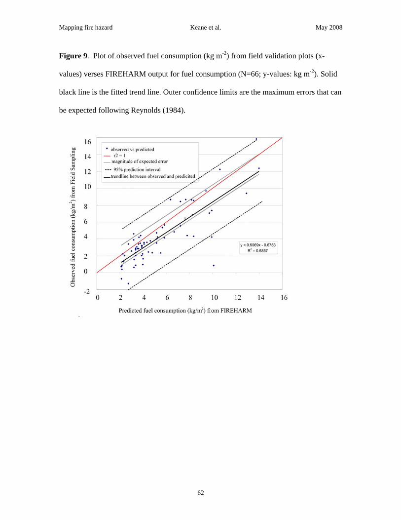
Mapping fire hazard Keane et al. May 2008
Figure 9. Plot of observed fuel consumption (kg m-2) from field validation plots (x-
values) verses FIREHARM output for fuel consumption (N=66; y-values: kg m-2). Solid
black line is the fitted trend line. Outer confidence limits are the maximum errors that can
be expected following Reynolds (1984).
62

Mapping fire hazard Keane et al. May 2008
Figure 10. Scatterplots of observed (plot data) with predicted (FIREHARM estimates)
for five fire hazard variables used for model validation along with quantile plots: a, b)
tree mortality, c,d) burn severity,e,f) scorch height, and g,h) flame lengths.
63