A meshless modeling of dynamic strain localization in quasi-brittle

materials using radial basis function networks

P. Le∗ N. Mai-Duy† T. Tran-Cong‡ and G. Baker§

October 22, 2008

Abstract

This paper describes an integrated radial basis function network (IRBFN) method for thenumerical modelling of the dynamics of strain localization due to strain softening in quasi-brittlematerials. The IRBFN method is a truly meshless method that is based on an unstructuredpoint collocation procedure. We introduce a new and effective regularization method to enhancethe performance of the IRBFN method and alleviate the numerical oscillations associated withweak discontinuity at the elastic wave front. The dynamic response of a one dimensional bar isinvestigated using both local and non-local continuum models. Numerical results, which comparefavourably with those obtained by the FEM and the analytical solutions for a local continuummodel, demonstrate the efficiency of the present IRBFN approach in capturing large strain gradientsencountered in the present problem. keyword Strain localization, IRBFN, wave propagation,softening materials, quasi-brittle materials.

1 Introduction

In many engineering structures subjected to extreme loading conditions, the initially smooth dis-tribution of strain may change into a highly localised one. Typically, extremely high strains mayoccur within a very narrow zone while the remaining part of the structure experiences unloading.Such strain localization usually can be caused by geometrical nonlinearities (e.g., necking of metallicbars) or by material instabilities (e.g., micro-cracking). Mathematically, the onset of strain local-ization, in the context of a rate-independent local continuum model, leads to loss of hyperbolicityof the governing partial differential equations, i.e. when the matrix of tangent modulus ceases tobe positive-definite. From a computational point of view, the loss of hyperbolicity causes numericaldifficulties since the mathematical model becomes ill-posed (localised zone of zero volume). To reg-ularize the ill-posed problems, a number of localization limiters have been developed to ensure thatlocalised zones have a finite volume and the problem becomes well-posed. Examples of localisationlimiters include non-local models, rate-dependent models, gradient-dependent models, visco-plasticmodels, damage-based models, cohesive crack models, smear crack models and Cosserat continuummodel.

For one dimensional problems (softening bars), some closed-form exact and approximate so-lutions have been developed by many authors, including, for example, [Bazant and Belytschko(1985); Sluys (1992); Xin and Chen (2000); Armero and Park (2003)] for the evolution of dynamicstrain localization via rate-independent local constitutive models. The above closed-form solutions

∗CESRC, University of Southern Queensland, Toowoomba, QLD 4350, Australia.†CESRC, University of Southern Queensland, Toowoomba, QLD 4350, Australia.‡CESRC, University of Southern Queensland, Toowoomba, QLD 4350, Australia.§DVC(S), University of Southern Queensland, Toowoomba, QLD 4350, Australia.

1

demonstrated that one of the following two cases is possible. First, if the behavior of the tensilebars is fully elastic, the displacement field is C0 continuous, the strain field is discontinuous andthe discontinuities propagate as incident as well as reflected waves. Second, if localization occurs,the mathematical model becomes ill-possed in the context of a rate-independent local continuummodel as stated above. Hence, numerical methods are not able to capture the solutions using rate-independent local constitutive models [Bazant and Belytschko (1985); Sluys (1992); Askes et al.(1998)]. Moreover, even if a localization limiter is applied, for an accurate description of the local-ized zone, a very fine computational mesh is needed, since the strain gradients are very high withinlocalized zones. Hence, robust numerical methods are required to analyze such strain localizationphenomena. In general, the position of the localization zone is unknown, therefore, an automaticmesh adaptive procedure is required to increase the efficiency of the numerical method. However,the polynomial approximations in FEM can poorly capture the non-smooth transition between theunloading region with almost constant strain and the localization zone with rapid strain increase[Patzak and Jirasek (2003)] and the FEM results are very sensitive to the computational grids. Theextended finite element method [Patzak and Jirasek (2003)], which incorporates special enrichmentfunctions into the shape functions, produces better results, however, the asymptotic solutions arerequired to be known in advance. Owing the non-local nature of approximations used [Atluri andZhu (1998); Li and Liu (2000); Batra and Zhang (2004); Atluri and Shen (2002); Han and Atluri(2003, 2004); Le et al. (2007); Wen and Hon (2007)], meshless methods possess some advantages inmodelling such strain localization problems and provide more continuous solutions than the piece-wise continuous ones obtained from FEM. Thus meshless methods offer effective solutions to themesh alignment sensitivity in strain localization modelings.

In this study, we report a new numerical method based on radial basis function networks, atruly meshless method, for the analysis of the dynamics of strain localization in 1D problems.The present indirect/integral radial basis function network (IRBFN) method is based on (i) theuniversal approximation property of RBF networks, (ii) exponential convergence characteristics ofthe chosen multiquadric (MQ) RBF, (iii) a simple point collocation method of discretisation ofthe governing equations, and (iv) an indirect/integral (IRBFN) rather than a direct/differential(DRBFN) approach [Kansa (1990)] for the approximation of functions and derivatives. For theDRBFN, Madych and Nelson (1990) showed that the convergence rate is a decreasing function ofderivative order. Since the introduction of the IRBFN approach by [Mai-Duy and Tran-Cong (2001,2005); Kansa et al. (2004); Ling and Trummer (2004); Mai-Duy, Mai-Cao and Tran-Cong (2007);Mai-Duy, Khennane and Tran-Cong (2007)], based on the theoretical result of Madych and Nelson[Madych and Nelson (1990)], concluded that the decreasing rate of convergence can be avoidedin the IRBFN approach. Furthermore, the integration constants arisen in the IRBFN approachare helpful in dealing with problems with multiple boundary conditions [Mai-Duy and Tran-Cong(2006)]. However, being a global and high order approximation method, RBF-based methods alsosuffer from the Gibbs phenomenon where numerical oscillations occur around a jump discontinuityor near a boundary [Jung (2007)], with consequential deterioration of convergence rate, accuracyand stability. In the case of approximation methods based on multiquadric radial basis function(MQ-RBF), several approaches have been developed to attenuate the Gibbs oscillations. For ex-ample, Jung (2007) proposed an adaptive piecewise linear basis functions in the vicinity of thediscontinuity; Driscoll and Heryudono (2007) suggested an adaptive residual subsampling methodsand Le et al [Le et al. (2007)] offered a new coordinate mapping (for boundary-layer problems). Inaddition, we introduce a new and effective regularization method based on the IRBFN to alleviatenumerical oscillations, which enhances the performance of the present method in dealing with weakdiscontinuities associated with the strain localization process. The paper is organized as follows.The physical problem and its mathematical model are defined in section 2. The numerical formula-tion for the mathematical model is presented in section 3 which is followed by numerical examplesin section 4. Section 5 concludes the paper.

2 Problem definition

Consider a solid bar of of length 2L, with a unit cross sectional area and mass ρ per unit length asshown in Figure 1. Let the bar be loaded by forcing both ends to move simultaneously outward,with a constant opposite velocity of magnitude c. The governing equations are described as follows.

2

Figure 1: A model of uniform bars.

The momentum equation is given by

ρ∂2u(x, t)

∂t2=

∂σ(x, t)

∂x, (1)

where x is the coordinate measured from the mid-point of the bar, −L ≤ x ≤ L; t is time 0 ≤ t ≤tmax; u(x, t) is the displacement in x the direction and σ(x, t) is the stress.

The material behaviour is described by a bilinear constitutive law as presented in Figure 2,which exhibits elastic behavior with Young’s modulus E up to strain εp at the peak stress fy

(strength), followed by strain-softening (line PF ), which has a negative slope Et up to εf , wherethe stress has a value of zero, finally, followed by a nearly horizontal tail of a very small positiveslope Ef .

Figure 2: A constitutive relation for quasi-brittle materials.

The constitutive relation is thus given by

△σ(x, t) = E△ε, (2)

in which ǫ = ǫ(x, t) = ∂u(x,t)∂x

is the strain and E is the slope of the stress-strain relation, definedby

E =

E, if ε ≤ εp,

Et, if εp ≤ ε ≤ εf ,

Ef , if ε ≥ εf .

(3)

The boundary conditions are

u(x = −L, t) = −ct; u(x = L, t) = ct, for t ≥ 0. (4)

The initial solutions are taken as follows

u(x, t = 0) = 0 and∂u(x, t = 0)

∂t= 0, for − L ≤ x ≤ L. (5)

3

Due to symmetry, the problem is equivalent to a bar fixed at x = 0. Thus the boundary conditionsfor a half model now become

u(x = −L, t) = −ct; u(x = 0, t) = 0, for t ≥ 0. (6)

The governing equations are non-dimensionalised using the following scheme: characteristiclength a; characteristic time T = a

ve, where ve =

√

E/ρ is the elastic wave speed; characteristicstress σc = E; velocities are normalised by ve, e.g. c/ve is the dimensionless loading velocity at theends of the bar. The dimensionless momentum equation is given by

∂2u(x, t)

∂t2=

(

ET 2

ρa2

)

∂σ(x, t)

∂x,

=

(

E

E

)

γ2 ∂ε(x, t)

∂x, (7)

where E is given in Equation 3, γ =√

ET 2

ρa2 = veTa

.

In the remaining of the paper, for brevity, in addition to (u, x, t, σ), c and L are now dimen-sionless quantities.

3 Numerical formulation

Consider an initial-boundary-value problem governed by the second order PDE

∂u

∂t= q1

∂2u

∂x2+ q2

∂u

∂x+ q3u + q4, (8)

where q1, q2, q3 and q4 are the coefficients, 0 ≤ t ≤ T and xmin ≤ x ≤ xmax, with the boundaryand initial conditions

u(t, x = xmin) = u1, (9)

∂u

∂x|(t,x=xmax) = u′

N , (10)

u(0, x) = g(x), (11)

in which u1 and u′N are given values, and g(x) is a known function.

3.1 Spatial discretisation

In the indirect RBF method (see [Mai-Duy and Tran-Cong (2001, 2005); Mai-Duy (2005); Mai-Duy and Tanner (2005)]), the formulation of the problem starts with the decomposition of thehighest order derivative under consideration into RBFs. The derivative expression obtained is thenintegrated to yield expressions for lower order derivatives and finally for the original function itself.The present work is concerned with the approximation of a function and its derivatives of order upto 2, the formulation can be thus described as follows [Mai-Cao and Tran-Cong (2005); Le et al.

4

(2007)]

d2u(x, t)

dx2=

m∑

i=1

wi(t)gi(x) =

m∑

i=1

wi(t)H[2]i (x), (12)

du(x, t)

dx=

∫ m∑

i=1

wi(t)gi(x)dx + c1(t)

=

m∑

i=1

wi(t)

∫

gi(x)dx + c1(t)

=

m∑

i=1

wi(t)H[1]i (x) + c1(t), (13)

u(x, t) =

m∑

i=1

wi(t)

∫

H[1]i (x)dx + c1(t)x + c2(t)

=

m∑

i=1

wi(t)H[0]i (x) + c1(t)x + c2(t), (14)

where m is the number of RBFs, {gi(x)}mi=1 is the set of RBFs, {wi(t)}

mi=1 is the set of corresponding

network weights to be found and {H[j]i (x)}m

i=1 (j = 0, 1) are new basis functions obtained fromintegrating the radial basis function gi(x) once or more times. The multiquadrics function ischosen in the present study

gi(x) =√

(x − ci)2 + a2i , (15)

where ci is the RBF centre and ai is the RBF width. The width of the ith RBF can be determinedaccording to the following simple relation

ai = βdi, (16)

where β is a factor, β > 0, and di is the distance from the ith centre to its nearest centre. Tohave the same coefficient vector as Equation 14, Equation 12 and Equation 13 can be rewritten asfollows

d2u(x, t)

dx2=

m∑

i=1

wi(t)H[2]i (x) + c1(t).0 + c2(t).0, (17)

du(x, t)

dx=

m∑

i=1

wi(t)H[1]i (x) + c1(t).1 + c2(t).0. (18)

Here we choose the RBF centres ci to be identical to the collocation points xi, i.e. {ci}mi=1 = {xi}

Ni=1.

The evaluation of Equation 17, Equation 18 and Equation 14 at a set of N collocation points leadsto

u′′(t) = H[2]w(t), (19)

u′(t) = H[1]w(t), (20)

u(t) = H[0]w(t), (21)

where

u′′(t) =

[

∂2u1(t)

∂x2,∂2u2(t)

∂x2, . . . ,

∂2uN(t)

∂x2

]T

, (22)

u′(t) =

[

∂u1(t)

∂x,∂u2(t)

∂x, . . . ,

∂uN(t)

∂x

]T

, (23)

u(t) = [u1(t), u2(t), . . . , uN (t)]T , (24)

H[2] =

H[2]1 (x1) H

[2]2 (x1) · · · H

[2]N (x1) 0 0

H[2]1 (x2) H

[2]2 (x2) · · · H

[2]N (x2) 0 0

......

. . ....

......

H[2]1 (xN ) H

[2]2 (xN ) · · · H

[2]N (xN ) 0 0

, (25)

5

H[1] =

H[1]1 (x1) H

[1]2 (x1) · · · H

[1]N (x1) 1 0

H[1]1 (x2) H

[1]2 (x2) · · · H

[1]N (x2) 1 0

......

. . ....

......

H[1]1 (xN ) H

[1]2 (xN ) · · · H

[1]N (xN ) 1 0

, (26)

H[0] =

H[0]1 (x1) H

[0]2 (x1) · · · H

[0]N (x1) x1 1

H[0]1 (x2) H

[0]2 (x2) · · · H

[0]N (x2) x2 1

......

. . ....

......

H[0]1 (xN ) H

[0]2 (xN ) · · · H

[0]N (xN ) xN 1

, (27)

andw(t) = [w1(t), ..., wN (t), c1(t), c2(t)]

T . (28)

From an engineering point of view, it would be more convenient to work in the physical space.Owing to the presence of integration constants, the process of converting the networks-weightspace into the physical space can also be used to implement Neumann boundary conditions. Withthe boundary conditions Equation 9 and Equation 10, the conversion system can be written as

(

u(t)u′

N (t)

)

= Cw(t), (29)

where C is the conversion matrix of dimension (N + 1) × (N + 2) that comprises the matrix H[0]

and the last row of H[1]. Solving Equation 29 yields

w(t) = C−1

(

u(t)u′

N (t)

)

. (30)

By substituting Equation 30 into Equation 19 and Equation 20, the values of the second and firstderivatives of u with respect to x are thus expressed in terms of nodal variable values and Neumannboundary values

u′′(t) = H[2]C−1

(

u(t)u′

N(t)

)

= D[2]

(

u(t)u′

N (t)

)

, (31)

u′(t) = H[1]C−1

(

u(t)u′

N (t)

)

= D[1]

(

u(t)u′

N(t)

)

. (32)

Making use of Equation 31 and Equation 32, Equation 8 can be transformed into the followingdiscrete form

du(t)

dt= q1u

′′(t) + q2u′(t) + q3u(t) + q4, (33)

ordu

dt= q1D

[2]

(

u(t)u′

N (t)

)

+ q2D[1]

(

u(t)u′

N(t)

)

+ q3u(t) + q4, (34)

where q4 = [q4, q4, . . . q4]T

is an N × 1 vector, and

du

dt=

[

du1(t)

dt,du2(t)

dt, . . . ,

duN (t)

dt

]T

. (35)

Since the values of u1 and u′N are given, the unknown vector becomes

[u2(t), u3(t), . . . , uN(t)]T , (36)

and hence, the first row in Equation 34 will be removed from the solution procedure. The remainderof Equation 34 can be integrated in time by using standard solvers such as the Runge-Kuttatechnique.

6

3.2 Regularization of IRBFNs and capturing of discontinuous strains

When the displacement field is C0 continuous (e.g., across a bi-material interface or strain local-ization); it was found to be difficult to capture accurately the resultant discontinuous strains withconventional FEM. The latter can be improved with the introduction of enriched FEM [Patzak andJirasek (2003)], however, mesh alignment sensitivity remains a drawback at least for quadrilateralsand embedded discontinuity methods [Li and Liu (2000)]. On the other hand, several meshfreemethods used special shape functions to account for the jump across a discontinuity [Krongauz andBelytschko (1998); Kim et al. (2007)], which seem to work well if the location of discontinuities areknown. It will be seen that the present IRBFN method can capture strain discontinuities withoutsuffering any mesh-alignment sensitivities (IRBFN is a truly meshless method) and without havingto know the location of discontinuities in advance. However, being a global and high order ap-proximation, the RBFN still produce some oscillations around the discontinuity (Figure 3). In thisstudy we introduce a new approach where RBFNs can be further regularised to alleviate oscillatorybehaviours near such discontinuities.

−50 −40 −30 −20 −10 0 10 20 30 40 50−0.2

0

0.2

0.4

0.6

0.8

1

1.2

x

exact solutionIRBFN approximationIRBFN regularization

Figure 3: Regularization of IRBFNs.

With noisy data, the generalization performance of RBFNs can be improved using regularizationtechniques presented in [Orr (1995b)], which are adapted here for IRBFNs. Let

{

(x = {xi}Ni=1, y = {yi}

Ni=1)

}

denote the set of input and f(x) the output in the present IRBFN method, the sum-squared-erroris

S =

N∑

i=1

(yi − f(xi))2, (37)

where N is the number of input data points, f(xi) is the approximate solution given by Equation 14(or Equation 21 in matrix form). The output sensitivity to noisy inputs is minimised by augmentingthe sum-squared-error with a smoothing term [Orr (1995b)] as follows.

C =N

∑

i=1

(yi − f(xi))2 + λ

m∑

j=1

w2j , (38)

where C is a cost function, m is the number of RBF centres, wj are the network weights, λ is anon-negative regularization parameter. An optimal weight vector w can be found by minimizingC in Equation 38 with respect to network weights {wj}

N

j=1 as follows. Differentiating the cost

function C with respect to the network weights {wj}N

j=1 yields

∂C

∂wj

= −2

N∑

i=1

(yi − f(xi))∂f(xi)

∂wj

+ 2λ

m∑

j=1

wj . (39)

7

From Equation 14 or Equation 21, ∂f(xi)∂wj

in Equation 39 can be found simply as

∂f(xi)

∂wj

= H[0]j (xi), (40)

or in compact form∂f

∂wj

= h[0]j , (41)

wheref = [f(x1), f(x2), ..., f(xN )]

T, (42)

and

h[0]j =

[

H[0]j (x1), H

[0]j (x2), ..., H

[0]j (xN )

]T

. (43)

Note that vector h[0]j is the j-th column of the matrix H[0] in Equation 27. Substituting Equation

41 into Equation 39 and equating the results to zero lead to

N∑

i=1

f(xi)H[0]j (xi) + λwj =

N∑

i=1

yiH[0]j (xi). (44)

There are m such equations corresponding to m radial basis functions, 1 ≤ j ≤ m, each representsone constraint on the solution. The resultant system of linear equations like Equation 44 can berewritten in matrix form,

(

H[0])T

f + λIm+2w =(

H[0])T

y, (45)

in which Im+2 is an identity matrix of size (m + 2) × (m + 2). Solving Equation 45 leads to thevector of optimal weights

w = A−1

(

H[0])T

y, (46)

where

A =(

H[0])T

H[0] + λIm+2. (47)

Since the performance of the IRBFN regularization completely depends on the regularization pa-rameter λ, an optimal λ must be identified to minimise the error. A number of methods predictingan optimal value of λ automatically have been developed [Orr (1995a,b, 1996)] including the re-estimation method using different error prediction criteria, (e.g. cross-validation, generalized cross-validation, Bayesian information criterion, final prediction error, unbiased estimate of variance). Inthe present work, the generalized cross-validation (GCV) error prediction criterion is employed asfollows.

σ2 =N yT P2y

[trace(P)]2, (48)

where σ2 is the variance estimate, N is the number of input data points, P is the projectionmatrix, which is defined by

y − f = y − H[0]A−1

(

H[0])T

y = Py, (49)

in which P = IN −H[0]A−1(

H[0])T

, IN is an identity matrix of size N ×N . Thus P relates to thesum-square-error S by

S = yT P2y, (50)

and the cost function C byC = yT Py. (51)

Since all the above error prediction criteria relate nonlinearly to λ, a method of nonlinearoptimization is required for the estimation of λ. Any standard technique of nonlinear optimizationsuch as the Newton method can be used in this circumstance. Alternately, the optimal value of λcan automatically be determined by a simple iterative procedure [Orr (1996)] as follows.

8

By differentiating the GCV error prediction and setting the results to zero, a nonlinear equation ofλ can be obtained. After some mathematical manipulations, λ can be found iteratively as

λ =yT P2y trace

(

A−1 − λA−2)

wT A−1w trace(P), (52)

where the right hand side contains λ (explicitly as well as implicitly through A−1 and P). Theiterative procedure is started with an initial value of λ for the computation of the right hand side,which is a new estimate of λ, and the process is repeated until convergence.

0 0.1 0.2 0.3 0.4 0.5 0.6 0.7 0.8 0.9 1−1.5

−1

−0.5

0

0.5

1

1.5

x

y

RBFN regularization

input noisesexact solutionDRBFNIRBFN

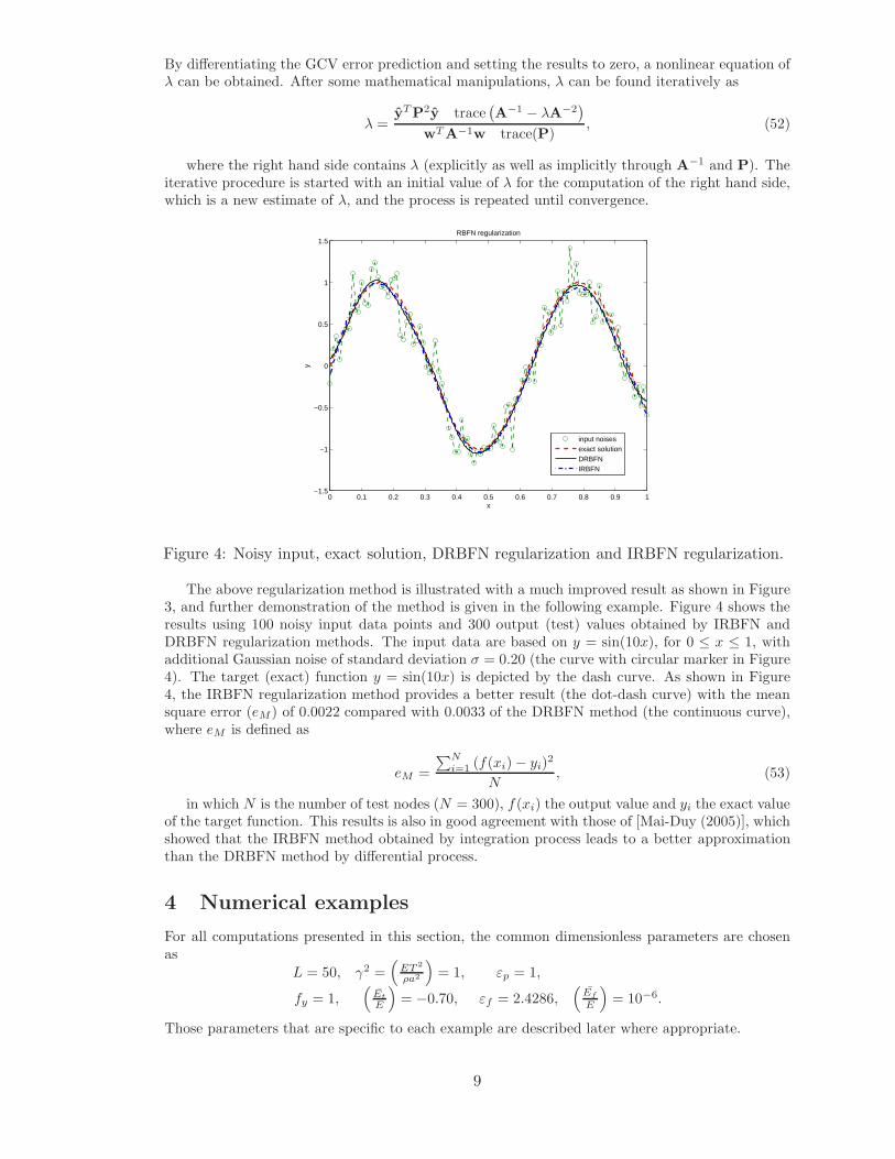
Figure 4: Noisy input, exact solution, DRBFN regularization and IRBFN regularization.

The above regularization method is illustrated with a much improved result as shown in Figure3, and further demonstration of the method is given in the following example. Figure 4 shows theresults using 100 noisy input data points and 300 output (test) values obtained by IRBFN andDRBFN regularization methods. The input data are based on y = sin(10x), for 0 ≤ x ≤ 1, withadditional Gaussian noise of standard deviation σ = 0.20 (the curve with circular marker in Figure4). The target (exact) function y = sin(10x) is depicted by the dash curve. As shown in Figure4, the IRBFN regularization method provides a better result (the dot-dash curve) with the meansquare error (eM ) of 0.0022 compared with 0.0033 of the DRBFN method (the continuous curve),where eM is defined as

eM =

∑Ni=1 (f(xi) − yi)

2

N, (53)

in which N is the number of test nodes (N = 300), f(xi) the output value and yi the exact valueof the target function. This results is also in good agreement with those of [Mai-Duy (2005)], whichshowed that the IRBFN method obtained by integration process leads to a better approximationthan the DRBFN method by differential process.

4 Numerical examples

For all computations presented in this section, the common dimensionless parameters are chosenas

L = 50, γ2 =(

ET 2

ρa2

)

= 1, εp = 1,

fy = 1,(

Et

E

)

= −0.70, εf = 2.4286,(

Ef

E

)

= 10−6.

Those parameters that are specific to each example are described later where appropriate.

9

4.1 Wave propagation in fully elastic bars

A uniform bar is loaded by an extensional velocity c of the two ends as shown in Figure 1. Lon-gitudinal elastic wave propagation precedes strain localisation and is considered in this example.Moreover, if c satisfies the condition c ≤ εp/2, the behaviour of the bar is purely elastic over thewhole computational domain [Bazant and Belytschko (1985)]. The differential equation of motionEquation 7 reduces to (in dimensionless form)

∂2u(x, t)

∂t2= γ2 ∂2u(x, t)

∂x2, (54)

which is hyperbolic. The exact solution of Equation 54 for the given boundary conditions Equation4 and the initial solutions Equation 5 can be found in [Bazant and Belytschko (1985)] and presentedfor the displacement u and strain ε as follows.

u = −c 〈γt − (x + L)〉 + c 〈γt + (x − L)〉 , 0 ≤ t ≤

(

1

γ

)

2L, (55)

where the symbol 〈〉 is defined by

〈A〉 =

{

A, if A ≥ 0,

0, if A < 0,(56)

and

ε =∂u

∂x= c [H (γt − (x + L))] + c [H (γt + (x − L))] , (57)

in which H denotes the Heaviside step function, defined by

H(x) =

{

1, if x ≥ 0,

0, if x < 0.(58)

The governing equation Equation 54 involves second-order derivatives of both space and time, andit is convenient to decouple it into a system of first-order equations in both space and time byintroducing new variables r and s as follows. Let

r = γ∂u

∂x, s =

∂u

∂t, (59)

and Equation 54 is thus equivalent to the system of equations

∂r

∂t= γ

∂s

∂x, (60)

∂s

∂t= γ

∂r

∂x, (61)

subject to the corresponding boundary conditions

s(−L, t) = −c, s(L, t) = c, ∀t ∈

[

0,

(

1

γ

)

2L

]

, (62)

and the initial solutionsr(x, 0) = 0, s(x, 0) = 0, ∀x ∈ [−L, L]. (63)

To reduce the computational cost, a half model is analyzed in this section. The equivalent boundaryconditions of the half model are

s(−L, t) = −c, s(0, t) = 0, ∀t ∈

[

0,

(

1

γ

)

2L

]

, (64)

The numerical formulation presented in section 3 is used for solving the system of equations Equa-tion 60 and Equation 61 with the boundary conditions Equation 64 and the initial solutions Equa-tion 63, with c = 0.45εp. The forward Euler formula is used to perform time integration. To satisfythe CFL condition (△t ≤ 1

γ△x), the time step is chosen as △t = 10−2 1

γ△x in this example. The

10

results presented in this example are achieved with 80 uniform collocation points and β = 1 inEquation 16. Computations are also carried out with 20, 40, 60 and 100 uniformly distributedcollocation points. The obtained solution essentially converges when 40 or more collocation pointsare used. Figures 5, 6 and 7 show the evolution of the displacement and strain, the numericalresults and the exact solutions are plotted on the same graphs. First, the displacement and strainwaves propagate from the ends to the center of the bar until these incident waves meet each other

at the center at time t =(

1γ

)

L. The zero-th order continuous displacement leads to the strain

discontinuity whose position evolves with time as shown in the above figures. As a result of thecollision of the two incident waves (at x = 0), an abrupt jump of value of strain appears at x = 0(Figure 8), the strain magnitude is doubled, and the reflection waves propagate outwards to theends as displayed in Figures 5(e)-(f)-(g)-(h), 7 and 8. The obtained results by the present IRBFNmethod are in good agreement with the analytical solutions as shown in Figures 5-8.

It is shown that the IRBFN can capture the discontinuous strain in this example, however,there are some oscillations due to the violation of the smoothness assumption inherent in theRBFN approximation. This situation can be improved with regularisation as discussed in section3.2. When the regularisation parameter λ is set to be equal to 0.07135, it can be seen that theobtained strains shown on the right columns in Figures 6 and 7 are much smoother and closer tothe exact solutions than those by the standard IRBFN method shown on the left columns of thesame figures. Thus, good results are achieved with a general global regularisation of the IRBFNsin contrast with other numerical approaches (discussed in section 3.2) where special treatmentsmust be applied at the elemental level (extended FEM) or special shape functions must be used.Moreover, these special treatments require a priori knowledge of the location of discontinuities whilethe present IRBFN method does not.

4.2 Wave propagation and strain localization in strain-softening bars:

local continuum model

In this example, the problem defined in section 2 is considered with the prescribed velocities at theends have c = 0.85εp, which is above the critical value of 0.5εp. The behaviour of the bar is elasticuntil the incident waves meet at the center of the bar (i.e. for 0 ≤ t ≤ L) as discussed in section 4.1.Right after the collision of the incident waves, the strain is doubled to 2c = 1.7εp, causing strainsoftening and strain localization. From the onset of localization, the computational domain can bedivided into two regions with different behaviors: the strain softening and localization zone and theelastic zone. For the elastic domain, the momentum equation Equation 7 takes the hyperbolic formof Equation 54 which is solved in the same manner as presented in section 4.1. For the localizedzone, the momentum equation becomes elliptic and is solved by a scheme described as follows.

The elliptic momentum equation of the localized zone is

∂2u(x, t)

∂t2= −µ2 ∂2u(x, t)

∂x2, (65)

in which µ2 = |Et|E

ET 2

ρa2 , and |Et| is the absolute value of Et. Equation 65 can be decoupled into asystem of first-order equations in both time and space by letting

r = −µ∂u

∂x, s =

∂u

∂t, (66)

resulting in a system of equations in r and s for the strain-softening zone given by

∂r

∂t= −µ

∂s

∂x, (67)

∂s

∂t= µ

∂r

∂x. (68)

At the end of the softening process, fracture and rupture will probably occur, however, a fracturecriterion is not included in present study, so the material is assumed to be elastic again with a verysmall elastic modulus Ef/E = 10−6. The governing equations in this stage are the same as thosein section 4.1, except that the modulus E is replaced by Ef . As before, only a half model needs bediscretised (in this case with 80 uniformly distributed nodes). The resultant system of equations

11

is integrated in time by using the forward Euler formula as in section 4.1, where the time stepis taken as △t = 0.25 × 10−4 △x

γin this example. The solution of Equation 67 and Equation

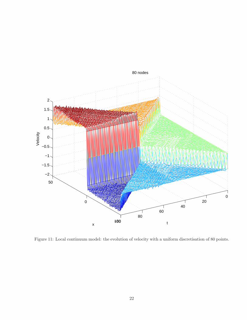
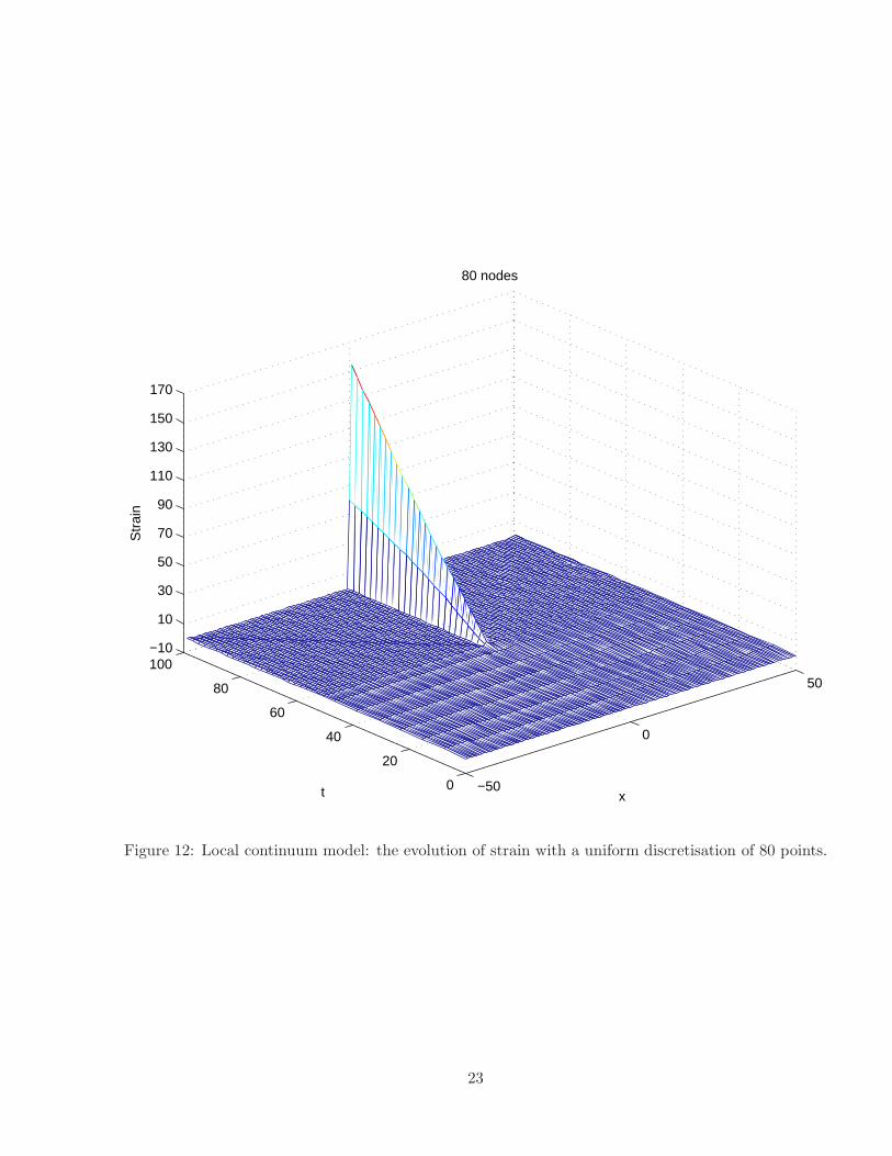
68 clearly shows the onset of strain localization, characterized by the sudden jump in velocity,displacement, strain and the rapid descent of stress in the localized zone as exhibited in Figure9 which depicts the evolution of velocity, displacement, strain and stress at the collocation pointx = −0.6329, which is the nearest point to the x = 0 node. In Figure 9(d), the stress profile isslightly oscillatory until the loading waves are about to meet. Upon the collision of the incidentwaves, the stress increases rapidly to the elastic limit fy then decreases as rapidly down to zeroagain due to strain-softening. The speedy drop of the stress level is accompanied by the abruptjump in velocity and rapid increase in displacement and strain as exhibited in Figure 9(c)-(a)-(b),respectively. Unstable development follows as the localized zone is unable to carry load while thevelocity is increasing, the displacement and strain are growing rapidly, two halves of the bar aremoving increasingly in two opposite directions like in mode I crack as shown in Figure 10. In thenext stage of evolution, the velocity and stress increase very slightly while the displacement andstrain are growing continuously and quickly because of elastic loading as can be seen in Figure 9.The steep profiles of stress, velocity and strain are well captured by the present explicit method,although with smaller time steps in comparison with other implicit methods. Figures 10-Fig.12depict the spatio-temporal evolution of the displacement, velocity and strain, respectively, whileFigures 13-15 show the spatial distribution of velocity, stress, displacement and strain, respectively,at several time instants. The solutions of the elliptic equations yield a standing wave, which is notable to extend outside the localised zone, as illustrated by the strain wave displayed in Figures 12and 15, and the displacement wave in Figures 10 and 14 as well. When softening occurs, which isthe case here, the localised strain softening zone causes reflection waves travelling backwards fromthe localised front (x = 0), due to sudden unloading.

Figures 10 and 14 expose the development of displacement which grows rapidly as a standingwave confined in a very narrow zone. Correspondingly, the increasingly intensive strain within thelocalized zone is depicted in Figures 12 and 15. The velocity is doubled at the onset of localisationand reflected back from the localised zone as shown in Figures 11 and 13(a). Similarly, displacement,strain and stress waves also reflected from the localised zone. However, unlike the response inpurely elastic bars, the reflected strain wave is out of phase with, and therefore cancelling out theincident strain wave of the same magnitude. Due to the nature of the displacement waves thedisplacement field in the elastic region is C0 continuous (Figures 10 and 14). The point of C0

continuous displacement propagates along the elastic region in both directions depending on thestage of loading. Consequently, a discontinuity occurs in the profile of stress, velocity (Figure 13),and strain (Figure 15). The oscillatory behaviour of the stress is observed in Figure 13(b) whichwas also found in [Sluys (1992); Bazant et al. (1984)].

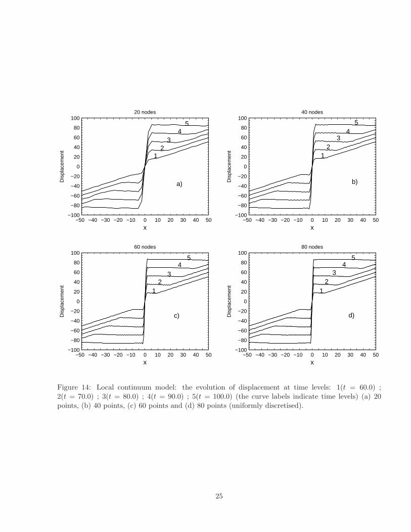
Although the results presented above correspond to an 80 point discretisation, computationis also carried out for 20, 40, 60, 100, 120 point discretisations. As the number of collocationpoints increases, the bandwidth of the localised zone decreases and the maximum strain increasesas shown in Figures 14 and 15, which is a trend predicted by the exact solution [Bazant andBelytschko (1985)]. However, the zero bandwidth and singular strain associated with the exactmodel solution cannot be expected to be captured by a numerical method. The obtained results inthis section compare favourably with those of the FEM [Sluys (1992); Bazant et al. (1984)]. It isworth noting that, unlike the FEM, the present method does not require a priori knowledge of thelocation of discontinuities which are well captured by a uniform discretisation.

4.3 Wave propagation and strain localization in strain-softening bars:

non-local continuum model

In this example, the material is described by a non-local continuum model based on strain aver-aging or non-local strain. In this model, the local equivalent strain ε is replaced by its non-localcounterpart obtained by a weighted average process over a spatial neighbourhood of each point ofinterest. The non-local strain ε is defined by

ε(x, t) =

∫

V

α(x, ξ)ε(ξ, t)dξ, (69)

where α(x, ξ) is a given non-local function. In an infinite body, the weight function is assumed todepend only on the distance r =‖ x−ξ ‖ between the “source” point ξ and the “receive” point x. In

12

the vicinity of a boundary, the weight function is usually rescaled such that the non-local operatordoes not change the uniform field, this means that the weight function satisfies the normalizingcondition

∫

V

α(x, ξ)dξ = 1, ∀x ∈ V. (70)

This can be achieved by setting

α(x, ξ) =α0(‖ x − ξ ‖)

∫

Vα0(‖ x − ζ ‖)dζ

, (71)

where α0(r) is an even and non-negative function of the distance r =‖ x − ξ ‖, monotonicallydecreasing for r ≥ 0. It is often taken as the piecewise polynomial bell-shaped function

α0(r) =

[

1 − r2

R2

]2

, if 0 ≤ r ≤ R,

0, if r > R,(72)

where R is a parameter related to the internal length of the material. Since R corresponds to themaximum distance of point ξ that affects the non-local average at point x, it is called the interactionradius [Patzak and Jirasek (2003)].

The stress-strain relation in Equation 2 becomes (in dimensionless form)

σ(x, t) =E

Eε(x, t), (73)

where ε is the non-local strain. Thus the stress in Equation 73 is also non-local. In order to evaluateε, it is necessary to compute ε(ξ, t) in Equation 69, which is accomplished as follows. After anIRBFN discretisation, the vectors of unknown nodal displacements and their corresponding firstand second derivatives with respect to x are given by Equation 21, Equation 32 and Equation 31,respectively. Thus, the first order derivative of the displacement with respect to x at an arbitrarypoint ξ can be written as follows.

∂u(ξ, t)

∂x= ε(ξ, t) = H [1](ξ)C−1u(t) = D[1](ξ)u(t), (74)

where C−1 and u(t) are given by Equation 30 and Equation 21, respectively. H [1](ξ) and D[1](ξ)are obtained in the same manner that leads to H[1] and D[1]in Equation 32, but with x = ξ.Substitution of Equation 74 into Equation 69 leads to

ε(x, t) =

∫ R

−R

α(x, ξ)D[1](ξ)u(t)dξ. (75)

Since the nodal variable vector u(t) is independent of the spatial variable, Equation 75 can berewritten as

ε(x, t) =

∫ R

−R

α(x, ξ)D[1](ξ)dξu(t) = B(x)u(t), (76)

where

B(x) =

∫ R

−R

α(x, ξ)D[1](ξ)dξ. (77)

The momentum equation Equation 7 becomes

∂2u(x, t)

∂t2=

(

E

E

) (

ET 2

ρa2

)

∂σ(x, t)

∂x, (78)

which, in the elastic case, reduces to

∂2u(x, t)

∂t2= γ2 ∂ε(x, t)

∂x. (79)

Since the stress and strain are non-local, a new system of governing equations is derived by decou-pling the momentum equation Equation 79 as follows. Let

r = γε(x) = γB(x)u(t), s =∂u

∂t. (80)

13

After discretisation, the unknown nodal vectors for r and s are, respectively,

r(t) = [r1(t), r2(t), . . . , rN (t)]T

, (81)

ands(t) = [s1(t), s2(t), . . . , sN(t)]T , (82)

where N is the number of collocation points.From Equation 80 and Equation 82, we have

∂u(t)

∂t= s(t). (83)

From Equation 79, Equation 80 and Equation 83, the following system of governing equations,which is equivalent to Equation 79 (i.e. the elastic case), is obtained

∂r(t)

∂t= γBs(t), (84)

∂s(t)

∂t= γ

∂r

∂x, (85)

whereB = [B(x1), B(x2), . . . , B(xN )]

T, (86)

with B(xi) =∫ R

−Rα(xi, ξ)D

[1](ξ)dξ, for i = ¯1, N

and ∂r

∂xis obtained by an IRBFN approximation as

∂r(t)

∂x= D[1]r(t). (87)

For the softening response, the corresponding system of governing equations is

∂r(t)

∂t= −µBs(t), (88)

∂s(t)

∂t= µ

∂r

∂x. (89)

The boundary and initial conditions for r and s are the same as those given in section 4.2. Ascan be seen in the previous two examples, the ramp-like spatial displacement profile results in adiscontinuous strain field which can be well captured by the present IRBFN method. However,when a non-local continuum model is used here, the smoothness of the equivalent non-local strainis adversely affected by noises that might exist in the neighbouring strain field. Thus it is found tobe advantageous to incorporate IRBFN regularisation into the general IRBFN formulation. Theeffect of such regularisation is illustrated by considering a ramp function given by

u(x) = xH(x), for − 50 ≤ x ≤ 50, (90)

where H is the Heaviside function defined in Equation 58. The exact solution of the first orderderivative of u(x) with respect to x is

ε(x) =∂u(x)

∂x= H(x). (91)

Let ε(x) denote the IRBFN approximation of ∂u(x)∂x

, which is determined by

ε(x) ≈∂u(x)

∂x= D[1](x)u(x), (92)

The weighted average of ε(x), denoted by ¯ε(x), is achieved by replacing ε(ξ, t) in Equation 69 byε(x)

¯ε(x) =

∫

V

α(x, ξ)ε(x)dξ, (93)

14

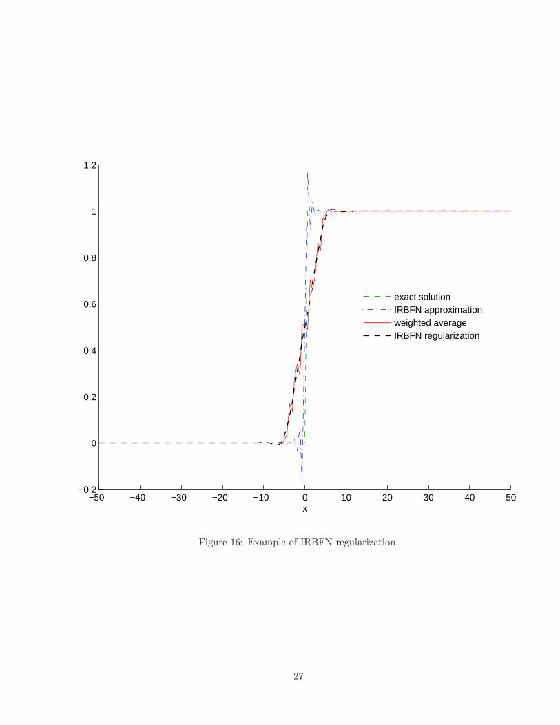
The domain is discretised with a uniform distribution of 161 collocation points. The IRBFNparameter β = 1 in Equation 16, the interaction radius R = 5 in Equation 93 which is integratedwith 11-point Gaussian quadrature, and the IRBFN regularisation parameter is λ = 3.391895. Theresults shown in Figure 16 demonstrate the effectiveness of the present method. In this figure,the exact solution ε(x) is represented by the Heaviside curve; the dot-dashed curve indicates theIRBFN solution ε(x); the solid curve represents the weighted average of the IRBFN approximation¯ε(x); the heavy dashed curve represents the regularised weighted average ¯ε(x). The above specificparameters, except λ which is dependent on the number of collocation points, are also used inobtaining the results described below.

Returning to the bar problem, the prescribed end velocities are the same as those given insection 4.2, i.e. c = 0.85εp. The time step is 10−3 △x

γ. Due to the presence of the non-local

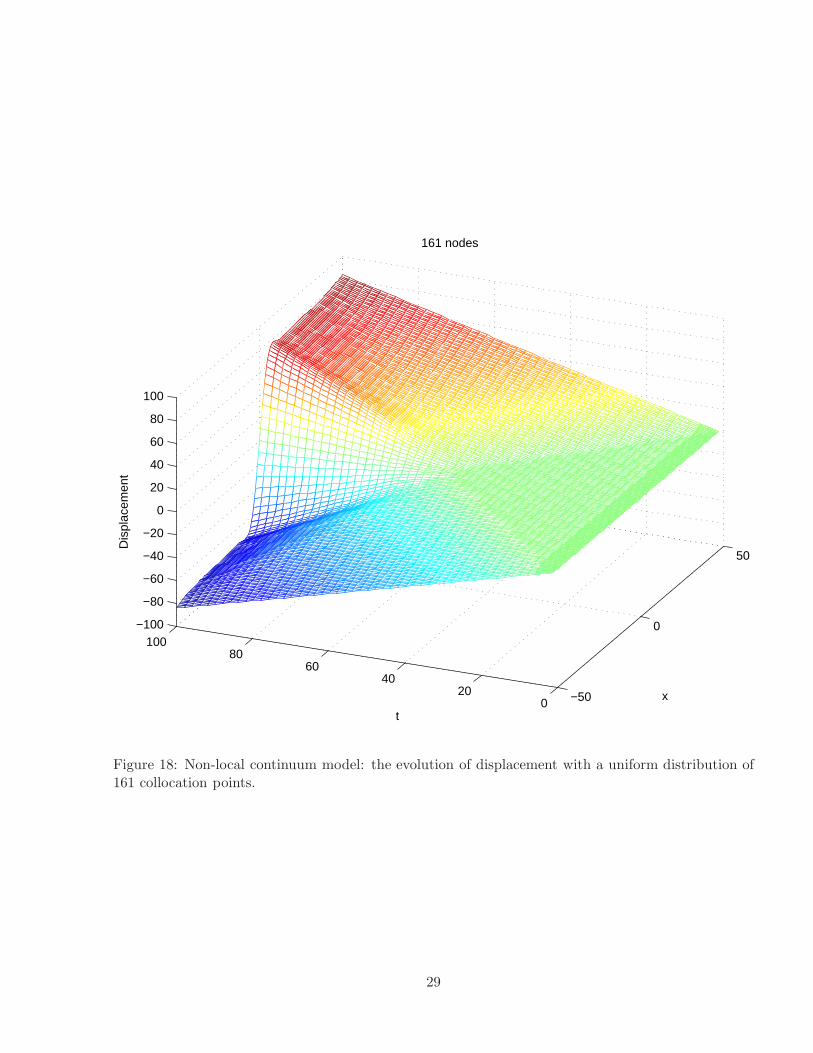
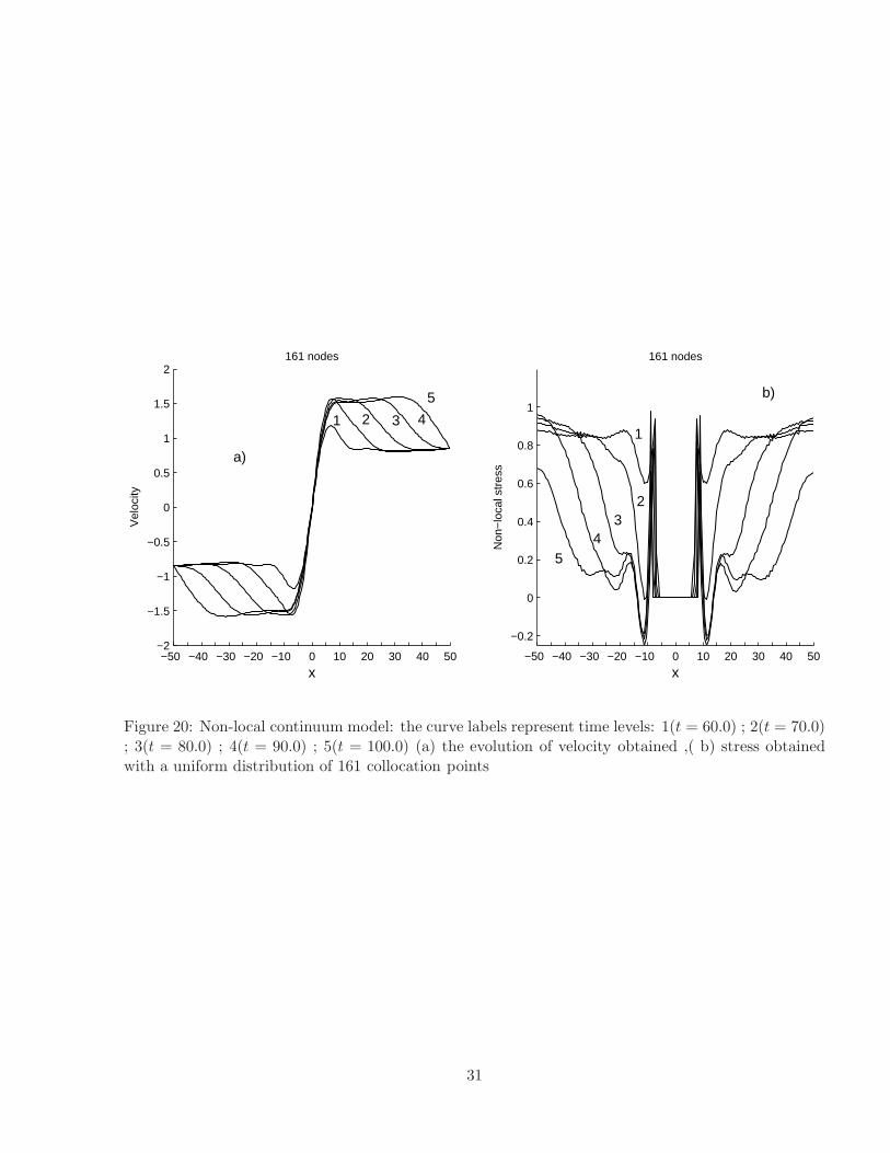
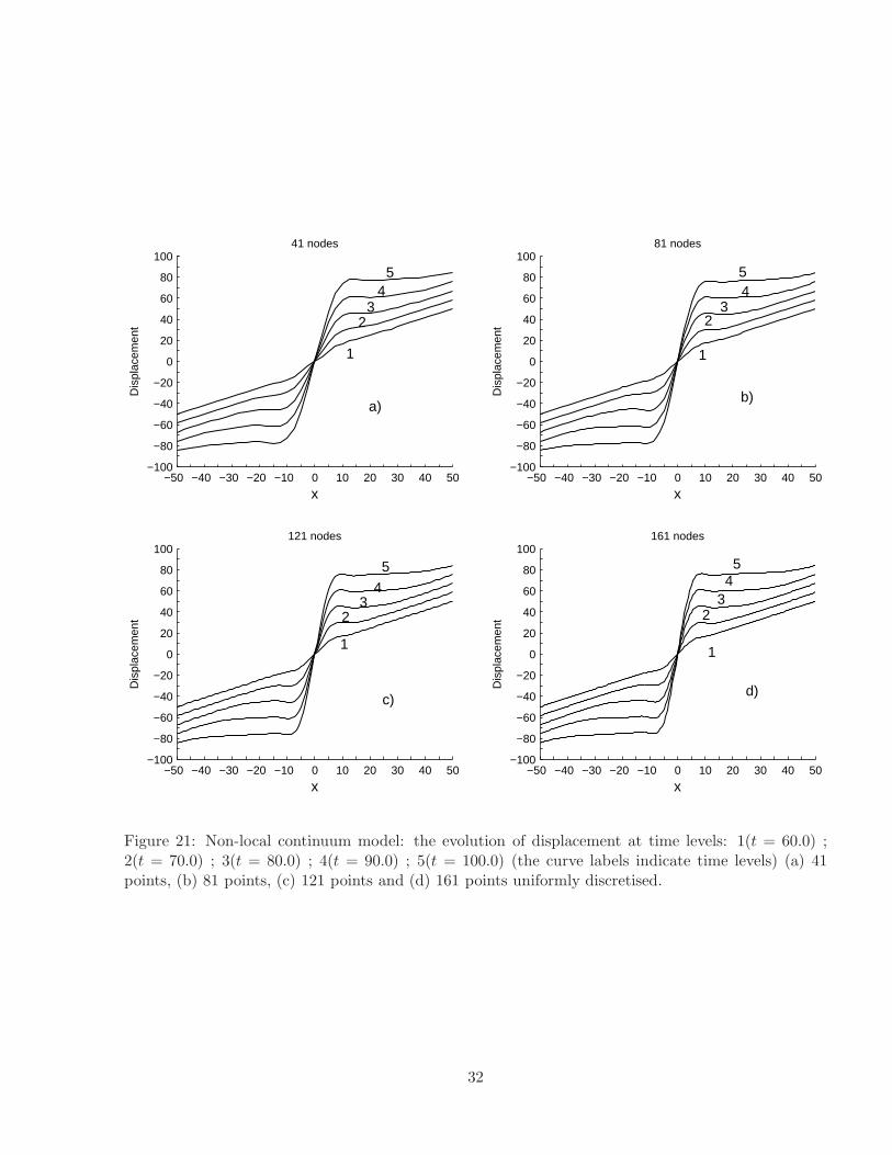
operator, the full model is analyzed. In fact, in the present computation s is regularised, insteadof ε, with similar end results. Figures 17-19 exhibit the evolution of velocity, displacement andnon-local strain, respectively. Owing to the properties of non-local weighted average operator, thenon-local continuum model yields much smoother response than the corresponding results obtainedwith a local continuum model, although the evolutionary profiles are similar as expected. The effectof standing wave can be seen in Figures 18-19 (continuous spatio-temporal representation), Figures21 and 22 (at selected times), which show that the growing displacement and strain are confined tothe localised zone. The bandwidth of the localized zone and the magnitude of the localized strainare finite, which is in contrast with the the results obtained with a local continuum model, wherethe exact solution is singular (zero bandwidth localised zone and hence infinite strain). After theonset of strain localization, the velocity, displacement, strain and stress waves reflected from thelocalised zone as shown in Figures 20-22. However, unlike the case of local continuum model, thewave profiles are smooth. In Figure 20(b), the profiles of stress indicate a complicated loading andunloading process after the initiation of strain localization. There are two narrow zones of highstress at the interfaces between the localized zone and the elastic regions. The standing wave causesthe stress to rise in the narrow zones until the elastic limit is reached when sudden unloading occursdue to strain softening effect.

Finally, convergence of the present numerical procedure is demonstrated in Figure 23 where thenon-local strain profiles (at t = 70.0) are displayed for a series of collocation points. As discretisationis refined, it can be seen that the bandwidth converges when the number of collocation points isabout 160 while the peak non-local strain varies by only 2.3% when the number of collocationpoints increases from 161 to 241. The slight variation of the peak non-local strain can be expectedsince the local strain at the centre of the band is singular.

5 Conclusion

An IRBFN meshless method is developed and used to simulate the dynamic strain localization ofa bar of quasi-brittle material under dynamic tensile loading. Both local and non-local continuummodels are used to describe the material behaviour. The method incorporates a new general andeffective regularization method. The enhanced IRBFN approach is able to alleviate the effectof noisy data and capture very well weak discontinuities typical of wave propagation and strainlocalisation. The present method is able to achieve these results using only uniformly distributedcollocation points and requiring no prior knowledge of the location of discontinuities.

acknowledgement This work is supported by the Australian Research Council. We would liketo thank the referees for their helpful comments.

15

−50 0 50

−5

0

5

x

u

t = 17.2685

−50 0 50−10

0

10

x

u

t = 26.1350

−50 0 50

−10

0

10

x

u

t = 35.0015

−50 0 50

−100

10

x

u

t = 43.8680

−50 0 50

−20

0

20

x

u

t = 61.6011

−50 0 50

−20

0

20

x

u

t = 70.4676

−50 0 50

−20

0

20

x

u

t = 79.3341

−50 0 50−40−20

02040

x

u

t = 92.6339

a) b)

c) d)

e) f)

g)h)

Figure 5: Fully elastic bars: the evolution of displacement, the continuous curves denote the IRBFNsolutions and the dash ones the exact solution.

16

−50 0 500

0.2

0.4

x

ε

t = 17.2685

−50 0 500

0.2

0.4

x

ε

t = 17.2685

−50 0 500

0.2

0.4

x

ε

t = 26.1350

−50 0 500

0.2

0.4

xε

t = 26.1350

−50 0 500

0.2

0.4

x

ε

t = 35.0015

−50 0 500

0.2

0.4

x

εt = 35.0015

−50 0 500

0.2

0.4

x

ε

t = 43.8680

−50 0 500

0.2

0.4

x

ε

t = 43.8680

a1) a2)

b1) b2)

d1)

c2)c1)

d2)

Figure 6: Fully elastic bars: the propagation of step function waves of strain: the continuous curvesdenote the IRBFN solutions, the dashed ones exact solutions and the dot-dashed curves indicate theIRBFN regularized results on the left column. On the right column, the non-regularized results areremoved for clarity.

17

−50 0 50

0.50.60.70.80.9

x

ε

t = 61.6011

−50 0 50

0.50.60.70.80.9

x

ε

t = 61.6011

−50 0 500.4

0.6

0.8

x

ε

t = 70.4676

−50 0 500.4

0.6

0.8

xε

t = 70.4676

−50 0 50

0.50.60.70.80.9

x

ε

t = 79.3341

−50 0 50

0.50.60.70.80.9

x

εt = 79.3341

−50 0 50

0.50.60.70.80.9

x

ε

t = 92.6339

−50 0 50

0.50.60.70.80.9

x

ε

t = 92.6339

e1)e2)

f1) f2)

g1) g2)

h1) h2)

Figure 7: Fully elastic bars: the propagation of step function waves of strain: the continuous curvesdenote the IRBFN solutions, the dashed ones exact solutions and the dot-dashed curves indicate theIRBFN regularized results on the left column. On the right column, the non-regularized results areremoved for clarity.

18

−500

50

0

50

−40

−20

0

20

40

x

Numerical displacement

t

u

−500

50

0

50

−40

−20

0

20

40

x

Exact displacement

tu

−500

50

0

50

0

0.2

0.4

0.6

0.8

x

Numerical strain

t

ε

−500

50

0

50

0

0.2

0.4

0.6

0.8

x

Exact strain

t

ε

a) b)

c) d)

Figure 8: Fully elastic bars: the displacement and strain waves propagations.

19

0 10 20 30 40 50 60 70 80 90 100−80

−60

−40

−20

0

x = −0.6329, 80 nodes

t

Dis

plac

emen

t

0 10 20 30 40 50 60 70 80 90 100

0

20

40

60

x = −0.6329, 80 nodes

tS

trai

n

0 10 20 30 40 50 60 70 80 90 100

−1.4

−1.2

−1

−0.8

−0.6

−0.4

−0.2

0 0.1

x = −0.6329, 80 nodes

t

Vel

ocity

0 10 20 30 40 50 60 70 80 90 100−0.1

0

0.2

0.4

0.6

0.8

1

1.2x = −0.6329, 80 nodes

t

Str

ess

a)b)

c) d)

Figure 9: Local continuum model: the evolution of: (a) displacement, (b) strain, (c) velocity and (d)stress at x = −0.6329 with 80 uniform collocation points.

20

−50

0

50

0102030405060708090100

−100

−50

0

50

100

x

80 nodes

t

Dis

plac

emen

t

Figure 10: Local continuum model: the evolution of displacement with a uniform discretisation of 80points.

21

−50

0

50

020

4060

80100

−2

−1.5

−1

−0.5

0

0.5

1

1.5

2

t

80 nodes

x

Vel

ocity

Figure 11: Local continuum model: the evolution of velocity with a uniform discretisation of 80 points.

22

−50

0

50

0

20

40

60

80

100−10

10

30

50

70

90

110

130

150

170

x

80 nodes

t

Str

ain

Figure 12: Local continuum model: the evolution of strain with a uniform discretisation of 80 points.

23

−50 −40 −30 −20 −10 0 10 20 30 40 50−2

−1.5

−1

−0.5

0

0.5

1

1.5

280 nodes

x

Vel

ocity

−50 −40 −30 −20 −10 0 10 20 30 40 50−0

0.2

0.4

0.6

0.8

1

1.280 nodes

x

Str

ess

a)

b)

1

1 2 3 45

234

5

Figure 13: Local continuum model: the curve labels represent time levels: 1(t = 60.0) ; 2(t = 70.0) ;3(t = 80.0) ; 4(t = 90.0) ; 5(t = 100.0) (a) the evolution of velocity, (b) stress obtained with a uniformdiscretisation of 80 points.

24

−50 −40 −30 −20 −10 0 10 20 30 40 50−100

−80

−60

−40

−20

0

20

40

60

80

10020 nodes

x

Dis

plac

emen

t

−50 −40 −30 −20 −10 0 10 20 30 40 50−100

−80

−60

−40

−20

0

20

40

60

80

10040 nodes

xD

ispl

acem

ent

−50 −40 −30 −20 −10 0 10 20 30 40 50−100

−80

−60

−40

−20

0

20

40

60

80

10060 nodes

x

Dis

plac

emen

t

−50 −40 −30 −20 −10 0 10 20 30 40 50−100

−80

−60

−40

−20

0

20

40

60

80

10080 nodes

x

Dis

plac

emen

t

a) b)

c) d)

5

12

34

5

12

34

5

12

34

5

12

34

Figure 14: Local continuum model: the evolution of displacement at time levels: 1(t = 60.0) ;2(t = 70.0) ; 3(t = 80.0) ; 4(t = 90.0) ; 5(t = 100.0) (the curve labels indicate time levels) (a) 20points, (b) 40 points, (c) 60 points and (d) 80 points (uniformly discretised).

25

−50 −40 −30 −20 −10 0 10 20 30 40 50−5

0

5

10

15

20

25

30

35

4020 nodes

x

Str

ain

−50 −40 −30 −20 −10 0 10 20 30 40 50

0

10

20

30

40

50

60

70

8040 nodes

xS

trai

n

−50 −40 −30 −20 −10 0 10 20 30 40 50

0

20

40

60

80

100

12060 nodes

x

Str

ain

−50 −40 −30 −20 −10 0 10 20 30 40 50

0

20

40

60

80

100

120

140

160

18080 nodes

x

Str

ain

−50 −40 −30 −20 −10 0 10 20 30 40 50

0

20

40

60

80

100

12060 nodes

x

Str

ain

a) b)

c)d)

1

2

3

4

5

1

3

2

4

5

1

3

2

4

5

1

2

3

4

5

Figure 15: Local continuum model: the evolution of strain at time levels: 1(t = 60.0) ; 2(t = 70.0) ;3(t = 80.0) ; 4(t = 90.0) ; 5(t = 100.0) (a) 20 points, (b) 40 points, (c) 60 points and (d) 80 points(uniformly discretised).

26

−50 −40 −30 −20 −10 0 10 20 30 40 50−0.2

0

0.2

0.4

0.6

0.8

1

1.2

x

exact solutionIRBFN approximationweighted averageIRBFN regularization

Figure 16: Example of IRBFN regularization.

27

−50

0

500

20

40

60

80

100

−2

−1.5

−1

−0.5

0

0.5

1

1.5

2

t

161 nodes

x

Vel

ocity

Figure 17: Non-local continuum model: the evolution of velocity with a uniform distribution of 161collocation points.

28

−50

0

50

020

4060

80100

−100

−80

−60

−40

−20

0

20

40

60

80

100

x

161 nodes

t

Dis

plac

emen

t

Figure 18: Non-local continuum model: the evolution of displacement with a uniform distribution of161 collocation points.

29

−50

0

50

0

20

40

60

80

100

−1

0

5

10

15

x

161 nodes

t

Non

−lo

cal s

trai

n

Figure 19: Non-local continuum model: the evolution of non-local strain with a uniform distributionof 161 collocation points.

30

−50 −40 −30 −20 −10 0 10 20 30 40 50

−0.2

0

0.2

0.4

0.6

0.8

1

x

Non

−lo

cal s

tres

s

161 nodes

−50 −40 −30 −20 −10 0 10 20 30 40 50−2

−1.5

−1

−0.5

0

0.5

1

1.5

2

x

Vel

ocity

161 nodes

a)

b)

5

1 2 3 4

5

43

2

1

Figure 20: Non-local continuum model: the curve labels represent time levels: 1(t = 60.0) ; 2(t = 70.0); 3(t = 80.0) ; 4(t = 90.0) ; 5(t = 100.0) (a) the evolution of velocity obtained ,( b) stress obtainedwith a uniform distribution of 161 collocation points

31

−50 −40 −30 −20 −10 0 10 20 30 40 50−100

−80

−60

−40

−20

0

20

40

60

80

10041 nodes

x

Dis

plac

emen

t

−50 −40 −30 −20 −10 0 10 20 30 40 50−100

−80

−60

−40

−20

0

20

40

60

80

10081 nodes

xD

ispl

acem

ent

−50 −40 −30 −20 −10 0 10 20 30 40 50−100

−80

−60

−40

−20

0

20

40

60

80

100121 nodes

x

Dis

plac

emen

t

−50 −40 −30 −20 −10 0 10 20 30 40 50−100

−80

−60

−40

−20

0

20

40

60

80

100161 nodes

x

Dis

plac

emen

t

a)b)

c)d)

1 1

23

45

23

45

1

23

4

5

1

2345

Figure 21: Non-local continuum model: the evolution of displacement at time levels: 1(t = 60.0) ;2(t = 70.0) ; 3(t = 80.0) ; 4(t = 90.0) ; 5(t = 100.0) (the curve labels indicate time levels) (a) 41points, (b) 81 points, (c) 121 points and (d) 161 points uniformly discretised.

32

−50 −40 −30 −20 −10 0 10 20 30 40 50

0

2

4

6

8

10

41 nodes

x

Non

−lo

cal s

trai

n

−50 −40 −30 −20 −10 0 10 20 30 40 50−1

0

2

4

6

8

10

12

1481 nodes

xN

on−

loca

l str

ain

−50 −40 −30 −20 −10 0 10 20 30 40 50−1

0

2

4

6

8

10

12

14

121 nodes

x

Non

−lo

cal s

trai

n

−50 −40 −30 −20 −10 0 10 20 30 40 50−1

0

2

4

6

8

10

12

14

16

161 nodes

x

Non

−lo

cal s

trai

n

a) b)

c) d)

2

1

3

4

5

1

1 1

2

2 2

3

3 3

4

44

5

5 5

Figure 22: Non-local continuum model: the evolution of non-local strain at time levels: 1(t = 60.0); 2(t = 70.0) ; 3(t = 80.0) ; 4(t = 90.0) ; 5(t = 100.0) (the curve labels indicate time levels) (a) 41points, (b) 81 points, (c) 121 points and (d) 161 points uniformly discretised.

33

−50 0 50

0

1

2

3

4

5

6

7t = 70.0

x

Non

−lo

cal s

trai

n

−50 0 50

0

1

2

3

4

5

6

7t = 70.0

x

Non

−lo

cal s

trai

n

a)b)

1

2

34

4 5

6

Figure 23: Non-local continuum model: convergence of the solution, the curve labels indicate numberof collocation points (CP) as follows. 1(41 CPs, λ = 3.39150); 2(81 CPs, λ = 3.39150); 3(121 CPs,λ = 3.39150); 4(161 CPs, λ = 3.391895); 5(201 CPs, λ = 6.2267131); 6(241 CPs, λ = 7.8271318) atthe time t = 70.0.

34

References

Armero, F. and Park, J. (2003). An analysis of strain localization in a shear layer under thermally coupleddynamic conditions. Part 1: Continuum thermoplastic models, international journal for numerical methodsin engineering 56: 2069–2100.

Askes, H., Bode, L. and Sluys, L. J. (1998). ALE nanalyses of localization in wave propagation problems,Mechanics of Coheshive-Frictional Materials 3: 105–125.

Atluri, S. N. and Zhu, T. (1998). A new meshless local Petrov-Galerkin (MLPG) approach in computationalmechanics, Comput. Mech. 22: 117–127.

Atluri, S. and Shen, S. (2002). The meshless local Petrov-Galerkin (MLPG) method:A simple & less-costly alter-native to the finite element and the boundary element methods, CMES: Computer Modeling in Engineering& Sciences 3: 11–51.

Batra, R. C. and Zhang, G. M. (2004). Analysis of adiabatic shear bands in elasto-thermo-viscoplastic materialsby Modified Smooth-Particle Hydrodynamics (SPH) method, Journal of Computational Physics 201: 172–190.

Bazant, Z. P. and Belytschko, T. (1985). Wave propagation in a strain softening bar: exact solution, journal ofEngineering Mechanics (ASCE) 111: 381–398.

Bazant, Z. P., Belytschko, T. and Chang, T. P. (1984). Continuum theory for strain-softening, journal ofEngineering Mechanics (ASCE) 110: 1666–1691.

Driscoll, T. A. and Heryudono, A. R. H. (2007). Adaptive residual subsampling methods for radial basisfunctions interpolation and collocation problems, Computers & Mathematics with Applications 53: 927–939.

Han, Z. and Atluri, S. (2004). A meshless local Petrov-Galerkin (MLPG) approach for 3-diemensional elasto-dynamics, CMC 1: 129–140.

Han, Z. D. and Atluri, S. N. (2003). Truly Meshless Local Petrov-Galerkin (MLPG) Solutions of Traction &Displacement BIEs, CMES: Computer Modeling in Engineering & Sciences 4(6): 665–678.

Jung, J. H. (2007). A note on the Gibbs phenomenon with multiquadratic radial basis functions, AppliedNumerical Mathematics 57: 213–229.

Kansa, E. J. (1990). Multiquadrics – a scattered data approximation scheme with applications to computationalfluid dynamics – II. Solutions to parabolic, hyperbolic and elliptic partial differential equations., Computers& Mathematics with Applications 19: 147–161.

Kansa, E. J., Power, H., Fasshauer, G. E. and Ling, L. (2004). A volumetric integral radial basis functionmethod for time-dependent partial differential equations: I formulation., Engineering Analysis with BoundaryElements 28: 1191–1206.

Kim, D. W., Liu, W. K., Yoon, Y., Belytschko, T. and Lee, S. (2007). Meshfree point collocation method withintrisic enrichment for interface problems (in press)., Computational Mechanics .

Krongauz, Y. and Belytschko, T. (1998). EFG approximation with discontinuous derivatives, InternationalJournal for Numerical Methods in Engineering 41: 1215–1233.

Le, P., Mai-Duy, N., Tran-Cong, T. and Baker, G. (2007). A numerical study of strain localization in elasto-therno-viscoplastic materials using radial basis function networks, CMC: Computers, Materials & Continua5: 129–150.

Li, S. and Liu, W. C. (2000). Numerical simulation of Strain localization in inelastic solids using mesh-freemethod, International Journal for Numerical Methods in Engineering 48: 1285–1309.

Ling, L. and Trummer, M. R. (2004). Multiquadratic collocation method with integral formulation for boundarylayer problems, Computers & Mathematics with Applications 48: 927–941.

35

Madych, W. R. and Nelson, S. A. (1990). Multivariate interpolation and conditionally positive definite functions,II, Mathematics of Computation 54: 211–230.

Mai-Cao, L. and Tran-Cong, T. (2005). A meshless IRBFN-based method for transient problems, CMES:Computer Modeling in Engineering & Sciences 7: 149–171.

Mai-Duy, N. (2005). Solving high order ordinary differential equations with radial basis function networks,International Journal for Numerical Methods in Engineering 62: 824–852.

Mai-Duy, N., Khennane, A. and Tran-Cong, T. (2007). Computation of laminated composite plates usingindirect radial basis function networks, CMC: Computers, Materials & Continua 5: 63–77.

Mai-Duy, N., Mai-Cao, L. and Tran-Cong, T. (2007). Computation of transient viscous flows using indirectradial basis function networks, CMES: Computer Modeling in Engineering & Sciences 18: 59–77.

Mai-Duy, N. and Tanner, R. I. (2005). Solving high order partial differential equations with indirect radial basisfunction networks, International Journal for Numerical Methods in Engineering 63: 1636–1654.

Mai-Duy, N. and Tran-Cong, T. (2001). Numerical solution of differential equations using multiquadric radialbasic function networks, Neural Networks 14: 185–199.

Mai-Duy, N. and Tran-Cong, T. (2005). An efficient indirect RBFN-based method for numerical solution ofPDEs, Numerical Methods for Partial Differetial Equations 21: 770–790.

Mai-Duy, N. and Tran-Cong, T. (2006). Solving biharmonic problems with scattered-point discretization usingindirect radial-basis-function networks, Engineering Analysis with Boundary Elements 30: 77–87.

Orr, M. (1995a). Local smoothing of radial basis function networks, International Symposium on ArtificialNeural Networks, Hsinchu, Taiwain.

Orr, M. (1995b). Regularisation in the selection of Radial Basis Function Centres, Neural computation 7: 606–623.

Orr, M. (1996). Introduction to radial basis function networks, Tecnical report, Centre for Cognitive Science,University of Edinburgh, Edinburgh EH8 9LW, Scotland.

Patzak, B. and Jirasek, M. (2003). Process zone resolution by extended finite elements, Engineering FractureMechanics 70: 957–977.

Sluys, L. J. (1992). Wave propagation, localisation and dipersion in softening solids, PhD thesis, Delft Universityof Technology.

Wen, P. and Hon, Y. (2007). Geometrically nonlinear alnalysis of Reissner-Mindlin plate by meshless compu-tation, CMES: Computer Modeling in Engineering & Sciences 21: 177–191.

Xin, X. and Chen, Z. (2000). An analytical solution with local elastoplastic models for the evolution of dynamicsoftenning, international journal of Solids and Structures 37: 5855–5872.

36