Darrell W. Pepper1

Professor and Director

NCACM, UNLV,

Las Vegas, NV 89154

e-mail: darrell.pepper@unlv.edu

Xiuling WangAssistant Professor

Department of Mechanical Engineering,

Purdue University Calumet,

Hammond, IN 46323

e-mail: wangx@purduecal.edu

D. B. CarringtonResearch Scientist

T-3 Fluid Dynamics and

Solid Mechanics Group,

LANL,

Los Alamos, NM 87545

e-mail: dcarring@lanl.gov

A Meshless Method for ModelingConvective Heat TransferA meshless method is used in a projection-based approach to solve the primitive equa-tions for fluid flow with heat transfer. The method is easy to implement in a MATLAB format.Radial basis functions are used to solve two benchmark test cases: natural convection ina square enclosure and flow with forced convection over a backward facing step. Theresults are compared with two popular and widely used commercial codes: COMSOL, afinite element-based model, and FLUENT, a finite volume-based model.[DOI: 10.1115/1.4007650]

Keywords: numerical heat transfer, meshless method, convection, modeling

Introduction

Numerical solutions for convective heat transfer problems havetraditionally been obtained using finite difference (FDM), finitevolume (FVM), and finite element methods (FEM). These meth-ods involve using a mesh (or grid) to solve problems, and canbecome troublesome when discretizing complex domains withirregular boundaries. More recent efforts to reduce the burden ofmesh generation include the use of the boundary element method(BEM). While reducing the dimension of a problem, e.g., from2D to 1D, a mesh is still required in the BEM to discretize thedomain boundary.

In the rapidly developing branch of meshless (also known asmesh-free or mesh reduction) numerical methods, there is no needto create a mesh, within the domain or on its boundary, and repre-sents a promising technique to avoid meshing problems [1–3]. Anumber of mesh reduction techniques such as the dual reciprocityboundary element method [4], meshfree techniques including thedual reciprocity method of fundamental solutions [5], and mesh-free local Petrov Galerkin methods [1,6] have been developed fortransport phenomena and solution of the Navier–Stokes equations.A popular and simple technique that is applicable to a wide rangeof problems employs the use of radial basis functions (RBF) [7,8].This paper focuses on the use of this simplest class of mesh-freemethods using the RBF approach.

Meshless methods use a set of nodes scattered within the prob-lem domain and boundaries to represent the domain geometry.These scattered nodes do not form a mesh, thus no information onthe geometrical connections among the nodes is required. Gener-ally meshless methods are characterized by the following features:the governing equations can be solved in their strong form, collo-cation is used to represent fields, complicated physics and geome-try can be easily handled, the formulation is almost independentof the problem dimension, no integrations are needed, the methodis efficient and accurate with low numerical diffusion, and themethod is simple to learn and to code. Meshless methodshave been in development for over 10 yr; this paper discusses theapplication of the RBF meshless method for solving problemsinvolving fluid flow with heat transfer [9–12].

Radial Basis Functions

There are many RBFs that have been suggested and applied invarious numerical schemes. One of the most popular is the use ofmultiquadrics (MQ). Other RBFs are thin-plate splines, Gaussian,and Inverse MQ. RBFs are the natural generalization of univariatepolynomial splines to a multivariate setting. More detailed discus-sions on RBFs and various formulations can be found in Kansa[3] and Buhman [7]. The main advantage of this type of approxi-mation is that it works for arbitrary geometry with high dimen-sions and does not require a mesh. A RBF is a function whosevalue depends only on the distance from some center point. Usingdistance functions, RBFs can be easily implemented to reconstructa plane or surface using scattered data in 2D, 3D or higher dimen-sional spaces.

MQ were initially proposed by Hardy [13] for analyzing datasets in geoscience. Franke [14] studied RBFs and found that MQsgenerally perform better than others for the interpolation ofscattered data. The exponential convergence of MQ makes itsuperior to other RBFs [15]. In Kansa’s method [3], a function isfirst approximated by an RBF, and its derivatives are thenobtained by differentiating the RBF. Although RBFs were initiallydeveloped for multivariate data and function interpolation, theirtruly meshfree nature has motivated researchers to employ themin solving PDEs. Since multiquadrics are infinitely smooth func-tions, they are often chosen as the trial function (a common termused in finite element analysis for a variable approximation) for/, i.e.,

/ðrjÞ ¼ffiffiffiffiffiffiffiffiffiffiffiffiffiffir2

j þ c2

q¼

ffiffiffiffiffiffiffiffiffiffiffiffiffiffiffiffiffiffiffiffiffiffiffiffiffiffiffiffiffiffiffiffiffiffiffiffiffiffiffiffiffiffiffiffiffiffiffiffiffiffiðx� xjÞ2 þ ðy� yjÞ2 þ c2

q(1)

where c is a shape parameter provided by the user.The shape parameter, c, strongly influences the accuracy of the

MQ–RBF method. The key factor in obtaining accurate results bythe RBF method is the MQ matrix. The choice of the shapeparameter c has been a topic of discussion in the community ofRBF researchers. A general theoretical analysis of how the shapeparameter c is associated with the accuracy of approximation isdifficult. Once a critical value of c is reached, the error increasesdramatically. The value of c and its association with the conditionnumber are discussed later.

In Kansa’s method [3], a variable (assume temperature) isexpressed as an approximation in the form

1Currently Distinguished Visiting Professor, U.S. Air Force Academy, CO 80840.Manuscript received October 19, 2010; final manuscript received July 7, 2012;

published online December 6, 2012. Assoc. Editor: Akshai Runchal.

Journal of Heat Transfer JANUARY 2013, Vol. 135 / 011003-1Copyright VC 2013 by ASME

Downloaded From: http://heattransfer.asmedigitalcollection.asme.org/ on 01/31/2018 Terms of Use: http://www.asme.org/about-asme/terms-of-use

TðxÞ ¼XN

j¼1

/jðxÞTj (2)

where {Tj} are the unknown temperature values to be determined,x is the spatial vector denoting x, y, (and z if 3D), and/j(x)¼/kx� xjk is some form of RBF where {xi}, i¼ 1, …, NI,are interior points and {xi}, i¼NIþ1,…, N, are boundary points.Popular choices of RBFs include linear (r), cubic (r3), MQ((r2þ c2)1/2), polyharmonic splines (r2nþ1logr in 2D, r2nþ1 in 3D),and Gaussian (exp(�cr2). The theory of RBF interpolation is dis-cussed in Franke and Schaback [15]; Fasshauer [16] lists manyRBFs and their derivatives.

To illustrate the application of the meshless method with RBF,consider the 2D steady-state heat conduction equation withconstant properties

r2T ¼ f ðxÞ; x 2 X

T ¼ gðxÞ; x 2 C(3)

where x¼ (x,y), f(x) denotes source or sink terms and g(x) denotesboundary values. Now approximate T(x) assuming

TðxÞ ¼XN

j¼1

/ðrjÞTj (4)

where r is defined as

rj ¼ffiffiffiffiffiffiffiffiffiffiffiffiffiffiffiffiffiffiffiffiffiffiffiffiffiffiffiffiffiffiffiffiffiffiffiffiffiffiffiffiðx� xjÞ2 þ ðy� yjÞ2

q(5)

To be more specific, we choose MQ as the basis function, i.e.,modifying Eq. (5), we obtain Eq. (1), as previously denoted

/ðrjÞ ¼ffiffiffiffiffiffiffiffiffiffiffiffiffiffir2

j þ c2

q¼

ffiffiffiffiffiffiffiffiffiffiffiffiffiffiffiffiffiffiffiffiffiffiffiffiffiffiffiffiffiffiffiffiffiffiffiffiffiffiffiffiffiffiffiffiffiffiffiffiffiffiðx� xjÞ2 þ ðy� yjÞ2 þ c2

q

where c is the predetermined shape parameter. The derivatives areexpressed as

@/@x¼ x� xjffiffiffiffiffiffiffiffiffiffiffiffiffiffi

r2j þ c2

q ;@/@y¼ y� yjffiffiffiffiffiffiffiffiffiffiffiffiffiffi

r2j þ c2

q@2/@x2¼ ðy� yjÞ2 þ c2

r2j þ c2

� �3=2;

@2/@y2¼ ðx� xjÞ2 þ c2

r2j þ c2

� �3=2

(6)

Substituting into Eq. (3), the equation set becomes

XNI

j¼1

r2/ðrjÞTj ¼ f ðxÞ

XN

j¼NIþ1

/ðrjÞTj ¼ gðxÞ(7)

For the transient heat conduction equation, an implicit scheme canbe used

Tnþ1 � Tn

Dt� @2Tnþ1

@x2þ @

2Tnþ1

@y2

� �¼ f x; y; Tn;

@Tn

@x;@Tn

@y

� �(8)

where Dt denotes the time step and superscript nþ 1 is theunknown (or new) value to be solved. The approximate solutioncan be expressed as

Tðx; y; tnþ1Þ ¼XN

j¼1

/jðx; yÞTnþ1j

Substituting into Eq. (8), one obtains

XNI

j¼1

/j

Dt�

@2/j

@x2þ@2/j

@y2

� �� �ðx; yÞTnþ1

j

¼/j

DtTnðx; yÞ þ f ðx; y; tn; Tnðx; yÞ; Tn

x ðx; yÞ; Tny ðx; yÞÞ (9a)

XN

j¼NIþ1

/jðx; yÞTnþ1j ¼ gðx; y; tnþ1Þ (9b)

where NI is the total number of internal nodes and NIþ1,…, N arethe boundary nodes. An N�N linear system of equations is gener-ated for the unknown Tnþ1. Note that

Tnðx; yÞ ¼XN

j¼1

/jðx; yÞTnj ; Tn

x ðx; yÞ ¼XN

j¼1

@/jðx; yÞ@x

Tnj ;

Tny ðx; yÞ ¼

XN

j¼1

@/jðx; yÞ@y

Tnj

Figure 1 shows an arbitrary domain discretized using three-nodedtriangular elements, boundary elements, and a meshless method.An internal mesh is required in the FEM (Fig. 1(a)) and linear ele-ments are used along the boundary in the BEM (Fig. 1(b)). Bothmethods require the use of efficient matrix solvers to obtain valuesat the prescribed nodes, which can become resource limiting andcomputationally time consuming if the number of nodes becomeslarge. The meshless method, with arbitrarily distributed interiorand boundary points, requires no mesh, as illustrated in Fig. 1(c).

The acceptability of a solution obtained by applying mesh-based numerical schemes largely depends on the quality of themesh. Constructing a “good-quality” mesh is a difficult problemand the execution time can become high as the number of nodesincrease. It turns out that the quality of the solution obtained byusing a mesh-free method also depends on the way nodes areplaced within the domain. The node placement problem for mesh-free applications is not well explored. A few results addressingnode placement are reported in Refs. [17–20].

Mesh generation is an extensively explored problem and a vari-ety of algorithms are available in the literature [19]. For complex

Fig. 1 Irregular domain discretized using (a) three-noded triangular finite ele-ments, (b) boundary element, and (c) arbitrary interior and boundary points using ameshless method

011003-2 / Vol. 135, JANUARY 2013 Transactions of the ASME

Downloaded From: http://heattransfer.asmedigitalcollection.asme.org/ on 01/31/2018 Terms of Use: http://www.asme.org/about-asme/terms-of-use

geometrical domains, particularly in three dimensions, the qualityof the generated mesh can diminish as the number of nodesincrease, ultimately resulting in an inaccurate or failed solution.Although one can arbitrarily assign nodes in a meshless scheme,and eliminate the burdensome task of repeated mesh generation,solution accuracy can similarly deteriorate unless some care istaken to ensure adequate placement. Some of the well-knownmesh-free techniques include partition of unity method [21],element-free Galerkin method [17], Voronoi based circle packing,and the biting method [20]. While the quality of a mesh in a grid-based numerical scheme can be measured, it is not very clear howto measure the quality of node placement for mesh-free applica-tions. Li et al. [21] suggested four conditions that can enhance thesolution obtained by a mesh-free approach. The conditions aredefined in terms of the size of the patches (see Fig. 2). Circles, tri-angles, and rectangles are the simplest examples of patches. Thefirst condition suggested in Ref. [21] is the location of nodes ineach patch. A node placed near the center of a patch is consideredas a good placement. The other three conditions are (i) the unionof the patches must cover the whole domain; (ii) the size of thelargest patch should be no more than a constant multiple of thesize of the smallest patch; and (iii) the number of patches thatcover a node should be small.

The biting method [21] is effective in addressing the above fourconditions. In the biting method the node placement is performedby clipping the polygon by circles along the boundary. Theclipping is performed outside to inside until the entire polygon isprocessed. The biting method terminates successfully for poly-gons with simple shapes. For complicated polygons, the bitingmethod can create more than one residual component. Some tech-niques from computational geometry for node placement includecircle packing and Voronoi diagrams [20]. Figure 2(b) showsthe placement of nodes within a domain and the clipping usingcircles [22].

Our interest in this paper is not to discuss the placement ofnodes in detail within a problem domain, but to illustrate theconcept of the meshless approach utilizing simple placement. Wehave chosen to keep the problem domains simple and nodal place-ment aligned with the meshes produced by COMSOL and FLUENT. Amore detailed algorithm describing the placement of nodes in ameshless approach is described in Gewali and Pepper [23].

One other issue with meshless methods that needs to beaddressed is the condition number of the globally established ma-trix. It is well-known that a measure of numerical stability for anapproximation can be evaluated from the condition number (thisnumber is normally defined as the ratio of the largest and smallestsingular values of the matrix, i.e., kAk2kA�1k2 where A is theinterpolation matrix and subscript 2 denotes the Euclidean norm).As one adds more interpolation points to improve the accuracyof the interpolant, the problem becomes more ill-conditioned.This is due to the decrease in separation distance and not to theincrease in the number of data points [16]. Keeping the number ofdata points fixed (and separation distances), decreasing the valueof c leads to an exponential increase in the condition number.Hence, increasing c can lead to an improvement in the condition

number—to a point; Franke and Schaback [15] suggest thatc¼ 0.8(HN)/D, where D is the diameter of the smallest circlecontaining all the data points and N is the number of points. Pre-conditioning is another means to assist in limiting such instabil-ities; we generally found that a value for c� 0.3 worked well.Research continues in this area.

In order to illustrate the effectiveness of the meshless method, asimple heat conduction problem is examined. A two-dimensionalplate is subjected to prescribed temperatures applied along eachboundary [24], as shown in Fig. 3. The temperature at the mid-point (1,0.5) is used to compare the numerical solutions with theanalytical solution. The analytical solution is given as

hðx; yÞ � T � T1

T2 � T1

¼ 2

p

X1n¼1

ð�1Þnþ1 þ 1

nsin

npx

L

� � sinhðnpy=LÞsinhðnpW=LÞ

which yields h(1,0.5)¼ 0.445, or T(1,0.5)¼ 94.5 �C. Table 1 liststhe final temperatures at the midpoint using a finite elementmethod, a boundary element method, and a meshless method.

The number of elements and number of nodes are listed, alongwith the value for the temperature at the centroid. A uniform dis-tribution of nodes was employed in this example. Additionalexamples comparing these numerical schemes are described inPepper [25]. While all the methods gave reasonably closeanswers, the meshless method was very close to the exactsolution.

Fig. 2 Nodal placement within (a) patches and (b) clipping circles

Fig. 3 Steady-state conduction in a two-dimensional plate

Table 1 Comparison of results for FEM, BEM, and meshlessmethods

Method Midpoint (�C) Elements Nodes

Exact 94.512 0 0FEM 94.605 256 289BEM 94.471 64 65Meshless 94.514 0 325

Journal of Heat Transfer JANUARY 2013, Vol. 135 / 011003-3

Downloaded From: http://heattransfer.asmedigitalcollection.asme.org/ on 01/31/2018 Terms of Use: http://www.asme.org/about-asme/terms-of-use

Method of Approach for Convective Flow

Governing Equations. Assuming incompressible laminar flowwith convective heat transfer effects, the following scaling rela-tions are used in the governing equations of momentum andenergy

x� ¼ x

L; V� ¼ V

a=L; p� ¼ p

qV2; t� ¼ t

L=V; T� ¼ T � Tc

Th � Tc

(10)

where * represents nondimensional values. The Reynolds number,Rayleigh number, Prandtl number, and Peclet number are definedas

Re ¼ qVL

l; Ra ¼ gbðTh � TcÞL3

at; Pr ¼ t

a; Pe ¼ VL

a(11)

The nondimensional forms of the governing equations for con-servation of mass, momentum, and energy (dropping the * forconvenience) become

r � V ¼ 0 (12)

@V

@tþ ðV � rÞV ¼ 1

qrpþ Cvisr2V þ B (13)

@T

@tþ ðV � rÞT ¼ CTr2T (14)

where the body force in Eq. (13) is defined as B¼PrRaT in they-direction for natural convection problems. For forced convec-tion cases, B¼ 0. The coefficients in Eqs. (12)–(14) are defined as(1) natural convection: Cvis¼Pr, CT¼ 1, and (2) forced convec-tive flow: Cvis¼ 1/Re, CT¼ 1/Pe.

Projection Methodology. A simple local pressure–velocitycoupling (LPVC) algorithm is used based on previous workundertaken by Spalding and his former students [26]. The methodrepresents a local variant of already developed global solutionsfor coupled heat transfer and fluid flow problems. In order to solvesuch problems, the time dependent equations are employed. Asimple finite difference approximation is adopted to calculatethe time derivative. The Navier–Stokes equations are solvediteratively. The LPVC algorithm, where pressure correction isestimated from local mass continuity violation, is used to drivethe intermediate velocity toward a divergence-free velocity. Afour-step process is employed as follows:

Step 1. In the first step the velocity is estimated from thediscretized form of the momentum equation. The calculatedvelocity, V̂, does not satisfy the mass continuity equation. In orderto couple the mass continuity equation with the momentum equa-tion, iteration is used where the first iteration velocity and pressureare set to

Vm ¼ V̂; pm ¼ po; m ¼ 1 (15)

where m denotes the iteration index and po denotes pressure attime to. To project the velocity into the divergence-free space, acorrection term is added

r ðVm þ V0Þ ¼ 0!r Vm ¼ �r V0 (16)

where V0 stands for velocity correction. Velocity correction isaffected only by the pressure correction, i.e.,

V0 ¼ �Dt

qrp0 (17)

where p0 stands for pressure correction.

A pressure correction Poisson equation is constructed by apply-ing the divergence to the velocity correction equation, i.e.,

r2p0 ¼ qDtr Vm (18)

Step 2. Instead of solving the pressure correction Poissonequation with the proper pressure correction boundary conditions,the pressure correction is assumed to be linearly related to theLaplacian for pressure correction. Therefore, in the second step,the pressure correction is calculated

p0 � L2r2p0 ¼ L2 qDtr Vm (19)

where L is the reference length, as previously used in Eq. (10).

Step 3. In the third step, the pressure and velocity are correctedas

pmþ1 ¼ pm þ cp0

Vmþ1 ¼ Vm � cDt

qrp0

(20)

where c stands for relaxation parameter. If the criterion

r Vmþ1 < eV (21)

where eV is an error residual, is not met, then the iteration returnsto the pressure correction equation; else the pressure–velocity iter-ation is completed. The calculation proceeds to the final step toultimately solve for natural convection within a square enclosureor heated flow over a backward facing step.

Step 4. In the fourth step the temperature is calculated usingthe discretized form of the energy equation. The procedure is thenrestarted as the solution progresses to the next time step.

The momentum equation is discretized using a linear combina-tion of RBFs and can be expressed in the form

XNI

j¼1

V̂nþ1

j /jðx; yÞ ¼XNI

j¼1

Vnj /jðx; yÞ þ Dt

"Cvis

XNI

j¼1

Vnjr2/jðx; yÞ

�XNI

j¼1

pnjr/jðx; yÞ

�XNI

j¼1

Vnj /jðx; yÞ

XNI

j¼1

Vnjr/jðx; yÞ

þXNI

j¼1

Bnj /jðx; yÞ

#(22)

Discretized forms for the pressure and velocity correction equa-tions are

XNI

j¼1

p0nþ1j /jðx; yÞ ¼

L2qDt

XNI

j¼1

V̂n

jr/jðx; yÞ (23)

XNI

j¼1

V0nþ1j /jðx; yÞ ¼

Dt

q

XNI

j¼1

p0nj r/jðx; yÞ (24)

Intermediate pressure and velocity correction equations can bewritten as

XNI

j¼1

pnþ1j /jðx; yÞ ¼

XN

j¼1

pnj /jðx; yÞ þ b

XN

j¼1

p0nj /jðx; yÞ (25)

011003-4 / Vol. 135, JANUARY 2013 Transactions of the ASME

Downloaded From: http://heattransfer.asmedigitalcollection.asme.org/ on 01/31/2018 Terms of Use: http://www.asme.org/about-asme/terms-of-use

XNI

j¼1

Vnþ1j /jðx; yÞ ¼

XN

j¼1

V̂n

j /jðx; yÞ � cDt

q

XN

j¼1

p0jnr/jðx; yÞ (26)

The energy equation is also discretized using a linear combinationof RBFs and is expressed as

XNI

j¼1

Tnþ1j /jðx; yÞ ¼

XNI

j¼1

Tnj /jðx; yÞ þ Dt

"CT

XNI

j¼1

Tnj r2/jðx; yÞ

�XNI

j¼1

Vnj /jðx; yÞ

XNI

j¼1

Tnj r/jðx; yÞ

#(27)

where Dt denotes the time step, superscript nþ 1 is the unknownvalue to be solved, and superscript n is the current known value.Steady-state is achieved if the convergence criteria are satisfiedfor all variables (generally eV,T¼ 10�4). If the criteria are not met,the calculation returns to the first step.

Results

Natural Convection in a Square Enclosure. Natural convec-tion in various geometries is a popular benchmark problem whichhas been studied extensively for over the past 50 yr. Many papersaddressing this problem continue to appear in the literatureusing various numerical techniques. For natural convection in a

differentially heated square cavity, simulation results are readilyavailable in the literature for a wide range of Ra values. Much ofthe early work in modeling this benchmark problem is discussedin De Vahl Davis [27], who employed a finite difference schemewith a stream function/vorticity formulation.

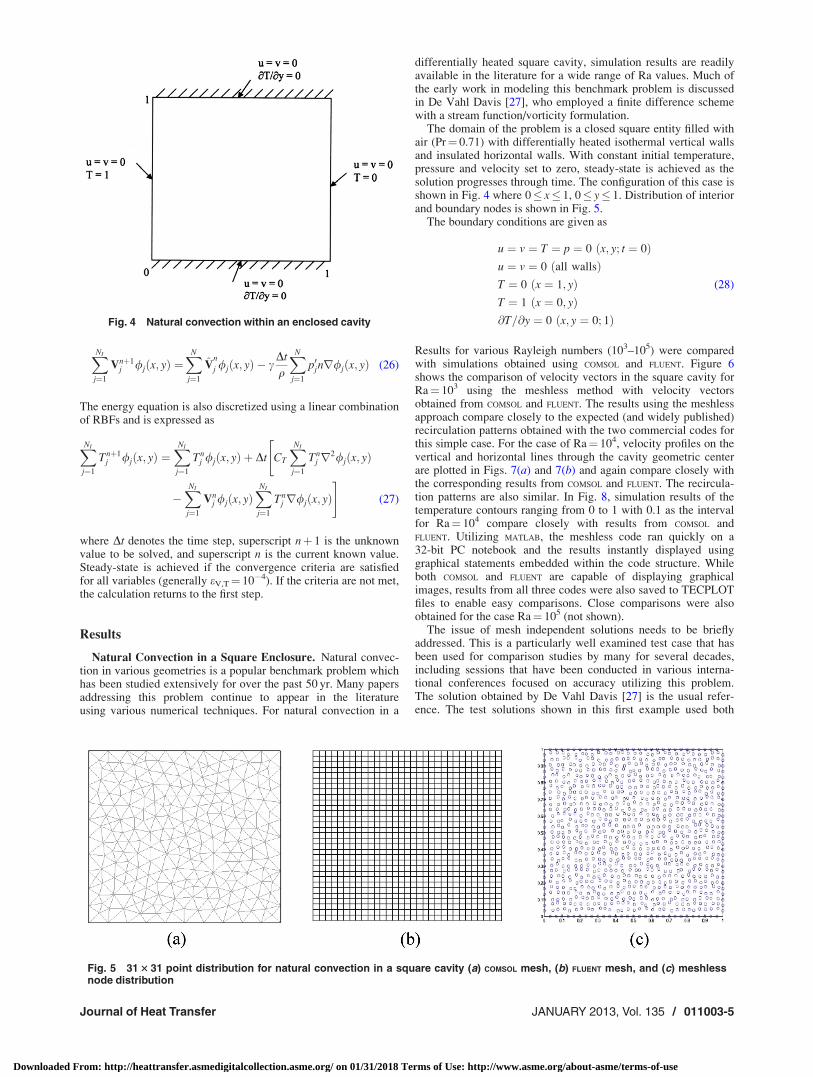
The domain of the problem is a closed square entity filled withair (Pr¼ 0.71) with differentially heated isothermal vertical wallsand insulated horizontal walls. With constant initial temperature,pressure and velocity set to zero, steady-state is achieved as thesolution progresses through time. The configuration of this case isshown in Fig. 4 where 0 x 1, 0 y 1. Distribution of interiorand boundary nodes is shown in Fig. 5.

The boundary conditions are given as

u ¼ v ¼ T ¼ p ¼ 0 x; y; t ¼ 0ð Þu ¼ v ¼ 0 all wallsð ÞT ¼ 0 x ¼ 1; yð ÞT ¼ 1 x ¼ 0; yð Þ@T=@y ¼ 0 x; y ¼ 0; 1ð Þ

(28)

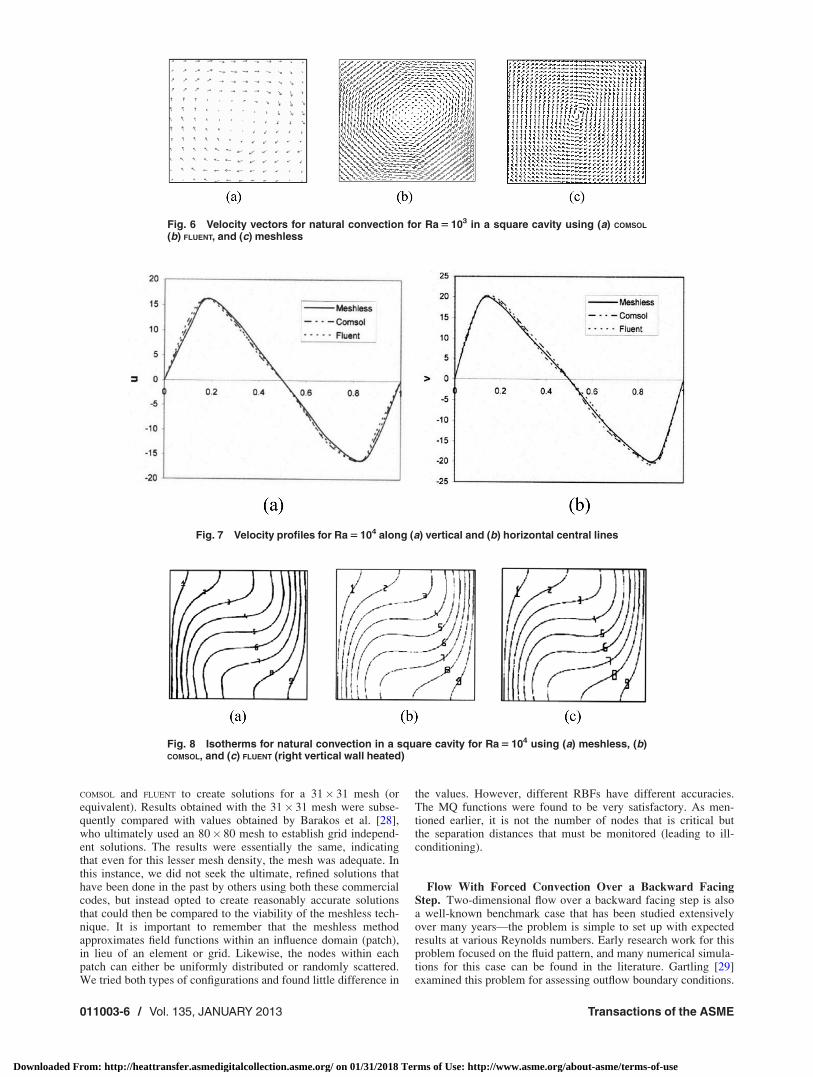
Results for various Rayleigh numbers (103–105) were comparedwith simulations obtained using COMSOL and FLUENT. Figure 6shows the comparison of velocity vectors in the square cavity forRa¼ 103 using the meshless method with velocity vectorsobtained from COMSOL and FLUENT. The results using the meshlessapproach compare closely to the expected (and widely published)recirculation patterns obtained with the two commercial codes forthis simple case. For the case of Ra¼ 104, velocity profiles on thevertical and horizontal lines through the cavity geometric centerare plotted in Figs. 7(a) and 7(b) and again compare closely withthe corresponding results from COMSOL and FLUENT. The recircula-tion patterns are also similar. In Fig. 8, simulation results of thetemperature contours ranging from 0 to 1 with 0.1 as the intervalfor Ra¼ 104 compare closely with results from COMSOL andFLUENT. Utilizing MATLAB, the meshless code ran quickly on a32-bit PC notebook and the results instantly displayed usinggraphical statements embedded within the code structure. Whileboth COMSOL and FLUENT are capable of displaying graphicalimages, results from all three codes were also saved to TECPLOTfiles to enable easy comparisons. Close comparisons were alsoobtained for the case Ra¼ 105 (not shown).

The issue of mesh independent solutions needs to be brieflyaddressed. This is a particularly well examined test case that hasbeen used for comparison studies by many for several decades,including sessions that have been conducted in various interna-tional conferences focused on accuracy utilizing this problem.The solution obtained by De Vahl Davis [27] is the usual refer-ence. The test solutions shown in this first example used both

Fig. 4 Natural convection within an enclosed cavity

Fig. 5 31 3 31 point distribution for natural convection in a square cavity (a) COMSOL mesh, (b) FLUENT mesh, and (c) meshlessnode distribution

Journal of Heat Transfer JANUARY 2013, Vol. 135 / 011003-5

Downloaded From: http://heattransfer.asmedigitalcollection.asme.org/ on 01/31/2018 Terms of Use: http://www.asme.org/about-asme/terms-of-use

COMSOL and FLUENT to create solutions for a 31� 31 mesh (orequivalent). Results obtained with the 31� 31 mesh were subse-quently compared with values obtained by Barakos et al. [28],who ultimately used an 80� 80 mesh to establish grid independ-ent solutions. The results were essentially the same, indicatingthat even for this lesser mesh density, the mesh was adequate. Inthis instance, we did not seek the ultimate, refined solutions thathave been done in the past by others using both these commercialcodes, but instead opted to create reasonably accurate solutionsthat could then be compared to the viability of the meshless tech-nique. It is important to remember that the meshless methodapproximates field functions within an influence domain (patch),in lieu of an element or grid. Likewise, the nodes within eachpatch can either be uniformly distributed or randomly scattered.We tried both types of configurations and found little difference in

the values. However, different RBFs have different accuracies.The MQ functions were found to be very satisfactory. As men-tioned earlier, it is not the number of nodes that is critical butthe separation distances that must be monitored (leading to ill-conditioning).

Flow With Forced Convection Over a Backward FacingStep. Two-dimensional flow over a backward facing step is alsoa well-known benchmark case that has been studied extensivelyover many years—the problem is simple to set up with expectedresults at various Reynolds numbers. Early research work for thisproblem focused on the fluid pattern, and many numerical simula-tions for this case can be found in the literature. Gartling [29]examined this problem for assessing outflow boundary conditions.

Fig. 7 Velocity profiles for Ra 5 104 along (a) vertical and (b) horizontal central lines

Fig. 6 Velocity vectors for natural convection for Ra 5 103 in a square cavity using (a) COMSOL

(b) FLUENT, and (c) meshless

Fig. 8 Isotherms for natural convection in a square cavity for Ra 5 104 using (a) meshless, (b)COMSOL, and (c) FLUENT (right vertical wall heated)

011003-6 / Vol. 135, JANUARY 2013 Transactions of the ASME

Downloaded From: http://heattransfer.asmedigitalcollection.asme.org/ on 01/31/2018 Terms of Use: http://www.asme.org/about-asme/terms-of-use

In 1992, Blackwell and Pepper [30] suggested flow over the back-ward facing step with heat transfer as an ASME benchmark testproblem. Numerical simulations from twelve different contribu-tors were presented.

The boundary conditions for this problem are described as

For Inlet Flow

u yð Þ ¼0; for 0 y 0:5

8y 1� 2yð Þ for 0:5 y 1

�vðyÞ ¼ 0

TðyÞ ¼ 1� 4y� 1ð Þ2h i

1� 1

54y� 1ð Þ2

� for 0 y 0:5

@TðyÞ@x¼ 0 for 0:5 y 1 (29)

On Upper and Lower Walls

u yð Þ ¼ vðyÞ ¼ 0

rT n ¼ 32

5

(30)

where n is the outward unit vector normal to the domainboundary.

For Outlet Flow

p ¼ 0 (31)

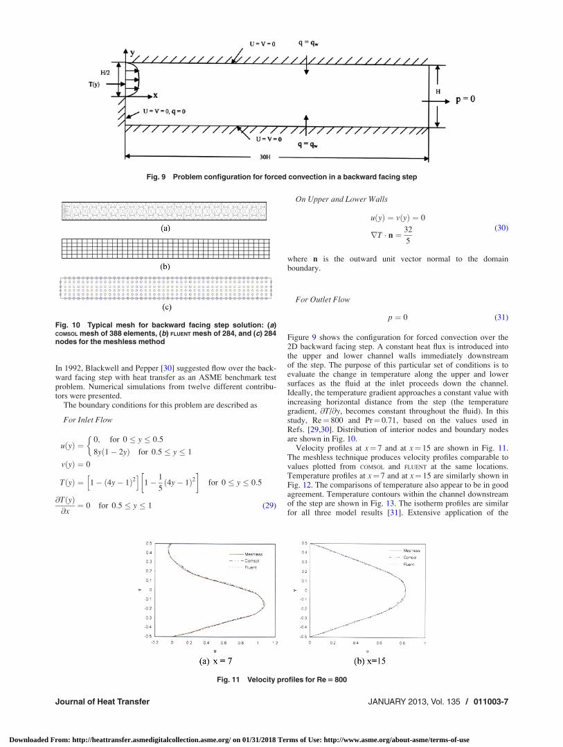
Figure 9 shows the configuration for forced convection over the2D backward facing step. A constant heat flux is introduced intothe upper and lower channel walls immediately downstreamof the step. The purpose of this particular set of conditions is toevaluate the change in temperature along the upper and lowersurfaces as the fluid at the inlet proceeds down the channel.Ideally, the temperature gradient approaches a constant value withincreasing horizontal distance from the step (the temperaturegradient, @T/@y, becomes constant throughout the fluid). In thisstudy, Re¼ 800 and Pr¼ 0.71, based on the values used inRefs. [29,30]. Distribution of interior nodes and boundary nodesare shown in Fig. 10.

Velocity profiles at x¼ 7 and at x¼ 15 are shown in Fig. 11.The meshless technique produces velocity profiles comparable tovalues plotted from COMSOL and FLUENT at the same locations.Temperature profiles at x¼ 7 and at x¼ 15 are similarly shown inFig. 12. The comparisons of temperature also appear to be in goodagreement. Temperature contours within the channel downstreamof the step are shown in Fig. 13. The isotherm profiles are similarfor all three model results [31]. Extensive application of the

Fig. 9 Problem configuration for forced convection in a backward facing step

Fig. 10 Typical mesh for backward facing step solution: (a)COMSOL mesh of 388 elements, (b) FLUENT mesh of 284, and (c) 284nodes for the meshless method

Fig. 11 Velocity profiles for Re 5 800

Journal of Heat Transfer JANUARY 2013, Vol. 135 / 011003-7

Downloaded From: http://heattransfer.asmedigitalcollection.asme.org/ on 01/31/2018 Terms of Use: http://www.asme.org/about-asme/terms-of-use

meshless method for more complex flow configurations can befound in Sarler et al. [22] and Zahab et al. [32].

Conclusions

The governing equations for transient fluid flow with convec-tive heat transfer are solved using RBFs. The use of RBFs allowsvelocity and temperature variables and their derivatives to beeasily established and solved with a general algorithm. To illus-trate the application of the technique, natural convection within asquare enclosure and forced convection over a backward facingstep are both solved. Results are compared with well-knownbenchmark solutions. Based upon the comparison studies, themeshless method using RBFs appears effective in simulating fluidflow with convection, and has the ability to be applied to a widerange of problems. The number of points required to obtain com-parable accuracy is less than mesh-based methods and a formalmesh structure is not required. The meshless method is an eco-nomical alternative for solving problems involving fluid flow withor without heat transfer.

Numerical implementation was done in MATLAB. Using a one-step pressure correction, the numerical algorithm needs only asmall number of calculations per iteration cycle. The overallnumerical procedure yields an algorithm that is fast and robust.Good agreement was achieved when comparing model resultsfrom COMSOL and FLUENT for these two simple convective heat trans-fer problems. Additional effort is underway to examine more com-plex and much larger problem domains, including 3D simulations,

over a wide class of problems. Recent results using the techniqueto model bioengineering flows and species transport, as well asenvironmental flows, appear promising.

Nomenclature

B ¼ 0; PrRaTCvis ¼ Pr; 1/ReCT ¼ 1; 1/Pe

c ¼ shape parameterg ¼ acceleration due to gravityL ¼ reference lengthN ¼ total number of nodes

NI ¼ number of internal nodesNIþ1 ¼ number of boundary nodes

n ¼ unit normal vectorp ¼ pressurep0 ¼ pressure correctionpo ¼ pressure at t¼ 0Pe ¼ Peclet number (Pe¼VL/a)Pr ¼ Prandtl number (Pr¼ �/a)Re ¼ Reynolds number (Re¼ qVL/l)Ra ¼ Rayleigh number (Ra¼ gb[Th�Tc]L

3/a�)rj ¼ radial dimension (x,y)rj ¼ radial basis function (vector)t ¼ time

T ¼ temperatureTc ¼ cold (or reference) temperatureTh ¼ hot temperature (heated wall)u ¼ horizontal (x) velocityv ¼ vertical (y) velocity

V ¼ velocity vectorVm ¼ iterated intermediate value of velocityV0 ¼ velocity correctionV̂ ¼ calculated velocity (not mass consistent)x ¼ spatial vector (x,y,z)x ¼ horizontal directiony ¼ vertical directiona ¼ thermal diffusivityb ¼ coefficient of thermal expansionc ¼ relaxation parameterC ¼ domain boundaryDt ¼ time stepeT ¼ error for temperature residualeV ¼ error for velocity residualh ¼ (T�T1)/(T2�T1) in 2D heat conduction testl ¼ dynamic viscosity� ¼ kinematic viscosityq ¼ density/ ¼ trial function

Fig. 12 Temperature profiles for Re 5 800

Fig. 13 Isotherms for backward step flow using (a) meshless,(b) COMSOL, and (c) FLUENT

011003-8 / Vol. 135, JANUARY 2013 Transactions of the ASME

Downloaded From: http://heattransfer.asmedigitalcollection.asme.org/ on 01/31/2018 Terms of Use: http://www.asme.org/about-asme/terms-of-use

X ¼ problem domainr ¼ gradient operatorr2 ¼ Laplacian operator

* ¼ denotes nondimensional

References[1] Atluri, S. N., and Shen, S., 2002, “The Meshless Local Petrov-Galerkin

(MLPG) Method: A Simple & Less-Costly Alternative to the Finite Elementand Boundary Element Methods,” Comput. Model. Eng. Sci., 3, pp. 11–52.

[2] Chen, W., 2002, “New RBF Collocation Schemes and Kernel RBFs WithApplications,” Lect. Notes Comput. Sci. Eng., 26, pp. 75–86.

[3] Kansa, E. J., 1990, “Multiquadrics—A Scattered Data Approximation SchemeWith Application to Computational Fluid Dynamics, Part I,” Comput. Math.With Appl., 19, pp. 127–145.

[4] Sarler, B., and Kuhn, G., 1999, “Primitive Variables Dual Reciprocity Bound-ary Element Method Solution of Incompressible Navier-Stokes Equations,”Eng. Anal. Boundary Elem., 23, pp. 443–455.

[5] Sarler, B., 2002, “Towards a Mesh-Free Computation of Transport Phenom-ena,” Eng. Anal. Boundary Elem., 26, pp. 731–738.

[6] Lin, H., and Atluri, S. N., 2001, “Meshless Local Petrov Galerkin Method(MLPG) for Convection-Diffusion Problems,” Comput. Model. Eng. Sci., 1, pp.45–60.

[7] Buhman, M. D., 2000, Radial Basis Functions, Cambridge University Press,Cambridge.

[8] Mai-Duy, N., and Tran-Cong, T., 2005, “An Efficient Indirect RBFN-BasedMethod for Numerical Solution of PDEs,” Numer. Methods Partial Differ.Equ., 21, pp. 770–790.

[9] Patankar, S. V., and Spalding, D. B., 1972, “Calculation Procedure for Heat,Mass and Momentum Transfer in Three-Dimensional Parabolic Flows,” Int. J.Heat Mass Transfer, 15(10), pp.1787–8061.

[10] Carrington, D. B., and Pepper, D. W., 2002, “Convective Heat Transfer Down-stream of a 3-D Backward-Facing Step,” Numer. Heat Transfer, Part A, 41(6–7),pp. 555–578.

[11] Wang, X., and Pepper, D. W., 2007, “Application of an hp-Adaptive FEM forSolving Thermal Flow Problems,” J. Thermophys. Heat Transfer, 21(1), pp.190–198.

[12] Carrington, D. B., Wang, X., and Pepper, D. W., 2010, “An h-Adaptive FiniteElement Method for Turbulent Heat Transfer,” Comput. Model. Eng. Sci.,61(1), pp. 23–44.

[13] Hardy, R. L., 1971, “Multiquadric Equations of Topography and Other IrregularSurfaces,” J. Geophys. Res., 76, pp. 1905–1915.

[14] Franke, R., 1979, “A Critical Comparison of Some Methods for Interpolation ofScattered Data,” Naval Postgraduate School, Report No. TR NPS-53-79-003.

[15] Franke, C., and Schaback, R., 1998, “Solving Partial Differential EquationsUsing Radial Basis Functions,” Appl. Math. Comput., 3, pp. 73–82.

[16] Fasshauer, G. E., 2007, Meshfree Approximation Methods With MATLAB (Volume 6of Interdisciplinary Mathematical Sciences), World Scientific Pub. Co., Singapore.

[17] Atluri, S. N., and Zhu, T., 1998, “A New Mesh-Less Local Petrov-GalerkinApproach in Computational Mechanics,” Comput. Mech., 22, pp. 117–127.

[18] Balachandran, G. R., Rajagopal, A., and Sivakumar, S. M., 2008, “Mesh FreeGalerkin Method Based on Natural Neighbors and Conformal Mapping,” Com-put. Mech., 42(6), pp. 885–905.

[19] Bern, M., and Eppstein, D., 1992, “Mesh Generation and Optimal Triangu-lation,” Computing in Euclidean Geometry, Vol. 1, D. Z. Du and F. K. Hwang,eds., World Scientific Publishing Co., Singapore, pp. 23–90.

[20] Choi, Y., and Kim, S. J., 1999, “Node Generation Scheme for the Mesh-LessMethod by Voronoi Diagram and Weighted Bubble Packing,” 5th US NationalCongress on Computational Mechanics, Boulder, CO.

[21] Li, X. Y., Teng, S. H., and Ungor, A., 2000, “Point Placement for MeshlessMethods Using Sphere Packing and Advancing Front Methods,” ICCES’00,Los Angeles, CA.

[22] Sarler, B., Lorbiecka, A. Z., and Vertnik, R., 2010, “Heat and Mass TransferProblems in Continuous Casting of Steel: Multiscale Solution by MeshlessMethod,” International Conference on Fluid Dynamics, Cairo, Egypt, Dec.16–19, Vol. 10.

[23] Gewali, L., and Pepper, D. W., 2010, “Adaptive Node Placement for Mesh-FreeMethods,” ICCES 10, Las Vegas, NV, Mar. 28–Apr. 1.

[24] Incropera, F. P., and DeWitt, D. P., 2002, Fundamentals of Heat and MassTransfer, 5th ed., J. Wiley & Sons, New York.

[25] Pepper, D. W., 2010, “Meshless Methods for PDEs,” Scholarpedia, 5(5), p. 9838.[26] Spalding, D. B., 1985, “Numerical Simulation of Natural Convection in Porous

Media,” Conference on Natural Convection: Fundamentals and Applications,Hemisphere, Washington, DC, pp. 655–673.

[27] De Vahl Davis, G., 1983, “Natural Convection of Air in a Square Cavity: ABench Mark Numerical Solution,” Int. J. Numer. Methods Fluids, 3, pp.249–264.

[28] Barakos, G., Mitsoulis, E., and Assimacopoulos, D., 1994, “Natural ConvectionFlow in a Square Cavity Revisited: Laminar and Turbulent Models With WallFunctions,” Int. J. Numer. Methods Fluids, 18, pp. 695–719.

[29] Gartling, D. K., 1990, “A Test Problem for Outflow Boundary Conditions—Flow Over a Backward-Facing Step,” Int. J. Numer. Methods Fluids, 11, pp.953–967.

[30] Blackwell, B. F., and Pepper, D. W., 1992, “Benchmark Problems for HeatTransfer Codes,” ASME Winter Annual Meeting (HTD), 21, pp. 190–198.

[31] Kalla, N. K., 2007, “Solution of Heat Transfer and Fluid Flow Problems UsingMeshless Radial Basis Function Method,” M.S. thesis, UNLV, Las Vegas, NV.

[32] Zahab, Z. E., Divo, E., and Kassab, A. J., 2009, “A Localized CollocationMeshless Method (LCMM) for Incompressible Flows CFD Modeling WithApplications to Transient Hemodynamics,” Eng. Anal. Boundary Elem., 33, pp.1045–1061.

Journal of Heat Transfer JANUARY 2013, Vol. 135 / 011003-9

Downloaded From: http://heattransfer.asmedigitalcollection.asme.org/ on 01/31/2018 Terms of Use: http://www.asme.org/about-asme/terms-of-use