ORIGINAL PAPER

A mechanistic model of heat transfer for gas–liquid flowin vertical wellbore annuli

Bang-Tang Yin1• Xiang-Fang Li2 • Gang Liu1

Received: 20 July 2016 / Published online: 27 October 2017

� The Author(s) 2017. This article is an open access publication

Abstract The most prominent aspect of multiphase flow is

the variation in the physical distribution of the phases in the

flow conduit known as the flow pattern. Several different

flow patterns can exist under different flow conditions which

have significant effects on liquid holdup, pressure gradient

and heat transfer. Gas–liquid two-phase flow in an annulus

can be found in a variety of practical situations. In high rate

oil and gas production, it may be beneficial to flow fluids

vertically through the annulus configuration between well

tubing and casing. The flow patterns in annuli are different

from pipe flow. There are both casing and tubing liquid films

in slug flow and annular flow in the annulus. Multiphase

heat transfer depends on the hydrodynamic behavior of the

flow. There are very limited research results that can be

found in the open literature for multiphase heat transfer in

wellbore annuli. A mechanistic model of multiphase heat

transfer is developed for different flow patterns of upward

gas–liquid flow in vertical annuli. The required local flow

parameters are predicted by use of the hydraulic model of

steady-state multiphase flow in wellbore annuli recently

developed by Yin et al. The modified heat-transfer model

for single gas or liquid flow is verified by comparison with

Manabe’s experimental results. For different flow patterns, it

is compared with modified unified Zhang et al. model based

on representative diameters.

Keywords Gas–liquid flow � Vertical annuli � Heattransfer � Tubing liquid film � Casing liquid film

1 Introduction

As oil and gas development moves from land or shallow

water to deep and ultradeep waters, multiphase flow occurs

during production and transportation (Chen 2011). The

flow normally occurs in horizontal, inclined, or vertical

pipes and wells. Gas–liquid two-phase flow in an annulus

can be found in a variety of practical situations. In high rate

oil and gas production, it may be beneficial to flow fluids

vertically through the annulus configuration between well

tubing and casing. For surface facilities, some large, under-

utilized flow lines can be converted to dual-service by

putting a second pipe through the large line (i.e., flowing

produced water in the inner line and gas in the annulus).

During gas production, liquids may accumulate at the

bottom of the gas wells during their later life. In order to

remove or ‘‘unload’’ the undesirable liquids, a siphon tube

is often installed inside the tubing string, which would form

a gas–liquid two-phase flow in the annulus. Flow-assurance

problems, such as hydrate blocking (Jamaluddin et al.

1991; Li et al. 2013; Wang et al. 2014, 2016) and wax

deposition (Zhang et al. 2013; Bryan 2016; Theyab and

Diaz 2016), are strongly associated with both the hydraulic

and thermal behavior. For example, they are related to the

fluid velocity, liquid fraction, slug characteristics, pressure

gradient and convective-heat-transfer coefficients of dif-

ferent phase and flow patterns in multiphase flow. There-

fore, multiphase hydrodynamics and heat transfer in an

annulus need to be modeled properly to guide the design

and operation of flow systems.

& Bang-Tang Yin

yinbangtang@163.com

1 School of Petroleum Engineering, China University of

Petroleum (East China), Qingdao 266580, Shandong, China

2 College of Petroleum Engineering, China University of

Petroleum, Beijing 102249, China

Edited by Yan-Hua Sun

123

Pet. Sci. (2018) 15:135–145

https://doi.org/10.1007/s12182-017-0193-y

Compared to theoretical studies of multiphase hydro-

dynamics (Liu et al. 2007; Wang and Sun 2009), and

multiphase heat transfer in pipe flow (Zheng et al. 2016;

Gao et al. 2016; Karimi and Boostani 2016; Rushd and

Sanders 2017), there are very limited research results in the

open literature for multiphase heat transfer in wellbore

annuli. Davis et al. (1979) obtained a model for calculating

the local Nusselt numbers of stratified gas/liquid flow in

turbulent liquid/turbulent gas conditions. The model was

tested with heat-transfer experiments for air/water flow in a

63.5-mm inside diameter (ID) tube. Guo et al. (2017)

established a mathematical model of heat transfer in a gas-

drilling system, considering the flowing gas, formation

fluid influx, Joule–Thomson cooling and entrained cuttings

in the annular space. However, the multiphase flow effect

on the heat transfer was not considered.

Shoham, et al. (1982) undertook experiments on heat-

transfer for slug flow in a horizontal pipe. He found a

substantial difference in heat-transfer coefficient existed

between the top and bottom of the slug. Developing heat-

transfer correlations of different flow patterns was the aim

of most previous studies (Shah 1981). Twenty heat-transfer

correlations were compared in Kim’s study (Kim et al.

1997). He collected the experimental data from the open

literature and recommended the correlations for different

flow patterns. However, the errors with the experimental

results by Matzain (1999) were large. Later, a compre-

hensive mechanistic model about heat transfer in gas–liq-

uid pipe flow was obtained (Manabe 2001). It was

compared with the experimental data, and the performance

was better. However, there were some inconsistencies in

annular and slug flow. It needed to be modified.

Zhang et al. (2006) developed a unified model of multi-

phase heat transfer for different flow patterns of gas–liquid

pipe flow at all inclinations – 90� to ? 90� from the hori-

zontal. The required local flow parameters were predicted by

use of the unified hydrodynamic model for gas/liquid pipe

flow developed by Zhang et al. (2003a, b). However, it is not

fit for the gas–liquid flow in an annulus, because the flow

patterns in annuli are different from pipe flow patterns, as

seen in Fig. 1 (Caetano 1986). A new heat-transfer model

for gas–liquid flow in vertical annuli needs to be established.

A hydraulic model was developed to predict flow pat-

terns, liquid holdup and pressure gradients for steady-state

gas–liquid flow in wellbore annuli (Yin et al. 2014). The

major advantage of this model compared with previous

mechanistic models is that it is developed based on the

dynamics of slug flow, and the liquid-film zone is used as

the control volume. The effects of the tubing liquid film,

casing liquid film and the droplets in the gas core area on the

mass and momentum transfers are considered. Multiphase

heat transfer depends on the hydrodynamic behavior of the

flow. The objective of this study is to develop a heat-transfer

model for gas–liquid flow that is consistent with the

hydrodynamic model in vertical wellbore annuli.

2 Modeling

2.1 Single-phase flow

When fluids flow through an annulus, the surrounding

temperature is cold, heat is lost from the fluids to the for-

mation, resulting in a decline in temperature, as seen in

Bubblyflow

Dispersed-bubble flow

BackFrontSlug flow

Churnflow

Annularflow

Fig. 1 Flow patterns for upward vertical flow in an annulus (Caetano

1986)

v1

q1

h1(l+dl )

h1(dl )

Fig. 2 Heat transfer from the annulus to the formation

136 Pet. Sci. (2018) 15:135–145

123

Fig. 2. In the steady state, there is no heat loss from the

annulus to the tube. For the fluids in the annulus, the

conservation of mass is:

d

dlqlvlð Þ ¼ 0 ð1Þ

where ql is the density of liquids, kg/cm3; vl is the velocity

of liquids in the annulus, m/s; dl is the length of the element.

The conservation of momentum is:

d

dlqlv

2l

� �¼ � dp

dl� qlg sin h�

spdA

ð2Þ

where p is the unit pressure, MPa; g is the gravity accel-

eration, m/s2; h is the inclination angle, �; s is the friction;

d is the annulus diameter, m; A is the cross area of the

annulus, m2.

The energy equation is:

d

dlqlvl eþ 1

2v2l

� �� �¼ � d

dlpvlð Þ � qlvlg sin h�

q1

Að3Þ

where e is the internal energy of the unit, J/kg; q1 is the

heat loss from the annulus to the formation, W.

Using the mass balance, we can reduce Eqs. (2) and (3)

further:

dp

dl¼ �qlvl

dvl

dl� qlg sin h�

spdA

ð4Þ

qlvld

dleþ p

ql

� �¼ �qlvl

dvl

dl� qlvlg sin h�

q1

Að5Þ

Or

dh

dl¼ �vl

dvl

dl� g sin h� q1

Aqlvl¼ �vl

dvl

dl� g sin h� q1

w1

ð6Þ

where h is the enthalpy, J/kg; wl is the mass flow rate of

liquids in the annulus, kg/s.

Using the definition of the dimensionless temperature

TD proposed by Hasan and Kabir (1991), we may write an

expression for heat transfer from the wellbore/formation

interface to the formation as

q1 ¼2pke Twb � Teð Þ

TDð7Þ

where Te is the formation temperature, �C; Twb is the

wellbore temperature, �C; ke is the conductivity of forma-

tion, W/(m �C); the dimensionless temperature, defined by

Hasan and Kabir (1991), TD, can be easily estimated from

the following models.

TD¼1:1281

ffiffiffiffiffitD

p1�0:3

ffiffiffiffiffitD

pð Þ; 10�10�tD�1:5

0:4063þ0:5lntDð Þ 1þ0:6

tD

� �; tD[1:5

8<

:

where tD is the dimensionless flowing time,

tD ¼ t

r2w

where t is the flowing time, s; rw is the wellbore radius, m.

The heat transfer from the annulus to the well wall, q1may be expressed in terms of an overall heat coefficient

(Hansan and Kabir 1994),

q1 ¼ 2prcoUa Ta � Twbð Þ ð8Þ

where rco is the outside casing radius, m; Ta is the fluid

temperature in the annulus, �C; Ua is the overall heat-

transfer coefficient of the annulus, W/(m2 �C).

1

Ua

¼ rco

rcihaþ rco ln rco=rcið Þ

kcasþ rco ln rw=rcoð Þ

kcemð9Þ

where rci is the inside casing radius, m; ha is the convec-

tive-heat-transfer coefficient of fluids in the annulus, W/

(m2 �C); kcas is the conductivity of the casing wall, W/(m

�C); kcem is the conductivity of cement, W/(m �C).Combining Eqs. (7) and (8) gives,

q1 ¼2pke Twb � Teð Þ

TD¼ 2prcoUa Ta � Twbð Þ

q1 ¼wlcp

A0 Ta � Teð Þ ð10Þ

where cp is the fluid heat capacity at the constant pressure

in the annulus, J/(kg �C).

A0 ¼ w1cp

2pke þ rcoUaTD

rcoUake

� �

where A0 is the local parameter defined in Eq. (10).

Combining Eqs. (6), (8) and (10) yields,

dh

dl¼ �vl

dvl

dl� g sin h� cp

A0 Ta � Teð Þ ð11Þ

The enthalpy gradient can be written in terms of the

temperature and pressure gradients:

dh

dl¼ cp

dT

dl� glcp

dp

dlð12Þ

where gl is the fluid Joule–Thomson coefficient in the

annulus, �C/MPa.

Combining Eqs. (11) and (12) gives

dTa

dlþ 1

A0 Ta � Teð Þ þ 1

cpvldvl

dlþ g sin h� glcp

dp

dl

� �¼ 0

ð13Þ

Defining a dimensionless parameter Ua, as

Ua ¼ qlvldvl

dlþ qlg sin h� qlglcp

dp

dl

� �dp

dl

We can write Eq. (13) as

Pet. Sci. (2018) 15:135–145 137

123

dTa

dlþ 1

A0 Ta � Teð Þ þ 1

qlcp

dp

dlUa ¼ 0 ð14Þ

Equation (14) is the energy conservation equation of

fluids in the annulus.

We can write Eq. (14) as

dTa

dlþ 1

A0 Ta ¼1

A0 Te �1

qlcp

dp

dlUa ð15Þ

Up to this point, only mathematical manipulations have

been done to the enthalpy equation, and the analysis has

been carried out rigorously without simplification. Now if

Eq. (15) is used for an onshore production well, then

assuming the surrounding formation temperature is a linear

function of depth, it can be expressed as

Te ¼ Tei � geL sin h ð16Þ

where Tei is the temperature of formation at wellbore

intake, �C; ge is the formation thermal gradient, �C/100 m;

L is the depth, m.

If Eq. (15) is used for the riser of an offshore production

well, then the surrounding sea temperature is not a linear

function of depth. It will be calculated according to the

actual environment (Wang and Sun 2009).

If, for a certain segment of the wellbore, Ua, cp, gl, ge, h,vldvl/dl and dp/dl can be approximately constants, com-

bining Eqs. (15) and (16) and integrating, yields an explicit

equation for the temperature:

Ta ¼ Tei � geL sin hð Þ þ Ti � Teið Þ exp �L=A0ð Þ þ geA0 sin h

� 1� exp �L=A0ð Þ½ � þ 1

qcp

dp

dL

UA0 1� exp �L=A0ð Þ½ �

ð17Þ

2.2 Bubbly flow and dispersed-bubble flow

In bubbly flow and dispersed-bubble flow, the gas holdup is

small and the gas superficial velocity is low, the gas phase

is distributed as small discrete bubbles in a continuous

liquid phase. So bubbly flow and dispersed-bubble flow can

be treated as pseudo-single-phase flow. The fluid physical

properties are adjusted based on the liquid holdup. Zhang

et al. correction (2006) for bubbly flow will be modified

based on ‘‘hydraulic diameter’’.

dR ¼ dci � dtuo ð17Þ

where dR is the hydraulic diameter, m; dci is the inside

diameter of casing,m;dtuo is the outside diameter of tubing,m.

Then the convective-heat-transfer coefficient of Eq. (9)

for bubbly or dispersed-bubbly flow is obtained from

hab ¼NmNukm

dRð18Þ

where km is the conductivity of the mixture, W/(m �C),

km ¼ 1� Hlð Þkg þ Hlkl

where Hl is the liquid hold up; kl is the conductivity of

liquid, W/(m �C); kg is the conductivity of gas, W/(m �C).NmNu is the mixture Nusselt number (Zhang et al. 2006).

NmNu ¼

fm2

� �NmReN

mPr

1:07þ 12:7ffiffiffiffifm2

qNm2=3

Pr � 1� �

lllm

� �ð19Þ

where fm is the friction factor of the mixture; ll is the

viscosity of liquid, mPa s; lm is the viscosity of the mix-

ture, mPa s; lg is the viscosity of gas, mPa s,

lm ¼ 1� Hlð Þlg þ Hlll

NmRe and Nm

Pr is the Reynolds number and Prandtl number

of the mixture.

NmRe ¼

qmvmdRlm

NmPr ¼

cpmlmkm

where qm is the density of the mixture, kg/m3; vm is the

velocity of the mixture, m/s; cpm is the specific heat of the

mixture, J/(kg �C),

cpm ¼ 1� Hlð Þcpg þ Hlcpl

where cpl is the specific heat of liquid, J/(kg �C); cpg is thespecific heat of gas, J/(kg �C).

So the associated parameters will be modified,

1

Uab

¼ rco

rcihabþ rco ln rco=rcið Þ

kcasþ rco ln rw=rcoð Þ

kcem

A0b ¼

wmcpm

2pke þ rcoUabTD

rcoUabke

� �

Uab ¼ qmvmdvm

dlþ qmg sin h� qmgmcpm

dp

dl

� �dp

dl

where the subscript b represents in bubble flow or dis-

persed-bubble flow; the subscript m represents the mixture

properties of gas and liquid, A0b is the local parameter

defined in Eq. (20).

Equation (15) can be written as

dTa

dlþ 1

A0b

Ta ¼1

A0b

Te �1

qmcpm

dp

dlUab ð20Þ

Then Eq. (20) can be used in the heat transfer in bubble

flow and dispersed-bubble flow based on the modified

convective-heat-transfer coefficient hab.

2.3 Annular flow

As shown in Fig. 3, there are tubing and casing films in

annular flow in annuli, which is different from the annular

138 Pet. Sci. (2018) 15:135–145

123

flow in pipes. Assume there are no temperature and heat-

transfer exchanges in the vertical direction. The tempera-

ture and heat changes are only caused by the heat transfer

in the radial direction. Heat distribution in annuli includes

three parts: in casing film, tubing film and gas core. The

heat-transfer models in annuli are obtained by a method

similar to that above.

For the gas core, the energy conservation equation is as

follows,

dTgc

dlþ 1

A0gc

Tgc � Tcf� �

� 1

B0gc

Ttuf � Tgc� �

þ 1

qgccpgc

dp

dlUgc

¼ 0

ð21Þ

where Tgc is the temperature of the gas core, �C; Tcf is thetemperature of the casing film, �C; Ttuf is the temperature

of the tubing film, �C; cpgc is the specific heat of the gas

core, J/(kg �C); A0gc, B0

gc, Ugc are the local parameters

defined as follows:

A0gc ¼

wgccpgc

2p rci � dcð ÞUgc

B0gc ¼

wgccpgc

2p rtuo þ dtuð ÞUtuf

Ugc ¼ qgcvgcdvgc

dlþ qgcg sin h� qgcggccpgc

dp

dl

� �dp

dl

where wgc is the mass flow rate of the gas core, kg/s; cpgc is

the specific heat of the gas core, J/(kg �C); vgc is the

velocity of the gas core, m/s; qgc is the density of the gas

core, kg/m3; ggc is the Joule–Thomson coefficient of the

gas core, �C/MPa; Ugc is the overall heat-transfer coeffi-

cient of the gas core, W/(m2 �C), and defined as

1

Ugc

¼ rci � dcrtuo þ dtuð Þhgc

where rtuo is the outside radius of the tubing, m; dtu is thethickness of the tubing film, m; dc is the thickness of the

casing film, m; hgc is the convective-heat-transfer coeffi-

cient of the gas core, W/(m2 �C).Utuf is the overall heat-transfer coefficient of the tubing

film, W/(m2 �C), and defined as

1

Utuf

¼ rtuo þ dturtuohtuf

þ rtuo þ dtuð Þ ln rtuo þ dtuð Þ=rtuoð Þktu

where htuf is the convective-heat-transfer coefficient of the

tubing film, W/(m2 �C); ktu is the conductivity of the tubingwall, W/(m �C).

For the tubing film, the energy conservation equation is

as follows,

dTtuf

dlþ wgccpgc

wtufcptufB0gc

Ttuf � Tgc� �

þ 1

qtufcptuf

dp

dlUtuf ¼ 0

ð22Þ

where wtuf is the mass flow rate of the liquid tubing film,

kg/s; qtuf is the density of the liquid tubing film, kg/m3;

cptuf is the specific heat of the liquid tubing film, J/(kg �C);Utuf is the local constant and defined as follows:

Utuf ¼ qtufvtufdvtuf

dlþ qtufg sin h� qtufgtufcptuf

dp

dl

� �dp

dl

where vtuf is the velocity of the liquid tubing film, m/s; gtufis the Joule–Thomson coefficient of the liquid tubing film,

�C/MPa.

For the casing film, the energy conservation equation is

as follows,

dTcf

dlþ 1

C0cf

Tcf � Teð Þ � wgccpgc

wcfcpcfA0gc

Tgc � Tcf� �

þ 1

qcfcpcf

dp

dlUcf

¼ 0 ð23Þ

where wcf is the mass flow rate of liquid casing film, kg/s;

qcf is the density of liquid casing film, kg/m3; cpcf is the

specific heat of liquid casing film, J/(kg �C); C0cf is the local

parameter defined in Eq. (23),

C0cf ¼

wcfcpcf

2pke þ rcoUcfTD

rcoUcfke

� �

Htuf(l+dl ) Hgc(l+dl )Hcf(l+dl )

qtufc

qccf

qcff

Hcf(l )

Hgc(l )Htuf(l )Tubing liquidfilm

Casing liquidfilm

Fig. 3 Control volume and temperatures in annular flow (qtufc is the

heat transfer from the tubing film to the gas core, W; qccf is the heat

transfer from the gas core to the casing film, W; qcff is the heat

transfer from the casing film to the formation, W)

Pet. Sci. (2018) 15:135–145 139

123

Ucf is the overall heat-transfer coefficient of casing film,

W/(m2 �C), and defined as

1

Ucf

¼ rci

rci � dcð Þhcfþ rco ln rco=rcið Þ

kcasþ rco ln rw=rcoð Þ

kcem

where hcf is the convective-heat-transfer coefficient of

casing film, W/(m2 �C).Ucf is the local parameter defined in Eq. (23),

Ucf ¼ qcfvcfdvcf

dlþ qcfg sin h� qcfgcfcpcf

dp

dl

� �dp

dl

where vcf is the velocity of the liquid casing film, m/s; gcf isthe Joule–Thomson coefficient of the liquid casing film,

�C/MPa.

Equations (21)–(23) are the heat-transfer models for

gas–liquid annular flow in annuli. Then the fluid temper-

ature in the wellbore is calculated by a weighted average

method based on holdup.

Tta ¼ HtufTtuf þ 1� Htuf � Hcfð ÞTgc þ HcfTcf ð24Þ

where Htuf is the holdup of the liquid tubing film; Hcf is the

holdup of the liquid casing film.

The convective-heat-transfer coefficients for the casing

film, the tubing film and gas core are obtained by the fol-

lowing equations

htuf ¼N tufNuklf

dtufR; hgc ¼

NgcNukgc

dgcR; hcf ¼

NcfNuklf

dcfR

where klf, kgc are the thermal conductivities of the liquid

film and gas core, W/(m �C); dtufR, dcfR, dgcR are the

‘‘hydraulic diameter’’ of the tubing film, the casing film

and gas core, m.

dtufR ¼ rtuo þ dtuð Þ � rtuo ¼ dtudcfR ¼ rci � rci � dcð Þ ¼ dcdgcR ¼ rci � dcð Þ � rtuo þ dtuð Þ

The Nusselt numbers for the liquid film and gas core are

calculated by using the correlations for single-phase con-

vective heat transfer. The Petukhov correlation (1970) is

used for turbulent liquid-film flow:

N ifNu ¼

fif2

� �N ifReN

ifPr

1:07þ 12:7ffiffiffifif2

qN ifPrð Þ2=3�1

�lllm

� �0:25

ð25Þ

where i is tubing film or casing film, i = tu or c. fif is the

friction factor at the wall in contact with the liquid film.

N ifRe ¼

qlvifdifRll

N ifPr ¼

cpllifRkl

The Dittus and Boelter correlation (1985) is used for

turbulent gas core flow,

NgcNu ¼ 0:023 N

gcReð Þ0:8 N

gcPrð Þ0:33 ð26Þ

For fully developed laminar flows of the liquid film and

gas core, the Nusselt number approaches a constant value.

According to Zhang et al. (2006), the Nusselt numbers for

fully developed laminar flows are calculated by,

N ifNu ¼ 3:657þ 7:541� 3:657

0:50:5� di

2ffiffiffiffiffiffiffiffiffiffiffiffiffiffiffiffiffir2ci � r2tuo

p

!

ð27Þ

NgcNu ¼ 3:657 ð28Þ

The associated hydraulic parameters are calculated by the

Yin et al. model (Yin et al. 2014), such as the thickness of

the liquid film, dc and dtu, the hold up, liquid and gas

physical properties .

2.4 Slug flow

2.4.1 Film region

The flow characters of the film region are similar to the

annular flow. The difference is that the gas core with liquid

droplets changes into the Taylor bubble. So, the overall

heat-transfer coefficients of Eqs. (21) and (23) should

change from Ugc to UT. Then the heat transfer of the film

region can be calculated.1

UT

¼ 1

hTð29Þ

where UT is the overall heat-transfer coefficient of the

Taylor bubble, W/(m2 �C); hT is the convective-heat-

transfer coefficient of the Taylor bubble, W/(m2 �C).

hT ¼ NTNukT

dTRð30Þ

where kT is the thermal conductivities of the Taylor bubble,

W/(m �C); dTR is the ‘‘representative diameter’’ of the

Taylor bubble.

dTR ¼ 2

ffiffiffiffiffiffiffiffiffiffiffiffiffiffiffiffiffiffiffiffiffiffiffiffiffiffiffiffiffiffiffiffiffiffiffiffiffiffiffiffiffiffiffiffiffiffiffirci � dcð Þ2� rtuo þ dtuð Þ2

q

2.4.2 Slug region

There are small discrete bubbles in a continuous liquid

phase. The flow characters are similar to bubbly flow. So,

the heat transfer can be calculated by the bubbly flow model.

2.4.3 Slug unit

The fluid temperature in the wellbore is calculated by the

weighted average method based on holdup.

Ts ¼HtufTtuf þ 1�Htuf �Hcfð ÞTTþHcfTcf½ �lFþTlsls

lUð31Þ

where Ts is the temperature of the fluid in slug flow, �C; Tlsis the temperature of the fluid in the slug unit, �C; TT is the

140 Pet. Sci. (2018) 15:135–145

123

temperature of the Taylor bubble, �C; lF is the length of the

liquid film, m; ls is the length of the slug unit, m; lU is the

length of the whole slug, m.

3 Solution procedure

Figure 4 shows the overall solution flowchart for the present

model. First, the parameters of fluid properties are provided.

Then the flow pattern is determined based on the input

variables and then all the flow conditions, such as flow

pattern, liquid holdups, local fluid velocities of the liquid

film and gas core, and slug characteristics, are predicted by

use of the hydraulic model of steady-state multiphase flow in

wellbore annuli recently developed by Yin et al. (2014).

Based on flow patterns, further calculations are performed

in different subroutines. If the flow pattern is single-phase

flow, single-phase heat-transfer calculation will be performed;

if the flow pattern is bubble or dispersed-bubble flow, the

corresponding hydraulic model and heat-transfer model will

be called for calculation. For annular flow, corresponding

hydraulic and heat-transfer calculations will be made. For

slug flow, corresponding hydraulic and heat-transfer calcu-

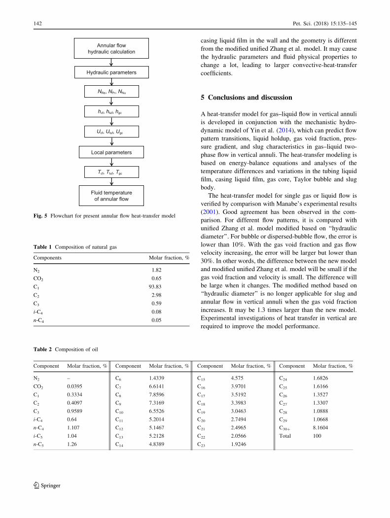
lations will be made, as seen in Fig. 4. Figure 5 is the

flowchart for the present annular flow heat-transfer model.

4 Comparisons with the unified Zhang model

The heat transfer of single-phase gas or liquid flow can be

calculated by the present model if the thermal conductivity

of the tubing wall is infinite. The composition of simulated

fluids is shown in Tables 1 and 2. The simulated annulus

outer diameter is 76.2 mm, and the inner diameter is

42.2 mm. The basic parameters are shown in Table 3.

Figures 6 and 7 show comparisons between the simu-

lations of new models and experimental measurements

(Manabe 2001) of the convective-heat-transfer coefficients

for single-phase gas and liquid flows, respectively. The

good agreement between the simulations and experimental

measurements for single-phase gas and liquid flows indi-

cates that the new models are reliable and the selected

correlations are appropriate.

There are few experimental research results in the open

literature for multiphase heat transfer in annuli. The unified

Zhang et al. model (2006) is verified by comparison with

Manabe’s experimental results for different flow patterns in

a crude-oil/natural gas system, and good agreement has

been observed in the comparison. So, the unified Zhang

et al. model is modified to calculate the heat transfer of

gas–liquid flow in annuli based on the ‘‘hydraulic diame-

ter’’ of the annuli, Eq. (17), and the results are compared

with the present mechanistic heat-transfer model for gas–

liquid flow in annuli.

Figures 8, 9, and 10 are comparisons of convective-

heat-transfer coefficient for bubble flow, annular flow and

slug flow predicted by the present model and the modified

unified Zhang et al. model (2006). For the bubble flow, the

data points are located inside the 10% error band. The

agreement is good. It shows that the influence of annulus

geometry is small for the low gas volume fraction. For the

annular and slug flow in annuli, most of the data points are

located inside the 30% error band and all are overesti-

mated. It may because there is a tubing liquid film and a

Input the fluid and flowing parameters

Single phase gas or liquid

Bubble flow

Annular flow

Slug flow calculation

Single phasehydraulic calculation

Bubble flowhydraulic calculation

Annular flowhydraulic calculation

Slug flow heattransfer

Yes

No

Yes

Yes

No

No

Single phaseheat transfer

Bubble flowheat transfer

Annular flowheat transfer

Output

Fig. 4 Overall flowchart for present model

Pet. Sci. (2018) 15:135–145 141

123

casing liquid film in the wall and the geometry is different

from the modified unified Zhang et al. model. It may cause

the hydraulic parameters and fluid physical properties to

change a lot, leading to larger convective-heat-transfer

coefficients.

5 Conclusions and discussion

A heat-transfer model for gas–liquid flow in vertical annuli

is developed in conjunction with the mechanistic hydro-

dynamic model of Yin et al. (2014), which can predict flow

pattern transitions, liquid holdup, gas void fraction, pres-

sure gradient, and slug characteristics in gas–liquid two-

phase flow in vertical annuli. The heat-transfer modeling is

based on energy-balance equations and analyses of the

temperature differences and variations in the tubing liquid

film, casing liquid film, gas core, Taylor bubble and slug

body.

The heat-transfer model for single gas or liquid flow is

verified by comparison with Manabe’s experimental results

(2001). Good agreement has been observed in the com-

parison. For different flow patterns, it is compared with

unified Zhang et al. model modified based on ‘‘hydraulic

diameter’’. For bubble or dispersed-bubble flow, the error is

lower than 10%. With the gas void fraction and gas flow

velocity increasing, the error will be larger but lower than

30%. In other words, the difference between the new model

and modified unified Zhang et al. model will be small if the

gas void fraction and velocity is small. The difference will

be large when it changes. The modified method based on

‘‘hydraulic diameter’’ is no longer applicable for slug and

annular flow in vertical annuli when the gas void fraction

increases. It may be 1.3 times larger than the new model.

Experimental investigations of heat transfer in vertical are

required to improve the model performance.

Annular flowhydraulic calculation

Hydraulic parameters

Local parameters

Fluid temperatureof annular flow

NRe, NPr, NNu

Ucf, Utuf, Ugc

Tcf, Ttuf, Tgc

hcf, htuf, hgc

Fig. 5 Flowchart for present annular flow heat-transfer model

Table 1 Composition of natural gas

Components Molar fraction, %

N2 1.82

CO2 0.65

C1 93.83

C2 2.98

C3 0.59

i-C4 0.08

n-C4 0.05

Table 2 Composition of oil

142 Pet. Sci. (2018) 15:135–145

123

Table 3 Basic parameters for the simulation

SG single-gas flow, SL single-liquid flow, BUB bubble flow, ANN annular flow, SLU slug flow

0

400

800

1200

0 400 800 1200

Present model

Zhang et al. model

+20%

-20%

h SG

cal,

W/(m

2 °C

)

hSGexp, W/(m2 °C)

Fig. 6 Comparison of single-phase gas flow model simulations and

measured convective-heat-transfer coefficient

0

400

800

1200

0 400 800 1200

Present model

Zhang et al. model+20%

-20%

h SLc

al, W

/(m2 °

C)

hSLexp, W/(m2 °C)

Fig. 7 Comparison of single-phase liquid flow model simulations

and measured convective-heat-transfer coefficients

Pet. Sci. (2018) 15:135–145 143

123

Acknowledgements This paper was sponsored by the National

Natural Science Foundation of China (Grant No. 51504279), Shan-

dong Provincial Natural Science Foundation, China

(ZR2014EEQ021), Qingdao Science and Technology (15-9-1-96-jch),

the Fundamental Research Funds for the Central Universities

(17CX02073, 17CX02011A and R1502039A) and 973 Project

(2015CB251206). We recognize the support of China University of

Petroleum (East China) for the permission to publish this paper.

Open Access This article is distributed under the terms of the

Creative Commons Attribution 4.0 International License (http://

creativecommons.org/licenses/by/4.0/), which permits unrestricted

use, distribution, and reproduction in any medium, provided you give

appropriate credit to the original author(s) and the source, provide a

link to the Creative Commons license, and indicate if changes were

made.

References

Bryan SH. Modelling of wax deposition in sub-sea pipelines. Ph.D.

thesis. South African, University of Witwatersrand; 2016.

Caetano EF. Upward vertical two-phase flow through an annulus.

Ph.D. thesis. Tulsa, United States: The University of Tulsa;

1986.

Chen W. Status and challenges of Chinese deepwater oil and gas

development. Pet Sci. 2011;8(4):477–84. doi:10.1007/s12182-

011-0171-8.

Davis EJ, Cheremisinoff NP, Guzy CJ. Heat transfer with stratified

gas–liquid flow. AIChE J. 1979;25(6):958–66. doi:10.1002/aic.

690250606.

Dittus FW, Boelter LMK. Heat transfer in automobile radiators of the

tubular type. Int Commun Heat Mass Transf. 1985;12(1):3–22.

doi:10.1016/0735-1933(85)90003-X.

Gao YH, Sun BJ, Xu BY, et al. A wellbore-formation-coupled heat-

transfer model in deepwater drilling and its application in the

prediction of hydrate-reservoir dissociation. SPE J.

2016;22(3):756–66. doi:10.2118/184398-PA.

Guo B, Li J, Song J, et al. Mathematical modeling of heat transfer in

counter-current multiphase flow found in gas-drilling systems

with formation fluid influx. Pet Sci. 2017. doi:10.1007/s12182-

017-0164-3.

Hasan AR, Kabir CS. Heat transfer during two-phase flow in

wellbore: part I-formation temperature. In: The 66th annual

technical conference and exhibition; 6–9 Oct, Dallas, United

States, 1991. doi:10.2118/22866-MS.

Hansan AR, Kabir CS. Aspects of wellbore heat transfer during two-

phase flow. SPE Prod Facil. 1994;9(3):211–6. doi:10.2118/

22948-PA.

0

500

1000

1500

2000

0 500 1000 1500 2000

+10%

-10%

h pre, W

/(m2 °

C)

hZhang, W/(m2 °C)

Fig. 8 The simulated convective-heat-transfer coefficient compar-

ison between different bubble flow models in vertical annuli

0

500

1000

1500

0 500 1000 1500

+30%

-30%

h pre, W

/(m2 °

C)

hZhang, W/(m2 °C)

Fig. 9 The simulated convective-heat-transfer coefficient compar-

ison between different annular flow models in vertical annuli

0

200

400

600

800

1000

1200

0 200 400 600 800 1000 1200

+30%

- 30%

h pre, W

/(m2 °

C)

hZhang, W/(m2 °C)

Fig. 10 The simulated convective-heat-transfer coefficient compar-

ison between different slug flow models in vertical annuli

144 Pet. Sci. (2018) 15:135–145

123

Jamaluddin AKM, Kalogerakis N, Bishnoi PR. Hydrate plugging

problems in undersea natural gas pipelines under shutdown

conditions. J Pet Sci Eng. 1991;5(4):323–35. doi:10.1016/0920-

4105(91)90051-N.

Karimi H, Boostani M. Heat transfer measurements for oil–water flow

of different flow patterns in a horizontal pipe. Exp Therm Fluid

Sci. 2016;75:35–42. doi:10.1016/j.expthermflusci.2016.01.007.

Kim D, Sofyan Y, Ghajar AJ, et al. An evaluation of several heat

transfer correlations for two-phase flow with different flow

patterns in vertical and horizontal tubes. ASME Publ HTD.

1997;342:119–30.

Li WQ, Gong J, Lv XF, et al. A study of hydrate plug formation in a

subsea natural gas pipeline using a novel high-pressure flow

loop. Pet Sci. 2013;10(1):97–105. doi:10.1007/s12182-013-

0255-8.

Liu MX, Lu CX, Shi MX, et al. Hydrodynamics and mass transfer in a

modified three-phase airlift loop reactor. Pet Sci.

2007;4(3):91–6. doi:10.1007/s12182-007-0015-8.

Manabe R. A comprehensive mechanistic heat transfer model for two-

phase flow with high-pressure flow pattern validation. Ph.D.

thesis. Tulsa, United States: The University of Tulsa; 2001.

Matzain AB. Multiphase flow paraffin deposition modeling. Ph.D.

thesis. Tulsa, United States: The University of Tulsa; 1999.

Petukhov BS. Heat transfer and friction in turbulent pipe flow with

variable physical properties. Advances in heat transfer. New

York City: Academic Press; 1970.

Rushd S, Sanders RS. A parametric study of the hydrodynamic

roughness produced by a wall coating layer of heavy oil. Pet Sci.

2017;14(1):155–66. doi:10.1007/s12182-016-0144-z.

Shah MM. Generalized prediction of heat transfer during two

component gas–liquid flow in tubes and other channels. AIChE

Symp Ser. 1981;77(208):140–51.

Shoham O, Dukler AE, Taitel Y. Heat Transfer during intermittent/

slug flow in horizontal tubes. Ind Eng Chem Fundam.

1982;21(3):312–9. doi:10.1021/i100007a020.

Theyab MA, Diaz P. Experimental study on the effect of spiral flow

on wax deposition thickness. In: SPE Russian petroleum

technology conference and exhibition, 24–26 Oct, Moscow,

Russia, 2016. doi:10.2118/181954-MS.

Wang ZY, Sun BJ. Annular multiphase flow behavior during deep

water drilling and the effect of hydrate phase transition. Pet Sci.

2009;6(1):57–63. doi:10.1007/s12182-009-0010-3.

Wang ZY, Sun BJ, Wang XR. Prediction of natural gas hydrate

formation region in the wellbore during deep-water gas well

testing. J Hydrodyn Ser B. 2014;26(4):840–7. doi:10.1016/

S1001-6058(14)60064-0.

Wang ZY, Zhao Y, Sun BJ, et al. Modeling of hydrate blockage in

gas-dominated systems. Energy Fuels. 2016;30(6):4653–66.

doi:10.1021/acs.energyfuels.6b00521.

Yin BT, Li XF, Sun BJ, et al. Hydraulic model of steady state

multiphase flow in wellbore annuli. Pet Explor Dev.

2014;41(3):399–407. doi:10.1016/S1876-3804(14)60046-X.

Zhang HQ, Wang Q, Sarica C. Unified model for gas–liquid pipe flow

via slug dynamics—part 1: model development. J Energy Res

Technol. 2003a;125(4):266–73. doi:10.1115/1.1615246.

Zhang HQ, Wang Q, Sarica C. Unified model for gas–liquid pipe flow

via slug dynamics—part 2: model validation. J Energy Res

Technol. 2003b;125(4):274–83. doi:10.1115/1.1615618.

Zhang HQ, Wang Q, Sarica C, Brill JP. Unified model of heat transfer

in gas/liquid pipe flow. SPE Prod Oper. 2006;21(1):114–22.

doi:10.2118/90459-PA.

Zhang JJ, Yu B, Li HY, et al. Advances in rheology and flow

assurance studies of waxy crude. Pet Sci. 2013;10(4):538–47.

doi:10.1007/s12182-013-0305-2.

Zheng W, Zhang HQ, Sarica C. Unified model of heat transfer in gas/

oil/water pipe flow. In: SPE Latin America and Caribbean heavy

and extra heavy oil conference, 19–20 Oct, Lima, Peru, 2016.

doi:10.2118/181151-MS.

Pet. Sci. (2018) 15:135–145 145

123