A Mechanical Analog of the Two-bounce Resonance of Solitary Waves:Modeling and Experiment

Roy H. Goodman,a) Aminur Rahman,b) and Michael J. Bellanichc)

Department of Mathematical Sciences, New Jersey Institute of Technology, Newark,NJ 07102

Catherine N. Morrisond)

Veritas Christian Academy, Sparta Township, NJ 07871

(Dated: 28 March 2015)

We describe a simple mechanical system, a ball rolling along a specially-designed landscape, that mimicsthe dynamics of a well known phenomenon, the two-bounce resonance of solitary wave collisions, that hasbeen seen in countless numerical simulations but never in the laboratory. We provide a brief history of thesolitary wave problem, stressing the fundamental role collective-coordinate models played in understandingthis phenomenon. We derive the equations governing the motion of a point particle confined to such a surfaceand then design a surface on which to roll the ball, such that its motion will evolve under the same equationsthat approximately govern solitary wave collisions. We report on physical experiments, carried out in anundergraduate applied mathematics course, that seem to verify one aspect of chaotic scattering, the so-calledtwo-bounce resonance.

PACS numbers: 05.45Yv, 05.45GgKeywords: solitons, chaos, solitary wave collisions, mechanics

Solitary waves are solutions to partial differen-tial equations that maintain their spatial profilewhile moving at constant speed. A wide variety ofsystems display a behavior called chaotic scatter-ing when two such waves collide. The two wavesmay bounce off each other one or more times be-fore escaping to infinity, or they may capture eachother and never escape. The number of colli-sions and the final speed of those that separatedepends in a complex way on their initial speeds.To our knowledge, this process has never been ob-served in a laboratory experiment involving soli-tary waves. The problem is described well by asmall finite-dimensional system of ordinary dif-ferential equations. We describe an experiment,a ball rolling on a specially designed surface, thatobeys the same system of ODE. We report onlaboratory experiments demonstrating that theexperimental system has similar dynamics to thesolitary wave collisions.

I. INTRODUCTION

Solitary waves, localized structures that translate atconstant velocity while maintaining their spatial pro-file, are among the most important concept in nonlin-ear physics. Solitons are a class of solitary waves which

a)Electronic mail: goodman@njit.edub)Electronic mail: ar276@njit.educ)Electronic mail: mbellanich@gmail.comd)Electronic mail: cmorrison@veritasnj.org

possess an additional underlying mathematical structure,one which renders the equations solvable, and which, inparticular, causes the behavior of colliding solitons to bestrikingly simple: solitons survive a collision with theirshape and velocity intact, but with their positions shiftedby a finite, computable, amount.

As long as scientists have known about solitary wavesand had computers capable of simulating them, we havebeen colliding solitary waves together numerically andobserving what comes out. An important example is thecollision of so-called kink and antikink solutions to theϕ4 equation,

ϕtt − ϕxx + ϕ− ϕ3 = 0. (1)

The first studies in the 1970’s gave a fleeting hint ofrich structure and the first step toward understandingit. This was explored more deeply and given a name,the two-bounce resonance, in the 1980’s. In the 1990’s,more detailed numerical experiments revealed chaoticscattering. Finally, in the early 2000’s, the mechanismbehind this chaotic scattering was explained fully usingtechniques from dynamical systems. Figure 1 shows thespeed at which a kink and antikink separate as a func-tion their speed of approach, demonstrating a rich struc-ture. Numerical simulations of partial differential equa-tions (PDE) arising in diverse areas of physics have re-vealed the same phenomenon. In all that time, however,this behavior has never been reported in a physical exper-iment in a real nonlinear wave system.

This paper describes a simple experiment—a ball setrolling on a manufactured landscape—which mimics thedynamics of solitary wave collisions and reproduces somefeatures of Figure 1. The main tool for understandingsolitary wave interaction has been the derivation andanalysis of collective coordinate (CC) models. The land-

2

0.15 0.2 0.25 0.3

0.1

0.2

0.3

vout

ODE

0.15 0.2 0.25

0.050.1

0.150.2

0.25

vin

vout

Map

0.18 0.2 0.22 0.24 0.26

0.05

0.1

0.15

0.2

0.25

vout

PDE

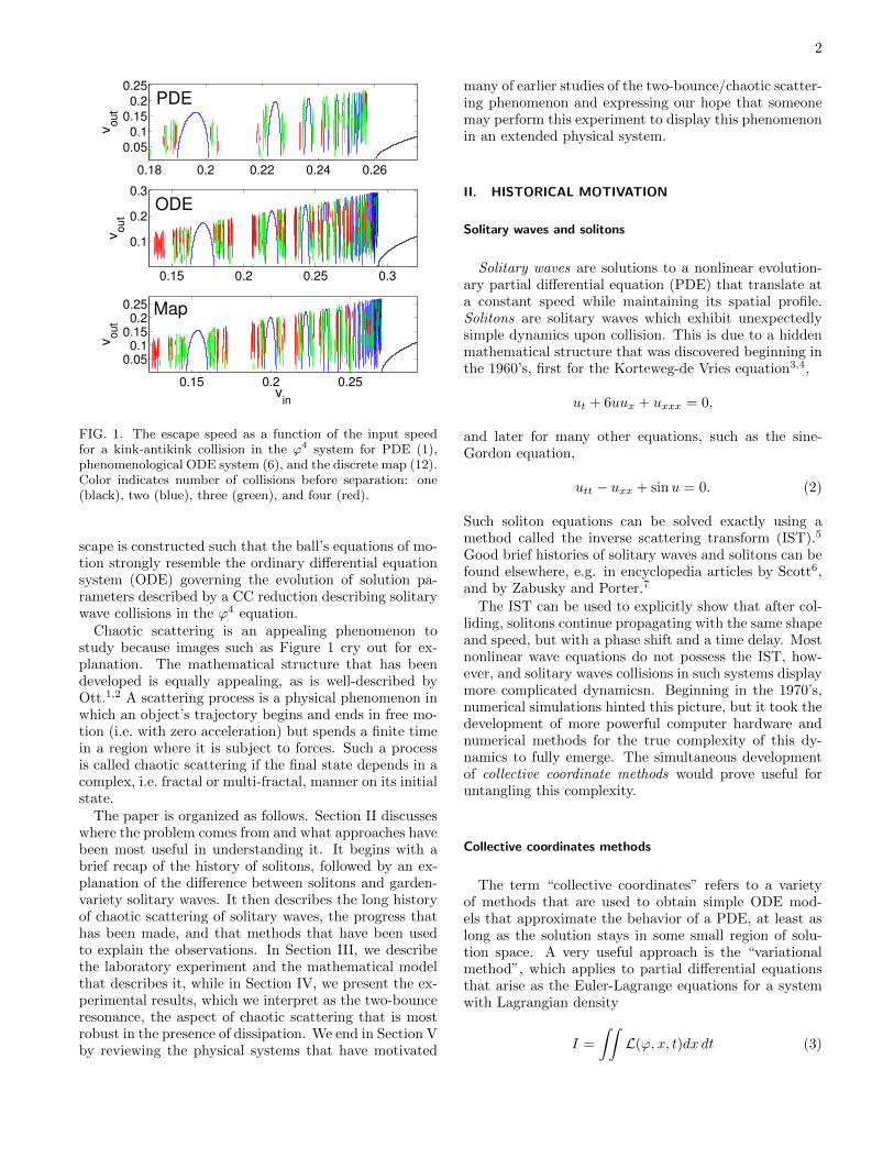
FIG. 1. The escape speed as a function of the input speedfor a kink-antikink collision in the ϕ4 system for PDE (1),phenomenological ODE system (6), and the discrete map (12).Color indicates number of collisions before separation: one(black), two (blue), three (green), and four (red).

scape is constructed such that the ball’s equations of mo-tion strongly resemble the ordinary differential equationsystem (ODE) governing the evolution of solution pa-rameters described by a CC reduction describing solitarywave collisions in the ϕ4 equation.

Chaotic scattering is an appealing phenomenon tostudy because images such as Figure 1 cry out for ex-planation. The mathematical structure that has beendeveloped is equally appealing, as is well-described byOtt.1,2 A scattering process is a physical phenomenon inwhich an object’s trajectory begins and ends in free mo-tion (i.e. with zero acceleration) but spends a finite timein a region where it is subject to forces. Such a processis called chaotic scattering if the final state depends in acomplex, i.e. fractal or multi-fractal, manner on its initialstate.

The paper is organized as follows. Section II discusseswhere the problem comes from and what approaches havebeen most useful in understanding it. It begins with abrief recap of the history of solitons, followed by an ex-planation of the difference between solitons and garden-variety solitary waves. It then describes the long historyof chaotic scattering of solitary waves, the progress thathas been made, and that methods that have been usedto explain the observations. In Section III, we describethe laboratory experiment and the mathematical modelthat describes it, while in Section IV, we present the ex-perimental results, which we interpret as the two-bounceresonance, the aspect of chaotic scattering that is mostrobust in the presence of dissipation. We end in Section Vby reviewing the physical systems that have motivated

many of earlier studies of the two-bounce/chaotic scatter-ing phenomenon and expressing our hope that someonemay perform this experiment to display this phenomenonin an extended physical system.

II. HISTORICAL MOTIVATION

Solitary waves and solitons

Solitary waves are solutions to a nonlinear evolution-ary partial differential equation (PDE) that translate ata constant speed while maintaining its spatial profile.Solitons are solitary waves which exhibit unexpectedlysimple dynamics upon collision. This is due to a hiddenmathematical structure that was discovered beginning inthe 1960’s, first for the Korteweg-de Vries equation3,4,

ut + 6uux + uxxx = 0,

and later for many other equations, such as the sine-Gordon equation,

utt − uxx + sinu = 0. (2)

Such soliton equations can be solved exactly using amethod called the inverse scattering transform (IST).5

Good brief histories of solitary waves and solitons can befound elsewhere, e.g. in encyclopedia articles by Scott6,and by Zabusky and Porter.7

The IST can be used to explicitly show that after col-liding, solitons continue propagating with the same shapeand speed, but with a phase shift and a time delay. Mostnonlinear wave equations do not possess the IST, how-ever, and solitary waves collisions in such systems displaymore complicated dynamicsn. Beginning in the 1970’s,numerical simulations hinted this picture, but it took thedevelopment of more powerful computer hardware andnumerical methods for the true complexity of this dy-namics to fully emerge. The simultaneous developmentof collective coordinate methods would prove useful foruntangling this complexity.

Collective coordinates methods

The term “collective coordinates” refers to a varietyof methods that are used to obtain simple ODE mod-els that approximate the behavior of a PDE, at least aslong as the solution stays in some small region of solu-tion space. A very useful approach is the “variationalmethod”, which applies to partial differential equationsthat arise as the Euler-Lagrange equations for a systemwith Lagrangian density

I =

∫∫L(ϕ, x, t)dx dt (3)

3

For example, solutions of the ϕ4 equation (1) minimizethe action due to

L =1

2ϕ2t −

1

2ϕ2x +

1

2ϕ2 − 1

4ϕ4

over all C1 function satisfying appropriate boundary con-ditions at infinity.

The variational method, due originally to Bondeson,8

works by constructing a solution ansatz whose spatialprofile depends on a small number of time-dependentparameters and minimizing the action (3) with respectto these parameters. The resulting equation is a finite-dimensional Lagrangian system of ODE governing theparameters’ evolution. Many examples and some gener-alizations are given in the review paper of Malomed.9

Numerical and analytical studies of solitary wave collisions

Solitary waves exist in the ϕ4 equation (1), which isnon-integrable, despite its clear similarity to the sine-Gordon equation (2). These “kink” waves are given by

ϕK(x, t; v) = tanhξ√2

, where ξ =x− vt√1− v2

for any − 1 < v < 1. (4)

The “antikink” solution is just ϕK(x, t, v) = −ϕK(x, t; v).Many papers have been written about kink-antikink

(KK) collisions in this system. In 1975, Kudryavtsev10

found numerically that when v = 0.1, the KK pair co-alesce into a single bound state at the origin which os-cillates irregularly and is slowly damped to zero. He ex-plained this with a formal argument based on potentialenergy which can be considered a first step toward anexplanatory collective coordinates model.

In 1979, Sugiyama11 performed additional experimentsfor a few values of v between 0.1 and 0.6. He found thatthose with speeds below a critical value vc ≈ 0.25 theKK pair merge into a localized bound state, while forv > vc, the pair collides inelastically. Careful examina-tion of his simulations showed that, upon collision, an os-cillatory mode (sometimes called a “shape mode”, sinceits effect is to alter the shape of the kink) is excited,which removes energy from the translation component.If the initial kinetic energy is less than the amount lostto the oscillatory mode, the KK pair can not escape toinfinity. If the v > vc, they will escape to infinity butwith reduced speed and with oscillations superimposed.He also derived the first CC model for this phenomenon,and used it in a formal calculation to determine vc inagreement with his numerical observations.

The shape mode is an eigenfunction for the lineariza-tion of equation (1) about the kink solution (4), and isgiven by

χ1(ξ) =

(3√2

) 12

sechξ√2

tanhξ√2

X

(a) U(X)

F(X)

X

dX

/dt

(b)

FIG. 2. (a) The potential and coupling function of equa-

tion (6). (b) The phase plane of the X − X subsystem, sepa-ratrix given by thick line.

and oscillates with frequency ω1 =√

32 . Sugiyama based

his CC ODE for this system on the ansatz

ϕ(x, t) =ϕK (x−X(t)) + ϕK (x+X(t))− 1

+A(t)χ1 (x−X(t))−A(t)χ1 (x+X(t)) .(5)

It leads to a two degree-of-freedom Hamiltonian systemfor the evolution of X(t) and A(t). The ODE system thatarises is somewhat complicated,11 but its fundamentalfeatures are captured by the simpler model system

X(t) + U ′(X) + cAF ′(X) = 0; (6a)

A(t) + ω2A+ cF (X) = 0, (6b)

where U(X) = e−2X − e−X and F (X) = e−X , plottedin Figure 2(a). This conserves an energy

E =1

2X2 + U(X) +

1

2

(A2 + ω2A2

)+ cAF (X).

The term U(X) is a potential energy describing the in-teraction of the two kinks, and was essentially derivedby Kudryavtsev.10 For large X, both F ′(X) and U ′(X)vanish, so that the kink and antikink centers ±X(t) moveat constant speed. The most important feature, for ourpurposes, is the phase diagram for X when c = 0, shownin Figure 2(b). The trajectories are level sets of the en-

ergy E = 12X

2 + U(X), with E < 0 on bounded orbits,a separatrix orbit with E = 0 and unbounded orbits forE > 0. We denote the separatrix orbit by XS(t), andnote it is an even function of time.

Figure 1 shows that this model qualitatively capturesmuch of the dynamics of solitary wave collisions in (1).Observe, however, a few fundamental differences. Whileboth systems conserve energy, in extended system (1),radiation (phonons) can carry energy away from the im-mediate vicinity of the kinks, effectively adding dissipa-tion. This can be seen in the figure, where only solutionsthat escape after four or fewer collisions are plotted. InODE (6), all solutions escape except for a set with mea-sure zero, while for the PDE, a significant fraction of so-lutions are trapped, due to energy loss to radiation. Theradiation also steals some energy from solutions that doescape, so that vout < vin even at the maxima of theresonance windows.

4

Also in 1979, Ablowitz, Kruskal, and Ladik reportedon a series of numerical experiments for a few differ-ent nonlinear Klein-Gordon equations of the form ϕtt −ϕxx + f(ϕ) = 0, including the ϕ4 equation and the sine-Gordon equation.12. Their numerical results were similarto Sugiyama’s but the paper ends with an observationwhich was to prove important: On certain velocity inter-vals below vc, the kink and antikink eventually separate,instead of forming a bound state as seen by Kudryavt-sev (from their References, it seems they had not seenSugiyama’s work at this point). When the initial veloc-ity is 0.3—greater than vc—the final velocity is 0.135.However, when the initial velocity is 0.2—less than vc,the final velocity is 0.155. They conclude “The reasonfor the apparent ‘resonance’ between these interactingaperiodic waves and the radiation is not yet fully under-stood.”

In 1983, Campbell et al.13 performed a more system-atic numerical sweep of initial velocities and found sig-nificantly more detailed structure. Their calculation re-vealed the black curve and the leftmost nine blue curvesin Figure 1. The black curve shows the final velocities ofall the solutions that escape after exactly one collision,i.e. those with initial speed above vc, which they esti-mate numerically to be 0.26. The blue curve shows thefinal velocities of those with exactly two collisions. Theycalled this phenomenon the two-bounce resonance.

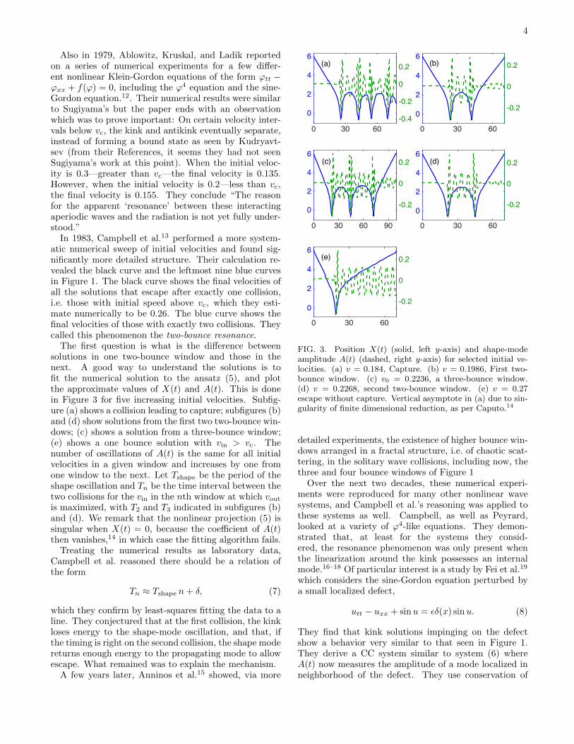
The first question is what is the difference betweensolutions in one two-bounce window and those in thenext. A good way to understand the solutions is tofit the numerical solution to the ansatz (5), and plotthe approximate values of X(t) and A(t). This is donein Figure 3 for five increasing initial velocities. Subfig-ure (a) shows a collision leading to capture; subfigures (b)and (d) show solutions from the first two two-bounce win-dows; (c) shows a solution from a three-bounce window;(e) shows a one bounce solution with vin > vc. Thenumber of oscillations of A(t) is the same for all initialvelocities in a given window and increases by one fromone window to the next. Let Tshape be the period of theshape oscillation and Tn be the time interval between thetwo collisions for the vin in the nth window at which vout

is maximized, with T2 and T3 indicated in subfigures (b)and (d). We remark that the nonlinear projection (5) issingular when X(t) = 0, because the coefficient of A(t)then vanishes,14 in which case the fitting algorithm fails.

Treating the numerical results as laboratory data,Campbell et al. reasoned there should be a relation ofthe form

Tn ≈ Tshape n+ δ, (7)

which they confirm by least-squares fitting the data to aline. They conjectured that at the first collision, the kinkloses energy to the shape-mode oscillation, and that, ifthe timing is right on the second collision, the shape modereturns enough energy to the propagating mode to allowescape. What remained was to explain the mechanism.

A few years later, Anninos et al.15 showed, via more

0 30 60

0

2

4

6(a)

0 30 60

0

2

4

6(b)

0 30 60 90

0

2

4

6(c)

0 30 60

0

2

4

6(d)

0 30 60

0

2

4

6(e)

-0.4

-0.2

0

0.2

-0.2

0

0.2

-0.2

0

0.2

-0.2

0

0.2

-0.2

0

0.2

FIG. 3. Position X(t) (solid, left y-axis) and shape-modeamplitude A(t) (dashed, right y-axis) for selected initial ve-locities. (a) v = 0.184, Capture. (b) v = 0.1986, First two-bounce window. (c) v0 = 0.2236, a three-bounce window.(d) v = 0.2268, second two-bounce window. (e) v = 0.27escape without capture. Vertical asymptote in (a) due to sin-gularity of finite dimensional reduction, as per Caputo.14

detailed experiments, the existence of higher bounce win-dows arranged in a fractal structure, i.e. of chaotic scat-tering, in the solitary wave collisions, including now, thethree and four bounce windows of Figure 1

Over the next two decades, these numerical experi-ments were reproduced for many other nonlinear wavesystems, and Campbell et al.’s reasoning was applied tothese systems as well. Campbell, as well as Peyrard,looked at a variety of ϕ4-like equations. They demon-strated that, at least for the systems they consid-ered, the resonance phenomenon was only present whenthe linearization around the kink possesses an internalmode.16–18 Of particular interest is a study by Fei et al.19

which considers the sine-Gordon equation perturbed bya small localized defect,

utt − uxx + sinu = εδ(x) sinu. (8)

They find that kink solutions impinging on the defectshow a behavior very similar to that seen in Figure 1.They derive a CC system similar to system (6) whereA(t) now measures the amplitude of a mode localized inneighborhood of the defect. They use conservation of

5

energy to derive an implicit formula for vc(ε) and ap-ply Campbell et al.’s reasoning to fit the time betweencollisions to the period of the secondary oscillator.

Reduction of collective coordinates to an iterated map

Beginning in 2004, Goodman and Haberman publisheda series of papers explaining the chaotic scattering indetail by reducing the CC ODE system to a discrete-time iterated map, called a separatrix map or scatteringmap.20,21 This was first done22 for the system studiedby Fei,19 because the the CC ODE system for equa-tion (8) has a small parameter ε that can be used ina perturbation analysis. Explicit formulas were foundto approximate the critical velocities and the two- andthree-bounce resonance, eliminating the need for datafitting as in equation (7). Over subsequent papers,23–25

the derivation of the map was streamlined and applied toother solitary waves systems and the model system (6).It was subsequently put in a more explicit form.26 Weoutline this last approach here.

Figure 4 depicts the results of one numerical simula-tion of the initial value problem (6) with the solitonsinitially far apart, propagating toward each other, andwith the shape mode unexcited, i.e X � 1, X < 0, andA = A = 0. Additionally X is small enough for cap-ture to occur. In this simulation, E(t) > 0 before thecollision, so that the solution is outside the separatrix inFigure 2(b), and crosses to the inside where E < 0 atthe first collision time t1. At each subsequent collisionE(t) jumps, reaching a plateau Ej between collisions attj−1 and tj , and escaping to infinity when E(t) > 0 onceagain. Upon each collision the amplitude and phase ofA(t) jump. We represent the solution before the collisionat time tj by the energy level Ej and by assuming

A(t) ∼ C (cj cosω(t− tj) + sj sinω(t− tj)) (9)

for t between tj−1 and tj , where setting the constant

C =c

ω

∫ ∞−∞

F (XS(t)) cosωtdt =c

ω

∫ ∞−∞

F (XS(t))eiωtdt

allows us to scale the variables to be O(1) in the finalform of the system. We seek a map (Ej+1, cj+1, sj+1) =M(Ej , cj , sj).

The map is constructed by building a matched asymp-totic expansion which alternates between “outer expan-sions” where X(t) is approximated by XS(t − tj), Fig-ure 2(b), and “inner expansions”. On the outer solution,valid when X(t) � 1, the modes exchange energy. Wefind, by variation of parameters, that outer solutions with“before-collision” condition (9) as t − tj → −∞, satisfythe “after-collision” condition

A(t) ∼ C (cj cosω(t− tj) + (sj − 1) sinω(t− tj))as t− tj → +∞, (10)

X(t)

E(t)

A(t)

E0E1E2

E3

E4

t1

t2

t3

t4

FIG. 4. Components used to construct the iterated map.Top X(t) showing the collision times tj . Middle: E(X, X)the energy of the X-component. Bottom: A(t).

and that

Ej+1 = Ej + C2ω2

(−1

2+ sj

)(11)

The change of energy is computed using a Melnikovintegral.20. Condition (10) is written in terms of (t− tj),whereas the form of the map requires (t − tj+1). Wecan compute the time between collisions by matchingbetween two the outer expansions connected by an in-

ner expansion, which gives tj+1− tj = αE−1/2j+1 + o(1) for

some α determined by matched asymptotics. This gives,approximately,[

cj+1

sj+1

]=

[cos θj+1 sin θj+1

− sin θj+1 cos θj+1

] [cj

sj − 1

],

where θj+1 = ω(tj+1 − tj).The discrete map possesses a conserved quantity H =

Ej + 12ω

2C2(c2j + s2j ) that allows us to eliminate Ej from

the system. Defining a complex variable zj = cj + isj ,the new map may be written

zj+1 = e−iα(H−|zj−1|2)−1/2

(zj − 1). (12)

Figure 1 shows that the map reproduces the qualita-tive and many quantitative features of the ODE systemand enables the determination of many of the featuresof the dynamics of system (6). For example, in the ex-periments depicted in Figure 1, the initial condition iszj = 0. Therefore, we may estimate the critical velocity:the solution is captured if E1 < 0, i.e. if v < vc = ωC,making use of equation (11). The analysis also allowsus to calculate approximate formulas for the centers ofthe two- and three bounce resonance windows, allowingthe computation of the constants in equation (7) withoutdata fitting.26

6

III. A PHYSICAL MODEL OF THE COLLECTIVECOORDINATE EQUATIONS

We wish to design a surface such that a ball confined toroll along that surface satisfies equations of motion simi-lar to system (6). We derive the evolution equations cor-responding for motion along a general surface and thendesign a surface that gives the desired dynamics.

A. The mathematical model

Consider the behavior of a point particle of mass mconfined to a surface z = h(x, y) and moving under theinfluence of constant gravity in the z-direction, and ignor-ing any friction or other dissipative mechanisms. We donot model in detail the rotation of the ball, instead not-ing that the rotational kinetic energy of a sphere rollingwith speed v is 2

5mv2. Adding this to the translational

component gives a total kinetic energy

T =7

5

m

2

(x2 + y2 + z2

)=

7

5

m

2

(x2 + y2 + (hxx+ hy y)

2).

The gravitational potential energy is just U = mgz =mgh(x, y). The evolution of a Lagrangian system withcoordinates qj is governed by the Euler-Lagrange equa-tions

d

dt

∂L

∂qj− ∂L

∂qj= 0 where L = T − U.

For this system, this gives, after some algebra,[xy

]+hxxx

2 + 2hxyxy + hyy y2 + g

1 + h2x + h2

y

[hxhy

]=

[00

]. (13)

where g = 57g. Under the assumption that the height

h(x, y) varies slowly (e.g. h(x, y) = h(δx, δy), δ � 1),this is approximately

x+ ghx(x, y) = 0;

y + ghy(x, y) = 0.(14)

Thus, when

g h(x, y) = U(x) +ω2

2y2 + εF (x)y, (15)

equation (14) is identical to equation (6). Such a sur-face is shown in Figure (5). Numerical simulations ofboth equations (13) and (14) show qualitatively the samechaotic scattering behavior (not shown here). Figure 5(a)shows a contour plot of the surface used.

We denote by x and y, respectively, the longitudinaland transverse, directions. To interpret the ODE, con-sider the case ε = 0, in which case the subspace y = y = 0is invariant. A ball that begins rolling down the centerof the surface with y = 0 stays along that line. Whenε > 0, this symmetry is broken, deflecting the longitudi-nal trajectory in the transverse direction. We will say a“bounce” occurs when the ball reaches a minimum in thelongitudinal direction.

FIG. 5. (a) Contour plot of the energy surface. (b) Photo-graph of the experimental surface.

B. Effects of dissipation

To account for experimental energy loss, we include a

viscous damping force ~Fdamp = −µ(x, y), which modifiesthe equations of motion to:

x+5µ

7mx+ ghx(x, y) = 0;

y +5µ

7my + ghy(x, y) = 0.

In Goodman, Holmes, and Weinstein27, a dissipative cor-rection to system (6) is derived to account for the ef-fect of radiative damping in nonlinear wave collisions. Itadds a term like F (X)

2A2A to the left-hand side of equa-

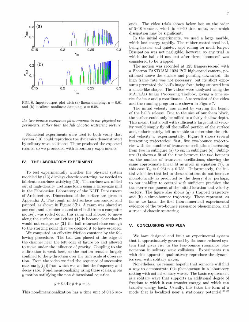
tion (6b). This damping term is strongly localized in X,only applying when the kink and antikink are close to-gether, and nonlinear in A so that small radiation dampsvery slowly. Both types of dissipation alter the fractalstructure displayed by the ODE system, as seen in fig-ure 6, but their effect is rather different. The localizeddamping preserves much more of the fine structure ofthe chaotic scattering, whereas the viscous damping de-stroys almost everything but the two-bounce resonancewindows. Their behavior for v near vc is also quite dif-ferent, with viscous damping reducing the final speed ofsolutions in the two-bounce solutions much more thanthe localized damping. We therefore expect to see mostly

7

0.15 0.2 0.25 0.30

0.1

0.2 (b)

vin

vout

0.15 0.2 0.25 0.30

0.1

0.2 (a)

vin

vout

FIG. 6. Input/output plot with (a) linear damping, µ = 0.01and (b) localized nonlinear damping, µ = 0.08.

the two-bounce resonance phenomenon in our physical ex-periments, rather than the full chaotic scattering picture.

Numerical experiments were used to both verify thatsystem (13) could reproduce the dynamics demonstratedby solitary wave collisions. These produced the expectedresults, so we proceeded with laboratory experiments.

IV. THE LABORATORY EXPERIMENT

To test experimentally whether the physical systemmodeled by (13) displays chaotic scattering, we needed tofabricate a surface satisfying (15). The surface was milledout of high-density urethane foam using a three-axis millin the Fabrication Laboratory of the NJIT Departmentof Architecture. Dimensions of the surface are given inAppendix A. The rough milled surface was sanded andpainted, as shown in Figure 5(b). A ramp was placed atone end, and a rubber coated steel ball (from a computermouse), was rolled down this ramp and allowed to movealong the surface until either (1) it became clear that itwould not escape, or (2) the ball returned close enoughto the starting point that we deemed it to have escaped.

We computed an effective friction constant by the fol-lowing procedure. The ball was placed at the edge ofthe channel near the left edge of figure 5b and allowedto move under the influence of gravity. Coupling to thex-direction is weak here, so the motion remains largelyconfined to the y-direction over the time scale of observa-tion. From the video we find the sequence of successivemaxima |y(tk)| from which we can find the frequency anddecay rate. Nondimensionalizing using these scales, givesy motion satisfying the non dimensional equation

y + 0.019 y + y = 0.

This nondimensionalization has a time unit of 0.15 sec-

onds. The video trials shown below last on the orderof 5–10 seconds, which is 30–60 time units, over whichdissipation may be significant.

In the initial experiments, we used a large marble,which lost energy rapidly. The rubber-coated steel ball,being heavier and quieter, kept rolling for much longer.Dissipation was not negligible, however, so any trial inwhich the ball did not exit after three “bounces” wasconsidered to be trapped.

The motion was recorded at 125 frames/second witha Photron FASTCAM 1024 PCI high-speed camera, po-sitioned above the surface and pointing downward. Itshigh frame rate was not necessary, but its short expo-sures prevented the ball’s image from being smeared intoa snake-like shape. The videos were analyzed using theMATLAB Image Processing Toolbox, giving a time se-ries for its x and y coordinates. A screenshot of the videoand the running program are shown in Figure 7.

The initial velocity was varied by varying the heightof the ball’s release. Due to the size of our foam block,the surface could only be milled to a fairly shallow depth.This meant that a ball with sufficiently large initial veloc-ity would simply fly off the milled portion of the surfaceand, unfortunately, left us unable to determine the crit-ical velocity vc experimentally. Figure 8 shows severalinteresting trajectories: first, five two-bounce trajecto-ries with the number of transverse oscillations increasingfrom two in subfigure (a) to six in subfigure (e). Subfig-ure (f) shows a fit of the time between the two bouncesvs. the number of transverse oscillations, showing thesame approximate linear fit as given in equation (7), inthis case Tn ≈ 0.961n + 0.755. Unfortunately, the ini-tial velocities that led to these solutions do not increasemonotonically as predicted by the theory, due, perhaps,to our inability to control with sufficient precision thetransverse component of the initial location and velocityvectors. The figure also shows (g) a trapped trajectoryand (h) a three-bounce trajectory. These represent, asfar as we knox, the first (non-numerical) experimentalevidence of the two-bounce resonance phenomenon, anda trace of chaotic scattering.

V. CONCLUSIONS AND PLEA

We have designed and built an experimental systemthat is approximately governed by the same reduced sys-tem that gives rise to the two-bounce resonance phe-nomenon in solitary wave collisions. Experiments runwith this apparatus qualitatively reproduce the dynam-ics seen with solitary waves.

Nonetheless, we remain hopeful that someone will finda way to demonstrate this phenomenon in a laboratorysetting with actual solitary waves. The basic requirementis a solitary wave that supports an additional degree offreedom to which it can transfer energy, and which cantransfer energy back. Usually, this takes the form of amode that is localized near a stationary potential19,22

8

FIG. 7. (Left) One frame from a movie of the experiment. (Center) The estimated trajectory up to time t ≈ 2. (Right) Theestimated coordinates as a function of time. See animation here.

0 1 2 3 40

20

40

60(a)

-15

0

15

0 2 40

20

40

60(b)

-15

0

15

0 2 4 60

20

40

60(c)

-15

0

15

0 2 4 60

20

40

60(d)

-15

0

15

0 2 4 6 80

20

40

60(e)

-15

0

15

0 5 100

20

40

60(g)

-15

0

15

0 2 4 6 80

20

40

60

n

T

(h)

-15

0

15

2 3 4 5 6

3

4

5

6

7(f)

FIG. 8. In all but (e) Longitudinal position x(t) (solid, left y-axis) and transverse coordinate y(t) (dashed, right y-axis) forselected initial velocities.(a-e) Two bounce trajectories. Eachcontains one transverse oscillation more than the one thatprecedes it. (f) Time between maxima of x(t) versus numberof transverse oscillations, with best-fit line. (g) “Captured”trajectory. (h) Three bounce trajectory.

or an internal mode of oscillation that moves with thewave,13,17 although this is not always necessary.28–30

Combing through some of the literature on this phe-nomenon, we find that many papers discuss the phys-ical systems described by their equations and mentionthat—perhaps—this phenomenon may be found in thesesystems. Experimental verification for some of these sys-tems is clearly impossible: Anninos et al.15 describe theϕ4 equation as describing the interactions of large-scaledomain walls in the universe. They admit, “Because thepossibility of head-on collisions is small in the real Uni-verse, our findings are not expected to have a profoundeffect cosmologically.” At the other extreme of scales,Kudryavtsev describes the ϕ4 system as a model for theHiggs field.10,31 Other unpromising applications for thetheory are information transport in brain microtubules,32

and various other quantum field theories.32,33

Other applications are perhaps closer to being exper-imentally realizable. In their original paper on the sub-ject, Campbell et al. suggest excitations in polymericchains and phase transitions in uniaxial ferroelectrics.13

Tan and Yang study the phenomenon in vector solitonsin optical fiber.23,28,29 Fei et al.’s numerical experimentspotentially describe the scattering of solitons off a de-fect in a long Josephson junction.19,22 Finally, Forinashet al. mention the denaturation of DNA.34 This list is farfrom exhaustive, and we encourage readers to think if anexperiment is possible in their favorite system.

ACKNOWLEDGEMENTS

The experiment was the focus of the Spring 2010 NJIT“capstone” course in applied mathematics, a class inwhich students perform laboratory experiments, learn

9

the math needed to model them and apply analyticaland numerical methods to that model to explain the re-sults. The first author was the instructor, and the oth-ers undergraduates enrolled in the course, who continuedworking on the project the following summer. The NSFCapstone Laboratory in the NJIT Department of Math-ematical Sciences was supported by NSF DMS-0511514.Thanks to Richard Haberman, Shane Ross, and LawrieVirgin for useful discussions and to Richard Garber andGene Dassing in the FabLab at the New Jersey School ofArchitecture, NJIT, for fabricating the surface and do-nating the material. Special thanks to David Campbellfor early discussions about the form of this article.

Appendix A: Specification of the experimental apparatus

To design the experimental surface, we performed nu-merical experiments of system (14), varying not just theparameters in the potential (6), but also the formulasfor the potentials U(x) and F (x), trying to ensure wecould observe interesting dynamics using the materialsavailable to us. The surface chosen was

h(x, y) = η(eax − ebx) + cy2 + εyedx

where the units of distance in all coordinate directions iscentimeters. The parameters chosen were

a = 0.389 cm−1, b = 0.306 cm−1, c = 0.0764 cm−1,

d = 0.306 cm−1, η = 3.27 cm, ε = 0.25.

1E. Ott and T. Tel, “Chaotic scattering: An introduction,” Chaos3, 417 (1993).

2E. Ott, Chaos in Dynamical Systems (Cambridge UniversityPress, 2002).

3N. Zabusky and M. Kruskal, “Interaction of ‘Solitons’ in a Colli-sionless Plasma and the Recurrence of Initial States,” Phys. Rev.Lett. 15, 240–243 (1965).

4C. Gardner, J. Greene, M. Kruskal, and R. Miura, “Methodfor solving the Korteweg-deVries equation,” Phys. Rev. Lett. 19,1095–1097 (1967).

5M. J. Ablowitz, D. J. Kaup, A. C. Newell, and H. Segur,“Method for solving the sine-Gordon equation,” Phys. Rev. Lett.30, 1262–1264 (1973).

6A. Scott, “Solitons, a brief history,” in The Encyclopedia of Non-linear Science, edited by A. Scott (Routledge, New York, 2004)pp. 852–855.

7N. J. Zabusky and M. A. Porter, “Soliton,” Scholarpedia 5, 2068(2010).

8A. Bondeson, M. Lisak, and D. Anderson, “Soliton Perturba-tions: A Variational Principle for the Soliton Parameters,” Phys-ica Scripta 20, 479–485 (1979).

9B. A. Malomed, “Variational methods in nonlinear fiber opticsand related fields,” Prog. Opt. 43, 71–193 (2002).

10A. E. Kudryavtsev, “Solitonlike solutions for a Higgs scalar field,”JETP Lett. 22, 82–83 (1975).

11T. Sugiyama, “Kink-Antikink Collisions in the Two-Dimensionalϕ4 Model,” Prog. Theor. Phys. 61, 1550–1563 (1979).

12M. J. Ablowitz, M. Kruskal, and J. Ladik, “Solitary Wave Col-lisions,” SIAM J. Appl. Math. 36, 428–437 (1979).

13D. K. Campbell, J. S. Schonfeld, and C. A. Wingate, “Resonancestructure in kink-antikink interactions in ϕ4 theory,” Phys. D 9,1–32 (1983).

14J. G. Caputo and N. Flytzanis, “Kink-antikink collisions in sine-Gordon and ϕ4 models: Problems in the variational approach,”Phys. Rev. A 44, 6219 (1991).

15P. Anninos, S. Oliveira, and R. Matzner, “Fractal structure inthe scalar λ(ϕ2−1)2 theory,” Phys. Rev. D 44, 1147–1160 (1991).

16M. Peyrard and M. Remoissenet, “Solitonlike excitations in aone-dimensional atomic chain with a nonlinear deformable sub-strate potential,” Phys. Rev. B 26, 2886–2899 (1982).

17M. Peyrard and D. K. Campbell, “Kink-antikink interactions ina modified sine-Gordon model,” Physica D 9, 33–51 (1983).

18M. Remoissenet and M. Peyrard, “Soliton dynamics in new mod-els with parameterized periodic double-well and asymmetric sub-strate potentials,” Phys. Rev. B 29, 3153–3166 (1984).

19Z. Fei, Y. Kivshar, and L. Vazquez, “Resonant kink-impurityinteractions in the sine-Gordon model,” Phys. Rev. A 45, 6019–6030 (1992).

20G. Zaslavsky, The Physics of Chaos in Hamiltonian Systems(Imperial College Press, 2007).

21M. Gidea, R. de la Llave, and T. Seara, “A General Mechanism ofDiffusion in Hamiltonian Systems: Qualitative Results,” (2014),arXiv:math-ds14050866.

22R. H. Goodman and R. Haberman, “Interaction of sine-Gordonkinks with defects: the two-bounce resonance,” Phys. D 195,303–323 (2004).

23R. H. Goodman and R. Haberman, “Vector-soliton collision dy-namics in nonlinear optical fibers,” Phys. Rev. E 71, 56605(2005).

24R. H. Goodman and R. Haberman, “Kink-antikink collisions inthe ϕ4 equation: The n-bounce resonance and the separatrixmap,” SIAM J. Appl. Dyn. Sys. 4, 1195–1228 (2005).

25R. H. Goodman and R. Haberman, “Chaotic scattering and then-bounce resonance in solitary-wave interactions,” Phys. Rev.Lett. 98, 104103 (2007).

26R. H. Goodman, “Chaotic scattering in solitary wave interac-tions: A singular iterated-map description,” Chaos 18, 023113(2008).

27R. H. Goodman, P. J. Holmes, and M. I. Weinstein, “Interactionof sine-Gordon kinks with defects: phase space transport in atwo-mode model,” Phys. D 161, 21–44 (2002).

28Y. Tan and J. Yang, “Complexity and regularity of vector-solitoncollisions,” Phys. Rev. E 64, 56616 (2001).

29J. Yang and Y. Tan, “Fractal structure in the collision of vectorsolitons,” Phys. Rev. Lett. 85, 3624–3627 (2000).

30P. Dorey, K. Mersh, T. Romanczukiewicz, and Y. Shnir, “Kink-Antikink Collisions in the ϕ6 Model,” Phys. Rev. Lett. 107(2011).

31T. I. Belova and A. E. Kudryavtsev, “Quasiperiodical OrbitsIn The Scalar Classical λϕ4 Field Theory,” Phys. D 32, 18–26(1988).

32B. Piette and W. Zakrzewski, “Scattering of sine-Gordon kinkson potential wells,” J. Phys. A 40, 5995–6010 (2007).

33K. Javidan, “Interaction of topological solitons with defects,” J.Phys. A 39, 10565–10574 (2006).

34K. Forinash, M. Peyrard, and B. A. Malomed, “Interaction ofdiscrete breathers with impurity modes,” Phys. Rev. E 49, 3400–3411 (1994).