General rights Copyright and moral rights for the publications made accessible in the public portal are retained by the authors and/or other copyright owners and it is a condition of accessing publications that users recognise and abide by the legal requirements associated with these rights.

• Users may download and print one copy of any publication from the public portal for the purpose of private study or research. • You may not further distribute the material or use it for any profit-making activity or commercial gain • You may freely distribute the URL identifying the publication in the public portal

If you believe that this document breaches copyright please contact us providing details, and we will remove access to the work immediately and investigate your claim.

Downloaded from orbit.dtu.dk on: May 17, 2018

A Matheuristic Approach to Integrate Humping and Pullout Sequencing Operations atRailroad Hump Yards

Haahr, Jørgen Thorlund; Lusby, Richard Martin

Published in:Networks

Link to article, DOI:10.1002/net.21665

Publication date:2016

Document VersionPeer reviewed version

Link back to DTU Orbit

Citation (APA):Haahr, J. T., & Lusby, R. M. (2016). A Matheuristic Approach to Integrate Humping and Pullout SequencingOperations at Railroad Hump Yards. Networks, 67(2), 126–138. DOI: 10.1002/net.21665

A Matheuristic Approach to Integrate Humping and Pullout

Sequencing Operations at Railroad Hump Yards

Department of Engineering Management

Technical University of Denmark

Jørgen Thorlund Haahr and Richard Martin Lusby

October 23, 2015

Abstract

This paper presents a novel matheuristic for solving the Hump Yard Block-to-Track Assignment

Problem. This is an important problem arising in the railway freight industry and involves scheduling

the transitions of a set of rail cars from a set of inbound trains to a set of outbound trains over

a certain planning horizon. It was also the topic of the 2014 challenge organised by the Railway

Applications Section of the Institute for Operations Research and the Management Sciences for which

the proposed matheuristic was awarded first prize. Our approach decomposes the problem into three

highly dependent subproblems. Optimization-based strategies are adopted for two of these, while the

third is solved using a greedy heuristic. We demonstrate the efficiency of the complete framework on

the official datasets, where solutions within 4-14% of a known lower bound (to a relaxed problem)

are found. We further show that improvements of around 8% can be achieved if outbound trains are

allowed to be delayed by up to two hours in the hope of ensuring an earlier connection for some of

the rail cars.

Keywords— Freight Train Optimization, Hump Yard Optimization, Block To Track Assignment,

Matheuristic, Mixed Integer Programming, Rolling Horizon

1 Introduction

This paper addresses the 2014 challenge posed by the Railway Applications Section (RAS) of the Institute

for Operations Research and the Management Sciences. The challenge focuses on an important problem

arising in the railway freight transportation industry known as the Hump Yard Block-to-Track Assignment

(HYBA). In particular, the problem requires one to consider, and schedule, the movements of a number

of rail cars through a classification or hump yard. The primary purpose of such a yard is to act as a

consolidation point, where rail cars arriving over a certain time horizon on a number of inbound trains

are rearranged, or classified, into groups of rail cars sharing the same destination. These groups are then

subsequently pulled out and combined to form new outbound trains, which remove rail cars from the

classification yard. A classification yard typically consists of four main components: an arrival yard, a

hump, a classification bowl, and a departure yard. During the processing of an inbound train each of its

1

rail cars is pushed over the hump, and, under the influence of gravity, and with the use of switches, rolls

to a pre-assigned classification track in the bowl. Bowls typically consist of multiple, parallel tracks of

possibly different lengths, where partial outbound trains can be assembled before being pulled together

to form outbound trains in the departure yard.

How to handle the steady flow of rail cars is of paramount importance to the efficiency of any clas-

sification yard. However, coordinating the processing of arriving inbound trains with the allocation of

classification tracks and the assembly of outbound trains is not a trivial task. All processes within the

yard are subject to a variety of different restrictions and, if scheduled poorly, can result in a situation

where rail cars needlessly wait long periods of time before leaving on an outbound train. The aim of the

HYBA is to process all cars in such a way that their average dwell time in the yard is minimized.

In this paper we present a novel solution approach for the HYBA problem. We propose a matheuristic

based on a decomposition of the problem into three distinct, highly dependent subproblems. A matheuris-

tic embeds mathematical programming techniques within a larger heuristic framework. For two of the

subproblems exact optimization-based solution strategies are employed. These are coupled with a heuris-

tic approach to the third, and the performance of the full heuristic is analysed using the official data sets.

These data sets are of a practical size and are based on a typical North American classification yard; each

considers a planning horizon of 42 days during which 702 inbound trains arrive (carrying in total 52,246

rail cars) to be processed. There are between 42 and 58 classification tracks on which to sort the rail cars,

which comprise 46 different destinations. Furthermore, there are 18 daily outbound trains. An outbound

train is scheduled to depart at the same time every day, and each destination is served by exactly one

outbound train. On such data sets, the proposed approach obtains acceptable solutions, within 4-14% of a

known lower bound (for a relaxed problem), for all data sets. We report run-times of at most 11 minutes.

To identify any bottlenecks at the considered classification yard we also perform a series of what-if

analyses. For example, we discuss the effects of having longer classification tracks or more capacity on

the outbound trains and compare the performance improvement to the base case. Finally, we show that

substantial reductions of around 8% in average dwell time can be made if it is possible to allow outbound

trains to be delayed by up to two hours. Given the relatively short run times of the approach, it is clearly

evident that the proposed methodology is equally applicable at the strategic level planning decisions

concerning railway classification yard design.

In what follows we describe aspects of the solution approach in more detail. We begin in Section 2 with

a short summary of previous research in this area. Section 3 provides a formal description of the problem,

while Section 4 introduces the models developed, together with their respective solution approaches. The

performance of the approach is the subject of Section 5, where we present results on the benchmark

instances provided. Finally, conclusions are drawn in Section 6.

2 Literature Review

The highly complex nature of hump yard planning makes it a perfect application for operations research

methodologies. Not surprisingly, various studies have been conducted on problems similar in nature, but

not identical, to the one considered in this paper. In this section we provide a brief review of the research

that is available in the literature and, where relevant, point out any differences from the problem at hand.

2

Furthermore, we restrict the review to those studies that concern hump yard planning on a microscopic

level only (i.e., planning the shunting movements within a single hump yard) since this is precisely the

problem we address in this paper. For a general introduction to shunting within hump yards the reader

is referred to [6, 10], while models that address hump yard planning at a macroscopic level (i.e., between

different yards), commonly known as the railroad blocking problem, can be found in [1, 2, 18].

Methods for hump yard planning are typically categorized as being either single or multi stage methods,

with the latter being by far the more researched. In a single stage method, each rail car arriving on an

inbound train can be humped to a classification track exactly once before it is pulled out to an outbound

train. Multi stage methods, on the other hand, allow rehumping (i.e., cars can be humped multiple times).

This additional flexibility is provided in the hope of obtaining a better sorting of the cars and, ultimately,

a more efficient use of the yard. Typically a so-called mixing track is specified, where any car assigned to

the mixing track can be pulled back to the hump and classified again.

The works [3, 4, 5] specifically address the problems of sorting and classifying rail cars at a hump yard

using the mixed track concept. All papers restrict their attention to scheduling the classification bowl of

the hump yard only. A noticeable difference between this problem and the one that we consider is that

the formation of the outbound trains happens directly on the tracks of the classification bowl. Typically

a track of the bowl is dedicated to a specific outbound train and the cars destined for the outbound train

appear on the train in the order they are humped to the track. As reserving a classification track for a

single outbound train claims significant sorting capacity, it is impractical to allocate an outbound train

an entire track from the arrival of its first car until its departure. As such, a number of mixing tracks is

used to temporarily hold cars for different trains. The cars on such tracks are then rehumped.

In [3], the authors describe an integer programming formulation that attempts to minimize the number

of rehumpings that must be performed. These extra shunting movements are termed roll-ins by the

authors. The model is solved using a branch-and-price algorithm and tested on 192 real-life instances

from the Hallsberg marshalling (hump) yard in Sweden. The authors provide a direct comparison with

a compact integer programming formulation and demonstrate the superiority of the column generation

procedure. Reference [4] extends this methodology to model situations in which the arriving rail cars each

belong to a certain block, and these blocks must appear in a pre-specified order on the outbound train.

Again, the Hallsberg hump yard in Sweden forms the basis of the computational study, where 50 instances

with a planning horizon of three days are considered. An extension to [3] is also considered in [5], where

a new arc-based model is presented, along with a rolling-horizon solution framework and an analysis of

yard capacity.

The problem we consider shares strong similarities with that considered in [3, 4, 5]; however, there

are several key differences. First, the incoming sequence of cars is not fixed in our problem (i.e., we can

decide the order in which to process the inbound trains), we are not allowed to rehump cars, and we must

coordinate the assembly of outbound trains using a set of pullback engines. That is, the assignment of a

rail car to a classification track does not implicitly indicate the outbound train, nor the order in which it

appears on an outbound train.

Identifying an efficient sorting of inbound rail cars at classification yards is also the focus of [8]. The

authors adopt a more theoretical approach to the problem and prove that the problem of finding the

minimum number of tracks required to sort a set of arriving rail cars into blocks of cars that can be

3

pulled out in a specific order from the classification tracks is NP-complete. This topic is also addressed

by [7, 12, 17]. In [12], the authors develop a novel encoding strategy for classification schedules, discuss

its complexity, and present algorithms that can be used to solve practical rail car classification problems.

Theoretical aspects of rail car classification are also considered in [17]. In addition, the author describes

several practical extensions of the problem, and an integer programming formulation is developed to solve

the classification problem. Finally, [7] completes an open proof from [12] and show that identifying optimal

classification schedules in constructing one long outbound train from multiple inbound trains is NP-Hard.

Dirnberger and Barkan [9] consider improving the performance of classification yards and introduce

the concept of so-called lean railroading. This approach adapts production management strategies to

the railroad environment. The pull-down, or outbound train assembly, process is identified as the main

bottleneck, and the authors suggest that to improve the performance of classification yards emphasis

should be placed on identifying quality sorting strategies instead of merely measuring the number of cars

processed at the hump. Studies reported in the paper suggest that capacity for train assembly can be

increased by as much as 26%.

Attempts to improve the connection reliability of hump yards are provided in the two part series

of papers [13, 14]. Determining which cars to process at the hump, and in which order, is critical in

ensuring that cars meet specific (i.e., the earliest) outbound departures. The first paper [13] considers

the relationship between priority-based-classification and dynamic car scheduling to produce a reliable

service. The author emphasizes the need for better information to be available at the time at which a car

is humped (ideally the outbound train to which it will be assigned). This can be coupled with a more

efficient block-to-track assignment to ensure that the classification yard is being used to its full potential.

This is precisely the topic of the second paper [14]. The author describes a dynamic car block-to-track

assignment strategy based on delivery commitment rather than a first-in-first-out strategy. In other words,

cars with very little schedule slack should have access to the first available outbound train capacity. The

proposed heuristic framework sorts cars by outbound train and destination yard block as opposed to just

destination yard block, giving greater knowledge regarding the exact make-up of each outbound train.

He et al. [11] present a Mixed Integer Program (MIP) model for optimizing single stage hump yard

operations (i.e., no rehumping), from inbound train classification to outbound train assembly and depar-

ture. The model also appears to account for outbound block standing orders and limits on the number

of pullback engines available to do the sorting. Due to its size and complexity, the authors present a

decomposition-based heuristic and discuss its performance on several practical instances arising in China.

The problems considered up to 170 inbound trains per day (with up to 8,000 cars per day in total). The

objective essentially minimizes a combination of the dwell time of the rail cars in the yard and delays to

outbound trains. Running times of the algorithm are reported to be within 10 minutes.

Finally, simulation models for hump yard planning are described in [15, 16]. The focus in these pa-

pers is not on optimizing the hump yard schedules, but rather in identifying bottlenecks in the existing

infrastructure (i.e., the number of cars that can be handled) with existing scheduling strategies.

4

8:00 8:00 8:00 8:00 8:00

12:00 12:00 12:00

16:00 16:00 16:00 16:00 16:00

New York Boston

Arrival Yard Classification Yard Departure Yard

Hum

p

9:00 Departure

8:05

8:04

8:03

12:00 12:00 12:00

16:00 16:00 16:00 16:00 16:00

Hum

p

8:02 8:01

8:05

8:24

8:03

12:00 12:00 12:00

16:00 16:00 16:00 16:00 16:00H

um

p

8:24 8:24

Figure 1: An example of a problem instance illustrating the railcars, the three different yards in threetimesteps on the vertical axis. Railcars are represented as dashed, dotted and solid boxes correspondingto their assigned destinations (or block IDs). Assume one car can be processed by the hump every minute,and that the pullout time is 20 minutes. Three different inbound trains with distinct arrival times (8:00,12:00 and 16:00) and one outbound train departing at 9:00 are shown. The top portion shows the initialstate, where nothing is assigned. The middle portion shows an inbound train has been processed andbowl tracks have been assigned to the railcars. The bottom portion shows a cut has been pulled out andassigned to meet the departing train.

3 Problem Description

The considered problem has been introduced and defined by the Railway Application Section Competition

2014 [19]. In this section we present a standalone definition of the problem as well as introduce the notation

we use throughout the paper. We reuse the notation and concepts of the original formulation to a great

extent. An illustration of the problem mechanics is shown in Figure 1.

We assume that there is a set of inbound trains I arriving at the hump yard over a given time horizon.

Each inbound train consists of a coupled, ordered sequence of railcars that will be separated at the hump

in the yard. Each train i ∈ I arrives at the hump yard at a given time ai, given in seconds from the start of

the horizon. Note that this does not indicate the time at which it will be humped; a train can wait in the

arrival yard as long as is necessary. The arrival yard is assumed to have infinite capacity. We denote the set

of railcars by Ci for a given inbound train i ∈ I. Naturally, the full set of cars to be processed is therefore

C :=⋃i Ci. Along with a length lc, each car c ∈ C has a known block ID (henceforth referred to as just

block), denoted bc. This indicates the car’s next destination: for example BOS for Boston and PHX for

Phoenix. The set of all blocks is given by B. As an example, Figure 2 indicates the composition of the first

10 inbound trains: in other words, the number of cars of different outbound blocks on each train. The bar

chart provides a summary of the block counts only. On any given inbound train, the cars associated with

a certain block are not usually in consecutive order, but distributed throughout the train. This random

pattern is representative for the inbound trains in our dataset, i.e., we rarely see long sequences of cars

with identical blocks.

5

0 20 40 60 80 100

1

2

3

4

5

6

7

8

9

10

Car Count

Inb

ou

nd

Tra

inN

um

ber

Inbound Train by Outbound Block

Figure 2: The different outbound blocks on each of the first 10 inbound trains. Different patterns corre-spond to different blocks.

Every inbound train i ∈ I must be processed, i.e., each of the cars c ∈ Ci must be decoupled, pushed

over a hump, and moved to an available track in the classification bowl. Note that the process can be

paused for a period, i.e., a partially decoupled inbound train can be stopped on the hump, e.g., if no track

with sufficient space is available in the classification bowl.

It is assumed that the bowl consists of a set of parallel tracks T , where each t ∈ T has a known length

γt, and operates as a first-in-first-out queue. The tracks of the bowl are be used to sort the cars into lines

of cars. A line is a sequence of cars of the same block and which are assigned to the same pullout (i.e.,

they appear on the same outbound train).

When humping a train several constraints must be respected. First, it is assumed two hump engines

are available to perform the humping operations; one pulls cars from an inbound train to the hump, while

the other is used to retrieve inbound trains from the arrival yard, i.e., bring them to the humping point.

An inbound train’s humping time refers to the time at which its first car is humped and two consecutive

humpings must therefore be separated by some minimum duration. This duration is equal to either the

minimum time required to hump all of the first train’s cars (each car is assumed to take a constant time,

λ seconds, to hump), or the time required to retrieve the next inbound train from the arrival yard, again

constant and equal to δ seconds, whichever is the longer. In addition, all of a train’s cars must be humped

before any other train can be humped, i.e, no train can be partially humped; it is considered to be an

atomic operation.

Railcars that are coupled together are pulled from bowl tracks and appended to an awaiting outbound

train. Each outbound train o ∈ O is scheduled to depart at the given time do and has a maximum length

ηo of railcars that it can carry. An outbound train has a predetermined route through specific destinations

(i.e., blocks) which is why the assigned railcars must conform to a standing order, that stipulates the order

6

in which the railcar destinations (blocks) must appear on the outbound train.

Outbound trains are built in the departure yard using three available pullout engines. Pullout engines

move so-called cuts of rail cars from the bowl to the departure yard. A cut simply refers to a sequence

of lines that adhere to the standing order of the designated outbound train. Like hump engines, several

restrictions exist for the pullout engines. First, pullouts from the same bowl track must be separated in

time by a minimum duration to allow a smooth operation. Second, pullouts to the same outbound train

must also be separated in time as multiple engines cannot build the same departure train simultaneously.

Third, consecutive pullouts by the same engine must also be spaced by a minimum duration, corresponding

to the time required to perform one job, which we denote ρ.

Finally, an outbound train can only be built within a certain time window of its scheduled departure

time; e.g., for the considered problem, an outbound train can start to be assembled, at the earliest, 4

hours prior to its departure. However, we also consider an extension to the problem where departures can

be delayed. Note that delaying a given outbound train will increase the dwell time for all cars assigned

to that departure; however, it will also potentially reduce the dwell time of other rail cars that would

otherwise miss the connection if it departed on time.

The objective of this problem is to determine the humping sequence of the inbound trains, which bowl

track to use when humping each car, and the schedule for the pullout engines (i.e., how each outbound

train should be built) such that all constraints are satisfied and the average dwell time of the cars in

the yard is minimized. In other words, we need to determine an itinerary for each individual railcar (i.e.,

hump time, assigned bowl track, pullout time and outbound train), such that none of the constraints are

violated.

4 Modelling & Methodology

Given the problem’s size and complexity, it is extremely difficult to construct a tractable mathematical

model for the entire problem. Hence, we decompose the problem into three smaller, interdependent sub-

problems. which we term the Hump Sequencing Problem (HSP), the Block to Track Assignment Problem

(BTAP), and The Pullout Allocation Problem (PAP), respectively. For the HSP and the PAP we describe

MIP based optimization approaches, while we present a simple greedy heuristic for the BTAP. In this

section we elaborate on each of these problems as well as the proposed methodology to solve them.

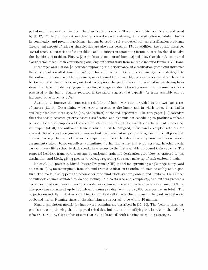
To set the context we provide a brief overview of the proposed methodology before going into specific

details regarding each of the subproblems. Figure 3 illustrates the flow of the proposed approach. We begin

by finding an arrival sequence for the inbound trains, e.g., using the HSP, and this remains fixed for the

remainder of the algorithm. That is, after finding this processing sequence we never revise the humping

order of the inbound trains. Cars are then iteratively humped into the bowl and assigned classification

tracks using the BTAP. As soon as a car cannot be humped into the classification bowl, possibly due to a

lack of space or no free tracks, the humping process is halted and pullouts are scheduled to make space in

the bowl. Which pullouts to perform are decided by the PAP. Note that during an iteration the PAP and

BTAP are not necessarily considering the bowl at the exact same time or time period. In general when

the BTAP pauses at time t, e.g., due to lack of space or compatible tracks, the PAP will consider pullouts

that occur before t.

7

StopStop

Perform PulloutsPerform Pullouts

Sequence Inbound TrainsSequence Inbound TrainsStartStart

Car To Hump?Car To Hump?

Assign Classification TrackAssign Classification Track

Track Assigned?Track Assigned?

Cars Remaining?Cars Remaining?

Get Next Car To HumpGet Next Car To Hump

No

No

No

Yes Yes

Yes

Figure 3: An overview of the proposed solution framework.

This process of humping cars and performing pullouts continues until there are no cars left to process.

To provide a quality measure on the solutions found, in Section 4.1, we show how one can obtain lower

bounds on the minimum average car dwell time. The lower bounds, albeit potentially weak, provide some

sort of quality measure for the obtained solutions. Sections 4.2-4.4 are dedicated to the HSP, BTAP, and

the PAP, respectively.

4.1 Lower Bounds

In order to verify the quality of the solutions produced by the matheuristic it is important to obtain a

lower bound on the total dwell time. Here we describe two rather simple approaches for generating such

bounds. Both bounds assume that outbound train departure times are fixed.

The first lower bound assumes that all outbound trains have infinite capacity, that all trains can be

humped immediately, and that there are neither capacity nor ordering restrictions in the classification

bowl. It does, however, respect the humping rate of the cars; the time at which any car is assumed to be

available for a departure is a certain duration after the arrival time of the train it is on. This duration is

the time needed to hump the cars ahead of it on the train.

The lower bound on average dwell time (in hours) is calculated as follows:

LB =(∑i∈I

∑c∈Ci dc − ai)

3600 · |C|, (1)

8

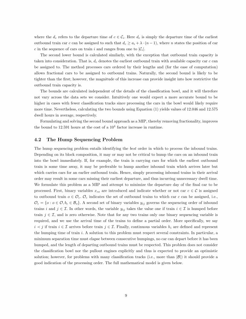
where the dc refers to the departure time of c ∈ Ci. Here dc is simply the departure time of the earliest

outbound train car c can be assigned to such that dc ≥ ai + λ · (n− 1), where n states the position of car

c in the sequence of cars on train i and ranges from one to |Ci|.The second lower bound is calculated similarly, with the exception that outbound train capacity is

taken into consideration. That is, dc denotes the earliest outbound train with available capacity car c can

be assigned to. The method processes cars ordered by their lengths and (for the ease of computation)

allows fractional cars to be assigned to outbound trains. Naturally, the second bound is likely to be

tighter than the first; however, the magnitude of this increase can provide insight into how restrictive the

outbound train capacity is.

The bounds are calculated independent of the details of the classification bowl, and it will therefore

not vary across the data sets we consider. Intuitively one would expect a more accurate bound to be

higher in cases with fewer classification tracks since processing the cars in the bowl would likely require

more time. Nevertheless, calculating the two bounds using Equation (1) yields values of 12.046 and 12.575

dwell hours in average, respectively.

Formulating and solving the second bound approach as a MIP, thereby removing fractionality, improves

the bound to 12.591 hours at the cost of a 104 factor increase in runtime.

4.2 The Hump Sequencing Problem

The hump sequencing problem entails identifying the best order in which to process the inbound trains.

Depending on its block composition, it may or may not be critical to hump the cars on an inbound train

into the bowl immediately. If, for example, the train is carrying cars for which the earliest outbound

train is some time away, it may be preferable to hump another inbound train which arrives later but

which carries cars for an earlier outbound train. Hence, simply processing inbound trains in their arrival

order may result in some cars missing their earliest departure, and thus incurring unnecessary dwell time.

We formulate this problem as a MIP and attempt to minimize the departure day of the final car to be

processed. First, binary variables xco are introduced and indicate whether or not car c ∈ C is assigned

to outbound train o ∈ Oc. Oc indicates the set of outbound trains to which car c can be assigned, i.e.,

Oc = o : o ∈ O, bc ∈ Bo. A second set of binary variables yij governs the sequencing order of inbound

trains i and j ∈ I. In other words, the variable yij takes the value one if train i ∈ I is humped before

train j ∈ I, and is zero otherwise. Note that for any two trains only one binary sequencing variable is

required, and we use the arrival time of the trains to define a partial order. More specifically, we say

i ≺ j if train i ∈ I arrives before train j ∈ I. Finally, continuous variables hi are defined and represent

the humping time of train i. A solution to this problem must respect several constraints. In particular, a

minimum separation time must elapse between consecutive humpings, no car can depart before it has been

humped, and the length of departing outbound trains must be respected. This problem does not consider

the classification bowl nor the pullout engines explicitly and thus is expected to provide an optimistic

solution; however, for problems with many classification tracks (i.e., more than |B|) it should provide a

good indication of the processing order. The full mathematical model is given below.

9

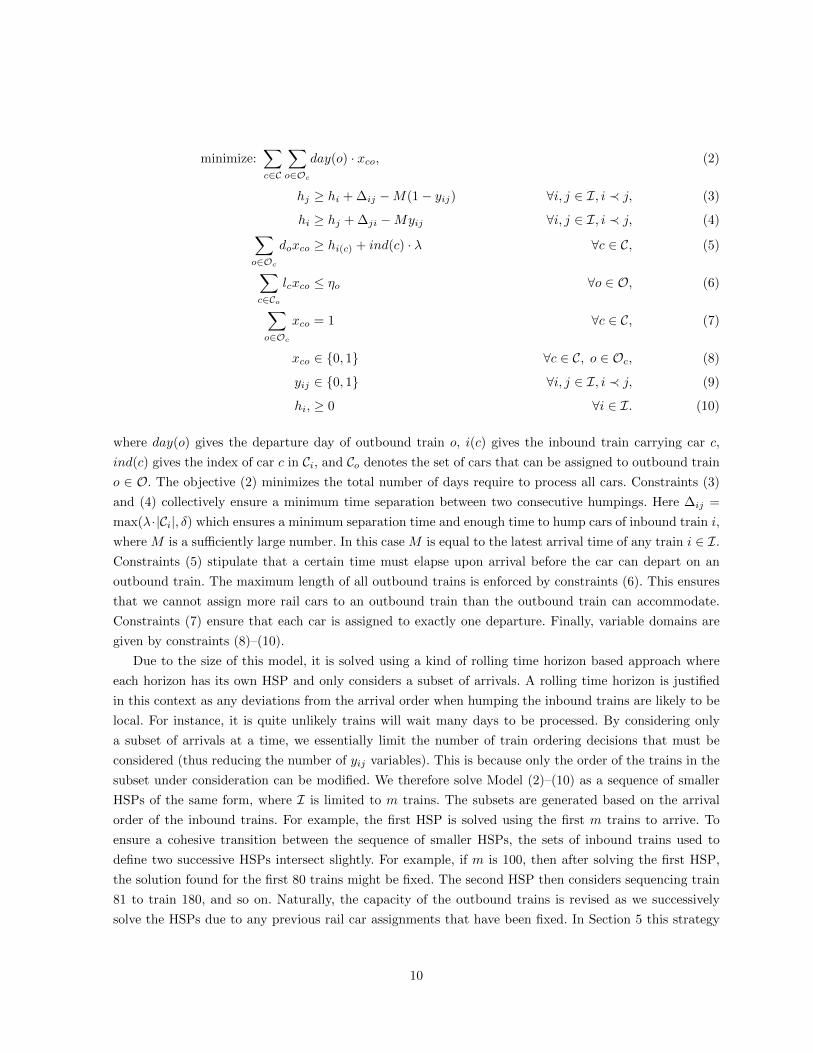
minimize:∑c∈C

∑o∈Oc

day(o) · xco, (2)

hj ≥ hi + ∆ij −M(1− yij) ∀i, j ∈ I, i ≺ j, (3)

hi ≥ hj + ∆ji −Myij ∀i, j ∈ I, i ≺ j, (4)∑o∈Oc

doxco ≥ hi(c) + ind(c) · λ ∀c ∈ C, (5)

∑c∈Co

lcxco ≤ ηo ∀o ∈ O, (6)

∑o∈Oc

xco = 1 ∀c ∈ C, (7)

xco ∈ 0, 1 ∀c ∈ C, o ∈ Oc, (8)

yij ∈ 0, 1 ∀i, j ∈ I, i ≺ j, (9)

hi, ≥ 0 ∀i ∈ I. (10)

where day(o) gives the departure day of outbound train o, i(c) gives the inbound train carrying car c,

ind(c) gives the index of car c in Ci, and Co denotes the set of cars that can be assigned to outbound train

o ∈ O. The objective (2) minimizes the total number of days require to process all cars. Constraints (3)

and (4) collectively ensure a minimum time separation between two consecutive humpings. Here ∆ij =

max(λ·|Ci|, δ) which ensures a minimum separation time and enough time to hump cars of inbound train i,

where M is a sufficiently large number. In this case M is equal to the latest arrival time of any train i ∈ I.

Constraints (5) stipulate that a certain time must elapse upon arrival before the car can depart on an

outbound train. The maximum length of all outbound trains is enforced by constraints (6). This ensures

that we cannot assign more rail cars to an outbound train than the outbound train can accommodate.

Constraints (7) ensure that each car is assigned to exactly one departure. Finally, variable domains are

given by constraints (8)–(10).

Due to the size of this model, it is solved using a kind of rolling time horizon based approach where

each horizon has its own HSP and only considers a subset of arrivals. A rolling time horizon is justified

in this context as any deviations from the arrival order when humping the inbound trains are likely to be

local. For instance, it is quite unlikely trains will wait many days to be processed. By considering only

a subset of arrivals at a time, we essentially limit the number of train ordering decisions that must be

considered (thus reducing the number of yij variables). This is because only the order of the trains in the

subset under consideration can be modified. We therefore solve Model (2)–(10) as a sequence of smaller

HSPs of the same form, where I is limited to m trains. The subsets are generated based on the arrival

order of the inbound trains. For example, the first HSP is solved using the first m trains to arrive. To

ensure a cohesive transition between the sequence of smaller HSPs, the sets of inbound trains used to

define two successive HSPs intersect slightly. For example, if m is 100, then after solving the first HSP,

the solution found for the first 80 trains might be fixed. The second HSP then considers sequencing train

81 to train 180, and so on. Naturally, the capacity of the outbound trains is revised as we successively

solve the HSPs due to any previous rail car assignments that have been fixed. In Section 5 this strategy

10

is compared against the greedy approach of simply processing trains in their arrival order.

Finally, it is important to note that the solution to this problem might not be implementable in

practice. Since the model does not consider classification tracks nor the pullout operations, there is no

guarantee rail cars can actually leave on the departure to which they have been assigned in the HSP. The

model is only used to provide an indication of hump sequencing order and is potentially quite optimistic.

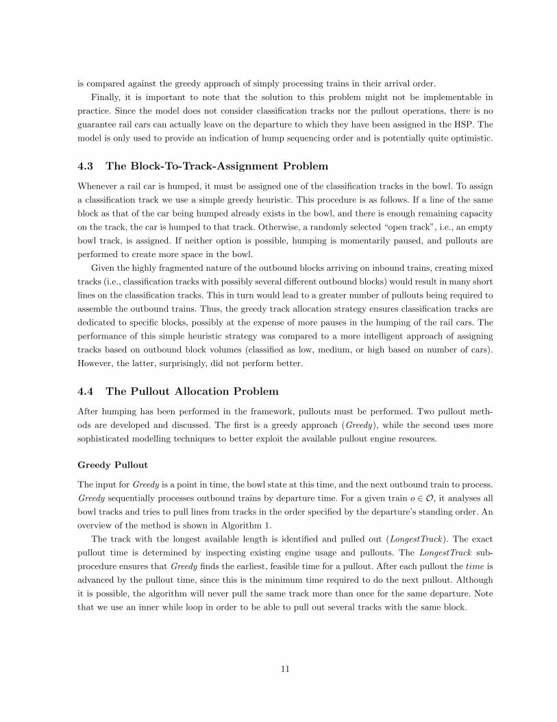
4.3 The Block-To-Track-Assignment Problem

Whenever a rail car is humped, it must be assigned one of the classification tracks in the bowl. To assign

a classification track we use a simple greedy heuristic. This procedure is as follows. If a line of the same

block as that of the car being humped already exists in the bowl, and there is enough remaining capacity

on the track, the car is humped to that track. Otherwise, a randomly selected “open track”, i.e., an empty

bowl track, is assigned. If neither option is possible, humping is momentarily paused, and pullouts are

performed to create more space in the bowl.

Given the highly fragmented nature of the outbound blocks arriving on inbound trains, creating mixed

tracks (i.e., classification tracks with possibly several different outbound blocks) would result in many short

lines on the classification tracks. This in turn would lead to a greater number of pullouts being required to

assemble the outbound trains. Thus, the greedy track allocation strategy ensures classification tracks are

dedicated to specific blocks, possibly at the expense of more pauses in the humping of the rail cars. The

performance of this simple heuristic strategy was compared to a more intelligent approach of assigning

tracks based on outbound block volumes (classified as low, medium, or high based on number of cars).

However, the latter, surprisingly, did not perform better.

4.4 The Pullout Allocation Problem

After humping has been performed in the framework, pullouts must be performed. Two pullout meth-

ods are developed and discussed. The first is a greedy approach (Greedy), while the second uses more

sophisticated modelling techniques to better exploit the available pullout engine resources.

Greedy Pullout

The input for Greedy is a point in time, the bowl state at this time, and the next outbound train to process.

Greedy sequentially processes outbound trains by departure time. For a given train o ∈ O, it analyses all

bowl tracks and tries to pull lines from tracks in the order specified by the departure’s standing order. An

overview of the method is shown in Algorithm 1.

The track with the longest available length is identified and pulled out (LongestTrack). The exact

pullout time is determined by inspecting existing engine usage and pullouts. The LongestTrack sub-

procedure ensures that Greedy finds the earliest, feasible time for a pullout. After each pullout the time is

advanced by the pullout time, since this is the minimum time required to do the next pullout. Although

it is possible, the algorithm will never pull the same track more than once for the same departure. Note

that we use an inner while loop in order to be able to pull out several tracks with the same block.

11

Algorithm 1

1: procedure GreedyPullout(departure, bowl, time)2: for b ∈ BlockStandingOrder(departure) do3: (track, len) ←LongestTrack(bowl, b, time)4: while len > 0 do5: next ← NextPulloutTime(track,

departure, time)6: bowl ← PerformPullout(bowl, track,

departure, next)7: time ← next8: (track, length) ←LongestTrack(bowl,

b, time)

14:00

Departures

14:30

14:00

Naive Approach

14:30

14:00

MIP Approach

14:30

13:00 13:00 14:00 13:00 13:00

14:00 14:00 14:00 14:00

Railcars on bowl tracks

Figure 4: A comparison of the Greedy and MIP pullout approaches. In the top left portion the currentbowl tracks are illustrated, and in the top right portion the scheduled departures are depicted. In thisexample one pullout engine is available and requires one hour per pullout job, and each departure can bebuilt two hours in advance. The Greedy method processes the departures iteratively by departure time,thus in this example nothing is assigned to the second departures as the engine has been fully assignedup until 14:00. The MIP method, however, identifies a solution that shares the engines such that the totalnumber of pulled railcars is maximized.

12

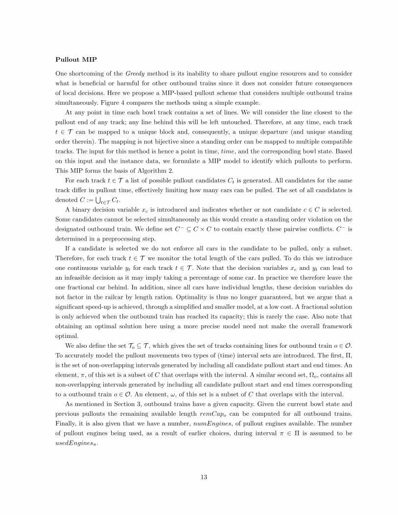
Pullout MIP

One shortcoming of the Greedy method is its inability to share pullout engine resources and to consider

what is beneficial or harmful for other outbound trains since it does not consider future consequences

of local decisions. Here we propose a MIP-based pullout scheme that considers multiple outbound trains

simultaneously. Figure 4 compares the methods using a simple example.

At any point in time each bowl track contains a set of lines. We will consider the line closest to the

pullout end of any track; any line behind this will be left untouched. Therefore, at any time, each track

t ∈ T can be mapped to a unique block and, consequently, a unique departure (and unique standing

order therein). The mapping is not bijective since a standing order can be mapped to multiple compatible

tracks. The input for this method is hence a point in time, time, and the corresponding bowl state. Based

on this input and the instance data, we formulate a MIP model to identify which pullouts to perform.

This MIP forms the basis of Algorithm 2.

For each track t ∈ T a list of possible pullout candidates Ct is generated. All candidates for the same

track differ in pullout time, effectively limiting how many cars can be pulled. The set of all candidates is

denoted C :=⋃t∈T Ct.

A binary decision variable xc is introduced and indicates whether or not candidate c ∈ C is selected.

Some candidates cannot be selected simultaneously as this would create a standing order violation on the

designated outbound train. We define set C− ⊆ C × C to contain exactly these pairwise conflicts. C− is

determined in a preprocessing step.

If a candidate is selected we do not enforce all cars in the candidate to be pulled, only a subset.

Therefore, for each track t ∈ T we monitor the total length of the cars pulled. To do this we introduce

one continuous variable yt for each track t ∈ T . Note that the decision variables xc and yt can lead to

an infeasible decision as it may imply taking a percentage of some car. In practice we therefore leave the

one fractional car behind. In addition, since all cars have individual lengths, these decision variables do

not factor in the railcar by length ration. Optimality is thus no longer guaranteed, but we argue that a

significant speed-up is achieved, through a simplified and smaller model, at a low cost. A fractional solution

is only achieved when the outbound train has reached its capacity; this is rarely the case. Also note that

obtaining an optimal solution here using a more precise model need not make the overall framework

optimal.

We also define the set To ⊆ T , which gives the set of tracks containing lines for outbound train o ∈ O.

To accurately model the pullout movements two types of (time) interval sets are introduced. The first, Π,

is the set of non-overlapping intervals generated by including all candidate pullout start and end times. An

element, π, of this set is a subset of C that overlaps with the interval. A similar second set, Ωo, contains all

non-overlapping intervals generated by including all candidate pullout start and end times corresponding

to a outbound train o ∈ O. An element, ω, of this set is a subset of C that overlaps with the interval.

As mentioned in Section 3, outbound trains have a given capacity. Given the current bowl state and

previous pullouts the remaining available length remCapo can be computed for all outbound trains.

Finally, it is also given that we have a number, numEngines, of pullout engines available. The number

of pullout engines being used, as a result of earlier choices, during interval π ∈ Π is assumed to be

usedEnginesπ.

13

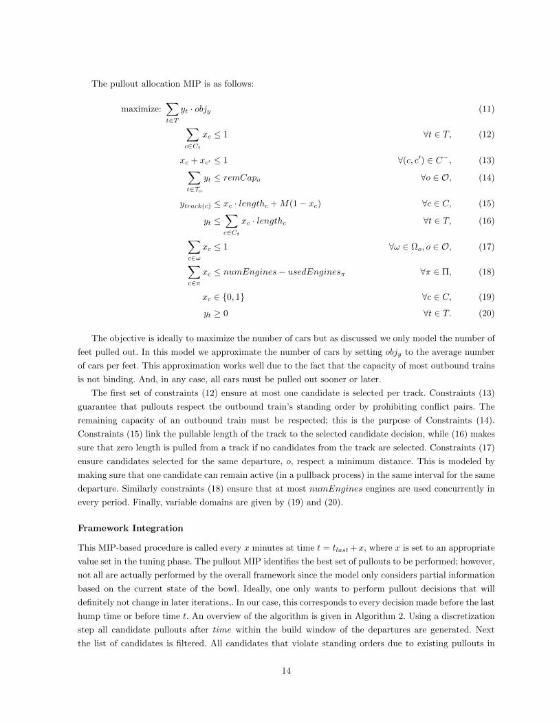
The pullout allocation MIP is as follows:

maximize:∑t∈T

yt · objy (11)∑c∈Ct

xc ≤ 1 ∀t ∈ T, (12)

xc + xc′ ≤ 1 ∀(c, c′) ∈ C−, (13)∑t∈To

yt ≤ remCapo ∀o ∈ O, (14)

ytrack(c) ≤ xc · lengthc +M(1− xc) ∀c ∈ C, (15)

yt ≤∑c∈Ct

xc · lengthc ∀t ∈ T, (16)

∑c∈ω

xc ≤ 1 ∀ω ∈ Ωo, o ∈ O, (17)∑c∈π

xc ≤ numEngines− usedEnginesπ ∀π ∈ Π, (18)

xc ∈ 0, 1 ∀c ∈ C, (19)

yt ≥ 0 ∀t ∈ T. (20)

The objective is ideally to maximize the number of cars but as discussed we only model the number of

feet pulled out. In this model we approximate the number of cars by setting objy to the average number

of cars per feet. This approximation works well due to the fact that the capacity of most outbound trains

is not binding. And, in any case, all cars must be pulled out sooner or later.

The first set of constraints (12) ensure at most one candidate is selected per track. Constraints (13)

guarantee that pullouts respect the outbound train’s standing order by prohibiting conflict pairs. The

remaining capacity of an outbound train must be respected; this is the purpose of Constraints (14).

Constraints (15) link the pullable length of the track to the selected candidate decision, while (16) makes

sure that zero length is pulled from a track if no candidates from the track are selected. Constraints (17)

ensure candidates selected for the same departure, o, respect a minimum distance. This is modeled by

making sure that one candidate can remain active (in a pullback process) in the same interval for the same

departure. Similarly constraints (18) ensure that at most numEngines engines are used concurrently in

every period. Finally, variable domains are given by (19) and (20).

Framework Integration

This MIP-based procedure is called every x minutes at time t = tlast+x, where x is set to an appropriate

value set in the tuning phase. The pullout MIP identifies the best set of pullouts to be performed; however,

not all are actually performed by the overall framework since the model only considers partial information

based on the current state of the bowl. Ideally, one only wants to perform pullout decisions that will

definitely not change in later iterations,. In our case, this corresponds to every decision made before the last

hump time or before time t. An overview of the algorithm is given in Algorithm 2. Using a discretization

step all candidate pullouts after time within the build window of the departures are generated. Next

the list of candidates is filtered. All candidates that violate standing orders due to existing pullouts in

14

the bowl are removed. Candidates that violate the separation constraint (of past assignments) on the

corresponding track are removed. Candidates that violate the separation constraint (of past assignments)

on the departure are also removed. The generated candidate pullout events and existing engine usage are

analyzed and the available engine capacity is stored for all relevant time periods.

Algorithm 2

1: procedure PulloutMIP(bowl, time, time’)2: C ← 3: for t ∈ ClassificationTracks do4: s ← FrontSegment(t, bowl, time)5: b ← BlockOfSegment(s)6: d ← DepartureOfBlock(b)7: (wα,wω) ← DepartureBuildWindow(d)8: C ← C∪ Filter(Generate(t,wα,wω))

9: model ← BuildMipModel(bowl, C)10: pullouts ← Solve(model)11: lastHump ← LastHumpedCar(bowl)12: for p ∈ pullouts do13: pt ← PulloutTime(p)14: if pt ≤ max(lastHump, time’) then15: bowl ← PerformPullout(bowl, p)

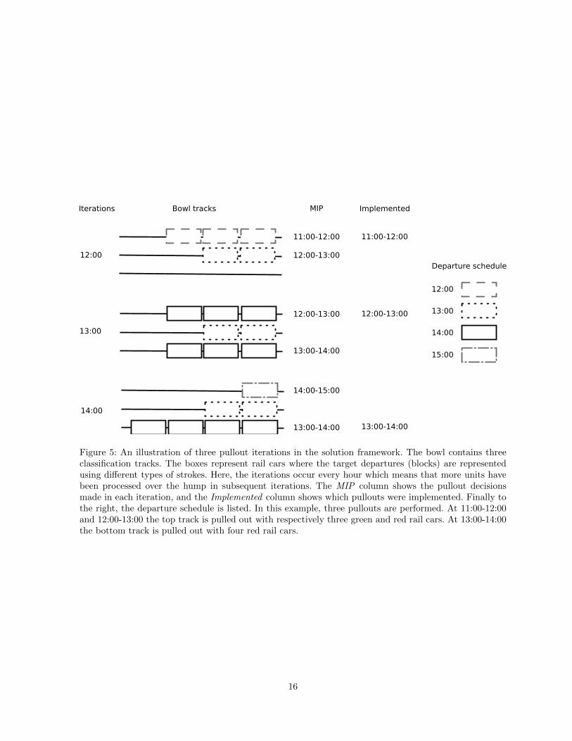
An example illustrating the pullout process in the solution framework is shown in Figure 5. For the

sake of argument we make a few simplifications. First, assume that every outbound train only has a

standing order of one block type. Second, assume that only one pullout engine exists and requires one

hour to perform one pullout. Third, assume that a outbound train can be built two hours in advance.

Finally, assume that all rail cars are of equal length. The example shows the relation between the decisions

made by the MIP (Algorithm 2) and the decisions actually implemented by the solution framework. Only

a subset of the the MIP decision are adopted by the framework as it only considers partial information.

Note, in Figure 5 at 12:00 the MIP recommends pulling two blue rail cars at 12:00-13:00 but in the next

iteration this decision has been changed (to pull three red rail cars instead) as more rail cars have arrived

in the bowl. Also note, in the second iteration, that the decision to pull three red rail cars at 13:00-14:00

is changed to pull four rail cars from the same track in the third iteration.

This approach is superior to the Greedy approach as it considers interdependencies between multiple

departures. Although the method operates on partial future information, depending on how much is in

the bowl, it can still consider future consequences of pullouts to some extent. Solving the MIP model

using a commercial solver allows us to find near optimal solutions very quickly in practice. This benefit

is, however, also a liability since the runtime overhead of using a general purpose solver must be paid.

The model has to be built and solved many times - in some cases building the model is more expensive

than solving it. For practical reasons, the number of generated candidates is limited or discretized, and

therefore the model is unable to gain a fine-grained control of the pullouts.

Finally, we mention that this approach assumes that only one line can be pulled out simultaneously.

The model should ideally consider the possibility of pulling multiple lines on a particular track; however,

given the limited number of lines allowed simultaneously in the bowl, this did not seem to be a critical

concern. The proposed model can be extended without much difficulty to handle multiple lines.

15

12:00

Departure schedule

13:00

Bowl tracks

14:00

15:00

Iterations MIP Implemented

11:00-12:00 11:00-12:00

12:00-13:0012:00

13:00

14:00

12:00-13:00 12:00-13:00

13:00-14:00

13:00-14:00

14:00-15:00

13:00-14:00

Figure 5: An illustration of three pullout iterations in the solution framework. The bowl contains threeclassification tracks. The boxes represent rail cars where the target departures (blocks) are representedusing different types of strokes. Here, the iterations occur every hour which means that more units havebeen processed over the hump in subsequent iterations. The MIP column shows the pullout decisionsmade in each iteration, and the Implemented column shows which pullouts were implemented. Finally tothe right, the departure schedule is listed. In this example, three pullouts are performed. At 11:00-12:00and 12:00-13:00 the top track is pulled out with respectively three green and red rail cars. At 13:00-14:00the bottom track is pulled out with four red rail cars.

16

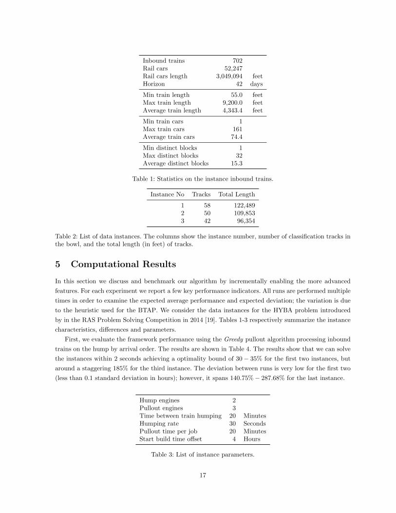
Inbound trains 702Rail cars 52,247Rail cars length 3,049,094 feetHorizon 42 days

Min train length 55.0 feetMax train length 9,200.0 feetAverage train length 4,343.4 feet

Min train cars 1Max train cars 161Average train cars 74.4

Min distinct blocks 1Max distinct blocks 32Average distinct blocks 15.3

Table 1: Statistics on the instance inbound trains.

Instance No Tracks Total Length

1 58 122,4892 50 109,8533 42 96,354

Table 2: List of data instances. The columns show the instance number, number of classification tracks inthe bowl, and the total length (in feet) of tracks.

5 Computational Results

In this section we discuss and benchmark our algorithm by incrementally enabling the more advanced

features. For each experiment we report a few key performance indicators. All runs are performed multiple

times in order to examine the expected average performance and expected deviation; the variation is due

to the heuristic used for the BTAP. We consider the data instances for the HYBA problem introduced

by in the RAS Problem Solving Competition in 2014 [19]. Tables 1-3 respectively summarize the instance

characteristics, differences and parameters.

First, we evaluate the framework performance using the Greedy pullout algorithm processing inbound

trains on the hump by arrival order. The results are shown in Table 4. The results show that we can solve

the instances within 2 seconds achieving a optimality bound of 30− 35% for the first two instances, but

around a staggering 185% for the third instance. The deviation between runs is very low for the first two

(less than 0.1 standard deviation in hours); however, it spans 140.75%− 287.68% for the last instance.

Hump engines 2Pullout engines 3Time between train humping 20 MinutesHumping rate 30 SecondsPullout time per job 20 MinutesStart build time offset 4 Hours

Table 3: List of instance parameters.

17

Dwell (hours)

No Time Arrival Bowl Departure Total Max Lines Gap

1.0 1.7 0.59 12.35 3.43 16.38 94.7 61.0 30.2%2.0 1.4 0.92 12.52 3.47 16.90 87.8 53.5 34.4%3.0 1.2 19.65 12.69 3.51 35.85 91.4 44.8 185.1%

Table 4: Results using a greedy humping and pullout strategy. The columns respectively show the instancenumber, average runtime in seconds, different average dwell time averages in hours, the average maximumno of concurrent lines in the bowl, and finally the relative optimality gap.

Dwell (hours)

No Time Arrival Bowl Departure Total Max Lines Gap

1.0 287 0.56 11.39 1.22 13.17 129.9 61.0 4.74%2.0 273 0.57 11.29 1.35 13.21 117.6 54.2 5.07%3.0 338 1.42 10.92 1.99 14.33 76.6 45.5 13.92%

Table 5: Results using a greedy humping method and the MIP pullout method. The columns respectivelyshow the instance number, average runtime in seconds, different average dwell time in hours, the averagemaximum no of concurrent lines in the bowl, and finally the relative optimality gap.

We do not see much improvement nor loss when activating low or high volume track selection for the

BTAP, mentioned in Section 4.3. Runtime remains unchanged, but a benchmark showed that only the

last data set is improved up to 2.4 average dwell hours.

The biggest improvement was observed when using the MIP method for the PAP instead of Greedy. The

results are summarized in Table 5. The benchmark reports a significant improvement in average/bound

for all instances. The last instance is, however, still around ten percentage points above the other two.

As expected, the runtime is increased, from a few seconds to a few minutes. A noticeable increase in

maximum dwell time can be observed compared to the previous benchmark, but the average maximum

number of lines is not changed significantly. This is to be expected since the MIP pullout approach does

not process the bowl on a first-come first-served fashion.

Finally we benchmark the performance of using the PAP MIP together with the HSP MIP method.

The results are shown in Table 6. A consistent improvement of 0.06 to 0.09 average hours was observed,

i.e., roughly 5000 dwell hours. It is observed that this setting improves the average dwell time at the bowl

and departure yards, while achieving a slightly increased dwell time at the arrival yard. The HSP MIP

method finds a better processing order of the arriving trains, at the cost of processing them more quickly

by arrival order. This improvement does, however, come at the cost of approximately twice the runtime.

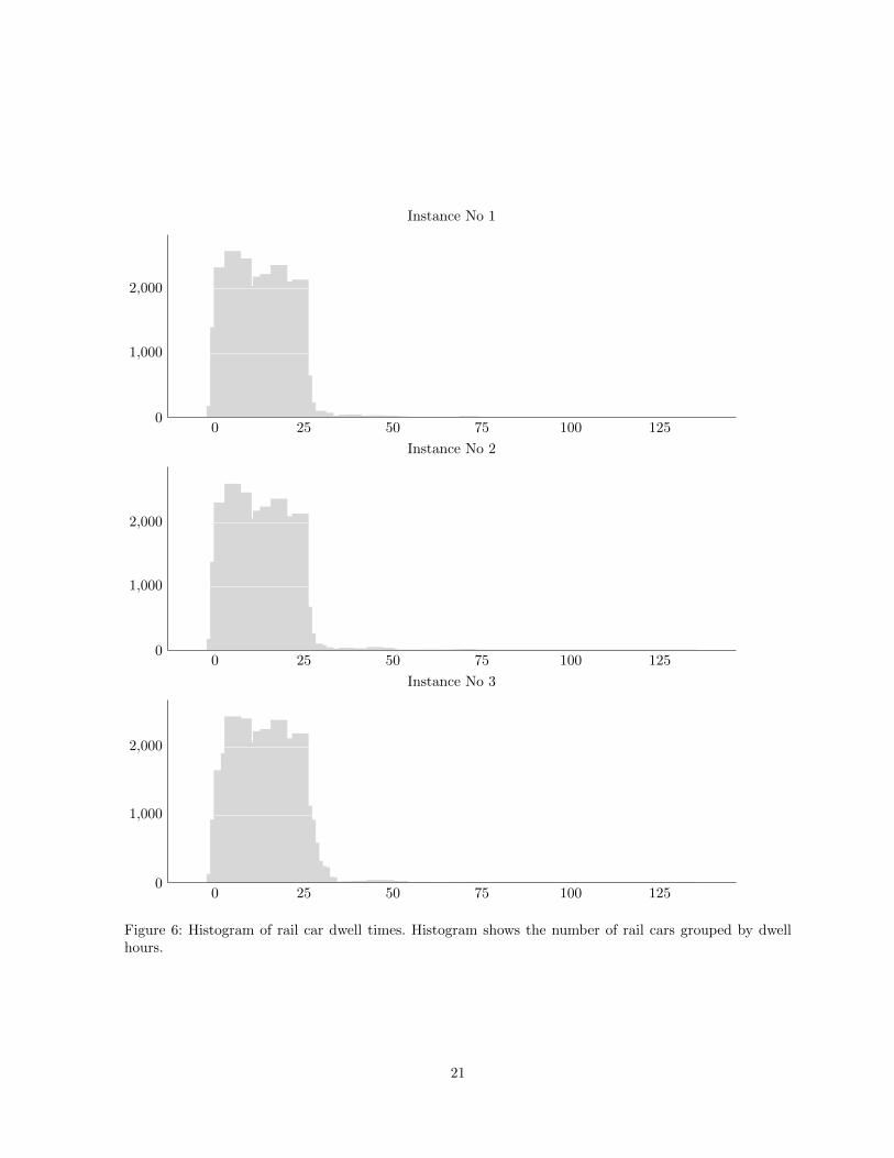
The maximum dwell time and average maximum line usage show no noticeable change. A histogram

showing the rail car dwell hour distribution, of one solution, is plotted in Figure 6. The majority of the

rail cars leave the yard within 25 hours of arrival. Very few rail cars stay in the yard more than 50 hours.

The solutions of all instances show a similar shape to Figure 6. Compared to the first two instances, the

last instance contains fewer rail cars with 0-5 hours dwell time and an increased number of rail cars with

more than 25 hours dwell time.

18

Time (s) Dwell (hours)

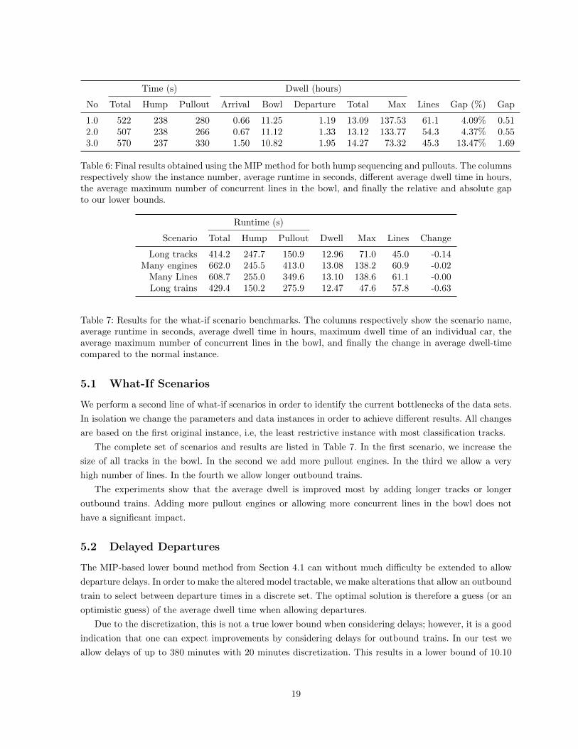
No Total Hump Pullout Arrival Bowl Departure Total Max Lines Gap (%) Gap

1.0 522 238 280 0.66 11.25 1.19 13.09 137.53 61.1 4.09% 0.512.0 507 238 266 0.67 11.12 1.33 13.12 133.77 54.3 4.37% 0.553.0 570 237 330 1.50 10.82 1.95 14.27 73.32 45.3 13.47% 1.69

Table 6: Final results obtained using the MIP method for both hump sequencing and pullouts. The columnsrespectively show the instance number, average runtime in seconds, different average dwell time in hours,the average maximum number of concurrent lines in the bowl, and finally the relative and absolute gapto our lower bounds.

Runtime (s)

Scenario Total Hump Pullout Dwell Max Lines Change

Long tracks 414.2 247.7 150.9 12.96 71.0 45.0 -0.14Many engines 662.0 245.5 413.0 13.08 138.2 60.9 -0.02

Many Lines 608.7 255.0 349.6 13.10 138.6 61.1 -0.00Long trains 429.4 150.2 275.9 12.47 47.6 57.8 -0.63

Table 7: Results for the what-if scenario benchmarks. The columns respectively show the scenario name,average runtime in seconds, average dwell time in hours, maximum dwell time of an individual car, theaverage maximum number of concurrent lines in the bowl, and finally the change in average dwell-timecompared to the normal instance.

5.1 What-If Scenarios

We perform a second line of what-if scenarios in order to identify the current bottlenecks of the data sets.

In isolation we change the parameters and data instances in order to achieve different results. All changes

are based on the first original instance, i.e, the least restrictive instance with most classification tracks.

The complete set of scenarios and results are listed in Table 7. In the first scenario, we increase the

size of all tracks in the bowl. In the second we add more pullout engines. In the third we allow a very

high number of lines. In the fourth we allow longer outbound trains.

The experiments show that the average dwell is improved most by adding longer tracks or longer

outbound trains. Adding more pullout engines or allowing more concurrent lines in the bowl does not

have a significant impact.

5.2 Delayed Departures

The MIP-based lower bound method from Section 4.1 can without much difficulty be extended to allow

departure delays. In order to make the altered model tractable, we make alterations that allow an outbound

train to select between departure times in a discrete set. The optimal solution is therefore a guess (or an

optimistic guess) of the average dwell time when allowing departures.

Due to the discretization, this is not a true lower bound when considering delays; however, it is a good

indication that one can expect improvements by considering delays for outbound trains. In our test we

allow delays of up to 380 minutes with 20 minutes discretization. This results in a lower bound of 10.10

19

average dwell hours. This significant reduction suggests that large savings can be achieved by allowing

departures to be delayed. We note that roughly half of all outbound trains were delayed in this lower

bound solution.

Finally, we benchmarked the result of allowing up to 2 hours delay in our solution methods, thus

getting a real solution instead of a bound. These settings generate average dwell hours of 12.31, 12.33,

and 12.42 the three datasets. Again, a significant improvement, especially for the last instance.

6 Conclusions

In this paper we consider the HYBA problem. We propose a heuristic framework which decomposes the

problem into three interdependent subproblems. A version of the algorithm in which we consider greedy

strategies for the humping and pullout process obtains acceptable solutions within two seconds. A second

version, in which the humping and pullout strategies are solved using MIP models, obtains solutions that

are significantly better; however, it does take substantially more time. The runtime is, however, still very

reasonable considering the length of the planning horizon. The solutions obtained have a proven optimality

gap of a few percent. An additional experiment shows that significant improvements can be obtained by

allowing outbound trains to be delayed.

In addition to solving the HYBA problem the proposed heuristic method can be used to estimate the

effect of infrastructure or equipment investments. Several what-if scenarios are considered and the results

show that the studied data instance can benefit from longer outbound trains and additional track-length

in the classification yard. However, allowing more concurrent lines in the bowl or using additional pullout

engines does not make a significant difference.

Simple methods have been proposed for finding lower bounds for the problem. The results show that

the lower bounds give good estimates for the two first instances. The methods do not take the bowl tracks

into account, which explains why a weaker bound is achieved for the last instance. Promising directions

for future research include strengthening this lower bound calculation to reflect the limitations of fewer

bowl tracks as well as integrating certain components of the algorithm. In particular, one idea could be to

allocate a set of rail cars to bowl tracks when humping a specific car, as opposed to the current approach

of greedily allocating each individual rail car a track when it is being humped. Finally, having the ability

to dynamically adjust the humping sequence may also yield further improvements.

References

[1] R.K. Ahuja, K.C. Jha, and J. Liu, Solving real-life railroad blocking problems, Interfaces 37 (2007),

404–419.

[2] L.D. Bodin, B.L. Golden, A.D. Schuster, and W. Romig, A model for the blocking of trains, Trans-

portation Res Part B: Methodological 14 (1980), 115 – 120.

[3] M. Bohlin, F. Dahms, H. Flier, and S. Gestrelius, Optimal freight train classification using column

generation, ATMOS, Vol. 25 of OASICS, Schloss Dagstuhl - Leibniz-Zentrum fuer Informatik, 2012,

pp. 10–22.

20

0 25 50 75 100 1250

1,000

2,000

Instance No 1

0 25 50 75 100 1250

1,000

2,000

Instance No 2

0 25 50 75 100 1250

1,000

2,000

Instance No 3

Figure 6: Histogram of rail car dwell times. Histogram shows the number of rail cars grouped by dwellhours.

21

[4] M. Bohlin, F. Dahms, and S. Gestrelius, Optimisation of simultaneous train formation and car sorting

at marshalling yards, Report 2013–013, Operations Research, RWTH Aachen University, Jul 2013.

[5] M. Bohlin, S. Gestrelius, F. Dahms, M. Mihalak, and H. Flier, Optimized shunting with mixed-usage

tracks, Technical report 2013-12-19, Swedish Institute of Computer Science, 2013.

[6] N. Boysen, M. Fliedner, F. Jaehn, and E. Pesch, Shunting yard operations: Theoretical aspects and

applications, Eur J Oper Res 220 (2012), 1 – 14.

[7] D. Briskorn and F. Jaehn, A note on “Multistage methods for freight train classification”, Networks

62 (2013), 80–81.

[8] E. Dahlhaus, P. Horak, M. Miller, and J.F. Ryan, The train marshalling problem, Discr Appl Math

103 (2000), 41 – 54.

[9] J.R. Dirnberger and C.P.L. Barkan, Lean railroading for improving railroad classification terminal

performance: Bottleneck management methods, Transportation Res Record: J Transportation Res

Board 1995 (2007), 52 – 61.

[10] M. Gatto, J. Maue, M. Mihalak, and P. Widmayer, “Shunting for dummies: An introductory algo-

rithmic survey,” Robust and online large-scale optimization, R. Ahuja, R. Mohring, and C. Zaroliagis

(Editors), Springer, 2009, Vol. 5868 of Lecture Notes in Computer Science, pp. 310–337.

[11] S. He, R. Songa, and S.S. Chaudhry, An integrated dispatching model for rail yards operations,

Comput & Oper Res 30 (2003), 939 – 966.

[12] R. Jacob, P. Marton, J. Maue, and M. Nunkesser, Multistage methods for freight train classification,

Proc 7th Workshop Algorithmic Approaches Transportation Modeling, Optim, Syst (ATMOS’07),

Schloss Dagstuhl, Internationales Begegnungszentrum fur Informatik, Nov 2007, pp. 158–174.

[13] E.R. Kraft, Priority-based classification for improving connection reliability in railroad yards. part I

of II: Integration with car scheduling, Transportation Res Forum (2002), 93–105.

[14] E.R. Kraft, Priority-based classification for improving connection reliability in railroad yards. part II

of II: Dynamic block to track assignment, Transportation Res Forum (2002), 107–119.

[15] E. Lin and C. Cheng, Yardsim: A rail yard simulation framework and its implementation in a major

railroad in the U.S., Winter Simulation Conference, WSC, 2009, pp. 2532–2541.

[16] E. Lin and C. Cheng, Simulation and analysis of railroad hump yards in North America, Winter

Simulation Conference, WSC, 2011, pp. 3715–3723.

[17] J. Maue, On the problem of sorting railway freight cars: An algorithmic perspective, Ph.D. Thesis,

ETH Zurich, Gottingen, Germany, July 2011.

[18] H.N. Newton, C. Barnhart, and P.H. Vance, Constructing railroad blocking plans to minimize han-

dling costs, Transportation Sci 32 (1998), 330–345.

22

[19] Railway Applications Section, Institute for Operations Research and the Management Sciences (IN-

FORMS), Railroad hump yard block-to-track assignment, webpage. www.informs.org/Community/

RAS.

23