A MATHEMATICAL MODEL FOR -PHASE SPECIFIC -PHASE AND ...

MATHEMATICAL BIOSCIENCES http://www.mbejournal.org/AND ENGINEERINGVolume 4, Number 2, April 2007 pp. 239–259

A MATHEMATICAL MODEL FOR M-PHASE SPECIFICCHEMOTHERAPY INCLUDING THE G0-PHASE AND

IMMUNORESPONSE

Wenxiang Liu

Department of Mathematical & Statistical Sciences, University of AlbertaEdmonton, T6G 2G1, Canada

Thomas Hillen


H. I. Freedman


(Communicated by Yang Kuang)

Abstract. In this paper we use a mathematical model to study the effect ofan M -phase specific drug on the development of cancer, including the restingphase G0 and the immune response. The cell cycle of cancer cells is split intothe mitotic phase (M-phase), the quiescent phase (G0-phase) and the inter-phase (G1, S, G2 phases). We include a time delay for the passage through theinterphase, and we assume that the immune cells interact with all cancer cells.We study analytically and numerically the stability of the cancer-free equilib-rium and its dependence on the model parameters. We find that quiescentcells can escape the M -phase drug. The dynamics of the G0 phase dictatesthe dynamics of cancer as a whole. Moreover, we find oscillations through aHopf bifurcation. Finally, we use the model to discuss the efficiency of cellsynchronization before treatment (synchronization method).

1. Introduction. Chemotherapy treatment has demonstrated a definite capacityfor controlling disseminated metastatic cancer and is widely used. Unfortunately,drugs in cancer chemotherapy kill normal as well as cancerous cells. Naturally it isdesirable to kill as many cancerous cells as possible while sparing as many normalcells as possible. One way of accomplishing this goal is by taking advantage of thefact that many chemotherapeutic drugs are cycle-specific: they destroy cells only inspecific phases of the cells’ cycle. In the cell synchronization method, the cancerouscells are first synchronized by one drug. When nearly all the cancerous cells reachthe desirable phase, they are treated with a second, cycle-specific drug. This killsthe maximum number of cancer cells while sparing large numbers of normal cells.Some examples of such drugs are Cytosine Arabinoside (Ara-C), 5-fluorouracil andPrednisone, which work in the G1 and S phases of the cell-cycle, and Vincristine,Paclitaxel and Bleomycin which work in the M phase of the cell-cycle [9, 15]. The

2000 Mathematics Subject Classification. 92B05.Key words and phrases. cycle-phase-specific drugs, time delay, cancer growth, Hopf

bifurcation.

239

240 W. LIU, T. HILLEN AND H. I. FREEDMAN

cell is blocked from continuing in the cell cycle, and thus the drugs stop the cellproliferation and allow the immune system to attack and kill cancerous cells in anatural way [27].

A classical cell cycle model, the G0-model, has been developed by Mackey [18].Examples of the more recent work done with mathematical models of cycle-specificchemotherapy are by Webb [28] and Kheifetz et al. [12]. They develop linear andnonlinear age-structured models of cycle-specific chemotherapy. The advantage ofshorter dosage periods are investigated in the case of the linear model. Anotherwork of interest is by Birkhead et al. [1], in which a four-compartment linear sys-tem is developed to model the cycling, resistant and resting cells. Their results arelimited to a few numerical calculations on four specific types of treatments. Swan[25] also examines cycle-specific chemotherapy in his review article. Particularly, heconcentrates on age-structured models that take into account the age of the cells ineach compartment of the cell cycle. He also studies an age-structured chemother-apeutic model of acute myeloid leukemia. The fact is that in the above articlesonly chemotherapy, not immunoresponse, is considered. Kirschner and Panetta[14] include the immune system in a mathematical model to study immunotherapyas an alternative to chemotherapy. In [27] Villasana and Radunskaya model thecycle-specific chemotherapy that includes the immune system but excludes the rest-ing stage. In their paper, they study the interaction of tumor cells and drug withthe immune system and show that the stability of fixed points may depend on thedelay. De Boer at al. [7] represent a more specific model to study the macrophageT lymphocyte interactions that generate an antitumor immune response. Withrespect to cancer interaction with immune cells, the main difference between ourwork and theirs is that in their case they study a very specific type of lymphocytewhich interacts with tumor cells, while in our case we consider a more general typeof immune cells with main focus on the cycle-specificity of M-phase chemotherapy.

With respect to cancer interaction with immune cells, DeLisi and Resoigno [8]employ a simple deterministic predator-prey model to simulate immune surveillancein which immune cells and molecules are stimulated by a transplanted tumor. Aspecific model for T lymphocyte response to the growth of an immunogenic tumoris given by Kuznetsov et al. [17]. The model is used to describe the kinetics ofB-lymphoma BCL1 in the spleen of mice. Moreover, the model is applied to theanalysis of immuno-stimulation of tumor growth, formation of a tumor dormancyand sneaking through of the tumor. With respect to growth kinetics of immunecells we use a model similar to that of Kuznetsov et al. [17]. With respect tocancer interaction with cycle-specific drugs, Kozusko et al. [16] develop a mathe-matical model to study the in-vitro cancer cell growth and response to treatmentwith the experimental antimitotic agent curacin A. They predict that curacin Awill be quickly absorbed into cell phases and will express an effective control ofcancer growth; that is, the cells will response with an increase in the rate of DNAsynthesis, a decrease in the rate of mitosis and possibly an increase in the rateof apoptosis. In [4] Cojocaru and Agur provide a formal method for predictingthe effect on treatment efficacy of cell-cycle-specific drugs, such as the cancer drugcytosine arabinoside (Ara-C). A comprehensive review of recent relevant results inmathematical modeling and control of the cell cycle and of the mechanisms of geneamplification (related to drug resistance), and estimation of the constructed modelsis given by Kimmel and Swierniak [13].

CHEMOTHERAPY AND G0-PHASE 241

Table 1. Variables in model system

variable meaning unitx number of cancer cells in the interphase cellsy number of cancer cells in the mitotic phase cellsz number of cancer cells in the resting phase cellsI number of lymphocytes cellsu biomass of chemotherapy drugs mg

The model we propose is an extension of the models above, in particular with re-spect to the quiescent G0-phase. Our analysis shows that the G0-phase is a criticalfactor for cancer treatment. Our model is based on a model the model developedby Villasana and Radunskaya [27]. However, we find that the model in [27] is ques-tionable in the development of one of the model’s delay terms, which will makesolutions of the system negative in positive time. Therefore, we modify their modeland include the immune system and the quiescent stage into the model. The mainconclusion from our analysis is that a resting phase of tumor cells is the most im-portant compartment for cancer treatment with an M -phase specific drug. Thisconfirms the general understanding that cancer cells can avoid the chemotherapeu-tic agent in the resting compartment (see, for example, www.cancerhelp.org.uk).The surviving quiescent cells can contribute to further tumor growth when thechemotherapeutic effect has failed. For the analysis, here we study a single drugdose at time t = 0 only. However, in the numerical simulations, we also study mul-tiple dosage protocols and find that multiple dosage protocols do not change thequalitative result. Thus the resting cells are the limiting factor for chemotherapy(according to our model). Additionally, we find that a time delay for the interphasecan lead to stability switches. One implication is a scenario, where cancer cells canbe controlled by arresting cells in the interphase. In these cases the arrested cellsare subsequently killed by the immune response. In any case, the M -phase specificdrug certainly reduces the overall tumor load of a patient, even though it mightnot cure cancer alone.

We present and develop the new model in section 1.1, whereas in section 1.2 wecarry out a nondimensionalization to reduce the number of parameters.

The active cell compartment includes a time delay related to the transition ofcells through the G1, S and G2 phases. We split our analysis according to this delay,studying the no-delay case in section 2 and the delay case in section 3. In both caseswe investigate the stability of the cancer-free equilibrium in the cases of (i) no drugand no immune response, (ii) immune suppression without drug, and (iii) immunesuppression with drug. In all cases we show that adminstration of an M-phasespecific drug does not change the stability of the cancer-free equilibrium. However,cancer growth is significantly reduced by the drug, and in the case of a delay thedrug can initiate or destroy oscillations. We prove a corresponding result on Hopfbifurcation in section 3.4. Moreover, in the delay case we prove the existence ofa stability switch if the delay parameter is beyond a certain value. Furthermore,adminstration of an M-phase specific drug can lead to partial cell synchronization(expressed through oscillating solutions). In section 4, we illustrate our results withnumerical simulations. The paper closes with a discussion in section 5.


7

G

δ3

k3

τ

δ4κ

0

+S+G2G1 Mδ2

γ

u

I

k

k

k k

4

5

1 2

k

kδ1

α α

α

23

1

6

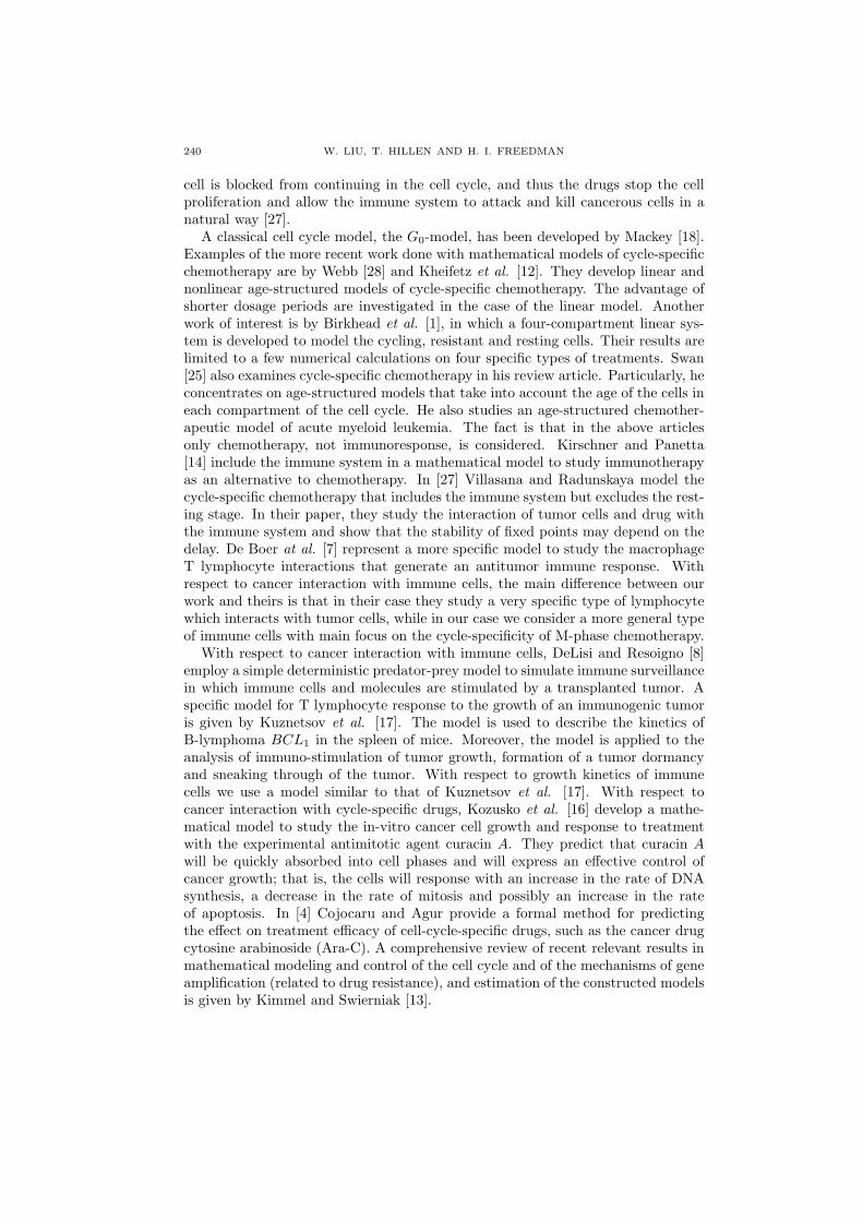
Figure 1. Arrow diagram of the cell cycle model (1) indicatingimmune response, I, and M-phase -specific drug, u.

1.1. The model. We take as our model of cancer treatment by chemotherapy asystem of delayed differential equations, which takes the form

x(t) = α3z(t)︸︷︷︸from resting phases

− α1x(t)︸︷︷︸flowing into mitosis phases

− δ1x(t)︸︷︷︸natural death

− k1I(t)x(t)︸︷︷︸destroyed by lymphocytes

y(t) = α1x(t− τ)︸︷︷︸from interphases

− α2y(t)︸︷︷︸to resting phases

− δ2y(t)︸︷︷︸natural death

− k2I(t)y(t)︸︷︷︸destroyed by lymphocytes

− k4(1− e−k5u(t))y(t)︸︷︷︸destroyed by drugs

z(t) = 2α2y(t)︸︷︷︸from mitosis

− α3z(t)︸︷︷︸to reproduce

− δ3z(t)︸︷︷︸natural death

− k3I(t)z(t)︸︷︷︸destroyed by lymphocytes

I(t) = k︸︷︷︸constant growth source

+ρI(t)(x + y + z)n

a + (x + y + z)n

︸︷︷︸growth due to stimulus

− δ4I(t)︸︷︷︸natural death

− (c1x(t) + c2y(t) + c3z(t))I(t)︸︷︷︸combined with cancer cells

− k6(1− e−k7u(t))I(t)︸︷︷︸destroyed by drugs

u(t) = −γu(t)︸︷︷︸exponential decay

,

with initial conditions

x(t) = φ1(t), t ∈ [−τ, 0] , y(0) = y0, z(0) = z0, I(0) = I0, u(0) = u0.

A schematic of this model is given in Figure 1, the meaning of each variable is listedin Table 1, and the interpretation of parameters is given in Table 2.


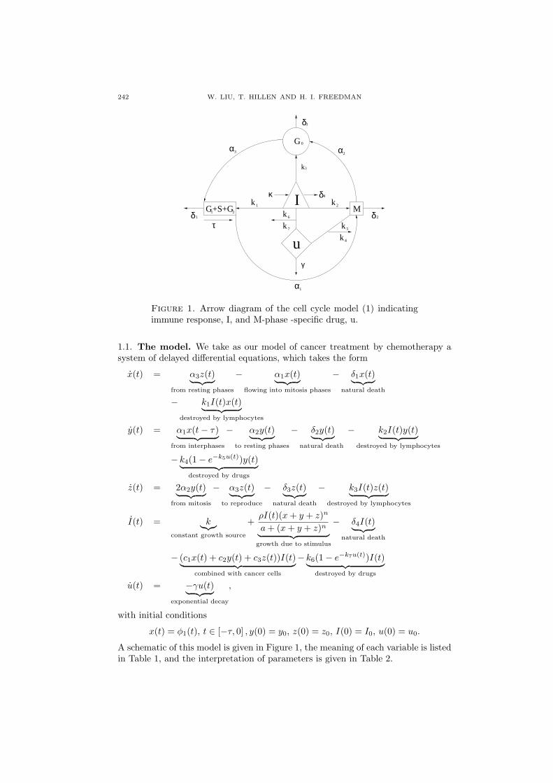
Table 2. Parameters in the model system

parameter meaning value ref.

α1 rate at which cells flow into the mi-tosis phase

0− 1/day [18, 27]

α2 rate at which cells flow into the rest-ing phase

0− 1/day [18]

α3 rate at which cells leave from theresting phase to enter the cycle toreproduce

0− 1/day [18]

ci(i = 1, 2, 3) losses due to the encounters withimmune cells

0.01× 10−6 − 1×10−6/cell day

[17, 27]

δi(i = 1, 2, 3) proportions of natural death of x, y,and I

0− 1/day [17, 27]

δ3 rate at which cells leave from theresting state to enter the blood

0− 0.056/day [18, 24]

ρ proportion of the growth of lympho-cytes due to stimulus by cancer cells

0.2/day [14, 27]

a speed at which the lymphocytesreach saturation level without stim-ulation

0.5 × (0.1 ×106cell)3

[14, 27]

k growth rate of the lymphocytes inthe absence of cancer cells

0.15×106cell/day [17, 27]

ki(i = 1, 2, 3) rates at which lymphocytes destroycells in different phases

0.1 × 10−8 − 1 ×10−8/cell day

[17, 27]

ki (i = 4, 6) proportions of drugs which elimi-nate cancer cells and lymphocytes

0− 1/day [22, 27]

ki (i = 5, 7) proportions of drugs which elimi-nate cancer cells and lymphocytes

0.01× 10−2 − 1×10−2/mg

[[27]

γ proportion of decay of the drugs 0.1 × 10−2 − 1 ×10−2/day

[27]

τ resident time of cells in the inter-phase

0− 2 days [18, 27]

All constants are positive. By and large, cancer cells cannot differentiate intomaturer forms of precursors. Consequently, we assume here that the cancer cellsbehave as a proliferative pool only. The cancer cells are self-renewing and consist ofa resting compartment and an active compartment that is split into four phases dueto cycle-specificity consideration here. In the resting state, the cancer cells leave atrandom to enter either the active compartment or the blood at fractional rates α3

and δ3. Cells in the blood are largely nonproliferative, and they are for the mostpart destined to die [23]. For the cancer population we consider here, stem cellinflux is assumed to be negligible. The cancer cells reside in the cycle for a certainperiod of time τ before entering into the mitotic stage. Thus we have the termx(t− τ) in the system. The corresponding model in [27] has a negative delay term−αx(t− τ) in the x-equation. This is problematic, because solutions might becomenegative and unphysiological oscillations occur. Besides the modified term −αx(t),our model includes the resting phase explicitly (z-equation), which was not studiedin [27]. The terms δ1x(t), δ2y(t), δ3z(t), δ4I(t) in the model equations representproportions of natural cell death or apoptosis, α1, α2 and α3 represent the differentrates at which cells flow between different phases or reproduce, the terms ki and


ci (i = 1, 2, 3) represent losses from encounters of cancer cells with lymphocytes.We model the interaction of immune cells with cancer by the law of mass action.With respect to immune response function, the term ρI(t)(x(t)+y(t)+z(t))n

a+(x(t)+y(t)+z(t))n representsthe nonlinear growth of the immune population due to stimulus by the cancer cells.Here we have chosen a Michaelis-Menten form for this term, following the literature(see, for example, [14, 17, 27]). We think it is reasonable, because proliferation ofcancer-specific effector cells is stimulated by the presence of cancer cells but reachesa saturation level at cancer population. The saturation level depends on the healthof the immune system, specifically on its ability to produce certain cytokines. Inthe absence of cancer cells (x = y = z = 0), the immune cells grow at a constantsource rate k. Therefore, the recruitment function should be zero when there areno cancer cells and should increase monotonically toward a horizontal asymptote;this rational form reflects these characteristics in a simple, smooth function. Theparameters ρ, a and n depend on the type of cancer being considered. With respectto high densities of drugs, we know that the drug interferes with cancer cells inmitosis, causing them to die naturally when they fail to complete the cycle [27].Therefore we assume that once the drug encounters the cancer cell, the cancer cellis taken out of the cycle and can no longer proliferate. This is modeled by the term−k4(1 − e−k5u)y [4, 27], but there are other curves that describe a similar feature(see [22]). The drug decay is assumed to be exponential , and the coefficient γincorporates both the elimination and absorption effects [27]. In [26] the effect ofmultiple applications of the drug is considered. Here we focus on a single drug dosetreatment only. Multiple dosage protocols and other treatment options are beyondthe scope of this paper. We also assume that the drug is harmful to the immunesystem and we leave a similar term in the I(t) equation. Biologically, this treatmentterm means that when no drugs are applied (k5 = 0), there are no effects on thecancer cell population, since 1− e−k5u = 0. Further, k4 represents the intensity ofthe treatment. In this new model, we assume that the resting cells are not affectedby the drugs but immune cells will attack them. This assumption derives from thefact that faster proliferating cells are more sensitive to the drugs, while the cells inthe resting phase escape the action of cycle-specific cytotoxic agents [27]. For otherassumptions for the model, the reader is referred to [27].

1.2. Nondimensionalization. As in [27], we nondimensionalize the system andwrite

t =t

day, x =

x

x(0), y =

y

x(0), z =

z

z(0), I =

I

I(0), u =

u

u(0), s =

z(0)x(0)

,

k1 = k1I(0), k2 = k2I(0), k3 = k3I(0), k5 = k5u(0), k7 = k7u(0),

a = a/xn(0), c1 = c1x(0), c2 = c2x(0), c3 = c3z(0), k = k/I(0),

where x(0) = y(0) are initial values. By renaming the variables t, x, y, z, I , u tot, x, y, z, I, u respectively and the parameter values k, a, ki, cj to k, a, ki, cj respec-tively, i = 1 − 7; j = 1 − 3. Then, none of the new parameters and variables have


dimensions. From this point on we will work with the nondimensionalized model:

x(t) = sα3z(t)− α1x(t)− (δ1 + k1I(t))x(t)y(t) = α1x(t− τ)− (α2 + δ2 + k2I(t))y(t)− k4(1− e−k5u(t))y(t)z(t) = 2s−1α2y(t)− (α3 + δ3 + k3I(t))z(t)I(t) = k + ρI(t)(x+y+sz)n

a+(x+y+sz)n − (δ4 + c1x(t) + c2y(t) + c3z(t))I(t)−k6(1− e−k7u(t))I(t)

u(t) = −γu(t),

(1)

with initial conditions

x(t) = φ1(t), t ∈ [−τ, 0] , y(0) = y0 , z(0) = z0 , I(0) = I0 , u(0) = u0.

2. Stability results for the nondelay case. We first determine the type ofdynamics that can arise in the system without the presence of the delay and thenstudy the case with delay in section 3. A summary of the stability results appearsin the discussion section, table 3. We begin by analyzing the simplest case: adrug-free model in a nondelay situation in the absence of an immune response.

2.1. Drug-free model in the absence of an immune response. In this sub-section, we shall study the drug-free model in a nondelay case without an immuneresponse. Necessary and sufficient conditions that guarantee the stability of thecancer-free equilibrium are obtained. Also, a necessary condition for cancer growthis obtained. In this case the equations are a simple set of ordinary differentialequations:

x(t) = −(α1 + δ1)x(t) + sα3z(t)y(t) = α1x(t)− (α2 + δ2)y(t)z(t) = 2s−1α2y(t)− (α3 + δ3)z(t),

(2)

with initial valuesx(0) = x0, y(0) = y0, z(0) = z0.

This is a linear system with the only equilibrium being E0(0, 0, 0). The Jacobianmatrix about this equilibrium is

−(α1 + δ1) 0 sα3

α1 −(α2 + δ2) 00 2s−1α2 −(α3 + δ3)

,

and the characteristic equation is

λ3 + a2λ2 + a1λ + a0 = 0,

wherea2 = α1 + δ1 + α2 + δ2 + α3 + δ3

a1 = (α1 + δ1)(α2 + δ2) + (α2 + δ2)(α3 + δ3) + (α3 + δ3)(α1 + δ1)a0 = (α1 + δ1)(α2 + δ2)(α3 + δ3)− 2α1α2α3

= α1α2(δ3 − α3) + (α3 + δ3)(α1δ2 + α2δ1 + δ1δ2).

(3)

Clearly, a2, a1 are positive and a2a1 > a0. By the Routh-Hurwitz criteria [6],necessary and sufficient conditions for λ to have negative real parts become a0 > 0.

As a result, we have the following lemma.

Lemma 2.1. The cancer-free equilibrium E0 of system (2) is locally asymptoticallystable if and only if a0 > 0.


Biomedical interpretationNote that G0 acts as a control center to determine the rate of proliferation. α3

represents the release rate at which cells in the resting phase at random enter intotheir cell cycles to reproduce cells, and δ3 is the fractional rate at which cells arereleased randomly into the blood from the resting phase.

Assume a0 > 0 such that a cancer is growing. To control the cancer growth andgive a biomedical interpretation of this first result, we consider parameters that arebeneficial for cancer eradication. In Lemma 1 the only condition for cancer decayis a0 > 0. Hence for cancer to grow, a necessary condition is α3 > δ3, which meansthat the rate, δ3, of leaving the resting state G0 must be smaller than the transitionrate α3 from the resting compartment to the active compartment. If δ3 > α3 cancerwill not grow (according to this model). It is interesting that already in this simplemodel the quiescent compartment G0 controls the cancer dynamics. This fact willbe confirmed by the more complex models later and has also been identified forradiation treatment in Dawson and Hillen [10].

2.2. Drug-free model in the presence of immune suppression. In this sub-section, we will add the effect of immune suppression to study how lymphocyteswill change the dynamical behavior of cancer cells when τ = 0. New conditions forcancer growth or extinction that involve the immune suppression parameter termswill be obtained. When adding immune suppression, the system becomes

x(t) = −(α1 + δ1)x(t) + sα3z(t)− k1x(t)I(t)y(t) = α1x(t)− (α2 + δ2)y(t)− k2y(t)I(t)z(t) = 2s−1α2y(t)− (α3 + δ3)z(t)− k3z(t)I(t)I(t) = k + ρI(t)(x+y+sz)n

a+(x+y+sz)n − (c1x(t) + c2y(t) + c3z(t) + δ4)I(t).

(4)

Note that E1(0, 0, 0, k/δ4) is an equilibrium of this system with zero cancer level anda positive immune level. In general, there will be other fixed points, but this fixedpoint is of particular interest since it represents a cancer-free state. The Jacobianmatrix about E1 is

−(α1 + δ1 + k1kδ4

) 0 sα3 0α1 −(α2 + δ2 + k2k

δ4) 0 0

0 2s−1α2 −(α3 + δ3 + k3kδ4

) 0− c1k

δ4− c2k

δ4− c3k

δ4−δ4

.

Clearly, λ = −δ4 is an eigenvalue, and the remaining eigenvalues are given by thesolutions to the characteristic equation

λ3 + b2λ2 + b1λ + b0 = 0, (5)

whereb2 = α1 + δ1 + α2 + δ2 + α3 + δ3 + k

δ4(k1 + k2 + k3)

b1 = (α1 + δ1 + k1kδ4

)(α2 + δ2 + k2kδ4

) + (α2 + δ2 + k2kδ4

)(α3 + δ3 + k3kδ4

)+ (α3 + δ3 + k3k

δ4)(α1 + δ1 + k1k

δ4)

b0 = (α1 + δ1 + k1kδ4

)(α2 + δ2 + k2kδ4

)(α3 + δ3 + k3kδ4

)− 2α1α2α3

= α1α2(δ3 + k3kδ4− α3) + (α3 + δ3 + k3k

δ4)(α1α2

+ α1(δ2 + k2kδ4

) + α2(δ1 + k1kδ4

) + (δ1 + k1kδ4

)(δ2 + k2kδ4

)).

(6)

Obviously, b2, b1 are positive and b2b1 > b0. By the Routh-Hurwitz criteria [6],necessary and sufficient conditions for λ to have negative real parts become b0 > 0.


As a result, we have the following.

Lemma 2.2. For system (4), the equilibrium E1 is locally asymptotically stable ifand only if b0 > 0.

Biomedical interpretationNote that b0 ≥ a0. Hence even if without immune response a cancer grows

(a0 < 0), an immune response can be able to control cancer growth. In our modelthis occurs for example if α3 > δ3 and k3k

δ4> α3−δ3. The parameter k represents the

growth rate of lymphocytes, k3 represents the rate at which lymphocytes destroy thecancer cells in the resting phase, and δ4 is the the natural death rate of lymphocytesin the resting compartment.

In certain circumstances an increase in the number of lymphocytes might even-tually increases the chance of cancer survival. This occurs if b0 ≤ 0, which impliesthat cancer cells outgrow the immune response (α3 > δ3 + kk3

δ4). This behavior has

in fact been observed by Prehn [23].

2.3. Drug model with immune suppression. Now we shall begin to considerthe effect of an M-phase specific drug in the model along with the immune sup-pression when there is no delay, τ = 0. We are interested in studying how theconditions for the cancer growth or extinction are varied when we apply drugs tothe model. In this case the system considered becomes

x = −(α1 + δ1)x + sα3z − k1xIy = α1x− (α2 + δ2)y − k2yI − k4(1− e−k5u)yz = 2s−1α2y − (α3 + δ3)z − k3zI

I = k + ρI(x+y+sz)n

a+(x+y+sz)n − (c1x + c2y + c3z + δ4)I − k6(1− e−k7u)Iu = −γu.

(7)

Under these circumstances, E2(0, 0, 0, k/δ4, 0) is an equilibrium of this system withzero cancer and drug levels and a positive immune level. Again, in general there areother fixed points, but this fixed point is of particular interest since it represents acancer and drug-free state. The Jacobian matrix about E2 is

−(α1 + δ1 + k1kδ4

) 0 sα3 0 0α1 −(α2 + δ2 + k2k

δ4) 0 0 0

0 2s−1α2 −(α3 + δ3 + k3kδ4

) 0 0− c1k

δ4− c2k

δ4− c3k

δ4−δ4

k6k7kδ4

0 0 0 0 −γ

.

Clearly, λ = −γ, λ = −δ4 are two eigenvalues. The remaining eigenvalues are thesame as the solutions to characteristic equation (5); that is,

λ3 + b2λ2 + b1λ + b0 = 0,

where b2, b1, b0 are given by (6) in section 2.2. Using the same argument seen insection 2.2, we have the following lemma.

Lemma 2.3. For system (7), the cancer-free equilibrium E2 is locally asymptoticallystable if and only if b0 > 0.

Summary for the nondelay caseComparing with Lemma 2 in section 2.2, Lemma 3 shows that the condition for

the extinction of cancer cells in all phases remains the same, which implies that


the drug does not have any effects on the stability of the cancer-free equilibrium.This is because the cancer cells in the resting phase escape the action of the cycle-specific cytotoxic agents, and the drug was only given once. A numerical examplefor multiple dosages is given Figure 4. Therefore, we have the following.

(i) We find that including immune suppression in the model greatly helps tostabilize the system and inhibit the further growth of cancer cells (see the first termof b0). This is reasonable, because some cancer cells are destroyed by lymphocytes,and increasing a0 in terms of lymphocyte parameters makes conditions less favorablefor cancer survival.

(ii) It follows from Lemma 2 that in certain situations lymphocytes lose theability to recognize these cancer cells, and the cancer cells will continue to reproduceat a larger rate and eventually dominate the normal tissues.

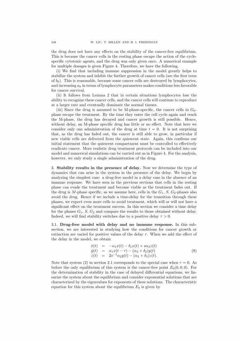
(iii) Since the drug is assumed to be M-phase-specific, the cancer cells in G0-phase escape the treatment. By the time they enter the cell cycle again and reachthe M-phase, the drug has decayed and cancer growth is still possible. Hence,without delay, an M-phase specific drug has little or no effect. Note that here weconsider only one administration of the drug at time t = 0. It is not surprisingthat, as the drug has faded out, the cancer is still able to grow, in particular ifnew viable cells are delivered from the quiescent state. Again, this confirms ourinitial statement that the quiescent compartment must be controlled to effectivelyeradicate cancer. More realistic drug treatment protocols can be included into ourmodel and numerical simulations can be carried out as in Figure 4. For the analysis,however, we only study a single administration of the drug.

3. Stability results in the presence of delay. Now we determine the type ofdynamics that can arise in the system in the presence of the delay. We begin byanalyzing the simplest case: a drug-free model in a delay case in the absence of animmune response. We have seen in the previous sections that cells in the restingphase can evade the treatment and become viable as the treatment fades out. Ifthe drug is M -phase specific, as we assume here, cells in the G1, S, G2-phases alsoavoid the drug. Hence if we include a time-delay for the transition through thesephases, we expect even more cells to avoid treatment, which will or will not have asignificant effect on the treatment success. In this section we consider a time delayfor the phases G1, S, G2 and compare the results to those obtained without delay.Indeed, we will find stability switches due to a positive delay τ > 0.

3.1. Drug-free model with delay and no immune response. In this sub-section, we are interested in studying how the conditions for cancer growth orextinction are varied for positive values of the delay τ . When we add the effect ofthe delay in the model, we obtain

x(t) = −α1x(t)− δ1x(t) + sα3z(t)y(t) = α1x(t− τ)− (α2 + δ2)y(t)z(t) = 2s−1α2y(t)− (α3 + δ3)z(t).

(8)

Note that system (2) in section 2.1 corresponds to the special case when τ = 0. Asbefore the only equilibrium of this system is the cancer-free point E0(0, 0, 0). Forthe determination of stability in the case of delayed differential equations, we lin-earize the system about the equilibrium and consider exponential solutions that arecharacterized by the eigenvalues for exponents of these solutions. The characteristicequation for this system about the equilibrium E0 is given by


∣∣∣∣∣∣

λ + α1 + δ1 0 −sα3

−α1e−λτ λ + α2 + δ2 0

0 −2s−1α2 λ + α3 + δ3

∣∣∣∣∣∣= 0,

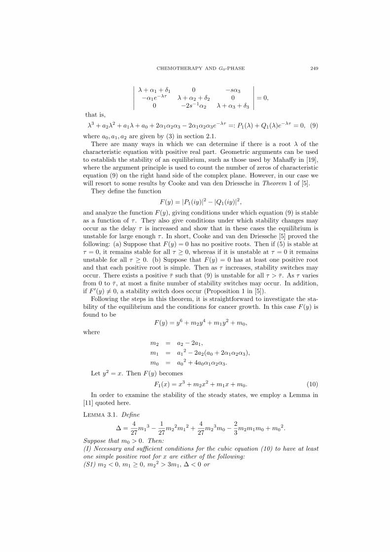
that is,

λ3 + a2λ2 + a1λ + a0 + 2α1α2α3 − 2α1α2α3e

−λτ =: P1(λ) + Q1(λ)e−λτ = 0, (9)

where a0, a1, a2 are given by (3) in section 2.1.There are many ways in which we can determine if there is a root λ of the

characteristic equation with positive real part. Geometric arguments can be usedto establish the stability of an equilibrium, such as those used by Mahaffy in [19],where the argument principle is used to count the number of zeros of characteristicequation (9) on the right hand side of the complex plane. However, in our case wewill resort to some results by Cooke and van den Driessche in Theorem 1 of [5].

They define the function

F (y) = |P1(iy)|2 − |Q1(iy)|2,and analyze the function F (y), giving conditions under which equation (9) is stableas a function of τ . They also give conditions under which stability changes mayoccur as the delay τ is increased and show that in these cases the equilibrium isunstable for large enough τ . In short, Cooke and van den Driessche [5] proved thefollowing: (a) Suppose that F (y) = 0 has no positive roots. Then if (5) is stable atτ = 0, it remains stable for all τ ≥ 0, whereas if it is unstable at τ = 0 it remainsunstable for all τ ≥ 0. (b) Suppose that F (y) = 0 has at least one positive rootand that each positive root is simple. Then as τ increases, stability switches mayoccur. There exists a positive τ such that (9) is unstable for all τ > τ . As τ variesfrom 0 to τ , at most a finite number of stability switches may occur. In addition,if F ′(y) 6= 0, a stability switch does occur (Proposition 1 in [5]).

Following the steps in this theorem, it is straightforward to investigate the sta-bility of the equilibrium and the conditions for cancer growth. In this case F (y) isfound to be

F (y) = y6 + m2y4 + m1y

2 + m0,

where

m2 = a2 − 2a1,

m1 = a12 − 2a2(a0 + 2α1α2α3),

m0 = a02 + 4a0α1α2α3.

Let y2 = x. Then F (y) becomes

F1(x) = x3 + m2x2 + m1x + m0. (10)

In order to examine the stability of the steady states, we employ a Lemma in[11] quoted here.

Lemma 3.1. Define

∆ =427

m13 − 1

27m2

2m12 +

427

m23m0 − 2

3m2m1m0 + m0

2.

Suppose that m0 > 0. Then:(I) Necessary and sufficient conditions for the cubic equation (10) to have at leastone simple positive root for x are either of the following:(S1) m2 < 0, m1 ≥ 0, m2

2 > 3m1, ∆ < 0 or


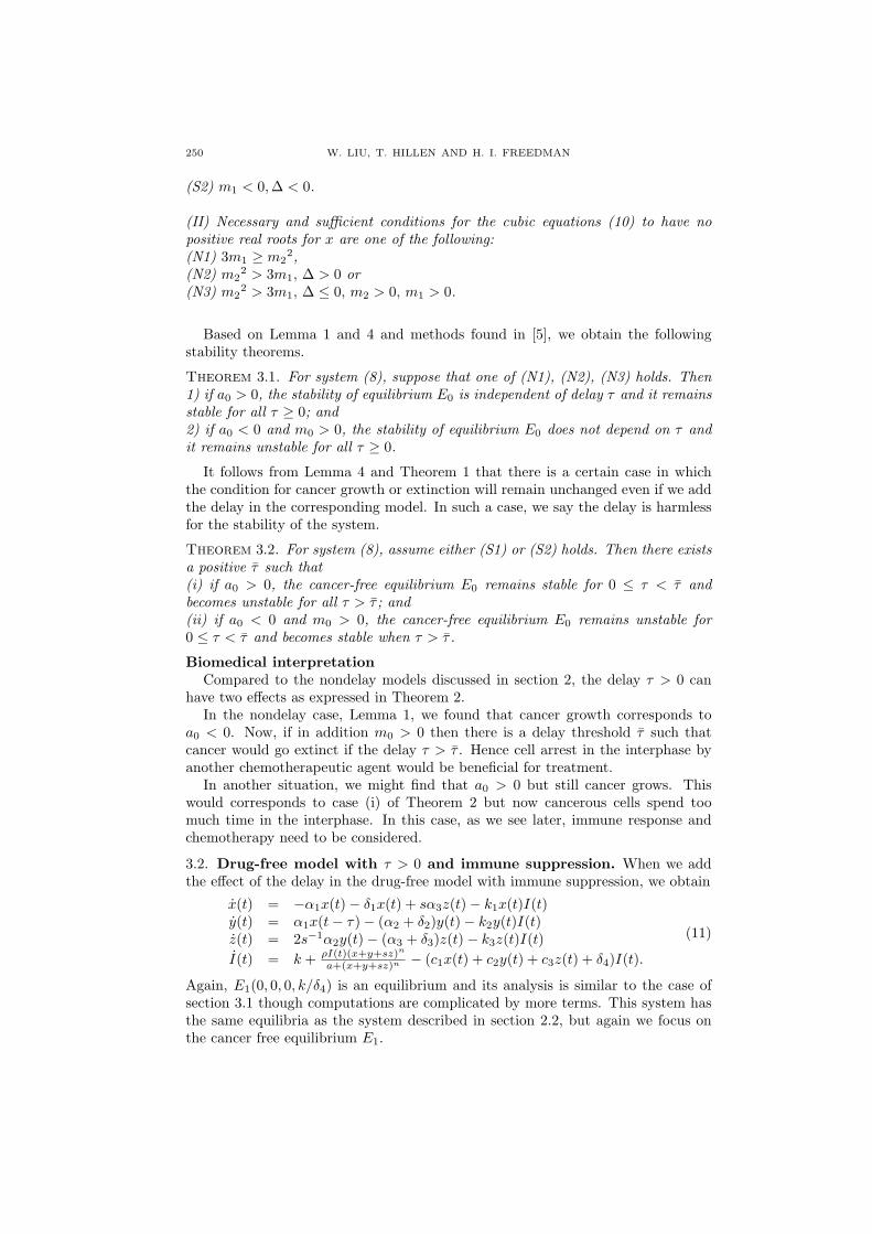
(S2) m1 < 0, ∆ < 0.

(II) Necessary and sufficient conditions for the cubic equations (10) to have nopositive real roots for x are one of the following:(N1) 3m1 ≥ m2

2,(N2) m2

2 > 3m1, ∆ > 0 or(N3) m2

2 > 3m1, ∆ ≤ 0, m2 > 0, m1 > 0.

Based on Lemma 1 and 4 and methods found in [5], we obtain the followingstability theorems.

Theorem 3.1. For system (8), suppose that one of (N1), (N2), (N3) holds. Then1) if a0 > 0, the stability of equilibrium E0 is independent of delay τ and it remainsstable for all τ ≥ 0; and2) if a0 < 0 and m0 > 0, the stability of equilibrium E0 does not depend on τ andit remains unstable for all τ ≥ 0.

It follows from Lemma 4 and Theorem 1 that there is a certain case in whichthe condition for cancer growth or extinction will remain unchanged even if we addthe delay in the corresponding model. In such a case, we say the delay is harmlessfor the stability of the system.

Theorem 3.2. For system (8), assume either (S1) or (S2) holds. Then there existsa positive τ such that(i) if a0 > 0, the cancer-free equilibrium E0 remains stable for 0 ≤ τ < τ andbecomes unstable for all τ > τ ; and(ii) if a0 < 0 and m0 > 0, the cancer-free equilibrium E0 remains unstable for0 ≤ τ < τ and becomes stable when τ > τ .

Biomedical interpretationCompared to the nondelay models discussed in section 2, the delay τ > 0 can

have two effects as expressed in Theorem 2.In the nondelay case, Lemma 1, we found that cancer growth corresponds to

a0 < 0. Now, if in addition m0 > 0 then there is a delay threshold τ such thatcancer would go extinct if the delay τ > τ . Hence cell arrest in the interphase byanother chemotherapeutic agent would be beneficial for treatment.

In another situation, we might find that a0 > 0 but still cancer grows. Thiswould corresponds to case (i) of Theorem 2 but now cancerous cells spend toomuch time in the interphase. In this case, as we see later, immune response andchemotherapy need to be considered.

3.2. Drug-free model with τ > 0 and immune suppression. When we addthe effect of the delay in the drug-free model with immune suppression, we obtain

x(t) = −α1x(t)− δ1x(t) + sα3z(t)− k1x(t)I(t)y(t) = α1x(t− τ)− (α2 + δ2)y(t)− k2y(t)I(t)z(t) = 2s−1α2y(t)− (α3 + δ3)z(t)− k3z(t)I(t)I(t) = k + ρI(t)(x+y+sz)n

a+(x+y+sz)n − (c1x(t) + c2y(t) + c3z(t) + δ4)I(t).

(11)

Again, E1(0, 0, 0, k/δ4) is an equilibrium and its analysis is similar to the case ofsection 3.1 though computations are complicated by more terms. This system hasthe same equilibria as the system described in section 2.2, but again we focus onthe cancer free equilibrium E1.


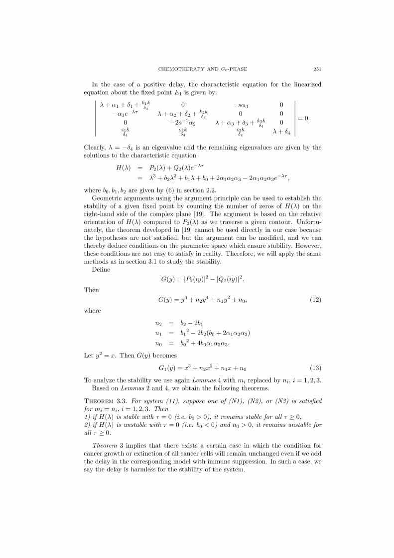
In the case of a positive delay, the characteristic equation for the linearizedequation about the fixed point E1 is given by:

∣∣∣∣∣∣∣∣∣

λ + α1 + δ1 + k1kδ4

0 −sα3 0−α1e

−λτ λ + α2 + δ2 + k2kδ4

0 00 −2s−1α2 λ + α3 + δ3 + k3k

δ40

c1kδ4

c2kδ4

c3kδ4

λ + δ4

∣∣∣∣∣∣∣∣∣= 0 .

Clearly, λ = −δ4 is an eigenvalue and the remaining eigenvalues are given by thesolutions to the characteristic equation

H(λ) = P2(λ) + Q2(λ)e−λτ

= λ3 + b2λ2 + b1λ + b0 + 2α1α2α3 − 2α1α2α3e

−λτ ,

where b0, b1, b2 are given by (6) in section 2.2.Geometric arguments using the argument principle can be used to establish the

stability of a given fixed point by counting the number of zeros of H(λ) on theright-hand side of the complex plane [19]. The argument is based on the relativeorientation of H(λ) compared to P2(λ) as we traverse a given contour. Unfortu-nately, the theorem developed in [19] cannot be used directly in our case becausethe hypotheses are not satisfied, but the argument can be modified, and we canthereby deduce conditions on the parameter space which ensure stability. However,these conditions are not easy to satisfy in reality. Therefore, we will apply the samemethods as in section 3.1 to study the stability.

DefineG(y) = |P2(iy)|2 − |Q2(iy)|2.

ThenG(y) = y6 + n2y

4 + n1y2 + n0, (12)

where

n2 = b2 − 2b1

n1 = b12 − 2b2(b0 + 2α1α2α3)

n0 = b02 + 4b0α1α2α3.

Let y2 = x. Then G(y) becomes

G1(y) = x3 + n2x2 + n1x + n0 (13)

To analyze the stability we use again Lemmas 4 with mi replaced by ni, i = 1, 2, 3.Based on Lemmas 2 and 4, we obtain the following theorems.

Theorem 3.3. For system (11), suppose one of (N1), (N2), or (N3) is satisfiedfor mi = ni, i = 1, 2, 3. Then1) if H(λ) is stable with τ = 0 (i.e. b0 > 0), it remains stable for all τ ≥ 0,2) if H(λ) is unstable with τ = 0 (i.e. b0 < 0) and n0 > 0, it remains unstable forall τ ≥ 0.

Theorem 3 implies that there exists a certain case in which the condition forcancer growth or extinction of all cancer cells will remain unchanged even if we addthe delay in the corresponding model with immune suppression. In such a case, wesay the delay is harmless for the stability of the system.


Theorem 3.4. For system (11), assume either (S1) or (S2) for mi = ni, i = 1, 2, 3holds. Then there exists a positive τ such that(i) if b0 > 0, the cancer-free equilibrium E1 remains stable for 0 ≤ τ < τ , andbecomes unstable for all τ > τ .(ii) if b0 < 0 and n0 > 0, the cancer-free equilibrium E1 remains unstable for0 ≤ τ < τ , and becomes stable for τ > τ .

Biomedical interpretationAs mentioned earlier, in the context of cancer models, stability switching as the

delay is varied is very important, because many cycle-specific drugs retain the cellsor trap them in a given phase, thus increasing the time a cell spends in a particularcompartment. For an example, if spindle assembly is blocked, then the point wherethe M state becomes unstable moves to a much higher mass/DNA value. As aconsequence, mitosis becomes a stable state, and cells entering into the M phasewill be stuck there [21].

This analysis shows that care must be taken when trapping the cells in a com-partment since the ultimate effect may be adverse: the cancer-free fixed point mayswitch from a stable equilibrium to an unstable one ( see (i) of Theorem 4). Thiswould mean that when the immune response is blocked, the system would not movetoward the disease-free state. On the other hand, it is possible to increase or de-crease the resident time during the interphase to “unlock” a fixed point from itsinstability and to push it toward the stable range (see (ii) of Theorem 4).

3.3. Drug model when τ > 0 with immune suppression. When we add theadministration of a delay, we obtain our full model (1). Again E2(0, 0, 0, k/δ4, 0) isan equilibrium and its analysis is similar to that shown in section 3.2. The systemhas the same equilibria as the system described in section 2.3, but again we focuson the cancer-free equilibrium E2.

In this case, the characteristic equation for the linearized equation about a fixedpoint E2 is given by

∣∣∣∣∣∣∣∣∣∣∣

λ + α1 + δ1 + k1kδ4

0 −sα3 0 0−α1e

−λτ λ + α2 + δ2 + k2kδ4

0 0 00 −2s−1α2 λ + α3 + δ3 + k3k

δ40 0

c1kδ4

c2kδ4

c3kδ4

λ + δ4−k6k7k

δ4

0 0 0 0 λ + γ

∣∣∣∣∣∣∣∣∣∣∣

= 0

Obviously, λ = −δ4, λ = −γ are two eigenvalues. The remaining eigenvalues aregiven as the solutions to the characteristic equation

F (λ) = λ3 + b2λ2 + b1λ + b0 + 2α1α2α3 − 2α1α2α3e

−λτ = 0,

where b2, b1, b0 are given by (6) in section 2.2 and the stability analysis of theequilibria is the same as for H(λ) in section 3.2. Thus we state the appropriatetheorems here.

Theorem 3.5. For system (14), suppose one of (N1), (N2), (N3) with mi = ni, i =1, 2, 3 holds. Then1) if b0 > 0, then E2 remains stable for all τ ≥ 0; and2) if b0 < 0 and n0 > 0, then E2 remains unstable for all τ ≥ 0.


Theorem 3.6. For system (14), assume either (S1) or (S2) with mi = ni, i = 1, 2, 3holds. Then there exists a positive τ such that(i) if b0 > 0, the cancer-free equilibrium E2 remains stable for 0 ≤ τ < τ , andbecomes unstable for all τ > τ ; and(ii) if b0 < 0 and n0 > 0, the cancer-free equilibrium E2 remains unstable for0 ≤ τ < τ , and becomes stable for τ > τ .

Biomedical interpretationThe interpretation of this result is the same as above. Under conditions (ii) a

cell arrest in the interphase is beneficial for treatment. For conditions (i) a longdelay in the interphase enables cells to avoid treatment and re-enter the M -phase.The next question, again, is the question of multiple treatments, which we will notstudy here; however, a numerical solution for multiple dosages is given in Figure 4.

3.4. Hopf bifurcation. With the aid of Theorem 1 in [5], it is also straightforwardto check for possible Hopf bifurcations for the full model (1), when we increasethe delay τ . The importance of Hopf bifurcations in this context is that at thebifurcation point a limit cycle is formed around the fixed point, resulting in stableperiodic solutions. The existence of periodic solutions is relevant in cancer modelsbecause it implies that the cancer levels may oscillate around a fixed point evenin the absence of any treatment. Such a phenomenon has been observed clinicallyand is known as “Jeff’s Phenomenon” [11]. Periodic oscillations also indicate cellsynchronization within the cell cycle. In this section, we will prove that such Hopfbifurcations can occur. Now consider a general characteristic equation for system(1):

λ3 + r2λ2 + r1λ + r0 − s0e

−λτ = 0. (14)Let λ = u + iv,(u, v ∈ R), and rewrite (14) in terms of its real and imaginary partsas

u3 − 3uv2 + r2(u2 − v2) + r1u + r0 = s0e−uτ cos(vτ)

3u2v − v3 + 2r2uv + r1v = −s0e−uτ sin(vτ). (15)

Let τ be such that u(τ) = 0. Then the above equations reduce to

−r2v2 + r0 = s0 cos(vτ)

−v3 + r1v = −s0 sin(vτ). (16)

It follows by taking the sum of squares that

v6 + (r22 − 2r1)v4 + (r1

2 − 2r2r0)v2 + r02 − s0

2 = 0. (17)

Suppose that v1 is the largest positive simple root of equation (17). Then with thisvalue of v1, (16) determines a τ1 uniquely such that u(τ1) = 0 and v(τ1) = v1. Toapply the Hopf bifurcation theorem as stated in Marsden & McCracken [20], westate and prove the following theorem.

Theorem 3.7. Suppose that equation (17) has at least one simple positive root andv1 is the largest such root. Then iv(τ1) = iv1 is a simple root of equation (14) andu(τ) + iv(τ) is differentiable with respect to τ in a neighborhood of τ = τ1.

Proof . To show that iv(τ1) = iv1 is a simple root, equation (14) can be writtenas f(λ) = 0 where

f(λ) = λ3 + r2λ2 + r1λ + r0 − s0e

−λτ . (18)

Any double root λ satisfies

f(λ) = 0, f ′(λ) = 0,


wheref ′(λ) = 3λ2 + 2r2λ + r1 + τs0e

−λτ . (19)Substituting λ = iv1 and τ = τ1 into (19) and equating real and imaginary parts ifiv1 is a double root, we obtain

−r2v21 + r0 = s0 cos(v1τ1)

−v31 + r1v1 = −s0 sin(v1τ1),

(20)

andr1 − 3v2

1 = −τ1s0 cos(v1τ)2r2v1 = τ1s0 sin(v1τ). (21)

Now, equation (16) can be written as F (v1) = 0, where

F (v) = (−r2v2 + r0)2 + (−v3 + r1v)2 − (s0)2 (22)

F ′(v) = 2(−r2v2 + r0)(−2r2v) + 2(−v3 + r1v)(−3v2 + r1). (23)

By substituting (20) and (21) into (22), (23), we obtain

F (v1) = F ′(v1) = 0.

Note that v1 is a double root of F (v1) = 0 and that F (v1) = F ′(v1) = 0, which isa contradiction as we have assumed that v1 is a simple root of (17). Hence iv1 is asimple root of equation (14), an analytic equation. By using the analytic version ofthe implicit function theorem (Chow & Hale [3]), we can see u(τ)+ iv(τ) is definedand analytic in a neighborhood of τ = τ1. ¤

Next, to establish Hopf bifurcation at τ = τ1, we need to verify the transversalitycondition

du

dτ|τ=τ1 6= 0.

By differentiating equations (16) with respect to τ and setting u = 0 and v = v1,we obtain

Adudτ |τ=τ1 + B dv

dτ |τ=τ1 = −s0v1 sin(v1τ1)−B du

dτ |τ=τ1 + A dvdτ |τ=τ1 = s0v1 cos(v1τ1),

(24)

where

A = r1 − 3v21 + s0τ1 cos(v1τ1)

B = −2r2v1 + s0τ1 sin(v1τ1).

Solving for dudτ , dv

dτ form (23) with the help of (16), we have

du

dτ|τ=τ1 =

v21 [3v4

1 + 2(r22 − 2r1)v2

1 + r12 − 2r2r0]

A2 + B2. (25)

Let z = v21 . Then equation (17) reduces to

Φ(z) = z3 + (r22 − 2r1)z2 + (r1

2 − 2r2r0)z + r02 − s0

2.

HencedΦdz

= 3z2 + 2(r22 − 2r1)z + r1

2 − 2r2r0.

Since v21 is the largest positive single root of equation (17), then

dΦdz|z=v2

1> 0.

Therefore,du

dτ|τ=τ1 =

v21

A2 + B2

dΦdz|z=v2

1> 0.


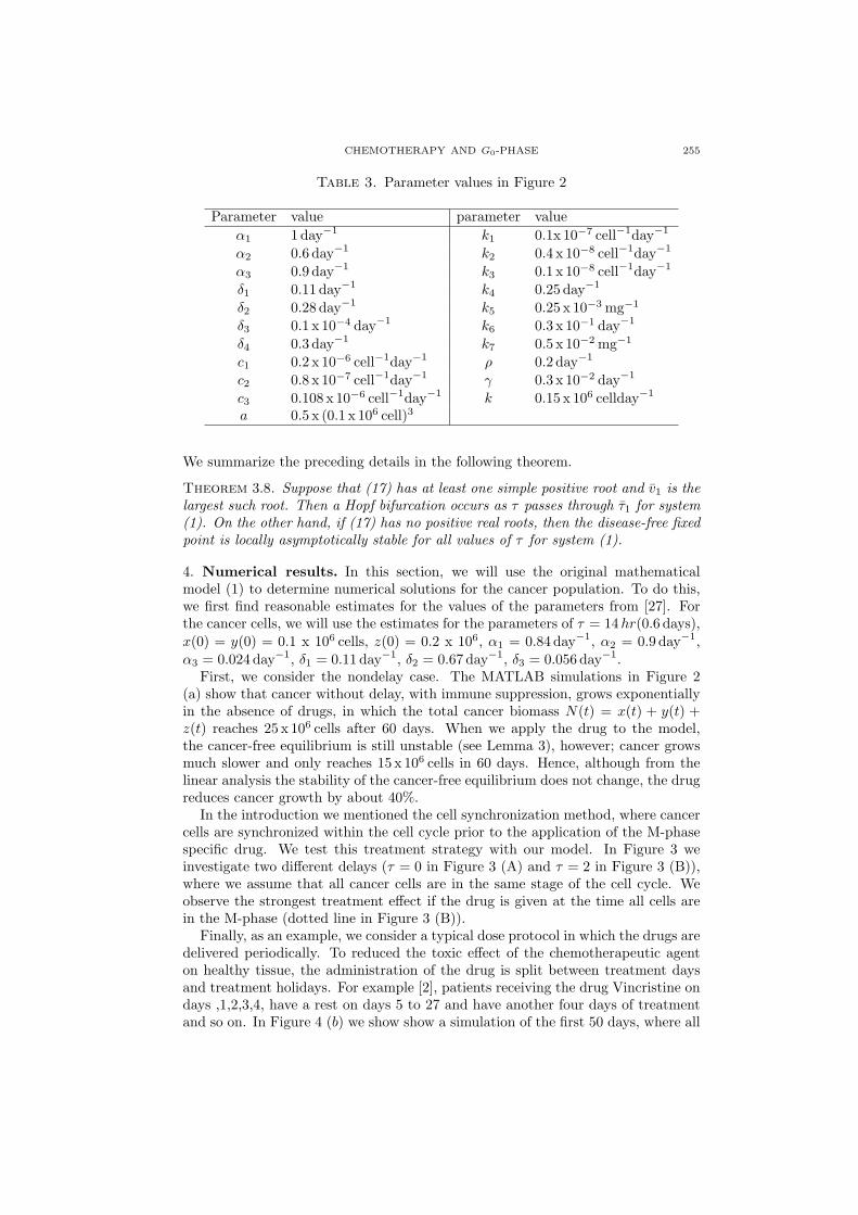
Table 3. Parameter values in Figure 2

Parameter value parameter valueα1 1 day−1 k1 0.1x 10−7 cell−1day−1

α2 0.6 day−1 k2 0.4 x 10−8 cell−1day−1

α3 0.9 day−1 k3 0.1 x 10−8 cell−1day−1

δ1 0.11 day−1 k4 0.25 day−1

δ2 0.28 day−1 k5 0.25 x 10−3 mg−1

δ3 0.1 x 10−4 day−1 k6 0.3 x 10−1 day−1

δ4 0.3 day−1 k7 0.5 x 10−2 mg−1

c1 0.2 x 10−6 cell−1day−1 ρ 0.2 day−1

c2 0.8 x 10−7 cell−1day−1 γ 0.3 x 10−2 day−1

c3 0.108 x 10−6 cell−1day−1 k 0.15 x 106 cellday−1

a 0.5 x (0.1 x 106 cell)3

We summarize the preceding details in the following theorem.

Theorem 3.8. Suppose that (17) has at least one simple positive root and v1 is thelargest such root. Then a Hopf bifurcation occurs as τ passes through τ1 for system(1). On the other hand, if (17) has no positive real roots, then the disease-free fixedpoint is locally asymptotically stable for all values of τ for system (1).

4. Numerical results. In this section, we will use the original mathematicalmodel (1) to determine numerical solutions for the cancer population. To do this,we first find reasonable estimates for the values of the parameters from [27]. Forthe cancer cells, we will use the estimates for the parameters of τ = 14 hr(0.6 days),x(0) = y(0) = 0.1 x 106 cells, z(0) = 0.2 x 106, α1 = 0.84 day−1, α2 = 0.9 day−1,α3 = 0.024 day−1, δ1 = 0.11 day−1, δ2 = 0.67 day−1, δ3 = 0.056 day−1.

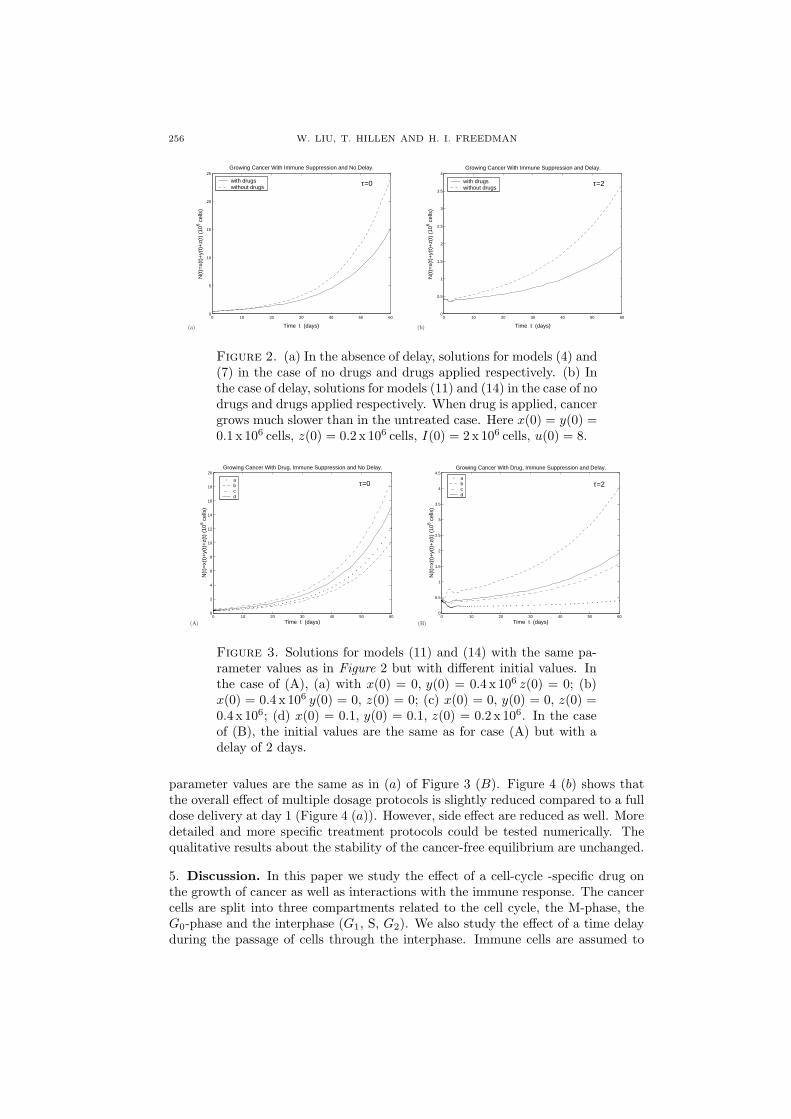
First, we consider the nondelay case. The MATLAB simulations in Figure 2(a) show that cancer without delay, with immune suppression, grows exponentiallyin the absence of drugs, in which the total cancer biomass N(t) = x(t) + y(t) +z(t) reaches 25 x 106 cells after 60 days. When we apply the drug to the model,the cancer-free equilibrium is still unstable (see Lemma 3), however; cancer growsmuch slower and only reaches 15 x 106 cells in 60 days. Hence, although from thelinear analysis the stability of the cancer-free equilibrium does not change, the drugreduces cancer growth by about 40%.

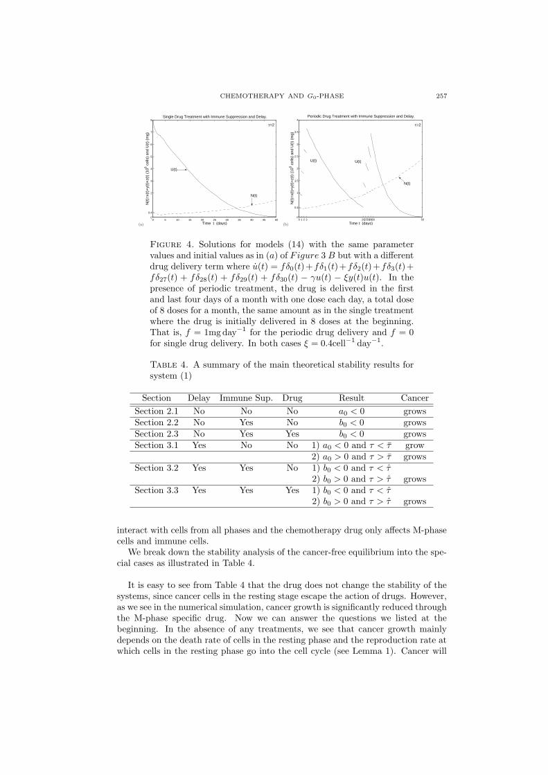
In the introduction we mentioned the cell synchronization method, where cancercells are synchronized within the cell cycle prior to the application of the M-phasespecific drug. We test this treatment strategy with our model. In Figure 3 weinvestigate two different delays (τ = 0 in Figure 3 (A) and τ = 2 in Figure 3 (B)),where we assume that all cancer cells are in the same stage of the cell cycle. Weobserve the strongest treatment effect if the drug is given at the time all cells arein the M-phase (dotted line in Figure 3 (B)).

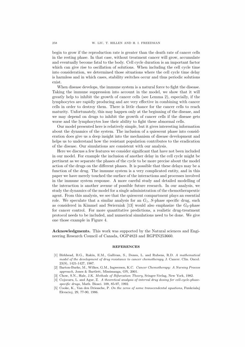
Finally, as an example, we consider a typical dose protocol in which the drugs aredelivered periodically. To reduced the toxic effect of the chemotherapeutic agenton healthy tissue, the administration of the drug is split between treatment daysand treatment holidays. For example [2], patients receiving the drug Vincristine ondays ,1,2,3,4, have a rest on days 5 to 27 and have another four days of treatmentand so on. In Figure 4 (b) we show show a simulation of the first 50 days, where all


(a)

0 10 20 30 40 50 600

5

10

15

20

25Growing Cancer With Immune Suppression and No Delay.

Time t (days)

N(t

)=x(

t)+

y(t)

+z(

t) (

106 c

ells

)

with drugswithout drugs τ=0

(b)

0 10 20 30 40 50 600

0.5

1

1.5

2

2.5

3

3.5

4Growing Cancer With Immune Suppression and Delay.

Time t (days)

N(t

)=x(

t)+

y(t)

+z(

t) (

106 c

ells

)

with drugswithout drugs

τ=2

Figure 2. (a) In the absence of delay, solutions for models (4) and(7) in the case of no drugs and drugs applied respectively. (b) Inthe case of delay, solutions for models (11) and (14) in the case of nodrugs and drugs applied respectively. When drug is applied, cancergrows much slower than in the untreated case. Here x(0) = y(0) =0.1 x 106 cells, z(0) = 0.2 x 106 cells, I(0) = 2 x 106 cells, u(0) = 8.

(A)

0 10 20 30 40 50 600

2

4

6

8

10

12

14

16

18

20Growing Cancer With Drug, Immune Suppression and No Delay.

Time t (days)

N(t

)=x(

t)+

y(t)

+z(

t) (

106 c

ells

)

abcd

τ=0

(B)

0 10 20 30 40 50 600

0.5

1

1.5

2

2.5

3

3.5

4

4.5Growing Cancer With Drug, Immune Suppression and Delay.

Time t (days)

N(t

)=x(

t)+

y(t)

+z(

t) (

106 c

ells

)

abcd

τ=2

Figure 3. Solutions for models (11) and (14) with the same pa-rameter values as in Figure 2 but with different initial values. Inthe case of (A), (a) with x(0) = 0, y(0) = 0.4 x 106 z(0) = 0; (b)x(0) = 0.4 x 106 y(0) = 0, z(0) = 0; (c) x(0) = 0, y(0) = 0, z(0) =0.4 x 106; (d) x(0) = 0.1, y(0) = 0.1, z(0) = 0.2 x 106. In the caseof (B), the initial values are the same as for case (A) but with adelay of 2 days.

parameter values are the same as in (a) of Figure 3 (B). Figure 4 (b) shows thatthe overall effect of multiple dosage protocols is slightly reduced compared to a fulldose delivery at day 1 (Figure 4 (a)). However, side effect are reduced as well. Moredetailed and more specific treatment protocols could be tested numerically. Thequalitative results about the stability of the cancer-free equilibrium are unchanged.

5. Discussion. In this paper we study the effect of a cell-cycle -specific drug onthe growth of cancer as well as interactions with the immune response. The cancercells are split into three compartments related to the cell cycle, the M-phase, theG0-phase and the interphase (G1, S, G2). We also study the effect of a time delayduring the passage of cells through the interphase. Immune cells are assumed to


(a)0 5 10 15 20 25 30 35 40 45 50

0

0.4

2

3

4

5

6

7

8Single Drug Treatment with Immune Suppression and Delay.

Time t (days)

N(t

)=x(

t)+

y(t)

+z(

t) (

106 c

ells

) an

d U

(t)

(mg)

U(t)

N(t)

τ=2

(b)

0 1 2 3 2627282930 500

0.4

1

1.5

2

2.5

3

3.5

4Periodic Drug Treatment with Immune Suppression and Delay.

Time t (days)

N(t

)=x(

t)+

y(t)

+z(

t) (

106 c

ells

) an

d U

(t)

(mg)

U(t) U(t)

N(t)

τ=2

Figure 4. Solutions for models (14) with the same parametervalues and initial values as in (a) of Figure 3 B but with a differentdrug delivery term where u(t) = fδ0(t)+fδ1(t)+fδ2(t)+fδ3(t)+fδ27(t) + fδ28(t) + fδ29(t) + fδ30(t) − γu(t) − ξy(t)u(t). In thepresence of periodic treatment, the drug is delivered in the firstand last four days of a month with one dose each day, a total doseof 8 doses for a month, the same amount as in the single treatmentwhere the drug is initially delivered in 8 doses at the beginning.That is, f = 1mg day−1 for the periodic drug delivery and f = 0for single drug delivery. In both cases ξ = 0.4cell−1 day−1.

Table 4. A summary of the main theoretical stability results forsystem (1)

Section Delay Immune Sup. Drug Result CancerSection 2.1 No No No a0 < 0 growsSection 2.2 No Yes No b0 < 0 growsSection 2.3 No Yes Yes b0 < 0 growsSection 3.1 Yes No No 1) a0 < 0 and τ < τ grow

2) a0 > 0 and τ > τ growsSection 3.2 Yes Yes No 1) b0 < 0 and τ < τ

2) b0 > 0 and τ > τ growsSection 3.3 Yes Yes Yes 1) b0 < 0 and τ < τ

2) b0 > 0 and τ > τ grows

interact with cells from all phases and the chemotherapy drug only affects M-phasecells and immune cells.

We break down the stability analysis of the cancer-free equilibrium into the spe-cial cases as illustrated in Table 4.

It is easy to see from Table 4 that the drug does not change the stability of thesystems, since cancer cells in the resting stage escape the action of drugs. However,as we see in the numerical simulation, cancer growth is significantly reduced throughthe M-phase specific drug. Now we can answer the questions we listed at thebeginning. In the absence of any treatments, we see that cancer growth mainlydepends on the death rate of cells in the resting phase and the reproduction rate atwhich cells in the resting phase go into the cell cycle (see Lemma 1). Cancer will


begin to grow if the reproduction rate is greater than the death rate of cancer cellsin the resting phase. In that case, without treatment cancer will grow, accumulateand eventually become fatal to the body. Cell cycle duration is an important factorwhich can give rise to oscillation of solutions. When including the cell cycle timeinto consideration, we determined those situations where the cell cycle time delayis harmless and in which cases, stability switches occur and thus periodic solutionsexist.

When disease develops, the immune system is a natural force to fight the disease.Taking the immune suppression into account in the model, we show that it willgreatly help to inhibit the growth of cancer cells (see Lemma 2), especially, if thelymphocytes are rapidly producing and are very effective in combining with cancercells in order to destroy them. There is little chance for the cancer cells to reachmaturity. Unfortunately, this may happen only at the beginning of the disease, andwe may depend on drugs to inhibit the growth of cancer cells if the disease getsworse and the lymphocytes lose their ability to fight these abnormal cells.

Our model presented here is relatively simple, but it gives interesting informationabout the dynamics of the system. The inclusion of a quiescent phase into consid-eration does give us a deep insight into the mechanism of disease development andhelps us to understand how the resistant population contributes to the eradicationof the disease. Our simulations are consistent with our analysis.

Here we discuss a few features we consider significant that have not been includedin our model. For example the inclusion of another delay in the cell cycle might bepertinent as we separate the phases of the cycle to be more precise about the modelaction of the drugs on the different phases. It is possible that these delays may be afunction of the drug. The immune system is a very complicated entity, and in thispaper we have merely touched the surface of the interactions and processes involvedin the immune system response. A more careful study and detailed modelling ofthe interaction is another avenue of possible future research. In our analysis, westudy the dynamics of the model for a single administration of the chemotherapeuticagent. From this analysis, we see that the quiescent compartment plays an essentialrole. We speculate that a similar analysis for an G1, S-phase specific drug, suchas considered in Kimmel and Swierniak [13] would also emphasize the G0-phasefor cancer control. For more quantitative predictions, a realistic drug-treatmentprotocol needs to be included, and numerical simulations need to be done. We giveone those example in Figure 4.

Acknowledgments. This work was supported by the Natural sciences and Engi-neering Research Council of Canada, OGP4823 and RGPIN253660.

REFERENCES

[1] Birkhead, B.G., Rakin, E.M., Gallivan, S., Dones, L. and Rubens, R.D. A mathematicalmodel of the development of drug resistance to cancer chemotherapy, J. Cancer. Clin. Oncol.23(9), 1421-1427, 1987.

[2] Barton-Burke, M., Wilkes, G.M., Ingwersen, K.C. Cancer Chemotherapy: A Nursing Processapproach, Jones & Bartlett, Mississauga, ON, 2001.

[3] Chow, S.N., Hale, J.K. Methods of Bifurcation Theory, Sringer-Verlag, New York, 1982.[4] Cojocaru, L. and Agur, Z. A theoretical analysis of interval drug dosing for cell-cycle-phase-

specific drugs, Math. Biosci. 109, 85-97, 1992.[5] Cooke, K., Van den Driessche, P. On the zeros of some transcendental equations, Funkcialaj

Ekvacioj, 29, 77-90, 1986.


[6] Coppel, W.A. Stability and Asympotic Behavior of Differential Equations, D.C. Heath,Boston, 1965.

[7] De Boer et al Macrophage T lymphocyte interactions in the anti-tumor immune response: Amathematical model, J. Immu. 134, 2748-2758, 1985.

[8] DeLisi, C and Resoigno, A. Immune surveillance and neoplasia: A minimal mathematicalmodel, B. Math. Biol., 39, 201-221, 1997.

[9] Eisen, M.M Mathematical Models in Cell Biology and Cancer Chemotherapy, Volume 30 ofLecture Notes in Biomathematics, Springer-Verlag, New York, 1979.

[10] Hillen, T. and Dawson, A. A cell cycle derivation of the linear quadratic model in radiationtreatment, in preparation, 2006.

[11] Khan, Q.J.A., Greenhalgh, D. Hopf bifurcation in epidemic models with a time delay invaccination, IAM J. Appl. Med. Biol. 16, 113-142, 1999.

[12] Kheifetz, Y., Kogan, Y., Agur, Z. Long-range predictability in models of cell populationssubjected to phase-specific drugs: Growth-rate approximation using properties of positivecompact operators, Mathematical Models & Methods in the Applied Sciences. In Press.

[13] Kimmel, M. and Swierniak, A. Using control theory to make cancer chemotherapy beneficalfrom phase dependence and resistant to drug resistance, J. Math. Biosci. , 2006.

[14] Kirschner, D., Panetta, J. Modeling immunotherapy of the tumor-immune interation, J.Math. Biol. 37, 235-252, 1998.

[15] Knolle, H. Cell Kinetic Modeling and the Chemotherapy of Cancer, Volume 75 of LectureNotes in Biomathematics, Springer-Verlag, New York, 1988.

[16] Kozusko, F. et al. A mathematical model of invitro cancer cell growth and treatment with theantimitoic agent curacin A, Math. Biosci. 170, 1-16, 2001.

[17] Kuznetsov, A., et al. Nonlinear dynamics of immunogenic tumors: Parameter estimationand global bifurcation analysis, B. Math. Biol., 56, 295-321, 1994.

[18] Mackey, M.C. Cell kinetic status of hematopoietic stem cells, Cell Prolif., 34, 71-83, 2001.[19] Mahaffy, J.: A test for stability of linear differential equations, Quart. Appl. Math. 40, 193-

202, 1982.[20] Marsden, J.E., McCracken, M. The Hopf Bifurcation and its Applications, Springer-Verlag,

New York, 1976.[21] Novak, B. and Tyson, J.J. Modelling the controls of the eukaryotic cell cycle, Biochem. Soc.

Trans. 31, 1526-1529, 2003.[22] Panetta, J. A mathematical model of periodically pulsed chemotherapy: Tumor metastasis in

a competitive environment, Bull. Math. Biol. 58, 425-447, 1996.[23] Prehn, R.T. Prospectives in oncogenesis: Does immunity stimulate or inhibit neoplasia?, J.

Reticuloendothel. Soc., 10, 1-18, 1971.[24] Rubinow, S.I. and Lebowitz, J.L.: A mathematical model of the acute myeloblastic leukemic

state in man, Biophys. Journal, 16, 897-910, 1976.[25] Swan, G.W. Tumor growth models and cancer chemotherapy, In Cancer Modeling , Volume

83, Chapter 3, (Edited by J.R. Thompson and B. Brown), Marcel Dekker, New York, 91-179,1987.

[26] Villasana, M., Ochoa, G. An optimal control problem for cancer cycle-phase-specificchemotherapy, to appear, IEEE TEC Journal, 2004.

[27] Villasana, M, Radunskaya, A. A delay differential equation model for tumor growth, J. Math.Biol. 47, 270-294, 2003.

[28] Webb, G.F. A cell population model of periodic chemotherapy treatment, InBiomedical Modeling and Simulation, Elsevier Science, 83-92, 1992.

Received on July 18, 2006. Accepted on September 25, 2006.

E-mail address: [email protected]



A MATHEMATICAL MODEL FOR -PHASE SPECIFIC -PHASE AND ...

Documents

Transcript of A MATHEMATICAL MODEL FOR -PHASE SPECIFIC -PHASE AND ...