A Markov Decision Model to Evaluate Outsourcing in Reverse Logistics

Marco A. Serrato

Department of Graduate and Continuing Education Programs.

Tecnológico de Monterrey, Campus Morelia.

Tel: 52-443-3226895

Fax: 52-443-3226800 x 3102

mserrato@itesm.mx

Morelia 58350. Mexico.

Sarah M. Ryan

Department of Industrial & Manufacturing Systems Engineering

Iowa State University

Tel: 515-294-4347

Fax: 515-294-3524

smryan@iastate.edu

Ames, Iowa 50011-2164 USA.

Juan Gaytan

Department of Industrial & Systems Engineering.

Tecnológico de Monterrey, Campus Toluca.

52-722-2799990

52-722-2799990 x 2222

jgaytan@itesm.mx

Toluca 50110. Mexico.

Abstract.

One of the most important decisions regarding reverse logistics (RL) is whether to

outsource such functions or not, due to the fact that RL does not represent a production or

distribution firm’s core activity. To explore the hypothesis that outsourcing RL functions is

more suitable when returns are more variable, we formulate and analyze a Markov decision

model of the outsourcing decision. The reward function includes capacity and operating

costs of either performing RL functions internally or outsourcing them, and the transitions

among states reflect both the sequence of decisions taken and a simple characterization of the

random pattern of returns over time. We identify nonrestrictive conditions on the cost

parameters and the return rate that guarantee the existence of an optimal threshold policy for

outsourcing. Under mild assumptions, this threshold is more likely to be crossed, the higher

the uncertainty in returns. A set of numerical examples illustrate how the threshold for

outsourcing decreases while the probability of crossing any fixed threshold increases with the

variability in the return volume. They also indicate that the threshold is more easily crossed

when the length of the product’s life cycle is shorter.

Keywords

Reverse Logistics, Outsourcing, Markov Decision Model, Monotone Policy, Product Life

Cycle.

1

Introduction.

Once a firm distributes its products to retailers and final consumers, its flow of

materials has not stopped: a substantial return flow of products may occur due to either

generous return policies or legislation that requires producers to accept responsibility for their

products at end-of-life. We consider reverse logistics (RL) to include all activities associated

with collecting, inspecting, reprocessing, redistributing, and disposing of items after they

were originally sold (see Figure 1). Although it has long been perceived as a nuisance, it has

recently been considered as an improvement area with the correct focus. Every

manufacturing, distribution or sales firm, irrespective of its size, types of products or

geographic location, can benefit from planning, implementing and controlling RL activities.

Unfortunately, not enough analytical models that assist in RL strategic decisions currently

exist.

Given that RL is not the firm’s core activity, one of the most important decisions to be

taken by any producer is whether or not to outsource such functions. Any organization might

decide whether to perform the RL functions internally, or to contract with a third-party

reverse logistics provider (3PRLP) to perform them. This decision is mostly identified as a

“take it or leave it” alternative, because the chosen strategy, once adopted, will not be

changed frequently. The management of returns is complicated by the substantial

uncertainties associated with their timing, volume and condition. This paper focuses on how

the uncertainty in returns affects the decision of whether or not to outsource their RL

management.

Our central hypothesis is that outsourcing RL is more suitable when returns are more

variable. This hypothesis arose from a qualitative analysis of the published literature on

outsourcing and RL, which is overviewed briefly in the next section. In Section 3, we

formulate and analyze a Markov decision model of the outsourcing decision. The reward

2

function includes the most significant components of the cost of either performing RL

functions internally or outsourcing them, and the transitions among states reflect both the

sequence of decisions taken and a simple characterization of the random pattern of returns

over time. We assume that RL functions initially are performed internally. In order to focus

simply on the outsourcing decision, we limit our attention to two possible actions in each

period: either adjust internal capacity to match the expected number of returns in the next

period, or switch permanently to outsourcing. By analyzing the cost and transition

probability functions, we identify nonrestrictive conditions for the existence of an optimal

monotone policy over the partially ordered state space, which reduces to a threshold of

cumulative returns, beyond which outsourcing is optimal. Such conditions are stated in terms

of the cost parameters involved, as well as the return rate for the product considered. Finally,

we show that under mild assumptions, this threshold is more likely to be crossed when the

uncertainty in returns is higher. Numerical examples that illustrate how the threshold for

outsourcing decreases while the probability of crossing any fixed threshold increases with the

variability in the return volume lend further support to the hypothesis. These numerical

examples demonstrate not only how the threshold is easily crossed when the variability on the

return volume increases, but also when the length of the product’s life cycle is shorter.

Finally, in Section 4, we draw conclusions and outline future research that can be

developed based on this work.

2. Literature Review on Outsourcing RL Functions

There are many reasons why products are returned, either by consumers or by the companies

involved in the distribution chain. Retailers may return products because of damage in transit,

expired date code, the model being discontinued or replaced, seasonality, excessive retailer

inventories, retailer going out of business, etc. On the other hand, consumers can return

3

products for such reasons as quality problems, failure to meet the consumer’s needs, for

remanufacturing, or for proper disposal.

Also, once products have reached the end of their useful life, they may be able to be

remanufactured, refurbished or repaired; thus extending their life. These options can provide

significant benefits in some instances, especially for products that have modular components

(e.g. electronic equipment, computers) that can be replaced, upgraded and/or refurbished. The

value of items that are remanufactured typically will be lower than that of the same items

produced for the first time. However, their value will be substantially higher than that of

items being sold for scrap, salvage or recycling (Stock, 1998).

The importance of RL has increased in recent years. Currently, estimates of annual

sales of remanufactured products exceed $50 billion in the United States alone (Guide and

van Wassenhove, 2003). There are no worldwide estimates of the economic scope of reuse

activities, but the number of firms engaged in this sector is growing rapidly in response to the

opportunities to create additional wealth, and in response to the enactment of extended

producer responsibility legislation in several countries. Unfortunately, even with this

significant development of the RL market in recent years, not enough analytical models that

assist in RL strategic decisions currently exist. In a survey of current literature, Dowlatshahi

(2005) identified the present state of theory in RL.

A number of researchers have addressed problems and opportunities in RL

management. Guide and van Wassenhove (2003) argued that closed-loop supply chains

(which are composed of the typical forward-supply network and the RL network) can be

viewed as a business proposition where profit maximization is the objective. The

characteristics of such maximization will depend on the forward supply chain characteristics,

as well as the RL network composition. Some recent research considers both forward and

reverse activities simultaneously, e.g., Vaidyanathan (2006) adopted an analytical approach

4

to address production planning in closed-loop supply chains, with product recovery and

reuse. However, the management of RL activities is complicated by factors that are less

prevalent in the forward supply chain.

Uncertainty in product returns complicates several aspects of RL management. For

example, recent work by Nakashima et al. (2004) illustrated how this uncertainty, which they

characterized in terms of a virtual inventory level, can be modeled in a Markov decision

process for controlling a remanufacturing system.

The product life cycle is another critical factor regarding RL systems. Tibben-Lembke

(2002) clearly explained its importance in the analysis of RL systems. In this vein, Bufardi et

al. (2004) developed a multicriteria decision-aid approach for product end-of-life alternative

selection. Also, Gonzalez et al. (2005) developed a new approach for enhancing reuse

alternatives to reduce environmental problems from the earliest stages of product life cycle.

Frequently, uncertainty in returns combines with a short product life cycle to increase

the complexity of decisions that may have significant economic impact. Tang et al. (2004)

performed a detailed economic evaluation of disassembly processes for remanufacturing

systems. Also, Willems et al. (2006) developed a linear programming approach to

quantifying the turning point to make disassembly economically viable. The cost of

managing a returned item is one of the most important factors when choosing how to dispose

of it, as well as the price to be received for it, if such a price exists. The factors to consider

will differ according to the characteristics of the RL system, such as its size, characteristics,

products manufactured, managerial strategies and goals, etc. The amount of money invested

in these activities will be a critical issue too.

Outsourcing to a 3PRLP has been identified as one of the most important management

strategies for RL networks in the recent years. Razzaque and Sheng (1998) surveyed the

literature related to outsourcing logistics functions. With regard to RL functions, Meade and

5

Sarkis (2002) stated three different choices that can be made: to do nothing, to develop an

internal RL function, or to find a 3PRLP and partner with them. They developed a model for

selecting and evaluating 3PRLP. However, this model does not represent a tool for

determining whether or not to outsource RL activities, but rather it helps in the decision of

selecting a 3PRLP once the firm has chosen the outsourcing strategy. Krumwiede and Sheu

(2002) showed a particular model for market entry by a 3PRLP, which helps those companies

who would like to pursue RL as a new market. However, Dowlatshahi (2000) warned that

some such firms are not really prepared to effectively address these service needs due to the

lack of knowledge of RL networks.

One of the most important issues is to define whether the firm considers RL activities

as part of its core functions. When this is not the case, outsourcing might represent a good

alternative in order to allow the firm to focus on its core activities (Wu, et al., 2005).

In a detailed qualitative analysis, Serrato (2006) found that some of the most

important 3PRLPs are located in industry sectors with high return variability, as well as a

short length for the product life cycle. Due to the extremely high variability in the rate of

returns for the products managed in these RL systems, it is not economically feasible for a

firm to maintain its own RL facilities to deal with that flow, given that the amount of units to

be returned will be significantly uncertain over time, and the required capacity will be

changing constantly. The complexity of this situation increases when the life cycle for this

type of products is extremely short, which requires quick but adequate decisions for these RL

systems, in order to efficiently respond to such changing conditions. This response can be

accomplished effectively by involving a 3PRLP, which specializes in these activities, and can

take advantage of the economies of scale to convert RL functions into a profit-creating

activity in the closed-loop chain.

6

On the other hand, not many 3PRLPs are active in industry sectors with lower return

variability and longer product life cycles, because it is easier for the producer to develop its

own facilities to deal with the return flow, even though RL may not be part of its core

activities. The relatively low uncertainty in the amount of returns, and the longer time periods

for planning, developing and implementing RL systems, allow these firms to implement their

own RL systems without a particular need for another party involved. Serrato (2006)

developed a detailed analysis of these conclusions regarding outsourcing RL functions.

3. Markov Decision Model.

The MDM is designed to include the major cost drivers in the outsourcing decision, the

uncertainty in the return volume, temporal variability in sales, and the impracticality of

multiple transitions between performing RL functions internally and outsourcing them. To

simplify the focus on return volume variability, we assume that sales can be estimated

accurately from historical data related to this scenario and therefore are known. Returns

depend on the amount of units previously sold and the fraction of them that will be returned

through the firm’s RL system. Define the following notation:

L = Length of the product life cycle, which will depends on the particular RL scenario

considered.

W = Time length defined by the firm to continue managing the returns for the product

analyzed, after the last sale was made.

T = Length of the horizon analysis, T=L+W.

t = Decision epoch, t = 1, …, T – 1, where decision epoch t represents the end of period t.

Time T corresponds to the end of the problem horizon, where no decision is taken.

st = Amount of units sold by the firm during period t.

7

St = Cumulative sales experienced by the firm from period 1 through the end of period t,

1

tt ii

S s=

= ∑ .

r = Return rate, i.e., the expected fraction of units previously sold but not yet returned that

will be returned in the next period.

xt = Amount of units returned in period t.

wt =Cumulative amount of units returned from period 1 to the end of period t, 1

tt ii

w x=

=∑ .

kt = RL capacity held by the firm at the beginning of period t, which represents the number of

units that can be processed in a single period.

nt= Number of units outstanding in the market at the end of period t, ttt wSn −= .

The following assumptions underlie the MDM:

Assumption 1: The sales in each period of the study horizon are known.

Assumption 2: Each item that has been sold but not returned has a fixed probability,

r, of being returned in the next period, independent of all other items. This is consistent with

Toktay et al. (2003), where the number of periods between when a product was sold and

when it was returned was modeled as a geometrically distributed random variable. It follows

that knowing nt at time t, the number of returns in period t+1 has a binomial distribution with

parameters nt and r, such that the expected amount of returns in the next period can be

obtained as:

( ) rnxE tt =+1 , (1)

and the variability in the number of returns is:

( ) ( )rrnxVar tt −=+ 11 . (2)

Note that the variability increases as nt increases, for fixed r. Then, the variability in the

return volume increases as the number of outstanding units increases. The variability also

8

increases as r approaches 0.5 from below. However, as Rogers and Tibben-Lembke (1999)

observe, the return rate in most industries is between zero and 0.3, approaching 0.5 only in

some specific industry sectors.

Assumption 3: The firm’s RL capacity is continuous; i.e., it can be added or

subtracted in any quantity. This implies that the policy followed by any firm when adjusting

its RL capacity can consider any number of capacity units. However, to simplify the model

and focus on the structure of an optimal policy, we assume that if reverse logistics functions

are carried out internally, then the capacity will be adjusted to equal the expected number of

returns in the next period.

Assumption 4: If the number of returns in a period exceeds the RL capacity, the firm

pays a shortage penalty, which represents the cost of either disposal or outsourcing the return

processing on a temporary, emergency basis. No returns are carried over to a future period to

be processed later. This assumption is relevant when returns are economically perishable, so

that the positive value to be gained from handling them promptly is lost or greatly diminished

by delay; or when storage is not physically feasible.

Additional assumptions concerning costs are given later in this section.

3.1. Model Definition.

3.1.1. States.

The system state at each decision epoch t is defined as:

( ), for 1,2, ...,t tk w t T=

where kt represents the RL capacity owned by the firm during period t, measured in units per

period and wt is the cumulative number of returns through the end of period t. As described

below, the system states are partially ordered according to wt. At decision epoch 0, the system

9

state is ( )0, 00 =wk ; i.e., given an initial RL capacity 0k , no returns are yet experienced by the

firm.

3.1.2. Actions.

Given that the purpose of the MDM is to determine whether and when to outsource, it is

assumed that at the end of any period t, either of the following actions can be taken:

a = 0: Continue performing the RL activities internally by updating the firm’s

capacity to the expected amount of returns in the next period:

( ) rnxEk ttt == ++ 11 (3)

a=1: Adopt an outsourcing strategy for the RL activities by having a 3PRLP perform

such activities and taking the firm’s RL capacity to zero; i.e., kt+1 = 0. Given

that RL does not represent a core activity for the firm, it is also assumed that

once the outsourcing decision is taken, it remains in place for the rest of the

problem horizon.

Given that tn is an integer and that the capacity levels 1+tk are adjusted according to equation

(3) over a finite horizon, the problem has a discrete state space.

3.1.3. Transition Probabilities.

As the returns in each period follow a binomial distribution derived from the system state,

and given that the sales function is also known, the transition probability values between

states are defined as:

( ) ( ) { }1 1 1, , , for 0, 1t t t t tp k w k w a a+ + +⎡ ⎤ ∈⎣ ⎦ , (4)

where for a = 0 we have:

( ) ( ) ( )1

1 for 0,1,...,, , ,0

0 otherwise

tn jt jt

t t t t t

nr r j n

p n r w j k w j−

+

⎧⎛ ⎞− =⎪⎜ ⎟⎡ ⎤+ = ⎨⎝ ⎠⎣ ⎦

⎪⎩

(5)

10

and for a = 1 we have:

( ) ( ) ( )1

1 for 0,1,...,0, , ,1

0 otherwise.

tn jt jt

t t t t

nr r j n

p w j k w j−

+

⎧⎛ ⎞− =⎪⎜ ⎟⎡ ⎤+ = ⎨⎝ ⎠⎣ ⎦

⎪⎩

(6)

That is, the action taken determines the next period’s capacity, but the second state variable

1tw + depends only on ttt wSn −= according to the binomial distribution for the returns.

3.1.5. Rewards.

Define the following set of costs, where a capacity unit represents firm’s ability to process

one returned item during a single period:

c1: Unit investment cost for increasing the firm’s capacity ($/capacity unit).

c2: Unit capacity disinvestment cost ($/capacity unit).

c3: Fixed internal cost ($/capacity unit/period).

c4: Unit internal labor cost ($/unit).

c5: Unit shortage cost ($/unit).

c6: Unit capacity salvage value ($/capacity unit).

c7: Unit outsourcing cost ($/unit).

We assume c1, c3, c4, c5, c7 > 0 because they represent costs for the firm, while c2 and c6 are

unrestricted in sign, which allows the net cost of contracting capacity and salvaging

equipment to be positive or negative. Figure 1 shows where these costs are located in the RL

chain.

Figure 1. Relationship between RL chain and costs considered in the MDM.

Given that RL does not represent a core activity for the firm, profits from remanufacturing

are not considered. The next relationships are assumed between these cost parameters:

11

)11()10(

)9()8()7(

4315

57

74

23

21

cccccccccccc

++≥<<≥

≥

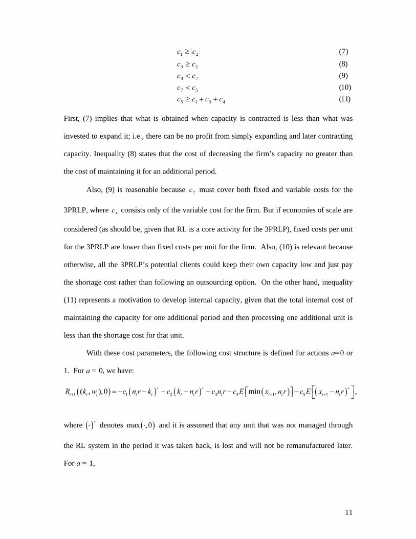
First, (7) implies that what is obtained when capacity is contracted is less than what was

invested to expand it; i.e., there can be no profit from simply expanding and later contracting

capacity. Inequality (8) states that the cost of decreasing the firm’s capacity no greater than

the cost of maintaining it for an additional period.

Also, (9) is reasonable because 7c must cover both fixed and variable costs for the

3PRLP, where 4c consists only of the variable cost for the firm. But if economies of scale are

considered (as should be, given that RL is a core activity for the 3PRLP), fixed costs per unit

for the 3PRLP are lower than fixed costs per unit for the firm. Also, (10) is relevant because

otherwise, all the 3PRLP’s potential clients could keep their own capacity low and just pay

the shortage cost rather than following an outsourcing option. On the other hand, inequality

(11) represents a motivation to develop internal capacity, given that the total internal cost of

maintaining the capacity for one additional period and then processing one additional unit is

less than the shortage cost for that unit.

With these cost parameters, the following cost structure is defined for actions a=0 or

1. For a = 0, we have:

( ) ( ) ( ) ( ) ( )1 1 2 3 4 1 5 1( , ),0 min , ,t t t t t t t t t t t tR k w c n r k c k n r c n r c E x n r c E x n r+ + ++ + +

⎡ ⎤= − − − − − − − −⎡ ⎤⎣ ⎦ ⎣ ⎦

where ( )+⋅ denotes ( )max ,0⋅ and it is assumed that any unit that was not managed through

the RL system in the period it was taken back, is lost and will not be remanufactured later.

For a = 1,

12

( )1 6 71 1

( , ),1 , where 0 1T T

t t t t t l ll t l t

R k w c k c n s s if t L+= + = +

⎛ ⎞= − + = + >⎜ ⎟

⎝ ⎠∑ ∑

Here, 7c corresponds to the payment made to the 3PRLP for the expected returns from

period t+1 onwards. Recall that, given that RL is not a core activity, it is assumed that when

taken, the outsourcing option will remain in effect for the remainder of the planning horizon.

Recall also from assumption 1, that the future sales can also be estimated accurately. This

function also implies that the 3PRLP has infinite capacity, given the fact that RL does

represent a core activity for it.

Also, we have the terminal reward in period T:

( ) { }6 5, , , for 0,1 and 0T T T T T TR k w a c k c n a k= − ∈ >

because the RL capacity defined by the firm is taken to zero in the last period, incurring the

corresponding salvage value. Also, this function reflects the cost incurred by not being able to

remanufacture any expected returned unit during period T or later.

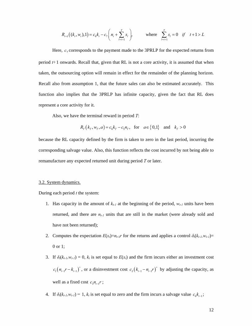
3.2. System dynamics.

During each period t the system:

1. Has capacity in the amount of kt-1 at the beginning of the period, wt-1 units have been

returned, and there are nt-1 units that are still in the market (were already sold and

have not been returned);

2. Computes the expectation E(xt)=nt-1r for the returns and applies a control δt(kt-1,wt-1)=

0 or 1;

3. If δt(kt-1,wt-1) = 0, kt is set equal to E(xt) and the firm incurs either an investment cost

( )1 1 1t tc n r k +− −− , or a disinvestment cost ( )2 1 1t tc k n r +

− −− by adjusting the capacity, as

well as a fixed cost 3 1tc n r− ;

4. If δt(kt-1,wt-1) = 1, kt is set equal to zero and the firm incurs a salvage value 6 1tc k − ;

13

5. Experiences a random amount of returns xt, which determines the new system state

( )tttt xwwk += −1, , as well as an amount of sales st, which determines the new

cumulative sales level for the firm (St = St-1 + st).

6. Incurs either an internal or a shortage cost, ( )4 1min ,t tc x n r− ) or ( )5 1t tc x n r +−− ,

respectively, if δt(kt-1,wt-1) = 1 and outsourcing cost 7 1

T

t ll t

c n s−=

⎛ ⎞+⎜ ⎟

⎝ ⎠∑ , otherwise.

Given an initial system state (k0,w0)= 0, the problem is to find a sequence of decision

functions {δ1*(k0,w0), δ2

*(k1,w1), …, δT*(kT-1,wT-1)} that maximizes the total expected reward.

The optimal policy is obtained by solving recursively:

where ( )ttt wku , represents the maximum expected reward earned by continuing optimally

from state ( )tt wk , onwards. This reward is obtained when taking action ( )ttt wka ,* , which

represents the optimal action a to take when in state ( )tt wk , .

3.3. Characteristics of the optimal policy to be found.

In principle, the recursive equation can be solved backwards from period T to identify the

optimal action for each possible state. However, depending on the length of the study

horizon, the sales volumes, and the granularity of the state space (i.e., the definition of a

“unit” sold or processed), the number of states to be evaluated could grow very large. To

reduce the amount of computation as well as improving communication, appeal to decision-

makers, and managerial insight, it is desirable to identify that an optimal policy of a simple

form exists. In particular, based on a partial ordering of the state space, below we establish

the existence of an optimal monotone policy, which corresponds to a threshold in one of the

( )( ) ( ) ( )( ) ( )

( )

1 1 10

1

( , ),0 , , ,0 , ,, max

( , ),1

tn

t t t t t t t t t t tjt t t

t t t

R k w p n r w j k w u n r w ju k w

R k w

+ + +=

+

⎧ ⎫+ + +⎪ ⎪= ⎨ ⎬

⎪ ⎪⎩ ⎭

∑

14

state variables, beyond which the outsourcing action a = 1 is optimal. Such a form also

facilitates exploration of conditions under which outsourcing is more likely to be optimal.

Below this threshold, the firm should continue performing the RL activities internally (a =

0). Next, conditions for the existence of an optimal deterministic nondecreasing policy will

be defined in terms of the MDM proposed.

3.3.1. Conditions for identifying a monotone deterministic nondecreasing policy as optimal.

As stated by Puterman (1994), there exist sets of conditions that ensure that optimal policies

are monotone in the system state. For such a concept to be meaningful, it is required that the

state have a physical interpretation and some natural ordering. The expression “monotone

policy” refers to a monotone deterministic Markovian policy.

For the MDM proposed, the states are partially ordered in terms of the cumulative

returned units wt. Specifically, for each t, let the states (kt, wt) be strictly partially ordered

according to the next criteria:

1. For every t, group the states where kt has a particular value (defined as ftk , g

tk , htk …).

2. For each group generated, generate a logical ordering for the states according to wt,

i.e; the larger wt is, the greater the state is.

This strict partial ordering implies that ( ) ( ) 21212211 ,, wwandkkwkwk <=⇔≺ , which is

illustrated in Figure 2.

Figure 2. Criterion followed for a strict partial state ordering.

In addition to the partial ordering defined, a cumulative probability also has to be defined in

order to identify the conditions for a monotone nondecreasing policy:

15

( ) ( ) ( ) ( )1

1 1 1, , , , , ,t

t l

n

t t l t t t t t t tw w

q k w k w a p k w k w a−

− − −=

⎡ ⎤ ⎡ ⎤=⎣ ⎦ ⎣ ⎦∑ ,

where for a = 0 we have:

( ) ( ) ( )1

1

1

11

1 1 1

1

1, , ,0

1

tt

l t

nn jt j

l tj w wt t l t t

l t

nr r for w w

q n r w k w jfor w w

−−

−

−−−

= −− − −

−

⎧ ⎛ ⎞− ≥⎪ ⎜ ⎟⎡ ⎤ = ⎨ ⎝ ⎠⎣ ⎦

⎪ <⎩

∑

and for a = 1 we have:

( ) ( ) ( )1

1

1

11

1 1

1

10, , ,1

1

tt

l t

nn jt j

l tj w wt l t t

l t

nr r for w w

q w k w jfor w w

−−

−

−−−

= −− −

−

⎧ ⎛ ⎞− ≥⎪ ⎜ ⎟⎡ ⎤ = ⎨ ⎝ ⎠⎣ ⎦

⎪ <⎩

∑

Finally, recall the definition of a superadditive function. Let X and Y be partially

ordered sets and g(x,y) a real-valued function on X ×Y. It is said that g is superadditive if for

x x− +≤ in X and y y− +≤ in Y,

( ) ( ) ( ) ( )+−−+−−++ +≥+ yxgyxgyxgyxg ,,,, .

One set of conditions stated by Puterman (1994) for the existence of a monotone optimal

policy are:

1. Rt((k,w),a) is nondecreasing in (k,w) for { }0,1a∈ ,

2. qt[(kt,wt=wl)⏐(k,w),a] is nondecreasing in (k,w) for all wl and { }0,1a∈ ,

3. Rt((k,w),a) is a superadditive function on (k,w) × a,

4. qt[kt,wt=wl)⏐(k,w),a] is a superadditive function on (k,w) × a, and

5. RT(kT,wT) is nondecreasing in (kT,wT).

When all of these conditions are satisfied, there exists a monotone nondecreasing policy that

is optimal.

3.4. Requirements in the MDM for the existence of a Monotone Nondecreasing Policy

16

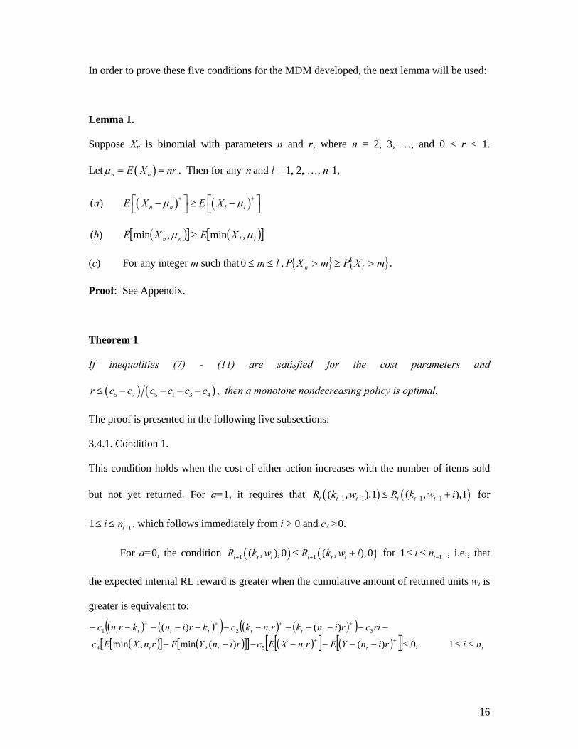
In order to prove these five conditions for the MDM developed, the next lemma will be used:

Lemma 1.

Suppose Xn is binomial with parameters n and r, where n = 2, 3, …, and 0 < r < 1.

Let ( )n nE X nrμ = = . Then for any n and l = 1, 2, …, n-1,

( ) ( )( ) n n l la E X E Xμ μ+ +⎡ ⎤ ⎡ ⎤− ≥ −⎣ ⎦ ⎣ ⎦

( )[ ] ( )[ ]llnn XEXEb μμ ,min,min)( ≥

(c) For any integer m such that lm ≤≤0 , { } { }mXPmXP ln >≥> .

Proof: See Appendix.

Theorem 1

If inequalities (7) - (11) are satisfied for the cost parameters and

( ) ( )5 7 5 1 3 4r c c c c c c≤ − − − − , then a monotone nondecreasing policy is optimal.

The proof is presented in the following five subsections:

3.4.1. Condition 1.

This condition holds when the cost of either action increases with the number of items sold

but not yet returned. For a=1, it requires that ( ) ( )1 1 1 1( , ),1 ( , ),1t t t t t tR k w R k w i− − − −≤ + for

11 ti n −≤ ≤ , which follows immediately from i > 0 and c7 >0.

For a=0, the condition ( ) ( )1 1( , ),0 ( , ),0t t t t t tR k w R k w i+ +≤ + for 11 ti n −≤ ≤ , i.e., that

the expected internal RL reward is greater when the cumulative amount of returned units wt is

greater is equivalent to:

( ) ( )( ) ( ) ( )( )( )[ ] ( )[ ][ ] ( )[ ] ( )[ ][ ] ttttt

tttttttt

nirinYErnXEcrinYErnXEc

ricrinkrnkckrinkrnc

≤≤≤−−−−−−−

−−−−−−−−−−−−++

++++

1,0)()(,min,min

)()(

54

321

17

where c1, c3, c4, c5>0 and X (Y) is binomially distributed with parameters nt (nt – i),

respectively, and r. From parts (a) and (b) of Lemma 1, the elements that multiply c4 and c5

are nonnegative.

This inequality can be analyzed in three cases:

( )( )

1)2)

3)

t t

t t

t t t

n r kk n i r

n i r k n r

<

≤ −

− ≤ ≤

In the first case, it is equivalent to:

( ) ( ) ( )

( ) ( )

3 2 4

5

min , min , ( )

( ) 0, 1

t t

t t t

ir c c c E X n r E Y n i r

c E X n r E Y n i r i n+ +

⎡ ⎤− − − − −⎡ ⎤ ⎡ ⎤⎣ ⎦ ⎣ ⎦⎣ ⎦⎡ ⎤⎡ ⎤ ⎡ ⎤− − − − − ≤ ≤ ≤⎣ ⎦ ⎣ ⎦⎣ ⎦

which is satisfied, given inequality (12). In the second case, it can be reduced to:

( ) ( ) ( )

( ) ( )1 3 4

5

min , min , ( )

( ) 0, 1

t t

t t t

ir c c c E X n r E Y n i r

c E X n r E Y n i r i n+ +

⎡ ⎤− + − − −⎡ ⎤ ⎡ ⎤⎣ ⎦ ⎣ ⎦⎣ ⎦⎡ ⎤⎡ ⎤ ⎡ ⎤− − − − − ≤ ≤ ≤⎣ ⎦ ⎣ ⎦⎣ ⎦

which follows from the assumption of positive cost coefficients. Finally, for the last case it

is:

( )( ) ( ) ( )

( ) ( )

1 2 4

5

min , min , ( )

( ) 0, 1

t t t t

t t t

k n r c c c E X n r E Y n i r

c E X n r E Y n i r i n+ +

⎡ ⎤− + − − −⎡ ⎤ ⎡ ⎤⎣ ⎦ ⎣ ⎦⎣ ⎦⎡ ⎤⎡ ⎤ ⎡ ⎤− − − − − ≤ ≤ ≤⎣ ⎦ ⎣ ⎦⎣ ⎦

which holds under inequalities (7) and (8).

3.4.2. Condition 2.

This condition holds when it is more likely to meet or exceed a given number of cumulative

returns in the next period, if a higher number of returns have been experienced up to the

current period. Then, this condition requires that for a fixed t lw w= :

( ) ( )( ) ( ) ( )( )1 1 1 1 1, , , , , , , 1t t l t t t t l t t tq k w k w a q k w k w i a i n− − − − −≤ + ≤ ≤ ,

which can be analyzed under the three cases:

18

1

1 1

1

1)2)3)

l t

t l t

t l

w ww w w iw i w

−

− −

−

≤

< ≤ ++ <

In the first case, the cumulative returns in period t-1 are greater or equal than wl. Then,

the probability that such cumulative returns will equal or exceed wl in the next period is 1;

i.e., this condition is always satisfied as an equality in this case.

In the second case, the cumulative returns are already greater than wl in the right hand

side of the inequality (wl≤wt-1+i). This implies that the probability on the right hand side

equals 1, so that the inequality holds regardless of the probability on the left hand side.

Finally, for the third case, this condition can be rewritten as follows:

( ) ( )1 1

1 1

1 1

1 11 11 1 ,

t tt t

l t l t

n n in j n i jt tj j

t t lj w w j w w i

n n ir r r r w w i w

j j

− −− −

− −

−− − −− −

− −= − = − −

−⎛ ⎞ ⎛ ⎞− ≤ − < + <⎜ ⎟ ⎜ ⎟

⎝ ⎠ ⎝ ⎠∑ ∑ ,

which can be stated as:

( ) ( )∑ ∑−−

=

−−−

=

−−−−−− −

−− −⎟⎟⎠

⎞⎜⎜⎝

⎛ −≥−⎟⎟

⎠

⎞⎜⎜⎝

⎛1

0

1

0

111 1

11 11tl tl

tt

ww

j

iww

j

jinjtjnjt rrj

inrr

jn

and is equivalent to:

( ) ( )1 11 1l t l tP X w w P Y w w i− −≤ − − ≥ ≤ − − − .

This follows directly from Lemma 1(c).

3.4.3. Condition 3.

( )( ) ( )( ) ( )( ) ( )( )0,,1,,0,,1,, 1111 iwkRiwkRwkRwkR tttttttttttt +−+≤− ++++

This inequality holds when for a fixed capacity kt, the incremental effect on the RL reward of

switching to an outsourcing strategy is greater when the cumulative amount of returned units

wt is greater. In other words, given a fixed capacity kt, the difference between the internal and

outsourcing RL cost is greater when the current cumulative returned amount of units is

greater. This condition can be rewritten as:

19

( ) ( )( ) ( ) ( )( )( )[ ] ( )[ ][ ] ( )[ ] ( )[ ][ ] ttttt

tttttttt

niforrinYErnXEcrinYErnXEc

ircicrnkrinkckrnkrinc

≤≤−−−−+−−

≥−+−−−−+−−−−++

++++

1)()(,min,min

)()(

54

3721

where, as in Condition 1, X (Y) is binomially distributed with parameters nt (nt – i),

respectively, and r, and from Lemma 1 (a) and (b), the expressions that multiply c4 and c5 are

nonnegative.

Consider the three cases:

( )( )

1)2)

3)

t t

t t

t t t

n r kk n i r

n i r k n r

<

≤ −

− ≤ ≤

In the first case, the inequality is reduced to:

( ) ( ) ( )

( ) ( )

7 3 2 4

5

min , min , ( )

( )

t t

t t

c i c c ir c E X n r E Y n i r

c E X n r E Y n i r+ +

⎡ ⎤− − ≥ − − +⎡ ⎤ ⎡ ⎤⎣ ⎦ ⎣ ⎦⎣ ⎦⎡ ⎤⎡ ⎤ ⎡ ⎤− − − −⎣ ⎦ ⎣ ⎦⎣ ⎦

(12)

Considering that ∑+−=

+=t

t

n

injjUYX

1

, where each Uj is independently 1 with probability r and 0

otherwise, this inequality can be analyzed under the four possible cases shown in Table 1.

Table 1. Cases for Condition 3 when tr krn <

In the second case the inequality is reduced to:

( ) ( ) ( )

( ) ( )

7 1 3 4

5

min , min , ( )

( )

t t

t t

c i c c ir c E X n r E Y n i r

c E X n r E Y n i r+ +

⎡ ⎤− + ≥ − − +⎡ ⎤ ⎡ ⎤⎣ ⎦ ⎣ ⎦⎣ ⎦⎡ ⎤⎡ ⎤ ⎡ ⎤− − − −⎣ ⎦ ⎣ ⎦⎣ ⎦

Following the same analysis, the resulting inequalities in the worst cases are shown in Table

2.

Table 2. Cases for Condition 3 when ( )rink tt −≤

20

Finally, in the third case the inequality is reduced to:

( ) ( )( ) ( ) ( )

( ) ( )

7 3 1 2 4

5

min , min , ( )

( )

t t t t t t

t t

c i c ir c n r k c k n i r c E X n r E Y n i r

c E X n r E Y n i r+ +

⎡ ⎤− + − + − − ≥ − − +⎡ ⎤ ⎡ ⎤⎣ ⎦ ⎣ ⎦⎣ ⎦⎡ ⎤⎡ ⎤ ⎡ ⎤− − − −⎣ ⎦ ⎣ ⎦⎣ ⎦

By comparison with inequality (12), this inequality will be satisfied as long as:

( )( ) 021 ≥−− tt krncc

which is true given inequality (7) and that tt krn ≥ in this case.

Then, the following relationships are required to satisfy Condition 3:

( ) ( )rccrcccc 452357 −−−≥− (13)

( )rcccc 2347 −≥− (14)

( ) ( )rccrcccc 453157 −−+≥− (15)

( )rcccc 3147 +≥− (16)

However, inequalities (15) and (16) are redundant. Also, given that ( ) ( )rcccc 4545 −≥− ,

then (13) and (14) can be reduced to:

4315

75

cccccc

r−−−

−≤ . (17)

This represents an upper limit on the return rate r, and the required inequality to satisfy

Condition 3 (in addiion to the assumptions on the cost parameters stated on Section 3.1.5).

3.4.4. Condition 4.

This condition implies that the difference between the cumulative probability that returns

exceed a given number when taking the outsourcing option and when performing RL

activities internally, is greater when the current returns are greater. This condition can be

written as follows:

21

( )( )( ) ( )( )( )( )( )( ) ( )( )( )0,,,1,,,

0,,,1,,,

1111

1111

−−−

−−−

+−−

+−−

−

≥−

ttlttttltt

ttlttttltt

wkwkqwkwkq

wkwkqwkwkq

for wt-1+ > wt-1

-. Given that such transition probability values do not depend on the current RL

capacity (kt), which is changed when the outsourcing decision is taken, this condition is

satisfied as an equality.

3.4.5. Condition 5.

This condition implies that the terminal reward is greater when the amount of cumulative

returns is greater. The inequality ( ) ( ), ,T T T T T TR k w R k w i≤ + for 1 Ti n≤ ≤ can be written as

( )6 5 6 5T T T Tc k c n r c k c n i r− ≤ − − , which follows from 05 >c .

3.4.6. Corollaries and implications.

Corollary 1

If inequalities (7) to (11) are satisfied, and also:

4317 cccc ++≤ (18)

Then there is an optimal monotone nondecreasing policy for any 1≤r .

Corollary 2

If inequalities (7) to (11) are satisfied and also:

( )5 7 7 1 3 4c c c c c c− ≥ − + + (19)

Then there is an optimal monotone nondecreasing policy for any 5.0≤r .

Inequality (18) implies that the unit cost of outsourcing RL functions is less than or

equal to the corresponding unit capacity cost of creating and keeping enough capacity to

remanufacture one unit, including its reprocessing cost; i.e., the unit cost of developing

capacity and remanufacturing returns internally is greater than the unit outsourcing cost. If

22

such a situation takes place, then there exists an optimal monotone nondecreasing policy,

regardless of the value that the return rate takes.

On the other hand, inequality (19) implies that the opportunity (regret) cost 5 7c c− of

not taking the outsourcing option and incurring the corresponding shortage for a particular

unit, is greater than the opportunity cost ( )7 1 3 4c c c c− + + of taking the outsourcing option,

instead of creating and keeping internal capacity to remanufacture that unit; i.e., considering

that (as mentioned in section 3.1.5) the 3PRLP has infinite capacity, the regret of incurring a

shortage when the outsourcing option was not taken, is greater than the regret of incurring the

outsourcing cost instead of creating and using internal capacity. If such a situation takes

place, then there exists an optimal monotone nondecreasing policy for any RL system where

the return rate is below 0.5.

The previous results, as well as the fact that the return rate in most industries is

between zero and 0.3, approaching 0.5 only in some specific sectors (Rogers and Tibben-

Lembke, 1999), imply that the cases where 5.0≤r and inequality (19) is not satisfied are of

special interest. In other words, there is no certainty about the existence of an optimal

monotone nondecreasing policy in such cases.

The result of Theorem 1 implies that, in any period t:

( ) ( )1 2 1 2 * 1 1 * 2 2, ,t t t t t t t t t tk k and w w a k w a k w= < ⇒ ≤ .

In the remainder of this section, the subscript t is suppressed for simplicity. Define the

outsourcing threshold for each capacity level as:

( ) ( ){ } ( )*min : , 1 if exists

otherwise.

w a k w kk

θθ

⎧ =⎪= ⎨∞⎪⎩

23

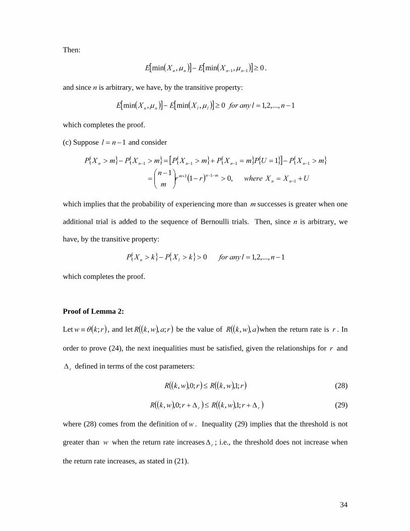
Lemma 2:

Suppose conditions (7) and (8) are satisfied. Let ( )rk;θ be the value of ( )kθ when the return

rate is r . If 5.00 ≤Δ+≤≤ rrr and

5 44.375c c≤ , (20)

then

( ) ( )rrkrk Δ+≥ ;; θθ (21)

Proof: In the Appendix.

Note that the maximum ratio 5 4c c in (20) is a lower bound on the requirement that holds for

states with any number of outstanding items, 2n ≥ . In a practical situation, when n would be

much larger, the inequality imposes no significant constraint on 5 4c c .

Lemma 3:

Let ( )( )( )rwkwnrq l ;0,,, be the value of ( )( )( )0,,, wkwnrq l when the return rate is r . If

0 0.5rr≤ + Δ ≤ then:

( )( )( )( ) ( )( )( )rwkwnrqrwkwrnq lrlr ;0,,,;0,,, ≥Δ+Δ+ (22)

Proof: In the Appendix.

Theorem 2:

Suppose the conditions of Theorem 1 and Lemma 2 are satisfied. Then

( ) ( )( ) ( ) ( )( ) ( ), ; , ,0; , ; , ,0;r r rq n r k r k w r q nr k r k w rθ θ⎡ ⎤ ⎡ ⎤+ Δ + Δ + Δ ≥⎣ ⎦ ⎣ ⎦ .

Proof:

From Lemma 2 we have ( ) ( )rrkrk Δ+≥ ;; θθ , which implies that:

( )( ) ( ) ( )( ) ( ), , , ,0; , ; , ,rq nr k r k w r q nr k r k w rθ θ⎡ ⎤ ⎡ ⎤+ Δ ≥⎣ ⎦ ⎣ ⎦ . (23)

24

From Lemma 3:

( ) ( )( ) ( ) ( )( ) ( ), , , ,0; , ; , ,r r r rq n r k r k w r q nr k r k w rθ θ⎡ ⎤ ⎡ ⎤+ Δ + Δ + Δ ≥ + Δ⎣ ⎦ ⎣ ⎦ . (24)

Then, we have by the transitive property that:

( ) ( )( ) ( ) ( )( ) ( ), , , ,0; , ; , ,r r rq n r k r k w r q nr k r k w rθ θ⎡ ⎤ ⎡ ⎤+ Δ + Δ + Δ ≥⎣ ⎦ ⎣ ⎦ ,

which completes the proof.

Theorem 2 implies that the suitability of the outsourcing option increases when the

return rate increases. This comes not only from the fact that the probability of crossing the

corresponding threshold that determines the optimality of the outsourcing option increases,

but also from the fact that the value for such threshold does not increase.

Then, given that the variability on the return volume increases as the return rate

increases (for any value below 0.5), it can be concluded that outsourcing becomes a more

suitable option for products with greater variability in their return volume.

This conclusion is supported by the fact that (as shown in Lemma 2) in most cases,

the expected reward for 0=a decreases as the return rate, and in consequence the variability

in the return volume, increases. This decrease for the reward when performing RL activities

internally causes the threshold that determines the optimality of the outsourcing option not to

increase. Moreover, as the return rate increases, the threshold may decrease, which expands

the set of states where outsourcing is optimal. This situation will be supported by two

numerical examples that will be shown in the next section.

3.5. Numerical examples.

In order to show the influence of higher variability of the return volume on the suitability of

an outsourcing option, consider a particular scenario defined by the parameters:

25

13121248134

72

61

5

4

3

=========

ccccccWcL

(25)

As well as the sales function:

( )

2 , 1,2,..., 2

2 2 1 , 2 1,...,t

M t t LLs

MM t L t L LL

⎧ =⎪⎪= ⎨⎪ − − − = +⎪⎩

(26)

where 3=M . The values for the cost parameters satisfy conditions (7) to (11) as well as (18);

i.e., there is an optimal monotone nondecreasing policy for any 1≤r .

Table 3 shows the values for the threshold in each set of states, for

{ }5.0,4.0,3.0,2.0=r , as well as the probability ( )( )( )awkwkq ttltt ,,, 1− that such threshold

(defined as lw ) is crossed in each case. These values were obtained by creating a Matlab

program, whose inputs are ,,,,, 21 ccWLr 76543 ,,,, ccccc , as well as the sales volume ts during

the analysis horizon. Based on this information, the program computes the possible states

and orders them according to the criteria defined. The program also computes the amount of

units tn outstanding in the market for each state, as well as the corresponding transition

probabilities and expected costs for 0=a and 1=a . The terminal costs are also obtained.

Based on this, the program solves the MDM by using backward induction, and shows the

optimal action to take at each decision epoch.

Table 3. Value of the threshold and the probability of crossing it for { }0.2,0.3,0.4,0.5r =

26

As it can be identified in Table 3, a greater variability in the return volume (greater r )

increases the probability of crossing the corresponding threshold in each set of states; i.e.,

there is a greater probability that outsourcing ( 1=a ) will be the optimal action to take.

This implies that, as mentioned in section 2.2, greater variability in the return volume

increases the uncertainty about the volume of units put into the corresponding RL system,

which forces the firm to follow an outsourcing strategy, and take advantage of the economies

of scale by involving a 3PRLP in managing returned items.

Now, in order to show the influence of higher variability in the return volume as well

as a shorter product’s life cycle, consider the next two cases:

4,5.0:25,3.0:1

====

LrCaseLrCase

(27)

where both of them are defined by the cost parameters and value for W shown in (25), as well

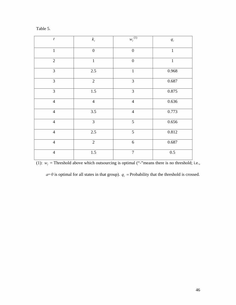
as sales function (26) with 3=M . Tables 4 and 5 show the results for the two cases

considered.

Table 4. Value of the threshold and the probability of crossing it for Case 1: 5,3.0 == Lr

Table 5. Value of the threshold and the probability of crossing it for Case 2: 4,5.0 == Lr

By comparing both cases, it can be identified that when the variability in the return

volume increases and the length of the life cycle decreases, the probability of crossing the

threshold beyond which outsourcing is optimal increases.

These examples with 5.0≤r illustrate how the threshold that determines the

suitability of the outsourcing option for the Markov Decision Model developed is easily

crossed in the scenario where the variability on the return volume is greater (greater r ), and

27

the length L of the product life cycle is shorter. This implies that, due to a high variability in

the rate of returns, it may not be economically feasible for a firm to develop its own RL

facilities, given that the amount of units to be returned will be significantly uncertain over

time, and the required capacity will be changing constantly.

The complexity of this situation increases when the life cycle for this type of products

is extremely short, which requires quick but adequate decisions for these RL systems, in

order to efficiently respond to such changing conditions. This can effectively be

accomplished by involving a 3PRLP, which specializes in these activities, and can take

advantage of the economies of scale to convert RL functions into a profit-creating activity in

the closed-loop chain.

4. Conclusions and Future Work

A Markov Decision Model (MDM) for evaluating an outsourcing option in RL is developed

in this research. It considers several elements that are critical in defining the characteristics of

a RL network, such as the uncertainty in the return volume, the length of the product life

cycle, the sales behavior, the particular RL costs incurred, as well as the length of time

defined for the existence of that RL system. In particular, the length of the product life cycle,

the cost parameters, the sales function defined and the rate of return considered, are modeling

the scenario of interest; i.e., the length of the horizon analysis in the MDM is determined by

such life cycle; while the uncertainty implied in the MDM is represented by the expected

amount of returned units, which is defined by the outstanding units in the market and the rate

of return considered.

The conditions for the existence of an optimal monotone nondecreasing policy were

also shown, where it was verified that such a policy will exist as long as a set of

nonrestrictive assumptions on the cost parameters is satisfied, and the return rate is below a

28

bound defined in terms of those cost parameters. Moreover, there are some instances where

an optimal monotone nondecreasing policy exists, regardless of the value for the return rate.

The existence of an optimal monotone nondecreasing policy implies the presence of a

threshold above which it is optimal to follow an outsourcing strategy for the RL system;

otherwise, to continue performing the RL activities internally. This threshold was defined in

terms of a partial ordering for the system states, where given a fixed capacity at a decision

epoch, the states are ordered according to the cumulative returned units, such that if that

volume goes above a particular level, then it is optimal to follow an outsourcing strategy and

take advantage of the economies of scale implied by involving a 3PRLP in managing the

returns, which has RL as its core function.

It was also shown that outsourcing is a more suitable option for scenarios with greater

variability on the return volume, by explaining analytically the increment in the probability of

crossing the threshold that determines outsourcing optimality when the variability in the

return volume increases. It was also shown how the threshold does not increase when the

return volume variability increases. It may even decrease as such variability increases, which

also increases the probability of crossing it.

As a support to this analysis, two sets of scenarios were explored numerically. In the

first set, the rate of returns was increased while keeping everything else fixed. The results

showed that outsourcing is more suitable when the rate of returns (and in consequence the

variability in the return volume) is greater. The second set contained two different scenarios

with the same cost parameters and sales function, but with different variability in the return

volume and length of the product’s life cycle. In the second scenario, a greater variability and

shorter life cycle existed, and (as expected) outsourcing was a more suitable option in this

scenario than in the first one.

29

4.2. Future Work

Even though the existence of an optimal monotone nondecreasing policy was proved,

the influence on the suitability of the outsourcing option was analytically proved only for the

return volume variability, but not for the length of the product life cycle, whose influence was

shown merely numerically. Developing an analytical proof for the influence of the life cycle

length on outsourcing suitability represents a future research area to consider. The main

challenge for this analysis is the difference in the cardinality of the sets of ordered states

obtained for each case. This comes from the fact that the size of the state space at each

decision epoch is determined by the sales function of the product analyzed, as well as the

length of the lifecycle.

Finally, future research can also consider various extensions to this model. Several

problem parameters, such as the rate of returns and/or the RL costs may not be constant

during the product’s life cycle. Nonstationary costs will be easy to incorporate, but variation

in the return rate will require more elaborate modifications to the analysis. More generally,

another area of research would identify the requirements for the existence of an optimal

monotone nondecreasing policy, when the returns follow a probability distribution different

than the one described in this paper. The influence of a different stochastic behavior for the

returns (according to a particular scenario of interest) can be considered, which will represent

the basis for evaluating the five conditions required for such a policy structure.

A full analysis of the outsourcing decision should also consider the possibility that

internal management does not imply that the RL capacity is adjusted to the expected returns,

either because the firm does not have the capability of adjusting its capacity each period, or

because a different adjustment policy is found to result in better performance. The

irreversibility of the outsourcing decision assumed in this paper also could be relaxed, in

view of the fact that the 3PRLP selected may fail to perform adequately. Finally, the potential

30

for profits from reprocessing and selling returned items may be considered as a benefit of

maintaining RL capacity internally.

References

1. Bufardi, A. et.al. “Multicriteria decision-aid approach for product end-of-life alternative

selection”. International Journal of Production Research. Vol. 42. Iss. 16. p. 3139. 2004.

2. Dowlatshahi, S. “Developing a Theory of Reverse Logistics”. Interfaces. Vol. 30. No. 3.

pp. 143-155. 2000.

3. Dowlatshahi, S. “A strategic framework for the design and implementation of

remanufacturing operations in reverse logistics”. International Journal of Production

Research. Vol. 43. Iss. 16. p. 3455. 2005.

4. Gonzalez, B., Adenso-Diaz, B. “A bill of materials-based approach for end-of-life

decision making in design for the environment”. International Journal of Production

Research. Vol. 43. Iss. 10. p. 2071. 2005.

5. Guide, D. R. and van Wassenhove, L. N. “Business Aspects of Closed-Loop Supply

Chains”, in Business Aspects of Closed-Loop Supply Chains. Exploring the issues. pp.

17-42. 2003.

6. Krumwiede, D. W. and Sheu, C. “A model for reverse logistics entry by third-party

providers”. The International Journal of Management Sciences. Vol. 30. pp. 325-333.

2002.

7. Meade, L., Sarkis, J. “A conceptual model for selecting and evaluating third-party reverse

logistics providers”. Supply Chain Management: An International Journal. Vol. 7. No. 5.

pp. 283-295. 2002.

8. Nakashima, K, et.al. “Optimal Control of a remanufacturing system”. International

Journal of Production Research. Vol. 42. Iss. 17. p. 3619. 2004.

31

9. Puterman, M. L. Markov Decision Processes. Discrete Stochastic, Dynamic

Programming. Wiley Series in Probability and Mathematical Statistics. John Wiley &

Sons. Canada. 1994.

10. Razzaque, M. A., and Sheng, C.C. “Outsourcing of logistics functions: a literature

survey”. International Journal of Physical Distribution & Logistics Management. Vol. 28.

No. 2. pp. 89-107. 1998.

11. Rogers, D. S., R. S. Tibben-Lembke. Going Backwards: Reverse Logistics Trends and

Practices. Reverse Logistics Executive Council. 1999.

12. Shaked, M., Shanthikumar, J. G. Stochastic Orders and Their Applications. Academic

Press. 1994.

13. Serrato, M. Outsourcing Analysis for Reverse Logistics Systems: A Qualitative Study &

a Markov Decision Model. Unpublished Ph.D. Dissertation, Iowa State University, 2006.

14. Stock, J. R. Development and implementation of Reverse Logistics Programs. 1998.

Council of Logistics Management. Oak Brook, IL.

15. Tang, O., et.al. “Economic evaluation of disassembly processes in remanufacturing

systems”. International Journal of Production Research. Vol. 42. Iss. 17. p. 3603. 2004.

16. Tibben-Lembke, R. S. “Life after death: reverse logistics and the product life cycle”.

International Journal of Physical Distribution & Logistics Management. Vol. 32. No. 3.

pp. 223-244. 2002.

17. Toktay, B. “Forecasting Product Returns”, in Business Aspects of Closed-Loop Supply

Chains. Exploring the issues. pp. 203-220. 2003.

18. Vaidyanathan, J. “Production planning for closed-loop supply chains with recovery and

reuse: an analytical approach”. International Journal of Production Research. Vol. 44. Iss.

5. p. 981. 2006.

32

19. Willems, B. et.al. “Can large-scale disassembly be profitable? A linear programming

approach to quantifying the turning point to make disassembly economically viable”.

International Journal of Production Research. Vol. 44. Iss. 6. p. 1125. 2006.

20. Wu, F, et.al. “An outsourcing model for sustaining long-term performance”. International

Journal of Production Research. Vol. 43. Iss. 12. p. 2513. 2005.

APPENDIX

Proof of Lemma 1.

(a) Suppose 1−= nl and consider

( ) ( )( ) ( ) ( )( )1 1 1

1

n n n n n

n n

E X nr X nr r E E X nr X nr r X

where X X U

++ + +− − −

−

⎡ ⎤⎡ ⎤ ⎡ ⎤− − − − = − − − −⎢ ⎥⎢ ⎥ ⎢ ⎥⎣ ⎦⎣ ⎦ ⎣ ⎦= +

where U = 1 with probability r and 0 otherwise. There are three possible cases for 1nX m− = ,

which are shown in Table 6.

Table 6. Cases considered for Case (a) in Lemma 1.

In the first case, ( ) ( )( ) ( )1 1 1n n nE X nr X nr r X m r m nr+ + +− −

⎡ ⎤− − − − = = + −⎢ ⎥⎣ ⎦ given that

nr>m. Then, this case yields a nonnegative result. In the second case,

( ) ( )( ) ( )( )1 1 1n n nE X nr X nr r X m nr m r++

− −⎡ ⎤− − − − = = − −⎢ ⎥⎣ ⎦

where, given that nr>m, the expression is also nonnegative. Finally, for the third case,

( ) ( )( ) 0n lE X nr E X nr r++ ⎡ ⎤⎡ ⎤− − − − =⎢ ⎥⎣ ⎦ ⎣ ⎦

, given that nrm ≥ . Then, to complete the conditioning

argument:

33

( ) ( )( )

( ) ( )( )

( ) ( )( ) ( )

1

1 1

1

1 1 10

0.

n n

n n n

n

n n n nm

E X nr E X nr r

E E X nr X nr r X

E X nr X nr r X m P X m

++−

++− −

− ++− − −

=

⎡ ⎤⎡ ⎤− − − −⎢ ⎥⎣ ⎦ ⎣ ⎦⎡ ⎤⎡ ⎤= − − − −⎢ ⎥⎢ ⎥⎣ ⎦⎣ ⎦

⎡ ⎤= − − − − = = ≥⎢ ⎥⎣ ⎦∑

Then, considering that ( ) ( )1 1 0n n n nE X E Xμ μ+ +− −

⎡ ⎤ ⎡ ⎤− − − ≥⎣ ⎦ ⎣ ⎦ and, since n is arbitrary, we

have, by the transitive property:

( ) ( ) 0 1, 2,... 1n n l lE X E X for any l nμ μ+ +⎡ ⎤ ⎡ ⎤− − − ≥ = −⎣ ⎦ ⎣ ⎦

which completes the proof.

(b) Suppose 1−= nl and consider

( ) ( )( )[ ] ( ) ( )( )[ ][ ]UXXwhere

XrnrXnrXEErnrXnrXE

nn

nnnnn

+=

−−=−−

−

−−−

1

111 ,min,min,,min

where U = 1 with probability r and 0 otherwise. Suppose rnrmX n −<=−1 . Then

( ) ( )( ) ( ) ( )1 1min , min , min 1, 1n n nE X nr X nr r X m r m nr r m m− −⎡ ⎤− − = = + + − −⎣ ⎦

since nrmirnrm <⇒−< . Also, ( ) rmnrmrmnr +≥+⇒+> ,1min , so

( ) ( ) ( ) ( ) 211,1min rmmrrmrmmrnrmr =−−++≥−−++ .

On the other hand, suppose rnrmX n −≥=−1 . Then

( ) ( )( ) ( ) ( )1 1min , min , 1 min ,n n nE X nr X nr r X m rnr r m nr nr r− −⎡ ⎤− − = == + − − +⎣ ⎦

because nrmrnrm ≥+⇒−≥ 1 . Also, ( ) rnrnrm −≥,min , which implies that

( ) ( ) ( )( ) 22 1,min1 rrnrrnrrnrrnrnrmrrnr =+−−−+≥+−−+ .

To complete the conditioning argument:

( ) ( )( ) ( )

( ) ( ) ( )1

0

min , min ,

min , min ,

min , min , 0

n l

n l l

n

n l l lm

E X nr X nr r

E E X nr X nr r X

E X nr X nr r X m P X m−

=

⎡ ⎤− −⎣ ⎦⎡ ⎤⎡ ⎤= − −⎣ ⎦⎣ ⎦

⎡ ⎤= − − = = ≥⎣ ⎦∑

34

Then:

( )[ ] ( )[ ] 0,min,min 11 ≥− −− nnnn XEXE μμ .

and since n is arbitrary, we have, by the transitive property:

( )[ ] ( )[ ] 1,...,2,10,min,min −=≥− nlanyforXEXE llnn μμ

which completes the proof.

(c) Suppose 1−= nl and consider

{ } { } { } { } { }[ ] { }

( ) UXXwhererrm

nmXPUPmXPmXPmXPmXP

nnmnm

nnnnn

+=>−⎟⎟⎠

⎞⎜⎜⎝

⎛ −=

>−==+>=>−>

−−−+

−−−−

111

1111

,011

1

which implies that the probability of experiencing more than m successes is greater when one

additional trial is added to the sequence of Bernoulli trials. Then, since n is arbitrary, we

have, by the transitive property:

{ } { } 1,...,2,10 −=>>−> nlanyforkXPkXP ln

which completes the proof.

Proof of Lemma 2:

Let ( )rkw ;θ≡ , and let ( )( )rawkR ;,, be the value of ( )( )awkR ,, when the return rate is r . In

order to prove (24), the next inequalities must be satisfied, given the relationships for r and

rΔ defined in terms of the cost parameters:

( )( ) ( )( )rwkRrwkR ;1,,;0,, ≤ (28)

( )( ) ( )( )rr rwkRrwkR Δ+≤Δ+ ;1,,;0,, (29)

where (28) comes from the definition of w . Inequality (29) implies that the threshold is not

greater than w when the return rate increases rΔ ; i.e., the threshold does not increase when

the return rate increases, as stated in (21).

35

Given that by definition of w , inequality (28) is satisfied, and that the right-hand sides in both

inequalities are equal (they do not depend on r ), inequality (29) will be satisfied as long as:

( )( ) ( )( )rwkRrwkR r ;0,,;0,, ≤Δ+ , (30)

where (30) can be rewritten as:

( )( ) ( )( ) ( )( ) ( )( )( )( )( ) ( )( )( )( )( )( ) ( )( )( ) ( )

( )

1 2 3

4 1 2

5 1 2 1

2

min , min ,

max ,0 max ,0 0 where , ,

,

r r r

r

r r

c n r k nr k c k n r k nr c n

c E x n r E x nr

c E x n r E x nr x Bin n r

x Bin n r

+ ++ ++ Δ − − − + − + Δ − − + Δ

+ + Δ −

+ − + Δ − − > + Δ∼

∼

(31)

where, given (7) and (8), the following part of (31) is nonnegative:

( )( ) ( )( ) ( )( ) ( )( ) 0321 ≥Δ+−−Δ+−+−−−Δ+ ++++rrr ncnrkrnkcknrkrnc

Consider the rest of the elements of 31):

( )( )( ) ( )( )( )( )( )( ) ( )( )( )0,max0,max

,min,min

215

214

nrxErnxEcnrxErnxEc

r

r

−−Δ+−+−Δ+

(32)

Let ( ) ( )min ,ng r E X nr= ⎡ ⎤⎣ ⎦ and ( ) ( )max ,0nf r E X nr= −⎡ ⎤⎣ ⎦ where ( )binomial ,X n r∼

and 2n ≥ . Then, (32) will be true if the combined cost function ( ) ( )4 5n nc g r c f r+ is an

increasing function of r.

The derivatives of fn and gn are discontinuous at r = j/n, j = 1, …, n-1, which implies that a

separate expression is needed for the derivatives in each interval for r. For

1, or equivalently 1,j jr j nr jn n

+< ≤ < ≤ + where 2 j n< :

( ) ( ) ( ) ( ) ( )

( ) ( ) ( ) ( ) ( )

1 0

1 1 0

and

jn

nk j k

j jn

nk k j k

f r k nr p k nr k p k

g r kp k nr p k nr nr k p k

= + =

= = + =

= − = −

= + = − −

∑ ∑

∑ ∑ ∑

36

where ( ) ( )1 n kknp k r r

k−⎛ ⎞

= −⎜ ⎟⎝ ⎠

. Then

( ) ( ) ( ) ( ) ( ) ( )

( ) ( ) ( )

4 5 4 50 0

4 5 40

.

j j

n nk k

j

k

c g r c f r c nr nr k p k c nr k p k

c nr c c nr k p k

= =

=

⎛ ⎞ ⎛ ⎞+ = − − + −⎜ ⎟ ⎜ ⎟

⎝ ⎠ ⎝ ⎠

= + − −

∑ ∑

∑

We wish to show that ( ) ( )( )4 5 0n nc g r c f rr∂

+ ≥∂

for reasonable values of 4 5c c< .

(a) ( ) ( ) ( ) ( ) ( )1

01 1 1 1

jn k n jk j

k

n nnr k r r n j r r j n r

k jr− − −

=

⎛ ⎞ ⎛ ⎞∂− − = − − + − +⎡ ⎤⎜ ⎟ ⎜ ⎟ ⎣ ⎦∂ ⎝ ⎠ ⎝ ⎠

∑

The proof is inductive, using integration by parts. First, for j = 0, or equivalently, 0 1nr< ≤ ,

integrating by parts with ( )1 1u n r= − + and ( ) 11 ndv n r dr−= − we get:

( ) ( ) ( ) ( ) ( )( )

( ) ( ) ( ) ( )

1

1

1 1 1 1 1 1 1 1

1 1 1 1 1 .

n n n

n n n

n r n r dr n r r n r dr

n r r r nr r

−

+

⎡ ⎤ ⎡ ⎤− − + = − − + − − + −⎣ ⎦ ⎣ ⎦

⎡ ⎤= − − + − + − = −⎣ ⎦

∫ ∫

And for j = 1, or equivalently, 1 2nr< ≤ ,

( )( ) ( ) ( ) ( ) ( ) ( )

[ ]( ) ( )( ) ( ) ( )

2 1 12 2

1

1

1 1 2 1 2 1 1 2 1 1 1

1 1 1 2 1

1 1 1 ,

n n n

n n

n n

n n r r n r dr n r n r r n r n r dr

nr nr r r nr r

nr r nr nr r

− − −

−

−

⎡ ⎤ ⎡ ⎤ ⎡ ⎤− − − + = − − + − + − − +⎣ ⎦⎣ ⎦ ⎣ ⎦

= − − + − − + −

= − + − −

∫ ∫

where the second equality results from substituting for the j = 0 integral.

Now, for j > 1, assume:

( )( ) ( ) ( ) ( )1

1

01 1 1 1

1

jn j n kj j k

k

n nn j r jr n r dr nr k r r

j k

−− −−

=

⎛ ⎞ ⎛ ⎞⎡ ⎤− + − − + = − −⎜ ⎟ ⎜ ⎟⎣ ⎦−⎝ ⎠ ⎝ ⎠∑∫ .

Then:

37

( )( ) ( ) ( )

( ) ( ) ( ) ( ) ( ) ( )

[ ]( ) ( )( ) ( )

( ) ( )

1 1

1

1

1 1 1

1 1 1 1 1 1

11 1 1 1 11

1

n j j j

n j n jj j j

n j n jj j j

n jj

nn j r j r n r dr

j

n nr j n r r j r jr n r dr

j j

n njr j nr r r n j r jr n r drj jj

n nnr j r r

j j

− − +

− − −

− − −

−

⎛ ⎞ ⎡ ⎤− − + − +⎜ ⎟ ⎣ ⎦⎝ ⎠⎛ ⎞ ⎛ ⎞ ⎡ ⎤= − + − + − + + − − +⎡ ⎤⎜ ⎟ ⎜ ⎟⎣ ⎦ ⎣ ⎦⎝ ⎠ ⎝ ⎠⎛ ⎞ ⎛ ⎞+ ⎡ ⎤= − − + − − + − + − − +⎜ ⎟ ⎜ ⎟ ⎣ ⎦−⎝ ⎠ ⎝ ⎠

⎛ ⎞ ⎛= − − −⎜ ⎟⎝ ⎠

∫

∫

∫

( ) ( ) ( )

( ) ( ) ( ) ( ) ( )

11

0

11

0 0

11 1

11 1 1

jn j n kj k

k

j jn k n j n kk j k

k k

njr r nr k r rkj

n n nnr k r r r r nr k r r

k j kj

−− + −

=

−− − + −

= =

⎞ ⎛ ⎞+− + − −⎜ ⎟ ⎜ ⎟

⎝ ⎠ ⎝ ⎠⎛ ⎞ ⎛ ⎞ ⎛ ⎞

= − − − − + − −⎜ ⎟ ⎜ ⎟ ⎜ ⎟⎝ ⎠ ⎝ ⎠ ⎝ ⎠

∑

∑ ∑

( ) ( ) ( ) ( )1

1

0 01 , if 1

j jn k j kk j k

k k

n n nnr k r r j r nr k r r

k j k

−− − −

= =

⎛ ⎞ ⎛ ⎞ ⎛ ⎞= − − = − −⎜ ⎟ ⎜ ⎟ ⎜ ⎟

⎝ ⎠ ⎝ ⎠ ⎝ ⎠∑ ∑ .

(b) To show: ( ) ( )1

1

01

jj kj k

k

n nj r nr k r r

j k

−− −

=

⎛ ⎞ ⎛ ⎞= − −⎜ ⎟ ⎜ ⎟

⎝ ⎠ ⎝ ⎠∑ . This is equivalent to:

( ) ( ) ( ) ( ) ( )1

1

01 1 1 ! 1

jj kj k

k

nn n n j r j nr k r r

k

−− −

=

⎛ ⎞− − + = − − −⎜ ⎟

⎝ ⎠∑

and can be verified for j = 1 and j = 2. Then for j > 2, assume the equality is true for j – 1 as

above. For j,

( ) ( ) ( ) ( ) ( )

( ) ( ) ( ) ( ) ( ) ( )

( ) ( ) ( ) ( ) ( ) ( )( ) ( )

1

0 0

11

0

1

! 1 ! 1

! 1 1 1 1

1 1 1 1 1

1

j jj k j kk k j

k k

jj kk j

k

j j

j

n n nj nr k r r j nr k r r nr j r

k k j

nj r nr k r r nr j n n n j r

k

j r n n n j r nr j n n n j r

n n n j r

−− −

= =

−− −

=

+

⎡ ⎤⎛ ⎞ ⎛ ⎞ ⎛ ⎞− − = − − + −⎢ ⎥⎜ ⎟ ⎜ ⎟ ⎜ ⎟

⎝ ⎠ ⎝ ⎠ ⎝ ⎠⎣ ⎦⎛ ⎞

= − − − + − − − +⎜ ⎟⎝ ⎠

= − − − + + − − − +

= − −

∑ ∑

∑

This completes the proof of (a).

(c) Using (a), for 1, or equivalently 1,j jr j nr jn n

+< ≤ < ≤ +

( ) ( ) ( ) ( ) ( )

( ) ( ) ( ) ( ) ( ) ( )

4 5 4 5 40

14 5 4 4 5 41 1 1 , , .

j

n nk

n jj

c g r c f r c nr c c nr k p kr r

nc n c c n j r r j n r c n c c j n r

jφ

=

− −

⎡ ⎤∂ ∂+ = + − −⎡ ⎤ ⎢ ⎥⎣ ⎦∂ ∂ ⎣ ⎦

⎛ ⎞= + − − − + − + ≡ + −⎡ ⎤⎜ ⎟ ⎣ ⎦

⎝ ⎠

∑

38

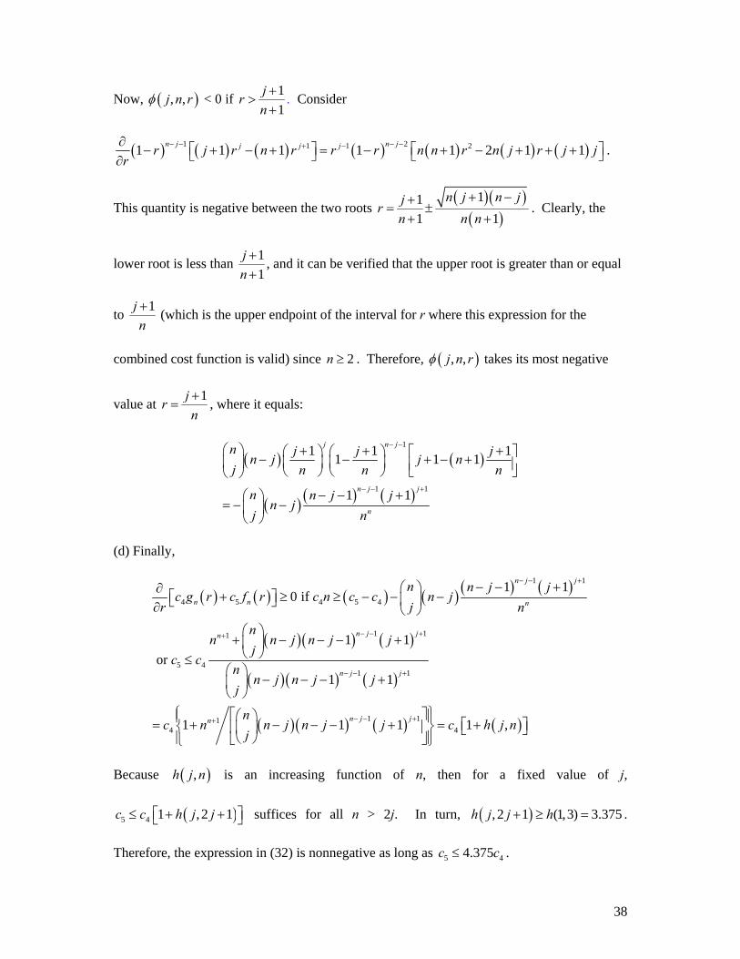
Now, ( ), ,j n rφ < 0 if 11

jrn+

>+

. Consider

( ) ( ) ( ) ( ) ( ) ( ) ( )1 21 1 21 1 1 1 1 2 1 1n j n jj j jr j r n r r r n n r n j r j jr

− − − −+ −∂ ⎡ ⎤ ⎡ ⎤− + − + = − + − + + +⎣ ⎦ ⎣ ⎦∂.

This quantity is negative between the two roots ( )( )

( )11

1 1n j n jjr

n n n+ −+

= ±+ +

. Clearly, the

lower root is less than 11

jn++

, and it can be verified that the upper root is greater than or equal

to 1jn+ (which is the upper endpoint of the interval for r where this expression for the

combined cost function is valid) since 2n ≥ . Therefore, ( ), ,j n rφ takes its most negative

value at 1jrn+

= , where it equals:

( ) ( )

( ) ( ) ( )

1

1 1

1 1 11 1 1

1 1

j n j

n j j

n

n j j jn j j nj n n n

n n j jn j

j n

− −

− − +

⎛ ⎞ + + +⎛ ⎞ ⎛ ⎞ ⎡ ⎤− − + − +⎜ ⎟ ⎜ ⎟ ⎜ ⎟ ⎢ ⎥⎝ ⎠ ⎝ ⎠ ⎣ ⎦⎝ ⎠

− − +⎛ ⎞= − −⎜ ⎟

⎝ ⎠

(d) Finally,

( ) ( ) ( ) ( ) ( ) ( )

( )( ) ( )

( )( ) ( )

( )( ) ( ) ( )

1 1

4 5 4 5 4

1 11

5 41 1

1 114 4

1 10 if

1 1 or

1 1

1 1 1 1 ,

n j j

n n n

n j jn

n j j

n j jn

n n j jc g r c f r c n c c n j

jr n

nn n j n j j

jc c

nn j n j j

j

nc n n j n j j c h j n

j

− − +

− − ++

− − +

− − ++

− − +⎛ ⎞∂+ ≥ ≥ − − −⎡ ⎤ ⎜ ⎟⎣ ⎦∂ ⎝ ⎠

⎛ ⎞+ − − − +⎜ ⎟⎝ ⎠≤

⎛ ⎞− − − +⎜ ⎟

⎝ ⎠⎧ ⎫⎡ ⎤⎛ ⎞⎪ ⎪= + − − − + = +⎡ ⎤⎨ ⎬⎢ ⎥⎜ ⎟ ⎣ ⎦

⎝ ⎠⎪ ⎪⎣ ⎦⎩ ⎭

Because ( ),h j n is an increasing function of n, then for a fixed value of j,

( )5 4 1 ,2 1c c h j j⎡ ⎤≤ + +⎣ ⎦ suffices for all n > 2j. In turn, ( ), 2 1 (1,3) 3.375h j j h+ ≥ = .

Therefore, the expression in (32) is nonnegative as long as 5 44.375c c≤ .

39

This completes the proof.

Proof of Lemma 3:

Inequality (22) can be rewritten as:

( ) ( ) ( )∑ ∑= =

−− −⎟⎟⎠

⎞⎜⎜⎝

⎛≥Δ−−Δ+⎟⎟

⎠

⎞⎜⎜⎝

⎛n

wj

n

wj

jnjjnr

jr

l l

rrjn

rrjn

11

which is equivalent to:

{ } { } { }nwforwxPwxP lll ,...,2,111 21 =−>≥−> (33)

where 1x is binomial with parameters n and rr Δ+ and 2x is binomial with parameters n and

r . The result follows from the fact that the family of binomial distributions for fixed n is

stochastically increasing in r (Shaked and Shanthikumar, 1994).

40

Figure 1.

Re -Use

Supply Production Distribution

Collection Selection Re-Processing

Re-Distribution

Disposal

Use

Flow of goods in RL chain

Flow of goods in “forward” chain

Known variable (at a certain degree)

Unknown variable

Third Party Reverse Logistics Provider Facilities

a=0

RL Facilities

3PRLP

RL as core activity = no shortages, manages all future returns

Which capacity level is optimal? How to adjust such capacity?

What happens if returns are greater than capacity developed?=shortages

c1, c2, c3

c5

c6

a=1 Shortages

Dispose RL firm’s capacity

c7

c4

41

Figure 2.

( )tf

t wk ,

( )1, +tf

t wk

( )2, +tf

t wk

( )3, +tf

t wk

( )tgt wk ,1+

( )1,1 ++ tgt wk

( )2,1 ++ tgt wk

( )1,1 ++ tht wk

( )2,1 ++ tht wk

( )3,1 ++ tht wk

= States grouped for kt and ordered according to wt. Recall that some states may have several predecessors

42

Table 1.

Case Value on the right-

hand side of the

inequality

Resulting inequality in the worst

case:

( )rinYrnX tt −>> ,)1.1

( )irYXcirc −−+ 54

Worst case:

iYX =−

( ) ( )rccrcccc 452357 −−−≥−

( )rinYrnX tt −≤> ,)2.1

( ) YcXcccrnt 4554 −+− Worst case:

iirnrXirnrY

+−=−= ,

Because 45 cc ≥

( ) ( )rccrcccc 452357 −−−≥−

( )rinYrnX tt −≤≤ ,)3.1 ( )YXc −4

Worst case:

iYX =−

( )rcccc 2347 −≥−

( )rinYrnX tt −>≤ ,)4.1

( )( )545

445

ccirYcXcccrnt

−+−+−

Worst case:

( )rnX

rinY

t

t

=−= ,

( )rccrcc 2347 −≥−

43

Table 2.

Case Value on the right-

hand side of the

inequality

Resulting inequality in the worst

case:

( )rinYrnX tt −>> ,)1.1

( )irYXcirc −−+ 54

Worst case:

iYX =−

( ) ( )rccrcccc 453157 −−+≥−

( )rinYrnX tt −≤> ,)2.1

( ) YcXcccrnt 4554 −+− Worst case:

iirnrXirnrY

+−=−= ,

Because 54 cc <

( ) ( )rccrcccc 453157 −−+≥−

( )rinYrnX tt −≤≤ ,)3.1 ( )YXc −4

Worst case:

iYX =−

( )rcccc 3147 +≥−

( )rinYrnX tt −>≤ ,)4.1

( )( )545

445

ccirYcXcccrnt

−+−+−

Worst case:

( )rnX

rinY

t

t

=−= ,

( )rccrcc 3147 +≥−

44

Table 3.

2.0=r 3.0=r 4.0=r 5.0=r

t States tk lw (1) tq lw tq lw tq lw tq

1 0r - 0 - 0 - 0 0 1

2 2r - 0 - 0 - 0 0 1

3 5r - 0 - 0 5 0.0124 1 0.922

3 4r - 0 - 0 - 0 3 0.524

3 3r - 0 - 0 - 0 3 0.784

4 8r - 0 8 0.0006 6 0.049 4 0.405

4 7r - 0 - 0 7 0.188 4 0.580

4 6r - 0 - 0 7 0.040 5 0.455

4 5r - 0 - 0 8 0.010 5 0.663

4 4r - 0 - 0 8 0.025 6 0.524

4 3r - 0 - 0 8 0.064 7 0.352

(1) lw = Threshold above which outsourcing is optimal (“-”means there is no threshold; i.e.,

a=0 is optimal for all states in that group). =tq Probability that the threshold is crossed.

45

Table 4.

t tk lw (1) tq

1 0 - 0

2 0.3 - 0

3 0.9 - 0

3 0.6 - 0

4 2.1 7 0.0002

4 1.8 7 0.0007

4 1.5 - 0

4 1.2 - 0

5 2.7 8 0.0004

5 2.4 8 0.0012

5 2.1 9 0.0002

5 1.8 9 0.0007

5 1.5 9 0.002

5 1.2 9 0.0081

5 0.9 9 0.027

5 0.6 - 0

(1): lw =Threshold above which outsourcing is optimal (“-”means there is no threshold; i.e.,

a=0 is optimal for all states in that group). =tq Probability that the threshold is crossed.

46

Table 5.

t tk lw (1) tq

1 0 0 1

2 1 0 1

3 2.5 1 0.968

3 2 3 0.687

3 1.5 3 0.875

4 4 4 0.636

4 3.5 4 0.773

4 3 5 0.656

4 2.5 5 0.812

4 2 6 0.687

4 1.5 7 0.5

(1): lw = Threshold above which outsourcing is optimal (“-”means there is no threshold; i.e.,

a=0 is optimal for all states in that group). =tq Probability that the threshold is crossed.

47

Table 6.

Case Conditioning argument

1 rnrm −<

2 nrmrnr <≤−

3 mnr ≤

48

Captions for Figures and Tables:

Figure 1. Relationship between RL chain and costs considered in the MDM.

Figure 2. Criterion followed for a strict partial state ordering.

Table 1. Cases for Condition 3 when tr krn <

Table 2. Cases for Condition 3 when ( )rink tt −≤

Table 3. Value of the threshold and the probability of crossing it for { }0.2,0.3,0.4,0.5r =

Table 4. Value of the threshold and the probability of crossing it for Case 1: 5,3.0 == Lr

Table 5. Value of the threshold and the probability of crossing it for Case 2: 4,5.0 == Lr

Table 6. Cases considered for Case (a) in Lemma 1.