A Low Order Finite ElementMethod for Poroelasticity withApplications to Lung Modelling

Lorenz Berger

Keble College

University of Oxford

A thesis submitted for the degree of

Doctor of Philosophy

Trinity Term 2015

Abstract

In the last few decades modelling deformation and flow in porous media has been

of great interest due to its application in various fields including biomechanics,

soil mechanics, geophysics, physical chemistry and material sciences. Particularly

in biology, virtually any application of poroelasticity implies the use of nonlinear

constitutive models, irregular three-dimensional geometries, complicated bound-

ary conditions and jumps in material coefficients, characteristics that can only

be simulated numerically.

In this thesis we develop a stabilised finite element method for solving the

equations of poroelasticity to enable solving complex models of biological tissues

such as the human lungs. For the proposed numerical scheme, we use the lowest

possible approximation order: piecewise constant approximation for the pres-

sure, and piecewise linear continuous elements for the displacements and fluid

flux. Due to the discontinuous pressure approximation, sharp pressure gradi-

ents due to changes in material coefficients or boundary layer solutions can be

captured reliably. We begin by developing theoretical results for approximating

the linear poroelastic equations valid in small deformations. In particular, we

prove existence and uniqueness, an energy estimate and an optimal a-priori error

estimate for the discretised problem. We then extend this work and construct a

stabilised finite element method to solve the poroelastic equations valid in large

deformations. We present the linearisation and discretisation for this nonlinear

problem, and give a detailed account of the implementation. We rigorously test

both the linear and nonlinear finite element method using numerous test prob-

lems to verify theoretical stability and convergence results, and the method’s

ability to reliably capture steep pressure gradients.

Finally, we derive a poroelastic model for lung parenchyma coupled to an

airway fluid network model, and develop a stable method to solve the coupled

i

model. Numerical simulations, on a realistic lung geometry, illustrate the cou-

pling between the poroelastic medium and the network flow model, and simu-

lations of tidal breathing are shown to reproduce global physiologically realistic

measurements. We also investigate the effect of airway constriction and tissue

weakening on the ventilation, tissue stress and alveolar pressure distribution.

ii

Publications

Below are a list of publications which directly relate to the work described in

this thesis.

• L. Berger, R. Bordas, D. Kay, and S. Tavener; Stabilized low-order finite

element approximation for linear three-field poroelasticity SIAM Journal

on Scientific Computing (Under Review)

• L. Berger, R. Bordas, D. Kay, and S. Tavener; A stabilized finite ele-

ment method for nonlinear poroelasticity Computer Methods in Applied

Mechanics and Engineering (Under Review)

• L. Berger, R. Bordas, K. Burrowes, V. Grau, D. Kay; A poroelastic model

coupled to a fluid network with applications in lung modelling International

Journal for Numerical Methods in Biomedical Engineering (Under Review)

iii

Conference Presentations

The work described in this thesis was presented at the following international

conferences:

• L. Berger, R. Bordas, K. Burrowes, C. Brightling, R. Hartley, D. Kay; Un-

derstanding The Interdependence Between Parenchymal Deformation And

Ventilation In Obstructive Lung Disease, The American Thoracic Society

conference, San Diego, May 2014. (Poster)

• L. Berger, R. Bordas, D. Kay; Solving the Generalised Large Deformation

Poroelastic Equations for Modelling Tissue Deformation and Ventilation

in the Lung, European Numerical Mathematics and Advanced Applications

conference, EPFL, Lausanne, August 2013. (Oral)

iv

Contents

1 Introduction 11.1 Poroelastic models in biology . . . . . . . . . . . . . . . . . . . . 21.2 Numerical challenges . . . . . . . . . . . . . . . . . . . . . . . . . 31.3 Thesis goals . . . . . . . . . . . . . . . . . . . . . . . . . . . . . . 41.4 Thesis structure . . . . . . . . . . . . . . . . . . . . . . . . . . . . 5

2 Poroelasticity theory 72.1 Kinematics . . . . . . . . . . . . . . . . . . . . . . . . . . . . . . 72.2 Volume fractions . . . . . . . . . . . . . . . . . . . . . . . . . . . 112.3 Conservation of mass . . . . . . . . . . . . . . . . . . . . . . . . . 122.4 Conservation of momentum . . . . . . . . . . . . . . . . . . . . . 132.5 Constitutive relations . . . . . . . . . . . . . . . . . . . . . . . . . 142.6 Summary of the general poroelasticity model . . . . . . . . . . . . 162.7 Simplification and reformulation of the model . . . . . . . . . . . 172.8 Linear poroelasticity . . . . . . . . . . . . . . . . . . . . . . . . . 18

3 Finite element method 213.1 Introduction . . . . . . . . . . . . . . . . . . . . . . . . . . . . . . 213.2 Norms and spaces . . . . . . . . . . . . . . . . . . . . . . . . . . . 223.3 Model problem . . . . . . . . . . . . . . . . . . . . . . . . . . . . 24

3.3.1 Weak formulation . . . . . . . . . . . . . . . . . . . . . . . 253.3.2 Time discretisation . . . . . . . . . . . . . . . . . . . . . . 263.3.3 Spatial finite element discretisation . . . . . . . . . . . . . 26

3.4 Mixed methods . . . . . . . . . . . . . . . . . . . . . . . . . . . . 283.5 Poroelastic finite element discretisations . . . . . . . . . . . . . . 32

3.5.1 Linear discretisations . . . . . . . . . . . . . . . . . . . . . 323.5.2 Discretisations valid in large deformations . . . . . . . . . 34

4 A stabilised finite element method for linear poroelasticity 354.1 Introduction . . . . . . . . . . . . . . . . . . . . . . . . . . . . . . 354.2 The poroelastic model . . . . . . . . . . . . . . . . . . . . . . . . 36

4.2.1 Governing equations . . . . . . . . . . . . . . . . . . . . . 364.2.2 Weak formulation . . . . . . . . . . . . . . . . . . . . . . . 374.2.3 Fully-discrete model . . . . . . . . . . . . . . . . . . . . . 39

4.3 Norms and inequalities . . . . . . . . . . . . . . . . . . . . . . . . 40

v

4.3.1 Useful inequalities . . . . . . . . . . . . . . . . . . . . . . 404.3.2 Properties of the J-norm . . . . . . . . . . . . . . . . . . . 414.3.3 Approximation results . . . . . . . . . . . . . . . . . . . . 424.3.4 Triple-norms . . . . . . . . . . . . . . . . . . . . . . . . . . 44

4.4 Existence and uniqueness of solutions to the fully-discrete model . 444.5 Energy estimate for the fully-discrete model . . . . . . . . . . . . 49

4.5.1 Bound on the displacement, fluid flux and pressure . . . . 504.5.2 Bound on the divergence of the fluid flux . . . . . . . . . . 534.5.3 The energy estimate . . . . . . . . . . . . . . . . . . . . . 57

4.6 A-priori error analysis . . . . . . . . . . . . . . . . . . . . . . . . 574.6.1 Galerkin orthogonality . . . . . . . . . . . . . . . . . . . . 584.6.2 Auxiliary error estimates . . . . . . . . . . . . . . . . . . . 594.6.3 The a-priori error estimate . . . . . . . . . . . . . . . . . . 64

4.7 Implementation . . . . . . . . . . . . . . . . . . . . . . . . . . . . 654.7.1 Algorithm to assemble the stabilisation matrix . . . . . . . 66

4.8 Numerical Results . . . . . . . . . . . . . . . . . . . . . . . . . . . 664.8.1 2D test problem . . . . . . . . . . . . . . . . . . . . . . . . 674.8.2 3D test problem . . . . . . . . . . . . . . . . . . . . . . . . 704.8.3 2D cantilever bracket problem . . . . . . . . . . . . . . . . 724.8.4 3D unconfined compression stress relaxation . . . . . . . . 73

4.9 Conclusion . . . . . . . . . . . . . . . . . . . . . . . . . . . . . . . 76

5 A stabilised finite element method for poroelasticity valid inlarge deformations 775.1 Introduction . . . . . . . . . . . . . . . . . . . . . . . . . . . . . . 775.2 The model . . . . . . . . . . . . . . . . . . . . . . . . . . . . . . . 785.3 The stabilised finite element method . . . . . . . . . . . . . . . . 78

5.3.1 Weak formulation . . . . . . . . . . . . . . . . . . . . . . . 795.3.2 The fully discrete model . . . . . . . . . . . . . . . . . . . 795.3.3 Solution via Newton iteration at tn . . . . . . . . . . . . . 805.3.4 Approximation of DGn. . . . . . . . . . . . . . . . . . . . 82

5.4 Implementation details . . . . . . . . . . . . . . . . . . . . . . . . 835.4.1 Newton algorithm . . . . . . . . . . . . . . . . . . . . . . . 835.4.2 Fluid-flux boundary condition . . . . . . . . . . . . . . . . 85

5.5 Numerical results . . . . . . . . . . . . . . . . . . . . . . . . . . . 865.5.1 3D unconfined compression stress relaxation . . . . . . . . 875.5.2 Terzaghi’s problem . . . . . . . . . . . . . . . . . . . . . . 895.5.3 Swelling test . . . . . . . . . . . . . . . . . . . . . . . . . . 92

5.6 Conclusion . . . . . . . . . . . . . . . . . . . . . . . . . . . . . . . 94

6 A poroelastic-fluid-network model of the lung 956.1 Introduction . . . . . . . . . . . . . . . . . . . . . . . . . . . . . . 956.2 Lung physiology . . . . . . . . . . . . . . . . . . . . . . . . . . . . 97

6.2.1 Mechanics of breathing . . . . . . . . . . . . . . . . . . . . 976.2.2 Airway tree . . . . . . . . . . . . . . . . . . . . . . . . . . 98

vi

6.2.3 Lung parenchyma . . . . . . . . . . . . . . . . . . . . . . . 1006.2.4 The diseased lung . . . . . . . . . . . . . . . . . . . . . . . 101

6.3 Computational lung models . . . . . . . . . . . . . . . . . . . . . 1026.4 Lung model assumptions . . . . . . . . . . . . . . . . . . . . . . . 104

6.4.1 Approximating lung parenchyma using a poroelastic medium1046.4.2 Approximating the airways using a fluid network model . . 106

6.5 Mathematical model . . . . . . . . . . . . . . . . . . . . . . . . . 1076.5.1 A poroelastic model for lung parenchyma . . . . . . . . . . 1076.5.2 A network flow model for the airway tree . . . . . . . . . . 1086.5.3 The coupled lung parenchyma / airway model . . . . . . . 110

6.6 Numerical solution of the coupled lung model . . . . . . . . . . . 1116.6.1 Discrete coupling of the fluid network to the poroelastic

model . . . . . . . . . . . . . . . . . . . . . . . . . . . . . 1116.6.2 Finite element matrices . . . . . . . . . . . . . . . . . . . . 112

6.7 Model generation . . . . . . . . . . . . . . . . . . . . . . . . . . . 1146.7.1 Mesh generation . . . . . . . . . . . . . . . . . . . . . . . 1146.7.2 Reference state, boundary conditions and initial conditions 1146.7.3 Simulation parameters . . . . . . . . . . . . . . . . . . . . 116

6.8 Model exploration . . . . . . . . . . . . . . . . . . . . . . . . . . . 1166.8.1 Normal breathing . . . . . . . . . . . . . . . . . . . . . . . 1186.8.2 Breathing with airway constriction . . . . . . . . . . . . . 1206.8.3 Breathing with locally weakened tissue . . . . . . . . . . . 1226.8.4 Dynamic hysteresis . . . . . . . . . . . . . . . . . . . . . . 123

6.9 Discussion . . . . . . . . . . . . . . . . . . . . . . . . . . . . . . . 1276.9.1 Contributors of airway resistance and tissue mechanics to

lung function . . . . . . . . . . . . . . . . . . . . . . . . . 1286.9.2 Limitations and future work . . . . . . . . . . . . . . . . . 128

6.10 Conclusion . . . . . . . . . . . . . . . . . . . . . . . . . . . . . . . 131

7 Conclusion 1327.1 Review . . . . . . . . . . . . . . . . . . . . . . . . . . . . . . . . . 1327.2 Future work . . . . . . . . . . . . . . . . . . . . . . . . . . . . . . 134

7.2.1 Numerics . . . . . . . . . . . . . . . . . . . . . . . . . . . 1347.2.2 Lung model . . . . . . . . . . . . . . . . . . . . . . . . . . 135

7.3 Final remarks . . . . . . . . . . . . . . . . . . . . . . . . . . . . . 137

Appendix A 138A.1 Spatial tangent modulus . . . . . . . . . . . . . . . . . . . . . . . 138A.2 Matrix Voigt notation . . . . . . . . . . . . . . . . . . . . . . . . 139A.3 Neo-Hookean strain energy . . . . . . . . . . . . . . . . . . . . . . 140

vii

Chapter 1

Introduction

Poroelasticity is a theory in which a complex fluid-structure interaction is ap-

proximated by a superposition of the solid and fluid components. This theory

can capture complex interactions between a deformable porous medium and the

fluid flow within it, and has originally been developed to study numerous geome-

chanical applications ranging from reservoir engineering (Phillips and Wheeler,

2007a) to earthquake fault zones (White and Borja, 2008). Poroelastic mod-

els have since been used to model a variety of biological tissues and processes.

Simulations using these models can help to advance the understanding of the

biomechanics of the tissue under investigation. However, after many decades of

research there remain numerous challenges associated with the numerical solu-

tion of these poroelastic models.

We begin this chapter with a brief overview of poroelastic models in biology.

We then highlight some of the numerical challenges that will form the main

motivation for the work presented in this thesis. Finally, we outline the goals

and structure of the thesis.

1

1.1 Poroelastic models in biology

Poroelastic models have been proposed for a variety of biological tissues and pro-

cesses. Unlike many geomechanics applications, which usually assume small de-

formations in the deformable porous medium, these biological poroelastic models

often experience large deformations and require the more complicated nonlinear

poroelastic theory.

For example, the coupling of flow in coronary vessels with the mechanical

deformation of myocardial tissue is a central feature of cardiac physiology and

can be accounted for using a poroelastic model of coronary perfusion (Hyde,

2013). This coupling has been shown to exist in the large epicardial coronary

vessels within which flow is impeded and even reversed during contraction. This

complicated interplay between the dynamics of vessel compression with resistance

and pressure gradients has motivated the development of poroelastic models

(Cookson et al., 2012).

Another example is modelling tissue deformation and the ventilation in the

lungs. To achieve this tight coupling between the tissue deformation and the

ventilation we will develop a multiscale model in Chapter 6 that approximates the

lung parenchyma by a biphasic (tissue and air, ignoring blood) poroelastic model,

that is then coupled to an airway fluid network model. Such an integrated model

of ventilation and tissue mechanics is particularly important for understanding

respiratory diseases since nearly all pulmonary diseases lead to some abnormality

of lung tissue mechanics (Suki and Bates, 2011).

Other biological poroelastic applications include, protein-based hydrogels em-

bedded within cells (Galie et al., 2011), orbital soft tissues of the eye (Luboz

et al., 2004), brain oedema and hydrocephalus (Li et al., 2010; Wirth and Sobey,

2006), microcirculation of blood and interstitial fluid in the liver lobule (Le-

ungchavaphongse, 2013), and interstitial fluid and tissue in articular cartilage

2

and intervertebral discs (Galbusera et al., 2011; Holmes and Mow, 1990; Mow

et al., 1980). Understanding the biomechanics of these tissues has a wide range

of useful applications from tracking tumors (Rajagopal et al., 2010) to surgery

planning (Luboz et al., 2004).

1.2 Numerical challenges

The method that we use for spatially discretising the equations in this work is

the finite element method (FEM).

When using the finite element method to solve the poroelastic equations the

main challenge is to ensure convergence of the method and prevent numerical

instabilities that often manifest themselves in the form of spurious oscillations

in the pressure. It has been suggested that this problem is caused by the saddle

point structure in the coupled equations resulting in a violation of the famous

Ladyzhenskaya-Babuska-Brezzi (LBB) condition, thus highlighting the need for

a stable combination of mixed finite elements (Haga et al., 2012).

In addition to this, there has been a need for a method that is able to overcome

localised pressure oscillations due to steep pressure gradients in the solution. In

particular, when modelling the diseased lung, abrupt changes in tissue properties

and heterogeneous airway narrowing are possible. This can result in a patchy

ventilation and pressure distribution (Venegas et al., 2005). In this situation

existing methods that solve the poroelastic equations using a continuous pressure

approximation would struggle to capture the steep gradients in pressure, and

result in localised oscillations in the pressure (Phillips and Wheeler, 2008).

Another numerical challenge in practical 3D applications is the algebraic

system arising from the finite element discretisation. This can lead to a very large

matrix system that has many unknowns and is severely ill-conditioned, making

it difficult to solve using standard iterative solvers. Therefore low-order finite

3

element methods that allow for efficient preconditioning are preferable (Ferronato

et al., 2010; White and Borja, 2011).

The implementation of finite element codes can also be a challenge. This

is especially true when using non-standard elements that are not supported in

existing finite element libraries. For example, assembling and calculating higher

order stress quantities on discontinuous and nonconforming finite elements in 3D

can be particularly difficult. Therefore a method that uses standard and simple

to implement elements is very appealing (White and Borja, 2011).

For large deformation applications, common in biology, convergence of the

nonlinear coupled problem using Newton’s method or other iterative methods is

also non-trivial (Un and Spilker, 2006). This problem can be especially delicate

when the nonlinear poroelastic model is tightly coupled to yet another fluid

model such as a fluid network model, approximating the airways in the lungs.

1.3 Thesis goals

The main goal of this thesis is to rigorously develop a finite element method

for solving the linear and nonlinear poroelastic equations. We then plan to

demonstrate this methodology by simulating the lung breathing on a realistic

geometry. More specific targets are:

1. Develop a practical low-order finite element method for solving the linear

poroelastic equations using a discontinuous pressure approximation. Prove

theoretical results about the discretisation, including existence and unique-

ness, an energy estimate and an optimal a-priori error estimate.

2. Extend the method to a non-linear finite element method to solve the

poroelastic equations valid in large deformations.

3. Rigorously test the method using numerous test problems to verify theo-

4

retical stability and convergence results, and its ability to reliably capture

steep pressure gradients.

4. Present a poroelastic model for lung parenchyma coupled to an airway

fluid network model, and develop a stable method to numerically solve the

coupled model.

5. Solve the computational lung model on a realistic geometry, with boundary

conditions extracted from imaging data, to simulate breathing, and evalu-

ate the effect of tissue weakening and airway narrowing on lung function.

1.4 Thesis structure

The contributions of each chapter to the thesis are as follows:

Chapter 2: We introduce the general theory of poroelasticity valid in large de-

formations and state the linear poroelastic equations, valid in small deformations.

Chapter 3: We outline the basic concepts of the standard continuous Galerkin

finite element method. We then discuss mixed problems and their stability re-

quirement. We conclude the chapter by discussing numerical methods currently

available to solve the poroelastic equations.

Chapter 4: We present a stabilised finite element method for the linear three-

field (displacement, fluid flux and pressure) poroelasticity problem. By applying

a local pressure jump stabilisation term to the mass conservation equation we

avoid pressure oscillations. For the fully discretised problem we prove existence

and uniqueness, an energy estimate and an optimal a-priori error estimate. Nu-

merical experiments in 2D and 3D illustrate the convergence of the method,

and show the effectiveness of the method to overcome spurious pressure oscil-

5

lations. The added mass effect of the stabilisation term is shown to be negligible.

Chapter 5: We modify the method developed in Chapter 4 to solve the three-

field nonlinear quasi-static incompressible poroelasticity problem valid in large

deformations. We present the linearisation and discretisation of the equations,

and give a detailed account of the implementation. Numerical experiments in

3D verify the method and illustrate its ability to reliably capture steep pressure

gradients.

Chapter 6: We begin by giving an overview of lung physiology and existing

ventilation models. We then present the model assumptions required for the

proposed poroelastic lung model, and outline its mathematical formulation and

coupling to the airway fluid newtork. A numerical method is presented to discre-

tise the equations in a monolithic way to ensure unconditional stability. Finally,

numerical simulations on a realistic lung geometry that illustrate the coupling

between the poroelastic medium and the network flow model are presented. Sim-

ulations of tidal breathing are shown to reproduce global physiologically realistic

measurements. We also investigate the effect of airway constriction and tissue

weakening on the ventilation, tissue stress and alveolar pressure distribution.

Chapter 7: We review the main contributions and propose future lines of re-

search.

6

Chapter 2

Poroelasticity theory

Two complementary approaches have been developed for modelling a deformable

porous medium. Mixture theory, also known as the Theory of Porous Media

(TPM) (Boer, 2005; Bowen, 2010), has its roots in the classical theories of gas

mixtures and makes use of a volume fraction concept in which the porous medium

is represented by spatially superposed interacting media. An alternative, purely

macroscopic approach is mainly associated with the work of Biot, a detailed

description can be found in the book by Coussy (2004). Relationships between

the two theories are explored by Coussy et al. (1998). As is most common in

biological applications, we use the mixture theory for poroelasticity as outlined

in Boer (2005).

2.1 Kinematics

Within the theory of continuum mixture theory, a poroelastic medium is treated

as the superposition of two interacting continua simultaneously occupying the

same physical space. The superscript α ∈ s, f denotes a quantity related to

the solid or fluid, respectively. Before presenting the mixture theory, we give a

review of solid mechanics. This will form the basis of the description of the solid

7

skeleton. The following review of continuum mechanics closely follows Chapter 4

in Gonzalez and Stuart (2008), and the standard Poromechanics book by Coussy

(2004).

χ(X, t)

u(X, t)X x

Ω0 Ωt

e1

e3 e2

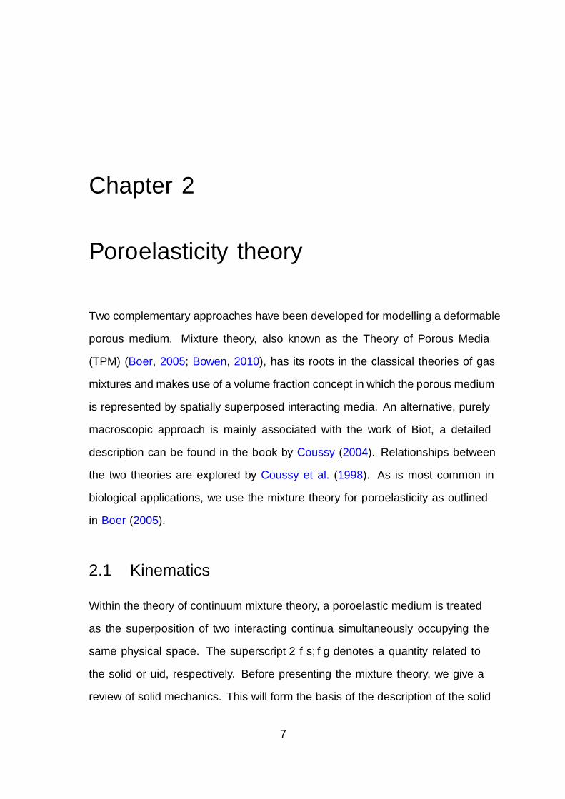
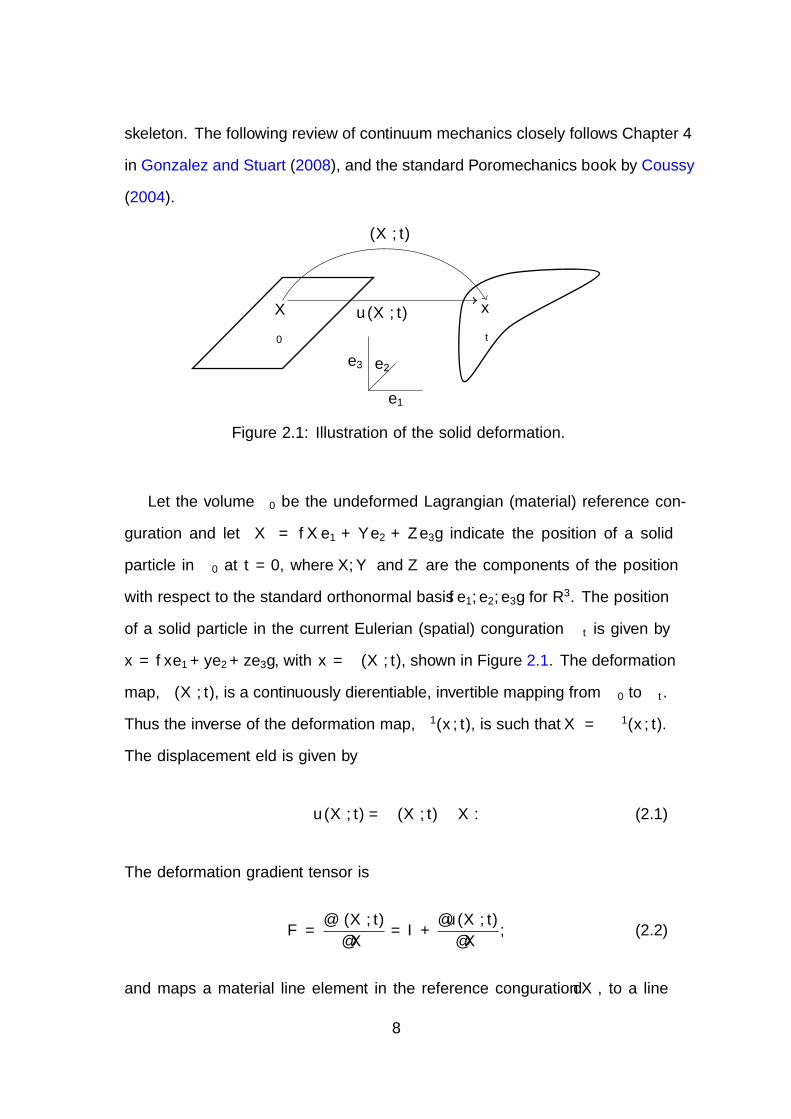
Figure 2.1: Illustration of the solid deformation.

Let the volume Ω0 be the undeformed Lagrangian (material) reference con-

figuration and let X = Xe1 + Y e2 + Ze3 indicate the position of a solid

particle in Ω0 at t = 0, where X, Y and Z are the components of the position

with respect to the standard orthonormal basis e1, e2, e3 for R3. The position

of a solid particle in the current Eulerian (spatial) configuration Ωt is given by

x = xe1 +ye2 +ze3, with x = χ(X, t), shown in Figure 2.1. The deformation

map, χ(X, t), is a continuously differentiable, invertible mapping from Ω0 to Ωt.

Thus the inverse of the deformation map, χ−1(x, t), is such that X = χ−1(x, t).

The displacement field is given by

u(X, t) = χ(X, t)−X. (2.1)

The deformation gradient tensor is

F =∂χ(X, t)

∂X= I +

∂u(X, t)

∂X, (2.2)

and maps a material line element in the reference configuration dX, to a line

8

element dx in the current configuration, i.e. dx = F dX. The symmetric right

Cauchy-Green deformation tensor is given by

C = F TF . (2.3)

The Jacobian is defined as

J = det(F ), (2.4)

and represents the change in an infinitesimal small volume from the reference

to the current configuration. Also note that J > 0, to avoid self penetration of

the body. We also have that J represents the change in an infinitesimal small

volume from a reference volume element dΩ0 to a currret configuration volume

element dΩt

dΩt = JdΩ0. (2.5)

Also, F is invertible, and it is easy to see that the inverse of the deformation

gradient is the deformation gradient of the inverse map

F−1 =∂χ−1(x, t)

∂x=∂X

∂x. (2.6)

We denote by V (X, t) the velocity at time t of the material (fixed) solid particle

X. By definition we have

V (X, t) =∂

∂tχ(X, t). (2.7)

Similarly, we denote by A(X, t) the acceleration of the material solid particle,

given by

A(X, t) =∂2

∂t2χ(X, t). (2.8)

We see that the velocity and acceleration of material particles are material fields.

9

Also note that ∂∂tu(X, t) = ∂

∂tχ(X, t). We will also require a spatial description

of these fields. We denote by vs(x, t) the spatial description of the material solid

velocity field, such that

vs(x, t) =

[∂

∂tχ(X, t)

]∣∣∣∣X=χ−1(x,t)

. (2.9)

Due to the definition of vs in (2.9) we also have (see section 4.4.4 in Gonzalez

and Stuart (2008))

vs(x, t)|x=χ(X,t) =∂

∂tχ(X, t). (2.10)

To simplify the notation we will follow Ateshian et al. (2010) and write

vs(x, t) =∂

∂tχ(X, t). (2.11)

Similarly, for the spatial description of the solid acceleration, we have

as(x, t) =

[∂2

∂t2χ(X, t)

]∣∣∣∣X=χ−1(x,t)

. (2.12)

Notice that vs(x, t) and as(x, t) correspond to the velocity and acceleration

of the solid material particle whose current coordinates are x at time t. The

acceleration of the fluid is given by (see section 3.1 in Boer (2005)),

af =dfvf

dt=

∂

∂tvf + (∇vf )vf . (2.13)

The particle derivative of a field G(x, t) with respect to the particle α (s or

f) is given by

dα

dtG =

∂G∂t

+ (∇G)vα, (2.14)

where ∇(·) = ∂/∂x(·) denotes the partial derivative with respect to the deformed

configuration. We will use ∇ to denote the spatial gradient in Ω(t) rather than

10

the more explicit ∇x=χ(X,t). The latter more clearly indicates the dependency

of the gradient operator on the deformation χ(X, t) and highlights the inherent

nonlinearity that arises due to the fact that the deformation χ(X, t) is one of the

unknowns. Similarly the deformed domain Ωt, is a function of the deformation

map χ, and therefore incorporates another important nonlinearity.

The particle derivative of a material volume with respect to the α-

constituent is given by (see section 1.3.1 in Coussy (2004))

dα

dt

∫Ωt

dΩt =

∫Ωt

∇ · vαdΩt. (2.15)

The particle derivative also applies to a volume integral. Thus, for any quantity

G, associated with the α constituent, we have

dα

dt

∫Ωt

GdΩt =

∫Ωt

(dαGdt

+ G∇ · vα)dΩt =

∫Ωt

(∂G∂t

+∇ · Gvα)dΩt. (2.16)

This is commonly known as the Reynolds transport theorem. In the last step of

(2.16) we have used the identity ∇ · (ψs) = s · ∇ψ + ψ∇ · s for some scalar ψ

and vector s.

2.2 Volume fractions

We restrict our attention to saturated porous media which are assumed to consist

of solid and fluid parts. The fluid accounts for volume fractions φ0(X, t = 0)

and φ(x, t) of the total volume in the reference and the current and deformed

configurations respectively, where φ is known as the porosity. The fractions

for the solid are therefore 1 − φ0 and 1 − φ in the reference and the current

configuration respectively. For a mixture the density in the current configuration

11

is given by

ρ = ρs(1− φ) + ρfφ in Ωt, (2.17)

where ρs and ρf are the densities of the fluid and solid, respectively. We assume

that both the solid and the fluid are incompressible so that ρs = ρs0 and ρf = ρf0 .

For notational convenience we also define

ρs = ρs(1− φ), (2.18)

and

ρf = ρfφ. (2.19)

Due to mass conservation and the incompressibility of both the solid and the

fluid phase we have

J =1− φ0

1− φ , (2.20)

where J represents the change in volume of the solid skeleton. The solid skeleton

includes the solid (tissue in biological applications) and the voids occupied by

the fluid. Note that although the solid is assumed to be incompressible the solid

skeleton is able to change in volume, since fluid can enter or leave the solid

skeleton.

2.3 Conservation of mass

When no mass change occurs, neither for the solid skeleton or the fluid con-

tained in Ωt, using the Reynolds transport theorem (2.16), the balance of mass,

for a volume V (t) that moves with the deforming poroelastic medium, can be

expressed as

ds

dt

∫V (t)

(1− φ)ρsdΩt =

∫V (t)

(∂(1− φ)ρs

∂t+∇ · ((1− φ)ρsvs)

)dΩt,

12

df

dt

∫V (t)

φρfdΩt =

∫V (t)

(∂φρf

∂t+∇ · (φρfvf )

)dΩt.

Thus, the balance of mass for the solid is given by

∂(1− φ)ρs

∂t+∇ · ((1− φ)ρsvs) = 0 in Ωt, (2.21)

where vs is the velocity vector of the solid. Similarly, the balance of mass for

the fluid is given by

∂φρf

∂t+∇ · (φρfvf ) = ρfg in Ωt, (2.22)

where vf is the velocity vector of the fluid and g is a general source or sink term.

Noting that ρs and ρf are constants (in space and time), these can be factored

out of equations (2.21) and (2.22). Adding these two equations then provides

the mass balance or continuity equation of the mixture (see section 8.3 in Boer

(2005)),

∇ · ((1− φ)vs) +∇ · (φvf ) = g in Ωt. (2.23)

2.4 Conservation of momentum

The balance law of linear momentum for each individual constituent is given by

dα

dt

∫V (t)

ραvαdΩt =

∫V (t)

∇ · σα + ραf + pα + Θαvα dΩt. (2.24)

Here σα is the Cauchy stress tensor of the α constituent, f is a volume force

acting on the constituents, pα are interaction forces representing frictional in-

teractions between the solid and fluid, defined later in section 6.5.1, and Θαvα

is the variation of momentum due to the α constituent source term (Chapelle

and Moireau, 2014). Note that from (2.21) and (2.22) that we have Θs = 0 and

13

Θf = ρfg. Using the first step of the Reynolds transport theorem (2.16), and

the chain rule, we obtain

∇ · σα + ραf + pα + Θαvα = ραaα + vα(dαρα

dt+ ρα∇ · vα

)in Ωt, (2.25)

where aα are acceleration vectors of the constituents. Since each constituent

exerts an equal and opposite interaction force on the other,

ps + pf = 0. (2.26)

2.5 Constitutive relations

The interaction force is given by (see (Coussy, 2004, eqn. (3.49)))

ps = −pf = −p∇φ+ φ2k−1 · (vf − vs), (2.27)

where k is the (dynamic) permeability tensor. The first term, p∇φ, accounts

for the pressure effect resulting from the variation of the section offered to the

fluid flow, and the second term, φ2k · (vf − vs), describes the viscous resistance

opposed by the shear stress to the fluid flow from the drag at the internal walls

of the porous network (Coussy, 2004). This particular choice for the interaction

force means that the momentum balance for the fluid flow can later be reduced

to the well known Darcy law.

The permeability tensor in the current configuration is given by

k = J−1Fk0(χ)F T , (2.28)

where k0(χ) is the permeability in the reference configuration, which may be

chosen to be some (nonlinear) function dependent on the deformation. Examples

14

of deformation dependent permeability tensors for biological tissues can be found

in Holmes and Mow (1990); Kowalczyk and Kleiber (1994); Lai and Mow (1980).

The solid stress tensor is given by the effective stress principle (see eqn. (8.62)

in Boer (2005)),

σs = σse − (1− φ)Ip, (2.29)

where σse is the effective stress tensor given by

σse =1

JF · 2∂W (χ)

∂C· F T . (2.30)

Here W (χ) denotes a strain-energy law (hyperelastic Helmholtz energy func-

tional) dependent on the deformation of the solid. The fluid stress tensor can be

written as (see (Boer, 2005, eqn. (8.63)))

σf = σfvis − φIp, (2.31)

where σfvis denotes the viscous stress tensor of the fluid, given by (see Boer (2005,

eqn. (6.145)))

σfvis = µfφ(∇vf + (∇vf )T −2

3∇ · vf ), (2.32)

where µf is the dynamic viscosity of the fluid.

Summing the conservation laws (2.25) for its constituents and applying the

constitutive relations, the conservation of linear momentum for the mixture is

ρsas + ρfaf + vs(dsρs

dt+ ρs∇ · vs

)+ vf

(df ρf

dt+ ρf∇ · vf

)= ∇ · (σe + σvis − pI) + ρf + gvf in Ωt. (2.33)

15

Applying (2.21) and (2.22), along with applications of (2.14), we get

ρsas + ρfaf = ∇ · (σe + σvis − pI) + ρf in Ωt. (2.34)

The momentum equation for the fluid flow can be identified from (2.25) with

α = f as

ρfaf = ∇ · (σfvis − φpI) + ρff + p∇φ− φ2k−1(vf − vs) in Ωt. (2.35)

2.6 Summary of the general poroelasticity model

We consider Ωt to be a bounded domain in R2 or R3, and for the purpose of defin-

ing boundary conditions, ∂Ωt = ΓD ∪ ΓN for displacement and stress boundary

conditions and ∂Ωt = ΓP ∪ ΓF for pressure and flux boundary conditions, with

outward pointing unit normal n. The strong problem for the full mixture theory

model is to find χ(X, t), vf (x, t) and p(x, t) such that

ρsas + ρfaf = ∇ · (σe + σvis − pI) + ρf in Ωt, (2.36a)

ρfaf = ∇ · (σfvis − φpI) + p∇φ− φk−1(vf − vs) + ρff in Ωt, (2.36b)

∇ · ((1− φ)vs) +∇ · (φvf ) = g in Ωt, (2.36c)

χ(X, t)|X=χ−1(x,t) = X + uD on ΓD, (2.36d)

(σe + σvis − pI)n = tN on ΓN , (2.36e)

vf = vfD on ΓF , (2.36f)

(σvis − φpI)n = sP on ΓP , (2.36g)

χ(0) = X, vs(0) = vs0, vf (0) = vf0 in Ω0. (2.36h)

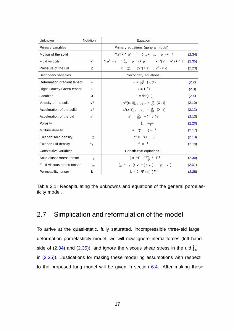
We have also summarised all the variables and corresponding equations in Table

2.1.

16

Unknown Notation Equation

Primary variables Primary equations (general model)

Motion of the solid χ ρsas + ρfaf = ∇ · (σe + σvis − pI) + ρf (2.34)

Fluid velocity vf ρfaf = ∇ · (σfvis − φpI) + p∇φ− φk−1(vf − vs) + ρff (2.35)

Pressure of the fluid p ∇ · ((1− φ)vs) +∇ · (φvf ) = g (2.23)

Secondary variables Secondary equations

Deformation gradient tensor F F = ∂∂Xχ(X, t) (2.2)

Right Cauchy-Green tensor C C = F TF (2.3)

Jacobian J J = det(F ) (2.4)

Velocity of the solid vs vs(x, t)|x=χ(X,t) = ∂∂tχ(X, t) (2.10)

Acceleration of the solid as as(x, t)|x=χ(X,t) = ∂2

∂t2χ(X, t) (2.12)

Acceleration of the fluid af af = ∂∂tvf + (∇vf )vf (2.13)

Porosity φ φ = 1− 1−φ0

J(2.20)

Mixture density ρ ρ = ρs(1− φ) + ρfφ (2.17)

Eulerian solid density ρs ρs = ρs(1− φ) (2.18)

Eulerian fluid density ρf ρf = ρfφ (2.19)

Constitutive variables Constitutive equations

Solid elastic stress tensor σe σse = 1JF · 2∂W (χ)

∂C· F T (2.30)

Fluid viscous stress tensor σvis σfvis = µfφ(∇vf + (∇vf )T − 23∇ · vf ) (2.31)

Permeability tensor k k = J−1Fk0(χ)F T (2.28)

Table 2.1: Recapitulating the unknowns and equations of the general poroelas-ticity model.

2.7 Simplification and reformulation of the model

To arrive at the quasi-static, fully saturated, incompressible three-field large

deformation poroelasticity model, we will now ignore inertia forces (left hand

side of (2.34) and (2.35)), and ignore the viscous shear stress in the fluid (σfvis

in (2.35)). Justifications for making these modelling assumptions with respect

to the proposed lung model will be given in section 6.4. After making these

17

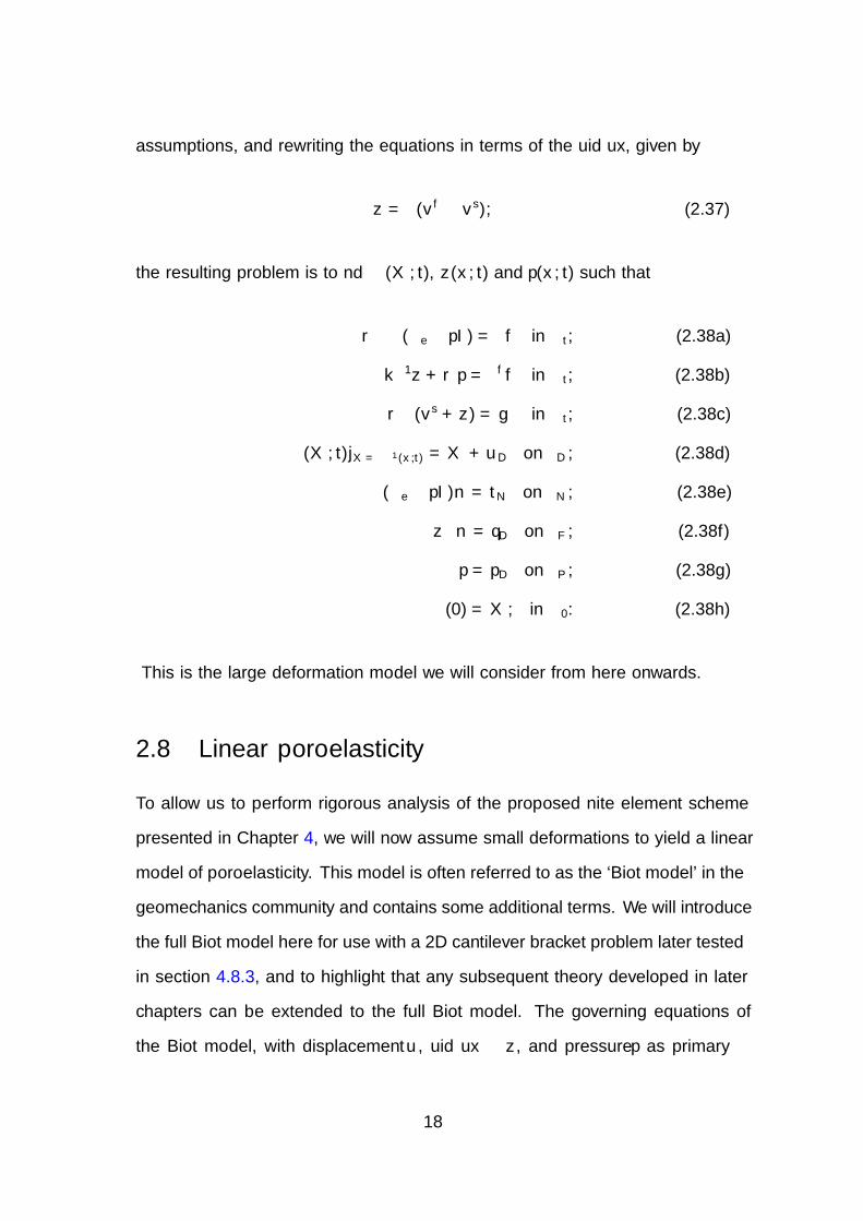
assumptions, and rewriting the equations in terms of the fluid flux, given by

z = φ(vf − vs), (2.37)

the resulting problem is to find χ(X, t), z(x, t) and p(x, t) such that

−∇ · (σe − pI) = ρf in Ωt, (2.38a)

k−1z +∇p = ρff in Ωt, (2.38b)

∇ · (vs + z) = g in Ωt, (2.38c)

χ(X, t)|X=χ−1(x,t) = X + uD on ΓD, (2.38d)

(σe − pI)n = tN on ΓN , (2.38e)

z · n = qD on ΓF , (2.38f)

p = pD on ΓP , (2.38g)

χ(0) = X, in Ω0. (2.38h)

This is the large deformation model we will consider from here onwards.

2.8 Linear poroelasticity

To allow us to perform rigorous analysis of the proposed finite element scheme

presented in Chapter 4, we will now assume small deformations to yield a linear

model of poroelasticity. This model is often referred to as the ‘Biot model’ in the

geomechanics community and contains some additional terms. We will introduce

the full Biot model here for use with a 2D cantilever bracket problem later tested

in section 4.8.3, and to highlight that any subsequent theory developed in later

chapters can be extended to the full Biot model. The governing equations of

the Biot model, with displacement u, fluid flux z, and pressure p as primary

18

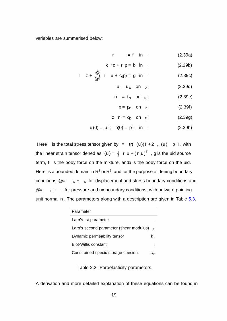
variables are summarised below:

−∇ · σ = f in Ω, (2.39a)

k−1z +∇p = b in Ω, (2.39b)

∇ · z +∂

∂t(α∇ · u+ c0p) = g in Ω, (2.39c)

u = uD on ΓD, (2.39d)

σn = tN on ΓN , (2.39e)

p = pD on ΓP , (2.39f)

z · n = qD on ΓF , (2.39g)

u(0) = u0, p(0) = p0, in Ω. (2.39h)

Here σ is the total stress tensor given by σ = λtr(ε(u))I+ 2µsε(u)−αpI, with

the linear strain tensor defined as ε(u) = 12

(∇u+ (∇u)T

), g is the fluid source

term, f is the body force on the mixture, and b is the body force on the fluid.

Here Ω is a bounded domain in R2 or R3, and for the purpose of defining boundary

conditions, ∂Ω = ΓD + ΓN for displacement and stress boundary conditions and

∂Ω = ΓP + ΓF for pressure and flux boundary conditions, with outward pointing

unit normal n. The parameters along with a description are given in Table 5.3.

Parameter

Lame’s first parameter λ,

Lame’s second parameter (shear modulus) µs,

Dynamic permeability tensor k,

Biot-Willis constant α,

Constrained specific storage coefficient c0.

Table 2.2: Poroelasticity parameters.

A derivation and more detailed explanation of these equations can be found in

19

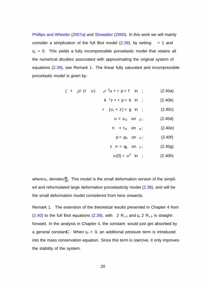
Phillips and Wheeler (2007a) and Showalter (2000). In this work we will mainly

consider a simplification of the full Biot model (2.39), by setting α = 1 and

c0 = 0. This yields a fully incompressible poroelastic model that retains all

the numerical difficulties associated with approximating the original system of

equations (2.39), see Remark 1. The linear fully saturated and incompressible

poroelastic model is given by:

−(λ+ µs)∇(∇ · u)− µs∇2u+∇p = f in Ω, (2.40a)

k−1z +∇p = b in Ω, (2.40b)

∇ · (ut + z) = g in Ω, (2.40c)

u = uD on ΓD, (2.40d)

σn = tN on ΓN , (2.40e)

p = pD on ΓP , (2.40f)

z · n = qD on ΓF , (2.40g)

u(0) = u0 in Ω, (2.40h)

where ut denotes ∂u∂t

. This model is the small deformation version of the simpli-

fied and reformulated large deformation poroelasticity model (2.38), and will be

the small deformation model considered from here onwards.

Remark 1. The extension of the theoretical results presented in Chapter 4 from

(2.40) to the full Biot equations (2.39), with α ∈ R>0 and c0 ∈ R>0 is straight-

forward. In the analysis in Chapter 4, the constant α would just get absorbed by

a general constant C. When c0 > 0, an additional pressure term is introduced

into the mass conservation equation. Since this term is coercive, it only improves

the stability of the system.

20

Chapter 3

Finite element method

3.1 Introduction

A large proportion of the mathematical models in science and engineering take

the form of differential equations. Only in the simplest cases, or under strong

assumptions, is it possible to find exact analytical solutions to the equations

in the model. Numerical methods are an established means of solving differ-

ential equations that are of practical interest in a variety of applied problems.

Finite difference, finite volume and finite element methods are the most widely

used types of such methods. Their basic idea is replacing the infinite-dimensional

problem by a finite-dimensional approximation, which is, generally speaking, eas-

ier to compute. Finite element methods are based on weakening the restrictions

on the solution space in the continuous setting, and searching for the approxi-

mate solution in the subspace which spans basis functions supported on small

regions inside the domain. These methods are well-suited to solving problems

on complex domains, and are therefore widely used in practical applications. In

this work we consider only finite element methods (FEMs) for solving partial

differential equations. This chapter comprises an overview of several theoreti-

cal and practical aspects of classical FEMs. The theory and notation presented

21

here are essential in developing the techniques that form the core of this thesis.

Most of the work presented in this chapter is based on work already presented

in Arthurs (2012); Asner (2013); Bernabeu (2011); Brenner and Scott (2008);

Brezzi and Fortin (1991a). We conclude this chapter by discussing numerical

methods currently available to solve the poroelastic equations.

3.2 Norms and spaces

Let Ω be a bounded domain in R2 or R3, and ∂Ω be the associated boundary.

The space of square integrable functions is then given by

L2(Ω) =

u :

∫Ω

|u(x)|2dx <∞,

with norm

||u||0,Ω =

∫Ω

|u(x)|2dx

1/2

.

This space is equipped with the inner product

(u, v) =

∫Ω

u(x)v(x)dx,

such that ||u||0,Ω = (u, v)1/2. Throughout this thesis we shall frequently refer to

the Sobolev spaces H1(Ω) and H2(Ω). The definitions of these are as follows:

H1(Ω) =

u ∈ L2(Ω) :

∂u

∂xj∈ L2(Ω), j = 1, . . . , n,

,

H2(Ω) =

u ∈ L2(Ω) :

∂u

∂xj∈ L2(Ω), j = 1, . . . , n,

∂2u

∂xi∂xj∈ L2(Ω), i, j = 1, . . . , n

.

22

The corresponding norms are defined as

||u||1,Ω =

||u||20,Ω +

n∑j=1

∣∣∣∣∣∣∣∣ ∂u∂xj∣∣∣∣∣∣∣∣

0,Ω

1/2

,

||u||2,Ω =

||u||20,Ω +

n∑j=1

∣∣∣∣∣∣∣∣ ∂u∂xj∣∣∣∣∣∣∣∣

0,Ω

+n∑

i,j=1

∣∣∣∣∣∣∣∣ ∂2u

∂xi∂xj

∣∣∣∣∣∣∣∣0,Ω

1/2

.

We also define the divergence space

Hdiv(Ω) =v ∈ L2(Ω) : ∇ · v ∈ L2(Ω)

.

The set of functions of L2(∂Ω) which are traces of functions of H1(Ω) onto the

boundary, constitutes a subspace of L2(∂Ω) denoted by H1/2(∂Ω). We will also

briefly use linear and bounded functionals (dual spaces) of H1, H1/2 and Hdiv,

which will be denoted by H−1, H−1/2 and H−1div, respectively.

We define the following norms for continuous in time functions u such that

the norm L2(0, T ;X) satisfies

||u||L2(X) =

(∫ T

0

||u(·, s)||2X ds

)1/2

,

and the norm L∞(0, T ;X) satisfies

||u||L∞(X) = sup ||u(·, s)||X : s ∈ [0, T ] ,

where X is any given function space over Ω. We partition [0, T ] into N evenly

spaced non-overlapping regions (tn−1, tn], n = 1, 2, . . . , N . For any sufficiently

smooth function u(t, x) we define un(x) = u(tn, x). Let the discrete approxima-

tion for all time to be the piecewise constant in time functions v(x, t) = vn(x)

for t ∈ (tn−1, tn]. For such piecewise constant in time functions, v, we define the

23

norms

||v||L2(X) =

(N∑n=1

∆t||vn||2X

)1/2

,

and

||v||L∞(X) = max ||vn||X , n = 1, 2, ..., N .

3.3 Model problem

It is instructive to begin at a simple level and proceed by incrementally adding

to the complexity of the equations we are discretising when explaining the use of

the FEM, so we begin by considering the classical heat equation: given T > 0,

for t ∈ [0, T ] find u(x, t) such that

∂u

∂t−∇ · ∇u = 0 in Ω, (3.1a)

n · ∇u = gN on ΓN , (3.1b)

u = gD on ΓD, (3.1c)

u(x, 0) = u0(x) in Ω. (3.1d)

Here Ω is a bounded domain in R2 or R3, with boundary ∂Ω = ΓN ∪ ΓD, that

has an outward pointing unit normal n. The initial condition is given by u0(x).

In the case where gN = 0, system (3.1) can describe the evolution of heat in an

object with geometry described by Ω, where we have perfect thermal insulation

on ΓN and fixed temperature distributions given by the function gD defined

on the boundary due to some part of the environment with fixed temperature

contacting the object along ΓD.

24

3.3.1 Weak formulation

The strong form of (3.1) requires u to be at least twice differentiable. To weaken

the regularity restrictions we multiply equation (3.1a) by an arbitrary function

v, called a test function, and integrate over Ω:

(∂u

∂t, v

)− (∇ · ∇u, v) = 0.

Applying the divergence theorem, this equation can be rewritten as

(∂u

∂t, v

)− (∇u · n, v)∂Ω + (∇u,∇v)

=

(∂u

∂t, v

)− (∇u · n, v)ΓD − (gN , v)ΓN + (∇u,∇v) = 0.

Here (·, ·)ΓNand (·, ·)ΓD

denote the inner product taken over ΓN and ΓD, respec-

tively. Taking note of the Dirichlet condition (3.1c), and letting v = 0 on ΓD, we

arrive at the following equation:

(∂u

∂t, v

)+ (∇u,∇v) = (gN , v)ΓN .

Note that in this equation the second derivatives of u need not exist. With

that in mind, both the solution and the test functions can come from the space

H1(Ω), as long as they satisfy the appropriate Dirichlet boundary conditions.

For convenience we will use the notation XD = v ∈ H1(Ω)|v = uD on ΓD and

X0 = v ∈ H1(Ω)|v = 0 on ΓD. The weak formulation of (3.1a) is as follows:

Find u ∈ XD such that

(∂u

∂t, v

)+ (∇u,∇v) = (gN , v)ΓN ∀v ∈ X0. (3.2)

25

3.3.2 Time discretisation

We also need to choose a method of treating the time derivative. In this work,

we do so using backward Euler difference quotients, and so we make the approx-

imation ut(x, t+ ∆t) ≈ u(x,t+∆t)−u(x,t)∆t

for some constant time step ∆t. We write

u(x)n for the the temporally-semidiscrete approximation to u(x, n∆t), and our

numerical scheme will yield approximations at times t = 0,∆t, 2∆t, ..., T . In-

serting this difference quotient and assuming that ∆T divides T , equation (3.3)

becomes: for n = 1, 2, ..., T∆t

, find un ∈ XD such that

(un, v) + ∆t (∇un,∇v) = (gN , v)ΓN +(un−1, v

)∀v ∈ X0. (3.3)

3.3.3 Spatial finite element discretisation

In order to solve this problem numerically, we must make it finite dimensional

by discretising it suitably. The finite element approximation space is constructed

as follows: first, the problem domain is partitioned into small element domains,

and second, the element is defined by prescribing for each element domain a set

of nodes and nodal values, and defining suitable basis functions on these, for

example, as piecewise-linear basis functions.

Element domains are normally shaped as triangles or squares in R2, tetra-

hedra or hexahedra in R3. All the nodes, edges and faces of element domains

constitute the problem mesh. Defining a set of local basis functions completes the

finite element space. For a rigorous definition of finite elements, and a description

of different types of elements we refer to Brenner and Scott (2008).

Let T h be a partition of Ω into non-overlapping elements K. We denote by h

the size of the largest element in T h. On the given partition T h we then define

26

the following finite element spaces, to solve the model problem:

XhD =u ∈ C0(Ω) : u|K ∈ P1(K);u = uD on ΓD;∀K ∈ T h

,

Xh0 =u ∈ C0(Ω) : u|K ∈ P1(K);u = 0 on ΓD; ∀K ∈ T h

,

where P1(K) is the space of linear polynomials on K, and C0(Ω) is the space

of continuous functions on Ω. The discretised problem, for each time step, is to

find unh ∈ XhD, for n = 1, 2, ..., T∆t

such that

(unh, vh) + ∆t (∇unh,∇vh) = (gN , vh)ΓN +(un−1h , vh

)∀vh ∈ Xh0. (3.4)

We now choose the Lagrangian basis φ1, φ2, ..., φm of Xh defined by the nodal

values at the nodes x1,x2, ...,xm, namely

φi(xj) = δi,j =

1, i = j

0, i 6= j,

We observe that a basis of Xh0 can be constructed by removing φi with xi ∈ ΓD

from the basis of Xh. Let us assume that the indices of such basis functions

are 1, ...,m, and therefore Xh0 = span φ1, ..., φm. The finite-dimensional weak

problem (3.4) is equivalent to: Find unh ∈ XhD such that

(unh, φi) + ∆t (∇unh,∇φi) = (gN , φi)ΓN +(un−1h , φi

)∀i = 1, ...,m. (3.5)

Any function from Xh can be presented in the form of a basis expansion. Let

this basis expansion for unh be

unh(x) =m∑i=1

uni φi(x),

27

with uni = unh(xi). We define the vector of nodal values to be un = [un1 , ..., unm]T .

Substituting this expression into (3.5), we finally obtain a linear system which

we can solve for un:

(M + ∆tA)un = Mun−1 + g, (3.6)

where we have defined the following matrices and vectors:

A = [aij], aij =

∫Ω

∇φi · ∇φj dx,

M = [mij], mij =

∫Ω

φi · φj dx,

g = [gi], gi =

∫ΓN

gN · φi ds,

The linear system of equations (3.6) can be solved using standard methods such

as Gaussian elimination.

3.4 Mixed methods

Before considering the discretisation of the poroelasticity equations in Chapter 4

we first consider the problems of Darcy and Stokes flow. This is because many of

the difficulties in solving the three-field poroelasticity problem are present when

coupling the Stokes equations (elasticity of the porous mixture) with the Darcy

equations (fluid flow through pores), with a modified incompressibility constraint

that combines the divergence of the displacement velocity and the fluid flux. We

begin with a general formulation of both the Darcy and Stokes flow equations:

A(u) +∇p = f in Ω, (3.7a)

∇ · u = 0 in Ω, (3.7b)

28

where u denotes the velocity vector, p the pressure, f ∈ [L2(Ω)]d, with d = 2, 3,

and A represents the two cases:

• A(u) = k−1u, corresponding to Darcy’s equation.

• A(u) = −2µf∇ · ε(u), corresponding to Stokes equation.

For simplicity we assume Dirichlet conditions on the boundary, that is, u = 0

on ∂Ω for Stokes and u · n = 0 on ∂Ω for Darcy. Mixed methods refer to

the discretisation of different variables using different finite elements. In order

to formulate our finite element method we first need the weak formulation of

problem (3.7). To do this we introduce the spaces

WD = v ∈ Hdiv(Ω) : v · n = 0 on ∂Ω ,

W S =v ∈ [H1(Ω)]d : v = 0 on ΓD

,

and

L20 =

q ∈ L2(Ω) :

∫Γ

q dx = 0

.

We denote the product space WX = WX × L20, where X is chosen to be D for

the Darcy equations or S for the Stokes equations. We also define the following

norm on WX :

||(u, p)||2WX = ||u||2l,Ω + ||∇ · u||20,Ω + ||p||20,Ω,

with l = 0 for Darcy and l = 1 for Stokes. Let a(u,v) be the bilinear form

corresponding to the weak formulation of A(u)

a(u,v) =

(k−1u,v) dx if Darcy’s equation∫Ω

2µ(ε(u) : ε(v)) + λ(∇ · u)(∇ · v) dx if Stokes equation

.

29

Now consider the combined bilinear form

B[(u, p), (v, q)] = a(u,v)− (p,∇ · v) + (q,∇ · u).

The continuous weak formulation of (3.7) is now to find (u, p) ∈ WX such that

B[(u, p), (v, q)] = (f ,v) ∀(v, q) ∈ WX .

For a given finite element subspace WXh ∈ WX , we are left with the finite

dimensional problem: find (uh, ph) ∈ WXh such that:

Bh[(uh, ph), (vh, qh)] = (f ,vh) ∀(vh, qh) ∈ WXh .

To ensure stability and convergence of the discretisation, the discrete subspace

(mixed element) has to be chosen such that the following discrete inf-sup condi-

tion, (Babuska, 1971), is fulfilled:

γ||(uh, ph)||WXh≤ sup

(vh,qh)∈WXh

Bh[(uh, ph), (vh, qh)]

||(v, q)||WXh

∀(u, p) ∈ WXh , (3.8)

where γ > 0 is a constant independent of any mesh parameters. Establishing this

condition ensures wellposedness of the discretisation so that the linear system

arising from the fully discrete method is non-singular and can be solved using

standard methods. It is not trivial to prove (3.8) for different combinations of

finite element. This task has resulted in its own research field within Numerical

Analysis, and countless papers have been published on this topic. In table 3.1

we have documented some popular standard finite element pairs for solving the

Stokes and Darcy equations, and outlined whether these satisfy (3.8), thereby

yielding a stable and optimally converging method, or not. Note that many other

possible discretisations exist.

30

Mixed element Stokes DarcyP1− P1 7 7

P2− P1 3 7

P1− P1 + stab 3 3

P1− P0 7 7

RT − P0 7 3

P1− P0 + stab 3 3

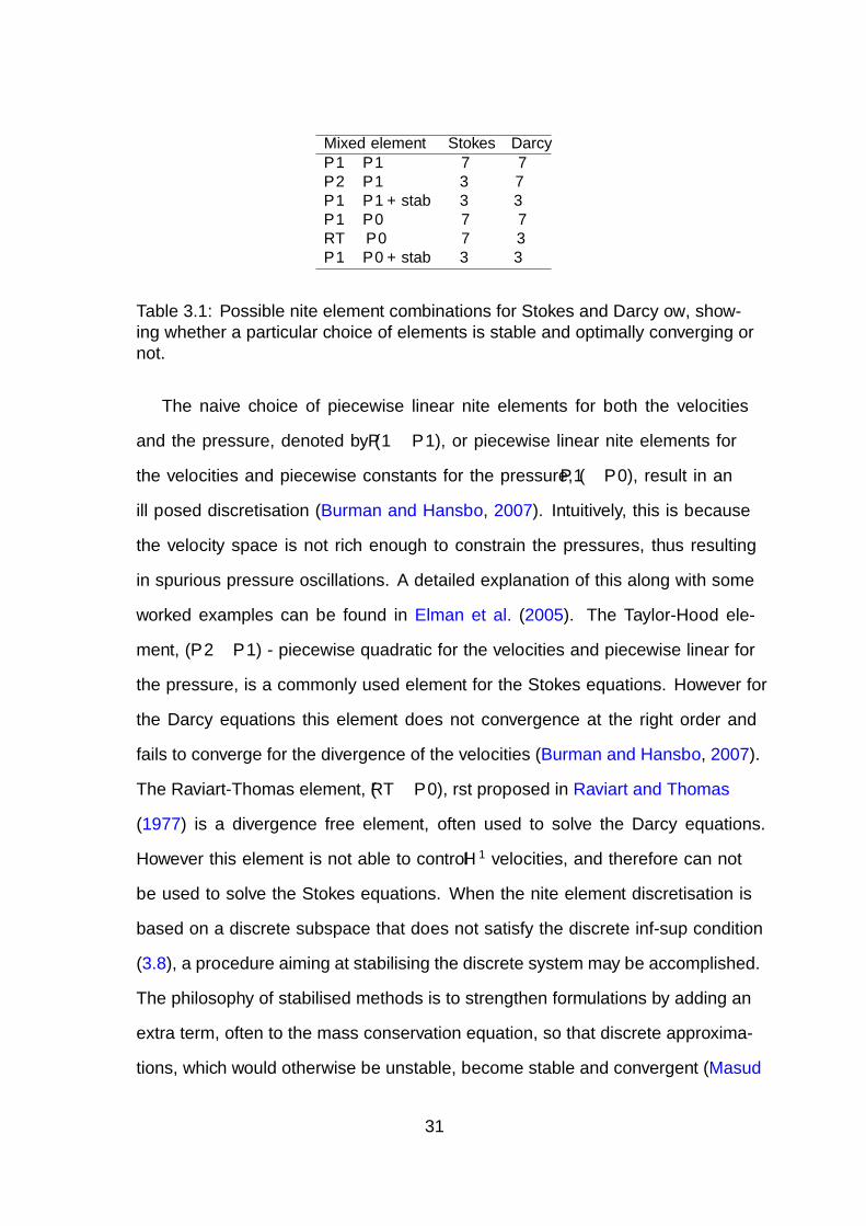
Table 3.1: Possible finite element combinations for Stokes and Darcy flow, show-ing whether a particular choice of elements is stable and optimally converging ornot.

The naive choice of piecewise linear finite elements for both the velocities

and the pressure, denoted by (P1 − P1), or piecewise linear finite elements for

the velocities and piecewise constants for the pressure, (P1 − P0), result in an

ill posed discretisation (Burman and Hansbo, 2007). Intuitively, this is because

the velocity space is not rich enough to constrain the pressures, thus resulting

in spurious pressure oscillations. A detailed explanation of this along with some

worked examples can be found in Elman et al. (2005). The Taylor-Hood ele-

ment, (P2− P1) - piecewise quadratic for the velocities and piecewise linear for

the pressure, is a commonly used element for the Stokes equations. However for

the Darcy equations this element does not convergence at the right order and

fails to converge for the divergence of the velocities (Burman and Hansbo, 2007).

The Raviart-Thomas element, (RT −P0), first proposed in Raviart and Thomas

(1977) is a divergence free element, often used to solve the Darcy equations.

However this element is not able to control H1 velocities, and therefore can not

be used to solve the Stokes equations. When the finite element discretisation is

based on a discrete subspace that does not satisfy the discrete inf-sup condition

(3.8), a procedure aiming at stabilising the discrete system may be accomplished.

The philosophy of stabilised methods is to strengthen formulations by adding an

extra term, often to the mass conservation equation, so that discrete approxima-

tions, which would otherwise be unstable, become stable and convergent (Masud

31

and Hughes, 2002). Numerous stabilisation techniques exist. To stabilise the

equal order piecewise linear pair, a polynomial pressure projection has been pro-

posed in Bochev and Dohrmann (2006) that results in a stable element for both

the Stokes and Darcy equations, (P1−P1 + stab). Also, a pressure jump stabil-

isation, (P1−P0 + stab), that uses a piecewise constant pressure approximation

and is stable and optimally converging for both the Stokes and Darcy equation

has been analysed in Burman and Hansbo (2007). This is the stabilisation we

will modify to solve the poroelastic equations.

3.5 Poroelastic finite element discretisations

3.5.1 Linear discretisations

The linear poroelastic equations are often solved in a reduced displacement and

pressure formulation, from which the fluid flux can then be recovered (Murad and

Loula, 1994; White and Borja, 2008). In Murad and Loula (1994) the stability

and convergence of this reduced displacement pressure (u/p) formulation has

been analysed. They were also able to show error bounds for inf-sup stable

combinations of finite element spaces (e.g. Taylor-Hood elements). In this work

we will keep the fluid flux variable resulting in a three-field, displacement, fluid

flux, and pressure formulation. Keeping the fluid flux as a primary variable has

the following advantages:

i It allows for greater accuracy in the fluid velocity field. This can be of

interest whenever a poroelastic model is coupled with an advection diffusion

equation, e.g. to account for gas exchange, thermal effects, contaminant

transport or the transport of nutrients or drugs within a porous tissue

(Khaled and Vafai, 2003).

ii Physically meaningful boundary conditions can be applied at the interface

32

when modelling the interaction between a fluid and a poroelastic structure

(Badia et al., 2009).

iii It allows for an easy extension of the fluid model from a Darcy to a

Brinkman flow model, for which there are numerous applications in mod-

elling biological tissues (Khaled and Vafai, 2003).

iv It reduces the order of the spatial derivative of the pressure, allowing for

a discontinuous pressure approximation without any additional penalty

terms.

v It avoids the calculation of the fluid flux in post-processing.

Error estimates have been proven in Phillips and Wheeler (2007a,b) for solving

the three-field formulation problem using continuous piecewise linear approxi-

mations for displacements and mixed low-order Raviart Thomas elements for

the fluid flux and pressure variables. However this method was found to be

susceptible to spurious pressure oscillations (Phillips and Wheeler, 2009). To

overcome these pressure oscillations, Li and Li (2012) analysed a discontinuous

three-field method with moderate success, and Yi (2013) analysed a nonconform-

ing three-field method. However no implementation of these methods in 3D has

yet been presented. We hypothesize that this is due to the complexity of these

non-standard elements used, making it very difficult to include them in existing

finite element codes.

In addition to these monolithic approaches there has been considerable work

on operating splitting (iterative) approaches where the poroelastic equations are

separated into a fluid problem and deformation problem (Feng and He, 2010;

Kim et al., 2011; Wheeler and Gai, 2007). Although these methods are often

able to take advantage of existing elasticity and fluid finite element software,

and result in solving a smaller system of equations, these schemes are often only

33

conditionally stable. To ensure that the method is unconditionally stable, mono-

lithic approaches are often preferred. Within this work we will propose a method

that is monolithic and therefore retains the advantage of being unconditionally

stable.

3.5.2 Discretisations valid in large deformations

We will now give a brief overview of different approaches for solving the poroe-

lastic equations valid in large deformations. There has been some work on

operating splitting (iterative) approaches (Chapelle et al., 2010). Again, such

approaches are often only conditionally stable. Some notable quasi-static in-

compressible large deformation monolithic approaches include a mixed-penalty

formulation, and a mixed solid velocity-pressure formulation, both outlined in

Almeida and Spilker (1998), the solid velocity-pressure formulation is similar to

the commonly used reduced (u/p) formulation (Ateshian et al., 2010). These

two-field formulations require a stable mixed element pair such as the popular

Taylor-Hood element to satisfy the LBB inf-sup stability requirement. The key

difficulty, however, that these elements cannot escape is that jumps in material

coefficients may introduce large solution gradients across the interface, requiring

severe mesh refinement. This is because a continuous pressure element is used,

which is unable to reliably capture jumps in the pressure solution (White and

Borja, 2008). In Levenston et al. (1998) a three-field (displacement, fluid flux,

pressure) formulation has been outlined, however this method uses a low-order

mixed finite element approximation without any stabilisation and therefore is not

inf-sup stable. A dynamic three-field finite element using a continuous pressure

approximation has been implemented in Vuong et al. (2015).

34

Chapter 4

A stabilised finite element

method for linear poroelasticity

4.1 Introduction

In this chapter we develop a stabilised, low-order, mixed finite element method

for poroelastic models of biological tissues and restrict our attention to the fully

saturated, incompressible, small deformation case. Our mixed scheme uses the

lowest possible approximation order: piecewise constant approximation for the

pressure and piecewise linear continuous elements for the displacement and fluid

flux.

To ensure stability, a mixed finite element method must satisfy the

Ladyzhenskaya-Babuska-Brezzi (LBB) condition. In this work we use a local

pressure jump stabilisation method pioneered by Burman and Hansbo (2007) for

the study of Stokes and Darcy flows that are coupled via an interface. This ap-

proach provides the natural H1 stability for the displacements and Hdiv stability

for the fluid flux. We also show that the naive approach of using the stabilisation

of the pressure, as is done for the Darcy and Stokes equations in Burman and

Hansbo (2007), results in an approximation that does not converge at an optimal

35

rate. Stabilisation using the time derivative of pressure in the stabilisation term

is shown to be crucial for stability and optimal convergence with refinement and

counterexamples are provided in Section 5.5.

In section 4.2 we formulate the model and its continuous weak formulation

and construct a fully-discrete approximation. In section 4.3 we will introduce

some norms and inequalities. We prove existence and uniqueness of solutions to

this discrete model at each time step in section 4.4, provide an energy estimate

over time in section 4.5, and derive an optimal order a-priori error estimate in

section 4.6. Finally in section 5.5, we present numerical experiments to illustrate

the convergence of the method and its ability to overcome pressure oscillations.

4.2 The poroelastic model

4.2.1 Governing equations

Following Phillips and Wheeler (2007a) and Showalter (2000), we recall the gov-

erning equations (2.40) for a fully saturated, incompressible poroelastic model

−(λ+ µ)∇(∇ · u)− µ∇2u+∇p = f in Ω, (4.1a)

k−1z +∇p = b in Ω, (4.1b)

∇ · (ut + z) = g in Ω, (4.1c)

u = uD on ΓD, (4.1d)

σn = tN on ΓN , (4.1e)

z · n = qD on ΓF , (4.1f)

p = pD on ΓP , (4.1g)

u(·, 0) = u0 in Ω. (4.1h)

36

Remark 4.2.1. Since the above resulting system of equations is linear, for ease of

presentation, we will assume all Dirichlet boundary conditions are homogeneous,

ie., uD = 0, qD = 0, pD = 0.

4.2.2 Weak formulation

We define the following spaces for displacement, fluid flux and pressure respec-

tively,

W E(Ωt) = u ∈ (H1(Ω))d : u = 0 on ΓD,

WD(Ωt) = z ∈ Hdiv(Ω) : z · n = 0 on ΓF,

L(Ωt) =

L2(Ω) if ΓN ∪ ΓP 6= ∅

L20(Ω) if ΓN ∪ ΓP = ∅,

,

where L20(Ω) =

q ∈ L2(Ω) :

∫Ωq dx = 0

, which we combine to construct the

mixed solution space

WX =W E(Ωt)×WD(Ωt)× L(Ωt)

.

We define the bilinear form

a(u,v) =

∫Ω

2µ(ε(u) : ε(v)) + λ(∇ · u)(∇ · v) dx,

for u,v ∈W E(Ωt). This bilinear form is continuous such that

a(u,v) ≤ Cc||u||1,Ω||v||1,Ω ∀u,v ∈ (H1(Ω))d. (4.2)

37

Using Korn’s inequality (Brenner and Scott, 2008; Ciarlet, 1978), and∫Ωλ(∇ · v)(∇ · v) ≥ 0 we have

||v||2a,Ω = a(v,v) ≥ 2µ||ε(v)||20,Ω ≥ Ck||vh||21,Ω ∀v ∈W E(Ωt). (4.3)

Since k is assumed to be a symmetric and strictly positive definite tensor, there

exists eigenfunctions λmin, λmax > 0 such that ∀x ∈ Ω, λmin||η||0,Ω ≤ ηtk(x)η ≤

λmax||η||0,Ω ∀η ∈ Rd, and

λ−1min||w||20,Ω ≥ (k−1w,w) ≥ λ−1

max||w||20,Ω ∀w ∈WD(Ωt). (4.4)

The continuous weak problem is: Find u(x, t) ∈ W E(Ωt), z(x, t) ∈ WD(Ωt),

and p(x, t) ∈ L(Ωt) for any time t ∈ [0, T ] such that:

a(u,v)− (p,∇ · v) = (f ,v) + (tN ,v)ΓN ∀v ∈W E(Ωt), (4.5a)

(k−1z,w)− (p,∇ ·w) = (b,w) ∀w ∈WD(Ωt), (4.5b)

(∇ · ut, q) + (∇ · z, q) = (g, q) ∀q ∈ L(Ωt). (4.5c)

We will assume the following regularity requirements on the data,

f ∈ C1([0, T ]; (H−1(Ω))d),

b ∈ C1([0, T ];H−1div(Ω)),

tN ∈ C1([0, T ];H−1/2(ΓN)),

g ∈ C0([0, T ]; (L2(Ω))d).

(4.6)

For the initial conditions we require that u0 ∈ (H1(Ω))d. The well-posedness

of the continuous two-field formulation has been proven by Showalter (2000).

Lipnikov (2002) proves well-posedness for the continuous three-field formulation

(5.2). In this work we also establish the well-posedness of (5.2) as a result of the

energy estimates proven in section 4.5, see remark 4.5.1.

38

4.2.3 Fully-discrete model

We define the following finite element spaces,

W Eh =

uh ∈ C0(Ω) : uh|K ∈ P1(K) ∀K ∈ T h,uh = 0 on ΓD

,

WDh =

zh ∈ C0(Ω) : zh|K ∈ P1(K) ∀K ∈ T h, zh · n = 0 on ΓF

,

Qh =

ph : ph|K ∈ P0(K) ∀K ∈ T h

if ΓN ∪ ΓP 6= ∅

ph : ph|K ∈ P0(K),∫

Ωph = 0 ∀K ∈ T h

if ΓN ∪ ΓP = ∅

,

where P0(K) and P1(K) are respectively the spaces of constant and linear poly-

nomials on K. We partition [0, T ] into N evenly spaced non-overlapping regions

(tn−1, tn], n = 1, 2, . . . , N , where tn − tn−1 = ∆t. For any sufficiently smooth

function v(t, x) we define vn(x) = v(x, tn) and the discrete time derivative by

vn∆t = vn−vn−1

∆t.

The fully discrete weak problem is: For n = 1, 2, . . . , N , find unh ∈ W Eh ,

znh ∈WDh and pnh ∈ Qh such that

a(unh,vh)− (pnh,∇ · vh) = (fn,vh) + (tN ,vh)ΓN ∀vh ∈W Eh , (4.7a)

(k−1znh ,wh)− (pnh,∇ ·wh) = (bn,wh) ∀wh ∈WDh , (4.7b)

(∇ · un∆t,h, qh) + (∇ · znh , qh) + J(pn∆t,h, qh

)= (gn, qh) ∀qh ∈ Qh. (4.7c)

The stabilisation term is

J(p, q) = δ∑K

∫∂K\∂Ω

h∂K [p][q] ds. (4.8)

Here δ is a stabilisation parameter that is independent of h and ∆t. Here h∂K

denotes the size (diameter) of an element edge in 2D or face in 3D, and [·] is the

jump across an edge or face (taken on the interior edges only). We will see in the

numerical results, section 5.5 that the convergence is not sensitive to δ. The set

39

of all elements is denoted by K, h∂K denotes the size of an element edge in 2D

or face in 3D, and [·] is the jump across an edge. As an example consider [ph],

the jump operator on the piecewise constant pressure. The jump in pressure [ph]

across an element or face E adjoining elements T and S is defined such that

(ph|T − ph|S)nE,T = (ph|S − ph|T )nE,S.

Here nE,T is the outward normal from element T , with respect to edge E, nE,S is

the corresponding inward facing normal, and ph|T and ph|S denote the pressure

in element T and S, respectively.

We also assume

a(u0h,vh) = a(u0,vh) ∀vh ∈W E

h , (4.9a)

J(p0h, qh) = J(p0, qh) ∀qh ∈ Qh, (4.9b)

where p0 ∈ L(Ωt).

4.3 Norms and inequalities

In this section we will introduce some norms and inequalities required for the

remainder of this chapter. Throughout this work, we will let C denote a generic

positive constant, whose value may change from instance to instance, but is

independent of any mesh parameters.

4.3.1 Useful inequalities

Detailed derivations of the following four inequalities can be found in Brenner

and Scott (2008). If f, g ∈ L2(Ω) then by the Cauchy-Schwarz inequality we

40

have ∫Ω

|f(x)g(x)|dx ≤ ||f ||0,Ω||g||0,Ω.

From the triangle inequality we have

||f + g||0,Ω ≤ ||f ||0,Ω + ||g||0,Ω.

For any real numbers a and b, by Young’s inequality,

ab ≤ ε

2a2 +

1

2εb2 ∀ε > 0.

This inequality is sometimes referred to as the arithmetric-geometric mean in-

equality. Next, the Poincare inequality, also known as Poincare-Friedrich’s

inequality says

||v||0,Ω ≤ Cp||∇v||0,Ω ∀v ∈ H1(Ω).

4.3.2 Properties of the J-norm

The stabilisation term gives rise to the semi-norm

|q|J,Ω = J(q, q)1/2.

Using the scaling argument, also used in Burman and Hansbo (2007),

∣∣∣∣h1/2ph∣∣∣∣

0,∂K≤ cz||ph||0,K ∀ph ∈ Qh. (4.10)

Cauchy-Schwarz and the triangle inequality the following bounds for the stabil-

isation term hold.

|ph|J,Ω ≤ C||ph||0,Ω and J(ph, qh, ) ≤ |ph|J,Ω|qh|J,Ω, ∀ph, qh ∈ Qh. (4.11)

41

Furthermore, for any q ∈ H1(Ω),

J(p, q) = 0, ∀p ∈ L(Ωt), (4.12)

see Lemma 1.23 in Di Pietro and Ern (2011).

4.3.3 Approximation results

We now give some approximation results that will be useful later.

Let π1h : H1(Ω) → W E

h and π0h : L2(Ω) → Qh be Clement projections (inter-

polation operators), see Ciarlet (1978).

Lemma 4.3.1. For all v ∈ (H2(Ω))d

and q ∈ H1(Ω) the interpolation operators

satisfy: For s = 0, 1

||v − π1hv||s,Ω ≤ Ch2−s||v||2,Ω, (4.13)∣∣∣∣q − π0hq∣∣∣∣

0,Ω≤ Ch||q||1,Ω, (4.14)

|q − π0hq|J,Ω ≤ Ch||q||1,Ω. (4.15)

Proof. The first two results are standard Brenner and Scott (2008). The final

result is obtained by using the element error estimate provided in Verfurth (1998)

and then summing over all elements.

Due to the surjectivity of the divergence operator, for every p ∈ L2(Ω) there

exists a function vp ∈ (H10 (Ω))d such that∇·vp = −p and ||vp||1,Ω ≤ c||p||0,Ω. This

last inequality can be shown to hold by considering the famous inf-sup condition

related to the continous Stokes problem (Brenner and Scott, 2008; Brezzi and

Fortin, 1991b). We assume that the projection, π1hvp, is stable such that

∣∣∣∣π1hvp∣∣∣∣

1,Ω≤ c||p||0,Ω. (4.16)

42

Furthermore, for any element K ∈ T h

||vp − π1hvp||L2(K) ≤ Ch||vp||H1(ωK), (4.17)

where ωK is a domain made of the elements in T h neighbouring K. For more

details about the properties of this projection we refer to section 4.8 in Brenner

and Scott (2008). This projection will allow us to obtain stability of the pressure

and avoid spurious pressure oscillations. The discrepancy between the projection

and its continuous counterpart will eventually be made up by the stabilisation

term, shown in section 4.4. Combining the above with the trace inequality, see

lemma 3.1 in Verfurth (1998),

∣∣∣∣(vp − π1hvp) · n

∣∣∣∣20,∂K≤ C

∣∣∣∣vp − π1hvp∣∣∣∣

0,K(h−1

∣∣∣∣vp − π1hvp∣∣∣∣

0,K+∣∣∣∣vp − π1

hvp∣∣∣∣

1,K),

(4.18)

we obtain ∣∣∣∣(vp − π1hvp) · n)

∣∣∣∣20,∂K≤ Ch||vp||2H1(ωK). (4.19)

Taking into account ||vp||1,Ω ≤ c||p||0,Ω, we may write

∑K

∫∂K

h−1|(vp − π1hvp) · n|2 ds ≤ ct||p||20,Ω. (4.20)

We also have the following approximation for the time-discretisation error: For

all v ∈ H2(0, T ; (L2(Ω))d)

N∑n=1

∆t

∣∣∣∣∣∣∣∣vn∆t − ∂v

∂t(tn, ·)

∣∣∣∣∣∣∣∣20,Ω

≤ ∆t2∫ T

0

||vtt||20,Ωds. (4.21)

See (Brenner and Scott, 2008; Thomee, 2006) for details.

43

4.3.4 Triple-norms

For all [v, w, q] ∈[(H1(Ω))d ×Hdiv(Ω)× L2(Ω)

]we define the norm

|||[v, w, q]|||2A = ||v||21,Ω + ∆t2||∇ · w||20,Ω + ∆t||w||20,Ω + ||q||20,Ω + |q|2J,Ω. (4.22)

For all [v, w, q] ∈[L∞(0, T ; (H1(Ω))d)× L2(0, T ;Hdiv(Ω))× L2(0, T ;L2(Ω))

]we

define the norm

|||[v, w, q]|||2B = ||v||2L∞(H1) + ||w||2L2(L2) + ||q||2L2(L2). (4.23)

4.4 Existence and uniqueness of solutions to the

fully-discrete model

Well-posedness of the unstabilised fully-discretised system (4.7) (i.e., for δ =

0), with the use of a low order Raviart-Thomas approximation for the fluid

velocity is shown by Phillips and Wheeler (2007b) for c0 > 0, and by Lipnikov

(2002) for c0 ≥ 0. Although as the permeability tends to zero and the porous

mixture becomes impermeable, the three-field linear poroelasticity tends to a

mixed linear elasticity problem (Haga et al., 2012). Hence, in this case this

element becomes unstable, as expected since the elasticity P1−P0 approximation

is known to be unstable. Our method is stable for both the Darcy problem (as

the elasticity coefficients tend to infinity) and the mixed linear elasticity problem

(as the permeability tends to zero), and is therefore stable for all permeabilities

and elasticity coefficients.

Combining the fully discrete equations (4.7a), (4.7b) and (4.7c), after first

multiplying (4.7b) and (4.7c) by ∆t, gives the equivalent problem;

44

For n = 1, 2, . . . , n, find (uh, zh, ph) such that

Bnh [(uh, zh, ph), (vh,wh, qh)]

= (fn,vh) + (tN ,vh)ΓN + ∆t(bn,wh) + ∆t(gn, qh)

+(∇ · un−1h , qh) + J(pn−1

h , qh) ∀(vh,wh, qh) ∈ WXh ,

where

Bnh [(uh, zh, ph), (vh,wh, qh)]

= a(unh,vh) + ∆t(k−1znh ,wh)− (pnh,∇ · vh)−∆t(pnh,∇ ·wh)

+ (∇ · unh, qh) + ∆t(∇ · znh , qh) + J(pnh, qh). (4.24)

The linear form satisfies the following continuity property

|Bnh [(uh, zh, ph), (vh,wh, qh)]| ≤ C |||(unh, znh , pnh)|||A |||(vh,wh, qh)|||A .

We apply Babuska’s theory (Babuska, 1971) to show well-posedness (existence

and uniqueness) of this discretised system at a particular time step. This requires

us to prove a discrete inf-sup type result (Theorem 4.4.1) for the combined bi-

linear form (4.24).

Theorem 4.4.1. Let γ > 0 be a constant independent of any mesh parameters.

Then the finite element formulation (4.7) satisfies the following discrete inf-sup

condition

γ |||(unh, znh , pnh)|||A ≤ sup(vh,wh,qh)∈VXh

Bnh [(uh, zh, ph), (vh,wh, qh)]

|||(vh,wh, qh)|||A∀(uh, zh, ph) ∈ WX

h .

(4.25)

Hence, given a solution at the previous time step the linear system arising from

the fully discrete method for the subsequent time step is non-singular.

45

The following proof follows ideas presented by Burman and Hansbo (2007).

Proof.

Step 1, bounding ||unh||1,Ω, ∆t1/2||znh ||0,Ω, and |pnh|J,Ω.

Choose (vh,wh, qh) = (unh, znh , p

nh), then using (4.3) and (4.4), we obtain,

Bnh [(uh, zh, ph), (uh, zh, ph)] = a(unh,u

nh) + ∆t(k−1znh , z

nh) + J(pnh, p

nh)

≥ Ck||unh||21,Ω + λ−1max∆t||znh ||20,Ω + |pnh|2J,Ω. (4.26)

Step 2, bounding ||pnh||0,Ω.

Choose (vh,wh, qh) = (π1hvpnh , 0, 0) and add 0 = ||pnh||20,Ω + (pnh,∇ · vpnh) to obtain

Bnh [(uh, zh, ph), (π

1hvpnh , 0, 0)] = a(unh, π

1hvpnh) + ||pnh||20,Ω + (pnh,∇ · (vpnh − π

1hvpnh)).

(4.27)

Focusing on the third term in (4.27) only, we apply the divergence theorem and

split the integral over local elements to get

(pnh,∇ · (vpnh − π1hvpnh)) =

∑K

∫∂K

pnh(vpnh − π1hvpnh) · n ds

=∑K

1

2

∫∂K

[pnh](vpnh − π1hvpnh) · n ds.

We thus have

Bnh [(uh, zh, ph), (π

1hvpnh , 0, 0)] = ||pnh||20,Ω + a(unh, π

1hvpnh)

+∑K

1

2

∫∂K

[pnh](vpnh − π1hvpnh) · n ds.

46

Now first applying the Cauchy-Schwarz inequality and (4.2) on the right hand

side to get

Bnh [(uh, zh, ph), (π

1hvpnh , 0, 0)] ≥ ||pnh||20,Ω − Cc||unh||1,Ω

∣∣∣∣π1hvpnh

∣∣∣∣1,Ω

−∑K

1

2

(∫∂K

(h1/2[pnh]

)2ds

)1/2

·(∫

∂K

(h−1/2(vpnh − π

1hvpnh) · n

)2ds

)1/2

.

Now apply Young’s inequality and (4.16) to obtain

Bnh [(uh, zh, ph), (π

1hvpnh , 0, 0)] ≥ ||pnh||20,Ω −

C2c

2ε||unh||21,Ω −

εc

2||pnh||20,Ω

− 1

2εδJ(pnh, p

nh)− ε

2

∑K

∫∂K

h−1|(vpnh − π1hvpnh) · n|2 ds.

Applying (4.20) we obtain

Bnh [(uh, zh, ph), (π

1hvpnh , 0, 0)] ≥ −C

2c

2ε||unh||21,Ω +

(1− (c+ ct)

ε

2

)||pnh||20,Ω

− 1

2εδ|pnh|2J,Ω. (4.28)

Step 3, bounding ∆t||∇ · znh ||0,Ω.

Choosing (vh,wh, qh) = (0, 0,∆t∇ · znh) yields

Bnh [(uh, zh, ph), (0, 0,∆t∇·znh)] = (∇·unh,∆t∇·znh)+∆t2||∇ · znh ||20,Ω+J(pnh,∆t∇·znh).

We bound the first term using the Cauchy-Schwarz inequality followed by Young’s

inequality such that

(∇ · unh,∆t∇ · znh) ≤ Cp2ε||unh||21,Ω +

ε∆t2

2||∇ · znh ||20,Ω.

47

We can also bound the third term as before using the Cauchy-Schwarz inequality

followed by Young’s inequality such that

J(pnh,∆t∇ · znh) ≤ 1

2εJ(pnh, p

nh) +

ε∆t2

2J(∇ · znh ,∇ · znh)

=1

2εJ(pnh, p

nh) + εδ∆t2

∑K

∫∂K

|h1/2∇ · znh |2 ds

≤ 1

2εJ(pnh, p

nh) + εδcz∆t

2||∇ · znh ||20,Ω. (4.29)

Here we have used the scaling argument (4.10) which relates line and surface

integrals and assumes that ∇ · znh is element-wise constant, and (4.11). This

yields

Bnh [(uh, zh, ph), (0, 0,∆t∇ · znh)] ≥ (1− εδcz −

ε

2)∆t2||∇ · znh ||20,Ω

− 1

2ε|pnh|2J,Ω −

Cp2ε||unh||21,Ω. (4.30)

Step 4, Combining steps 1-3.

Finally we can combine (4.26), (4.28) and (4.30) to get control over all the norms

by choosing (vh,wh, qh) = (βunh + π1hvpnh , βz

nh , βp

nh + ∆t∇ · znh), which yields

Bnh [(uh, zh, ph), (βu

nh + π1

hvpnh , βznh , βp

nh + ∆t∇ · znh)] ≥

(βCk −C2c + Cp

2ε)||unh||21,Ω + βλ−1

max∆t||znh ||20,Ω +(

1− εδcz −ε

2

)∆t2||∇ · znh ||20,Ω

+(

1− (c+ ct)ε

2

)||pnh||20,Ω +

(β − 1

2ε− 1

2εδ

)|pnh|2J,Ω, (4.31)

where we can choose

β ≥ max

[C2c + Cp2εCk

+1− CεCk

, λmax(1− Cε

),

1

2ε+

1

2εδ+ 1− Cε

],

48

with C = max[c+ct

2, δcz − 1

2

]. This yields

Bnh [(uh, zh, ph), (βu

nh + π1

hvpnh , βznh , βp

nh +∇ · znh)] ≥ (1− Cε) |||(unh, znh , pnh)|||2A .

To complete the proof, we let (vh,wh, qh) = (βunh + π1hvpnh , βz

nh , βp

nh + ∆t∇ · znh)

and show that for ε sufficiently small there exists a constant C such that

|||(unh, znh , pnh)|||A ≥ C |||(vh,wh, qh)|||A. Using the triangle inequality and (4.16)

we obtain

∣∣∣∣∣∣(βunh + π1hvpnh , βz

nh , βp

nh + ∆t∇ · znh)

∣∣∣∣∣∣2A

≤ C(β2||unh||21,Ω +

∣∣∣∣π1hvpnh

∣∣∣∣21,Ω

+ ∆t2(1 + β)2||∇ · znh ||20,Ω + β2∆t||znh ||20,Ω

+β2||pnh||20,Ω + β2|pnh|2J,Ω + ∆t2|∇ · znh |2J,Ω)

≤ C |||(unh, znh , pnh)|||2A ,

as desired.

4.5 Energy estimate for the fully-discrete model

In this section we construct two new combined bilinear forms, Bn∆t,h (Lem-

mas 4.5.1 and 4.5.2) and Bnh (Lemmas 4.5.3 and 4.5.4). These bilinear forms

are bounded below by Lemmas 4.5.1 and 4.5.3 respectively. Lemma 4.5.2 uses

Lemma 4.5.1 to provide a bound on uh, zh and ph. Lemma 4.5.4 uses Lemma

4.5.3 to provide a bound on ∇ · zh.

49

4.5.1 Bound on the displacement, fluid flux and pressure

Adding (4.7a), (4.7b) and (4.7c), and assuming tN = 0 on Γt, we get the following

Bn∆t,h[(uh, zh, ph), (vh,wh, qh)] = (fn,vh)+(bn,wh)+(gn, qh) ∀(vh,wh, qh) ∈ WX

h ,

(4.32)

where

Bn∆t,h[(uh, zh, ph), (vh,wh, qh)] = a(unh,vh) + (k−1znh ,wh)− (pnh,∇ · vh)

− (pnh,∇ ·wh) + (∇ · un∆t,h, qh) + (∇ · znh , qh) + J(pn∆t,h, qh). (4.33)

Lemma 4.5.1. (uh, zh, ph) satisfies

(N∑n=1

∆tBn∆t,h[(uh, zh, ph), (u

n∆t,h + π1

hvpnh , znh , p

nh)]

+∣∣∣∣u0

h

∣∣∣∣21,Ω

+ |p0h|2J,Ω + ||uh||2L2(H1) + ||ph||2L2(J)

)≥ C

(∣∣∣∣uNh ∣∣∣∣21,Ω + |pNh |2J,Ω + ||zh||2L2(L2) + ||ph||2L2(L2)

).

Proof. For n = 1, 2, . . . , N we choose (vh,wh, qh) = (un∆t,h + π1hvpnh , z

nh , p

nh) in

(4.33), multiplying by ∆t, and summing over all time steps, we get

N∑n=1

∆tBn∆t,h[(uh, zh, ph), (u

n∆t,h + π1

hvpnh , znh , p

nh)]

=N∑n=1

∆ta(unh,un∆t,h) +

N∑n=1

∆tJ(pn∆t,h, pnh) +

N∑n=1

∆tk−1(znh , znh)

+N∑n=1

∆ta(unh, π1hvpnh)−

N∑n=1

∆t(pnh,∇ · π1hvpnh). (4.34)

We now bound each of the above terms on the right hand side of (4.34) individ-

50

ually before combining the results.

N∑n=1

∆ta(unh,un∆t,h) =

N∑n=1

∆t

(1

∆t||unh||2a,Ω −

1

∆ta(unh,u

n−1h )

)≥ Ck

2

∣∣∣∣uNh ∣∣∣∣21,Ω − Cc2

∣∣∣∣u0h

∣∣∣∣21,Ω, (4.35)

where we have used (4.2) and (4.3) in the last step. Using (4.28) we have

N∑n=1

∆ta(unh, π1hvp)−

N∑n=1

∆t(pnh,∇ · π1hvp) ≥ −

Cc2ε||uh||2L2(H1)

+(

1−(c+

ct2

) ε2

)||ph||2L2(L2) −

1

4ε||ph||2L2(J).

Using (4.4),

N∑n=1

∆t(k−1(znh , znh))) ≥ λ−1

max||zh||2L2(L2). (4.36)

The intermediate steps for the next bound have been omitted because they are

very similar to (4.35). Thus

N∑n=1

∆tJ(pn∆t,h, pnh) ≥ 1

2|pNh |2J,Ω −

1

2|p0h|2J,Ω. (4.37)

We can now combine these intermediate results (4.35), (4.5.1), (4.36) and (4.37)

to obtain from (4.34)

N∑n=0

∆tBnδt,h[(uh, zh, ph), (u

n∆t,h + π1

hvp, znh , p

nh)] +

Cc2

∣∣∣∣u0h

∣∣∣∣21,Ω

+Cc2ε||uh||2L2(H1) +

1

4ε||ph||2L2(J) +

1

2|p0h|2J,Ω

≥ Ck2

∣∣∣∣uNh ∣∣∣∣21,Ω +1

2|pNh |2J,Ω + λ−1

max||zh||2L2(L2) + (1− Cε) ||ph||2L2(L2). (4.38)

Finally, choosing ε sufficiently small completes the proof.

51

Lemma 4.5.2. (uh, zh, ph) satisfies

∣∣∣∣uNh ∣∣∣∣21,Ω + |pNh |2J,Ω + ||zh||2L2(L2) + ||ph||2L2(L2) ≤ C(T ).

Proof. For n = 1, 2, . . . , N we choose (vh,wh, qh) = (un∆t,h + π1hvpnh , z

nh , p

nh) in

(4.33), multiplying by ∆t, and summing yields

N∑n=1

∆tBn∆t,h[(u

nh, z

nh , p

nh), (un∆t,h + π1

hvpnh , znh , p

nh)] =

N∑n=1

∆t(fn,un∆t,h + π1hvpnh)

+N∑n=1

∆t(bn, znh) +N∑n=1

∆t(gn, pnh).

Let us note that,

N∑n=1

∆t(fn,un∆t,h) =N∑n=1

(fn,unh − un−1h )

= (fN ,uNh )− (f 1,u0h)−

N−1∑n=1

(fn+1 − fn,unh), (4.39)

and further that

−N−1∑n=1

(fn+1 − fn,unh) ≤ CN−1∑n=1

∣∣∣∣fn+1 − fn∣∣∣∣

0,Ω||unh||0,Ω

≤ C

N−1∑n=1

∫ tn+1

tn

||ft||0,Ω1/2

||unh||1,Ω ≤ C

(1

2ε||ft||2L2(L2) +

ε

2||uh||2L2(L2)

).

Now using the above, Lemma 4.5.1, the Cauchy-Schwarz and Young’s inequali-

ties, choosing ε sufficiently small, and noting (4.16), we arrive at

∣∣∣∣uNh ∣∣∣∣21,Ω+|pNh |2J,Ω+||zh||2L2(L2)+||ph||2L2(L2) ≤ C

(||uh||2L2(H1) + ||ph||2L2(J) +

∣∣∣∣fN ∣∣∣∣20,Ω

+ ||ft||2L2(L2) +∣∣∣∣u0

h

∣∣∣∣20,Ω

+ |p0h|2J,Ω +

∣∣∣∣f 1∣∣∣∣2L2(L2)

+ ||f ||2L2(L2) + ||b||2L2(L2) + ||g||2L2(L2)

).

52

Using Lemma 4.5.2 and regularity to bound the third term and upwards on the

righthand side we obtain

∣∣∣∣uNh ∣∣∣∣21,Ω + |pNh |2J,Ω + ||zh||2L2(L2) + ||ph||2L2(L2) ≤ C(

1 + ||uh||2L2(H1) + ||ph||2L2(J)

).

Upon applying the Gronwall lemma to the above inequality we obtain the desired

result.

4.5.2 Bound on the divergence of the fluid flux

In order to bound the divergence of the fluid flux we now define the bilinear

form Bnh . We first show how we derive Bnh from the fully-discrete weak form

(4.7), for which we know that a solution (uh, zh, ph) exists for test functions

(vh,wh, qh) ∈ VXh . Adding (4.7a) and (4.7b), assuming tN = 0 on Γt, and

summing we have

N∑n=1

a(unh,vh) +N∑n=1

(k−1znh ,wh)−N∑n=1

(pnh,∇ · vh)−N∑n=1

(pnh,∇ ·wh)

=N∑n=1

(fn,vh) +N∑n=1

(bn,wh) ∀(vh,wh, qh) ∈ VXh . (4.40)

For the purposes of this proof we now introduce initial conditions for the fluid

flux and the pressure, z0 ∈ Hdiv(Ω) and p0 ∈ L(Ωt) respectively. We also define

their projections into their respective finite element spaces by z0h := π0

hz0 and

p0h := π0

hp0.

53

Adding (4.7a) and (4.7b), and summing from 0 to N − 1, we have

N∑n=1

a(un−1h ,vh) +

N∑n=1

(k−1zn−1h ,wh)−

N∑n=1

(pn−1h ,∇ · vh)−

N∑n=1

(pn−1h ,∇ ·wh)

=N∑n=1

(fn−1,vh) +N∑n=1

(bn−1,wh) ∀(vh,wh, qh) ∈ VXh . (4.41)

Taking (4.7c), multiplying by ∆t, and summing we have

N∑n=1

∆t(∇ · un∆t,h, qh) +N∑n=1

∆t(∇ · znh , qh) +N∑n=1

∆tJ(pn∆t,h, qh)

=N∑n=1

∆t(gn, qh) ∀(vh,wh, qh) ∈ VXh . (4.42)

Now adding (4.40) and (4.42), and subtracting (4.41) we get

N∑n=1

∆tBnh [(uh, zh, ph), (vh,wh, qh)]

=N∑n=1

∆t(fn∆t,vh) +N∑n=1

∆t(bn∆t,wh) +N∑n=1

∆t(gn, qh) ∀(vh,wh, qh) ∈ VXh ,

where

Bnh [(uh, zh, ph), (vh,wh, qh)] = a(un∆t,h,vh) + (k−1zn∆t,h,wh)

− (pn∆t,h,∇ · vh)− (pn∆t,h,∇ ·wh) + (∇ · un∆t,h, qh) + (∇ · znh , qh) + J(pn∆t,h, qh).

(4.43)

With these preliminaries, we may now bound Bnh from below.

54

Lemma 4.5.3. For all β > β? > 0, (uh, zh, ph) satisfies

N∑n=1

∆t Bnh [(uh, zh, ph), (βun∆t,h + π1

hvp, βznh , βp

n∆t,h +∇ · znh)] +

∣∣∣∣z0h

∣∣∣∣20,Ω≥

C(||u∆t,h||2L2(H1) +

∣∣∣∣zNh ∣∣∣∣20,Ω + ||p∆t,h||2L2(L2) + ||p∆t,h||2L2(J) + ||∇ · zh||2L2(L2)

).

Proof. For n = 1, 2, . . . , N we choose (vh,wh, qh) = (βun∆t,h+π1hvpnh , βz

nh , βp

n∆t,h+

∇ · znh) in (4.43)

N∑n=1

∆tBnh [(uh, zh, ph), (βun∆t,h + π1

hvp, βznh , βp

n∆t,h +∇ · znh)]

=N∑n=1

∆ta(un∆t,h, βun∆t,h) +

N∑n=1

∆tk−1(zn∆t,h, βznh) +

N∑n=1

∆t(∇ · znh ,∇ · znh)

+N∑n=1

∆t(un∆t,h,∇ · znh) +N∑n=1

∆tJ(pn∆t,h,∇ · znh) +N∑n=1

∆tJ(pn∆t,h, βpn∆t,h)

+N∑n=1

∆ta(un∆t,h, π1hvp)−

N∑n=1

∆t(pn∆t,h,∇ · π1hvp). (4.44)

For all ε > 0 using (4.3), (4.4), the Cauchy-Schwarz, Young’s and Poincare

inequalities, (4.11) and (4.10) on ∇·znh , and an approach similar to step 2 in the

proof of Theorem 4.4.1 for the final two terms on the righthand side, we obtain

N∑n=1

∆tBnh [(uh, zh, ph), (βun∆t,h + π1

hvp, βznh , βp

n∆t,h +∇ · znh)]

≥(βCk −

Cp + Cc2ε

)||u∆t,h||2L2(H1) +

βλ−1max

2

∣∣∣∣zNh ∣∣∣∣20,Ω +

(β − 3

4ε

)||p∆t,h||2L2(J)

+ (1− ε(1 + cz)) ||∇ · zh||2L2(L2) −βλ−1

min

2

∣∣∣∣z0h

∣∣∣∣20,Ω

+ (1− Cε) ||p∆t,h||2L2(L2).

(4.45)

Finally choosing ε sufficiently small and β ≥ max[Cp

2Ckε, 3

4ε

]completes the proof.

55

The following Lemma shows the divergence control of the fluid flow.

Lemma 4.5.4. zh obtained from (4.43) satisfies

||∇ · zh||2L2(L2) ≤ C.

Proof. For n = 1, 2, . . . , N we choose (vh,wh, qh) = (βun∆t,h+π1hvpnh , βz

nh , βp

n∆t,h+

∇ · znh) in (4.43) yielding

N∑n=1

∆tBnh [(unh, znh , p

nh), (βun∆t,h + π1

hvpnh , znh , βp

n∆t,h +∇ · znh)]

=N∑n=1

∆t(fn∆t, βun∆t,h + π1

hvpnh) +N∑n=1

∆t(bn∆t, βznh)

+N∑n=1

∆t(gn, βpn∆t,h +∇ · znh).

Using Lemma 4.5.3, the Cauchy-Schwarz and Young’s inequalities, and (4.16),

along with ideas already presented in the proof of Lemma 4.5.2

||u∆t,h||2L2(H1) + ||p∆t,h||2L2(L2) + ||p∆t,h||2L2(J) +∣∣∣∣zNh ∣∣∣∣20,Ω + ||∇ · zh||2L2(L2)

≤ C(||ft||2L2(L2) + ||bt||2L2(L2) + ||ph||2L2(L2) + ||zh||2L2(L2) +||g||2L2(L2)

).

Finally, using Lemma 4.5.2 to bound ||ph||L2(L2), applying a Gronwall lemma, and

using regularity, we obtain the desired result.

56

4.5.3 The energy estimate

Theorem 4.5.5. The solution to the fully-discrete problem (4.7) satisfies the

energy estimate

||uh||2L∞(H1) + ||ph||2L∞(J) + ||zh||2L2(L2) + ||ph||2L2(L2) + ||∇ · zh||2L2(L2) ≤ C.

Proof. The proof follows from combining Lemma 4.5.2 and Lemma 4.5.4, and

noting that these lemmas hold for all time steps n = 0, 1, ..., N . This then gives

the desired discrete in time L∞ bounds.

Remark 4.5.1. Having proven Theorem 4.5.5, it is now a standard calculation to

show that the discrete Galerkin approximation converges weakly, as ∆t, h → 0,

to the continuous problem with respect to continuous versions of the norms of

the energy estimate in Theorem 4.5.5. This in turn shows that the continuous

variational problem is well-posed. Due to the linearity of the variational form

and noting that |v|J,Ω → 0 as h→ 0, these calculations are straight forward and

closely follow the existence and uniqueness proofs presented in Zenısek (1984)

and Barucq et al. (2005) for the linear two-field Biot problem and a nonlinear

Biot problem, respectively.

4.6 A-priori error analysis

Lemma 4.6.1 provides a Galerkin orthogonality result obtained by comparing

continuous and discrete weak forms, which is the corner stone of the error anal-

ysis. Lemma 4.3.1 is a standard approximation result for projections. Lemma

4.6.2 bounds the auxiliary errors for displacement, flux and pressure in the ap-

propriate norms and Lemma 4.6.3 bounds the auxiliary error for the divergence

of the flux. Since Lemmas 4.6.2 and 4.6.3 bound the auxiliary errors at the

57

same order as the projection errors, combining projection and auxiliary errors in

Theorem 4.6.4 provides an optimal error estimate.

We define the finite element error functions

eu = u− uh, ez = z − zh, ep = p− ph.

We introduce the following projection errors:

ηu = u− π1hu, ηz = z − π1

hz, ηp = p− π0hp,

where we have assumed z(·, tn) ∈ (H1(Ω))d. Auxiliary errors:

θnu(·) = π1hu(·, tn)− unh(·), θnz(·) = π1

hz(·, tn)− znh(·), θnp (·) = π0hp(·, tn)− pnh(·),

(4.46)

and time-discretisation errors:

ρnu(·) =u(·, tn)− u(tn−1, ·)

∆t− ∂u(·, tn)

∂t, ρnp =

p(·, tn)− p(·, tn−1)

∆t− ∂p(·, tn)

∂t.

(4.47)

4.6.1 Galerkin orthogonality

We now give a Galerkin orthogonality type argument for analysing the difference

between the fully-discrete approximation and the true solution. For this we

introduce the continuous counterpart of the fully-discrete combined weak form

(4.32) given by

Bn[(u, z, p), (v,w, q)] = (f(·, tn),v) + (b(·, tn),w) + (g(·, tn), q) ∀(v,w, q) ∈ VX ,

58

where

Bn[(u, z, p), (v,w, q)] = a(u(·, tn),v) + k−1(z(·, tn),w)− (p(·, tn),∇ · v)

−(p(·, tn),∇ ·w) + (∇ · ut(·, tn), q) + (∇ · z(·, tn), q).

Lemma 4.6.1. Assuming (u(·, tn), z(·, tn), p(·, tn)) ∈ (H1(Ω))d × Hdiv(Ω) ×

(H1(Ω) ∩ L(Ωt))

Bn∆t,h[(eu, ez, ep), (vh,wh, qh)] = (∇ · ρnu, qh) + J(ρnp , qh) ∀(vh,wh, qh) ∈ VXh .

Proof. Subtracting the discrete weak form (4.32) from the continuous weak form

(4.6.1), we obtain

Bn[(u, z, p), (vh,wh, qh)]−Bn∆t,h[(uh, zh, ph), (vh,wh, qh)] = 0, ∀(vh,wh, qh) ∈ VXh .

Now add J(pt(·, tn), q) = 0 to the left hand side, see (4.12). Finally add (∇ ·

(u∆t(·, tn)− ut(·, tn)) , q)+J(p∆t(·, tn)−pt(·, tn), q) to the left and the righthand

side to obtain the desired result.

4.6.2 Auxiliary error estimates

Lemma 4.6.2.

|||[θu,θz, θp]|||2B + ||θp||2L∞(J) ≤ C(T )(h2 + ∆t2). (4.48)

Proof. Using Lemma 4.6.1 and choosing vnh = θn∆t,u + π1hvpnh , wn

h = θnz , qnh = θnp ,

59

we get

Bn∆t,h[(θ

nu + ηnu,θ

nz + ηnz , θ

np + ηnp ), (θn∆t,u + π1

hvpnh ,θnz , θ

np )]

= (∇ · ρnu, θnp ) + J(ρnp , θnp ).

Rearranging gives

Bn∆t,h[(θ

nu,θ

nz , θ

np ), (θn∆t,u + π1

hvpnh ,θnz , θ

np )]

= (∇ · ρnu, θnp ) + J(ρnp , θnp )−Bn

∆t,h[(ηnu,η

nz , η

np ), (θn∆t,u + π1

hvpnh ,θnz , θ

np )].

Expanding the righthand side, noting that (ηnp ,∇ · (θn∆t,u + π1hvp)) = 0,

(ηnp ,∇ · θnz) = 0, multiplying both sides by ∆t and summing gives

N∑n=1

∆tBn∆t,h[(θ

nu,θ

nz , θ

np ), (θn∆t,u + π1

hvpnh ,θnz , θ

np )] =

7∑i=1

Φi, (4.49)

where

Φ1 = −N∑n=1

∆ta(ηnu,θn∆t,u),

Φ3 = −N∑n=1

∆ta(ηnu, π1hvp),

Φ5 =N∑n=1

∆t(∇ · ρnu, θnp ),

Φ7 = −N∑n=1

∆t(θnp ,∇ · (ηn∆t,u + ηnz)).

Φ2 = −N∑n=1

∆t(k−1(ηnz ,θnz)),

Φ4 = −N∑n=1

∆tJ(ηn∆t,p, θnp ),

Φ6 =N∑n=1

∆tJ(ρnp , θnp ),

We now individually consider the terms on the right hand side of (4.49):

To bound the first quantity, we use (4.21), Lemma 4.3.1, the triangle, Cauchy-

60

Schwarz and Young’s inequalities, θ0u = 0, and (4.2),

Φ1 = −N∑n=1

a(ηnu,θnu − θn−1

u )

= −a(ηNu ,θNu ) +

N∑n=1

a(ηnu − ηn−1u ,θn−1

u )

= −a(ηNu ,θNu ) + ∆t

N∑n=1

a

((I − π1

h

)(ρnu +

∂u(·, tn)

∂t

),θn−1u

)≤ εC

∣∣∣∣θNu ∣∣∣∣21,Ω +Ch2

ε

∣∣∣∣uN ∣∣∣∣22,Ω

+ εC||θu||2L2(H1) +Ch2

2ε||ut||2L2(H2)

+C∆t2

2ε||utt||2L2(H1).

Next, using (4.4), Young’s inequality, (4.16) and Lemma 4.3.1,

Φ2 ≤ε

2||θz||2L2(L2) +

λ−2minh

2

2ε||z||2L2(H1).

Using (4.2), Young’s inequality and Lemma 4.3.1,

Φ3 ≤ε

2

∣∣∣∣π1hvpnh

∣∣∣∣2L2(H1)

+C

2ε||ηu||2L2(H1) ≤

εc2

2||θp||2L2(L2) +

Ch2

2ε||u||2L2(H2).

The bound on Φ4 is obtained using a similar argument to the bound on Φ1,

Φ4 ≤ ε||θp||2L2(J) +h2

2ε||pt||2L2(H1) +

∆t2

2ε||ptt||2L2(H1).

Using the Cauchy-Schwarz and Young’s inequalities and Lemma 4.3.1,

Φ5 ≤ε

2||θp||2L2(L2) +

∆t2

2ε||utt||2L2(L2) and Φ6 ≤

ε

2||θp||2L2(J) +

∆t2

2ε||ptt||2L2(L2).

Finally, using the Cauchy-Schwarz and Young’s inequalities, and a similar argu-

61

ment to the bound on Φ1,

Φ7 ≤3ε

2||θp||2L2(L2) +

h2

2ε||ut||2L2(H2) +

∆t2

2ε||utt||2L2(H1) +

h2

2ε||z||2L2(H2).

Combining these bounds with an application of coercivity Lemma 4.5.1 to (4.49),

noting the assumed regularity of the continuous solution and choosing ε suffi-

ciently small, gives

∣∣∣∣θNu ∣∣∣∣21,Ω+|θNp |2J,Ω+||θz||2L2(L2)+||θp||2L2(L2) ≤ C

(||θu||2L2(H1) + ||θp||2L2(J) + h2 + ∆t2

).

(4.50)

An application of Gronwall’s lemma gives

∣∣∣∣θNu ∣∣∣∣21,Ω + |θNp |2J,Ω + ||θz||2L2(L2) + ||θp||2L2(L2) ≤ C(T )(h2 + ∆t2

).

Because the above holds for all time steps n = 0, 1, ..., N , we can get the desired

L∞ bounds to complete the proof of the theorem.

We now present an a-priori auxiliary error estimate of the fluid flux, in its

natural Hdiv norm.

Lemma 4.6.3. Assuming u ∈ H2(

0, T ; (H1(Ω))d)∩H1

(0, T ; (H2(Ω))

d)

, z ∈

L2(

0, T ; (H2(Ω))d)

and p ∈ H2 (0, T ; J ∩ L(Ωt)) ∩ H1(0, T ;H1(Ω)), then the

finite element solution (4.7) satisfies the auxillary error estimate

||∇ · θz||2L2(L2) ≤ C(T )(h2 + ∆t2). (4.51)

Proof. Similarly to the approach taken in obtaining (4.43) we may easily obtain

the following identity

N∑n=1

∆tBnh [(θnu,θnz , θ

np ), (βθn∆t,u + π1

hvθn∆t,p , βθnz , βθ

n∆t,p +∇ · θnz)] =

6∑i=1

Ψi,

62

where

Ψ1 = −N∑n=1

∆ta(ηn∆t,u, βθn∆t,u + π1

hvθn∆t,p),

Ψ2 = −N∑n=1

∆t(∇ · (ηn∆t,u + ηnz),∇ · θnz + βθn∆t,p),

Ψ3 =N∑n=1

∆tJ(ηn∆t,p, βθn∆t,p +∇ · θnz), Ψ4 = −

N∑n=1

∆t(k−1(ηn∆t,z, βθnz)),

Ψ5 =N∑n=1

∆tJ(ρnp , βθn∆t,p +∇ · θnz), Ψ6 =

N∑n=1

∆t(∇ · ρnu, βθn∆t,p +∇ · θnz).

We now bound the terms on the right hand side of (4.52) using machinery de-

veloped during the previous proof:

Ψ1 ≤Cε

2||θ∆t,u||2L2(H1) +

c2ε

2||θ∆t,p||2L2(L2) +

Ch2

2ε||ut||2L2(H2)

+C

2ε∆t2||utt||2L2(H1), (4.52)

Ψ2 ≤ ε||∇ · θz||2L2(L2) + ε||θ∆t,p||2L2(L2) +Ch2

2ε

(||ut||2L2(H2) + ||z||2L2(H2)

)+C

2ε∆t2||utt||2L2(H1), (4.53)

Ψ3 ≤ εC||∇ · θz||2L2(L2) + ε∣∣∣∣θn∆t,p∣∣∣∣2L2(J)

+Ch2

2ε||pt||2L2(H1) (4.54)

+C

2ε∆t2||ptt||2L2(J), (4.55)

Ψ4 ≤ ε||θz||2L2(L2) +Ch2

2ε||zt||2L2(H1) +

C

2ε∆t2||ztt||2L2(L2), (4.56)

Ψ5 ≤ ε||θ∆t,p||2L2(J) + εC||∇ · θz||2L2(L2) +C∆t2

2ε||ptt||2L2(J), (4.57)

Ψ6 ≤ ε||θ∆t,p||2L2(L2) + ε||∇ · θz||2L2(L2) +C

2ε∆t2||utt||2L2(H1). (4.58)

We can now combine the individual bounds (4.52), (4.53), (4.55), (4.56), (4.57),

and (4.58), with the coercivity result Lemma 4.5.3, choose β sufficiently large,

use the assumption θ0z = 0, the assumed regularity of u, z and p, and choose ε

63

sufficiently small to obtain

∣∣∣∣θNz ∣∣∣∣20,Ω + ||∇ · θz||2L2(L2) ≤ C||θz||2L2(L2) + C(h2 + ∆t2).

Applying Gronwall’s lemma, we get the desired result.

4.6.3 The a-priori error estimate

Combining the previous lemmas we have the following.

Theorem 4.6.4. Assuming u ∈ H2(

0, T ; (L2(Ω))d)∩H1

(0, T ; (H2(Ω))

d)

, z ∈

L2(

0, T ; (H1(Ω))d)

and p ∈ H2 (0, T ;H1(Ω) ∩ L(Ωt)), then the finite element

solution (4.7) satisfies the error estimate

|||eu, ez, ep|||2B ≤ C(h2 + ∆t2).

Assuming u ∈ H2(

0, T ; (H1(Ω))d)∩H1

(0, T ; (H2(Ω))

d)

, z ∈ L2(

0, T ; (H2(Ω))d)

and p ∈ H2 (0, T ; J ∩ L(Ωt)) ∩H1(0, T ;H1(Ω)), then the finite element solution

(4.7) satisfies the error estimate

|||eu, ez, ep|||2B + ||∇ · ez||2L2(L2) ≤ C(h2 + ∆t2).

Proof. We first write the errors as enu = ηnu + θnu, and similarly for the other

variables. Using lemma 4.3.1 we can bound the projection errors, and using

lemma 4.6.2 and lemma 4.6.3 we can bound the auxillary errors to give the

desired result.

64

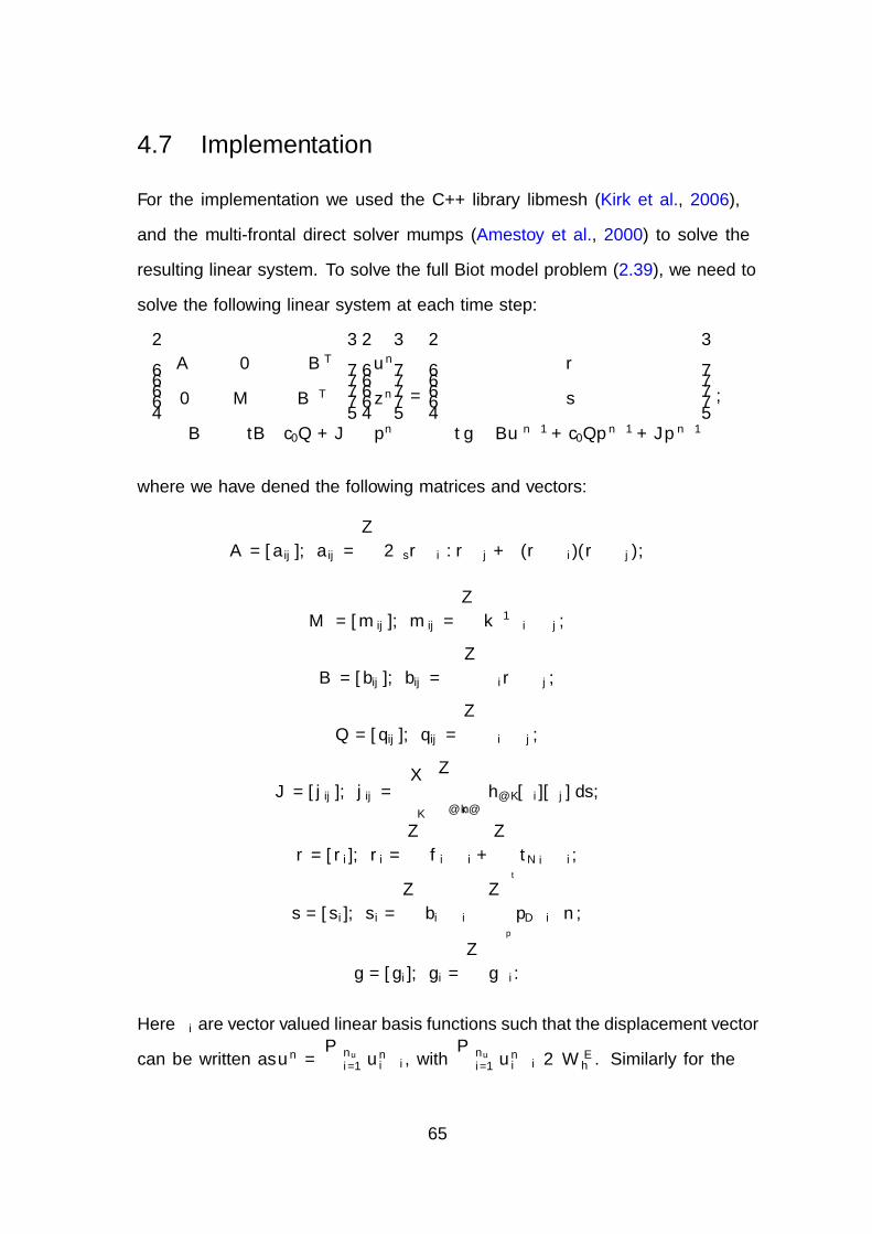
4.7 Implementation

For the implementation we used the C++ library libmesh (Kirk et al., 2006),

and the multi-frontal direct solver mumps (Amestoy et al., 2000) to solve the

resulting linear system. To solve the full Biot model problem (2.39), we need to

solve the following linear system at each time step:

A 0 αBT

0 M BT

−αB −∆tB c0Q+ J

un

zn

pn

=

r

s

∆t g −Bun−1 + c0Qpn−1 + Jpn−1

,

where we have defined the following matrices and vectors:

A = [aij], aij =

∫Ω

2µs∇φi : ∇φj + λ(∇ · φi)(∇ · φj),

M = [mij], mij =

∫Ω

k−1φi · φj,

B = [bij], bij = −∫

Ω

ψi∇ · φj,

Q = [qij], qij =

∫Ω

ψi · ψj,

J = [jij], jij = δ∑K

∫∂k\∂Ω

h∂K [ψi][ψj] ds,

r = [ri], ri =

∫Ω

fi · φi +

∫Γt

tNi · φi,

s = [si], si =

∫Ω

bi · φi −∫

Γp

pDφi · n,

g = [gi], gi =

∫Ω

gψi.

Here φi are vector valued linear basis functions such that the displacement vector

can be written as un =∑nu

i=1 uni φi, with

∑nui=1 u

ni φi ∈ W E

h . Similarly for the

65

relative fluid vector we have zn =∑nz

i=1 zni φi, with

∑nzi=1 z

ni φi ∈ WD

h . The

scalar valued constant basis functions ψi are used to approximate the pressure,

such that pn =∑np

i=1 pni ψi, with

∑npi=1 p

ni ψi ∈ Qh.

4.7.1 Algorithm to assemble the stabilisation matrix

Let K ∈ Th be an element and D(K) be the pressure degree of freedom associated

with element K. We define A(K) to be the set of elements L ∈ Th neighbouring

K.

Algorithm 1 Stabilisation matrix J assembly

for every K ∈ Th do

for every L ∈ A(K) do

Calculate h∂K

i← D(K)

j ← D(L)

Jii ← Jii + (δh∂K in 2D, δh3/2∂K in 3D)

Jij ← Jij − (δh∂K in 2D, δh3/2∂K in 3D)

end for

end for

4.8 Numerical Results

We first present convergence studies for both two- and three-dimensional test

problems which illustrate the predicted convergence rates for the fully-discrete

finite element method. We then apply our method to the popular 2D cantilever

bracket problem and demonstrate that our stabilisation techniques overcomes

the spurious pressure oscillations that have been experienced by other methods.

Finally, a 3D unconfined compression problem is presented that highlights the

66

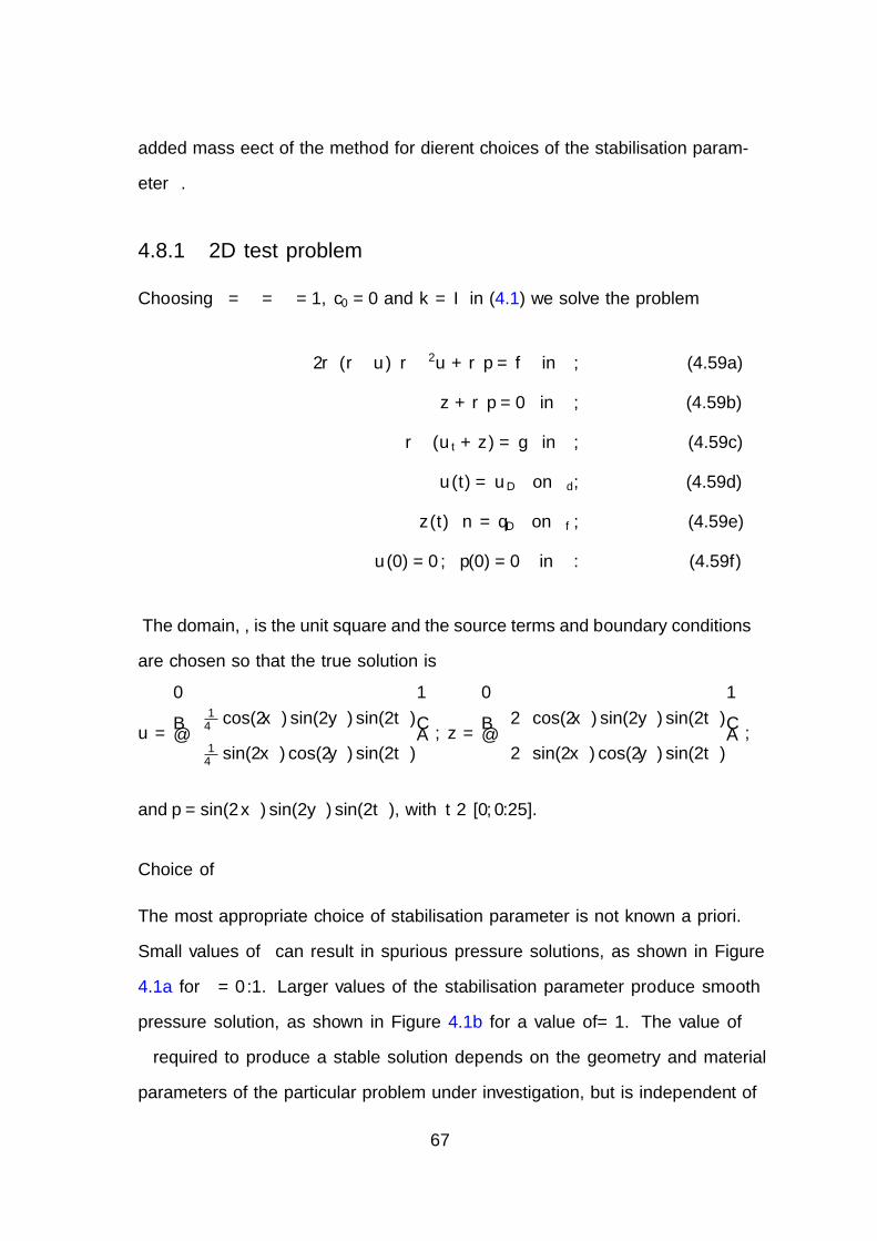
added mass effect of the method for different choices of the stabilisation param-

eter δ.

4.8.1 2D test problem

Choosing λ = µ = α = 1, c0 = 0 and k = I in (4.1) we solve the problem

−2∇ (∇ · u)−∇2u+∇p = f in Ω, (4.59a)

z +∇p = 0 in Ω, (4.59b)

∇ · (ut + z) = g in Ω, (4.59c)

u(t) = uD on Γd, (4.59d)

z(t) · n = qD on Γf , (4.59e)

u(0) = 0, p(0) = 0 in Ω. (4.59f)

The domain, Ω, is the unit square and the source terms and boundary conditions

are chosen so that the true solution is

u =

− 14π

cos(2πx) sin(2πy) sin(2πt)

− 14π

sin(2πx) cos(2πy) sin(2πt)

, z =

−2π cos(2πx) sin(2πy) sin(2πt)

−2π sin(2πx) cos(2πy) sin(2πt)

,

and p = sin(2πx) sin(2πy) sin(2πt), with t ∈ [0, 0.25].

Choice of δ

The most appropriate choice of stabilisation parameter δ is not known a priori.

Small values of δ can result in spurious pressure solutions, as shown in Figure

4.1a for δ = 0.1. Larger values of the stabilisation parameter produce smooth

pressure solution, as shown in Figure 4.1b for a value of δ = 1. The value of

δ required to produce a stable solution depends on the geometry and material

parameters of the particular problem under investigation, but is independent of

67

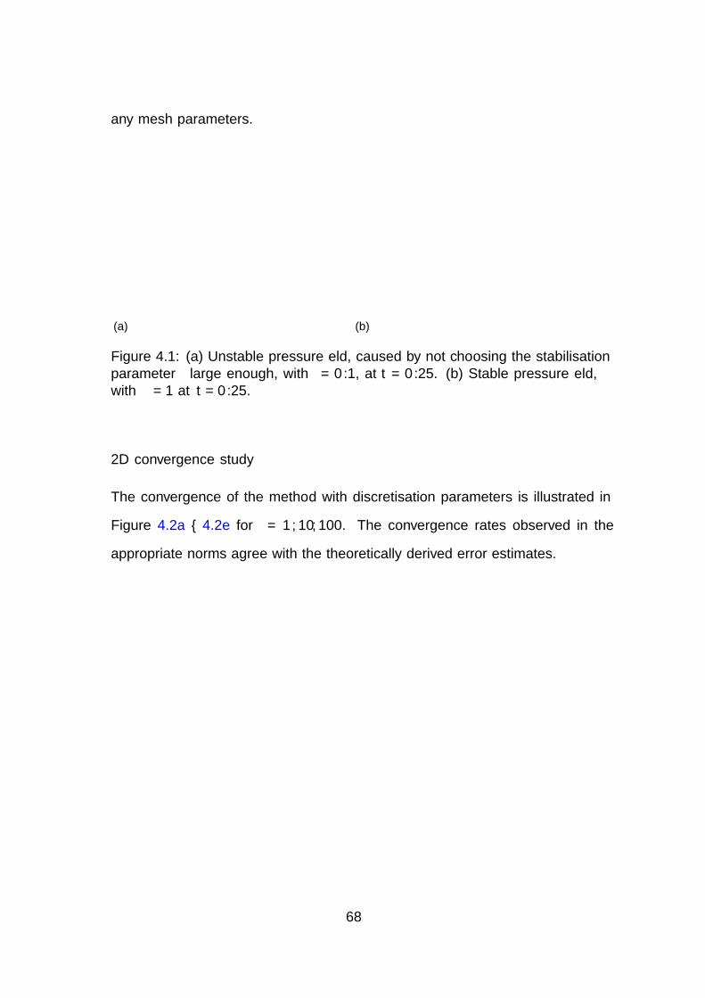
any mesh parameters.

(a)

-21.1

14.3

-20.0

-10.0

0.00

10.0

Pressure

(b)

-1.01

0.857

-0.800

-0.400

0.00

0.400

0.800

Pressure

Figure 4.1: (a) Unstable pressure field, caused by not choosing the stabilisationparameter δ large enough, with δ = 0.1, at t = 0.25. (b) Stable pressure field,with δ = 1 at t = 0.25.

2D convergence study

The convergence of the method with discretisation parameters is illustrated in

Figure 4.2a – 4.2e for δ = 1, 10, 100. The convergence rates observed in the

appropriate norms agree with the theoretically derived error estimates.

68

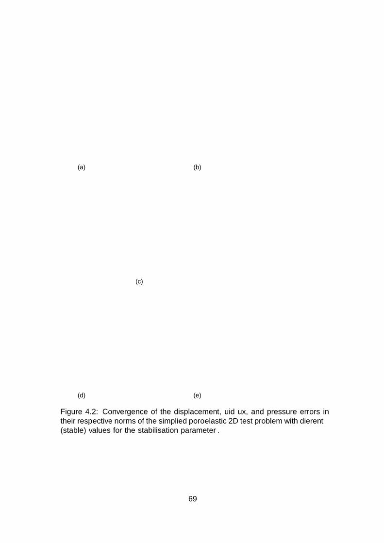
(a)

2 3 4 5 6 7 8 9−8

−7

−6

−5

−4

−3

−2

−1

0

1

2D convergence of ||u− uh||L∞(H 1)

log(1/∆t), log(1/∆h)

log(error)

δ = 1

δ = 10

δ = 100

1st order

(b)

2 3 4 5 6 7 8 9−4

−3

−2

−1

0

1

2

3

4

5

2D convergence of ||∇ · (z − zh)||L2(L2)

log(1/∆t), log(1/∆h)

log(error)

δ = 1

δ = 10

δ = 100

1st order

(c)

2 3 4 5 6 7 8 9−9

−8

−7

−6

−5

−4

−3

−2

−1

0

1

2D convergence of ||p− ph||L∞(L2)

log(1/∆t), log(1/∆h)

log(error)

δ = 1

δ = 10

δ = 100

1st order

(d)

2 3 4 5 6 7 8 9−17

−16

−15

−14

−13

−12

−11

−10

−9

−8

−7

−6

−5

−4

2D convergence of ||u− uh||L2(L2 )

log(1/∆t), log(1/∆h)

log(error)

δ = 1

δ = 10

δ = 100

2nd order

(e)

2 3 4 5 6 7 8 9−11

−10

−9

−8

−7

−6

−5

−4

−3

−2

−1

0

1

2

3

2D convergence of ||z− zh||L2(L2 )

log(1/∆t), log(1/∆h)

log(error)

δ = 1

δ = 10

δ = 100

2nd order

Figure 4.2: Convergence of the displacement, fluid flux, and pressure errors intheir respective norms of the simplified poroelastic 2D test problem with different(stable) values for the stabilisation parameter δ.

69

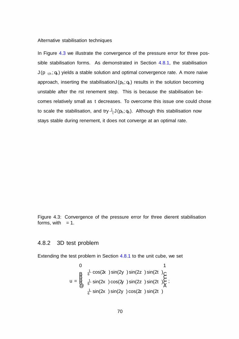
Alternative stabilisation techniques

In Figure 4.3 we illustrate the convergence of the pressure error for three pos-

sible stabilisation forms. As demonstrated in Section 4.8.1, the stabilisation

J(p∆t,h, qh) yields a stable solution and optimal convergence rate. A more naive

approach, inserting the stabilisation J(ph, qh) results in the solution becoming

unstable after the first refinement step. This is because the stabilisation be-

comes relatively small as ∆t decreases. To overcome this issue one could chose

to scale the stabilisation, and try 1∆tJ(ph, qh). Although this stabilisation now

stays stable during refinement, it does not converge at an optimal rate.

3 4 5 6−6

−5

−4

−3

−2

−1

2D convergence of ||p− ph||l∞(L2)

log(1/∆t), log(1/∆h)

log(error)

J (pδt,h, qh)

J (ph, qh)1∆tJ(ph, qh)

1st order

Figure 4.3: Convergence of the pressure error for three different stabilisationforms, with δ = 1.

4.8.2 3D test problem

Extending the test problem in Section 4.8.1 to the unit cube, we set

u =

− 1

6πcos(2πx) sin(2πy) sin(2πz) sin(2πt)

− 16π

sin(2πx) cos(2πy) sin(2πz) sin(2πt)

− 16π

sin(2πx) sin(2πy) cos(2πz) sin(2πt)

,

70

z =

−2π cos(2πx) sin(2πy) sin(2πz) sin(2πt)

−2π sin(2πx) cos(2πy) sin(2πz) sin(2πt)

−2π sin(2πx) sin(2πy) cos(2πz) sin(2πt)

,

and

p = sin(2πx) sin(2πy) sin(2πz) sin(2πt).

The expected rates of convergence for each variable in the appropriate norm

are illustrated in the numerical results presented in figure 4.4a – 4.4e for δ =

0.001, 0.01, 0.1. The stabilisation factor δ may be chosen to be very much smaller

for 3D problems as compared to 2D problems and the effect of the stabilisation

term on the solution is negligible. This can be explained by the improved ratio

of solid displacement and fluid flux nodes to pressure nodes in three dimensions,

making the LBB condition easier to satisfy.

71

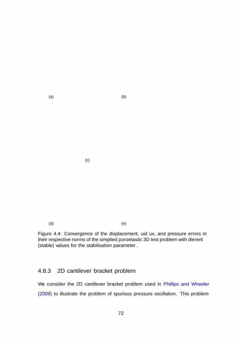
(a)

1 2 3 4 5−6

−5

−4

−3

−2

−1

0

3D convergence of ||u− uh||L∞(H 1)

log(1/∆t), log(1/∆h)

log(error)

δ = 0.001

δ = 0.01

δ = 0.1

1st order

(b)

2 3 4 5−1

0

1

2

3

4

3D convergence of ||∇ · (z − zh)||L2(L2)

log(1/∆t), log(1/∆h)

log(error)

δ = 0.001

δ = 0.01

δ = 0.1

1st order

(c)

2 3 4 5−5

−4

−3

−2

−1

0

1

2

3D convergence of ||p− ph||L∞(L2)

log(1/∆t), log(1/∆h)

log(error)

δ = 0.001

δ = 0.01

δ = 0.1

1st order

(d)

2 3 4 5−13

−12

−11

−10

−9

−8

−7

−6

−5

3D convergence of ||u− uh||L2(L2 )

log(1/∆t), log(1/∆h)

log(error)

δ = 0.001

δ = 0.01

δ = 0.1

2nd order

(e)

2 3 4 5−6

−5

−4

−3

−2

−1

0

1

2

3D convergence of ||z− zh||L2(L2 )

log(1/∆t), log(1/∆h)

log(error)

δ = 0.001

δ = 0.01

δ = 0.1

2nd order

Figure 4.4: Convergence of the displacement, fluid flux, and pressure errors intheir respective norms of the simplified poroelastic 3D test problem with different(stable) values for the stabilisation parameter δ.

4.8.3 2D cantilever bracket problem

We consider the 2D cantilever bracket problem used in Phillips and Wheeler

(2009) to illustrate the problem of spurious pressure oscillation. This problem

72

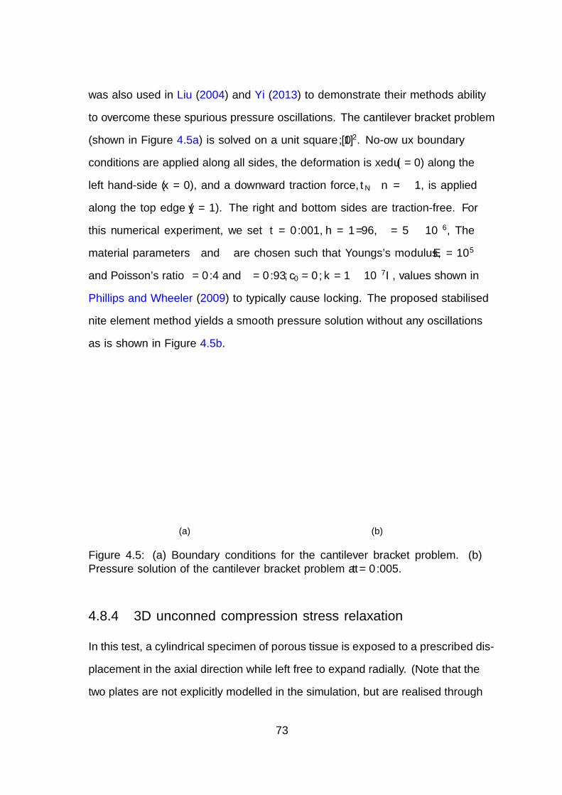
was also used in Liu (2004) and Yi (2013) to demonstrate their methods ability

to overcome these spurious pressure oscillations. The cantilever bracket problem

(shown in Figure 4.5a) is solved on a unit square [0, 1]2. No-flow flux boundary

conditions are applied along all sides, the deformation is fixed (u = 0) along the

left hand-side (x = 0), and a downward traction force, tN · n = −1, is applied

along the top edge (y = 1). The right and bottom sides are traction-free. For

this numerical experiment, we set ∆t = 0.001, h = 1/96, δ = 5 × 10−6, The

material parameters λ and µ are chosen such that Youngs’s modulus, E = 105

and Poisson’s ratio ν = 0.4 and α = 0.93, c0 = 0,k = 1× 10−7I, values shown in

Phillips and Wheeler (2009) to typically cause locking. The proposed stabilised

finite element method yields a smooth pressure solution without any oscillations

as is shown in Figure 4.5b.

Ωu = (0, 0)Tz · n = 0 z · n = 0

z · n = 0

z · n = 0t · n = −1

(a)

0 0.1 0.2 0.3 0.4 0.5 0.6 0.7 0.8 0.9 1−0.4

−0.2

0

0.2

0.4

0.6

0.8

1

y

Pressure

x=0.25

x=0.5

x=0.75

(b)

Figure 4.5: (a) Boundary conditions for the cantilever bracket problem. (b)Pressure solution of the cantilever bracket problem at t = 0.005.

4.8.4 3D unconfined compression stress relaxation

In this test, a cylindrical specimen of porous tissue is exposed to a prescribed dis-

placement in the axial direction while left free to expand radially. (Note that the

two plates are not explicitly modelled in the simulation, but are realised through

73

displacement boundary conditions.) After loading the tissue, the displacement

is held constant while the tissue relaxes in the radial direction due to interstitial

fluid flow through the radial boundary. For the special case of a cylindrical ge-

ometry Armstrong et al. (1984) found a closed-form analytical solution for the

radial displacement u given by

u

a(a, t) = ε0

[ν + (1− 2ν)(1− ν)

∞∑n=1

exp (−α2nMkta2 )

α2n(1− ν)2 − (1− ν)

]. (4.60)

where αn are the solutions to the characteristic equation J1(x)−(1−ν)xJ0(x)/(1−

2ν) = 0, where J0 and J1 are Bessel functions, ε0 is the amplitude of the applied

axial strain, a is the radius of the cylinder, and tg is the characteristic time of

diffusion (relaxation) tg = a2/Mk, where M = λ+ 2µ is the P-wave modulus of

the elastic solid skeleton, and k is the permeability.

The analytical solution available for this test problem describes the displace-

ment of the outer radius which is directly dependent on the amount of mass in

the system since the porous medium is assumed to be incompressible and fully

saturated. It is therefore an ideal test problem for analyzing the effect that the

added stabilisation term has on the conservation of mass. In Figure 5.2 we can

see that for large values of δ the numerical solution loses mass faster and comes

to a steady state that has less mass than the analytical solution. This is a clear

limitation of the method and the stability parameter therefore needs to be chosen

carefully. However, for 3D problems δ can be chosen to be very small so this

effect is negligible, as can be seen in Figure 5.2 for a stable value of δ = 0.001.

74

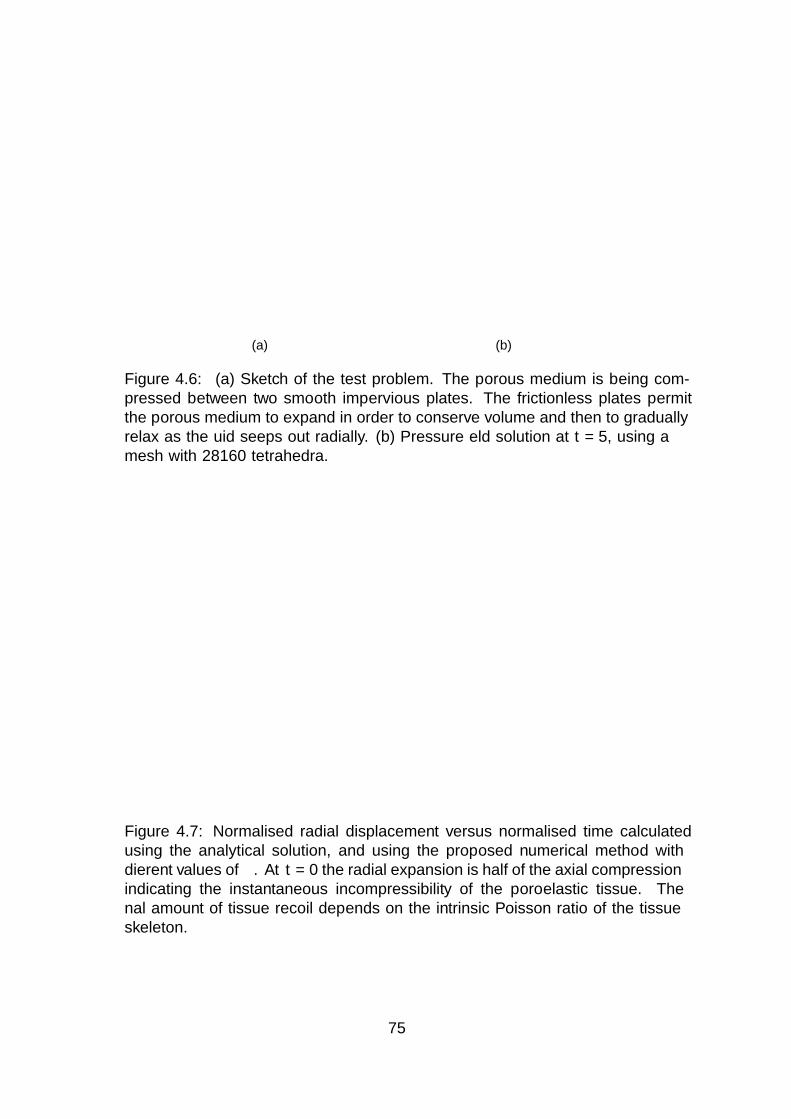
Impervious smooth plate

Specimen

Compression direction

Flow direction

(a)

-6.804e-5

0

0.002

0.004

Pressure

0.0051662

(b)

Figure 4.6: (a) Sketch of the test problem. The porous medium is being com-pressed between two smooth impervious plates. The frictionless plates permitthe porous medium to expand in order to conserve volume and then to graduallyrelax as the fluid seeps out radially. (b) Pressure field solution at t = 5, using amesh with 28160 tetrahedra.

0 0.2 0.4 0.6 0.8 1 1.20.1

0.15

0.2

0.25

0.3

0.35

0.4

0.45

0.5

Unconfined compression relaxation test

Nondimensional time (t/tg)

Radialdisplacemen

t(u/aǫ0)

Analytical solution

Numerical solution, δ=0.001 .

Numerical solution, δ=0.1

Numerical solution, δ=1

Figure 4.7: Normalised radial displacement versus normalised time calculatedusing the analytical solution, and using the proposed numerical method withdifferent values of δ. At t = 0 the radial expansion is half of the axial compressionindicating the instantaneous incompressibility of the poroelastic tissue. Thefinal amount of tissue recoil depends on the intrinsic Poisson ratio of the tissueskeleton.

75

4.9 Conclusion

The local pressure jump stabilisation method (Burman and Hansbo, 2007) is

commonly used to solve the Stokes or Darcy equations using piecewise linear

approximations for the velocities, and piecewise constant approximations for the

pressure variable. The main contribution of this chapter has been to extend

these ideas to three-field poroelasticity. We have presented a stability result

for the discretised equations that guarantees the existence of a unique solution

at each time step, and derived an energy estimate which can be used to prove

weak convergence of the solution to the discretised system to the solution to

the continuous problem as the mesh parameters tend to zero. We also derived

an optimal error estimate which includes an error for the fluid flux in its nat-

ural Hdiv norm. We have also presented numerical experiments in 2D and 3D

that illustrate the convergence of the method, the effectiveness of the method

in overcoming spurious pressure oscillations, and the added mass effect of the

stabilisation term.

76

Chapter 5

A stabilised finite element

method for poroelasticity valid in

large deformations

5.1 Introduction

In Chapter 4, we developed a stabilised, low-order, mixed finite-element method

for the fully saturated, incompressible, poroelasticity equations, in the linear,

small deformation case. In this Chapter we extend this work to the nonlinear,

large deformation case.

In section 5.2, we recall the large deformation quasi-static incompressible

poroelastic model. In section 5.3 we present the stabilised nonlinear finite-

element method, and provide some implementation details in section 5.4. In

section 5.5, we present a range of 3D numerical experiments to verify the accu-

racy of the method and illustrate its ability to reliably capture steep pressure

gradients.

77

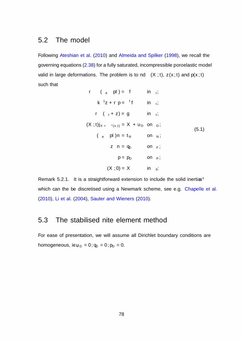
5.2 The model

Following Ateshian et al. (2010) and Almeida and Spilker (1998), we recall the

governing equations (2.38) for a fully saturated, incompressible poroelastic model

valid in large deformations. The problem is to find χ(X, t), z(x, t) and p(x, t)

such that

−∇ · (σe − pI) = ρf

k−1z +∇p = ρff

∇ · (χt + z) = g

χ(X, t)|X=χ−1(x,t) = X + uD

(σe − pI)n = tN

z · n = qD

p = pD

χ(X, 0) = X

in Ωt,

in Ωt,

in Ωt,

on ΓD,

on ΓN ,

on ΓF ,

on ΓP ,

in Ω0.

(5.1)

Remark 5.2.1. It is a straightforward extension to include the solid inertia as

which can the be discretised using a Newmark scheme, see e.g. Chapelle et al.

(2010), Li et al. (2004), Sauter and Wieners (2010).

5.3 The stabilised finite element method

For ease of presentation, we will assume all Dirichlet boundary conditions are

homogeneous, ie., uD = 0, qD = 0, pD = 0.

78

5.3.1 Weak formulation

We define the following spaces for deformed location, fluid flux and pressure

respectively,

W E(Ωt) = v ∈ (H1(Ωt))d : v = 0 on ΓD,

WD(Ωt) = w ∈ Hdiv(Ωt) : w · n = 0 on ΓF,

L(Ωt) =

L2(Ωt) if ΓN ∪ ΓP 6= ∅

L20(Ωt) if ΓN ∪ ΓP = ∅,

,

where L20(Ωt) =

q ∈ L2(Ωt) :

∫Ωtq dx = 0

.

We make use of the identity ∇·(σev) = ∇·σe ·v−σe : ∇v, and the symmetry

of σe to yield the following continuous weak problem. Find χ(X, t) ∈W E(Ωt),

z(x, t) ∈WD(Ωt) and p(x, t) ∈ L(Ωt) for any time t ∈ [0, T ] such that

∫Ωt

[σe : ∇Sv − p∇ · v

]dΩt =

∫Ωt

ρf · v dΩt

+

∫ΓN (t)

tN · v dΓN(t) ∀v ∈W E(Ωt),∫Ωt

[k−1z ·w − p∇ ·w

]dΩt =

∫Ωt

ρff ·w dΩt ∀w ∈WD(Ωt),∫Ωt

[q∇ · χt + q∇ · z] dΩt =

∫Ωt

gq dΩt ∀q ∈ L(Ωt).

(5.2)

Here ∇Sv = 12

(∇v + (∇v)T

)for some vector v.

5.3.2 The fully discrete model

Let T h be a partition of Ωt into non-overlapping elements K, where h denotes

the size of the largest element in T h. We define the following finite element

79

spaces,

W Eh =

vh ∈ C0(Ωt) : vh|K ∈ P1(K) ∀K ∈ T h,vh = 0 on ΓD

,

WDh =

wh ∈ C0(Ωt) : wh|K ∈ P1(K) ∀K ∈ T h,wh · n = 0 on ΓF

,

Qh =

qh : qh|K ∈ P0(K) ∀K ∈ T h

if ΓN ∪ Γp 6= ∅

qh : qh|K ∈ P0(K),∫

Ωtqh = 0 ∀K ∈ T h

if ΓN ∪ Γp = ∅

,

where P0(K) and P1(K) are respectively the spaces of constant and linear poly-

nomials on K.

We define the combined solution space Uh(t) = W Eh × WD

h × Qh. The

discretisation in time is given by partitioning [0, T ] into N evenly spaced non-

overlapping regions (tn−1, tn], n = 1, 2, . . . , N , where tn − tn−1 = ∆t. For any

sufficiently smooth function v(t, x) we define vn(x) = v(x, tn) and the discrete

time derivative by vn∆t := vn−vn−1

∆t. The fully discrete weak problem is: For

n = 1, . . . , N , find χnh ∈W Eh (Ωtn), znh ∈WD

h (Ωtn) and pnh ∈ Qh(Ωtn) such that

∫Ωtn

[σne,h : ∇Svh − pnh∇ · vh

]dΩtn =

∫Ωtn

ρfn · vh dΩtn

+

∫ΓN (tn)

tnN · vh dΓN(tn) ∀vh ∈W Eh (Ωtn),∫

Ωtn

[k−1znh ·wh − pnh∇ ·wh

]dΩtn =

∫Ωtn

ρffn ·wh dΩtn ∀wh ∈WDh (Ωtn),∫

Ωtn

[qh∇ · χn∆t,h + qh∇ · znh

]dΩtn + J(pn∆t,h, qh) =

∫Ωtn

gnqh dΩtn

∀qh ∈ Qh(Ωtn). (5.3)

5.3.3 Solution via Newton iteration at tn

Since the system of equations (5.3) is highly nonlinear, its solution requires a

scheme such as Newton’s method. With Newton’s method, an improved solution

80

is obtained from a linear approximation of the nonlinear equation at an already

computed solution. This first order Taylor expansion corresponds in finite ele-

ment applications to the linearisation of the weak form, and can be obtained by

the directional derivative, explained in section 5.3.4.

Let unh = χnh, znh , pnh ∈ Uh(tn) denote the solution vector at a particular

time step, ξuh = ξχh, ξzh, ξph denote the solution increment vector, and vh =

vh,wh, qh ∈ Vh(t) where Vh(t) = W Eh0 ×WD

h0 × Qh. The nonlinear system of

equations (5.3) can be recast in the form: Find unh ∈ Uh(tn) such that

Gn(unh, vh) = 0 ∀vh ∈ Vh(tn), (5.4)

where

Gn(unh, vh) =

∫Ωtn

(σne,h : ∇Svh − pnh∇ · vh + k−1znh ·wh − pnh∇ ·wh

+qh∇ · (χn∆t,h + znh)− ρfn · vh + ρffn ·wh + gqh)

dΩtn

−∫

ΓN (tn)

tnN · vh dΓN(tn).

(5.5)

Given an approximate solution unh, we approximate (5.4) by

Gn(unh, vh) +DGn(unh, vh)[ξuh] = 0 ∀vh ∈ Vh(tn),

and solve

DGn(unh, vh)[ξuh] = −G(unh, vh) ∀vh ∈ Vh(tn), (5.6)

for the Newton step ξuh, where DG is the directional derivative of G, at unh, in

the direction ξuh.

81

5.3.4 Approximation of DGn.

In biphasic tissue problems, it is common to approximate directional derivative

of G by assuming the nonlinear elasticity term is the dominant nonlinearity and

ignoring the other nonlinearities (Un and Spilker, 2006; White and Borja, 2008).

Let

En((χnh, pnh),vh) =

∫Ωtn

σne,h : ∇Svh − pnh∇ · vh dΩtn . (5.7)

For Newton’s method we require the directional derivative of En((χn∆t,h, pnh),vh)

at a particular trial solution (χn∆t,h, pnh) in the direction ξχh, given by (see Wrig-

gers (2008, section 3.5.3))

DEn((χnh, pnh),vh)[ξχh] =

∫Ωtn

∇Svh : Θnh : ∇Sξχh+σne,h :

((∇ξχh)T · ∇vh

)dΩtn ,

(5.8)

where Θnh is a fourth-order tensor and σne,h is the effective (elastic) stress tensor,

both evaluated at a trial solution χnh. Further, any variable with a bar above

it will correspond to it being evaluated at a trial solution. The fourth-order

spatial tangent modulus tensor Θ is described in A.1. For a detailed explanation

and derivation see Bonet and Wood (1997); Wriggers (2008). The approximate

linearisation of the nonlinear problem is thus given by

DGn(unh, vh)[ξuh] ≈∫Ωtn

[∇Svh : Θn

h : ∇Sξχh + σe,h :((∇ξχh)T · ∇vh

)− ξph∇ · vh

+k−1ξzh ·wh − ξph∇ ·wh + qh∇ ·(ξχh∆t

+ ξzh

)]dΩtn ,

(5.9)

82

Using (5.5), (5.9) and equation (5.6) the Newton solve becomes: Find

ξχh ∈W Eh (Ωtn), ξzh ∈WD

h (Ωtn) and ξph ∈ Qh(Ωtn) such that

∫Ωtn

[∇Svh : Θn

h : ∇Sξχh + σne,h :((∇ξχh)T · ∇vh

)− ξph∇ · vh

]dΩtn

=

∫Ωtn

[σne,h : ∇Svh − pnh∇ · vh − ρfn · vh

]dΩtn

−∫

Γn(tn)

tnN · vh dΓn(tn) ∀vh ∈W Eh (Ωtn),∫

Ωtn

[k−1ξzh ·wh − ξph∇ ·wh

]dΩtn

=

∫Ωtn

[k−1znh ·wh − pnh · ∇wh − ρffn ·wh

]dΩtn ∀wh ∈WD

h (Ωtn),∫Ωtn

[qh∇ ·

(ξχh∆t

+ ξzh

)]dΩtn + J

(ξph∆t

, qh

)=

∫Ωtn

[qh∇ · (χn∆t,h + zh)− gqh

]dΩtn + J (p∆t,h, qh) ∀qh ∈ Qh(Ωtn).

(5.10)

5.4 Implementation details

5.4.1 Newton algorithm

We will now let uni := χni , zni , pni denote the fully discrete solution at the

ith step within the Newton method at time tn. To ease the notation, we have

suppressed the lower case h, previously used to denote the spatial discretisation.

To solve the nonlinear poroelastic problem using Newton’s method at a particular

time step, we perform the steps outlined in Algorithm 2.

83

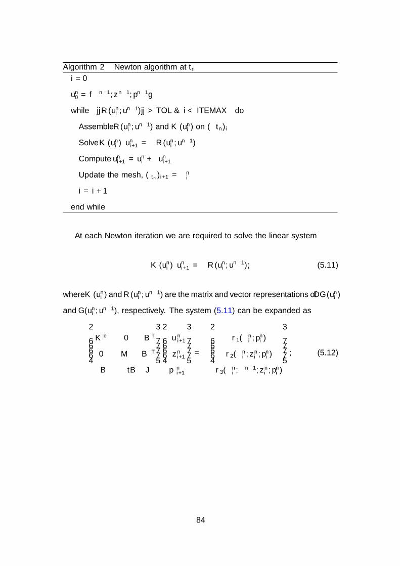
Algorithm 2 Newton algorithm at tn

i = 0

un0 = χn−1, zn−1, pn−1

while ||R(uni , un−1)|| > TOL & i < ITEMAX do

Assemble R(uni , un−1) and K(uni ) on Ω(tn)i

Solve K(uni )δuni+1 = −R(uni , un−1)

Compute uni+1 = uni + δuni+1

Update the mesh, (Ωtn)i+1 = χni

i = i+ 1

end while

At each Newton iteration we are required to solve the linear system

K(uni )ξuni+1 = −R(uni , un−1), (5.11)

whereK(uni ) andR(uni , un−1) are the matrix and vector representations ofDG(uni )

and G(uni , un−1), respectively. The system (5.11) can be expanded as

Ke 0 BT

0 M BT

−B −∆tB J

ξuni+1

ξzni+1

ξpni+1

= −

r1(χni , p

ni )

r2(χni , zni , p

ni )

r3(χni ,χn−1, zni , p

ni )

, (5.12)

84

where the elements in the matrices in (5.12) are given by

kekl =

∫(Ωtn )i

ETkD(χni )El + (∇φk)Tσe(χni )∇φl d(Ωtn)i,

mkl =

∫(Ωtn )i

k−1(χni )φk · φl d(Ωtn)i,

bkl = −∫

(Ωtn )i

ψk∇ · φl d(Ωtn)i,

jkl = δ∑K∈T hi

∫∂K\∂(Ωtn )i

h∂K [ψk][ψl] ds.

r1l =

∫(Ωtn )i

(σe(χni )− pni I) : ∇φl − ρ(χni )φl · f d(Ωtn)i

−∫

(ΓN )i

φl · tN(χni ) d(ΓN)i,

r2l =

∫(Ωtn )i

k−1(χni )φl · zni − pni∇ · φl − ρf (χni )φl · f d(Ωtn)i,

r3l =

∫(Ωtn )i

ψl∇ ·(χni − χn−1

)+ ∆tψl∇ · zni −∆tψlg d(Ωtn)i

+δ∑K∈T h

∫∂K\∂(Ωtn )i

h∂K [ψl][pni − pn−1] ds.

Here φk are vector valued linear basis functions such that the displacement vector

at the ith iteration can be written as χni =∑nχ

k=1χni,kφk, with∑nχ

k=1χni,kφk ∈W E

h . Similarly for the fluid flux vector we have zni =∑nz

k=1 zni,kφk,

with∑nz

k=1 zni,kφk ∈WD

h . The scalar valued constant basis functions ψi are used

to approximate the pressure, such that pni =∑np

k=1 pni,kψk, with

∑npk=1 p

ni,kψk ∈ Qh.

Also to aid the assembly of the fourth order tensor we have adopted the matrix

voigt notation. In particular D is the matrix form of Θ, and Ek is the matrix

version of ∇Sφk, see (A.3) and (A.4) for details.

5.4.2 Fluid-flux boundary condition

When solving the equations for Darcy flow using the Raviart-Thomas element

(RT-P0), the fluid-flux boundary condition is enforced naturally by this diver-

85

gence free element. Unfortunately this is not possible using our proposed P1-P1-

P0-stabilised element. However, solving the poroelastic equations (5.1) using a

piecewise linear approximation for the deformation and Raviart-Thomas element

for the fluid (P1-RT-P0) does not satisfy the discrete inf-sup condition and can

yield spurious pressure oscillations, see Phillips and Wheeler (2008, 2009) for

details.

To enforce the no-flux boundary condition z ·n = qD we introduce a Lagrange

multiplier Λ along the boundary ΓF . Let W F = l ∈ Hdiv(ΓF ,R). The resulting

modified continuous weak-form is now:

G((u, z, p)), (v,w, q)) + (Λ,w · n)ΓF = qD ∀(v,w, q) ∈W E(Ωt),WD(Ωt),L(Ωt),

(z · n, l)ΓF = qD, ∀l ∈ W F .

(5.13)

The discretisation and implementation of this additional constraint is straight-

forward and results in a linear system with additional degrees of freedom for

every node on ΓF . The terms (Λ,w ·n)ΓF and (z ·n, l)ΓF are nonlinear since the

normal is a function of the displacement. We have found that linearising these

terms using a Picard type linearisation (lagging) does not affect the convergence

of the Newton algorithm. Alternatively these terms could be linearised explicitly

as has been described in detail for the traction boundary condition, see Wriggers

(2008, section 4.2.5) and Ateshian et al. (2010).

5.5 Numerical results

We present four numerical examples to test the performance of the proposed sta-

bilised finite element method. The first two examples are from mechanobiology

and geotechnical applications, the third is a swelling example that undergoes

significant large deformations and the fourth is an application from respiratory

86

physiology. For the implementation we used the C++ library libmesh (Kirk

et al., 2006), and the multi-frontal direct solver mumps (Amestoy et al., 2000)

to solve the resulting linear systems. For the strain energy law we chose a Neo-

Hookean law taken from Wriggers (2008, eqn. (3.119)), with the penalty term

chosen such that 0 ≤ φ < 1, namely

W (C) =µ

2(tr(C)− 3) +

λ

4(J2 − 1)− (µ+

λ

2)ln(J − 1 + φ0). (5.14)

For further discussion on strain energy laws for porelasticity we refer to Chapelle

and Moireau (2014) and Vuong et al. (2015). The material parameters µ and λ

in (5.14) can be related to the Young’s modulus E and the Poisson ratio ν by

µ = E/(2(1 + ν)) and λ = (Eν)/((1 + ν)(1− 2ν)). Details of the effective stress

tensor and fourth-order spatial tangent modulus for this particular law can be

found in A.3. For the permeability law we chose

k0(C) = k0I. (5.15)

5.5.1 3D unconfined compression stress relaxation

In this test, a cylindrical specimen of porous tissue is exposed to a prescribed

displacement in the axial direction while left free to expand radially. The origi-

nal experiment involved a specimen of articular cartilage being compressed via

impervious smooth plates as shown in Figure 5.1a. Note that the two plates are

not explicitly modelled in the simulation, but are realised through displacement

boundary conditions. After loading the tissue, the displacement is held constant

and the tissue is allowed to relax in the radial direction. The fluid pressure was

constrained to zero at the outer radial surface. The outer radial boundary is

permeable and free-draining, the upper and lower fluid boundaries are imper-

87

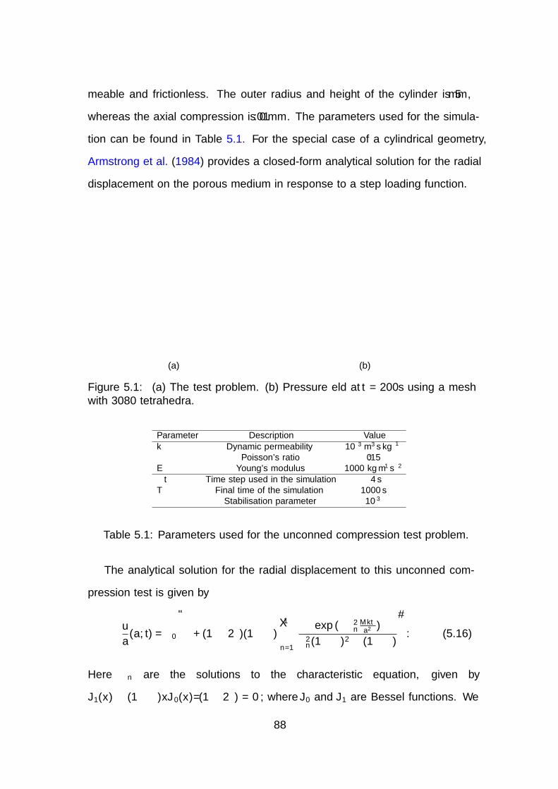
meable and frictionless. The outer radius and height of the cylinder is 5mm,

whereas the axial compression is 0.01mm. The parameters used for the simula-

tion can be found in Table 5.1. For the special case of a cylindrical geometry,

Armstrong et al. (1984) provides a closed-form analytical solution for the radial

displacement on the porous medium in response to a step loading function.

Impervious smooth plate

Specimen

Compression direction

Flow direction

(a)

0.000121

0.003474

0.001

0.002

0.003

Pressure

(b)

Figure 5.1: (a) The test problem. (b) Pressure field at t = 200s using a meshwith 3080 tetrahedra.

Parameter Description Value

k Dynamic permeability 10−3 m3 s kg−1

ν Poisson’s ratio 0.15E Young’s modulus 1000 kg m−1 s−2

∆t Time step used in the simulation 4 sT Final time of the simulation 1000 sδ Stabilisation parameter 10−3

Table 5.1: Parameters used for the unconfined compression test problem.

The analytical solution for the radial displacement to this unconfined com-

pression test is given by

u

a(a, t) = ε0

[ν + (1− 2ν)(1− ν)

∞∑n=1

exp (−α2nMkta2 )

α2n(1− ν)2 − (1− ν)

]. (5.16)

Here αn are the solutions to the characteristic equation, given by

J1(x) − (1 − ν)xJ0(x)/(1 − 2ν) = 0, where J0 and J1 are Bessel functions. We

88

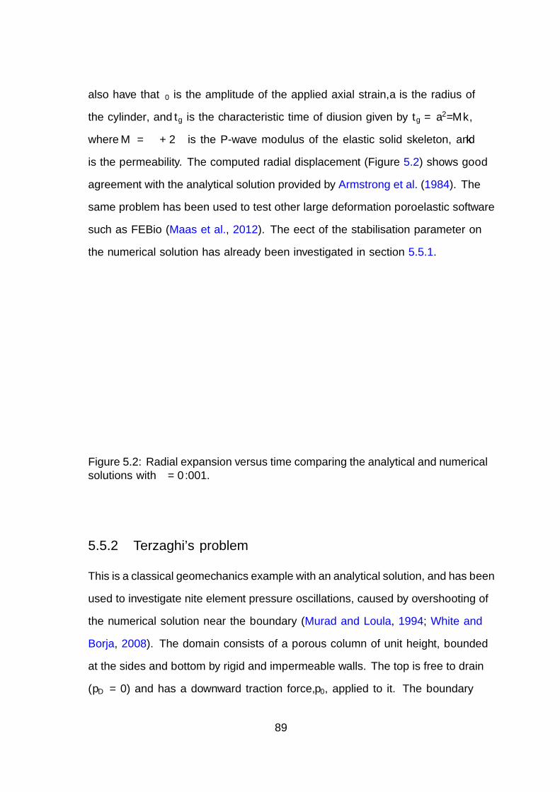
also have that ε0 is the amplitude of the applied axial strain, a is the radius of

the cylinder, and tg is the characteristic time of diffusion given by tg = a2/Mk,

where M = λ + 2µ is the P-wave modulus of the elastic solid skeleton, and k

is the permeability. The computed radial displacement (Figure 5.2) shows good

agreement with the analytical solution provided by Armstrong et al. (1984). The

same problem has been used to test other large deformation poroelastic software

such as FEBio (Maas et al., 2012). The effect of the stabilisation parameter on

the numerical solution has already been investigated in section 5.5.1.

0 0.2 0.4 0.6 0.8 1 1.20.1

0.15

0.2

0.25

0.3

0.35

0.4

0.45

0.5Unconfined compression relaxation test

Nondimensional time (t/tg)

Radialdisplacemen

t(u/aε0)

Numerical solutionAnalytical solution

Figure 5.2: Radial expansion versus time comparing the analytical and numericalsolutions with δ = 0.001.

5.5.2 Terzaghi’s problem

This is a classical geomechanics example with an analytical solution, and has been

used to investigate finite element pressure oscillations, caused by overshooting of

the numerical solution near the boundary (Murad and Loula, 1994; White and

Borja, 2008). The domain consists of a porous column of unit height, bounded

at the sides and bottom by rigid and impermeable walls. The top is free to drain

(pD = 0) and has a downward traction force, p0, applied to it. The boundary

89

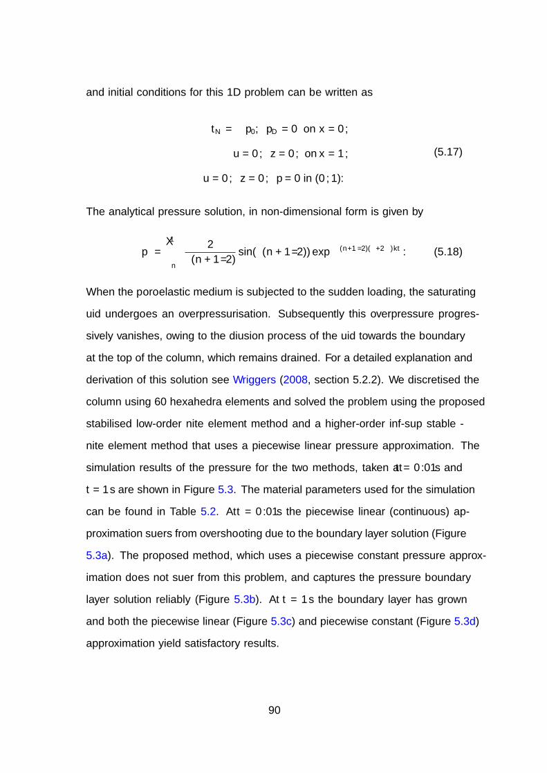
and initial conditions for this 1D problem can be written as

tN = −p0, pD = 0 on x = 0,

u = 0, z = 0, on x = 1,

u = 0, z = 0, p = 0 in (0, 1).

(5.17)

The analytical pressure solution, in non-dimensional form is given by

p∗ =∞∑n

2

π(n+ 1/2)sin(π(n+ 1/2)) exp−π(n+1/2)(λ+2µ)kt . (5.18)

When the poroelastic medium is subjected to the sudden loading, the saturating

fluid undergoes an overpressurisation. Subsequently this overpressure progres-

sively vanishes, owing to the diffusion process of the fluid towards the boundary

at the top of the column, which remains drained. For a detailed explanation and

derivation of this solution see Wriggers (2008, section 5.2.2). We discretised the

column using 60 hexahedra elements and solved the problem using the proposed

stabilised low-order finite element method and a higher-order inf-sup stable fi-

nite element method that uses a piecewise linear pressure approximation. The

simulation results of the pressure for the two methods, taken at t = 0.01s and

t = 1s are shown in Figure 5.3. The material parameters used for the simulation

can be found in Table 5.2. At t = 0.01s the piecewise linear (continuous) ap-

proximation suffers from overshooting due to the boundary layer solution (Figure

5.3a). The proposed method, which uses a piecewise constant pressure approx-

imation does not suffer from this problem, and captures the pressure boundary

layer solution reliably (Figure 5.3b). At t = 1s the boundary layer has grown

and both the piecewise linear (Figure 5.3c) and piecewise constant (Figure 5.3d)

approximation yield satisfactory results.

90

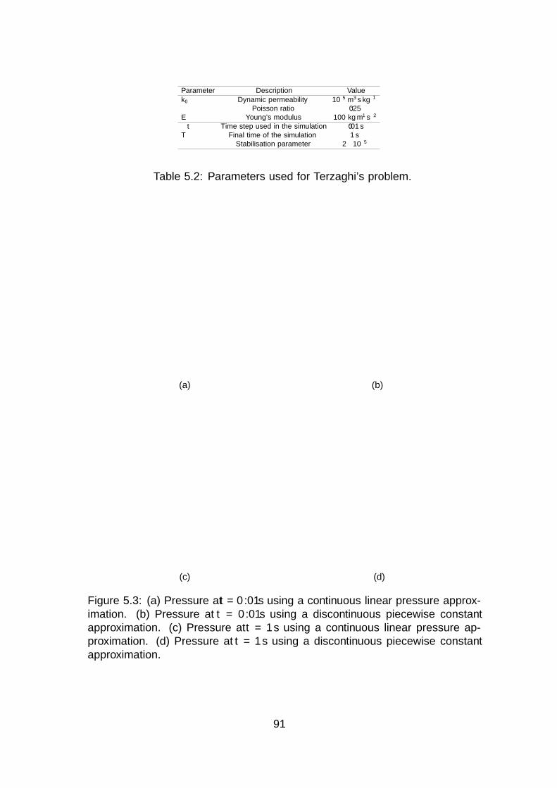
Parameter Description Value

k0 Dynamic permeability 10−5 m3 s kg−1

ν Poisson ratio 0.25E Young’s modulus 100 kg m−1 s−2

∆t Time step used in the simulation 0.01 sT Final time of the simulation 1 sδ Stabilisation parameter 2× 10−5

Table 5.2: Parameters used for Terzaghi’s problem.

0 0.2 0.4 0.6 0.8 10

0.2

0.4

0.6

0.8

1

1.2

1.4

x

p* Analytical

P1

(a)

0 0.2 0.4 0.6 0.8 10

0.2

0.4

0.6

0.8

1

1.2

1.4

x

p* Analytical

P0

(b)

0 0.2 0.4 0.6 0.8 10

0.2

0.4

0.6

0.8

1

1.2

1.4

x

p* Analytical

P1

(c)

0 0.2 0.4 0.6 0.8 10

0.2

0.4

0.6

0.8

1

1.2

1.4

x

p* Analytical

P0

(d)

Figure 5.3: (a) Pressure at t = 0.01s using a continuous linear pressure approx-imation. (b) Pressure at t = 0.01s using a discontinuous piecewise constantapproximation. (c) Pressure at t = 1s using a continuous linear pressure ap-proximation. (d) Pressure at t = 1s using a discontinuous piecewise constantapproximation.

91

5.5.3 Swelling test

This problem is similar to the one in Chapelle et al. (2010) and highlights the

method’s ability to reliably capture jumps in the pressure solution due to changes

in material parameters. Given a unit cube of material, a fluid pressure gradient

is imposed between the two opposite faces at X = 0 and X = 1. The pressure

pD on the inlet face X = 0 is increased very rapidly from zero to a limiting value

of 10kPa, i.e., pD = 104(1 − exp(−t2/0.25)) Pa). On the outlet face X = 1,

the pressure is fixed to be zero, pD = 0. There are no sources of sinks of fluid.

A zero flux condition is applied for the fluid velocity on the four other faces

(Y = 0, 1, Z = 0, 1). Normal displacements are required to be zero on the planes

X = 0, Y = 0 and Z = 0. The permeability of the cube 0 < X < 0.5, 0.5 < Y <

1, 0 < Z < 0.5 (1/8 of the volume of the unit cube) is smaller than in the rest of

the domain by a factor of 500. The computational domain shown in Figure 5.4a,

highlighting the region of reduced permeability. The parameters chosen for this

test problem are shown in Table 5.3.

Fluid enters the region from the inlet face and the material swells like a

sponge, undergoing large deformation as shown in Figure (5.4b). The evolution

of the pressure and the Jacobian at the points at (0, 0, 1), (0.5, 0, 1) and (1, 0, 1)

in the reference configuration is shown in Figures (5.5a) and (5.5b) respectively.

These position are indicated by the red, blue and green balls in Figure 5.4a. The

pressure decreases roughly linearly with x, the increase in volume also follows

a similar pattern. The pressure and volume change at the point (0, 1, 0) (black

ball in Figure 5.4a) is also shown in Figures (5.5a) and (5.5b). Due to its re-

duced permeability this region is much slower to swell and achieve its ultimate

equilibrium state and the fluid mainly flows around the area of reduced perme-

ability, see Figure 5.4b. The steep pressure gradients at the boundary of the

less permeable region seen in Figure 5.4b are well approximated by the piecewise

92

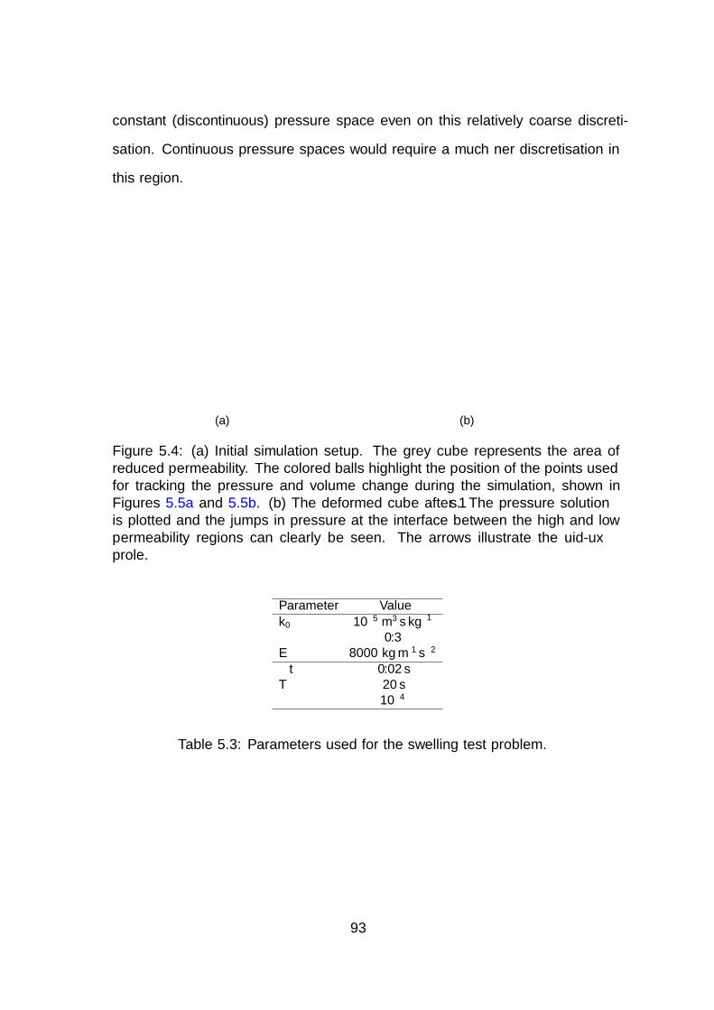
constant (discontinuous) pressure space even on this relatively coarse discreti-

sation. Continuous pressure spaces would require a much finer discretisation in

this region.

(a)

270

9450

2000

4000

6000

8000

Pressure .

(b)

Figure 5.4: (a) Initial simulation setup. The grey cube represents the area ofreduced permeability. The colored balls highlight the position of the points usedfor tracking the pressure and volume change during the simulation, shown inFigures 5.5a and 5.5b. (b) The deformed cube after 1s. The pressure solutionis plotted and the jumps in pressure at the interface between the high and lowpermeability regions can clearly be seen. The arrows illustrate the fluid-fluxprofile.

Parameter Value

k0 10−5 m3 s kg−1

ν 0.3E 8000 kg m−1 s−2

∆t 0.02 sT 20 sδ 10−4

Table 5.3: Parameters used for the swelling test problem.

93

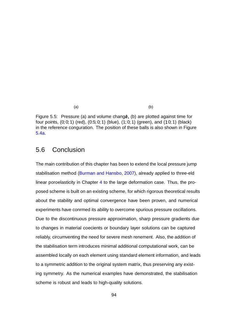
0 5 10 15 200

1000

2000

3000

4000

5000

6000

7000

8000

9000

10000

Evolution of pressure

Time (s)

Pressure

(Pa)

Black ball

Red ball

Blue ball

Green ball

(a)

0 5 10 15 201

1.5

2

2.5

3

3.5

4Evolution of Jacobian

Time (s)

J

Black ball

Red ball

Blue ball

Green ball

(b)

Figure 5.5: Pressure (a) and volume change, J , (b) are plotted against time forfour points, (0, 0, 1) (red), (0.5, 0, 1) (blue), (1, 0, 1) (green), and (1, 0, 1) (black)in the reference configuration. The position of these balls is also shown in Figure5.4a.

5.6 Conclusion

The main contribution of this chapter has been to extend the local pressure jump

stabilisation method (Burman and Hansbo, 2007), already applied to three-field

linear poroelasticity in Chapter 4 to the large deformation case. Thus, the pro-

posed scheme is built on an existing scheme, for which rigorous theoretical results

about the stability and optimal convergence have been proven, and numerical

experiments have confirmed its ability to overcome spurious pressure oscillations.

Due to the discontinuous pressure approximation, sharp pressure gradients due

to changes in material coefficients or boundary layer solutions can be captured

reliably, circumventing the need for severe mesh refinement. Also, the addition of

the stabilisation term introduces minimal additional computational work, can be

assembled locally on each element using standard element information, and leads

to a symmetric addition to the original system matrix, thus preserving any exist-

ing symmetry. As the numerical examples have demonstrated, the stabilisation

scheme is robust and leads to high-quality solutions.

94

Chapter 6

A poroelastic-fluid-network

model of the lung

6.1 Introduction

The main function of the lungs is to exchange gas between air and blood, sup-

plying oxygen during inspiration and removing carbon dioxide by subsequent

expiration. Gas exchange is optimised by ensuring efficient matching between

ventilation and blood flow, the distributions of which are largely governed by

tissue deformation, gravity and branching structure of the airway and vascular

trees. Understanding the interdependence between structure, and mechanical

function in the lung has traditionally relied on direct measurement or medi-

cal imaging. Limitations of these approaches include difficulty in determining

the contribution of specific subsystems to the function of the rest of the organ,

making it hard to gain an indepth understanding of the underlying mechanics.

A carefully constructed computational model provides the advantage of exact

control over functional parameters and the geometry of the solution domain,

allowing for investigations into complex functional mechanisms. The work de-

veloped in this chapter is part of a longer term aim to link detailed anatomic

95

imaging to computational analysis of structure-function relationships in the in-

tegrated pulmonary system through computational modelling of the lung tissue

and airway tree (Tawhai et al., 2006).

Previous work has typically focused on modelling either ventilation or tis-

sue deformation in isolation. However evaluation of each component (i.e. tissue

deformation and ventilation) separately does not necessarily give accurate ven-

tilation predictions or provide a good indication of how the integrated organ

works, this is because both components are interdependent. To gain a better

understanding of the biomechanics in the lung it is therefore necessary to fully

couple the tissue deformation with the ventilation. To achieve this tight cou-

pling between the tissue deformation and the ventilation we propose a multiscale

model that approximates the lung parenchyma by a biphasic (tissue and air, ig-

noring blood) poroelastic model, that is then coupled to an airway fluid network

model.

An integrated model of ventilation and tissue mechanics is particularly im-

portant for understanding respiratory diseases since nearly all pulmonary dis-

eases lead to some abnormality of lung tissue mechanics (Suki and Bates, 2011).

Chronic obstructive pulmonary disease (COPD) encompasses emphysema, the

destruction of alveolar tissue, as well as chronic bronchitis, which can cause se-

vere airway remodelling, bronchoconstriction and air trapping. All of the above

affect tissue deformation since sections of lung are either not able to expand to

inspire air, or to contract to release air. The effects of physiological changes oc-

curring during disease, such as airway narrowing and changes in tissue properties,

on regional ventilation and tissue stress are not well understood. For example,

one hypothesis is that airway disease may precede emphysema (Galban et al.,

2012). An integrated model of ventilation and tissue mechanics can be used to

investigate the impact of airway narrowing and tissue stiffness during obstructive

96

lung diseases on tissue stresses, alveoli pressure and ventilation. Developing such

a fully coupled model has to our knowledge not yet been achieved.

The rest of this chapter is organised as follows. In section 6.2 we give a brief

overview of lung physiology, and in 6.3 we review the literature on computational

ventilation models. In section 6.4 we outline the modelling assumptions, define

the mathematical lung model in section 6.5, and describe its implementation

in section 6.6. In section 6.7 we describe the generation of the computational

lung geometry and boundary conditions, and in section 6.8 we present numerical

simulations of tidal breathing, and investigate the effect of airway constriction

and tissue weakening. Finally in section 6.9, we discuss limitations of the model,

possible future directions and draw some conclusions.

6.2 Lung physiology

We will now give a basic review of lung physiology at an organ scale, focusing on

the ventilation and tissue properties of the lung. A more complete introduction

can be found in Cotes et al. (2009); West (2008).

6.2.1 Mechanics of breathing

During inspiration, the volume of the thoracic cavity increases and air is drawn

into the lung by creating a sub-atmospheric pressure distribution. The increase

in volume is brought about mainly by contraction of the diaphragm, which causes

it to descend, and partly by the action of the intercostal muscles, which raise

the ribs. The lung is elastic and subsequently returns passively to its prein-

spiratory volume during resting breathing. During expiration the intra-alveolar

pressure becomes slightly higher than atmospheric pressure and gas flows out of

the lungs (West, 2008).

97

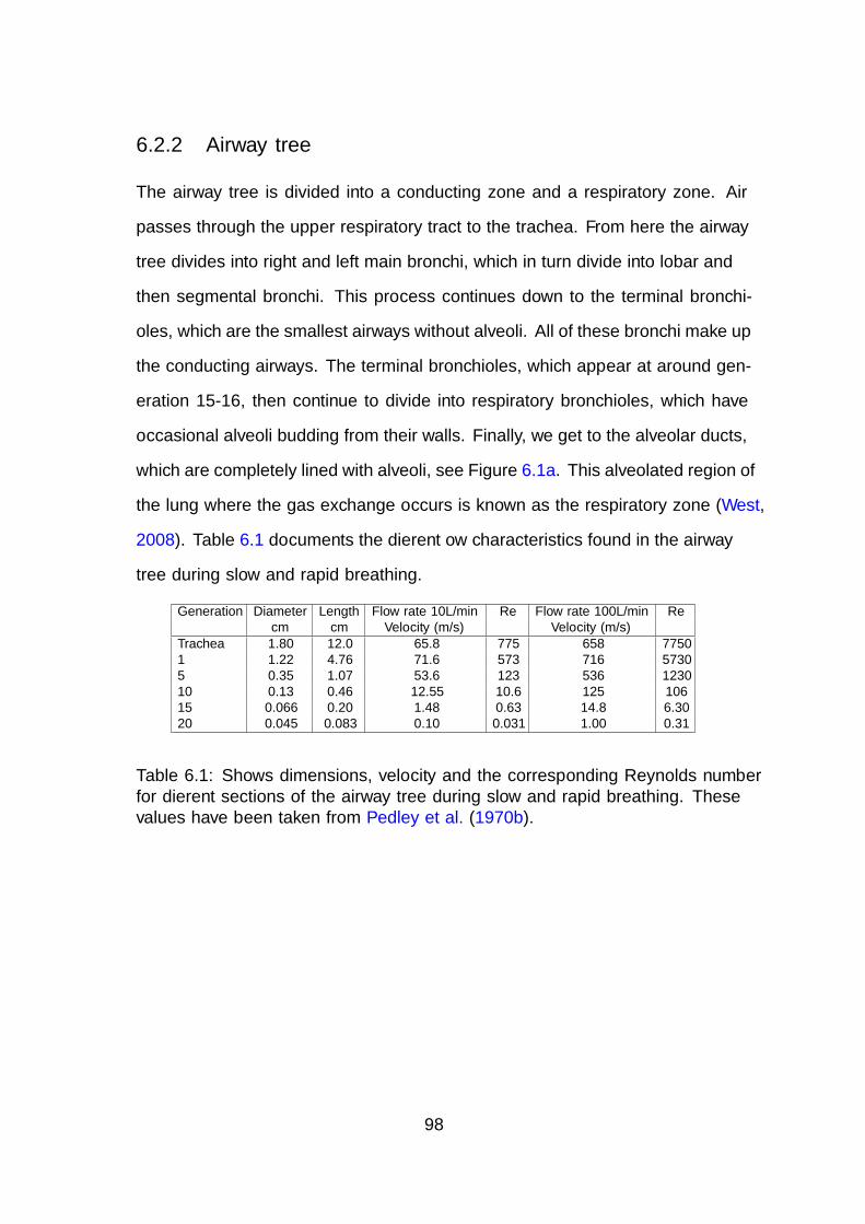
6.2.2 Airway tree

The airway tree is divided into a conducting zone and a respiratory zone. Air

passes through the upper respiratory tract to the trachea. From here the airway

tree divides into right and left main bronchi, which in turn divide into lobar and

then segmental bronchi. This process continues down to the terminal bronchi-

oles, which are the smallest airways without alveoli. All of these bronchi make up

the conducting airways. The terminal bronchioles, which appear at around gen-

eration 15-16, then continue to divide into respiratory bronchioles, which have

occasional alveoli budding from their walls. Finally, we get to the alveolar ducts,

which are completely lined with alveoli, see Figure 6.1a. This alveolated region of

the lung where the gas exchange occurs is known as the respiratory zone (West,

2008). Table 6.1 documents the different flow characteristics found in the airway

tree during slow and rapid breathing.

Generation Diameter Length Flow rate 10L/min Re Flow rate 100L/min Recm cm Velocity (m/s) Velocity (m/s)

Trachea 1.80 12.0 65.8 775 658 77501 1.22 4.76 71.6 573 716 57305 0.35 1.07 53.6 123 536 123010 0.13 0.46 12.55 10.6 125 10615 0.066 0.20 1.48 0.63 14.8 6.3020 0.045 0.083 0.10 0.031 1.00 0.31

Table 6.1: Shows dimensions, velocity and the corresponding Reynolds numberfor different sections of the airway tree during slow and rapid breathing. Thesevalues have been taken from Pedley et al. (1970b).

98

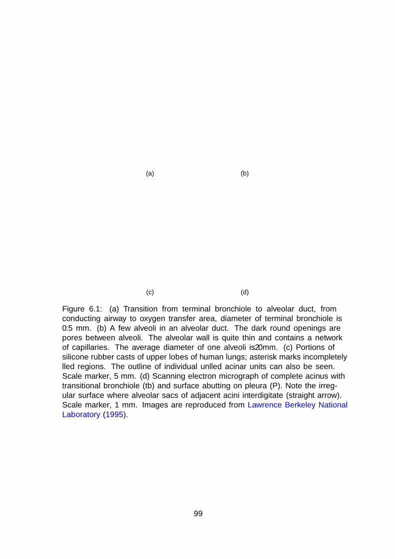
(a) (b)

(c) (d)

Figure 6.1: (a) Transition from terminal bronchiole to alveolar duct, fromconducting airway to oxygen transfer area, diameter of terminal bronchiole is0.5 mm. (b) A few alveoli in an alveolar duct. The dark round openings arepores between alveoli. The alveolar wall is quite thin and contains a networkof capillaries. The average diameter of one alveoli is 0.2 mm. (c) Portions ofsilicone rubber casts of upper lobes of human lungs; asterisk marks incompletelyfilled regions. The outline of individual unfilled acinar units can also be seen.Scale marker, 5 mm. (d) Scanning electron micrograph of complete acinus withtransitional bronchiole (tb) and surface abutting on pleura (P). Note the irreg-ular surface where alveolar sacs of adjacent acini interdigitate (straight arrow).Scale marker, 1 mm. Images are reproduced from Lawrence Berkeley NationalLaboratory (1995).

99

Figure 6.2: A rubber cast of the conducting airways of a human lung. The imageis reproduced from West (2008).

6.2.3 Lung parenchyma

Lung parenchyma refers to the portion of the lung made up of the small air cham-

bers (alveoli) participating in gas exchange. The alveoli are made up of collagen,

elastin fibers and membranous structures containing the capillary network, see

Figure 6.1b. Alveoli are arranged in sponge like structures and fill the entire

volume of the lungs surrounding the conducting passages. Figure 6.1c shows a

rubber cast of lung parenchyma, the dark lines outline the branching structure

of the airways. The right and left lung are partitioned into three and two lobes,

respectively. Lung segments of conic shape are then the first subdivision of these

lobes. These structures are bounded by connective tissue such that surgical sepa-

ration is often possible. In the right lung, there are usually ten segments whereas

only nine can be found in the left lung. Within the segments, the bronchi branch

about six to twelve times. The terminal bronchioles which appear after roughly

15− 16 branching generations then finally feed into approximately 30, 000 acini,

see Figure 6.1d. These acini represent the largest lung units of which all airways

100

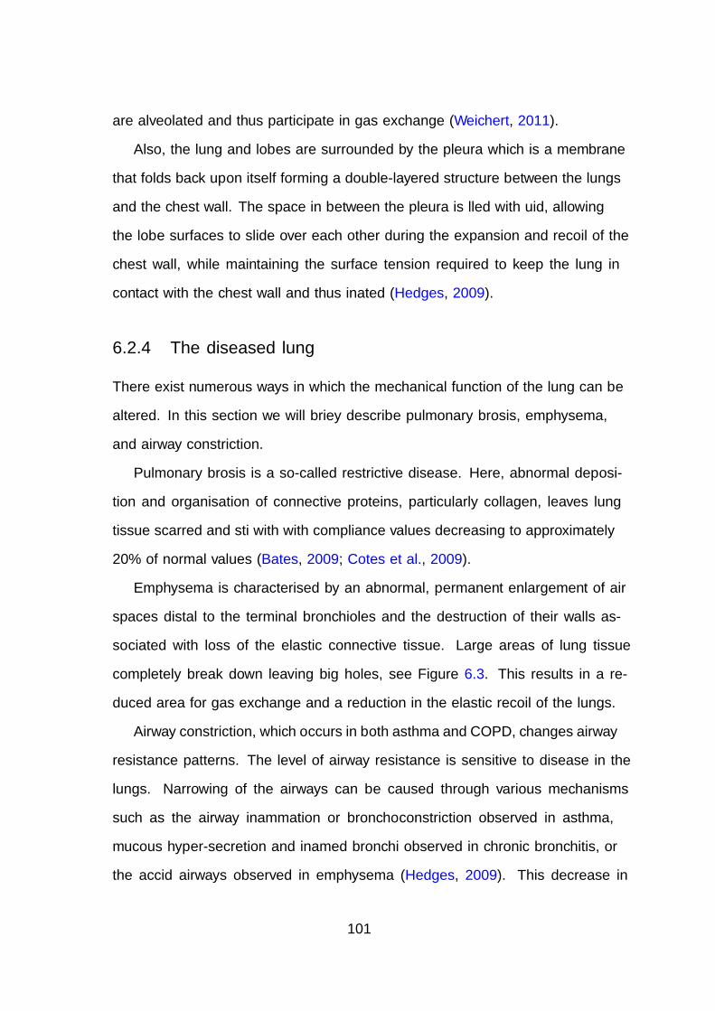
are alveolated and thus participate in gas exchange (Weichert, 2011).

Also, the lung and lobes are surrounded by the pleura which is a membrane

that folds back upon itself forming a double-layered structure between the lungs

and the chest wall. The space in between the pleura is filled with fluid, allowing

the lobe surfaces to slide over each other during the expansion and recoil of the

chest wall, while maintaining the surface tension required to keep the lung in

contact with the chest wall and thus inflated (Hedges, 2009).

6.2.4 The diseased lung

There exist numerous ways in which the mechanical function of the lung can be

altered. In this section we will briefly describe pulmonary fibrosis, emphysema,

and airway constriction.

Pulmonary fibrosis is a so-called restrictive disease. Here, abnormal deposi-

tion and organisation of connective proteins, particularly collagen, leaves lung

tissue scarred and stiff with with compliance values decreasing to approximately

20% of normal values (Bates, 2009; Cotes et al., 2009).

Emphysema is characterised by an abnormal, permanent enlargement of air

spaces distal to the terminal bronchioles and the destruction of their walls as-

sociated with loss of the elastic connective tissue. Large areas of lung tissue

completely break down leaving big holes, see Figure 6.3. This results in a re-

duced area for gas exchange and a reduction in the elastic recoil of the lungs.

Airway constriction, which occurs in both asthma and COPD, changes airway

resistance patterns. The level of airway resistance is sensitive to disease in the

lungs. Narrowing of the airways can be caused through various mechanisms

such as the airway inflammation or bronchoconstriction observed in asthma,

mucous hyper-secretion and inflamed bronchi observed in chronic bronchitis, or

the flaccid airways observed in emphysema (Hedges, 2009). This decrease in

101

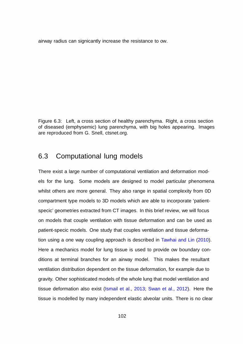
airway radius can significantly increase the resistance to flow.

Figure 6.3: Left, a cross section of healthy parenchyma. Right, a cross sectionof diseased (emphysemic) lung parenchyma, with big holes appearing. Imagesare reproduced from G. Snell, ctsnet.org.

6.3 Computational lung models

There exist a large number of computational ventilation and deformation mod-

els for the lung. Some models are designed to model particular phenomena

whilst others are more general. They also range in spatial complexity from 0D

compartment type models to 3D models which are able to incorporate ‘patient-

specific’ geometries extracted from CT images. In this brief review, we will focus

on models that couple ventilation with tissue deformation and can be used as

patient-specific models. One study that couples ventilation and tissue deforma-

tion using a one way coupling approach is described in Tawhai and Lin (2010).

Here a mechanics model for lung tissue is used to provide flow boundary con-

ditions at terminal branches for an airway model. This makes the resultant

ventilation distribution dependent on the tissue deformation, for example due to

gravity. Other sophisticated models of the whole lung that model ventilation and

tissue deformation also exist (Ismail et al., 2013; Swan et al., 2012). Here the

tissue is modelled by many independent elastic alveolar units. There is no clear

102

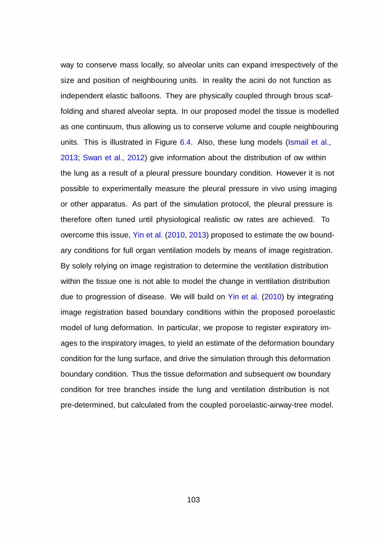
way to conserve mass locally, so alveolar units can expand irrespectively of the

size and position of neighbouring units. In reality the acini do not function as

independent elastic balloons. They are physically coupled through fibrous scaf-

folding and shared alveolar septa. In our proposed model the tissue is modelled

as one continuum, thus allowing us to conserve volume and couple neighbouring

units. This is illustrated in Figure 6.4. Also, these lung models (Ismail et al.,

2013; Swan et al., 2012) give information about the distribution of flow within

the lung as a result of a pleural pressure boundary condition. However it is not

possible to experimentally measure the pleural pressure in vivo using imaging

or other apparatus. As part of the simulation protocol, the pleural pressure is

therefore often tuned until physiological realistic flow rates are achieved. To

overcome this issue, Yin et al. (2010, 2013) proposed to estimate the flow bound-

ary conditions for full organ ventilation models by means of image registration.

By solely relying on image registration to determine the ventilation distribution

within the tissue one is not able to model the change in ventilation distribution

due to progression of disease. We will build on Yin et al. (2010) by integrating

image registration based boundary conditions within the proposed poroelastic

model of lung deformation. In particular, we propose to register expiratory im-

ages to the inspiratory images, to yield an estimate of the deformation boundary

condition for the lung surface, and drive the simulation through this deformation

boundary condition. Thus the tissue deformation and subsequent flow boundary

condition for tree branches inside the lung and ventilation distribution is not

pre-determined, but calculated from the coupled poroelastic-airway-tree model.

103

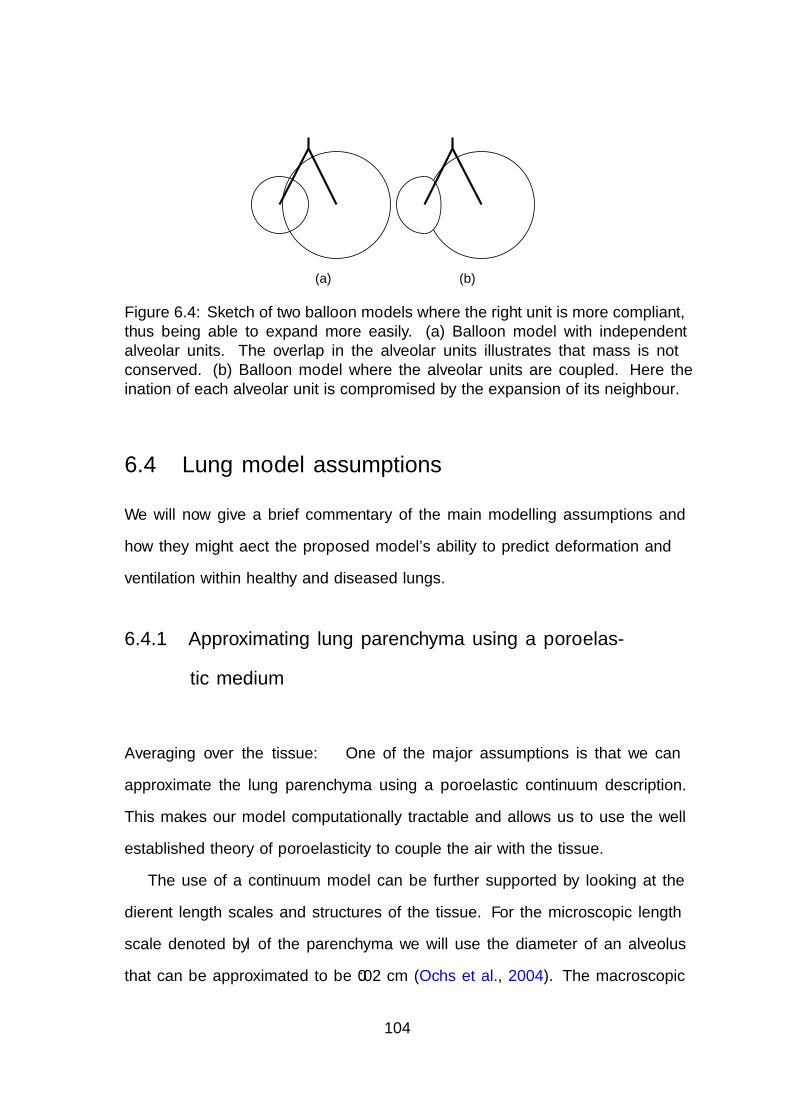
(a) (b)

Figure 6.4: Sketch of two balloon models where the right unit is more compliant,thus being able to expand more easily. (a) Balloon model with independentalveolar units. The overlap in the alveolar units illustrates that mass is notconserved. (b) Balloon model where the alveolar units are coupled. Here theinflation of each alveolar unit is compromised by the expansion of its neighbour.

6.4 Lung model assumptions

We will now give a brief commentary of the main modelling assumptions and

how they might affect the proposed model’s ability to predict deformation and

ventilation within healthy and diseased lungs.

6.4.1 Approximating lung parenchyma using a poroelas-

tic medium

Averaging over the tissue: One of the major assumptions is that we can

approximate the lung parenchyma using a poroelastic continuum description.

This makes our model computationally tractable and allows us to use the well

established theory of poroelasticity to couple the air with the tissue.

The use of a continuum model can be further supported by looking at the

different length scales and structures of the tissue. For the microscopic length

scale denoted by l of the parenchyma we will use the diameter of an alveolus

that can be approximated to be 0.02 cm (Ochs et al., 2004). The macroscopic

104

length scale L can be taken to be the diameter of a segment which measures

around 4 cm of tissue. So the ratio of the different length scales is small i.e

ε := lL≈ 0.005 1. This along with the assumption that the structure of an

acinus is porous (see Figures 6.1b and 6.1a) and approximately periodic supports

the use of averaging techniques over the tissue to obtain a continuum description

in the form of a poroelastic medium. To further simplify the poroelastic equa-

tions we assume that the poroelastic continuum can be described by a solid phase

(blood and tissue) and a fluid phase (air), where both phases are assumed to be

incompressible. The interaction between the fluid pressure and the deformation

of the solid skeleton is assumed to obey the effective stress principle. Note that

by averaging over the tissue we do not seek to model individual alveoli but intro-

duce macroscopic parameters such as the permeability and elasticity coefficients.

In general, lung diseases usually affect significant regions of alveoli (lung tissue),

thus, by changing the macro-scale parameters over the affected area of tissue we

are still able to model changes in the tissue due to disease.

Ignoring blood flow: Apart from collagen, fibers and air the other major

component in the lung is blood. The volume taken up by collagen and elastin

fibers is similar to the volume occupied by the capillaries filled with blood (illus-

trated in Figure 6.1b). In fact, the space not occupied by air is about 7% of the

parenchymal volume and is made up of 50% capillary blood and 50% of collagen

and elastin fibers (Weichert, 2011). Also the density of blood is similar to the

density of tissue and much larger than that of air (1060 kg m−3 1.18 kg m−3).

Since the capillaries are constantly filled with blood and the density of blood is

similar to that of alveolar tissue we will make the simplifying assumption that

the blood is simply part of the tissue (solid phase) and thus ignore accelerations

and any redistribution of blood during breathing.

105

Assuming incompressibility of the solid and the fluid: Blood and tissue

can be assumed to be incompressible. Under physiological conditions, air can

also be assumed to be incompressible (Ismail et al., 2013).

Ignoring solid inertia forces: Simple calculations considering the sinusoidal

motion of tissue near the diaphragm during normal breathing yield an estimate

of 0.02 ms−2 for the maximum acceleration of lung parenchyma. Compared to

the acceleration of gravity this is negligible, and it is therefore reasonable to

ignore the inertia forces in the tissue.

Ignoring fluid inertia forces: The fluid’s Reynolds number in the lower air-

ways that form part of the lung parenchyma, has been estimated to be around

1 to 0.01 (Pedley et al., 1970b). Due to this relatively low Reynolds number we

choose to ignore fluid inertia forces in the poroelastic medium.

Ignoring viscous forces in the fluid: A dimensional analysis shows that the

viscous stress in the fluid is small compared to the drag forces between the fluid

and the porous structure, when the ratio of the different length scales is small

(Markert, 2007). We will therefore neglect the fluid viscous stress implying that

the fluid behaves more or less inviscid within the porous structure.

6.4.2 Approximating the airways using a fluid network

model

In order to make the coupled model computationally feasible we assume that a

simple laminar flow model can describe the air flow in the airways and we make

the common Poiseuille flow assumption. This flow assumption is also made in

106

Leary et al. (2014); Swan et al. (2012) where the air flow in a whole airway

tree, from trachea down to the final bronchioles was assumed to be governed by

Poiseuille flow. Diseases affecting the airway tree can be modelled effectively by

changing resistance (airway radius) parameters in the network flow model.

6.5 Mathematical model

6.5.1 A poroelastic model for lung parenchyma

Having made the assumptions in section 6.4 for the tissue we are left with the

large deformation quasi-static incompressible poroelastic model (2.38).

Constitutive laws.

To close the poroelastic model for the tissue (2.38) we need to choose constitutive

laws for the permeability and strain energy. We will use the same permeability

law that has already been proposed in Kowalczyk and Kleiber (1994) to model

lung parenchyma,

k0 = k0

(Jφ

φ0

)2/3

I. (6.1)

Exponential strain energy laws for lung parenchyma exist, for example the pop-

ular law by Fung (1975). However little is known about how the constants in

these laws should be interpreted and altered to model weakening of the tissue

in an diseased state. Further, the constants in these laws are thought to have

no physical meaning (Tawhai et al., 2009). To make the interpretation of the

elasticity constants and dynamics of the model as simple as possible we chose

a Neo-Hookean law taken from Wriggers (2008), with the penalty term chosen

such that 0 ≤ φ < 1,

W (C) =µ

2(tr(C)− 3) +

λ

4(J2 − 1)− (µ+

λ

2)ln(J − 1 + φ0). (6.2)

107

The material parameters µ and λ can be related to the more familiar Young’s

modulus E and the Poisson ratio ν by µ = E2(1+ν)

and λ = Eν(1+ν)(1−2ν)

. The

values of these constants for modelling lung tissue have been investigated in

De Wilde et al. (1981); Werner et al. (2009); Zhang et al. (2004) and are shown

in Table 6.2.

6.5.2 A network flow model for the airway tree

The flow rate Qi through the ith segment in the airway network is given by the

pressure-flow relationship

Pi,1 − Pi,2 = RiQi, (6.3)

where Ri =8lµfπr4

is the Poiseuille flow resistance of a pipe segment, where r

and l are the radius and length of the pipe, µf is the dynamic viscosity, and Pi,1

and Pi,2 are the pressures at the proximal and distal nodes of the pipe segment,

respectively. Let Ai be the set of pipe segments emanating from the ith pipe

segment in the airway network. We can express the conservation of flow in the

airway network as

Qi =∑j∈Ai

Qj. (6.4)

The outlet pressure of the airway network is set using the boundary condition

P0 = P .

Coupling the airway network to the poroelastic model.

We introduce subdomains to identify the region of the domain that is supplied

with fluid from a specific branch of the airway network and returns fluid through

that branch. For notational purposes we use the subscript di to indicate the

most distal branches that have no further conducting branches emanating from

108

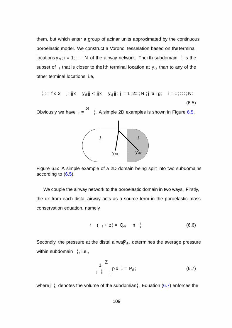
them, but which enter a group of acinar units approximated by the continuous

poroelastic model. We construct a Voronoi tesselation based on the N terminal

locations ydi, i = 1, . . . , N of the airway network. The ith subdomain Ωit is the

subset of Ωt that is closer to the ith terminal location at ydi than to any of the

other terminal locations, i.e,

Ωit := x ∈ Ωt : ||x− ydi|| < ||x− ydj||, j = 1, 2..., N , j 6= i , i = 1, . . . , N.

(6.5)

Obviously we have Ωt =⋃

Ωit. A simple 2D examples is shown in Figure 6.5.

yd2

Ω2t

yd1

Ω1t

Figure 6.5: A simple example of a 2D domain being split into two subdomainsaccording to (6.5).

We couple the airway network to the poroelastic domain in two ways. Firstly,

the flux from each distal airway acts as a source term in the poroelastic mass

conservation equation, namely

∇ · (χt + z) = Qdi in Ωit. (6.6)

Secondly, the pressure at the distal airway Pdi, determines the average pressure

within subdomain Ωit, i.e.,

1

|Ωit|

∫Ωit

p dΩit = Pdi, (6.7)

where |Ωit| denotes the volume of the subdomian Ωi

t. Equation (6.7) enforces the

109

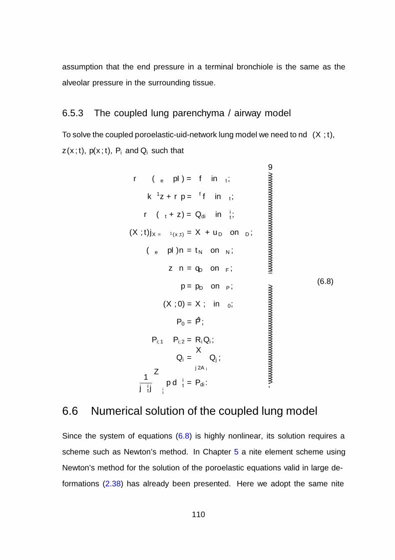
assumption that the end pressure in a terminal bronchiole is the same as the

alveolar pressure in the surrounding tissue.

6.5.3 The coupled lung parenchyma / airway model

To solve the coupled poroelastic-fluid-network lung model we need to find χ(X, t),

z(x, t), p(x, t), Pi and Qi such that

−∇ · (σe − pI) = ρf in Ωt,

k−1z +∇p = ρff in Ωt,

∇ · (χt + z) = Qdi in Ωit,

χ(X, t)|X=χ−1(x,t) = X + uD on ΓD,

(σe − pI)n = tN on ΓN ,

z · n = qD on ΓF ,

p = pD on ΓP ,

χ(X, 0) = X, in Ω0,

P0 = P ,

Pi,1 − Pi,2 = RiQi,

Qi =∑j∈Ai

Qj,

1

|Ωit|

∫Ωit

p dΩit = Pdi.

(6.8)

6.6 Numerical solution of the coupled lung model

Since the system of equations (6.8) is highly nonlinear, its solution requires a

scheme such as Newton’s method. In Chapter 5 a finite element scheme using

Newton’s method for the solution of the poroelastic equations valid in large de-

formations (2.38) has already been presented. Here we adopt the same finite

110

element scheme as presented in Chapter 5 for solving the poroelastic equations

and expand the linear system (discretised linearisation) to include additional

matrices required for solving the fluid network and its coupling to the poroe-

lastic medium. This results in a monolithic coupling scheme that ensures good

convergence even for problems with strong coupling interactions between the

poroelastic medium and the fluid network. In section 6.6.1 we describe how to

couple the fluid network to the discrete poroelastic model, and in section 6.6.2

we present details on how the stiffness matrix K (discretised linearisation of the

full lung model (6.8)), and the residual vector R are built.

6.6.1 Discrete coupling of the fluid network to the poroe-

lastic model

If we discretise the space using triangles and employ a piecewise constant pressure

approximation (one node at the center of each element), the resulting coupling

for the simple 2D example (Figure 6.5) is shown in Figure 6.6a. Once we refine

the mesh (Figure 6.6b), the discretised division of subdomains tends to the sub-

division of the original problem (Figure 6.5). The ith discretised subdomain Ωit

is defined as the set of elements Ek whose centroids xk are closer to the distal end

of the ith terminal branch than to the distal end of any other terminal branch,

i.e.,

Ωit := Ek ∈ Ωt : ||xk − ydi|| < ||xk − ydj||, j = 1, 2..., N , j 6= i . (6.9)

111

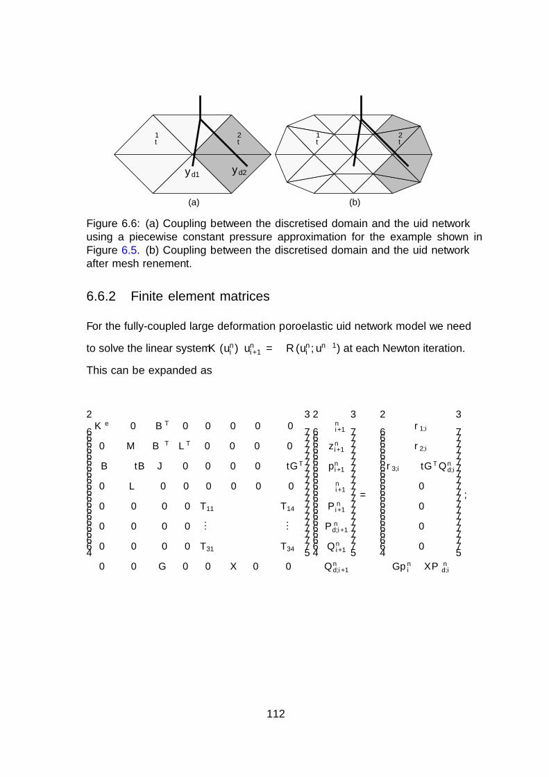
yd2

Ω2t

yd1

Ω1t

(a)

Ω2tΩ1

t

(b)

Figure 6.6: (a) Coupling between the discretised domain and the fluid networkusing a piecewise constant pressure approximation for the example shown inFigure 6.5. (b) Coupling between the discretised domain and the fluid networkafter mesh refinement.

6.6.2 Finite element matrices

For the fully-coupled large deformation poroelastic fluid network model we need

to solve the linear system K(uni )ξuni+1 = −R(uni , un−1) at each Newton iteration.

This can be expanded as

Ke 0 BT 0 0 0 0 0

0 M BT LT 0 0 0 0

−B −∆tB J 0 0 0 0 −∆tGT

0 L 0 0 0 0 0 0

0 0 0 0 T11 · · · · · · T14

0 0 0 0...

...

0 0 0 0 T31 · · · · · · T34

0 0 G 0 0 −X 0 0

ξχni+1

ξzni+1

ξpni+1

ξΛni+1

ξP ni+1

ξP nd,i+1

ξQni+1

ξQnd,i+1

= −

r1,i

r2,i

r3,i −∆tGTQnd,i

0

0

0

0

Gpni −XP nd,i

,

112

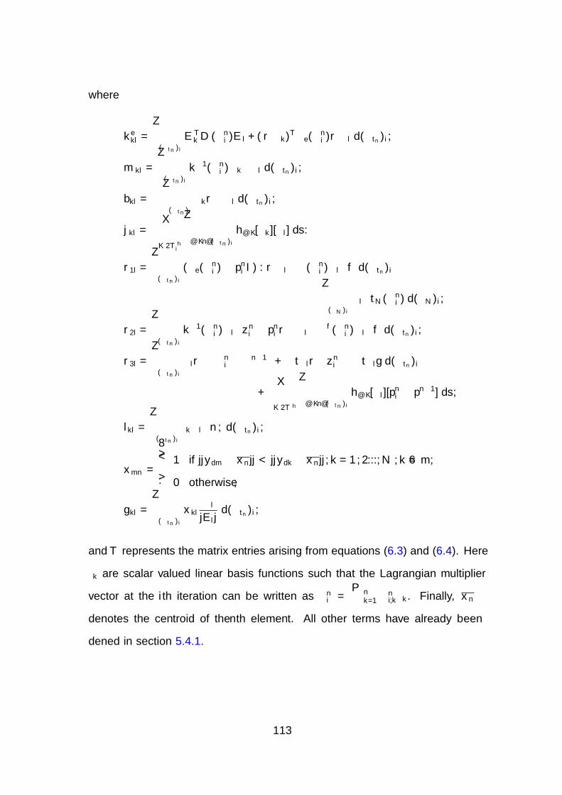
where

kekl =

∫(Ωtn )i

ETkD(χni )El + (∇φk)Tσe(χni )∇φl d(Ωtn)i,

mkl =

∫(Ωtn )i

k−1(χni )φk · φl d(Ωtn)i,

bkl = −∫

(Ωtn )i

ψk∇ · φl d(Ωtn)i,

jkl = δ∑K∈T hi

∫∂K\∂(Ωtn )i

h∂K [ψk][ψl] ds.

r1l =

∫(Ωtn )i

(σe(χni )− pni I) : ∇φl − ρ(χni )φl · f d(Ωtn)i

−∫

(ΓN )i

φl · tN(χni ) d(ΓN)i,

r2l =

∫(Ωtn )i

k−1(χni )φl · zni − pni∇ · φl − ρf (χni )φl · f d(Ωtn)i,

r3l =

∫(Ωtn )i

ψl∇ ·(χni − χn−1

)+ ∆tψl∇ · zni −∆tψlg d(Ωtn)i

+δ∑K∈T h

∫∂K\∂(Ωtn )i

h∂K [ψl][pni − pn−1] ds,

lkl =

∫(Ωtn )i

εkφl · n, d(Ωtn)i,

xmn =

1 if ||ydm − xn|| < ||ydk − xn||, k = 1, 2..., N , k 6= m,

0 otherwise,

gkl =

∫(Ωtn )i

xklφl|El|

d(Ωtn)i,

and T represents the matrix entries arising from equations (6.3) and (6.4). Here

εk are scalar valued linear basis functions such that the Lagrangian multiplier

vector at the ith iteration can be written as Λni =

∑nΛ

k=1 Λni,kεk. Finally, xn

denotes the centroid of the nth element. All other terms have already been

defined in section 5.4.1.

113

6.7 Model generation

6.7.1 Mesh generation

We derive a whole organ lung model, of the right lung, from a high-resolution CT

image taken at total lung capacity (TLC) and functional residual capacity (FRC).

The bulk lung is first segmented from the CT data (slice thickness and pixel size

0.73 mm) using the commercially available segmentation software Mimics1. We

then use the open-source image processing toolbox iso2mesh (Fang and Boas,

2009) to generate a Tetrahedral mesh containing 38369 elements. The conducting

airways are also segmented from the CT data taken at TLC level, and a centerline

with radial information is calculated. To approximate the remaining airways up

to generation 8-13 we use a volume filling airway generation algorithm to generate

a mesh of the airway tree containing 13696 nodes, with 2140 terminal branches

(Bordas et al., 2014).

6.7.2 Reference state, boundary conditions and initial con-

ditions

The poroelastic framework we have described requires a stress free reference state.

However biological tissues do not possess a ‘reference state’ in space where the

material is free of both stress and strain. The cells that make up tissues are born

into stressed states and live out their lives in these stressed states (Freed and

Einstein, 2013).

In this work, we scale the lung from FRC to a configuration, the reference

state, in which the internal stresses and strains are assumed to be zero. The

geometry of the reference state is then used as the initial configuration of the

lung model. The lung model is then uniformly inflated from the reference state

1http://biomedical.materialise.com/mimics

114

to create a pre-stressed FRC configuration which has a mean elastic recoil of

about 0.49 × 103 Pa, commonly understood to be a typical value (West, 2008).

From there we simulate tidal breathing. A similar approach has also been used

in Lee et al. (1983).

We register the expiratory (FRC) segmentation to the segmentation at TLC

using a simple registration procedure that uses three scalings in the x, y and

z direction to map between the bounding boxes of the segmentations at FRC

and TLC. This yields a rough estimate of the deformation field for the lung

surface from expiration to inspiration. To simulate tidal breathing we assume a

sinusoidal breathing cycle and expand the lung surface from FRC to 40% of the

deformation from FRC to TLC,

uD(·, t) = 0.2

(1 + sin

(tπ

2+

3π

2

))uD,TLC on Γd. (6.10)

Here uD,TLC is the deformation of the lung surface from FRC to TLC, obtained

using the registration procedure. For our mesh and registration this results in a

physiologically realistic tidal volume of 0.59 liters. We simulate breathing for a

total of 8 seconds (2 breathing cycles) resulting in a breathing frequency of 15

breaths per minute. Due to the incompressibility of the poroelastic tissue this

also determines the total volume of air inspired/expired and the flowrate at the

trachea, see Figure 6.8a and 6.8b respectively. For the fluid boundary condition

we have that the whole lung is sealed so that no fluid can escape through the lung

surface (except via the trachea), with z · n = 0 along the whole boundary. For

the airway network boundary condition we set the outlet pressure of the airway

network to zero atmospheric pressure, P0 = 0.

115

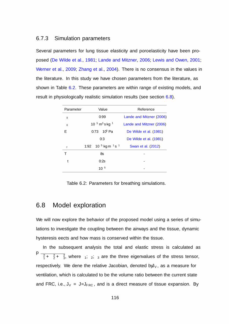
6.7.3 Simulation parameters

Several parameters for lung tissue elasticity and poroelasticity have been pro-

posed (De Wilde et al., 1981; Lande and Mitzner, 2006; Lewis and Owen, 2001;

Werner et al., 2009; Zhang et al., 2004). There is no consensus in the values in

the literature. In this study we have chosen parameters from the literature, as

shown in Table 6.2. These parameters are within range of existing models, and

result in physiologically realistic simulation results (see section 6.8).

Parameter Value Reference

φ0 0.99 Lande and Mitzner (2006)

κ0 10−5 m3 s kg−1 Lande and Mitzner (2006)

E 0.73× 103 Pa De Wilde et al. (1981)

ν 0.3 De Wilde et al. (1981)

µf 1.92× 10−5 kg m−1 s−1 Swan et al. (2012)

T 8s -

∆t 0.2s -

δ 10−5 -

Table 6.2: Parameters for breathing simulations.

6.8 Model exploration

We will now explore the behavior of the proposed model using a series of simu-

lations to investigate the coupling between the airways and the tissue, dynamic

hysteresis effects and how mass is conserved within the tissue.

In the subsequent analysis the total and elastic stress is calculated as√λ2

1 + λ22 + λ2

3, where λ1, λ2, λ3 are the three eigenvalues of the stress tensor,

respectively. We define the relative Jacobian, denoted by JV , as a measure for

ventilation, which is calculated to be the volume ratio between the current state

and FRC, i.e., JV = J/JFRC , and is a direct measure of tissue expansion. By

116

running simulations over many breaths we have found that differences between

the second breath and subsequent breaths were negligible, and therefore only

results from the second breath, t = 4s to t = 8s are presented. The sagital slice

shown in Figure 6.7a gives a good representation of the general dynamics within

the tissue. Unless otherwise stated, all subsequent figures that do not show time

courses are taken at t = 5.8s just before peak inhalation of the second time

breath in the simulation.

To solve the nonlinear poroelastic problem using Newton’s method at a par-

ticular time step, we perform the the steps already described in algorithm 2.

We set the relative tolerance to be TOL = 10−4. For the subsequent numerical

results, a maximum of 5 Newton iterations were required to solve each time step.

(a) (b)

Figure 6.7: (a) The blue sagital slice indicates the position of subsequent slicesused for the data analysis of the tissue. (b) The red ball represents the struc-turally modified region, used to prescribe airway constriction and tissue weaken-ing.

117

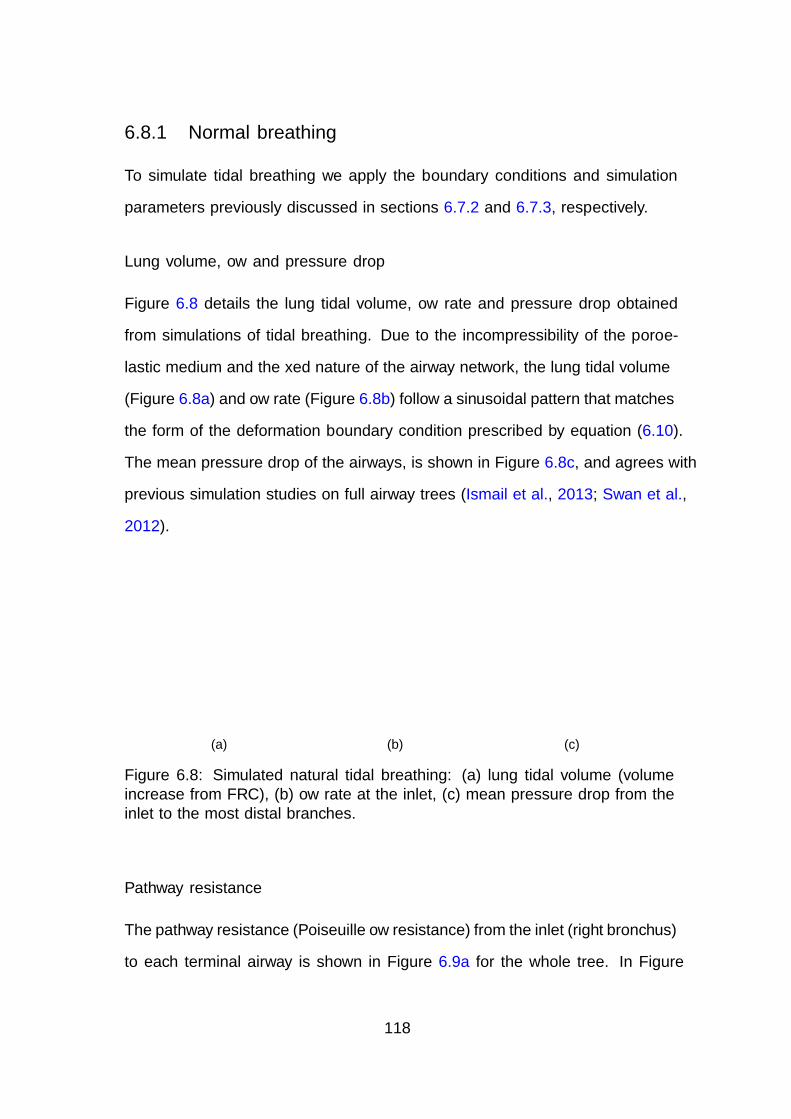
6.8.1 Normal breathing

To simulate tidal breathing we apply the boundary conditions and simulation

parameters previously discussed in sections 6.7.2 and 6.7.3, respectively.

Lung volume, flow and pressure drop

Figure 6.8 details the lung tidal volume, flow rate and pressure drop obtained

from simulations of tidal breathing. Due to the incompressibility of the poroe-

lastic medium and the fixed nature of the airway network, the lung tidal volume

(Figure 6.8a) and flow rate (Figure 6.8b) follow a sinusoidal pattern that matches

the form of the deformation boundary condition prescribed by equation (6.10).

The mean pressure drop of the airways, is shown in Figure 6.8c, and agrees with

previous simulation studies on full airway trees (Ismail et al., 2013; Swan et al.,

2012).

4 4.5 5 5.5 6 6.5 7 7.5 80

0.1

0.2

0.3

0.4

0.5

0.6

Volume(L

)

time (s)

(a)

4 5 6 7 8−0.5

−0.25

0

0.25

0.5

Flow

rate

(L/s)

time (s)

(b)

4 5 6 7 8−50

−25

0

25

50

Meanpressure

drop(P

a)

time (s)

(c)

Figure 6.8: Simulated natural tidal breathing: (a) lung tidal volume (volumeincrease from FRC), (b) flow rate at the inlet, (c) mean pressure drop from theinlet to the most distal branches.

Pathway resistance

The pathway resistance (Poiseuille flow resistance) from the inlet (right bronchus)

to each terminal airway is shown in Figure 6.9a for the whole tree. In Figure

118

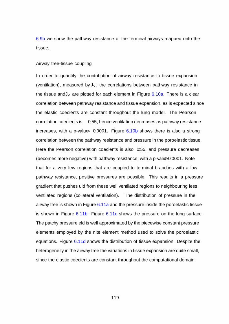
6.9b we show the pathway resistance of the terminal airways mapped onto the

tissue.

Airway tree-tissue coupling

In order to quantify the contribution of airway resistance to tissue expansion

(ventilation), measured by JV , the correlations between pathway resistance in

the tissue and JV are plotted for each element in Figure 6.10a. There is a clear

correlation between pathway resistance and tissue expansion, as is expected since

the elastic coefficients are constant throughout the lung model. The Pearson

correlation coefficients is−0.55, hence ventilation decreases as pathway resistance

increases, with a p-value < 0.0001. Figure 6.10b shows there is also a strong

correlation between the pathway resistance and pressure in the poroelastic tissue.

Here the Pearson correlation coefficients is also −0.55, and pressure decreases

(becomes more negative) with pathway resistance, with a p-value < 0.0001. Note

that for a very few regions that are coupled to terminal branches with a low

pathway resistance, positive pressures are possible. This results in a pressure

gradient that pushes fluid from these well ventilated regions to neighbouring less

ventilated regions (collateral ventilation). The distribution of pressure in the

airway tree is shown in Figure 6.11a and the pressure inside the poroelastic tissue

is shown in Figure 6.11b. Figure 6.11c shows the pressure on the lung surface.

The patchy pressure field is well approximated by the piecewise constant pressure

elements employed by the finite element method used to solve the poroelastic

equations. Figure 6.11d shows the distribution of tissue expansion. Despite the

heterogeneity in the airway tree the variations in tissue expansion are quite small,

since the elastic coefficients are constant throughout the computational domain.

119

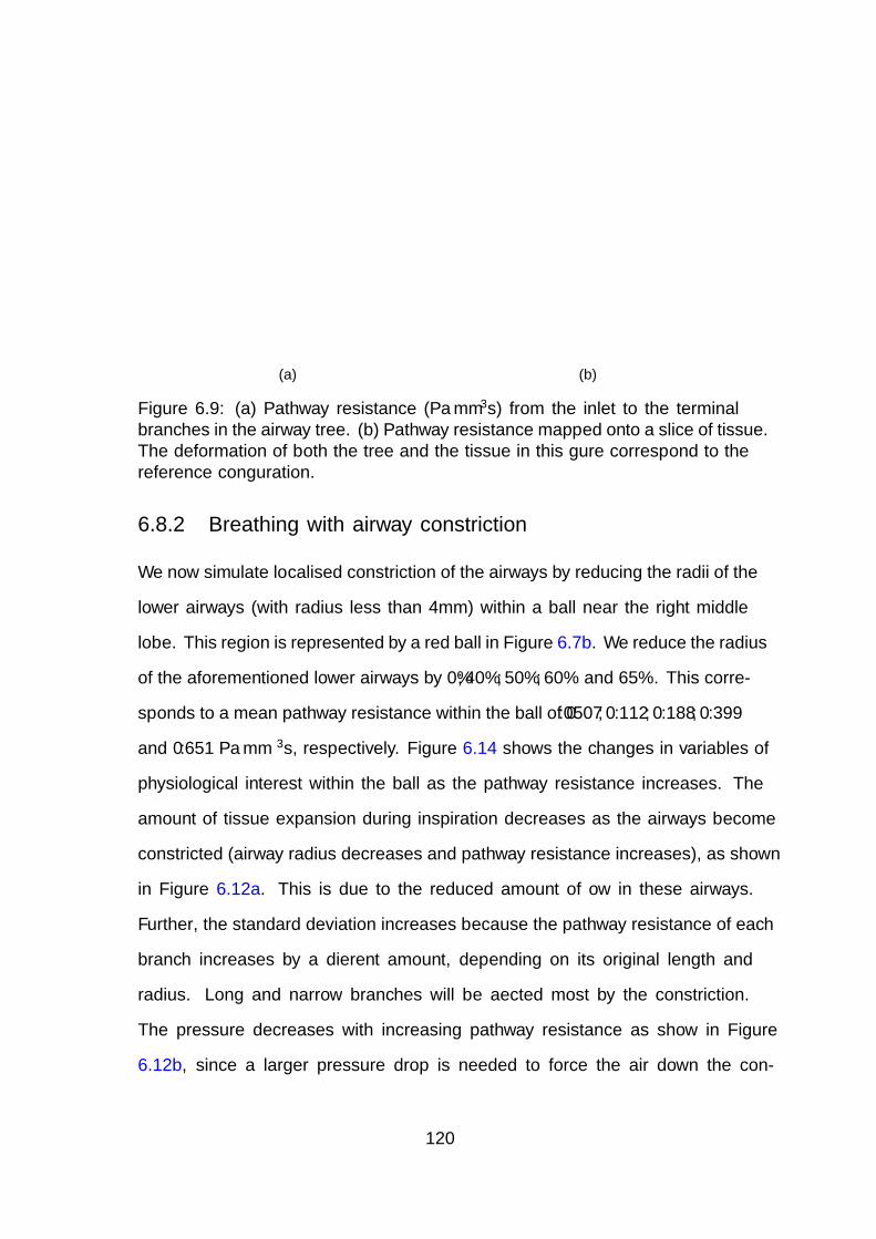
(a) (b)

Figure 6.9: (a) Pathway resistance (Pa mm−3s) from the inlet to the terminalbranches in the airway tree. (b) Pathway resistance mapped onto a slice of tissue.The deformation of both the tree and the tissue in this figure correspond to thereference configuration.

6.8.2 Breathing with airway constriction

We now simulate localised constriction of the airways by reducing the radii of the

lower airways (with radius less than 4mm) within a ball near the right middle

lobe. This region is represented by a red ball in Figure 6.7b. We reduce the radius

of the aforementioned lower airways by 0%, 40%, 50%, 60% and 65%. This corre-

sponds to a mean pathway resistance within the ball of 0.0507, 0.112, 0.188, 0.399

and 0.651 Pa mm−3s, respectively. Figure 6.14 shows the changes in variables of

physiological interest within the ball as the pathway resistance increases. The

amount of tissue expansion during inspiration decreases as the airways become

constricted (airway radius decreases and pathway resistance increases), as shown

in Figure 6.12a. This is due to the reduced amount of flow in these airways.

Further, the standard deviation increases because the pathway resistance of each

branch increases by a different amount, depending on its original length and

radius. Long and narrow branches will be affected most by the constriction.

The pressure decreases with increasing pathway resistance as show in Figure

6.12b, since a larger pressure drop is needed to force the air down the con-

120

0 0.05 0.1 0.15 0.2

1.13

1.14

1.15

1.16

1.17

1.18

JV

Pathway resistance (Pamm−3 s)

(a)

0 0.05 0.1 0.15 0.2

−200

−150

−100

−50

0

Pressure

(Pa)

Pathway resistance (Pamm−3 s)

(b)

Figure 6.10: (a) Correlation between tissue expansion (ventilation) and resistanceof the pathways from the inlet to the terminal branch. (b) Correlation betweenpressure in the poroelastic medium (alveolar pressure) and pathway resistance.

stricted branches. Figure 6.12c shows the elastic stress in the tissue decreases as

pathway resistance increases due to the decrease in tissue deformation (strain).

However, as seen in Figure 6.13c, a large elastic stress appears near the boundary

of the constricted region where the tissue is expanded by the surrounding tissue.

The simulations results shown in Figure 6.13 were performed with 65% airway

constriction in the lower airways, applied within the structurally modified region.

The volume conserving property (mass conservation) of the method is illustrated

in Figure 6.13b where the tissue surrounding the constricted area is expanding to

compensate for the reduction of tissue expansion due to the constriction within

the structurally modified region. Figure 6.13a shows an increase in pressure

near the boundary of this region. This facilitates a pressure gradient that allows

for air to flow into the constricted region (collateral ventilation) to partially

compensate for the reduced amount of ventilation, as is shown in Figure 6.13d.

The magnitude of the maximum flow within the tissue is 8× 10−4 ms−1, this is

quite small and is due to the low permeability applied homogeneously within the

model.

121

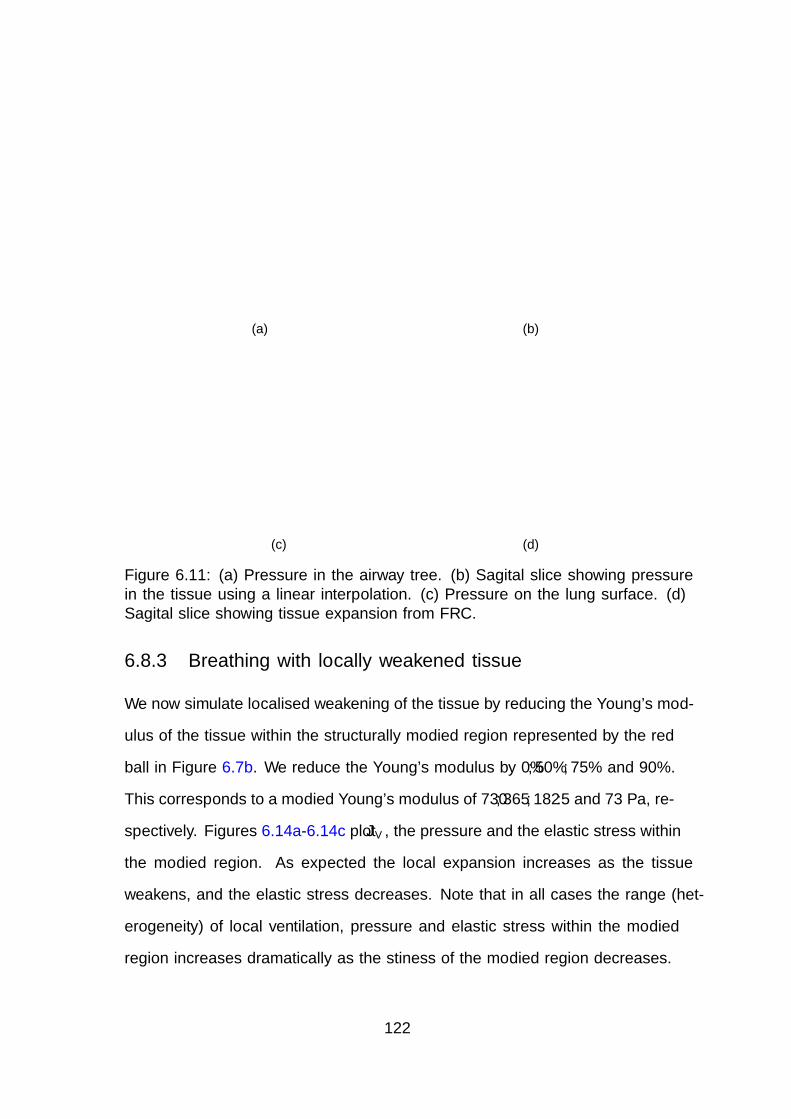
(a) (b)

(c) (d)

Figure 6.11: (a) Pressure in the airway tree. (b) Sagital slice showing pressurein the tissue using a linear interpolation. (c) Pressure on the lung surface. (d)Sagital slice showing tissue expansion from FRC.

6.8.3 Breathing with locally weakened tissue

We now simulate localised weakening of the tissue by reducing the Young’s mod-

ulus of the tissue within the structurally modified region represented by the red

ball in Figure 6.7b. We reduce the Young’s modulus by 0%, 50%, 75% and 90%.

This corresponds to a modified Young’s modulus of 730, 365, 182.5 and 73 Pa, re-

spectively. Figures 6.14a-6.14c plot JV , the pressure and the elastic stress within

the modified region. As expected the local expansion increases as the tissue

weakens, and the elastic stress decreases. Note that in all cases the range (het-

erogeneity) of local ventilation, pressure and elastic stress within the modified

region increases dramatically as the stiffness of the modified region decreases.

122

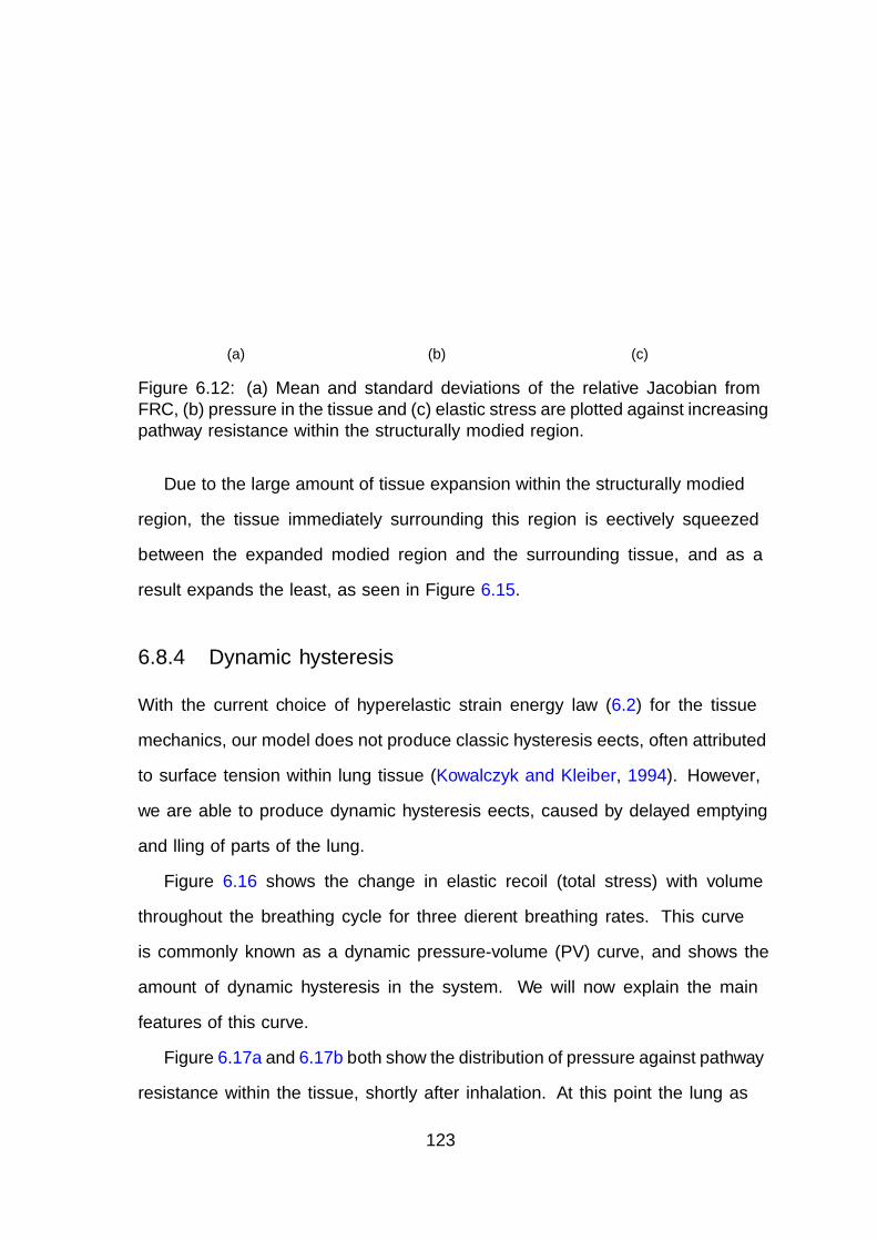
0 0.2 0.4 0.6

1.05

1.1

1.15

1.2

JV

Pathway resistance (Pamm−3 s)

(a)

0 0.2 0.4 0.6

−150

−100

−50

0

Pressure

(Pa)

Pathway resistance (Pamm−3 s)

(b)

0 0.2 0.4 0.6

550

600

650

700

750

Elastic

stress

(Pa)

Pathway resistance (Pamm−3 s)

(c)

Figure 6.12: (a) Mean and standard deviations of the relative Jacobian fromFRC, (b) pressure in the tissue and (c) elastic stress are plotted against increasingpathway resistance within the structurally modified region.

Due to the large amount of tissue expansion within the structurally modified

region, the tissue immediately surrounding this region is effectively squeezed

between the expanded modified region and the surrounding tissue, and as a

result expands the least, as seen in Figure 6.15.

6.8.4 Dynamic hysteresis

With the current choice of hyperelastic strain energy law (6.2) for the tissue

mechanics, our model does not produce classic hysteresis effects, often attributed

to surface tension within lung tissue (Kowalczyk and Kleiber, 1994). However,

we are able to produce dynamic hysteresis effects, caused by delayed emptying

and filling of parts of the lung.

Figure 6.16 shows the change in elastic recoil (total stress) with volume

throughout the breathing cycle for three different breathing rates. This curve

is commonly known as a dynamic pressure-volume (PV) curve, and shows the

amount of dynamic hysteresis in the system. We will now explain the main

features of this curve.

Figure 6.17a and 6.17b both show the distribution of pressure against pathway

resistance within the tissue, shortly after inhalation. At this point the lung as

123

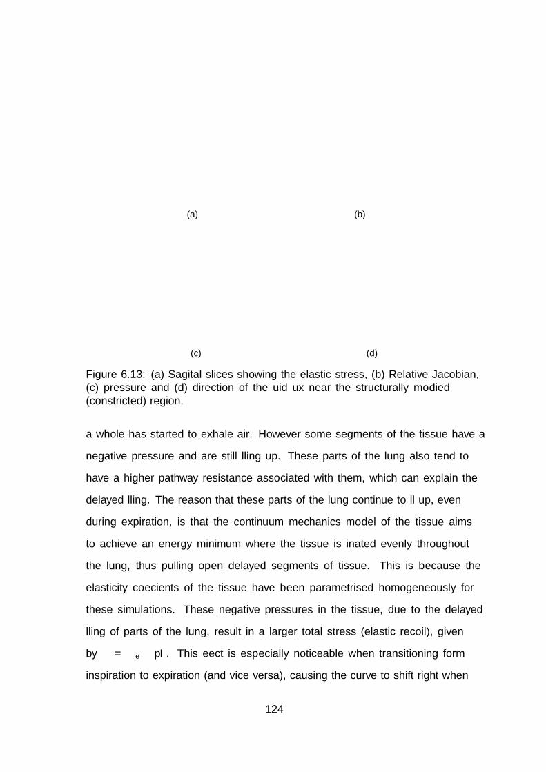
(a) (b)

(c) (d)

Figure 6.13: (a) Sagital slices showing the elastic stress, (b) Relative Jacobian,(c) pressure and (d) direction of the fluid flux near the structurally modified(constricted) region.

a whole has started to exhale air. However some segments of the tissue have a

negative pressure and are still filling up. These parts of the lung also tend to

have a higher pathway resistance associated with them, which can explain the

delayed filling. The reason that these parts of the lung continue to fill up, even

during expiration, is that the continuum mechanics model of the tissue aims

to achieve an energy minimum where the tissue is inflated evenly throughout

the lung, thus pulling open delayed segments of tissue. This is because the

elasticity coefficients of the tissue have been parametrised homogeneously for

these simulations. These negative pressures in the tissue, due to the delayed

filling of parts of the lung, result in a larger total stress (elastic recoil), given

by σ = σe − pI. This effect is especially noticeable when transitioning form

inspiration to expiration (and vice versa), causing the curve to shift right when

124

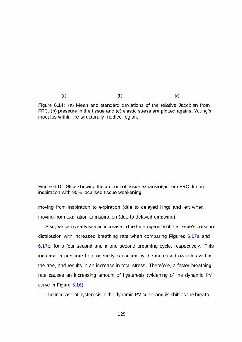
02004006008001

1.2

1.4

1.6

1.8

2

2.2

2.4JV

Young’s modulus (Pa)

(a)

0200400600800

−125

−100

−75

−50

−25

0

Pressure

(Pa)

Young’s modulus (Pa)

(b)

0200400600800

200

400

600

800

Elastic

stress

(Pa)

Young’s modulus (Pa)

(c)

Figure 6.14: (a) Mean and standard deviations of the relative Jacobian fromFRC, (b) pressure in the tissue and (c) elastic stress are plotted against Young’smodulus within the structurally modified region.

Figure 6.15: Slice showing the amount of tissue expansion (JV ) from FRC duringinspiration with 90% localised tissue weakening.

moving from inspiration to expiration (due to delayed filling) and left when

moving from expiration to inspiration (due to delayed emptying).

Also, we can clearly see an increase in the heterogeneity of the tissue’s pressure

distribution with increased breathing rate when comparing Figures 6.17a and

6.17b, for a four second and a one second breathing cycle, respectively. This

increase in pressure heterogeneity is caused by the increased flow rates within

the tree, and results in an increase in total stress. Therefore, a faster breathing

rate causes an increasing amount of hysteresis (widening of the dynamic PV

curve in Figure 6.16).

The increase of hysteresis in the dynamic PV curve and its shift as the breath-

125

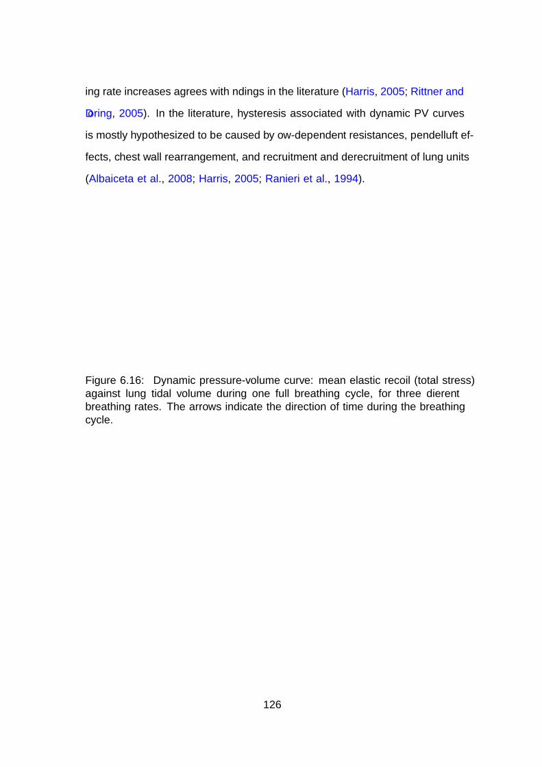
ing rate increases agrees with findings in the literature (Harris, 2005; Rittner and

Doring, 2005). In the literature, hysteresis associated with dynamic PV curves

is mostly hypothesized to be caused by flow-dependent resistances, pendelluft ef-

fects, chest wall rearrangement, and recruitment and derecruitment of lung units

(Albaiceta et al., 2008; Harris, 2005; Ranieri et al., 1994).

400 600 800 10000

0.1

0.2

0.3

0.4

0.5

0.6

Volume(L

)

Mean elastic recoil (Pa)

1s breathing cycle4s breathing cycle16s breathing cycle

Figure 6.16: Dynamic pressure-volume curve: mean elastic recoil (total stress)against lung tidal volume during one full breathing cycle, for three differentbreathing rates. The arrows indicate the direction of time during the breathingcycle.

126

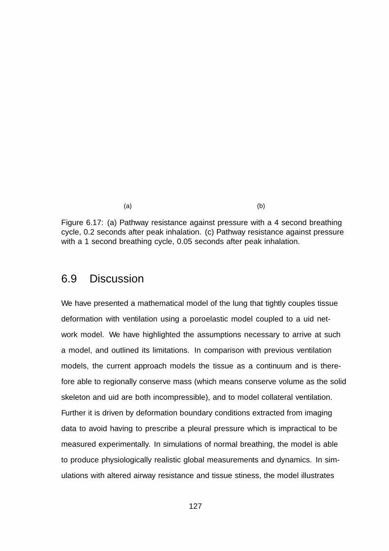
0 0.05 0.1 0.15 0.2

−200

−150

−100

−50

0

50Pressure

(Pa)

Pathway resistance (Pamm−3 s)

4 second breathing cycle

(a)

0 0.05 0.1 0.15 0.2

−200

−150

−100

−50

0

50

Pressure

(Pa)

Pathway resistance (Pamm−3 s)

1 second breathing cycle

(b)

Figure 6.17: (a) Pathway resistance against pressure with a 4 second breathingcycle, 0.2 seconds after peak inhalation. (c) Pathway resistance against pressurewith a 1 second breathing cycle, 0.05 seconds after peak inhalation.

6.9 Discussion

We have presented a mathematical model of the lung that tightly couples tissue

deformation with ventilation using a poroelastic model coupled to a fluid net-

work model. We have highlighted the assumptions necessary to arrive at such

a model, and outlined its limitations. In comparison with previous ventilation

models, the current approach models the tissue as a continuum and is there-

fore able to regionally conserve mass (which means conserve volume as the solid

skeleton and fluid are both incompressible), and to model collateral ventilation.

Further it is driven by deformation boundary conditions extracted from imaging

data to avoid having to prescribe a pleural pressure which is impractical to be

measured experimentally. In simulations of normal breathing, the model is able

to produce physiologically realistic global measurements and dynamics. In sim-

ulations with altered airway resistance and tissue stiffness, the model illustrates

127

the interdependence of the tissue and airway mechanics and thus the importance

of a fully coupled model.

6.9.1 Contributors of airway resistance and tissue me-

chanics to lung function

We have found that there is a strong correlation between airway resistance and

ventilation, see Figure 6.10a. Also, due to heterogeneity in airway resistance,

hysteresis effects appear during breathing (Figure 6.16) and result in a complex

ventilation distribution, caused by delayed filling and emptying of the tissue. Due

to the Poiseuille law that governs the flow through the airways, small changes in

airway radii can result in large changes in pathway resistance, which in turn can

significantly affect the results of the coupled model. Thus, parameterising the

airways correctly is very important. However this is notoriously difficult since CT

data is only available down to the 5-6th generation, and small errors and biases in

the segmentation, that get propagated by the airway generation algorithm, can

have large influences in determining the simulation results. Changes in tissue

elasticity coefficients also play an important role in determining the function

of the lung model. This has been demonstrated in section 6.8.3 where are a

reduction in the Young’s modulus within a specified region causes significant

changes in ventilation, pressure and stress.

6.9.2 Limitations and future work

In order to move towards a more realistic model of the lung breathing, many

steps need to be taken. We will list the main limitations that exist in the airway

tree model, the poroelastic model, the boundary conditions and the geometry,

and give indications on how these could be addressed in a future model.

128

Airway tree limitations: (1) The airway tree flow model currently imple-

mented makes the Poiseuille flow assumption for the whole tree. The Poiseuille

flow assumption requires flow to be fully developed and laminar. This may be

true for the smaller airways where the Reynolds number is small but is certainly

false for the larger upper airways where high Reynolds number flows occur. Such

a model will therefore not be able to capture the high Reynolds number flows and

turbulent effects that are known to exists in the upper airways. This could be

improved by modifying the airway resistance at different generations according to

the Reynolds number (Pedley et al., 1970a; Swan et al., 2012). Further improve-

ments could be made by using a more sophisticated flow model for the airways,

such as the 3D-0D model presented in Ismail et al. (2013). (2) The coupling

of each terminal branch to the tissue currently assumes that there is no added

resistance to air flowing from the terminal branch to each alveolar unit within

the tissue. This could be improved by adding a simple resistive (impedance)

model considering the volume of tissue that the terminal branch is feeding. This

would also slightly increase the mean pressure drop of the lung model. (3) At

the moment the airway tree is assumed to be static, and its configuration is not

influenced by the deformation and stresses in the tissue. This could be improved

by modelling the interaction of stresses and strains on the airway wall, opening

up the airways during inspiration.

Poroelastic tissue limitations: (1) We have assumed a Neo-Hookean law for

strain energy law to make the interpretation of the elasticity constants and dy-

namics of the model as simple as possible. However lung parenchyma is known to

follow an exponential stress-strain relation, especially past tidal volume, where

a law such as the one proposed by Fung (1975) might be more appropriate. Also

little is known about the form of the strain-energy law during disease (e.g. fi-

129

brosis or emphysema). Similarly, for the permeability law little is known about

its form for healthy or diseased tissue. Further experiments and modelling in-

vestigation would be needed to develop these. (2) Currently the tissue has been

parameterised homogeneously to simplify the analysis of the results. Density in-

formation from CT images could be used to parameterise the initial porosity and

elasticity coefficients. (3) We have ignored the effect of blood in the tissue. The

inertia and gravity forces of blood acting on the tissue could be of importance

when predicting deformation and ventilation in the lung. Due to the modular

framework of the poroelastic theory it should be possible to include blood as

a separate phase in a future version of the model. A vascular tree could also

be generated from CT images and coupled to the poroelastic medium. (4) The

airflow within the poroelastic tissue has been assumed to be inviscid. However, if

we were to consider diseased states such as emphysema, where large areas of lung

tissue completely break down leaving big holes, it could be argued that viscous

forces could well play an important role, making it important to include them

in our model. In a future version of the model the Darcy flow model could be

replaced with a Brinkman, or even a Stokes flow model for big holes.

Boundary condition limitations: (1) The current registration should be up-

dated to a more sophisticated non-linear registration algorithm (e.g. Heinrich

et al. (2013); Jahani et al. (2014); Yin et al. (2013)) that is able to account for the

complicated deformation of the lung surface during breathing. (2) It is known

that the lung surface is able to slide freely within the pleural cavity. This fea-

ture could be implemented using methods already presented in Kowalczyk and

Kleiber (1994) and Ateshian et al. (2010).

Geometry limitations: (1) To model the complete organ and give a more

130

accurate pressure drop, both the right and left lung, and the trachea and mouth

should be included. (2) The airway tree generated in this work goes down to

generations 8-13. More generations should be added to result in a fuller and more

realistic tree. This would also require a finer mesh to approximate the lung tissue

to resolve the coupling between each terminal branch and a subregion of lung

tissue. (3) Cavities in the lung parenchyma due to large airways are currently

not accounted for, i.e. it is assumed that the volume occupied by the airways

is zero. To improve on this, a mesh of the lung with the larger upper airways

removed would need to be generated. This new mesh could also incorporate

a model of the cartilage found in the upper airways. (4) Additional no-flux

boundaries should be introduced to represent the well defined and thought to be

impermeable boundaries, between lobes (fissures) and lung segments.

6.10 Conclusion

The model presented in this chapter can be used to investigate mechanical prob-

lems dependent on coupled deformation and ventilation in the lung. The numer-

ical simulations are shown to be able to reproduce global physiologically realistic

measurements. A fully nonlinear formulation permits the inclusion of various

constitutive models, allowing investigation into different diseased states during

various breathing conditions. A finite element method has been used to discre-

tise the equations in a monolithic way to ensure convergence of the nonlinear

problem, even under strong poroelastic-fluid-network coupling conditions. Due

to the flexibility of the model, further improvements in its physiological accuracy

are possible. It is hoped that the model presented here can form the basis for

studies on the importance of airway and tissue heterogeneity on lung function,

testing of mechanical hypothesis for the progression of disease, and investigations

into phenomena such as hyperinflation, fibrosis and constriction.

131

Chapter 7

Conclusion

7.1 Review

In this thesis, we presented a low-order finite element method for solving the

poroelastic equations valid in both small and large deformations. It has not

been straightforward to arrive at the final formulation of the proposed stabilised

finite element method. Only by performing detailed analysis of the error and sta-

bility of the discretised formulation were we able to determine the correct form

of the stabilisation term that led to a stable and optimally converging method.

This highlights the importance of rigorous analysis and testing when developing

new numerical schemes. For the fully discretised problem we proved existence

and uniqueness, an energy estimate and an optimal a-priori error estimate. Nu-

merical experiments performed in 2D and 3D illustrate the convergence of the

method, and showed the effectiveness of the method to overcome spurious pres-

sure oscillations. Due to the discontinuous pressure approximation, sharp pres-

sure gradients due to changes in material coefficients or boundary layer solutions

can be captured reliably, circumventing the need for severe mesh refinement.

Thus, the proposed finite element method has made it possible to solve poroe-

lastic models in biology previously not possible. As the numerical examples have

132

demonstrated, the stabilisation scheme is robust and leads to high-quality so-

lutions. A particular nice feature is that in three dimensions only a very small

value for δ, the stabilisation parameter, is required to yield a stable solution,

thus rendering the added mass effect of the stabilisation term negligible. This

along with the method’s simplicity compared to discontinuous and nonconform-

ing finite element methods makes its implementation very appealing.

We also presented a mathematical (poroelastic) model of lung parenchyma

that is coupled to a fluid network, modelling the airway tree. To the best of our

knowledge, this is the first computational lung model built from patient specific

imaging data that is able to capture the tight coupling between the tissue de-

formation and ventilation, as seen in Chronic Obstructive Pulmonary Diseases

(COPD), such as emphysema. A numerical scheme to solve the coupled poroe-

lastic fluid network has been presented and numerical software to simulate the

lung model on patient specific lung geometries, extracted from imaging data has

been implemented. Preliminary simulation results show physiologically realistic

phenomena and have given some insights into the interdependence between ven-

tilation and tissue deformation. The lung model appears to be a valid tool for

solving the mechanical problem of tightly coupling lung deformation and venti-

lation during normal breathing and breathing with disease. We hope that due to

the flexibility of the model, further improvements in its physiological accuracy,

as outlined in section 6.9.2, will be made to yield an accurate whole organ lung

model.

133

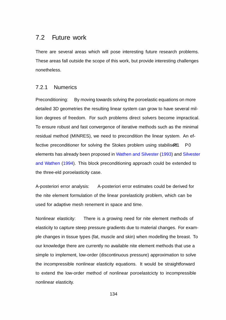
7.2 Future work

There are several areas which will pose interesting future research problems.

These areas fall outside the scope of this work, but provide interesting challenges

nonetheless.

7.2.1 Numerics

Preconditioning: By moving towards solving the poroelastic equations on more

detailed 3D geometries the resulting linear system can grow to have several mil-

lion degrees of freedom. For such problems direct solvers become impractical.

To ensure robust and fast convergence of iterative methods such as the minimal

residual method (MINRES), we need to precondition the linear system. An ef-

fective preconditioner for solving the Stokes problem using stabilised P1 − P0

elements has already been proposed in Wathen and Silvester (1993) and Silvester

and Wathen (1994). This block preconditioning approach could be extended to

the three-field poroelasticity case.

A-posteriori error analysis: A-posteriori error estimates could be derived for

the finite element formulation of the linear porelasticity problem, which can be

used for adaptive mesh refinement in space and time.

Nonlinear elasticity: There is a growing need for finite element methods of

elasticity to capture steep pressure gradients due to material changes. For exam-

ple changes in tissue types (fat, muscle and skin) when modelling the breast. To

our knowledge there are currently no available finite element methods that use a

simple to implement, low-order (discontinuous pressure) approximation to solve

the incompressible nonlinear elasticity equations. It would be straightforward

to extend the low-order method of nonlinear poroelastcicty to incompressible

nonlinear elasticity.

134

7.2.2 Lung model

Validation: For this model to be of practical use it is crucial that it is properly

validated, this can be achieved by making use of different imaging modalities and

phantom studies where model predictions can be tested. Computed tomography

and 4D (dynamic) Magnetic resonance imaging (MRI) can be used to track dis-

placements and calculate volume changes of lung structures. MRI of gases such

as Hyperpolarised Xenon (Kaushik et al., 2011) and Helium 3 can be used to

infer the flow and diffusion of gases, and with the use of elastography we are

able to image stiffness and strain of lung tissue. Recently there has also been

development in using Hyperpolarised Helium 3 MRI to estimate flow velocities

and thus calculate pressure gradients (Patz et al., 2007).

Surgical planning: For patients with severe emphysema invasive surgical pro-

cedures such as lung volume reduction surgery (LVRS) and endobronchial valve

placement are possible treatments. During LVRS part of the lung is excised in

order to improve the configuration of the thoracic cavity, improve elastic recoil,

and allow for improved lung inflation of the remaining and presumably better

preserved tissue (Criner et al., 2011). Due to the high post-surgery mortality

rate of around 5 − 10 percent for LVRS and the fact that only some patients

show an improvement with this therapy it is currently extremely challenging for

doctors to select patients that will benefit from this invasive surgery. Boundary

conditions allowing the lung surface to slide along the pleural cavity would have

to be implemented, to allow for the removal of whole lobes in the model. A suc-

cessful computational lung model would predict how much a particular patient

will benefit from this high risk treatment, and help clinicians decide whether or

not to perform surgery.

135

In addition to LVRS, various minimally invasive bronchoscopic approaches

that also try to cure hyperinflation are being investigated. These include valves

that reduce the air flow into the treated lobe during inspiration, stents that

keep communications between pulmonary parenchyma and the segmental air-

ways open, and lung volume reduction coils that aim to cause parenchymal com-

pression and reduce the size of the hyperinflated tissue. More investigation into

these techniques and which patients are best suited for a particular treatment is

needed. A further developed computational lung model could be used to inves-

tigate these approaches and help surgeons plan for surgery by trialling different

approaches in silico before the operation.

Modelling other organs: Finally, the proposed methodology for solving the

lung model could also be adapted to model other biological tissues where blood

vessels flow through and interact with a deforming tissue. For example, when

modelling perfusion of blood flow in the beating myocardium (Chapelle et al.,

2010; Cookson et al., 2012), modelling brain oedema (Li et al., 2010) or hydro-

cephalus (Wirth and Sobey, 2006), or microcirculation of blood and interstitial

fluid in the liver lobule (Leungchavaphongse, 2013).

136

7.3 Final remarks

It is clear that there is a great requirement for effective simulation capabilities

when it comes to modelling biological tissues. The possibility of robust and

efficient simulations will enable researchers in the fields of medical device design,

clinical treatment planning, and basic research. Although we have made some

progress towards achieving this, still much research needs to be done, especially

on how to implement models on high performance computers, to make detailed

parameter studies possible.

The long term modelling aim of this project is to develop software which

can accurately predict the ventilation and tissue deformation in the lungs. We

have shown that, although such software would still be many years away from

completion, requiring a great deal of work in the modelling, validation and bio-

mechanical experimentation aspects, the aim is feasible and already computa-

tionally tractable.

137

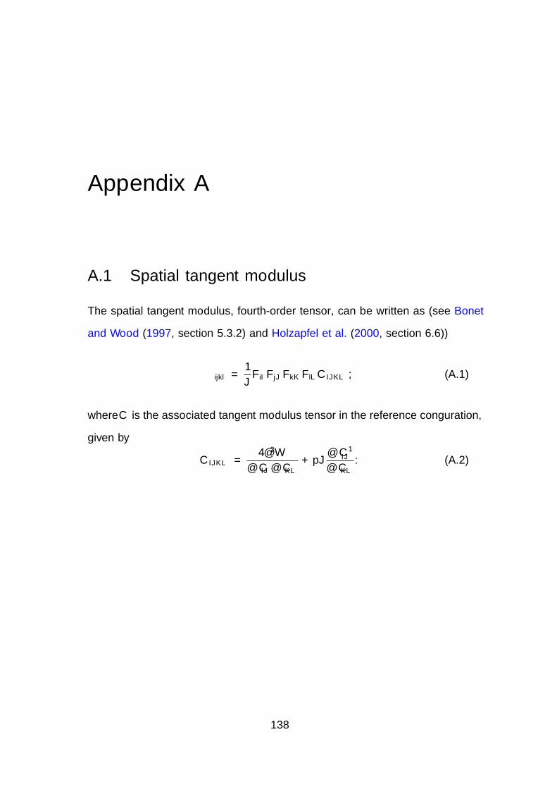
Appendix A

A.1 Spatial tangent modulus

The spatial tangent modulus, fourth-order tensor, can be written as (see Bonet

and Wood (1997, section 5.3.2) and Holzapfel et al. (2000, section 6.6))

Θijkl =1

JFiIFjJFkKFlLCIJKL, (A.1)

where C is the associated tangent modulus tensor in the reference configuration,

given by

CIJKL =4∂2W

∂CIJ∂CKL+ pJ

∂C−1IJ

∂CKL. (A.2)

138

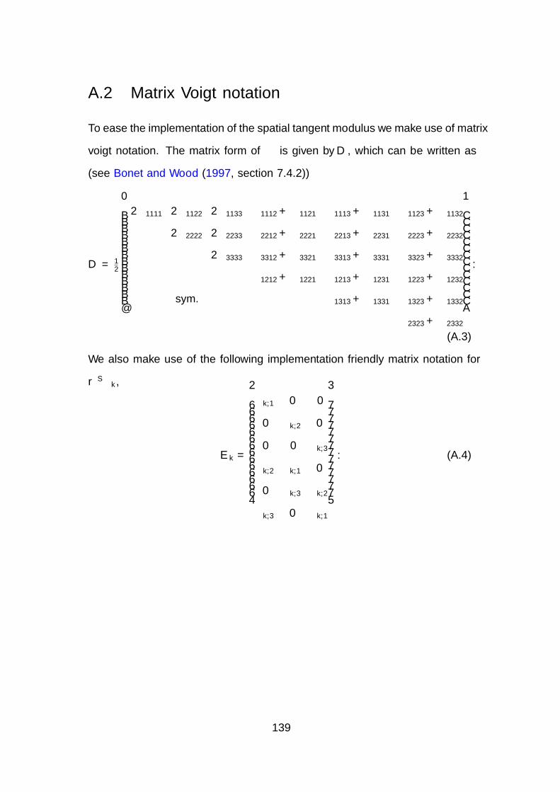
A.2 Matrix Voigt notation

To ease the implementation of the spatial tangent modulus we make use of matrix

voigt notation. The matrix form of Θ is given by D, which can be written as

(see Bonet and Wood (1997, section 7.4.2))

D = 12

2Θ1111 2Θ1122 2Θ1133 Θ1112 + Θ1121 Θ1113 + Θ1131 Θ1123 + Θ1132

2Θ2222 2Θ2233 Θ2212 + Θ2221 Θ2213 + Θ2231 Θ2223 + Θ2232

2Θ3333 Θ3312 + Θ3321 Θ3313 + Θ3331 Θ3323 + Θ3332

Θ1212 + Θ1221 Θ1213 + Θ1231 Θ1223 + Θ1232

sym. Θ1313 + Θ1331 Θ1323 + Θ1332

Θ2323 + Θ2332

.

(A.3)

We also make use of the following implementation friendly matrix notation for

∇Sφk,

Ek =

φk,1 0 0

0 φk,2 0

0 0 φk,3

φk,2 φk,1 0

0 φk,3 φk,2

φk,3 0 φk,1

. (A.4)

139

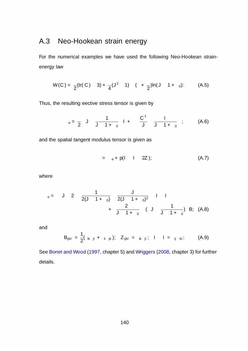
A.3 Neo-Hookean strain energy

For the numerical examples we have used the following Neo-Hookean strain-

energy law

W (C) =µ

2(tr(C)− 3) +

Λ

4(J2 − 1)− (µ+

Λ

2)ln(J − 1 + φ0). (A.5)

Thus, the resulting effective stress tensor is given by

σe =Λ

2

(J − 1

J − 1 + φ0

)I + µ

(CT

J− I

J − 1 + φ0

), (A.6)

and the spatial tangent modulus tensor is given as

Θ = Θe + p(I ⊗ I − 2Z), (A.7)

where

Θe =

[ΛJ − 2µ

(1

2(J − 1 + φ0)− J

2(J − 1 + φ0)2

)]I ⊗ I

+

[2µ

J − 1 + φ0

− Λ(J − 1

J − 1 + φ0

)

]B, (A.8)

and

Bijkl =1

2(δikδjl + δilδjk), Zijkl = δikδjl, I ⊗ I = δijδkl. (A.9)

See Bonet and Wood (1997, chapter 5) and Wriggers (2008, chapter 3) for further

details.

140

Bibliography

Albaiceta, G. M., Blanch, L., and Lucangelo, U. Static pressure–volume curves

of the respiratory system: were they just a passing fad? Current Opinion in

Critical Care, 14(1):80–86, 2008.

Almeida, E. and Spilker, R. Finite element formulations for hyperelastic trans-

versely isotropic biphasic soft tissues. Computer Methods in Applied Mechanics

and Engineering, 151(3):513–538, 1998.

Amestoy, P. R., Duff, I. S., and L’Excellent, J. Multifrontal parallel distributed

symmetric and unsymmetric solvers. Computer Methods in Applied Mechanics

and Engineering, 184(2):501–520, 2000.

Armstrong, C., Lai, W., and Mow, V. An analysis of the unconfined compression

of articular cartilage. Journal of Biomechanical Engineering, 106(2):165–173,

1984.

Arthurs, C. Effcient Simulation of Cardiac Electrical Propagation using Adaptive

High-Order Finite Elements. PhD thesis, University of Oxford, 2012.

Asner, L. Efficient numerical methods for the solution of coupled multiphysics

problems. PhD thesis, University of Oxford, 2013.

Ateshian, G. A., Maas, S., and Weiss, J. A. Finite element algorithm for friction-

less contact of porous permeable media under finite deformation and sliding.

Journal of Biomechanical Engineering, 132(6):061006, 2010.

141

Babuska, I. Error-bounds for finite element method. Numerische Mathematik,

16(4):322–333, 1971.

Badia, S., Quaini, A., and Quarteroni, A. Coupling Biot and Navier-Stokes

equations for modelling fluid-poroelastic media interaction. Journal of Com-

putational Physics, 228(21):7986–8014, 2009.

Barucq, H., Madaune-Tort, M., and Saint-Macary, P. Some existence-uniqueness

results for a class of one-dimensional nonlinear Biot models. Nonlinear Anal-

ysis: Theory, Methods & Applications, 61(4):591–612, 2005.

Bates, J. Lung mechanics: an inverse modeling approach. Cambridge University

Press, 2009.

Bernabeu, M. An open source HPC-enabled model of cardiac defibrillation of the

human heart. PhD thesis, University of Oxford, 2011.

Bochev, P. and Dohrmann, C. A computational study of stabilized, low-order C0

finite element approximations of Darcy equations. Computational Mechanics,

38(4):323–333, 2006.

Boer, R. Trends in continuum mechanics of porous media. Springer, 2005.

Bonet, J. and Wood, R. Nonlinear continuum mechanics for finite element anal-

ysis. Cambridge University Press, 1997.

Bordas, R., Lefevre, C., Veeckmans, B., Pitt-Francis, J., Fetita, C., Kay, D.,

Siddiqui, S., and Burrowes, K. Development and validation of patient-based

complete conducting airways models. PLoS ONE (submitted), 2014.

Bowen, R. Porous elasticity: Lectures on the elasticity of porous materi-

als as an application of the theory of mixtures. Available electronically

142

from http://repository.tamu.edu/handle/1969.1/91297, 2010. URL http://

repository.tamu.edu/handle/1969.1/91297.

Brenner, S. C. and Scott, L. R. The mathematical theory of finite element meth-

ods, volume 15. Springer, 2008.

Brezzi, F. and Fortin, M. Mixed and hybrid finite element methods. Springer-

Verlag, 1991a.

Brezzi, F. and Fortin, M. Mixed and hybrid finite element methods. Springer-

Verlag New York, Inc., 1991b.

Burman, E. and Hansbo, P. A unified stabilized method for Stokes’ and Darcy’s

equations. Journal of Computational and Applied Mathematics, 198(1):35–51,

2007.

Chapelle, D., Gerbeau, J., Sainte-Marie, J., and Vignon-Clementel, I. A poroe-

lastic model valid in large strains with applications to perfusion in cardiac

modeling. Computational Mechanics, 46(1):91–101, 2010.

Chapelle, D. and Moireau, P. General coupling of porous flows and hyperelastic

formulations—from thermodynamics principles to energy balance and com-

patible time schemes. European Journal of Mechanics-B/Fluids, 46(0):82–96,

2014.

Ciarlet, P. G. The finite element method for elliptic problems. Elsevier, 1978.

Cookson, A., Lee, J., Michler, C., Chabiniok, R., Hyde, E., Nordsletten, D.,

Sinclair, M., Siebes, M., and Smith, N. A novel porous mechanical framework

for modelling the interaction between coronary perfusion and myocardial me-

chanics. Journal of Biomechanics, 45(5):850 – 855, 2012.

143

Cotes, J. E., Chinn, D. J., and Miller, M. R. Lung function: physiology, mea-

surement and application in medicine. John Wiley & Sons, 2009.

Coussy, O. Poromechanics. John Wiley & Sons Inc, 2004.

Coussy, O., Dormieux, L., and Detournay, E. From mixture theory to Biot’s

approach for porous media. International Journal of Solids and Structures, 35

(34):4619–4635, 1998.

Criner, G. J., Cordova, F., Sternberg, A. L., and Martinez, F. J. The National

Emphysema Treatment Trial (NETT) part II: lessons learned about lung vol-

ume reduction surgery. American Journal of Respiratory and Critical Care

Medicine, 184(8):881–893, 2011.

De Wilde, R., Clement, J., Hellemans, J., Decramer, M., Demedts, M., Boving,

R., and Van de Woestijne, K. Model of elasticity of the human lung. Journal

of Applied Physiology, 51(2):254–261, 1981.

Di Pietro, D. A. and Ern, A. Mathematical aspects of discontinuous Galerkin

methods. Springer, 2011.

Elman, H., Silvester, D., and Wathen, A. Finite elements and fast iterative

solvers: with applications in incompressible fluid dynamics. Oxford University

Press, USA, 2005.

Fang, Q. and Boas, D. A. Tetrahedral mesh generation from volumetric binary

and grayscale images. In Biomedical Imaging: From Nano to Macro, 2009.

ISBI’09. IEEE International Symposium, pages 1142–1145. IEEE, 2009.

Feng, X. and He, Y. Fully discrete finite element approximations of a polymer

gel model. SIAM Journal on Numerical Analysis, 48(6):2186–2217, 2010.

144

Ferronato, M., Castelletto, N., and Gambolati, G. A fully coupled 3-D mixed

finite element model of Biot consolidation. Journal of Computational Physics,

229(12):4813–4830, 2010.

Freed, A. D. and Einstein, D. R. An implicit elastic theory for lung parenchyma.

International Journal of Engineering Science, 62(0):31–47, 2013.

Fung, Y. Stress, deformation, and atelectasis of the lung. Circulation Research,

37(4):481–496, 1975.

Galban, C. J., Han, M. K., Boes, J. L., Chughtai, K. A., Meyer, C. R., Johnson,

T. D., Galban, S., Rehemtulla, A., Kazerooni, E. A., Martinez, F. J., et al.

Computed tomography-based biomarker provides unique signature for diag-

nosis of COPD phenotypes and disease progression. Nature Medicine, 18(11):

1711–1715, 2012.

Galbusera, F., Schmidt, H., Noailly, J., Malandrino, A., Lacroix, D., Wilke,

H., and Shirazi-Adl, A. Comparison of four methods to simulate swelling

in poroelastic finite element models of intervertebral discs. Journal of the

Mechanical Behavior of Biomedical Materials, 4(7):1234 – 1241, 2011.

Galie, P., Spilker, R., and Stegemann, J. A linear, biphasic model incorporating

a Brinkman term to describe the mechanics of cell-seeded collagen hydrogels.

Annals of Biomedical Engineering, 39(11):2767–2779, 2011.

Gonzalez, O. and Stuart, A. A first course in continuum mechanics. Cambridge

University Press, 2008.

Haga, J., Osnes, H., and Langtangen, H. On the causes of pressure oscillations in

low-permeable and low-compressible porous media. International Journal for

Numerical and Analytical Methods in Geomechanics, 36(12):1507–1522, 2012.

145

Harris, R. S. Pressure-volume curves of the respiratory system. Respiratory Care,

50(1):78–99, 2005.

Hedges, K. A Computational Model of Forced Expiration Through Anatomical

Airways in Health and Disease. PhD thesis, The University of Auckland, 2009.

Heinrich, H., Jenkinson, M., Brady, M., and Schnabel, J. A. MRF-based de-

formable registration and ventilation estimation of lung ct. Medical Imaging,

IEEE Transactions on, 32(7):1239–1248, 2013.

Holmes, M. and Mow, V. The nonlinear characteristics of soft gels and hydrated

connective tissues in ultrafiltration. Journal of Biomechanics, 23(11):1145–

1156, 1990.

Holzapfel, G., Schulze-Bauer, C., and Stadler, M. Mechanics of angioplasty:

Wall, balloon and stent. ASME Applied Mechanics, 242(46):141–156, 2000.

Hyde, E. Multi-Scale Parameterisation of Static and Dynamic Continuum

Porous Perfusion Models using Discrete Anatomical Data. PhD thesis, Uni-

versity of Oxford, 2013.

Ismail, M., Comerford, A., and Wall, W. Coupled and reduced dimensional mod-

eling of respiratory mechanics during spontaneous breathing. International

Journal for Numerical Methods in Biomedical Engineering, 29(11):1285–1305,

2013.

Jahani, N., Yin, Y., Hoffman, E. A., and Lin, C.-L. Assessment of regional non-

linear tissue deformation and air volume change of human lungs via image

registration. Journal of Biomechanics, 47(7):1626–1633, 2014.

Kaushik, S., Cleveland, Z., Cofer, G., Metz, G., Beaver, D., Nouls, J., Kraft,

M., Auffermann, W., Wolber, J., McAdams, H., et al. Diffusion-weighted

146

hyperpolarized 129Xe MRI in healthy volunteers and subjects with chronic

obstructive pulmonary disease. Magnetic Resonance in Medicine, 65(4):1154–

1165, 2011.

Khaled, A.-R. and Vafai, K. The role of porous media in modeling flow and heat

transfer in biological tissues. International Journal of Heat and Mass Transfer,

46(26):4989–5003, 2003.

Kim, J., Tchelepi, H., and Juanes, R. Stability and convergence of sequen-

tial methods for coupled flow and geomechanics: Fixed-stress and fixed-strain

splits. Computer Methods in Applied Mechanics and Engineering, 200(13):

1591–1606, 2011.

Kirk, B. S., Peterson, J. W., Stogner, R. H., and Carey, G. F. libMesh: A

C++ Library for Parallel Adaptive Mesh Refinement/Coarsening Simulations.

Engineering with Computers, 22(3–4):237–254, 2006.

Kowalczyk, P. and Kleiber, M. Modelling and numerical analysis of stresses and

strains in the human lung including tissue-gas interaction. European Journal

of Mechanics. A. Solids, 13(3):367–393, 1994.

Lai, W. and Mow, V. Drag-induced compression of articular cartilage during a

permeation experiment. Biorheology, 17(1-2):111, 1980.

Lande, B. and Mitzner, W. Analysis of lung parenchyma as a parametric porous

medium. Journal of Applied Physiology, 101(3):926–933, 2006.

Lawrence Berkeley National Laboratory. LBNL LungLab Tour. http://www.

whywasteyourbreath.com/images.html, 1995.

Leary, D., Winkler, T., Braune, A., and Maksym, G. N. Effects of airway tree

asymmetry on the emergence and spatial persistence of ventilation defects.

Journal of Applied Physiology, 117(4):353–362, 2014.

147

Lee, G., Tseng, N., and Yuan, Y. Finite element modeling of lungs including

interlobar fissures and the heart cavity. Journal of Biomechanics, 16(9):679–

690, 1983.

Leungchavaphongse, K. Mathematical modelling of the liver microcirculation.

PhD thesis, Imperial College London, 2013.

Levenston, M., Frank, E., and Grodzinsky, A. Variationally derived 3-field finite

element formulations for quasistatic poroelastic analysis of hydrated biological

tissues. Computer Methods in Applied Mechanics and Engineering, 156(1-4):

231–246, 1998.

Lewis, M. A. and Owen, M. R. The mechanics of lung tissue under high-frequency

ventilation. SIAM Journal on Applied Mathematics, 61(5):1731–1761, 2001.

Li, C., Borja, R., and Regueiro, R. Dynamics of porous media at finite strain.

Computer Methods in Applied Mechanics and Engineering, 193(36):3837–3870,

2004.

Li, H. and Li, Y. A discontinuous Galerkin finite element method for swelling

model of polymer gels. Journal of Mathematical Analysis and Applications,

398(1):11–25, 2012.

Li, X., Holst, H., Ho, J., and Kleiven, S. Three dimensional poroelastic simulation

of brain edema: Initial studies on intracranial pressure. In World Congress

on Medical Physics and Biomedical Engineering, pages 1478–1481. Springer,

2010.

Lipnikov, K. Numerical methods for the Biot model in poroelasticity. PhD thesis,

University of Houston, 2002.

Liu, R. Discontinuous Galerkin finite element solution for poromechanics. PhD

thesis, The University of Texas at Austin, 2004.

148

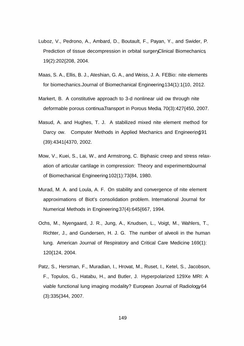
Luboz, V., Pedrono, A., Ambard, D., Boutault, F., Payan, Y., and Swider, P.

Prediction of tissue decompression in orbital surgery. Clinical Biomechanics,

19(2):202–208, 2004.

Maas, S. A., Ellis, B. J., Ateshian, G. A., and Weiss, J. A. FEBio: finite elements

for biomechanics. Journal of Biomechanical Engineering, 134(1):1–10, 2012.

Markert, B. A constitutive approach to 3-d nonlinear fluid flow through finite

deformable porous continua. Transport in Porous Media, 70(3):427–450, 2007.

Masud, A. and Hughes, T. J. A stabilized mixed finite element method for

Darcy flow. Computer Methods in Applied Mechanics and Engineering, 191

(39):4341–4370, 2002.

Mow, V., Kuei, S., Lai, W., and Armstrong, C. Biphasic creep and stress relax-

ation of articular cartilage in compression: Theory and experiments. Journal

of Biomechanical Engineering, 102(1):73–84, 1980.

Murad, M. A. and Loula, A. F. On stability and convergence of finite element

approximations of Biot’s consolidation problem. International Journal for

Numerical Methods in Engineering, 37(4):645–667, 1994.

Ochs, M., Nyengaard, J. R., Jung, A., Knudsen, L., Voigt, M., Wahlers, T.,

Richter, J., and Gundersen, H. J. G. The number of alveoli in the human

lung. American Journal of Respiratory and Critical Care Medicine, 169(1):

120–124, 2004.

Patz, S., Hersman, F., Muradian, I., Hrovat, M., Ruset, I., Ketel, S., Jacobson,

F., Topulos, G., Hatabu, H., and Butler, J. Hyperpolarized 129Xe MRI: A

viable functional lung imaging modality? European Journal of Radiology, 64

(3):335–344, 2007.

149

Pedley, T., Schroter, R., and Sudlow, M. Energy losses and pressure drop in

models of human airways. Respiration Physiology, 9(3):371–386, 1970a.

Pedley, T., Schroter, R., and Sudlow, M. The prediction of pressure drop and

variation of resistance within the human bronchial airways. Respiration Phys-

iology, 9(3):387–405, 1970b.

Phillips, P. J. and Wheeler, M. F. A coupling of mixed and continuous Galerkin

finite element methods for poroelasticity I: the continuous in time case. Com-

putational Geosciences, 11(2):131–144, 2007a.

Phillips, P. J. and Wheeler, M. F. A coupling of mixed and continuous Galerkin

finite element methods for poroelasticity II: the discrete-in-time case. Compu-

tational Geosciences, 11(2):145–158, 2007b.

Phillips, P. J. and Wheeler, M. F. A coupling of mixed and discontinu-

ous Galerkin finite-element methods for poroelasticity. Computational Geo-

sciences, 12(4):417–435, 2008.

Phillips, P. J. and Wheeler, M. F. Overcoming the problem of locking in lin-

ear elasticity and poroelasticity: an heuristic approach. Computational Geo-

sciences, 13(1):5–12, 2009.

Rajagopal, V., Nielsen, P. M., and Nash, M. P. Modeling breast biomechanics for

multi-modal image analysis—successes and challenges. Wiley Interdisciplinary

Reviews: Systems Biology and Medicine, 2(3):293–304, 2010.

Ranieri, V. M., Giuliani, R., Fiore, T., Dambrosio, M., and Milic-Emili, J.

Volume-pressure curve of the respiratory system predicts effects of PEEP in

ARDS: ‘occlusion’ versus ‘constant flow’ technique. American Journal of Res-

piratory and Critical Care Medicine, 149(1):19–27, 1994.

150

Raviart, P.-A. and Thomas, J.-M. A mixed finite element method for 2-nd order

elliptic problems. In Mathematical Aspects of Finite Element Methods, volume

606, pages 292–315. Springer, 1977.

Rittner, F. and Doring, M. Curves and loops in mechanical ventilation. Drager

Medical Incorporated, 2005.

Sauter, M. and Wieners, C. Robust estimates for the approximation of the

dynamic consolidation problem. IMA Journal of Numerical Analysis, 30(3):

832–856, 2010.

Showalter, R. Diffusion in poro-elastic media. Journal of Mathematical Analysis

and Applications, 251(1):310–340, 2000.

Silvester, D. and Wathen, A. Fast iterative solution of stabilised Stokes systems

part II: Using general block preconditioners. SIAM Journal on Numerical

Analysis, 31(5):1352–1367, 1994.

Suki, B. and Bates, J. Lung tissue mechanics as an emergent phenomenon.

Journal of Applied Physiology, 110(4):1111–1118, 2011.

Swan, A., Clark, A., and Tawhai, M. A computational model of the topographic

distribution of ventilation in healthy human lungs. Journal of Theoretical

Biology, 300:222 – 231, 2012.

Tawhai, M. H., Nash, M. P., Lin, C.-L., and Hoffman, E. A. Supine and prone

differences in regional lung density and pleural pressure gradients in the human

lung with constant shape. Journal of Applied Physiology, 107(3):912–920, 2009.

Tawhai, M. and Lin, C. Image-based modeling of lung structure and function.

Journal of Magnetic Resonance Imaging, 32(6):1421–1431, 2010.

151

Tawhai, M., Nash, M., and Hoffman, E. An Imaging-based Computational Ap-

proach to Model Ventilation Distribution and Soft-tissue Deformation in the

Ovine Lung. Academic Radiology, 13(1):113–120, 2006.

Thomee, V. Galerkin finite element methods for parabolic problems. Springer,

2006.

Un, K. and Spilker, R. L. A penetration-based finite element method for hy-

perelastic 3D biphasic tissues in contact. Part II: finite element simulations.

Journal of Biomechanical Engineering, 128(6):934–942, 2006.

Venegas, J. G., Winkler, T., Musch, G., Melo, M. F. V., Layfield, D., Tgavalekos,

N., Fischman, A. J., Callahan, R. J., Bellani, G., and Harris, R. S. Self-

organized patchiness in asthma as a prelude to catastrophic shifts. Nature,

434(7034):777–782, 2005.

Verfurth, R. A posteriori error estimators for convection-diffusion equations.

Numerische Mathematik, 80(4):641–663, 1998.

Vuong, A.-T., Yoshihara, L., and Wall, W. A general approach for modeling

interacting flow through porous media under finite deformations. Computer

Methods in Applied Mechanics and Engineering, 283(0):1240–1259, 2015.

Wathen, A. and Silvester, D. Fast iterative solution of stabilised Stokes systems.

Part I: Using simple diagonal preconditioners. SIAM Journal on Numerical

Analysis, 30(3):630–649, 1993.

Weichert, L. Computational Modeling of Multi-Field and Multi-Scale Phenomena

in Respiratory Mechanics . PhD thesis, Technischen Universitat Munchen,

2011.

Werner, R., Ehrhardt, J., Schmidt, R., and Handels, H. Patient-specific finite

152

element modeling of respiratory lung motion using 4D CT image data. Medical

physics, 36(5):1500–1511, 2009.

West, J. Respiratory physiology: the essentials. Lippincott Williams & Wilkins,

2008.

Wheeler, M. F. and Gai, X. Iteratively coupled mixed and Galerkin finite ele-

ment methods for poro-elasticity. Numerical Methods for Partial Differential

Equations, 23(4):785–797, 2007.

White, J. and Borja, R. Stabilized low-order finite elements for coupled solid-

deformation/fluid-diffusion and their application to fault zone transients. Com-

puter Methods in Applied Mechanics and Engineering, 197(49):4353–4366,

2008.

White, J. A. and Borja, R. I. Block-preconditioned Newton–Krylov solvers for

fully coupled flow and geomechanics. Computational Geosciences, 15(4):647–

659, 2011.

Wirth, B. and Sobey, I. An axisymmetric and fully 3D poroelastic model for

the evolution of hydrocephalus. Mathematical Medicine and Biology, 23(4):

363–388, 2006.

Wriggers, P. Nonlinear finite element methods. Springer Verlag, 2008.

Yi, S.-Y. A coupling of nonconforming and mixed finite element methods for

Biot’s consolidation model. Numerical Methods for Partial Differential Equa-

tions, 2013.

Yin, Y., Choi, J., Hoffman, E. A., Tawhai, M. H., and Lin, C.-L. Simulation

of pulmonary air flow with a subject-specific boundary condition. Journal of

Biomechanics, 43(11):2159–2163, 2010.

153

Yin, Y., Choi, J., Hoffman, E. A., Tawhai, M. H., and Lin, C.-L. A multiscale

MDCT image-based breathing lung model with time-varying regional ventila-

tion. Journal of Computational Physics, 244(0):168–192, 2013.

Zenısek, A. The existence and uniqueness theorem in Biot’s consolidation theory.

Aplikace Matematiky, 29(3):194–211, 1984.

Zhang, T., Orton, N. P., Mackie, T. R., and Paliwal, B. R. Technical note:

A novel boundary condition using contact elements for finite element based

deformable image registration. Medical Physics, 31(9):2412–2415, 2004.

154