A long-term numerical solution for the insolation ...
25
A&A 428, 261–285 (2004) DOI: 10.1051/0004-6361:20041335 c ESO 2004 Astronomy & Astrophysics A long-term numerical solution for the insolation quantities of the Earth J. Laskar 1 , P. Robutel 1 , F. Joutel 1 , M. Gastineau 1 , A. C. M. Correia 1,2 , and B. Levrard 1 1 Astronomie et Systèmes Dynamiques, IMCCE – CNRS UMR8028, 77 Av. Denfert-Rochereau, 75014 Paris, France e-mail: [email protected] 2 Departamento de Física da Universidade de Aveiro, Campus Universitário de Santiago, 3810-193 Aveiro, Portugal Received 23 May 2004 / Accepted 11 August 2004 Abstract. We present here a new solution for the astronomical computation of the insolation quantities on Earth spanning from −250 Myr to 250 Myr. This solution has been improved with respect to La93 (Laskar et al. 1993) by using a direct integration of the gravitational equations for the orbital motion, and by improving the dissipative contributions, in particular in the evolution of the Earth–Moon System. The orbital solution has been used for the calibration of the Neogene period (Lourens et al. 2004), and is expected to be used for age calibrations of paleoclimatic data over 40 to 50 Myr, eventually over the full Palaeogene period (65 Myr) with caution. Beyond this time span, the chaotic evolution of the orbits prevents a precise determination of the Earth’s motion. However, the most regular components of the orbital solution could still be used over a much longer time span, which is why we provide here the solution over 250 Myr. Over this time interval, the most striking feature of the obliquity solution, apart from a secular global increase due to tidal dissipation, is a strong decrease of about 0.38 degree in the next few millions of years, due to the crossing of the s 6 + g 5 − g 6 resonance (Laskar et al. 1993). For the calibration of the Mesozoic time scale (about 65 to 250 Myr), we propose to use the term of largest amplitude in the eccentricity, related to g 2 − g 5 , with a fixed frequency of 3.200 /yr, corresponding to a period of 405 000 yr. The uncertainty of this time scale over 100 Myr should be about 0.1%, and 0.2% over the full Mesozoic era. Key words. chaos – celestial mechanics – ephemerides – Earth 1. Introduction Due to gravitational planetary perturbations, the elliptical ele- ments of the orbit of the Earth are slowly changing in time, as is the orientation of the planet’s spin axis. These changes induce variations of the insolation received on the Earth’s surface. The first computation of the secular variations of the Earth’s or- bital elements were made by Lagrange (1781, 1782), and then Pontécoulant (1834), but it was the work of Agassiz (1840), showing geological evidence of past ice ages, that triggered the search for a correlation between the geological evidence of large climatic changes, and the variations of the Earth’s astro- nomical parameters. Shortly after, Adhémar (1842) proposed that these climatic variations originated from the precession of the Earth’s rotation axis. After the publication of a more precise solution of the Earth by Le Verrier (1856), that took into account the secular pertur- bations of all main planets except for Neptune, Croll (1890) proposed that the variation of the Earth’s eccentricity was also an important parameter for the understanding of the past cli- mates of the Earth. The first computations of the variations of the obliquity (angle between the equator and orbital plane) due to the sec- ular variations of the orbital plane of the Earth are due to Pilgrim (1904), and were later used by Milankovitch (1941) to establish his theory of the Earth’s insolation parameters. Since then, the understanding of the climate response to the orbital forcing has evolved, but all the necessary ingredients for the insolation computations were present in Milankovitch’s work. The revival of the Milankovitch theory of paleoclimate can be related to the landmark work of Hays et al. (1976), that established a correlation between astronomical forcing and the δ 18 O records over the past 500 kyr. The Milankovitch the- ory has since been confirmed overall with variations in the cli- mate response to the insolation forcing (see Imbrie & Imbrie 1979; Imbrie 1982, for more historical details; and Zachos et al. 2001; Grastein et al. 2004, for a recent review on the astronom- ical calibration of geological data). Since the work of Pilgrim (1904) and Milankovitch (1941), the orbital and precession quantities of the Earth have un- dergone several improvements. Le Verrier’s solution (1856) consisted in the linearized equations for the secular evolu- tion of the planetary orbits. Stockwell (1873), and Harzer (1895) added the planet Neptune to Le Verrier’s computa- tions. A significant improvement is due to Hill (1897) who discovered that the proximity of a resonance in Jupiter and Saturn’s motion induces some important complements at the second order with respect to the masses. The solution of Article published by EDP Sciences and available at http://www.aanda.org or http://dx.doi.org/10.1051/0004-6361:20041335
Transcript of A long-term numerical solution for the insolation ...
A&A 428, 261–285 (2004)DOI: 10.1051/0004-6361:20041335c© ESO 2004
Astronomy&
Astrophysics
A long-term numerical solution for the insolationquantities of the Earth
J. Laskar1, P. Robutel1, F. Joutel1, M. Gastineau1, A. C. M. Correia1,2, and B. Levrard1
1 Astronomie et Systèmes Dynamiques, IMCCE – CNRS UMR8028, 77 Av. Denfert-Rochereau, 75014 Paris, Francee-mail: [email protected]
2 Departamento de Física da Universidade de Aveiro, Campus Universitário de Santiago, 3810-193 Aveiro, Portugal
Received 23 May 2004 / Accepted 11 August 2004
Abstract. We present here a new solution for the astronomical computation of the insolation quantities on Earth spanningfrom −250 Myr to 250 Myr. This solution has been improved with respect to La93 (Laskar et al. 1993) by using a directintegration of the gravitational equations for the orbital motion, and by improving the dissipative contributions, in particularin the evolution of the Earth–Moon System. The orbital solution has been used for the calibration of the Neogene period(Lourens et al. 2004), and is expected to be used for age calibrations of paleoclimatic data over 40 to 50 Myr, eventuallyover the full Palaeogene period (65 Myr) with caution. Beyond this time span, the chaotic evolution of the orbits prevents aprecise determination of the Earth’s motion. However, the most regular components of the orbital solution could still be usedover a much longer time span, which is why we provide here the solution over 250 Myr. Over this time interval, the moststriking feature of the obliquity solution, apart from a secular global increase due to tidal dissipation, is a strong decrease ofabout 0.38 degree in the next few millions of years, due to the crossing of the s6 + g5 − g6 resonance (Laskar et al. 1993).For the calibration of the Mesozoic time scale (about 65 to 250 Myr), we propose to use the term of largest amplitude in theeccentricity, related to g2 − g5, with a fixed frequency of 3.200′′/yr, corresponding to a period of 405 000 yr. The uncertainty ofthis time scale over 100 Myr should be about 0.1%, and 0.2% over the full Mesozoic era.
Key words. chaos – celestial mechanics – ephemerides – Earth
1. Introduction
Due to gravitational planetary perturbations, the elliptical ele-ments of the orbit of the Earth are slowly changing in time, as isthe orientation of the planet’s spin axis. These changes inducevariations of the insolation received on the Earth’s surface. Thefirst computation of the secular variations of the Earth’s or-bital elements were made by Lagrange (1781, 1782), and thenPontécoulant (1834), but it was the work of Agassiz (1840),showing geological evidence of past ice ages, that triggeredthe search for a correlation between the geological evidence oflarge climatic changes, and the variations of the Earth’s astro-nomical parameters. Shortly after, Adhémar (1842) proposedthat these climatic variations originated from the precession ofthe Earth’s rotation axis.
After the publication of a more precise solution of the Earthby Le Verrier (1856), that took into account the secular pertur-bations of all main planets except for Neptune, Croll (1890)proposed that the variation of the Earth’s eccentricity was alsoan important parameter for the understanding of the past cli-mates of the Earth.
The first computations of the variations of the obliquity(angle between the equator and orbital plane) due to the sec-ular variations of the orbital plane of the Earth are due to
Pilgrim (1904), and were later used by Milankovitch (1941) toestablish his theory of the Earth’s insolation parameters. Sincethen, the understanding of the climate response to the orbitalforcing has evolved, but all the necessary ingredients for theinsolation computations were present in Milankovitch’s work.
The revival of the Milankovitch theory of paleoclimatecan be related to the landmark work of Hays et al. (1976),that established a correlation between astronomical forcing andthe δ18O records over the past 500 kyr. The Milankovitch the-ory has since been confirmed overall with variations in the cli-mate response to the insolation forcing (see Imbrie & Imbrie1979; Imbrie 1982, for more historical details; and Zachos et al.2001; Grastein et al. 2004, for a recent review on the astronom-ical calibration of geological data).
Since the work of Pilgrim (1904) and Milankovitch (1941),the orbital and precession quantities of the Earth have un-dergone several improvements. Le Verrier’s solution (1856)consisted in the linearized equations for the secular evolu-tion of the planetary orbits. Stockwell (1873), and Harzer(1895) added the planet Neptune to Le Verrier’s computa-tions. A significant improvement is due to Hill (1897) whodiscovered that the proximity of a resonance in Jupiter andSaturn’s motion induces some important complements at thesecond order with respect to the masses. The solution of
Article published by EDP Sciences and available at http://www.aanda.org or http://dx.doi.org/10.1051/0004-6361:20041335

262 J. Laskar et al.: Insolation quantities of the Earth
Brouwer & Van Woerkom (1950) is essentially the solution ofLe Verrier and Stockwell, complemented by the higher ordercontributions computed by Hill. This solution was used for in-solation computations by Sharav & Boudnikova (1967a,b) withupdated values of the parameters, and later on by Vernekar(1972). The computations of Vernekar were actually used byHays et al. (1976).
The next improvement in the computation of the orbitaldata is by Bretagnon (1974), who computed the terms of secondorder and degree 3 in eccentricity and inclination in the secu-lar equations, but omitted the terms of degree 5 in the Jupiter-Saturn system from Hill (1897). This solution was then used byBerger (1978) for the computation of the precession and inso-lation quantities of the Earth, following Sharav & Boudnikova(1967a,b). All these works assumed implicitly that the motionof the Solar system was regular and that the solutions could beobtained as quasiperiodic series, using perturbation theory.
When Laskar (1984, 1985, 1986) computed in an extensiveway the secular equations for the Solar system, including allterms up to order 2 in the masses and 5 in eccentricity and in-clination, he realized that the traditional perturbative methodscould not be used for the integration of the secular equations,due to strong divergences that became apparent in the systemof the inner planets (Laskar 1984). This difficulty was over-come by switching to a numerical integration of the secularequations, which could be done in a very effective way, with avery large stepsize of 500 years. These computations provideda much more accurate solution for the orbital motion of theSolar system (Laskar 1986, 1988), which also included a fullsolution for the precession and obliquity of the Earth for inso-lation computations over 10 Myr (million of years). Extendinghis integration to 200 Myr, Laskar (1989, 1990) demonstratedthat the orbital motion of the planets, and especially of the ter-restrial planets, is chaotic, with an exponential divergence cor-responding to an increase of the error by a factor of 10 every10 Myr, thus destroying the hope to obtain a precise astronom-ical solution for paleoclimate studies over more than a few tensof million of years (Laskar 1999).
The first long term direct numerical integration (without av-eraging) of a realistic model of the Solar system, together withthe precession and obliquity equations, was made by Quinnet al. (1991) over 3 Myr. Over its range, this solution pre-sented very small differences with the updated secular solutionof Laskar et al. (1993) that was computed over 20 Myr, andhas since been extensively used for paleoclimate computationsunder the acronym La93. The orbital motion of the full Solarsystem has also been computed over 100 Myr by Sussman& Wisdom (1992), using a symplectic integrator with mixedvariables (Wisdom & Holman 1991), confirming the chaoticbehaviour found by Laskar (1989, 1990). Following the im-provement of computer technology, long term integrations ofrealistic models of the Solar system become more easy to per-form, but are still challenging when the time interval is the ageof the Solar system or if the accuracy of the model is compa-rable to the precision of short term planetary ephemeris. Thelongest integration was made over several billions of years byIto & Tanikawa (2002) with a Newtonian model that did notcontain general relativity or lunar contributions, while a recent
long term integration of the orbital motion of the Solar systemincluding general relativity, and where the Moon is resolvedwas made by Varadi et al. (2003) over about 50 Myr.
Here we present the result of the efforts that we have con-ducted in the past years in our group in order to obtain a newsolution for Earth paleoclimate studies over the Neogene pe-riod (≈23 Myr) and beyond. After a detailed analysis of themain limiting factors for long term integrations (Laskar 1999),and the design of new symplectic integrators (Laskar & Robutel2001), we have obtained a new numerical solution for both or-bital and rotational motion of the Earth that can be used overabout 50 Myr for paleoclimate studies, and even over longer pe-riods of time if only the most stable features of the solution areused. Apart from the use of a very complete dynamical modelfor the orbital motion of the planets, and of the new symplec-tic integrator of Laskar & Robutel (2001) (see next section), amajor change with respect to La93 (Laskar et al. 1993) is theconsideration, in the precession solution, of a more completemodel for the Earth–Moon tidal interactions (Sect. 4.1).
The present solution (La2004) or some of its previousvariants have already been distributed (Laskar 2001) andused for calibration of sedimentary records over extendedtime interval (Pälike 2002), and in particular for the con-struction of a new astronomically calibrated geological timescale for the Neogene period (Lourens et al. 2004). Thefull solution is available on the Web site www.imcce.fr/Equipes/ASD/insola/earth/earth.html, together with aset of routines for the computation of the insolation quantitiesfollowing (Laskar et al. 1993).
In addition to the numerical output of the orbital and rota-tional parameter of the Earth that is available on the Web site,we have made a special effort to provide in Sect. 8 very com-pact analytical approximations for the orbital and rotationalquantities of the Earth, that can be used in many cases fora better analytical understanding of the insolation variations.Finally, in the last sections, the stability of the solution La2004is discussed, as well as the possible chaotic transitions of thearguments present in the main secular resonances.
2. Numerical model
The orbital solutions La90−93 (Laskar 1990; Laskar et al.1993) were obtained by a numerical integration of the aver-aged equations of the Solar system, including the main generalrelativity and Lunar perturbations. The averaging process wasperformed using dedicated computer algebra routines. The re-sulting equations were huge, with about 150 000 polynomialterms, but as the short period terms were no longer present,these equations could be integrated with a step size of 200to 500 years, allowing very extensive long term orbital com-putations for the Solar system.
Although these averaged equations solutions could be im-proved by some new adjustment of the initial conditions andparameters (Laskar et al. 2004), it appears that because of theimprovements of computer technology, it becomes now pos-sible to obtain more precise results over a few tens of mil-lion of years using a more direct numerical integration ofthe gravitational equations, and this is how the present new

J. Laskar et al.: Insolation quantities of the Earth 263
Table 1. Main constants used in La2004. IAU76 refers to the resolutions of the International Astronmical Union of 1976, IERS1992,and IERS2000, refers to the IERS conventions (McCarthy 1992; McCarthy & Petit 2004).
Symbol Value Name Ref.
ε0 84 381.448 Obliquity of the ecliptic at J2000.0 IAU76
ω0 7.292115 × 10⁻⁵ rad s−1 Mean angular velocity of the Earth at J2000.0 IERS2000
ψ0 5029.0966 ′′/cy Precession constant IERS2000
δψ0 −0.29965 ′′/cy Correction to the precession IERS2000
k2 0.305 k2 of the Earth (Lambeck 1988)
k2M 0.0302 k2 of the Moon (Yoder 1995)
∆t 639 s Time lag of the Earth
∆tM 7055 s Time lag of the Moon
J2E 0.0010826362 Dynamical form-factor for the Earth IERS1992
J2M 0.000202151 Dynamical form-factor for the Moon IERS1992
J2S 2. × 10−7 Dynamical form-factor for the Sun IERS2000
RE 6378.1366 km Equatorial radius of the Earth IERS2000
RM 1738 km Equatorial radius of the Moon IAU76
Rsun 696 000 000 m Equatorial radius of the Sun IAU76
GS 1.32712442076 × 10²⁰ m3 s−2 Heliocentric gravitational constant IERS2000
Mmer 6 023 600 Sun – Mercury mass ratio IERS1992
Mven 408 523.71 Sun – Venus mass ratio IERS1992
Mear 328 900.56 Sun – Earth and Moon mass ratio IERS1992
Mmar 3 098 708 Sun – Mars mass ratio IERS1992
Mjup 1047.3486 Sun – Jupiter and satellites mass ratio IERS1992
Msat 3497.9 Sun – Saturn and satellites mass ratio IERS1992
Mura 22 902.94 Sun – Uranus and satellites mass ratio IERS1992
Mnep 19 412.24 Sun – Neptune and satellites mass ratio IERS1992
Mplu 135 000 000 Sun – Pluto and Charon mass ratio IERS1992
µ 0.0123000383 Moon-Earth mass ratio IERS2000
solution La2004 is obtained. A detailed account of the dynami-cal equations and numerical integrator is not in the scope of thepresent paper, but will be made in a forthcoming publication.Nevertheless, we will report here on the main issues concern-ing the numerical integrator, and will more extensively discusson the dissipative terms in the integration (see Sect. 4.1).
2.1. Dynamical model
The orbital model differs from La93, as it comprises nowall 9 planets of the Solar System, including Pluto. The post-Newtonian general relativity corrections of order 1/c2 due tothe Sun are included following Saha & Tremaine (1994).
The Moon is treated as a separate object. In order to obtaina realistic evolution of the Earth–Moon system, we also takeinto account the most important coefficient (JS
2 ) in the gravi-tational potential of the Earth and of the Moon (Table 1), andthe tidal dissipation in the Earth–Moon System (see Sect. 4.1).We also integrate at the same time the precession and obliq-uity equations for the Earth and the evolution of its rotation
period in a comprehensive and coherent way, following thelines of Néron de Surgy & Laskar (1997), Correia et al. (2003)(see Sect. 3).
2.2. Numerical integrator
In order to minimize the accumulation of roundoff errors, thenumerical integration was performed with the new symplecticintegrator scheme SABAC4 of (Laskar & Robutel 2001), witha correction step for the integration of the Moon. This inte-grator is particularly adapted to perturbed systems where theHamiltonian governing the equations of motion can be writtenin the form H = A + εB, as the sum of an integrable part A(the Keplerian equations of the planets orbiting the Sun andof the Moon around the Earth), and a small perturbation po-tential εB (here the small parameter ε is of the order of theplanetary masses). Using this integrator with step size τ is thenequivalent to integrate exactly a close by Hamiltonian H, wherethe error of method H − H is of the order of O(τ8ε) + O(τ2ε2),and even O(τ8ε) + O(τ4ε2) when the correction step is added,

264 J. Laskar et al.: Insolation quantities of the Earth
while the same quantity is of the order O(τ2ε), in the widelyused symplectic integrator of (Wisdom & Holman 1991). Moreprecisely, the integration step S 0(τ) with SABA4 is
S 0(τ) = eτc1LA eτd1LB eτc2LA eτd2LB eτc3LA
×eτd2LB eτc2LA eτd1LB eτc1LA (1)
where τ is the integration step, L f is the differential operator de-fined by L f g = f , g, where f , g is the usual Poisson bracket,and the coefficients ci and di are
c1 = 1/2 −√
525 + 70√
30/70
c2 =
(√525 + 70
√30 −
√525 − 70
√30
)/70
c3 =
(√525 − 70
√30
)/35 (2)
d1 = 1/4 − √30/72
d2 = 1/4 +√
30/72.
For the integration of the Earth–Moon system, we have addeda correction step (see Laskar & Robutel 2001), and the full in-tegrator steps S 1(τ) of SABAC4 then becomes
S 1(τ) = e−τ3ε2b/2LC S 0(τ)e−τ
3ε2b/2LC (3)
where b = 0.00339677504820860133 and C = A, B, B.The step size used in the integration was τ = 5 × 10⁻³ yr =1.82625 days. The initial conditions of the integration wereleast square adjusted to the JPL ephemeris DE406, in order tocompensate for small differences in the model. In particular, wedo not take into account the effect of the minor planets, and themodelization of the body interactions in the Earth–Moon sys-tem is more complete in DE406 (see Williams et al. 2001). Theintegration time for our complete model, with τ = 5×10⁻³ yr isabout one day per 5 Myr on a Compaq Alpha (ev68, 833 Mhz)workstation.
2.3. Numerical roundoff error
In Fig. 1a is plotted the evolution of the total energy of the sys-tem from −250 Myr to +250 Myr. The energy presents a secu-lar trend that corresponds to the dissipation in the Earth–Moonsystem. Indeed, after removing the computed energy changedue to the secular evolution of the Earth–Moon semi-majoraxis, the secular trend in the energy evolution disappears andwe are left with a residual that is smaller than 2.5 × 10⁻¹⁰ af-ter 250 Myr, and seems to behave as a random walk (Fig. 1b).The normal component of the angular momentum is conservedover the same time with a relative error of less than 1.3× 10⁻¹⁰
(Fig. 1c).In order to test the randomness of the numerical error in the
integration, we have plotted the distribution of the difference oftotal energy from one 1000 year step to the next. After normal-ization to 1 of the area of the distribution curve (Fig. 2), we ob-tain a curve that is almost identical to the normalized Gaussianfunction
f (t) =1
σ√
2πexp
− x2
2σ2
(4)
Fig. 1. Conservation of integrals. a) Relative variation of the total en-ergy of the system versus time (in Myr) from −250 Myr to +250 Myr.b) The same after correction of the secular trend due to the tidal dissi-pation in the Earth–Moon system. c) Relative variation of the normalcomponent of the total angular momentum.
Fig. 2. Normalized repartition of the energy numerical errorfor 1000 yr steps, over the whole integration, from −250 Myrto +250 Myr. Practically superposed to this curve is the computednormal distribution given by Eqs. (4) and (5).
where σ = 2.6756× 10⁻¹³ is the computed standard deviation
σ =
√∑i
(xi − m)2/(N − 1) (5)
while the mean m = −2.6413 × 10⁻¹⁸ is neglected. The in-tegration stepsize is 5 × 10⁻³ yr, the standard deviation perstep is thus σ1 = 5.9828 × 10⁻¹⁶, that is about 2.7εM,

J. Laskar et al.: Insolation quantities of the Earth 265
Fig. 3. Fundamental planes for the definition of precession and obliq-uity. Eqt and Ect are the mean equator and ecliptic at date t. Ec0 is thefixed ecliptic at Julian date J2000, with equinox γ0. The general pre-cession in longitude ψ is defined by ψ = Λ −Ω. ω is the longitude ofthe node, and i the inclination. The angle ε between Eqt and Ect is theobliquity.
where εM ≈ 2.22 × 10⁻¹⁶ is the machine Epsilon in doubleprecision. Assuming that the machine error is uniformly dis-tributed in the interval [−εM/2,+εM/2], the standard error ofan elementary operation is σ0 = εM/
√12, and the error over
one step thus corresponds to (σ1/σ0)2 ≈ 87 elementary oper-ations. This value is thus extremely small, and we believe thatwe will not be able to improve σ1 unless we decrease σ0 byswitching to higher machine precision. For example, in quadru-ple precision (128 bits for the representation of a real num-ber), εM ≈ 1.93 × 10⁻³⁴. Moreover, the Gaussian distributionof the increments of the energy (Fig. 2) ensures that we do nothave systematic trends in our computations, and that the nu-merical errors behave as a random variable with zero mean.The total energy error reflects mostly the behavior of the outerplanets, but we can assume that the numerical error will behavein roughly the same for all the planets, although for Mercury,due to its large eccentricity, some slight increase of the errormay occur. This should not be the case for the error of method,resulting from the truncation in power of τ in the integrator,where the error should decrease as the period of the planetincreases.
3. Precession equations
We suppose here that the Earth is a homogeneous rigid bodywith moments of inertia A < B < C and we assume that itsspin axis is also the principal axis of inertia. The precession ψand obliquity ε (Fig. 3) equations for the rigid Earth in the pres-ence of planetary perturbations are given by Kinoshita (1977),Laskar (1986), Laskar et al. (1993), Néron de Surgy & Laskar(1997).
dXdt= L
√1 − X2
L2
(B(t) sinψ −A(t) cosψ
)dψdt=αXL− X
L√
1 − X2
L2
(A(t) sinψ + B(t) cosψ
)− 2C(t).
(6)
With X = cos ε, L = Cω, where ω is the spin rate of theEarth, and
A(t) =2√
1 − p2 − q2
[q + p(qp − pq)
]B(t) =
2√1 − p2 − q2
[p − q(qp − pq)
]C(t) = qp − pq
(7)
where q = sin(i/2) cosΩ and p = sin(i/2) sinΩ, and where αis the “precession constant”:
α =3G
2ω
m(a
√1 − e2
)3
+mM
(aM
√1 − eM
2)3
1 − 3
2sin2 iM
Ed. (8)
For a fast rotating planet like the Earth, the dynamical elliptic-ity Ed = (2C − A − B)/C can be considered as proportionalto ω2; this corresponds to the hydrostatic equilibrium (see forexample Lambeck 1980). In this approximation, α is thus pro-portional to ω. The quantities A, B and C are related to thesecular evolution of the orbital plane of the Earth and are givenby the integration of the planetary motions.
4. Contributions of dissipative effects
4.1. The body tides
4.1.1. Rotational evolution
Following (Darwin 1880; Mignard 1979), we assume that thetorque resulting from tidal friction is proportional to the timelag∆t needed for the deformation to reach the equilibrium. Thistime lag is supposed to be constant, and the angle between thedirection of the tide-raising body and the direction of the hightide (which is carried out of the former by the rotation of theEarth) is proportional to the speed of rotation. Such a model iscalled “viscous”, and corresponds to the case for which 1/Q isproportional to the tidal frequency.
After averaging over the mean anomaly of the Moon andEarth (indices M and ⊕), and over the longitude of node andperigee of the Moon, we have at second order in eccentricityfor the contributions of the solar tides
dLdt= − 3Gm2R5k2∆t
2a6
×[(
1 + 152 e2
)(1 +
X2
L2
) LC− 2
(1 + 27
2 e2) X
Ln
]dXdt= − 3Gm2R5k2∆t
2a6
×[2(1 + 15
2 e2)XC− 2
(1 + 27
2 e2)
n]
(9)

266 J. Laskar et al.: Insolation quantities of the Earth
where n is the mean motion of the Sun (index ) around theEarth, while the contribution of the lunar tides is
dLdt= −3Gm2
MR5k2∆t
2a6M
×[
12
(1 + 15
2 eM2) [
3 − cos2 iM + (3 cos2 iM − 1)X2
L2
]LC
−2(1 + 27
2 eM2) X
LnM cos iM
]
dXdt= −3Gm2
MR5k2∆t
2a6M
×[(
1 + 152 eM
2)(1 + cos2 iM) X
C
−2(1 + 27
2 eM2)
nM cos iM
].
(10)
The “cross tides”, are obtained by the perturbation of the tidalbulge raised by the Sun or the Moon on the other body. Theirimportance was noticed by Touma & Wisdom (1994). Thesetidal effects tend to drive the equator towards the ecliptic, andhave both the same magnitude
dLdt= −3GmmMR5k2∆t
4a3aM3
×1 + 3
2e2
1 + 3
2eM
2
(3 cos2 iM − 1
) (1 − X2
L2
) LC
dX
dt= 0.
(11)
4.1.2. Orbital evolution
At second order in eccentricity, we have for the orbital evolu-tion of the Moon (Mignard 1979, 1980, 1981; Néron de Surgy& Laskar 1997)
daM
dt=
6GmM2R5k2∆t
µaM7
×[(
1 + 272 eM
2) XCnM
cos iM − (1 + 23eM2)
]deM
dt=
3GmM2R5k2∆t eM
µaM8
[112
XCnM
cos iM − 9]
dcos iMdt
=3GmM
2R5k2∆t2µaM
8
(1 + 8eM
2) X
CnMsin2 iM
(12)
where µ = m⊕mM/(m⊕ + mM), and for the Sun
dadt=
6Gm2R5k2∆tµ′a7
×[ (
1 + 272 e2
) XCn
−(1 + 23e2
) ]dedt=
3Gm2R5k2∆t eµ′a8
[112
XCn
− 9]
(13)
where µ′ = m⊕m/(m⊕ + m). However, both last varia-tions are negligible: about 3 meters per Myr for da/dt and10−12 per Myr for de/dt.
4.1.3. Tides on the Moon
We have also taken into account the tidal effect raised bythe Earth on the Moon, following Néron de Surgy & Laskar(1997), with the following simplifying assumptions that theMoon is locked in synchronous spin-orbit resonance with theEarth (i.e. ωM = nM), and expanding only at first order inthe Moon inclination (6.41 at t = J2000). We thus obtain theadditional contributions
daM
dt= −57Gm⊕2RM
5k2M∆tMeM2
µaM7
deM
dt= −21Gm⊕2RM
5k2M∆tMeM
2µaM8
·(14)
With the numerical values from Table 1, these contributionsrepresent 1.2% of the total daM/dt and 30% of the total deM/dtfor present conditions. Finally, the tides raised on the Moon bythe Sun can be neglected because the ratio of the magnitudesof solar and terrestrial tides on the Moon is(mm⊕
)2( aaM
)6 3.2 × 10⁻⁵. (15)
4.2. Other dissipative effects
4.2.1. Core-mantle friction
The core and the mantle have different dynamical ellipticities,so they tend to have different precession rates. This trend pro-duces a viscous friction at the core-mantle boundary (Poincaré1910; Rochester 1976; Lumb & Aldridge 1991). We will con-sider here that an effective viscosity ν can account for a weaklaminar friction, as well as a strong turbulent one which thick-ens the boundary layer (e.g. Correia et al. 2003).
The core-mantle friction tends to slow down the rotationand to bring the obliquity down to 0 if ε < 90 and upto 180 otherwise, which contrasts with the effect of the tides.Furthermore, one can see that, despite the strong coupling bypressure forces, there can be a substantial contribution to thevariation of the spin for high viscosities and moderate speedsof rotation.
4.2.2. Atmospheric tides
The Earth’s atmosphere also undergoes some torques whichcan be transmitted to the surface by friction: a torque caused bythe gravitational tides raised by the Moon and the Sun, a mag-netic one generated by interactions between the magnetosphereand the solar wind. Both effects are negligible; see respectivelyChapman & Lindzen (1970) and Volland (1978).
Finally, a torque is produced by the daily solar heatingwhich induces a redistribution of the air pressure, mainly drivenby a semidiurnal wave, hence the so-called thermal atmo-spheric tides (Chapman & Lindzen 1970). The axis of sym-metry of the resulting bulge of mass is permanently shifted outof the direction of the Sun by the Earth’s rotation. As for thebody tides, this loss of symmetry is responsible for the torquewhich, in the present conditions, tends to accelerate the spin(Correia & Laskar 2003).

J. Laskar et al.: Insolation quantities of the Earth 267
Volland (1978) showed that this effect is not negligible, re-ducing the Earth’s despinning by about 7.5%. But, although theestimate of their long term contributions deserves careful atten-tion, we have not taken the atmospheric tides into account inthe computations presented in the next sections, assuming that,as the uncertainty on some of the other factors is still large, theglobal results obtained here will not differ much when takingthis additional effect into consideration.
4.2.3. Mantle convection
Several internal geophysical processes are able to affect the mo-ments of inertia of the Earth and thereby its precession con-stant value. Redistribution of mass within the Earth can occuras a consequence of plate subduction, upwelling plumes, man-tle avalanches or density anomalies driven by mantle convec-tion. Typical time-scales of these phenomena range from ∼10to 100 Myr. However, their impact is still poorly known.Forte & Mitrovica (1997) computed convection-induced per-turbations in the dynamical ellipticity of the Earth over thelast 20 Myr, using different sets of 3D seismic heterogeneitymodels and mantle viscosity profiles. Most of the models in-dicate that mantle convection led to a mean relative increaseof the precession constant close to ∼0.5% since the beginningof the Neogene period (∼23 Myr ago). Although this value issimilar to our estimate of the tidal dissipation effect (but in theopposite direction, see Sect. 9), we did not take account of itsimpact in our computations. Because of its still large uncer-tainty, we feel that it is more appropriate to include its possiblecontribution as a perturbation of the tidal dissipation parameter.
4.2.4. Climate friction
Climate friction is a positive and dissipative feedback betweenobliquity variations and climate which may cause a seculardrift of the spin axis. In response to quasi-periodic variationsin the obliquity, glacial and interglacial conditions drivetransport of water into and out of the polar regions, affectingthe dynamical ellipticity of the Earth. A significant fractionof the surface loading is compensated by viscous flow withinthe Earth, but delayed responses in both climatic and viscousrelaxation processes may introduce a secular term in theobliquity evolution (Rubincam 1990, 1995). Because both theice load history and the visco-elastic structure of the Earth arenot strongly constrained, it is difficult to produce accurate sim-ulations and predictions of the coupled response of the entiresystem. Nevertheless, simplifying assumptions have been usedto estimate the magnitude and the direction of the secular drift.Several analyses have examined this phenomenon, suggestingthat climate friction could have changed the Earth’s obliquityby more that 20 over its whole geological history (Bills 1994;Ito et al. 1995; Williams et al. 1998). A more detailed theo-retical and numerical treatment of climate friction has beendevelopped by Levrard & Laskar (2003). Using available con-straints on the ice volume response to obliquity forcing basedon δ18O oxygen-isotope records, they showed that climatefriction impact is likely negligible. Over the last 3 Ma,
Fig. 4. Differences La2003-DE406 over the full range of DE406(−5000 yr to +1000 from J2000). The units for semi-major axis (a)are AU, arcsec for mean longitude (l) and longitude of perihelion(perihelion). The eccentricity (e) and the inclinations variables (q =sin (i/2) cos (Ω), p = sin (i/2) sin (Ω)), where i and Ω are the inclina-tion and node from the ecliptic and equinox J2000.
corresponding to the intensification of the NorthernHemisphere glaciation, a maximal absolute drift ofonly ∼0.04/Myr has been estimated for a realistic lowermantle viscosity of 1022 Pa. s. Before 3 Ma, climate frictionimpact is expected to be much more negligible because ofthe lack of massive ice caps. In this context, this effect wasnot taken into account in our long-term computations. Indeed,the uncertainty on the tidal dissipation is still important andit is expected that most of the possible effect of climatefriction would be absorbed by a small change of the main tidaldissipation parameters.
Nevertheless, glaciation-induced perturbations in the dy-namical ellipticity of the Earth change the precession fre-quency and thereby the obliquity frequencies leading to atemporal shift between a perturbated and a nominal solution(see Sect. 9). Estimates of this offset have been performedby Mitrovica & Forte (1995) and Levrard & Laskar (2003)for a large set of mantle viscosity profiles. It may reach be-tween ∼0.7 and 8 kyr after 3 Myr, corresponding respectivelyto extreme lower mantle viscosities of 3 × 10²¹ and 1023 Pa. s.In the last case, the Earth is nearly rigid on orbital timescalesand the corresponding offset can be thus reasonably consideredas a maximal value.

268 J. Laskar et al.: Insolation quantities of the Earth
5. Comparison with DE406
Using a direct numerical integrator, our goal is to provide along term solution for the orbital and precessional elementsof the Earth with a precision that is comparable with theusual accuracy of a short time ephemeris. We have thus com-pared our solution with the most advanced present numericalintegration, DE406, that was itself adjusted to the observa-tions (Standish 1998). Over the full range of DE406, that isfrom −5000 yr to +1000 yr from the present date, the maxi-mum difference in the position of the Earth–Moon barycenteris less than 0.09 arcsec in longitude, and the difference in ec-centricity less than 10−8. The difference in the longitude of theMoon are more important, as the dissipative models that areused in the two integrations are slightly different. They amountto 240 arcsec after 5000 years, and the eccentricity difference isof the order of 2 × 10⁻⁵, but it should be noted that only the av-eraged motion of the Moon will have some significant influenceon the precession and obliquity of the Earth. Table 2 summa-rizes the maximum differences between La2004 and DE406 forthe main orbital elements, over the whole interval of DE406,for different time intervals.
6. Comparison with La93
We have compared in Figs. 5 and 6 the eccentricity and in-clination of the secular solution La93 and the new present so-lution La2004. Over 10 Myr, the two orbital solutions La93and La2004 are nearly identical, and do not differ significantlyover 20 Myr. The differences in eccentricity increase regularlywith time, amounting to about 0.02 in the eccentricity after20 Myr, about 1/3 of the total amplitude ≈0.063, while the dif-ference in the orbital inclination reaches 1 degree, to compareto a maximum variation of 4.3 degrees. These differences resultmostly from a small difference in the main secular frequency g6
from Jupiter and Saturn that is now g6 = 28.2450 arcsec/year(Table 3) instead of 28.2207 arcsec/year in the previous so-lution. Beyond 20 million years, the differences between thetwo solutions become more noticeable. The solutions in obliq-uity and climatic precession are plotted in Figs. 7 and 8. Thedifference in obliquity over 20 Myr amounts to about 2 de-grees, which means that the obliquity cycles of the two solu-tions become nearly out of phase after this date. The differencesLa2004-La93 are plotted in (a), while in (b) only the preces-sion model has been changed and in (c) only the orbital modelhas been changed. Comparing 7b and 7c shows that most ofthe differences between the La93 and La2004 obliquity solu-tions result from the change in the dissipative model of theEarth–Moon system, while the only change of the orbital so-lution would lead to a much smaller change of only 0.6 degreein obliquity after 20 Myr. Similar conclusions can be made forthe climatic precession (Figs. 8a–c).
7. Secular frequencies
Over long time scales, the determination of longitude of theplanet on its orbit is not very important, and we are more con-cerned by the slow evolution of the Earth orbit under secu-lar planetary perturbations. The semi-major axis of the Earth
Table 2. Maximum difference between La2004 and DE406 over thewhole time interval of DE406 (−5000 yr to +1000 yr with originat J2000); Col. 1: −100 to +100 yr; Col. 2:−1000 to +1000 yr;Col. 3: −5000 to +1000 yr. EMB is the Earth–Moon barycenter.
λ (′′ × 1000)
Mercury 8 60 90Venus 12 107 143EMB 3 28 79Mars 19 171 277
Jupiter 5 69 69Saturn 1 4 7
Uranus 1 3 4Neptune 2 7 16
Pluto 3 9 17Moon 13 470 85 873 221 724Earth 10 88 238
a (UA × 1010 )
Mercury 4 43 58Venus 13 23 27EMB 29 62 62Mars 27 76 76
Jupiter 268 470 565Saturn 743 1073 1168
Uranus 1608 3379 3552Neptune 3315 5786 6458
Pluto 4251 10 603 10 603Moon 23 204 520Earth 487 3918 10 238
e (×1010)
Mercury 33 52 144Venus 12 33 103EMB 30 80 98Mars 62 130 468
Jupiter 30 95 158Saturn 69 107 138
Uranus 99 135 144Neptune 65 177 201
Pluto 92 215 215Moon 11 152 252 832 252 832Earth 460 3669 8694
sin (i/2) (×1010)
Mercury 2 18 88Venus 5 55 144EMB 17 190 414Mars 48 492 2053
Jupiter 1 11 122Saturn 1 6 100
Uranus 2 5 5Neptune 2 6 6
Pluto 5 13 17Moon 5765 97 275 600 789Earth 19 202 841

J. Laskar et al.: Insolation quantities of the Earth 269
Fig. 5. Eccentricity of the Earth over 25 Myr in negative time from J2000. The solid line stands for the present solution La2004, while thedotted line is the eccentricity in the La93 solution (Laskar et al. 1993). The differences of the two solutions becomes noticeable after 10 Myr,and significantly different after 15−20 Myr.
Fig. 6. Inclination (in degrees) of the Earth with respect to the fixed ecliptic J2000 over 25 Myr in negative time from J2000. The solid linestands for the present solution La2004, while the dotted line is the eccentricity in the La93 solution (Laskar et al. 1993). The differences of thetwo solutions become noticeable after 15 Myr, and significantly different after 20 Myr.
has only very small variations (Fig. 11). Indeed, as shown byLaplace (1773) and Lagrange (1776), there are no secular vari-ations of the semi-major axis of the planets at first order withrespect to the masses, while some terms of higher order canbe present (Haretu 1885). These terms are very small for the
inner planets, but more visible in the solutions of the outerplanets where the proximity of some mean motion resonancesincreases their contribution at second order with respect to themasses (Milani et al. 1987; Bretagnon & Simon 1990). For thesolution of the Earth, they are so small that they will not induce

270 J. Laskar et al.: Insolation quantities of the Earth
Table 3. Main secular frequencies gi and si of La2004 determinedover 20 Ma for the four inner planets, and over 50 Ma for the 5 outerplanets (in arcsec yr−1). ∆100 and ∆250 are the observed variations ofthe frequencies over respectively 100 and 250 Myr. In the last column,the period of the secular term are given.
(′′/yr) ∆100 ∆250 Period (yr)
g1 5.59 0.13 0.20 231 843
g2 7.452 0.019 0.023 173 913
g3 17.368 0.20 0.20 74 620
g4 17.916 0.20 0.20 72 338
g5 4.257452 0.000030 0.000030 304 407
g6 28.2450 0.0010 0.0010 45 884
g7 3.087951 0.000034 0.000048 419 696
g8 0.673021 0.000015 0.000021 1 925 646
g9 −0.34994 0.00063 0.0012 3 703 492
s1 −5.59 0.15 0.16 231 843
s2 −7.05 0.19 0.25 183 830
s3 −18.850 0.066 0.11 68 753
s4 −17.755 0.064 0.14 72 994
s5 0.00000013 0.0000001 0.0000001
s6 −26.347855 0.000076 0.000087 49 188
s7 −2.9925259 0.000025 0.000025 433 079
s8 −0.691736 0.000010 0.000011 1 873 547
s9 −0.34998 0.00051 0.0011 3 703 069
Fig. 7. Differences in obliquity (in degrees) La2004−La93(1, 1) versustime (in Myr) over 20 Myr from present a). In La2004 both orbitaland precession models have been changed. In b) only the precessionmodel has been changed, while in c) only the orbital motion has beenchanged. It is thus clear that the main change in La2004 arise from thechange of precession model.
any noticeable change of the mean Earth–Sun distance, or ofthe duration of the year in the geological past, at least over thepast 250 millions of years.
It was first shown by Lagrange (1774, 1777) that the incli-nation and nodes of the planets suffer long term quasiperiodicvariations. Shortly after, Laplace (1776) demonstrated that thiswas the same for the eccentricity and longitudes. Both com-putations were made using the linearization of the first order
Fig. 8. Differences in climatic precession (e sinω, where ω = +ψ isthe perihelion from the moving equinox) La2004−La93(1, 1) versustime (in Myr) over 20 Myr from present a). In La2004 both orbitaland precession models have been changed. In b) only the precessionmodel has been changed, while in c) only the orbital motion has beenchanged. It is thus clear that the main change in La2004 arise from thechange of precession model.
averaged equations of motion. In this approximation, if we usethe complex notations
zk = ek exp(i k); ζk = sin(ik/2) exp(iΩk), (16)
the equations of motion are given by a linear equation
d[x]
dt= iA[x] (17)
where [x] is the column vector (z1, . . . , z9, ζ1, . . . , ζ9), and
A =(
A1 00 A2
)(18)
where the 9 × 9 matrices (for 9 planets) A1, A2 depend on theplanetary masses and semi-major axis of the planets. The res-olution of these equations is now classical, and is obtainedthrough the diagonalization of the matrix A by the change ofcoordinates into proper modes u
[x] = S [u]. (19)
The solution in the proper modes [u] = (z•1, . . . , z•9, ζ•1 , . . . , ζ
•9 )
is then given by the diagonal system
d[u]
dt= iD[u] (20)
where D = S −1AS is a diagonal matrix D =
Diag(g1, g2, . . . , g9, s1, s2, . . . , s9), where all the eigenval-ues gk, sk are real. The solutions of the proper modes z•k , ζ
•k are
z•k(t) = z•k(0) exp(igk t) ; ζ•k (t) = ζ•k (0) exp(isk t). (21)
The solutions in the elliptical variables zk, ζk are then given aslinear combinations of the proper modes (19), and becomesquasiperiodic functions of the time t, that is sums of pure peri-odic terms with independent frequencies.
zk =
9∑k=1
αk j eigk t; ζk =
9∑k=1
βk j eisk t. (22)

J. Laskar et al.: Insolation quantities of the Earth 271
Lagrange (1781, 1782) actually did this computation for a plan-etary system including Mercury, Venus, Earth, Mars, Jupiterand Saturn. Pontécoulant (1834) extended it to the 7 knownplanets of the time, but with several errors in the numericalconstants. The first precise solution for the Earth was given byLe Verrier (1856) for 7 planets, and was later on extended byStockwell (1873) with the addition of Neptune. The validity ofthe linear approximation (17) was also questioned and subse-quent improvements introduced some additional contributionof higher degree in eccentricity and inclination in Eq. (17),as well as terms of higher order with respect to the plane-tary masses in the averaged equations (Hill 1897; Brouwer& Van Woerkom 1950; Bretagnon 1974; Duriez 1977; Laskar1985). With the addition of additional non linear terms B(x, x)(of degree ≥ 3 in eccentricity and inclination), the secularequations
d[x]
dt= iA[x] + B(x, x) (23)
are no longer integrable. Nevertheless, one can formally per-form a Birkhoff normalization of Eq. (23) and after truncation,obtain some quasiperiodic expressions
z∗j(t) =9∑
k=1
a jkeigk t +∑(k)
a j(k)ei<(k),ν>t
ζ∗j (t) =9∑
k=1
b jkeisk t +∑(k)
b j(k)ei<(k),ν>t (24)
where (k) = (k1, . . . , k18) ∈ ZZ18, ν = (g1, . . . , g9, s1, . . . , s9),and 〈(k), ν〉 = k1g1+. . .+k9g9+k10s1+. . .+k18s9. The quasiperi-odic expressions z∗j(t), ζ
∗j (t), have been computed at various or-
ders and degrees in eccentricity and inclination of expansion(Hill 1897; Bretagnon 1974; Duriez 1977; Laskar 1984, 1985),but as forecasted by Poincaré (1893), it was found that whenall the main planets are taken into account, these formal ex-pansions do not converge (Laskar 1984), for initial conditionsclose to the initial conditions of the Solar System, even at thelowest orders, and thus will not provide good approximation ofthe Solar System motion over very long time. In other terms,it appears that the actual solution of the Solar System is notclose to a KAM tori (see Arnold et al. 1988) of quasiperiodicsolutions.
Over a finite time of a few millions of years, one can stillnumerically integrate the equation of motion, and then searchthrough frequency analysis (Laskar 1990, 1999, 2003) for aquasiperiodic approximation of the solution of the form (23).The non regular behavior of the solution will induce a drift ofthe frequencies in time, related to the chaotic diffusion of thetrajectories (Laskar 1990, 1993, 1999).
In Table 3, the fundamental frequencies of the solu-tion La2004 have been computed by frequency analysisover 20 Myr of the proper modes (z•1, . . . , z
•4, ζ•1 , . . . , ζ
•4 ) re-
lated to the inner planets (Mercury, Venus, Earth, Mars), andover 50 Myr for the proper modes (z•5, . . . , z
•9, ζ•5 , . . . , ζ
•9 ) as-
sociated to the outer planets (Jupiter, Saturn, Uranus, Neptune,Pluto) (Table 3). This difference reflects the fact that the main
source of chaotic behavior comes from overlap of secular res-onances in the inner planet system, and that the outer planetssecular systems is more regular than the inner one. Actually,in Cols. 2 and 3 of Table 3, we give the maximum observed inthe variation of the secular frequencies over 100 and 250 Myr,in both positive and negative time, for our nominal solutionLa2004. These figures are in very good agreement with theequivalent quantities given in Table X of (Laskar 1990) for theintegration of the secular equations. The number of digits ofthe fundamental frequencies in Table 3 is different for each fre-quency and reflects the stability of the considered frequencywith time. Additionally, we have given in Figs. 9 and 10 theactual evolution of the secular frequencies obtained with a slid-ing window with a step size of 1 Myr (compare to Laskar 1990,Figs. 8 and 9).
8. Analytical approximations
8.1. Orbital motion
It is interesting for practical use to have an analytical expres-sion for the main orbital quantities of the Earth. From thenumerical values of La2004, we have performed a frequencyanalysis (Laskar 1990, 1999, 2003) in order to obtain aquasiperiodic approximation of the solutions over a few Myr. Inorder to be consistent with the remaining part of the paper, wechose a time interval covering 20 Myr. As we are mostly inter-ested over negative time, we made the analysis from −15 Myrto +5 Myr, as usually, the precision of the approximation de-creases at the edges of the time interval. The analysis of theeccentricity variables z = e exp i is given in Table 4. z is ob-tained as
z =26∑
k=1
bkei(µk t+ϕk). (25)
It should be noted that in the present complex form, the approx-imation is much more precise than what would give an equiva-lent quasiperiodic approximation of the eccentricity. Even withtwice the number of periodic terms, the direct approximation ofthe eccentricity is not as good as the approximation obtained incomplex variables. Moreover, here we obtain at the same timethe approximation of the longitude of perihelion of the Earthfrom the fixed J2000 equinox ( ). The comparison of this ap-proximation, limited to only 26 terms, to the actual solution forthe eccentricity of the Earth, is plotted in Fig. 12 (top).
Nevertheless, for information, we will give also here theleading terms in the expansion of the eccentricity as they maybe useful in paleoclimate studies (Table 6). The three leadingterms in eccentricity are well known in paleoclimate studiesg2 − g5 (405 kyr period), g4 − g5 (95 kyr period), and g4 − g2
(124 kyr period).The solution for the inclination variables ζ = sin i/2 exp iΩ
where i,Ω are the Earth inclination and longitude of nodewith respect to the fixed ecliptic and equinox J2000, limitedto 24 quasiperiodic terms
ζ =24∑
k=1
akei(νk t+φk), (26)

272 J. Laskar et al.: Insolation quantities of the Earth
Fig. 9. Variation of the secular frequencies g1−9 from −250to +250 Myr. The frequencies are computed over 20 Myr for g1−4
and over 50 Myr for g5−9, after transformation of elliptical elements toproper modes (Laskar 1990).
is given in Table 5. The comparison of this quasiperiodic ap-proximation with the complete solution is given in Fig. 12 (bot-tom). It should be noted that in Table 5, the first 22 terms arethe terms of largest amplitude in the frequency decompositionof the inclination variable ζ, but the two last terms, of fre-quency ν23 and ν24 are of much smaller amplitude. They havebeen kept in the solution, as they are close to the resonancewith the main precession frequency.
Fig. 10. Variation of the secular frequencies s1−9 from −250to +250 Myr. The frequencies are computed over 20 Myr for s1−4
and over 50 Myr for s6−9, after transformation of elliptical elementsto proper modes (Laskar 1990).
8.2. Obliquity and precession
The solutions for precession and obliquity are obtained throughthe precession Eq. (6). In absence of planetary perturbations,the obliquity is constant (ε = ε0), and
dψ
dt= α cos ε0. (27)
We have thus ψ = ψ0 + p t where p = α cos ε0 is the precessionfrequency. This can be considered as a solution of order zero.

J. Laskar et al.: Insolation quantities of the Earth 273
Table 4. Frequency decomposition of z = e exp i for the Earth onthe time interval [−15,+5] Myr (Eq. (25)).
n µk (′′/yr) bk ϕk (degree)
1 g5 4.257564 0.018986 30.739
2 g2 7.456665 0.016354 −157.801
3 g4 17.910194 0.013055 140.577
4 g3 17.366595 0.008849 −55.885
5 g1 5.579378 0.004248 77.107
6 17.112064 0.002742 47.965
7 17.654560 0.002386 61.025
8 6.954694 0.001796 −159.137
9 2g3 − g4 16.822731 0.001908 105.698
10 g6 28.244959 0.001496 127.609
11 18.452681 0.001325 156.113
12 5.446730 0.001266 −124.155
13 18.203535 0.001165 −92.112
14 7.325741 0.001304 −175.144
15 7.060100 0.001071 2.423
16 7.587926 0.000970 34.169
17 5.723726 0.001002 112.564
18 16.564805 0.000936 24.637
19 16.278532 0.000781 −90.999
20 18.999613 0.000687 0.777
21 3.087424 0.000575 120.376
22 17.223297 0.000577 −113.456
23 6.778196 0.000651 117.184
24 6.032715 0.000416 174.987
25 6.878659 0.000497 95.424
26 5.315656 0.000392 33.255
If we keep only the terms of degree one in inclination inEqs. (6), we obtain the solution of order one
dε
dt= 2( p sinψ − q cosψ) = 2Re(ζeiψ). (28)
With the quasiperiodic approximation
ζ =
N∑k=1
akei(νk t+φk), (29)
of Table 5, the first order solution in obliquity will be a similarquasiperiodic function
ε = ε0 + 2N∑
k=1
akνk
νk + pcos((νk + p) t + φk + ψ0), (30)
with a similar form for the solution of precession ψ. This firstorder approximation will only be valid when we are far fromresonance, that is |νk + p| 0. This is not the case for the lastterm ν23 = s6 + g5 − g6 = −50.336259 arcsec yr−1 in Table 5,as p ≈ 50.484 arcsec yr−1. This resonant term can lead to a
Fig. 11. Variation of the semi-major axis of the Earth–Moon barycen-ter (in AU) from −250 to +250 Myr.
Table 5. Frequency decomposition of ζ = sin i/2 exp iΩ for the Earthon the time interval [−15,+5] Myr (Eq. (26)).
n νk (′′/yr) ak φk (degree)
1 s5 −0.000001 0.01377449 107.581
2 s3 −18.845166 0.00870353 −111.310
3 s1 −5.605919 0.00479813 4.427
4 s2 −7.050665 0.00350477 130.826
5 s4 −17.758310 0.00401601 −77.666
6 −18.300842 0.00262820 −93.287
7 −7.178497 0.00189297 −65.292
8 −6.940312 0.00164641 −66.106
9 −6.817771 0.00155131 −46.436
10 −19.389947 0.00144918 50.158
11 −5.481324 0.00154505 23.486
12 s6 −26.347880 0.00133215 127.306
13 −19.111118 0.00097602 159.658
14 −2.992612 0.00088810 140.098
15 −6.679492 0.00079348 −43.800
16 −5.835373 0.00073058 −160.927
17 −0.691879 0.00064133 23.649
18 −6.125755 0.00049598 143.759
19 −5.684257 0.00054320 138.236
20 −18.976417 0.00040739 −105.209
21 −7.290771 0.00041850 106.192
22 −5.189414 0.00033868 50.827
23 s6 + g5 − g6 −50.336259 0.00000206 −150.693
24 −47.144010 0.00000023 −167.522
significative change in the obliquity variations, and have beenstudied in detail in Laskar et al. (1993).
Another difficulty, arising with the obliquity solution, is dueto the dissipation in the Earth–Moon system, which inducesa significant variation of the precession frequency with time,as the Earth rotation ω slows down, and the Earth–Moon dis-tance aM increases.
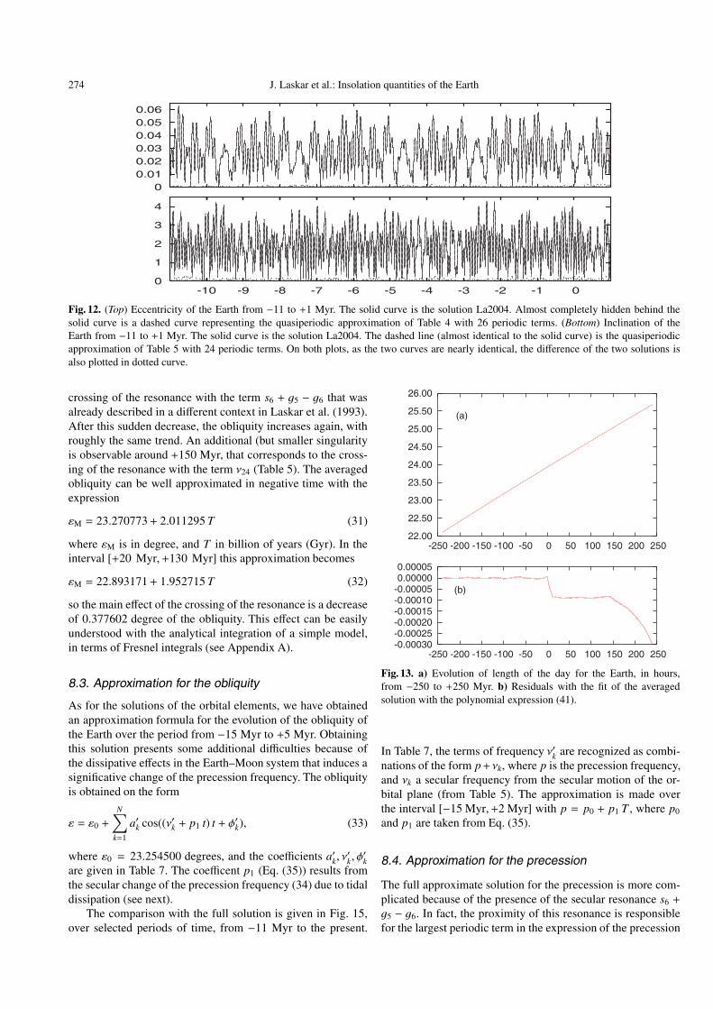
We have plotted in Fig. 14 the evolution of the obliquity ofthe Earth from −250 to +250 Myr. The effect of the tidal dis-sipation is clearly visible on this timescale, and there is a gen-eral increase of the obliquity from −250 Myr to present time.In positive time, there is an obvious singularity in the obliq-uity, with a decrease of about 0.4 degree. This results from the
274 J. Laskar et al.: Insolation quantities of the Earth
Fig. 12. (Top) Eccentricity of the Earth from −11 to +1 Myr. The solid curve is the solution La2004. Almost completely hidden behind thesolid curve is a dashed curve representing the quasiperiodic approximation of Table 4 with 26 periodic terms. (Bottom) Inclination of theEarth from −11 to +1 Myr. The solid curve is the solution La2004. The dashed line (almost identical to the solid curve) is the quasiperiodicapproximation of Table 5 with 24 periodic terms. On both plots, as the two curves are nearly identical, the difference of the two solutions isalso plotted in dotted curve.
crossing of the resonance with the term s6 + g5 − g6 that wasalready described in a different context in Laskar et al. (1993).After this sudden decrease, the obliquity increases again, withroughly the same trend. An additional (but smaller singularityis observable around +150 Myr, that corresponds to the cross-ing of the resonance with the term ν24 (Table 5). The averagedobliquity can be well approximated in negative time with theexpression
εM = 23.270773+ 2.011295 T (31)
where εM is in degree, and T in billion of years (Gyr). In theinterval [+20 Myr,+130 Myr] this approximation becomes
εM = 22.893171+ 1.952715 T (32)
so the main effect of the crossing of the resonance is a decreaseof 0.377602 degree of the obliquity. This effect can be easilyunderstood with the analytical integration of a simple model,in terms of Fresnel integrals (see Appendix A).
8.3. Approximation for the obliquity
As for the solutions of the orbital elements, we have obtainedan approximation formula for the evolution of the obliquity ofthe Earth over the period from −15 Myr to +5 Myr. Obtainingthis solution presents some additional difficulties because ofthe dissipative effects in the Earth–Moon system that induces asignificative change of the precession frequency. The obliquityis obtained on the form
ε = ε0 +
N∑k=1
a′k cos((ν′k + p1 t) t + φ′k), (33)
where ε0 = 23.254500 degrees, and the coefficients a′k, ν′k, φ′k
are given in Table 7. The coefficent p1 (Eq. (35)) results fromthe secular change of the precession frequency (34) due to tidaldissipation (see next).
The comparison with the full solution is given in Fig. 15,over selected periods of time, from −11 Myr to the present.
Fig. 13. a) Evolution of length of the day for the Earth, in hours,from −250 to +250 Myr. b) Residuals with the fit of the averagedsolution with the polynomial expression (41).
In Table 7, the terms of frequency ν′k are recognized as combi-nations of the form p+ νk, where p is the precession frequency,and νk a secular frequency from the secular motion of the or-bital plane (from Table 5). The approximation is made overthe interval [−15 Myr,+2 Myr] with p = p0 + p1 T , where p0
and p1 are taken from Eq. (35).
8.4. Approximation for the precession
The full approximate solution for the precession is more com-plicated because of the presence of the secular resonance s6 +
g5 − g6. In fact, the proximity of this resonance is responsiblefor the largest periodic term in the expression of the precession

J. Laskar et al.: Insolation quantities of the Earth 275
Table 6. Frequency decomposition of the eccentricity of the Earth on the time interval [−15,+5] Myr. For all computations, the data of Table 4should be preferred. Here, e = e0 +
∑20k=1 b′k cos(µ′k t + ϕk) with e0 = 0.0275579. For each term, in the first column is the corresponding
combination of frequencies where gi are the fundamental frequencies (Table 3), and µ j the frequencies of the terms in z from Table 4.
k µ′k (′′/yr) P (yr) b′k ϕ′k (degree)
1 g2 − g5 3.199279 405 091 0.010739 170.739
2 g4 − g5 13.651920 94 932 0.008147 109.891
3 g4 − g2 10.456224 123 945 0.006222 −60.044
4 g3 − g5 13.109803 98 857 0.005287 −86.140
5 g3 − g2 9.909679 130 781 0.004492 100.224
6 µ7 − µ6 0.546076 2 373 298 0.002967 −168.784
7 g1 − g5 1.325696 977 600 0.002818 57.718
8 g4 − g1 12.325286 105 150 0.002050 49.546
9 g2 − g5 + µ6 − µ7 2.665308 486 248 0.001971 148.774
10 g2 − g1 1.883616 688 038 0.001797 137.155
11 µ6 − g5 12.856520 100 805 0.002074 24.487
12 g2 + g4 − 2g5 16.851127 76 909 0.001525 102.380
13 µ6 − g2 9.650041 134 300 0.001491 −167.676
14 2g3 − g4 − g5 12.563233 103 158 0.001316 69.234
15 2g4 − g2 − g3 10.975914 118 077 0.001309 −51.163
16 g1 − g3 11.788709 109 936 0.001300 −146.081
17 µ7 − g2 10.194846 127 123 0.001306 −139.827
18 g3 + g4 − g2 − g5 23.562689 55 002 0.001261 30.098
19 µ7 − g5 13.398519 96 727 0.001344 27.612
20 g2 + g4 − g3 − g5 3.742221 346 318 0.001058 178.662
angle (Fig. 16). The precession angle can thus be approximateby (ψ in arcsec, t in years)
ψ = +49086 + p0 t + p1 t2
+42246ν2
0
(ν0 + 2p1 t)2cos(ν0 t + p1 t2 + φ0) (34)
where
ν0 = 0.150019 ′′/yr
p0 = 50.467718 ′′/yr (35)
p1 = −13.526564−9 ′′/yr2
φ0 = 171.424 degree.
It should be noted that in this formula, the cosine term is anapproximation for a more complicated expression that arisesfrom a double integration of the term cos (ν0 t + p1 t2 + φ0) inthe expression of the derivative of the obliquity (6). In order toobtain an expression as simple as possible, without expressionsinvolving Fresnel integrals (Appendix A), we had to restrain itsinterval of validity to [−15,+2] Myr.
For paleoclimate studies, the usual quantity that relatesmore directly to insolation is the climatic precession e sin ω,where ω = ψ + is the longitude of the perihelion from themoving equinox. We have thus
e sin ω = (z eiψ(t)), (36)
where the decomposition of z = e exp(i ) is provided inTable 4, and the precession angle ψ is given by Eq. (34).
Fig. 14. Evolution of the obliquity of the Earth in degrees, from −250to +250 Myr. The grey zone is the actual obliquity, while the blackcurve is the averaged value of the obliquity over 0.5 Myr time inter-vals. The dotted line is a straight line fitted to the average obliquity inthe past.
The comparison of this approximation with the complete so-lution from −11 to +1 Myr is given in Fig. 17. The solution forclimatic precession is thus on the form
e sin ω =20∑
k=1
bk sin(µkt + ϕk + ψ(t)), (37)
where bk, µk, ϕk are from Table 4, and where ψ(t) is given byEq. (34). The frequencies of the terms of the climatic preces-sion are thus of the form
µ′′k = µk + p + p1 t, (38)
where p, p1 are given in Eqs. (34) and (35).

276 J. Laskar et al.: Insolation quantities of the Earth
Table 7. Approximation for the obliquity of the Earth, following Eq. (33). This expression is not strictly quasiperiodic, because of the presenceof the dissipative term p1 in the evolution of the precesion frequency (33).
k ν′k (′′/yr) P (yr) a′k φ′k (d)
1 p + s3 31.626665 40 978 0.582412 86.645
2 p + s4 32.713667 39 616 0.242559 120.859
3 p + s6 24.124241 53 722 0.163685 −35.947
4 p + ν6 32.170778 40 285 0.164787 104.689
5 p + ν10 31.081475 41 697 0.095382 −112.872
6 p + ν20 31.493347 41 152 0.094379 60.778
7 p + s6 + g5 − g6 0.135393 9 572 151 0.087136 39.928
8 p + s2 43.428193 29 842 0.064348 −15.130
9 p + s1 44.865444 28 886 0.072451 −155.175
10 31.756641 40 810 0.080146 −70.983
11 p + ν13 31.365950 41 319 0.072919 10.533
12 32.839446 39 465 0.033666 −31.614
13 32.576100 39 784 0.033722 77.554
14 32.035200 40 455 0.030677 71.757
15 p + ν8 43.537092 29 768 0.039351 145.835
16 p + ν7 43.307432 29 926 0.030375 160.109
17 p + ν9 43.650496 29 690 0.024733 144.926
18 31.903983 40 622 0.025201 −173.656
19 30.945195 41 880 0.021615 −144.933
20 23.986877 54 030 0.021565 −79.670
21 24.257837 53 426 0.021270 −178.441
22 32.312463 40 108 0.021851 −24.566
23 44.693687 28 997 0.014725 124.744
8.5. Earth–Moon system
In Fig. 18, the evolution of the Earth–Moon semi-major aM axisis plotted over 250 Myr in positive and negative time. The greyarea corresponds to the short period variations of the Earth–Moon distance, obtained in the full integration of the system,while the black curve is the integration of the averaged equa-tions that is used for the precession computations. The agree-ment between the two solutions is very satisfying.
We have searched for a polynomial approximation for thesecular evolution of aM, in order to provide a useful formula forsimple analytical computations. In fact, the Earth–Moon evolu-tion is driven by the tidal dissipation equations (Sect. 4.1), thatinvolve the obliquity of the planet. The important singularity ofthe obliquity in the future (see previous section) prevents fromusing a single approximation over the whole time interval, andwe have used a different polynomial in positive and negativetime.
a−M = 60.142611+6.100887 T−2.709407 T 2
+1.366779 T 3
−1.484062 T 4
a+M = 60.142611+6.120902 T−2.727887 T 2
+1.614481 T 3
−0.926406 T 4
(39)
where T is in billions of years (Gyr), and a+−M in Earth radius(see Table 1). In the residuals plot (Fig. 18b), we can checkthat this polynomial approximation is very precise for negativetime, but in positive time, we have an additional singularityaround 150 Myr, resulting from the secular resonance of theprecession frequency with ν24 (Table 5).
In the same way, it is possible to approximate the evolutionof the precession frequency of the Earth p as the Moon goesaway and the rotation of the Earth slows down with time. Thepolynomial approximation of the precession frequency is thenin arcsec yr−1, with T in Gyr
p− = 50.475838−26.368583 T+21.890862 T 2
p+ = 50.475838−27.000654T+15.603265T 2
. (40)
It should be said that the initial value is kept equal for bothpositive and negative time to avoid discontinuities. It is clearfrom Fig. 19 that for the period between +30 and +130 Myr, abetter approximation could be obtained by adding to the con-stant part the offset +0.135052 arcsec yr−1. It is interesting tonote again the dramatic influence of the resonance ν23 on the

J. Laskar et al.: Insolation quantities of the Earth 277
Fig. 15. Comparison of the solution of the obliquity La2004 (solidline) with its approximation using Table 7 (dotted line) with 26 pe-riodic terms. The difference of two solutions (+22 degrees) is alsoplotted.
evolution of the precession frequency. The equivalent formulasfor the length of the day are (in hours)
LOD− = 23.934468+7.432167 T−0.727046 T 2
+0.409572 T 3
−0.589692 T 4
LOD+ = 23.934468+7.444649 T−0.715049 T 2
+0.458097 T 3. (41)
One should note that Eqs. (39) and (41) correspond at the ori-gin J2000 to a change in the semi major axis of the Moon ofabout 3.89 cm/yr, and a change of the LOD of 2.68 ms/century.These values slightly differ from the current ones of Dickeyet al. (1994) (3.82 ± 0.07 cm/yr for the receding of the Moon).This is understandable, as the Earth–Moon model in our inte-gration that was adjusted to DE406 is simplified with respectto the one of DE406.
9. Stability of the solution
In such long term numerical computations, the sources of er-rors are the error of method due to the limitation of the numer-ical integration algorithm, the numerical roundoff error result-ing from the limitation of the representation of the real numbers
Fig. 16. Comparison of the solution of the precession La2004 with itsapproximation from −15 to +2 Myr. The grey curve is obtained afterremoving uniquely the secular trend ψ0+p0 t+p1 t2. The dark curve arethe residual (in radians) after removing the resonant term (Eq. (34)),which is also displayed in solid line.
Fig. 17. Comparison of the solution of the climatic precessionof La2004 with its approximation from −11 to +1 Myr. The grey curveis the full climatic precession e sin ω. The dark curve are the residualafter removing the approximation given by Eq. (37).
in the computer, and the errors of the initial conditions and ofthe model which are due to our imperfect knowledge of all thephysical parameters in the Solar system, and to the necessarylimitations of the model. Some of the main sources of uncer-tainty in the model for long term integrations were reviewed in(Laskar 1999). The effect of all these errors is amplified by thechaotic behaviour of the system, with an exponential increaseof the difference between two solutions with different settings,until saturation due to the limited range of the considered vari-ables. A summary of these limitations, extracted from (Laskar1999) is given in Table 8, but it should be noted that these timesof validity are probably pessimistic, as they correspond to an-alytical estimates based on the “worst case” situation. Our re-quirement for the precision of a long term solution is also notthe same as for precise short term ephemeris. For the long termsolutions, aimed at paleoclimate or qualitative studies, two so-lutions can be considered as similar, as long as the pattern ofthe two solutions (eccentricity for example), resulting (at firstorder) from the combination of various proper modes remainsimilar. This will last until some of the main proper modes getcompletely out of phase (see Sect. 7). It will be the same forthe solutions in obliquity and precession.

278 J. Laskar et al.: Insolation quantities of the Earth
Fig. 18. a) Evolution of the Earth–Moon semi major axis (in Earthradii) from −250 to +250 Myr. The grey zone is the result of the in-tegration of the full equations, while the black curve is the integrationof the averaged equations, as used in the precession computations;b) residuals with the fit of the averaged solution with the polynomialexpression (39).
Fig. 19. a) Evolution of the precession frequency of the Earth p(in arcsec/yr) −250 to +250 Myr; b) residuals with the fit of the aver-aged solution with the polynomial expression (40).
9.1. Orbital motion
Practically, we have tested the stability of our solution by com-parison of the eccentricity (Fig. 20) and inclination (Fig. 21)with different solutions. In Figs. 20a and 21a, the nominal so-lution La2004 (with stepsize τ = 5 × 10⁻³ years) is comparedto an alternate solution, La2004∗, with the same dynamical
Table 8. Main sources of uncertainty in the orbital solution (fromLaskar 1999). For each limiting factor, an analytical estimate of thetime of validity of the solution TV is given (in Myr), taking into ac-count the exponential growth of the error.
Limiting factor TV
Uncertainty on the masses and intial conditions 38 Myr
Contribution of the main Galilean satellites 35 Myr
Uncertainty in the Earth–Moon system evolution 40 Myr
Effect of the main asteroids 32 Myr
Mass loss of the Sun 50 Myr
Uncertainty of 2 × 10⁻⁷ on the J2 of the Sun 26 Myr
Fig. 20. Stability of the solution for eccentricity of the Earth.a) Difference of the nominal solution La2004 with stepsize τ =5. × 10−3 years, and La2004∗, obtained with τ∗ = 4.8828125 × 10⁻³
years; b) difference of the nominal solution with the solution obtainedwhile setting JS
2 = 0 for the Sun (instead of 2 × 10⁻⁷ in the nominalsolution).
model, and a very close stepsize τ∗ = 4.8828125 × 10⁻³ years(Table 9). This special value was chosen in order that our out-put time span h = 1000 years corresponds to an integer num-ber (204 800) of steps, in order to avoid any interpolation prob-lems in the check of the numerical accuracy. This is thus a testof the time of validity for obtaining a precise numerical solu-tion, resulting from method and roundoff errors of the integra-tor. It is thus limited here to about 60 Myr.
This limitation of 60 Myr is a limitation for the time of va-lidity of an orbital solution, independently of the precision ofthe dynamical model. In order to go beyond this limit, the onlyway will be to increase the numerical accuracy of our compu-tations, by improving the numerical algorithm, or with an ex-tended precision for the number representation in the computer.
A second test is made on the uncertainty of the model.Several sources of uncertainty were listed in (Laskar 1999),and it was found that one of the main sources of uncer-tainty was due to the imprecise knowledge of the Solar
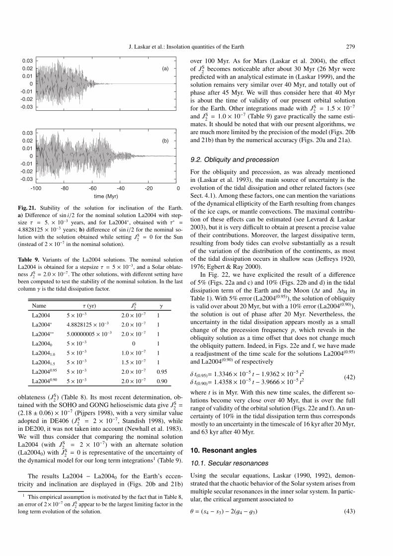
J. Laskar et al.: Insolation quantities of the Earth 279
Fig. 21. Stability of the solution for inclination of the Earth.a) Difference of sin i/2 for the nominal solution La2004 with step-size τ = 5. × 10−3 years, and for La2004∗, obtained with τ∗ =4.8828125 × 10⁻³ years; b) difference of sin i/2 for the nominal so-lution with the solution obtained while setting JS
2 = 0 for the Sun(instead of 2 × 10⁻⁷ in the nominal solution).
Table 9. Variants of the La2004 solutions. The nominal solutionLa2004 is obtained for a stepsize τ = 5 × 10⁻³, and a Solar oblate-ness JS
2 = 2.0 × 10⁻⁷. The other solutions, with different setting havebeen computed to test the stability of the nominal solution. In the lastcolumn γ is the tidal dissipation factor.
Name τ (yr) JS2 γ
La2004 5 × 10⁻³ 2.0 × 10⁻⁷ 1
La2004∗ 4.8828125 × 10−3 2.0 × 10⁻⁷ 1
La2004∗∗ 5.00000005 × 10⁻³ 2.0 × 10⁻⁷ 1
La20040 5 × 10⁻³ 0 1
La20041.0 5 × 10⁻³ 1.0 × 10⁻⁷ 1
La20041.5 5 × 10⁻³ 1.5 × 10⁻⁷ 1
La20040.95 5 × 10⁻³ 2.0 × 10⁻⁷ 0.95
La20040.90 5 × 10⁻³ 2.0 × 10⁻⁷ 0.90
oblateness (JS2 ) (Table 8). Its most recent determination, ob-
tained with the SOHO and GONG helioseismic data give JS2 =
(2.18 ± 0.06) × 10−7 (Pijpers 1998), with a very similar valueadopted in DE406 (JS
2 = 2 × 10⁻⁷, Standish 1998), whilein DE200, it was not taken into account (Newhall et al. 1983).We will thus consider that comparing the nominal solutionLa2004 (with JS
2 = 2 × 10⁻⁷) with an alternate solution(La20040) with JS
2 = 0 is representative of the uncertainty ofthe dynamical model for our long term integrations1 (Table 9).
The results La2004 − La20040 for the Earth’s eccen-tricity and inclination are displayed in (Figs. 20b and 21b)
1 This empirical assumption is motivated by the fact that in Table 8,an error of 2×10⁻⁷ on JS
2 appear to be the largest limiting factor in thelong term evolution of the solution.
over 100 Myr. As for Mars (Laskar et al. 2004), the effectof JS
2 becomes noticeable after about 30 Myr (26 Myr werepredicted with an analytical estimate in (Laskar 1999), and thesolution remains very similar over 40 Myr, and totally out ofphase after 45 Myr. We will thus consider here that 40 Myris about the time of validity of our present orbital solutionfor the Earth. Other integrations made with JS
2 = 1.5 × 10⁻⁷
and JS2 = 1.0 × 10⁻⁷ (Table 9) gave practically the same esti-
mates. It should be noted that with our present algorithms, weare much more limited by the precision of the model (Figs. 20band 21b) than by the numerical accuracy (Figs. 20a and 21a).
9.2. Obliquity and precession
For the obliquity and precession, as was already mentionedin (Laskar et al. 1993), the main source of uncertainty is theevolution of the tidal dissipation and other related factors (seeSect. 4.1). Among these factors, one can mention the variationsof the dynamical ellipticity of the Earth resulting from changesof the ice caps, or mantle convections. The maximal contribu-tion of these effects can be estimated (see Levrard & Laskar2003), but it is very difficult to obtain at present a precise valueof their contributions. Moreover, the largest dissipative term,resulting from body tides can evolve substantially as a resultof the variation of the distribution of the continents, as mostof the tidal dissipation occurs in shallow seas (Jeffreys 1920,1976; Egbert & Ray 2000).
In Fig. 22, we have explicited the result of a differenceof 5% (Figs. 22a and c) and 10% (Figs. 22b and d) in the tidaldissipation term of the Earth and the Moon (∆t and ∆tM inTable 1). With 5% error (La2004(0.95)), the solution of obliquityis valid over about 20 Myr, but with a 10% error (La2004(0.90)),the solution is out of phase after 20 Myr. Nevertheless, theuncertainty in the tidal dissipation appears mostly as a smallchange of the precession frequency p, which reveals in theobliquity solution as a time offset that does not change muchthe obliquity pattern. Indeed, in Figs. 22e and f, we have madea readjustment of the time scale for the solutions La2004(0.95)
and La2004(0.90) of respectively
δ t(0.95)= 1.3346× 10⁻⁵ t − 1.9362 × 10⁻⁵ t2
δ t(0.90)= 1.4358× 10⁻⁵ t − 3.9666 × 10⁻⁵ t2 (42)
where t is in Myr. With this new time scales, the different so-lutions become very close over 40 Myr, that is over the fullrange of validity of the orbital solution (Figs. 22e and f). An un-certainty of 10% in the tidal dissipation term thus correspondsmostly to an uncertainty in the timescale of 16 kyr after 20 Myr,and 63 kyr after 40 Myr.
10. Resonant angles
10.1. Secular resonances
Using the secular equations, Laskar (1990, 1992), demon-strated that the chaotic behavior of the Solar system arises frommultiple secular resonances in the inner solar system. In partic-ular, the critical argument associated to
θ = (s4 − s3) − 2(g4 − g3) (43)

280 J. Laskar et al.: Insolation quantities of the Earth
Fig. 22. Difference in obliquity for different tidal dissipation factor(Table 9): a) La2004 − La2004(0.95); b) La2004 − La2004(0.90). In c)and d), the nominal solution of the obliquity is plotted in solid line,while La2004(0.95) c) and La2004(0.90) d) are in dotted line. After anadjustment of the time scale, the differences of the solutions are muchsmaller over 40 Myr: e) La2004−La2004(0.95) ; f) La2004−La2004(0.90) .
where g3, g4 are related to the precession of the perihelion ofthe Earth and Mars, s3, s4 are related to the precession of thenode of the same planets, is presently in a librational state, butcan evolve in a rotational state, and even move to libration in anew resonance, namely
(s4 − s3) − (g4 − g3) = 0. (44)
This reveals that a region of relatively strong instability resultsfrom the overlap (Chirikov 1979) of these two resonances. Thisresult was questioned by Sussman & Wisdom (1992), as theydid not recover such a large variation for the secular frequen-cies, but reached only 2(s4 − s3) − 3(g4 − g3) = 0 instead ofEq. (44). We have tested these resonant arguments in the nom-inal solution La2004, and in the alternate solutions La2004∗∗,La20040, La20041.5 (Table 9).
In all variants of La2004 (Fig. 23 (top)), the resonant ar-gument corresponding to θ = (s4 − s3) − 2(g4 − g3) was inlibration over the first 40 Myr, while the transition to circu-lation occurred at about 25 Myr in La93. All the solutionsLa2004, La2004∗∗, La20040, La20041.5 differ significantly be-yond 40 to 50 Myr, but they all enter the (s4 − s3) − (g4 −g3) resonance within 100 Myr, comforting the conclusions of
Fig. 23. Resonant arguments (in radians versus time in Myr) θ =(s4 − s3) − 2(g4 − g3) (top) and σ = (g1 − g5) − (s1 − s2) (bottom)for different solutions: a) is the secular solution La93 (Laskar 1990;Laskar et al. 1993) while b) is the present nominal solution La2004.The characteristics of the other variants La20041.5 c), La20040 d),La2004∗∗ e) are listed in Table 9. The arrows indicate the portionsof the solutions when the argument (s4 − s3)− (g4 − g3) is in libration.
(Laskar 1990, 1992). In Fig. 23 (top), the portions of the so-lutions where the argument of (s4 − s3) − (g4 − g3) is in li-bration are pointed by arrows. It should be noted that at leastover 250 Myr, the diffusion seems to remain confined betweenthe resonances (s4 − s3) − 2(g4 − g3) and (s4 − s3) − (g4 − g3).The other important resonant argument ((g1 − g5) − (s1 − s2))that was identified by Laskar (1990, 1992) as the origin of thechaotic behavior of the inner planets presents in all the varia-tions of the numerical solutions La2004, La2004∗∗, La20040,La20041.5 a similar behavior as for the secular solution La93(Fig. 23 (bottom)).
10.2. Geological evidence of chaos
The date of the first transition from libration to circulation ofthe resonant argument related to θ = (s4 − s3) − 2(g4 − g3) isa macroscopic feature displaying the chaotic diffusion of theplanetary orbits. It is thus very tempting to search whether thisfeature could be observed in the geological data that extendnow in continuous records beyond 30 Myr.

J. Laskar et al.: Insolation quantities of the Earth 281
The direct observation of the individual arguments relatedto g3, g4, s3, s4 is certainly out of reach. But it may be possi-ble to follow the evolution in time of the differences g3 − g4
and s3 − s4. Indeed, s3 − s4 appears as a beat of about 1.2 mil-lion of years in the solution of obliquity, as the result of thebeat between the p + s3 and p + s4 components of the obliq-uity, where p is the precession frequency of the axis (see Laskar2004, Fig. 7). In a similar way, g3 − g4 appears as a beat withperiod of about 2.4 Myr in the climatic precession. One under-stands that because of the occurrence of these beats, the detec-tion of the resonant state in the geological data can be possible,as one has to search now for phenomena of large amplitude inthe geological signal. Indeed, in the newly collected data fromOcean Drilling Program Site 926, the modulation of 1.2 Myrof the obliquity appears clearly in the spectral analysis of thepaleoclimate record (Zachos et al. 2001). Moreover, using theODP legs 154 and 199, Pälike et al. (2004) could find someevidence that the critical argument of θ did not show a transi-tion to circulation at 25 Myr, as in La93, but remained in libra-tion over 40 Myr, as in the present new solution La2004. Thisresult is very impressive, although the search for the determina-tion of these resonant angles in the geological data is just start-ing. We may expect that a careful analysis, and new data span-ning the most recent 60 to 100 Myr, will allow to determinethe possible succession of resonant states in the past, allowing,for example, to discriminate between the solutions displayed inFig. 23. Of particular importance would be the detection of thefirst transition from libration to circulation of the resonant ar-gument (s4 − s3) − 2(g4 − g3). This program, if completed, willprovide some extreme constraint for the gravitational model ofthe Solar System. Indeed, the observation of a characteristicfeature of the solution at 40 to 100 Myr in the past, because ofthe exponential divergence of the solutions, will provide a con-straint of 10−4 to 10−10 on the dynamical model of the SolarSystem.
11. Mesozoic timescale
An astronomically calibrated time scale for geological datahas been achieved successfully over the Neogene period(0−23.03 Myr) (Lourens et al. 2004), and the next challengewill be to improve the astronomical precision of the solution, inorder to extend this over the Paleogene (23 to 65 Myr). Beyondthis time length, it is hopeless to expect to obtain a precise so-lution for the orbital elements of the Earth. On the other hand,some features of the solution have a longer time of stability, ifthey are related to the outer planets secular frequencies (Laskar1990).
A very important period present in geological records is the405 kyr period related to the g2 − g5 argument, that is the lead-ing term in the solution of eccentricity (Table 6). In Fig. 24, wehave tested the stability of this argument over the full periodof our integrations, that is over 250 Myr, that extents over theMesozoic geological era (about 65 to 250 Myr). First, we havecompared the argument related to g5 over 3 variants (La2004∗,La20040, La20041.5) of La2004, that reflect both the numeri-cal errors and the errors of the model. This argument, relatedto Jupiter and Saturn is extremely stable, and does not show
Fig. 24. Stability of the g5 (top) and g2 − g5 (bottom) arguments. Thedifference (in radians) of the angles related to g5 and g2 − g5 fromthe nominal solution La2004 and an alternate solution La20041.5 a),La20040 b), and La2004∗ c) (Table 9).
variations of more than 0.05 radians over the full 250 Myrperiod (Fig. 24 (top)). In Fig. 24 (bottom), we have plottedthe same quantities for g2 − g5. The dispersions over 50, 100,and 250 Myr are about 0.3, 1.0, 6.2 radians, that correspond toabsolute error in time respectively of about 20, 70, and 400 kyrover the same periods.
It is thus possible to use this argument, that is visible inmany sedimentary records of the Early Mesozoic (Olsen &Kent 1999, and references therein) as an absolute geologicaltime scale over the whole Mesozoic period. In order to facili-tate the establishment of this timescale, we have searched for abest fit or the period of this argument over all the solutions ofTable 9. Within the uncertainty of this procedure, the best valuefor the frequency g2 − g5 is
ν405 = 3.200′′/yr (45)
which corresponds exactly to a period
P405 = 405 000 yr. (46)
This value differs by less than 0.001′′/yr from the same quan-tity from Table 6, where the direct output of the frequency anal-ysis is given. We propose here that in the establishment of ge-ological timescales, the value 3.200′′/yr should be used. Themaximum error over 50, 100, 200, and 250 Myr should then beless than respectively 30, 150, 350, and 500 kyr. The 405 kyrterm is the largest term of the eccentricity solution. In Fig. 26,the eccentricity of the Earth from La2004, filtered in the
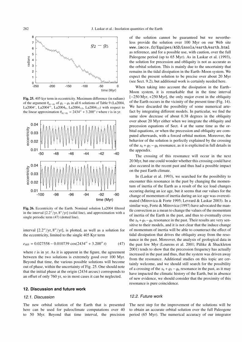
282 J. Laskar et al.: Insolation quantities of the Earth
Fig. 25. 405 kyr term in eccentricity. Maximum difference (in radians)of the argument θg2−g5 of g2 − g5 in all 6 solutions of Table 9 (La2004,La2004∗, La2004∗∗, La20040, La20041.0, La20041.5) with respect tothe linear approximation θg2−g5 = 2434′′ + 3.200′′ t where t is in yr.
Fig. 26. Eccentricity of the Earth. Nominal solution La2004 filteredin the interval [2.2′′/yr, 8′′/yr] (solid line), and approximation with asingle periodic term (47) (dotted line).
interval [2.2′′/yr, 8′′/yr], is plotted, as well as a solution forthe eccentricity, limited to the single 405 Kyr term
e405 = 0.027558− 0.010739 cos(2434′′ + 3.200′′ t) (47)
where t is in yr. As it is apparent in the figure, the agreementbetween the two solutions is extremely good over 100 Myr.Beyond that time, the various possible solutions will becomeout of phase, within the uncertainty of Fig. 25. One should notethat the initial phase at the origin (2434 arcsec) corresponds toan offset of only 760 yr, so in most cases it can be neglected.
12. Discussion and future work
12.1. Discussion
The new orbital solution of the Earth that is presentedhere can be used for paleoclimate computations over 40to 50 Myr. Beyond that time interval, the precision
of the solution cannot be guaranteed but we neverthe-less provide the solution over 100 Myr on our Web sitewww.imcce.fr/Equipes/ASD/insola/earth/earth.htmlas reference, and for a possible use, with caution, over the fullPaleogene period (up to 65 Myr). As in Laskar et al. (1993),the solution for precession and obliquity is not as accurate asthe orbital solution. This is mainly due to the uncertainty thatremains in the tidal dissipation in the Earth–Moon system. Weexpect the present solution to be precise over about 20 Myr(see Sect. 9.2), but additional work is certainly needed here.
When taking into account the dissipation in the Earth–Moon system, it is remarkable that in the time interval[−250 Myr,+250 Myr], the only major event in the obliquityof the Earth occurs in the vicinity of the present time (Fig. 14).We have discarded the possibility of some numerical arte-fact by integrating different models. In particular, we find thesame slow decrease of about 0.38 degrees in the obliquityover about 20 Myr either when we integrate the obliquity andprecession equations of Sect. 4 at the same time as the or-bital equations, or when the precession and obliquity are com-puted afterwards, with a forced orbital motion. Moreover, thebehavior of the solution is perfectly explained by the crossingof the s6 + g5 − g6 resonance, as it is explicited in full details inthe appendix.
The crossing of this resonance will occur in the next20 Myr, but one could wonder whether this crossing could havealso occured in the recent past and thus had a possible impacton the past Earth climate.
In (Laskar et al. 1993), we searched for the possibility toencounter this resonance in the past by changing the momen-tum of inertia of the Earth as a result of the ice load changesoccuring during an ice age, but it seems that our values for thechange of momentum of inertia during an ice age was overesti-mated (Mitrovica & Forte 1995; Levrard & Laskar 2003). In asimilar way, Forte & Mitrovica (1997) have advocated the man-tle convection as a mean to change the values of the momentumof inertia of the Earth in the past, and thus to eventually crossthe s6+g5−g6 resonance in the past. Their results are very sen-sitive to their models, and it is not clear that the induce changeof momentum of inertia will be able to counteract the effect oftidal dissipation that drives the obliquity away from the reso-nance in the past. Moreover, the analysis of geological data inthe past few Myr (Lourens et al. 2001; Pälike & Shackleton2001) tends to show that the precession frequency has actuallyincreased in the past and thus, that the system was driven awayfrom the resonance. Additional studies on this topic are cer-tainly welcome, and we should still search for the possibilityof a crossing of the s6 + g5 − g6 resonance in the past, as it mayhave impacted the climatic history of the Earth, but in absenceof new evidence, we should consider that the proximity of thisresonance is pure coincidence.
12.2. Future work
The next step for the improvement of the solutions will beto obtain an accurate orbital solution over the full Paleogeneperiod (65 Myr). The numerical accuracy of our integrator

J. Laskar et al.: Insolation quantities of the Earth 283
already fulfills this requirement (Fig. 23), although we ex-pect to slightly improve it by switching to extended computerprecision.
The improvement of the model and parameters is muchmore difficult, and will require additional work. First, we willhave to include in our model supplementary contributions in or-der to compare much more closely to DE406. In particular, inthe present work, to save computer time, we had to simplify theinteractions in the Earth–Moon system. In the next integration,we will take into account additional contributions in the bodybody interactions of the Earth–Moon system, and also the li-bration of the Moon. We will also have to adapt the tidal modelin the Earth–Moon system. We will need to take into accountthe effect of the 5 main asteroids that are present in DE406,and probably derive a small model for the contribution of the295 additional asteroids that are considered in DE406. Indeed,the consideration of the main asteroids appears as the nextmost important source of uncertainty for the long term solu-tion (Table 8). Some of the other factors listed in Table 8 caneasily be taken into account, as the consideration of the mainGalilean satellites, or the mass loss of the Sun.
Finally, it will also be important to reestablish the preci-sion of the parameter of the model by a direct comparison tothe observations. For this part, we expect to benefit from theeffort that is developed at present in our laboratory for the im-provement of short time ephemeris devoted to the reduction ofEarth based and space missions observations (Fienga & Simon2004).
The fulfilment of this program will allow to improve onthe main limiting factors listed in Table 8. It should be stressedagain here that the limiting times listed in Table 8 are somewhatpessimistic. We can thus hope that after completing this effort,the orbital solution may be valid over 50 to 65 Myr.
Nevertheless, although this program may lead to a solu-tion valid over about 60 Myr, obtaining a precise solution forthe precession and obliquity of the Earth’s axis over 65 Myris much more difficult, as it will require a modelization of theevolution of the various dissipative contributions (see Sect. 4.1)over this period. An alternate way will be to fit the evolu-tion of the main precession frequency to the geological dataover the Paleogene period. Although some results have beenalready obtained in this direction over some shorter time span(Lourens et al. 2001; Pälike & Shackleton 2001), to extract thevariation of the precession frequency from paleoclimate strati-graphic data is still a challenge, but we hope that the presentpaper will provide a good basis for this future work.
Appendix A: Fresnel integrals and resonances
In this section, we show that Fresnel integrals are very goodapproximations for the crossing of the resonance. Let us de-fine the Fresnel integrals (we have dropped here the usual π/2factor) as
C(x) =∫ x
0cos (t2) dt; S (x) =
∫ x
0sin (t2) dt. (A.1)
Fig. A.1. Fresnel functions C(x) (solid line) and S (x) (dotted line).
We have the expansions, for x ≥ 0 (Abramowitz & Stegun1965)
C(x)=1
2
√π
2− P(x) cos x2 + Q(x) sin x2
S (x)=1
2
√π
2− P(x) cos x2 − Q(x) sin x2
(A.2)
with the asymptotic expansions
P(x) 1
2
1
2x3− 1.3.5
23x7+ · · ·
Q(x) 1
2
1
x− 1
22x5+
1.3.5.7
24x9+ · · ·
.(A.3)
We thus have a jump from the asymptotic value at −∞ to thevalue at +∞ of
√π/2 ≈ 1.253 (Fig. A.1). Due to tidal dis-
sipation, the precession angle evolves in first approximationas Eq. (34)
ψ = ψ0 + p0T + p1T 2 (A.4)
with this evolution, a term of frequency νk + p in Eq. (30) maycross the resonance. In particular, we can compute the contri-bution of the term ν23 in the quasiperiodic decomposition of ζ(Table 5). We will have from Eq. (28),
dε
dt
∣∣∣∣∣∣∣23
= −2a23ν23 sin((ν23 + p0)t + p1t2 + φ23 + ψ0). (A.5)
More generally, for a > 0, the integral of
sin (a t2 + b t + c) (A.6)
is
1√a
cos(δ)S
x +
b
2a
√a
+ sin(δ)C
x +
b
2a
√a
, (A.7)
where δ = c − b2/4a, and the asymptotic offset ∆(ε) due to thecrossing of the resonance of the term (A.6) is easily obtained as
∆(ε) =
√π
acos
δ − π4
· (A.8)
With the data for the resonant term ν23, we have
a = p1; b = ν23 + p0; c = φ23 + ψ0, (A.9)

284 J. Laskar et al.: Insolation quantities of the Earth
Fig. A.2. Obliquity variation (in degree) versus time resulting from thecrossing of the resonance in the ν23 term (solid line). In the same plot,the dependence of the precession phase is illustrated. for δ = −π/4 theobliquity offset is null (dashed line) while it is maximal for δ = +π/4.The nominal solution (solid line) corresponds nearly to a maximaldecrease of the obliquity.
and as the term is of amplitude −2a23ν23, we obtain (Fig. A.2)an offset of amplitude
∆(ε)23 ≈ −0.398046 deg (A.10)
that is very close to the value 0.377602 deg obtained in Sect. 8.3for the complete integration. It should be noted that the ampli-tude of the offset depends critically of the phase c = φ23 + ψ0.Indeed, a maximum amplitude for the offset will be obtainedwhen δ = π/4 mod(π) , which leads to∣∣∣∆(ε)
23
∣∣∣max= 2a23ν23
√π/p1 ≈ 0.398721 deg. (A.11)
while no offset will occur when δ = −π/4 mod(π). In thepresent case, the actual value of the offset is thus close toits maximum possible value. One should also note that apartfrom the drift that occurs at the resonance, which ranges fromabout −0.4 to +0.4 degree, the maximum oscillation of theobliquity is of about 0.1 degree (Fig. A.2).
Acknowledgements. J.L. thanks J. Landwehr for providing a copyof Pilgrim’s work, A. Vernekar for a copy of his monograph, andH. Pälike for his comments. This work benefited from support fromINSU-CNRS, PNP-CNRS, and CS, Paris Observatory.
References
Adhémar, J. 1842, Révolutions de la mer, (Paris: Bachelier)Agassiz, L. 1840, Études sur les glaciers (Paris)Arnold, V. I., Kozlov, V. V., & Neishtadt, A. I. 1988, Mathematical
aspects of classical and celestial mechanics, Dyn. Systems III, ed.V. I. Arnold (New York: Springer)
Berger, A. L. 1978, J. Atmos. Sci., 35, 2362Bills, B. G. 1994, Geophys. Res. Lett., 21(3), 177Bretagnon, P. 1974, A&A, 30, 141Bretagnon, P. 1984, Celest. Mech., 34, 193Bretagnon, P., & Simon, J.-L. 1990, A&A, 239, 387Brouwer, D., & Van Woerkom, A. J. J. 1950, Astron. Papers Am.
Ephem., XIII, Part II, 81Chapman, S., & Lindzen, R. S. 1970, Atmospheric tides (Dordrecht:
D. Reidel)
Chirikov, B. 1979, Phys. Rep., 52, 263Correia, A., & Laskar, J. 2003, J. Geophys. Res., 108(E11), 5123Correia, A., Laskar, J., & Néron de Surgy, O. 2003, Icarus, 163, 1Croll, J. 1890, Climate and Time (London)Darwin, G. H. 1880, Philos. Trans. R. Soc. London, 171, 713Dickey, J. O., Bender, P. L., Faller, et al. 1994, Science, 265, 182Duriez, L. 1977, A&A, 54, 93Egbert, G. D., & Ray, R. D. 2000, Nature, 405, 775Fienga, A., & Simon, J.-L. 2004, submittedForte, A., & Mitrovica, J. X. 1997, Nature, 390, 676Gradstein, F., Ogg, J., & Smith, A. 2004, A Geologic Time Scale 2004
(UK: Cambridge University Press), in pressHaretu, S. C. 1885, Annales de l’Observatoire de Paris, 18, I1Harzer, P. 1895, Die Säcularen veränderungen der bahnen der grossen
planeten, Fürstlich Jablonowski’schen Gesellschaft, LeipzigHays, J. D., Imbrie, J., & Schackleton, N. J. 1976, Science, 194, 1121Hill, G. 1897, AJ, 17(11), 81Imbrie, J. 1982, Icarus, 50, 408Imbrie, J., & Imbrie, K. P. 1979, Ice Ages: Solving the Mystery (MA:
Harvard University Press)Ito, T., & Tanikawa, K. 2002, MNRAS, 336, 483Ito, T., Masuda, K., Hamano, Y., & Matsui, T. 1995, J. Geophys. Res.,
100, 15147Jeffreys, H. 1920, Phil. Trans. R. Soc. London, Ser. A, 221, 239Jeffreys, H. 1976, The Earth, Its Origin, History, and Physical
Constitution, 6th ed. (Cambridge, UK: Cambridge UniversityPress)
Kinoshita, H. 1977, Cel. Mech., 15, 277Lagrange, J. L. 1774, Oeuvres complètes, t. IV, Gauthier-Villars, Paris,
1869, 111Lagrange, J. L. 1776, Oeuvres complètes, t. IV, Gauthier-Villars, Paris,
1869, 255Lagrange, J. L. 1777, Oeuvres complètes, t. VI, Gauthier-Villars,
Paris, 1873, 633Lagrange, J. L. 1781, Oeuvres complètes, t. V, Gauthier-Villars, Paris,
1870, 125Lagrange, J. L. 1782, Oeuvres complètes, t. V, Gauthier-Villars, Paris,
1870, 211Lambeck, K. 1980, The Earth’s variable rotation (UK: Cambridge
University Press)Lambeck, K. 1980, Geophysical Geodesy (UK: Oxford University
Press)Laplace, P. S. 1773–1776, Oeuvres complètes, t. VIII, Gauthier-
Villars, Paris, 1891, 199Laplace, P. S. 1776, Oeuvres complètes, t. VIII, Gauthier-Villars,
Paris, 1891, 369Laskar, J. 1984, Théorie générale planétaire: Eléments orbitaux des
planètes sur 1 million d’années, Thèse, Observatoire de ParisLaskar, J. 1985, A&A, 144, 133Laskar, J. 1986, A&A, 157, 59Laskar, J. 1988, A&A, 198, 341Laskar, J. 1989, Nature, 338, 237Laskar, J. 1990, Icarus, 88, 266Laskar, J. 1992, in Chaos, resonance and collective dynamical phe-
nomena in the solar system, Ferraz-Mello, S. (1) (Kluwer Acad.Publ.), IAU Symp., 152
Laskar, J. 1999, Phil. Trans. R. Soc. Lond. A., 357, 1735Laskar, J. 1999, Introduction to frequency map analysis, in NATO
ASI 533 3DHAM95, S’Agaro, Spain, C. Simò (Kluwer), 134Laskar, J. : 2001, Astronomical Solutions for Paleoclimate Studies,.
AGU Fall Meeting 2001 Abstracts U11A-01Laskar, J. 2003, Ann. Henri Poincaré, 4, Suppl. 2, S693Laskar, J. 2003, in Hamiltonian systems and Fourier analysis, ed.
Benest et al. (Taylor, Francis), in press

J. Laskar et al.: Insolation quantities of the Earth 285
Laskar, J., Joutel, F., & Boudin, F. 1993, A&A, 270, 522Laskar, J., & Robutel, P. 2001, Celest. Mech., 80, 39Laskar, J., Correia, A. C. M., Gastineau, M., et al. 2004, Icarus, 170,
343Le Verrier, U. 1856, Ann. Obs. Paris, II, Mallet-Bachelet, ParisLevrard, B., & Laskar, J. 2003, Journal Geophys. Int., 154, 970Lourens, L. J., Wehausen, R., & Brumsack, H. J. 2001, Nature, 409,
1029Lourens, L. J., Hilgen, F. J., Shackleton, N. J., Laskar, J., & Wilson,
D. 2004, in The Neogene Period, ed. F. Gradstein, J. Ogg, & A.Smith, A Geologic Time Scale 2004 (UK: Cambridge UniversityPress), in press
Lumb, L. I., & Aldridge, K. D. 1991, J. Geomagn. Geoelectr., 43, 93MacCarthy, D. D. 1992, IERS Standards, IERS Technical note 13,
Observatoire de ParisMacCarthy, D. D., & Petit, G. 2004, IERS Standards, IERS Technical
note 13, Observatoire de ParisMignard, F. 1979, The Moon and the Planets, 20, 301Mignard, F. 1980, The Moon and the Planets, 23, 185Mignard, F. 1981, The Moon and the Planets, 24, 189Milani, A., Nobili, A. N., & Carpino, M. 1987, A&A, 172, 265Milankovitch, M. 1941, Kanon der Erdbestrahlung und seine
Andwendung auf das Eiszeitenproblem, Royal Serbian AcademyMitrovica, J. X., & Forte, A. 1995, Geophys. J. Int., 121, 21Néron de Surgy, O., & Laskar, J. 1997, A&A, 318, 975Newhall, X. X., Standish, E. M., & Williams, J. G. 1983, A&A, 125,
150Olsen, P., & Kent, D. 1999, Phil. Trans. R. Soc. London, Ser. A., 357,
1761Pälike, H. 2002, Thesis, University of CambridgePälike, H., & Shackleton, N. J. 2001, EPSL, 400, 1029Pälike, H., Laskar, J., & Shackleton, N. J. 2004, Geological constraints
on the chaotic diffusion of the Solar System, Geology, in pressPijpers, F. P. 1998, MNRAS, 297, L76Pilgrim, L. 1904, Versuch einer rechnerischen behandlung des
eiszeitenproblems. Jahreshefte fur vaterlandische Naturkunde inWurttemberg, 60
Poincaré, H. 1893, Méthodes nouvelles de la mécanique céleste,(Paris: Gauthier-Villars), Vol. II
Poincaré, H. 1910, Bull. Astron., 27, 321Pontécoulant, G. de 1834, Théorie Analytique du Système du Monde,
t. III, Bachelier, ParisQuinn, T. R., Tremaine, S., & Duncan, M. 1991, AJ, 101, 2287Rochester, M. G. 1976, Geophys. J. R. A. S., 46, 109Rubincam, D. P. 1990, Science, 248, 720Rubincam, D. P. 1995, Paleoceanography, 10, 365Saha, P., & Tremaine, S. 1994, AJ, 108 (5), 1962Sharav, S. G., & Boudnikova, N. A. 1967a, Bull. I.T.A, XI-4(127), 231Sharav, S. G., & Boudnikova, N. A. 1967b, Trud. I.T.A, XIV, 48Standish, E. M. 1998, JPL planetary and Lunar ephemerides,
DE405/LE405. JPL IOM 312.F-98-048, PasadenaStockwell, J. N. 1873, Memoir on the secular variations of the ele-
ments of the eight principal planets. Smith. Contr. Knowledge,Washington, 18
Sussman, G. J., & Wisdom, J. 1992, Science, 257, 56Touma, J., & Wisdom, J. 1994, AJ, 108, 1943Varadi, F., Bunnegar, B., & Ghil, M. 2003, ApJ, 592, 620Vernekar 1972, Long-period global variations of incoming solar radi-
ation, Meteorol. Monogr., 12Volland, H. 1978, Earth’s rotation from eons to days, ed. Brosche and
Sündermann (Springer), 62Williams, D. M., Kasting, J. F., & Frakes, L. A. 1998, Nature, 396,
453Williams, J. G., Boggs, D. H., Yoder, C. F., Ratcliff, J. T., & Dickey,
J. O. 2001, J. Geophys. Res., 106, 27933Wisdom, J., & Holman, M. 1991, AJ, 102(4), 128Yoder, C. F. 1995, Astrometric and geodetic properties of Earth and
the Solar System, in ed. T. J. Ahrens, Global Earth Physics: AHandbook of Physical Constants, American Geophysical Union,Washington DC, 1
Zachos, J. C., Shackleton, N. J., Revenaugh, J. S., Pälike, H., &Flower, B. P. 2001, Science, 292, 274
Zachos, J. C., Pagani, M., Sloan, L., Thomas, E., & Billups, K. 2001,Science, 292, 686